Frustration-free free fermions

Abstract

We develop a general theory of frustration-free free-fermion systems and derive their necessary and sufficient conditions. Assuming locality and translation invariance, we find that the possible band touching between the valence bands and the conduction bands is always quadratic or softer, which rules out the possibility of describing Dirac and Weyl semimetals using frustration-free local Hamiltonians. We further construct a frustration-free free-fermion model on the honeycomb lattice and show that its density fluctuations acquire an anomalous gap originating from the diverging quantum metric associated with the quadratic band-touching points. Nevertheless, an $O(1/L^{2})$ finite-size scaling of the charge-neutral excitation gap can be verified even in the presence of interactions, consistent with the more general results we derive in an accompany work [arXiv:2503.12879].

Introduction—Frustration is a common enabler for exotic quantum phases of matter. In lattices like the kagome and pyrochlore, geometric frustration in the nearest-neighbor models results in destructive interference which quenches the kinetic energy of the electrons and leads to completely flat bands. In spin liquids, energetic frustration disfavors conventional magnetic orders and leads to highly entangled quantum disordered ground states hosting fractionalized excitations like anyons.

More technically, we say a Hamiltonian is frustration-free if all the local terms are simultaneously minimized by the ground states [1]. Frustration-freeness serves as a powerful starting point for deriving general results about both the ground state and the excitation spectrum of the system—a rare possibility for quantum many-body problems. Restrictive as it may seem, a surprisingly diverse array of quantum phases could be realized using frustration-free Hamiltonains. Many important spin models, such as the Affleck–Kennedy–Lieb–Tasaki model [2, 1], the Majumdar–Ghosh (MG) model [3, 4], and more generally the parent Hamiltonians of matrix product states [5, 6] are all frustration-free.

Paradoxical as it may seem, frustration-free models also serve as important theoretical tools for investigating exotic quantum phases associated with geometric frustration. Examples include the Rokhsar-Kivelson model [7] for quantum critical points and the Kitaev toric code models [8] for quantum spin liquids, as well as the free-fermion nearest-neighbor hopping models on the kagome, pychlore, and other line-graph lattices [9, 10, 11, 12, 13, 14, 15, 16, 17, 18, 19, 20]. The frustration-freeness also allows one to derive rigorous results about the nature of the ground state(s) when electron-electron interaction is incorporated [9, 10, 12, 14, 11, 13, 21, 22, 23], as exemplified by the saturated ferromagnetism in partially filled flat bands [1]. These results are particularly relevant in recent years due to the emergence of tunable flat-band materials in both natural [24, 25, 26, 27, 28, 29, 30, 31, 32, 33, 34, 35, 36] and artificial [37, 38, 39, 40, 41, 42] platforms. Existing general results on frustration-free Hamiltonians typically concern bosonic systems like quantum magnets [43, 44, 45, 46, 47, 48, 49, 50]. Motivated by the recently highlighted connections between frustration-freeness, flat bands, and correlated topological materials [1, 51, 52], we develop a general theory for frustration-free free fermions (F⁴) in this work.

Frustration-free conditions—We begin by deriving the F⁴ conditions for particle-number conserving Hamiltonians. Consider a free-fermion Hamiltonian $\hat{H}$ defined on a lattice

$$\hat{H}=\sum_{\bm{R}}\hat{H}_{\bm{R}};\quad\hat{H}_{\bm{R}}=\hat{\bm{c}}_{\bm{R}}^{\dagger}h_{\bm{R}}\hat{\bm{c}}_{\bm{R}}+C_{\bm{R}}.$$ (1)

Here, $\hat{H}_{\bm{R}}$ is a local term defined around the point $\bm{R}$, $\hat{\bm{c}}_{\bm{R}}$ is an $N_{r}$-dimensional column vector with components being the $\hat{c}_{\bm{r}\sigma}$ within a range $|\bm{r}-\bm{R}|<r$, and $\sigma$ labels the fermion modes (say sublattices, orbitals, and spin) assigned to $\bm{r}$. We assume $\hat{H}$ is local in the sense that $r$ is finite and independent of the system size. The fermion hopping amplitudes are encoded in the $N_{r}$-dimensional Hermitian matrices $h_{\bm{R}}$. The constant $C_{\bm{R}}$ will be fixed later.

Let $\mu_{\bm{R}\alpha}>0$ ($\alpha=1,2,\cdots,A_{\bm{R}}$) be positive eigenvalues of $h_{\bm{R}}$ and $\bm{\psi}_{\bm{R}\alpha}$ be the corresponding normalized eigenvectors. Likewise, let $-\nu_{\bm{R}\beta}<0$ ($\beta=1,2,\cdots,B_{\bm{R}}$) and $\bm{\phi}_{\bm{R}\beta}$ be the negative eigenvalues and associated eigenvectors. $h_{\bm{R}}$ might admit null vectors but they will not be used. We define corresponding annihilation operators by

$$\hat{\psi}_{\bm{R}\alpha}\coloneqq\bm{\psi}_{\bm{R}\alpha}^{\dagger}\hat{\bm{c}}_{\bm{R}},\quad\hat{\phi}_{\bm{R}\beta}\coloneqq\bm{\phi}_{\bm{R}\beta}^{\dagger}\hat{\bm{c}}_{\bm{R}}.$$ (2)

Fermions with the same label $\bm{R}$ satisfy canonical anticommutation relations due to the orthonormality of the eigenvectors. Also, as both $\hat{\psi}$ and $\hat{\phi}$ are sums of fermion annihilation operators, for any $\bm{R},\bm{R}^{\prime}$ we have

$$\{\hat{\psi}_{\bm{R}\alpha},\hat{\psi}_{\bm{R}^{\prime}\alpha^{\prime}}\}=\{\hat{\phi}_{\bm{R}\beta},\hat{\phi}_{\bm{R}^{\prime}\beta^{\prime}}\}=\{\hat{\psi}_{\bm{R}\alpha},\hat{\phi}_{\bm{R}^{\prime}\beta}\}=0.$$ (3)

For $\bm{R}\neq\bm{R}^{\prime}$, however, $\{\hat{\psi}_{\bm{R}\alpha},\hat{\psi}_{\bm{R}^{\prime}\alpha^{\prime}}^{\dagger}\}$, $\{\hat{\phi}_{\bm{R}\beta},\hat{\phi}_{\bm{R}^{\prime}\beta^{\prime}}^{\dagger}\}$, and $\{\hat{\psi}_{\bm{R}\alpha},\hat{\phi}_{\bm{R}^{\prime}\beta}^{\dagger}\}$ for $\bm{R}\neq\bm{R}^{\prime}$ do not vanish generally.

Setting $C_{\bm{R}}=\sum_{\beta}\nu_{\bm{R}\beta}$, the local Hamiltonian can be rewritten as $\hat{H}_{\bm{R}}=\hat{H}_{\bm{R}}^{(+)}+\hat{H}_{\bm{R}}^{(-)}$ with

$$\hat{H}_{\bm{R}}^{(+)}\coloneqq\sum_{\alpha=1}^{A_{\bm{R}}}\mu_{\bm{R}\alpha}\hat{\psi}_{\bm{R}\alpha}^{\dagger}\hat{\psi}_{\bm{R}\alpha},\quad\hat{H}_{\bm{R}}^{(-)}\coloneqq\sum_{\beta=1}^{B_{\bm{R}}}\nu_{\bm{R}\beta}\hat{\phi}_{\bm{R}\beta}\hat{\phi}_{\bm{R}\beta}^{\dagger}.$$ (4)

Note that both $\hat{\psi}_{\bm{R}\alpha}^{\dagger}\hat{\psi}_{\bm{R}\alpha}$ and $\hat{\phi}_{\bm{R}\beta}\hat{\phi}_{\bm{R}\beta}^{\dagger}=1-\hat{\phi}_{\bm{R}\beta}^{\dagger}\hat{\phi}_{\bm{R}\beta}$ are projectors with eigenvalues $0$ and $1$. Therefore, $\hat{H}_{\bm{R}}$ is positive semi-definite. As the choice of the constants $C_{\bm{R}}$ is immaterial, our discussion up to this point applies generally to any number-conserving free-fermion problems.

We now introduce our first F⁴ result. Recall a local Hamiltonian $\hat{H}$ is frustration-free if there exists a split $\hat{H}=\sum_{\bm{R}}\hat{H}_{\bm{R}}$ with positive-semidefinite local terms $\hat{H}_{\bm{R}}$ and a state $|\Phi\rangle$ such that $\hat{H}_{\bm{R}}|\Phi\rangle=0$ for all $\bm{R}$ simultaneously [1]. We claim a free-fermion $\hat{H}$ expressed as in Eq. (4) is frustration-free if and only if

$$\{\hat{\psi}_{\bm{R}\alpha},\hat{\phi}_{\bm{R}^{\prime}\beta}^{\dagger}\}=0\quad\text{for all $\bm{R}$, $\bm{R}^{\prime}$, $\alpha$, $\beta$.}$$ (5)

To appreciate the validity of the condition, we note that if $\hat{H}$ is F⁴ then its ground state $|\Phi\rangle$ satisfies $\hat{\psi}_{\bm{R}\alpha}|\Phi\rangle=\hat{\phi}_{\bm{R}^{\prime}\beta}^{\dagger}|\Phi\rangle=0$ for all $\bm{R},\alpha,\beta$. As $\{\hat{\psi}_{\bm{R}\alpha},\hat{\phi}_{\bm{R}^{\prime}\beta}^{\dagger}\}$ is a $\mathbb{C}$-number, the existence of $|\Phi\rangle$ implies the anti-commutator vanishes. In the other direction, one can first define a state $|\Phi\rangle$ by applying all of the linearly independent fermion creation operators among the set $\{\hat{\phi}_{\bm{R},\beta}^{\dagger}\}_{\bm{R},\beta}$ to the vacuum [53]. The vanishing of the anti-commutator in Eq. (5) implies $|\Phi\rangle$ is annihilated by all $\hat{H}_{\rm R}$, proving $\hat{H}$ is F⁴.

We note that the condition Eq. (5) also extends naturally to fermionic bilinear Hamiltonians without particle U(1) symmetry, as we discuss in Ref. [53].

Dirac trick—It is generally known that Dirac-like Hamiltonians on a bipartite lattice are related to frustration-free models defined on its sublattices. For instance, the F⁴ model on the checkerboard lattice can be obtained by squaring the single-particle Hamiltonian associated with the Lieb lattice [54, 9, 10]. We now show that similar relations can be obtained for any F⁴ models.

From the split in Eq. (4), we can write the full Hamiltonian as $\hat{H}=\hat{H}^{(+)}+\hat{H}^{(-)}$, where $\hat{H}^{(\pm)}=\sum_{\bm{R}}\hat{H}^{(\pm)}_{\bm{R}}$. By construction, the non-zero single-particle energies $\omega^{(+)}_{\gamma}$ associated with $\hat{H}^{(+)}$ (resp. $\omega^{(-)}_{\gamma}$ for $\hat{H}^{(-)}$) are all positive (negative). Furthermore, if $\hat{H}$ is F⁴, Eq. (5) implies $[\hat{H}_{\bm{R}}^{(+)},\hat{H}_{\bm{R}^{\prime}}^{(-)}]=0$ and therefore the non-zero single-particle energies of $\hat{H}$ can be obtained by combining those from $\hat{H}^{(\pm)}$.

We now show that the non-zero single-particle energies can always be written as $\omega^{(\pm)}_{\gamma}=\pm\left(\nu^{(\pm)}_{\gamma}\right)^{2}$, where $\nu^{(\pm)}$ are obtained from the associated Dirac-like Hamiltonian. For concreteness, we focus on $\hat{H}^{(+)}$ below and the construction for $\hat{H}^{(-)}$ is similar. From the form in Eq. (4), we can construct an auxiliary Hamiltonian $\hat{\tilde{H}}^{(+)}=\sum_{\bm{R}}\hat{\tilde{H}}_{\bm{R}}^{(+)}$, where

$$\begin{split}\hat{\tilde{H}}_{\bm{R}}^{(+)}=\left(\begin{array}[]{cc}\hat{\bm{c}}_{\bm{R}}^{\dagger}&\hat{\bm{d}}_{\bm{R}}^{\dagger}\end{array}\right)\left(\begin{array}[]{cc}0&\bm{\psi}_{\bm{R}}\sqrt{\mu_{\bm{R}}}\\ \sqrt{\mu_{\bm{R}}}\bm{\psi}_{\bm{R}}^{\dagger}&0\end{array}\right)\left(\begin{array}[]{c}\hat{\bm{c}}_{\bm{R}}\\ \hat{\bm{d}}_{\bm{R}}\end{array}\right).\end{split}$$ (6)

Here, $\hat{\bm{d}}_{\bm{R}}=(\hat{d}_{\bm{R}1},\hat{d}_{\bm{R}2},\dots,\hat{d}_{\bm{R}A_{\bm{R}}})^{T}$ is a vector of auxiliary fermion annihilation operators introduced at $\bm{R}$, $\mu_{\bm{R}}$ is a diagonal matrix consisting of the original local eigenvalues $\mu_{\bm{R}\alpha}>0$ for $\alpha=1,\dots,A_{\bm{R}}$, and $\psi_{\bm{R}}$ is an $N_{r}\times A_{\bm{R}}$ dimensional matrix formed by the eigenvectors $\bm{\psi}_{\bm{R}\alpha}$ of $h_{\bm{R}}$. As defined, $\hat{\tilde{H}}^{(+)}$ is a local Hamiltonian with chiral symmetry, and so its non-zero single-particle energies come in pairs of the form $\pm\nu^{(+)}_{\gamma}$. Although the “square root” is taken for each local term $\hat{H}_{\bm{R}}^{(+)}$, one can verify that the decoupled block in $\left(\tilde{h}^{(+)}\right)^{2}$ acting on the $\hat{c}$-fermions is identical to the single-particle Hamiltonian $h^{(+)}$ of the original problem (Appendix A). This establishes $\omega^{(+)}=\left(\nu^{(+)}_{\gamma}\right)^{2}$.

Excitation gap—Our next result concerns the finite-size scaling of the excitation gap of F⁴ Hamiltonians. Consider a family of F⁴ Hamiltonians $\{\hat{H}(L)\}$ labeled by the finite linear size $L$. Let $\epsilon(L)>0$ be the first non-zero eigenvalue of $\hat{H}(L)$. We say the system is gapless if $\epsilon(L)$ approaches $0$, the ground-state energy, in the thermodynamic limit. In the following, we use the Dirac trick to prove that $\epsilon(L)\sim O(1/L^{2})$ for gapless F⁴ Hamiltonians with particle U(1) and lattice translation symmetries.

From the F⁴ condition, $[\hat{H}^{(+)},\hat{H}^{(-)}]=0$ and so the Bloch Hamiltonians associated with $\hat{H}^{(+)}$ and $\hat{H}^{(-)}$ commute at every momentum $\bm{k}$ in the Brillouin zone (BZ). The mentioned non-zero single-particle energies of $\hat{H}$ can then be labeled by the momentum $\bm{k}$ as $\omega^{(\pm)}_{\bm{k},n}$, where $n=1,2,\dots$ is counted from zero energy. Furthermore, the auxiliary Dirac-like Hamiltonians are also translation-invariant, and we have the momentum-resolved relation $\omega^{(\pm)}_{\bm{k},n}=\pm\left(\nu_{\bm{k},n}^{(\pm)}\right)^{2}$. This reveals the non-zero bands of any F⁴ model can always be understood as the square of some auxiliary bands.

If $\hat{H}$ is gapless, at least one of $\nu_{\bm{k},1}^{(+)}$ and $\nu_{\bm{k},1}^{(-)}$ must vanish at some momentum $\bm{k}_{*}$. Consider a small line segment $\bm{k}=\bm{k}_{*}+\delta k\hat{\bm{\kappa}}$ passing through $\bm{k}_{*}$ for any direction $\hat{\bm{\kappa}}$. As the auxiliary Hamiltonians only contain finite-range hopping, with suitable labeling the dispersion $\nu^{(\pm)}_{\bm{k},n}$ can also be expanded analytically in $\delta k$ [55]. Now, if $\nu_{\bm{k}_{*},1}^{(+)}=0$, we have $\nu^{(+)}_{\bm{k},1}=v_{\hat{\bm{\kappa}}}\delta k+O(\delta k^{2})$ for some velocity component $v_{\hat{\bm{\kappa}}}$. We can then conclude a quadratic dispersion $\omega_{\bm{k}1}^{(+)}=v_{\hat{\bm{\kappa}}}^{2}\delta k^{2}+\mathcal{O}(\delta k^{3})$ around $\bm{k}=\bm{k}_{0}+\delta k\hat{\bm{\kappa}}$. The $O(1/L^{2})$ finite-size scaling of excitation energy then follows from the discrete sampling of the BZ.

We also comment briefly on the case without translation symmetry. A main difficulty in this case is the lack of a simple way to define a sequence of Hamiltonians $\{\hat{H}(L)\}$ approaching the thermodynamic limit. Yet, if we assume the weaker condition $\epsilon(L)\sim O(1/L)$ for local free-fermion Hamiltonians, then the stronger conclusion $\epsilon(L)\sim O(1/L^{2})$ for F⁴ Hamiltonians follows from the Dirac trick.

Honeycomb model—We now illustrate our results through an example. Consider spinless fermions hopping on the two-dimensional honeycomb lattice with one $s$ orbital per site (Fig. 1). As is realized in graphene, there are symmetry-protected band touchings at the K and K’ points. Although linear dispersion is generally expected, our results imply any F⁴ Hamiltonians on the honeycomb must have the Dirac fermions softened into band touching points that are quadratic or softer. In other words, the F⁴ requirement automatically tunes the Dirac velocity to zero, as we show below in a concrete model.

Let $\hat{c}^{\dagger}_{{\bm{R}},\sigma}$ for $\sigma=A,B$ be spinless fermions defined on the $\sigma$ site of unit cell ${\bm{R}}$. We consider a finite $L$-by-$L$ lattice along the two lattice vectors. Based on the F⁴ condition Eq. (5), we define compactly supported fermions $\hat{\psi}_{\bm{R}}$ and $\hat{\phi}_{\bm{R}}$ by taking superposition of the six orbitals around a hexagon, as shown in Fig. 1 (a,b). One can verify $\{\hat{\psi}_{\bm{R}},\hat{\phi}_{\bm{R}^{\prime}}^{\dagger}\}=0$ and therefore the Hamiltonain $\hat{H}=t\sum_{\bm{R}}\left(\hat{\psi}_{\bm{R}}^{\dagger}\hat{\psi}_{\bm{R}}+\hat{\phi}_{\bm{R}}\hat{\phi}_{\bm{R}}^{\dagger}\right)$ is F⁴.

Upon Fourier transform with $\hat{c}_{{\bm{k}},\sigma}^{\dagger}=\frac{1}{L}\sum_{{\bm{R}}}\hat{c}_{{\bm{R}},\sigma}^{\dagger}e^{i{\bm{k}}\cdot{\bm{R}}}$, one finds

$$\begin{split}\hat{\psi}_{{\bm{k}}}^{\dagger}=\hat{\bm{c}}^{\dagger}_{{\bm{k}}}{\bm{\psi}}_{{\bm{k}}};\quad{\bm{\psi}}_{{\bm{k}}}=\frac{1}{\sqrt{6}}\left(\begin{array}[]{c}1+e^{i2\pi k_{2}}+e^{i2\pi(k_{1}+k_{2})}\\ 1+e^{i2\pi k_{1}}+e^{i2\pi(k_{1}+k_{2})}\end{array}\right),\end{split}$$ (7)

where we write ${\bm{k}}=k_{1}{\bm{b}}_{1}+k_{2}{\bm{b}}_{2}$ with ${\bm{b}}_{1,2}$ denoting the reciprocal lattice vectors and $\hat{\bm{c}}^{\dagger}_{{\bm{k}}}=(\hat{c}_{{\bm{k}},A}^{\dagger},\hat{c}_{{\bm{k}},b}^{\dagger})$. $\hat{\phi}_{{\bm{k}}}^{\dagger}$ is similarly defined but with ${\bm{\phi}}_{{\bm{k}}}=\sigma_{3}{\bm{\psi}}_{{\bm{k}}}$. Here, $\sigma_{3}$ is the Pauli matrix in the sublattice space. Since the fermions defined for different unit cells do not generally anti-commute with each other, ${\bm{\psi}}_{{\bm{k}}}$ and ${\bm{\phi}}_{{\bm{k}}}$ as defined are not normalized. Instead, one has $|{\bm{\psi}}_{{\bm{k}}}|^{2}=|{\bm{\phi}}_{{\bm{k}}}|^{2}=e_{\bm{k}}$, where

$$\begin{split}e_{\bm{k}}=1+\frac{2}{3}\left(\cos(2\pi k_{1})+\cos(2\pi k_{2})+\cos(2\pi(k_{1}+k_{2}))\right).\end{split}$$ (8)

Notice that $e_{\bm{k}}=0$ at the K and K’ points ${\bm{k}}=(\pm 1/3,\pm 1/3)$. This implies the sets of localized orbitals $\{\hat{\psi}^{\dagger}_{\bm{R}}\}$ and $\{\hat{\phi}^{\dagger}_{\bm{R}}\}$ are not linearly independent over the full lattice in general, and correspondingly ${\bm{\psi}}_{{\bm{k}}}$ and ${\bm{\phi}}_{{\bm{k}}}$ are undefined at ${\bm{k}}$ = K and K’.

In momentum space, one finds ${\hat{H}=\sum_{\bm{k}}\hat{\bm{c}}^{\dagger}_{{\bm{k}}}h({\bm{k}})\hat{\bm{c}}_{{\bm{k}}}}+L^{2}$, where the Bloch Hamiltonian reads $h({\bm{k}})={t({\bm{\psi}}_{{\bm{k}}}{\bm{\psi}}_{{\bm{k}}}^{\dagger}-{\bm{\phi}}_{{\bm{k}}}{\bm{\phi}}_{{\bm{k}}}^{\dagger})}$. As condition Eq. (5) implies ${\bm{\psi}}_{{\bm{k}}}^{\dagger}{\bm{\phi}}_{{\bm{k}}}=0$, for $e_{\bm{k}}\neq 0$ the normalized eigenvectors for the conduction and valence bands are respectively $\bm{u}_{\bm{k},c}={\bm{\psi}}_{{\bm{k}}}/\sqrt{e_{\bm{k}}}$ and $\bm{u}_{\bm{k},v}={\bm{\phi}}_{{\bm{k}}}/\sqrt{e_{\bm{k}}}$. The associated fermion creation operators are $\hat{f}^{\dagger}_{\bm{k},\alpha}=\hat{\bm{c}}_{\bm{k}}^{\dagger}\bm{u}_{\bm{k},\alpha}$ for $\alpha=c,v$. The band dispersions $\pm te_{\bm{k}}$ touch quadratically at $\bm{k}=$ K and K’ (Fig. 1(c)), as required by the F⁴ condition. We remark that our F⁴ Hamiltonian can also be viewed as the consequence of tuning the Dirac velocity to zero through the introduction of a chiral-symmetric third-nearest neighbor hopping (Appendix B).

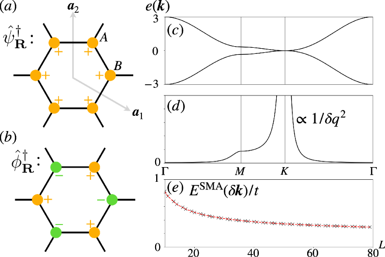
Figure 1: Frustration-free free-fermion model on the honeycomb. (a) Lattice convention and the definition of the local orbital corresponding to the conduction band. (b) Local orbital for the valence band. (c) Band structure. (d) Non-zero eigenvalue of the quantum metric tensor in arbitrary units, which diverges as $1/\delta q^{2}$ around the K point. (e) Excitation energy of density fluctuations within the single-mode approximation, which acquires an anomalous gap $O(1/\log L)$ due to the singular quantum metric. We take $\delta\bm{k}=(\bm{b}_{1}+\bm{b}_{2})/L$. Crosses are computed values and the dashed line indicates an inverse-log fit with fitting parameters reported in Appendix E.

Next, we turn to the finite-size excitation gap. The quadratic band touching immediately indicates that the single-particle excitation gap goes as $O(1/L^{2})$. Yet, it is also natural to ask if the charge-neutral excitation gap vanishes in the same way. The answer is again positive, as we can consider the particle-hole excitations in the band basis

$$\begin{split}|\bm{k},\bm{q}\rangle=\hat{f}^{\dagger}_{\bm{q}+\bm{k},c}\hat{f}_{\bm{q},v}|\Phi\rangle,\end{split}$$ (9)

where $|\Phi\rangle$ is the ground state, $\bm{k}$ labels the many-body momentum of the ansatz state, and the extra momentum $\bm{q}$ should be viewed as a label indicating the momentum of the created hole. Evidently, $|\bm{k},\bm{q}\rangle$ is an energy eigenstate of $\hat{H}$ with eigenvalue $t(e_{\bm{k}+\bm{q}}+e_{\bm{q}})$, and it disperses quadratically with $\bm{k}$ when $\bm{q}$ approaches K and K’. This shows that the charge-neutral excitation gap also vanishes as $O(1/L^{2})$.

Interaction and density fluctuations— Does the same excitation gap scaling hold beyond the non-interacting limit? For a general fermionic frustration-free model, we have shown in Ref. [53] that, assuming a power-law decay for a two-point correlation function in the ground state, the Gosset-Huang inequality [56] implies $\epsilon(L)\sim O((\log L)^{2}/L^{2})$. We now turn to validating this assertion when a local repulsion $\hat{U}=U\sum_{\bm{R}}(\hat{\psi}^{\dagger}_{\bm{R}}\hat{\psi}_{\bm{R}})(\hat{\phi}^{\dagger}_{\bm{R}}\hat{\phi}_{\bm{R}})$ with $U>0$ is added to the F⁴ model. By design, each local term in $\hat{U}$ is positive semi-definite and annihilates the non-interacting ground state $|\Phi\rangle$, and so $\hat{H}^{\rm int}=\hat{H}+\hat{U}$ remains a frustration-free Hamiltonian. Yet, $\hat{U}$ modifies the excitation energies although the ground states are unchanged, and so the behavior of $\epsilon(L)$ should be reexamined.

To bound $\epsilon(L)$, it suffices to consider suitable variational excited states. In the context of interacting frustration-free bosonic systems, this is often achieved through the density fluctuations treated within the single-mode approximation (SMA) [57]. The trial states take the form $|{\bm{k}}\rangle\propto\sum_{{\bm{R}}}\hat{n}_{\bm{R}}e^{i{\bm{k}}\cdot{\bm{R}}}|\Phi\rangle$, where $\hat{n}_{\bm{R}}$ is the total density operator in the unit cell ${\bm{R}}$. The SMA energy is given by the energy expectation value $E^{\rm SMA}({\bm{k}})=\langle{\bm{k}}|\hat{H}|{\bm{k}}\rangle/{\langle{\bm{k}}|{\bm{k}}\rangle}$, and corresponds to a quadratic gapless mode $E^{\rm SMA}({\bm{k}})\sim O(|{\bm{k}}|^{2})$ in many known models [58, 59, 60]. This quadratic dispersion again translates into a finite-size excitation gap $\epsilon(L)\sim O(1/L^{2})$, consistent with the bound obtained through the Gosset-Huang inequality [50].

Curiously, we now show that this commonly used ansatz does not provide a useful bound even in the free-fermion limit. Specifically, we show that $E^{\rm SMA}$ acquires an anomalous gap of $O(1/\log L)$ due to the diverging quantum metric in the F⁴ model. For definiteness, we take $|\Phi\rangle$ to be the state obtained by filling all the negative-energy modes. As a technical trick, we further assume a finite linear size $L$ which is not divisible by $3$. This avoids sampling the singular K and K’ points in the finite-size momentum mesh and leads to a unique ground state . The local density operator is given by $\hat{n}_{\bm{R}}=\sum_{\sigma=A,B}\hat{c}_{{\bm{R}},\sigma}^{\dagger}\hat{c}_{{\bm{R}},\sigma}$. In the momentum-space, for $\bm{k}\neq\bm{0}$ and using $\hat{f}_{\bm{q},c}|\Phi\rangle=\hat{f}_{\bm{q},v}^{\dagger}|\Phi\rangle=0$, we have

$$\begin{split}|{\bm{k}}\neq\bm{0}\rangle=\sum_{\bm{q}}F_{cv}(\bm{k},\bm{q})|\bm{k},\bm{q}\rangle,\end{split}$$ (10)

which can be viewed as a specific superposition of the excited states in Eq. (9). Here, $F_{cv}(\bm{k},\bm{q})$ is a form factor coming from the wave-function overlap $F_{cv}(\bm{k},\bm{q})=\bm{u}_{\bm{k+q},c}^{\dagger}\bm{u}_{\bm{q},v}$. The SMA energy for the F⁴ Hamiltonian is then obtained through the ratio between

$$\begin{split}\langle\bm{k}\neq\bm{0}|\hat{H}|\bm{k}\neq\bm{0}\rangle=&t\sum_{\bm{q}}\left|F_{cv}(\bm{k},\bm{q})\right|^{2}(e_{\bm{k+q}}+e_{\bm{q}});\\ \langle\bm{k}\neq\bm{0}|\bm{k}\neq\bm{0}\rangle=&\sum_{\bm{q}}\left|F_{cv}(\bm{k},\bm{q})\right|^{2}.\end{split}$$ (11)

As we are ultimately interested in the low-energy excitations, we may specialize to $\bm{k}\mapsto\delta\bm{k}$ with $|\delta\bm{k}|\rightarrow 0$, and then expand the form factor in this limit through $\bm{u}_{\bm{q}+\delta\bm{k},c}=\bm{u}_{\bm{q},c}+\sum_{i}\delta k_{i}\partial_{q_{i}}\bm{u}_{\bm{q},c}+O(\delta k^{2})$. As $\bm{u}_{\bm{q},c}^{\dagger}\bm{u}_{\bm{q},v}=0$, to leading order we have $\left|F_{cv}(\delta\bm{k},\bm{q})\right|^{2}=\sum_{i,j}\delta k_{i}\delta k_{j}g_{ij}(\bm{q})+O(\delta k^{3})$, where

$$\begin{split}g_{ij}(\bm{q})=\partial_{q_{i}}(\bm{u}_{\bm{q},c}^{\dagger})\bm{u}_{\bm{q},v}\bm{u}_{\bm{q},v}^{\dagger}\partial_{q_{j}}(\bm{u}_{\bm{q},c})\end{split}$$ (12)

is the quantum geometric tensor for the conduction band in the present two-band problem [62, 63, 64, 65]. Here, only the symmetric part of $g_{ij}(\bm{q})$, known as the quantum metric, contributes to $\left|F_{cv}(\delta\bm{k},\bm{q})\right|^{2}$.

Now, we notice that $\bm{u}_{\bm{q},\alpha}$ are not well-defined at the K and K’ points at which the two bands touch. At a momentum $\delta\bm{q}$ away from these singular points, the non-zero eigenvalue of the quantum metric diverges as $\sim 1/\delta q^{2}$ (Appendix C). When integrated, $\int d^{2}(\delta\bm{q})\,\delta q^{-2}$ diverges logarithmically with the low-momentum cutoff $1/L$. This then enters into the normalization factor in Eq. (11), which goes as $\langle\delta\bm{k}|\delta\bm{k}\rangle\sim\log(L)\delta k^{2}$. Although the divergence is cured in the numerator, which goes as $O(1)\delta k^{2}$, the SMA energy acquires an anomalous gap which vanishes logarithmically in the thermodynamic limit,

$$\begin{split}E^{\rm SMA}(\delta{\bm{k}})=\frac{\langle\delta\bm{k}|\hat{H}|\delta\bm{k}\rangle}{\langle\delta\bm{k}|\delta\bm{k}\rangle}\approx\frac{O(1)}{\log L}+\cdots.\end{split}$$ (13)

Therefore, in contrast to many gapless frustration-free bosonic models [58, 59, 60], we cannot conclude the asserted $O(1/L^{2})$ finite-size scaling through $E^{\rm SMA}(\bm{k})$.

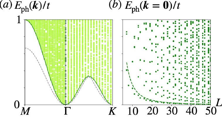
Figure 2: Energy of particle-hole excitations in $\hat{H}^{\rm int}$ at $U=2t$. (a) Energy spectrum of $\hat{H}^{\rm int}$ restricted into the subspace spanned by $|\bm{k},\bm{q}\rangle$ for $\bm{k}$ along the M-$\Gamma$-K line computed for $L=50$. The boundary of the particle-hole continuum can be estimated as $\min_{\bm{q}}(te_{\bm{q}}+(t+U)e_{\bm{q}+\bm{k}})$ (green solid line), which becomes exact in the non-interacting limit with $U=0$ (grey dashed line). Note that interaction $U>0$ modifies the excitation energies although it keeps the ground states unchanged. (b) System size dependence of the particle-hole energy at $\bm{k}=\bm{0}$. The dashed line shows the $O(1/L^{2})$ bound in Eq. (14).

Nevertheless, we can still demonstrate $\epsilon(L)\sim O(1/L^{2})$ using different variational excited states. In our fermionic context, another natural candidate is the zero-momentum particle-hole excitation $|\bm{0},\bm{q}\rangle$. In the free-fermion model, the smallest excitation energy is given by $\bm{q}$ in the vicinity of the K and K’ points, and it takes the form $2te_{\bm{q}_{L}}^{\rm min}$ with $e_{\bm{q}_{L}}^{\rm min}=\min\{e_{\bm{q}}>0\}\sim O(1/L^{2})$. As we show in Appendix D, a similar bound of $(2t+U)e_{\bm{q}_{L}}^{\rm min}$ can be derived when $U>0$. Analyzing $e_{\bm{q}_{L}}^{\rm min}$ further, we obtain

$$\begin{split}\epsilon(L)\leq(2t+U)2\pi^{2}\frac{1}{L^{2}}+O(1/L^{3})\end{split}$$ (14)

which provides the desired $O(1/L^{2})$ bound.

In Fig. 2, we show that the the particle-hole excitation indeed disperses quadratically around $\Gamma$, and verifies the discussed finite-size bound on the minimum excitation energy. Numerically, the bound of the charge-neutral finite-size gap using these ansatz states decay as $L^{-1.99(2)}$ (Appendix E), consistent with our analytical results.

Conclusions—In this work, we derived the necessary and sufficient conditions for local frustration-free free-fermion systems, and proved that the touching between conduction and valence bands in such model must be quadratic or softer. We also provided a concrete model on the honeycomb lattice, and found that the diverging quantum metric led to an anomalous gap in the density fluctuations. Nevertheless, one could construct charge-neutral excitations which bound the finite-size scaling of the excitation gap to be $O(1/L^{2})$ even in the presence of interaction, consistent with general results we obtained based on the ground-state correlation functions in an accompany work, Ref. [53].

Appendix A Details of the Dirac trick

Here, we explain why the Dirac trick applies to the full system even when the square root is apparently taken only for each of the local terms.

For concreteness, we focus on the original positive part of the F⁴ Hamiltonian, given by $\hat{H}^{(+)}=\sum_{\bm{R}}\sum_{\alpha=1}^{A_{\bm{R}}}\mu_{\bm{R}\alpha}\hat{\psi}_{\bm{R}\alpha}^{\dagger}\hat{\psi}_{\bm{R}\alpha}$. Define a compound index $\eta$ which runs over all of $\bm{R}$ and $\alpha$. Also, let $\hat{\bm{c}}^{\dagger}$ be a row vector containing all the fermion creation operators in the system. We may write the locally defined fermions as $\hat{\psi}_{\eta}^{\dagger}=\hat{\bm{c}}\bm{\psi}_{\eta}$. Here, $\bm{\psi}_{\eta}$ is a column vector which is mostly zero, as the corresponding fermion is localized around the unit cell $\bm{R}$ associated with $\eta$. With this notation, one has $\hat{H}^{(+)}=\hat{\bm{c}}^{\dagger}\left(\sum_{\eta}\bm{\psi}_{\eta}\mu_{\eta}\bm{\psi}_{\eta}^{\dagger}\right)\hat{\bm{c}}$. Let $Q$ be the matrix, generally not square, with the $\eta$-th column being $\bm{\psi}_{\eta}\sqrt{\mu_{\eta}}$. The single-particle Hamiltonian of $\hat{H}^{(+)}$ is given by $h^{(+)}=QQ^{\dagger}$. Noticing $\eta$ also indexes the auxiliary fermions introduced in the Dirac trick, one sees that

$$\begin{split}\tilde{h}^{(+)}=\left(\begin{array}[]{cc}0&Q\\ Q^{\dagger}&0\end{array}\right)\end{split}$$ (15)

when we combine all the local terms in defining the full-system single-particle matrix. Therefore, $(\tilde{h}^{(+)})^{2}$ contains $h^{(+)}$ as a block.

Appendix B Tight-binding form

Consider a chiral symmetric honeycomb model of spinless fermions. Let the nearest-neighbor hopping be $t_{1}$. Assuming chiral symmetry represented by $\sigma_{3}$ in the sublattice space, the next allowed hopping $t_{2}$ is between third nearest neighbors (Fig. 3). In momentum space, the Bloch Hamiltonian is given by $h_{\bm{k}}=Q_{\bm{k}}\sigma^{+}+Q_{\bm{k}}^{*}\sigma^{-}$, where

$$\begin{split}Q_{\bm{k}}=&t_{1}\left(1+e^{-i\bm{k}\cdot\bm{a}_{1}}+e^{i\bm{k}\cdot\bm{a}_{2}}\right)\\ &+t_{2}\left(e^{i\bm{k}\cdot(\bm{a}_{1}+\bm{a}_{2})}+e^{i\bm{k}\cdot(-\bm{a}_{1}+\bm{a}_{2})}+e^{-i\bm{k}\cdot(\bm{a}_{1}+\bm{a}_{2})}\right).\end{split}$$ (16)

One can verify that the F⁴ Hamiltonian defined in the main text gives the same model with $t_{1}=\frac{2}{3}t$ and $t_{2}=\frac{1}{3}t$. Conversely, the model is not F⁴ for other values of $t_{1}/t_{2}$.

For general ratios of $t_{1}/t_{2}$, the K and K’ points feature Dirac fermions. Expanding at the K point, we have

$$\begin{split}Q_{\bm{k}_{\rm K}+\delta\bm{k}}=\frac{\sqrt{3}}{2}e^{i5\pi/6}(t_{1}-2t_{2})(\delta k_{x}+i\delta k_{y})+O(\delta k^{2}).\end{split}$$ (17)

This implies the Dirac speed vanish at $t_{1}/t_{2}=2$, which is precisely the ratio realized in the F⁴ model.

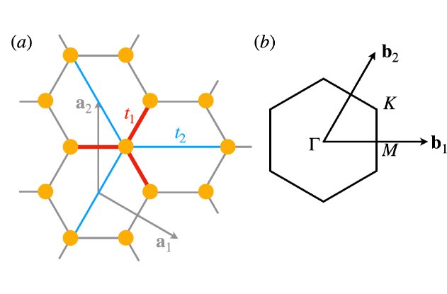
Figure 3: Spinless fermions on the honeycomb lattice. (a) The shortest bonds on the honeycomb lattice assuming a chiral symmetry forbidding intra-sublattice hopping. (b) Brillouin zone and special momenta.

Appendix C Quantum metric of the model and variational energy of density fluctuations

While the quantum metric is well-defined for isolated bands, it could become singular at band touching points. Indeed, in our F⁴ honeycomb model one finds $g_{ij}(\bm{q})\sim O(1/\delta q^{2})$ when $\bm{q}=\bm{q}_{\rm K}+\delta\bm{q}$ is around the K point (and similarly for the K’ point). More explicitly, we can parameterize $\bm{q}=\bm{q}_{K}+\delta q(\cos\theta,\sin\theta)$ and compute the leading singularity as

$$\begin{split}g_{\rm K}(\delta\bm{q})\approx\frac{1}{\delta q^{2}}\frac{3}{(2+\sin(2\theta))^{2}}\left(\begin{array}[]{cc}\sin^{2}(\theta)&-\sin\theta\cos\theta\\ -\sin\theta\cos\theta&\cos^{2}(\theta)\end{array}\right).\end{split}$$ (18)

One might notice that $g_{\rm K}(\delta\bm{q})$ has a $\theta$-dependent null vector for all values of $\theta$, but it does not play a role in our analysis.

We can now study how this singularity affects the SMA energy. For the energy expectation value in Eq. (11), the leading term in the $\delta k\rightarrow 0$ limit is given by $t\sum_{\bm{q}}(2e_{\bm{q}})g_{ij}(\bm{q})\delta k_{i}\delta k_{j}$. Since $e_{\bm{q}}\sim O(\delta q^{2})$ around the K and K’ points, the divergence in the quantum metric is compensated and one finds $\langle\delta\bm{k}|\hat{H}|\delta\bm{k}\rangle\sim O(1)\delta k^{2}$, agreeing with general results derived form a double-commutator bound assuming only the locality and charge conservation symmetry of $\hat{H}$ [57, 58, 59, 60]. In typical SMA calculations, the normalization factor starts at $O(1)$ and so the SMA energy is gapless and disperses quadratically.

For our model, however, the diverging quantum metric leads to a qualitatively different behavior for the SMA energy. The leading behavior of the normalization factor in Eq. (11) is given by $\left(\sum_{\bm{q}}g_{ij}(\bm{q})\right)\delta k_{i}\delta k_{j}$. The sum of $g_{ij}(\bm{q})$ over the Brillouin zone is dominated by the contribution from the K and K’ points, and its analytic behavior can be extracted by considering the integral

$$\begin{split}\int_{\frac{1}{L}}^{q_{0}}d\delta q\,\delta q\int_{0}^{2\pi}d\theta\,g_{\rm K}(\delta\bm{q})=\frac{2\pi}{\sqrt{3}}\log\left(q_{0}L\right)\left(\begin{array}[]{cc}1&\frac{1}{2}\\ \frac{1}{2}&1\end{array}\right),\end{split}$$ (19)

where we introduced a high-momentum cutoff of $q_{0}\sim O(1)$ and a low-momentum cutoff of $1/L$. Note that the matrix in Eq. (19) is positive definite, and so this leading order term is finite for all directions of $\delta\bm{k}$.

Therefore, although both the numerator and denominator in the SMA energy start with a quadratic term $\sim\delta k^{2}$, the coefficient for the numerator is $O(1)$ whereas that for the denominator is $O(\log L)$. This leads to $E^{\rm SMA}(\delta\bm{k})\sim O(1/\log L)$ in the limit $\delta k\rightarrow 0$, giving rise to an anomalous gap.

Appendix D Interacting bound of the neutral excitation gap

We first Fourier transform the interaction $\hat{U}$ to find

$$\begin{split}\hat{U}=\frac{U}{V}\sum_{\bm{q}_{1},\bm{q}_{2},\bm{p}}\sqrt{e_{\bm{q}_{2}-\bm{p}}e_{\bm{q}_{1}+\bm{p}}e_{\bm{q}_{2}}e_{\bm{q}_{1}}}\hat{f}^{\dagger}_{\bm{q}_{2}-\bm{p},c}\hat{f}_{\bm{q}_{2},c}\hat{f}^{\dagger}_{\bm{q}_{1}+\bm{p},v}\hat{f}_{\bm{q}_{1},v},\end{split}$$ (20)

where $V=L^{2}$ denotes the volume of the system. The quadratic term acts on the state $|\bm{k},\bm{q}\rangle$ to give

$$\begin{split}&\hat{f}^{\dagger}_{\bm{q}_{2}-\bm{p},c}\hat{f}_{\bm{q}_{2},c}\hat{f}^{\dagger}_{\bm{q}_{1}+\bm{p},v}\hat{f}_{\bm{q}_{1},v}|\bm{k},\bm{q}\rangle\\ =&\delta_{\bm{q}_{2},\bm{q}+\bm{k}}f^{\dagger}_{\bm{q}_{2}-\bm{p},c}\left(\delta_{\bm{p},\bm{0}}\hat{f}_{\bm{q},v}-\delta_{\bm{q}_{1}+\bm{p},\bm{q}}\hat{f}_{\bm{q}_{1},v}\right)|\Phi\rangle\\ =&\delta_{\bm{q}_{2},\bm{q}+\bm{k}}\delta_{\bm{p},\bm{0}}|\bm{k},\bm{q}\rangle-\delta_{\bm{q}_{2},\bm{q}+\bm{k}}\delta_{\bm{q}_{1}+\bm{p},\bm{q}}|\bm{k},\bm{q}-\bm{p}\rangle.\end{split}$$ (21)

We therefore obtain the matrix elements in the sector with many-body momentum $\bm{k}$ as

$$\begin{split}\langle\bm{k},\bm{q}^{\prime}|\hat{U}|\bm{k},\bm{q}\rangle=Ue_{\bm{q}+\bm{k}}\delta_{\bm{q}^{\prime},\bm{q}}-\frac{U}{V}\sqrt{e_{\bm{q}^{\prime}+\bm{k}}e_{\bm{q}+\bm{k}}e_{\bm{q}^{\prime}}e_{\bm{q}}}\end{split}$$ (22)

where we used $\sum_{\bm{q}_{1}}e_{\bm{q}_{1}}=V$ stemming from the F⁴ condition.

Next, we consider how the interaction modifies the charge-neutral excitation gap. While the particle-hole excitations $|\bm{k},\bm{q}\rangle$ are eigenstates of the free-fermion Hamiltonian, they become coupled when the interaction $\hat{U}$ is added to the Hamiltonian. As translation symmetry is preserved, sectors labeled by $\bm{k}$ remain decoupled. Let $\hat{H}^{\rm ph}|_{\bm{k}=\bm{0}}$ be the restriction of the Hamiltonian into the zero-momentum sector, defined by the matrix elements $\langle\bm{0},\bm{q}|\hat{H}^{\rm int}|\bm{0},\bm{q}^{\prime}\rangle$. Fig. 2(b) plots the low-lying eigenvalues of $\hat{H}^{\rm ph}|_{\bm{k}=\bm{0}}$ for different system sizes $L$. We can now find an upper bound to the smallest eigenvalue through

$$\begin{split}\min{\rm eig}\left(\hat{H}^{\rm ph}|_{\bm{k}=\bm{0}}\right)\leq&\min_{\bm{q}}\langle\bm{0},\bm{q}|\hat{H}^{\rm int}|\bm{0},\bm{q}\rangle\\ =&\min_{\bm{q}}\left(2te_{\bm{q}}+Ue_{\bm{q}}-\frac{U}{V}e_{\bm{q}}^{2}\right)\\ \leq&(2t+U)\min_{\bm{q}}e_{\bm{q}},\end{split}$$ (23)

where we used the matrix elements in Eq. (22) in the second line.

In our finite-size analysis, we take the linear size to be $L=3n+1$ or $L=3n+2$ with integer $n\geq 2$ such that we avoid sampling the K and K’ points. We parameterize $\bm{q}=\bm{q}_{\rm K}+\delta\bm{q}$ with $\delta\bm{q}=\delta q(\cos\theta,\sin\theta)$. For any fixed $\theta$, one can verify that $e_{\bm{q}_{\rm K}+\delta\bm{q}}$ increases monotonically with $0<\delta q\leq 1/7$. In the finite-size sampling of the BZ, there must be at least one sampled momentum within a distance of $1/L$ from the K point. We can therefore bound $\min_{\bm{q}}e_{\bm{q}}\leq\max_{\theta}e_{\bm{q}_{K}+(\cos\theta,\sin\theta)/L}$. In the vicinity of the K point, the single-particle dispersion is maximized at $\theta=5\pi/4$, and we may evaluate explicitly to find

$$\begin{split}\min_{\bm{q}}e_{\bm{q}}\leq&\eta\left(\delta q=\frac{1}{L}\right);\\ \eta(\delta q)=&4\sin^{2}\left(\frac{\pi\delta q}{\sqrt{2}}\right)\left[\cos\left(\frac{\pi\delta q}{\sqrt{2}}\right)+\frac{1}{\sqrt{3}}\sin\left(\frac{\pi\delta q}{\sqrt{2}}\right)\right]^{2}\\ =&2\pi^{2}\delta q^{2}+O(\delta q^{3}).\end{split}$$ (24)

Altogether, we obtain the bound

$$\begin{split}\min{\rm eig}\left(\hat{H}^{\rm ph}|_{\rm k=\bm{0}}\right)\leq&(2t+U)\eta\left(\frac{1}{L}\right),\end{split}$$ (25)

and the bound vanishes as $O(1/L^{2})$.

Appendix E Data analysis

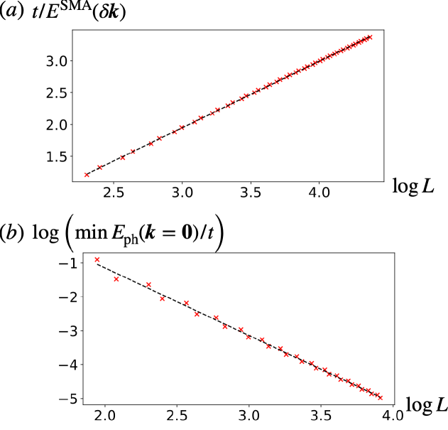
Figure 4: Fitting of numerical data. Red crosses indicated numerical data and dashed black lines are the linear fits. (a) The linear fit of $t/E^{\rm SMA}(\delta\bm{k})$ against $\log L$ gives a slope of $1.04(2)$ and an intercept of $-1.179(7)$. (b) The linear fit of the $\log$ of the minimum particle-hole excitation energy at $\bm{k}=\bm{0}$ against $\log L$ gives a slope of $-1.99(2)$ and an intercept of $2.84(8)$.