SCORE: Soft Label Compression-Centric Dataset Condensation via Coding Rate Optimization

Abstract

Dataset Condensation (DC) aims to obtain a condensed dataset that allows models trained on the condensed dataset to achieve performance comparable to those trained on the full dataset. Recent DC approaches increasingly focus on encoding knowledge into realistic images with soft labeling, for their scalability to ImageNet-scale datasets and strong capability of cross-domain generalization. However, this strong performance comes at a substantial storage cost which could significantly exceed the storage cost of the original dataset. We argue that the three key properties to alleviate this performance-storage dilemma are informativeness, discriminativeness, and compressibility of the condensed data. Towards this end, this paper proposes a Soft label compression-centric dataset condensation framework using COding RatE (SCORE). SCORE formulates dataset condensation as a min-max optimization problem, which aims to balance the three key properties from an information-theoretic perspective. In particular, we theoretically demonstrate that our coding rate-inspired objective function is submodular, and its optimization naturally enforces low-rank structure in the soft label set corresponding to each condensed data. Extensive experiments on large-scale datasets, including ImageNet-1K and Tiny-ImageNet, demonstrate that SCORE outperforms existing methods in most cases. Even with 30$\times$ compression of soft labels, performance decreases by only 5.5% and 2.7% for ImageNet-1K with IPC 10 and 50, respectively. Code will be released upon paper acceptance.

1 Introduction

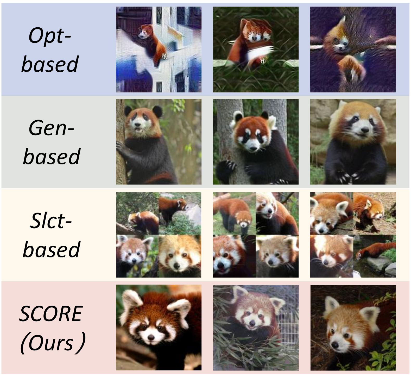
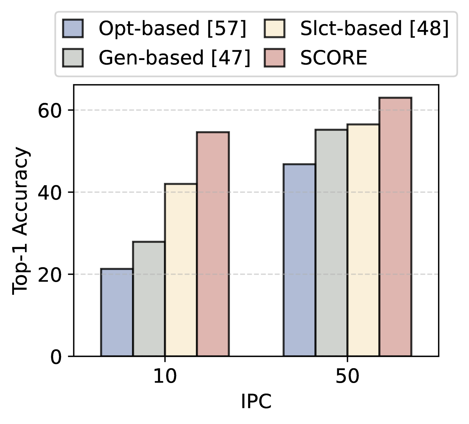
Figure 1: We compare the image quality and the corresponding model performance produced by four kinds of DC methods: Optimization-based, Generative model-based, Selection-based and Ours. Left: Visualization of different DC methods. Right: Performance comparison over different DC methods.

Dataset condensation (DC) [52] aims to compress a large-scale training dataset into a significantly smaller synthetic subset that can train downstream models with minimal loss in accuracy. Such condensation not only substantially reduces storage and computational requirements, but also enables flexible and customizable knowledge assembly for various downstream tasks. Prior DC approaches typically formulate dataset condensation as a pixel-level bi-level optimization problem, explicitly aligning training dynamics such as gradient trajectories [5, 21, 16, 10], data distribution [65, 51, 66], and parameter evolution [22, 31, 13] between synthetic samples and original sets. While effective on low-resolution benchmarks such as CIFAR [26] and MNIST [12], these approaches could barely scale to real-world, high-resolution datasets like ImageNet-1K. Key limitations include unaffordable memory consumption that scales quadratically with resolution and the limited realism of the yielded synthetic images, which often diverge far from the original data (1st row in Figure 1). The loss of realism arises from the overfitting of sythetic data to specific architectures used during optimization, severely restricting the generalization capacity across diverse downstream models. Consequently, recent studies prioritize enhancing sample realism by leveraging generative diffusion models [7, 47] (2nd row) to synthesize more high-fidelity images or directly selecting informative real samples [48] (3rd row) for ImageNet-scale condensation, leading to improved cross-architecture generalization.

While the visual realism is guaranteed in these approaches, they often sacrifice expressiveness required for effective training, as condensed samples inherently capture reduced intra- and inter-class variations as noted in [48]. To compensate for this expressiveness gap, recent works commonly employ fast knowledge distillation (FKD) [45], augmenting condensed samples with combined transformations such as RandomResizeCrop and CutMix [60] and generating the corresponding soft labels from the pretrained teacher models to transfer richer semantic knowledge.

Despite the benefits of soft labels, FKD-based strategies introduce substantial storage overhead, especially when the number of classes is large. For instance, DC approaches equipped with FKD [57, 43, 48] that condense ImageNet-1K [11] into 200 images per class would require approximately 200 GB for storing soft labels alone, which is almost twice the storage footprint of the full ImageNet-1K dataset. Recent efforts [41] have explored the random pruning of soft labels to mitigate this issue; however, blindly discarding label information is suboptimal, inevitably compromising the quality and richness of knowledge captured by the condensed dataset.

Motivated by this storage-performance dilemma, we introduce three fundamental criteria to guarantee realism and expressiveness in dataset condensation simultaneously: (1) Informativeness : selected samples should comprehensively capture the variability inherent in the original dataset; (2) Discriminativeness : condensed data should accurately represent class-specific discriminative information, facilitating downstream classification tasks; and (3) Compressibility : augmented soft labels should allow effective compression through rank-preserving techniques such as robust principal component analysis (RPCA), ensuring minimal information loss compared to naive random pruning. Inspired by these, we introduce SCORE, a Soft label compression-centric dataset condensation framework using COding RatE. Specifically, we unify these criteria within an information-theoretic min-max optimization framework centered around the concept of coding rate [36]. The coding rate theoretically serves as a concave surrogate for rank preservation that enables soft label compression. Notably, the coding rate exhibits a desirable submodular property, allowing us to divide and conquer the condensation process into an efficient greedy selection algorithm to balance realism, informativeness, and storage efficiency seamlessly. Extensive evaluations show that SCORE achieves state-of-the-art results across various datasets and network architectures under the same storage budget. Besides, SCORE empirically surpasses existing label compression approaches in DC, achieving improvements of up to 7.9% on Tiny-ImageNet and 20.3% on ImageNet-1K. Notably, SCORE reduces storage from 55.9 GB to only 1.9 GB on ImageNet-1K at 50 IPC, while maintaining 95.7% classification accuracy. The low-rank property induced by the coding rate in the condensed dataset ensures that the effectiveness of our compressed soft labels is agnostic to different compression strategies. By significantly reducing storage overhead while maintaining evaluation performance, SCORE provides a scalable and efficient solution for dataset condensation.

2 Related Work

2.1 Dataset Condensation

Dataset condensation (DC) aims to generate a compact yet informative dataset, enabling models to achieve performance comparable to training on the full dataset. This concept is first introduced by [52], which optimizes synthetic data by unrolling model training steps and matching model performance. While groundbreaking, their approach suffers from computationally inefficient bi-level optimization. The following researches propose surrogate objectives to overcome this limitation: distribution matching [65, 51, 66] aligns feature distributions using randomly initialized networks; gradient matching [63] and training trajectory [5, 62, 10, 16] matching ensures model parameter consistency by matching gradients across single or multiple training steps respectively. To generate synthetic images with higher resolution and greater realism, recent works [6, 64, 47, 39] exploit the power of generative models.

Most of these methods primarily optimize the images and only assign hard labels to the distilled images. However, soft labels in condensed datasets can even carry more information than synthetic images [41]. Therefore, SRe²L applies data augmentation to synthetic images, generating diverse soft labels for individual samples and achieving substantial performance gains over previous methods on ImageNet-scale datasets [11]. Building on the effectiveness of SRe²L, several dataset distillation methods [43, 47, 48, 14] have adopted this framework. Although soft labels can yield greater performance gains, their prohibitively large storage requirements contradict the fundamental goal of dataset condensation. In this work, we focus on constructing datasets with informativeness, discriminativeness and compressibility based on the principle of coding rate reduction.

2.2 Soft Label Compression

Soft labels improve model performance but demand significantly more storage, especially in SRe²L-like methods. Efficient compression is crucial to maintain their benefits while reducing storage costs. Since soft labels can be represented as matrices, existing matrix compression techniques, such as robust Principal Component Analysis (RPCA) [3] and Singular Value Decomposition (SVD), can decompose them into low-dimensional representations. Some methods exploit the intrinsic redundancy of soft labels, with Zipf’s Label Smoothing [28] using class rankings and FKD [45] retaining only top-$k$ soft scores. Beyond these approaches, Label Pruning for Large-scale Distillation (LPLD) [56] constructs a diverse label pool and randomly samples labels from it to reduce storage costs. However, the random selection process does not guarantee the retention of the most informative labels. In contrast, SCORE applies coding rate reduction, implemented via RPCA, to compress soft labels while preserving the most essential information, which ensures a higher degree of information retention and maintains model performance more effectively.

2.3 Coding Rate

In information theory, the rate distortion measures the minimum average number of bits required to encode data subject to a distortion level $\epsilon$. Due to the difficulty in computing rate distortion, coding rate serves as a practical alternative for its approximation [37]. Maximal Coding Rate Reduction (MCR²) [58] extends coding rate to facilitate the learning of diverse and discriminative feature representations. MCR² has been successfully applied to various tasks, including learning natural language representations [50], clustering images [19], and simplifying self-supervised learning pipelines [32]. Beyond these applications, coding rate has also been utilized to design interpretable deep networks and Transformer architectures, addressing the issue of catastrophic forgetting [8, 59, 55]. It has also demonstrated effectiveness in active learning by identifying the most informative samples [35]. Unlike previous works, we propose a unified criterion based on coding rate to construct a condensed dataset that meets three properties.

3 Critical Challenges in Dataset Condensation

3.1 Dataset Condensation

Dataset condensation (DC) addresses the fundamental challenge of condensing large-scale datasets into compact yet representative forms without significant loss of downstream accuracy. Consider an original dataset of $C$ classes $\mathcal{T}={\{{(\mathbf{x}}_{i},{\mathbf{y}}_{i})\}}^{|\mathcal{T}|}_{i=1}$, where $\mathbf{x}_{i}$ represents the $i$-th image and $\mathbf{y}_{i}$ its corresponding label. Recent DC methods utilize a teacher model $\phi_{h}(\cdot;\theta_{h})$ trained on $\mathcal{T}$ to generate a condensed dataset $\mathcal{S}$. This condensed dataset consists of synthetic images $\tilde{\mathcal{X}}$ and their associated soft labels. During training process of $K$ iterations, teacher model generates soft labels $\tilde{\mathcal{Y}}\in\mathbb{R}^{K\times C}$ for each image $\tilde{\mathbf{x}}\in\tilde{\mathcal{X}}$ based on various augmentations:

$$\tilde{\mathcal{Y}}=\{\tilde{\mathbf{y}}_{k}=\phi_{h}(A(\tilde{\mathbf{x}},k))\mid\tilde{\mathbf{x}}\in\mathcal{X}\}^{K}_{k=1},$$ (1)

where $A(\cdot,\cdot)$ represents the augmentation function. For a downstream student network $\phi(\cdot;\theta)$ trained on the condensed dataset, the objective is to minimize the Kullback-Leibler divergence between the model’s predictions and the teacher-generated soft labels across all samples in each iteration $k$:

$$\mathcal{L}(\mathcal{S},\theta)=\sum_{\tilde{\mathbf{x}}\in\mathcal{X}}\tilde{\mathbf{y}}_{k}\log\frac{\phi(A(\tilde{\mathbf{x}},k))}{\tilde{\mathbf{y}}_{k}}.$$ (2)

The keys of dataset condensation are twofold: (1) to achieve significant data compression, ensuring $|\mathcal{S}|\ll|\mathcal{T}|$, and (2) to maintain comparable model performance when training on $\mathcal{S}$ versus $\mathcal{T}$. This can be formulated as a bilevel optimization problem:

$$\mathcal{S}^{*}=\underset{\mathcal{S}}{\arg\min}\operatorname{\mathbb{E}}[\mathcal{L}(\mathcal{T},\theta_{\mathcal{S}})]~\text{s.t.}~\theta_{\mathcal{S}}=\underset{\theta}{\operatorname*{arg\,min}}\mathcal{L}(\mathcal{S},\theta).$$ (3)

3.2 Scaling Issues in DC

Storage Overhead. While current DC methods with soft labels are effective for large-scale datasets, concerns arise that soft labels overhead grows linearly with the number of classes $C$. Particularly for large-scale datasets such as ImageNet-1K, the storage requirements for soft labels can even exceed those of the condensed images themselves. For example, when obtaining a condensed dataset of ImageNet-1K with 50 image per class (IPC), its corresponding soft labels occupy nearly 56 GB while the images storage is only around 9 GB. Although common compression approaches such as RPCA can resolve the storage delimma, simply compressing soft labels results in severe information loss. As shown in Fig. 5, applying the same RPCA compression to soft labels from prior works leads to greater performance decline. When compressing soft labels to 5% of their original size, prior works suffer accuracy loss of up to 28.7%, whereas compression on our method maintains better performance, with only 16.1% performance drop.

Effectiveness of Dataset Synthesis. When condensing high-resolution datasets, the benefits of synthesizing images are questionable [48, 41]. The contribution of dataset synthesis is limited to evaluation performance. As illustrated in Fig. 1, optimization-based synthetic images fail to preserve realistic visual structures, making them less interpretable. Empirical results shown in bar plots (Fig. 1) demonstrate that DC methods using realistic images outperform those relying on synthetic images. Therefore, our work proposes dataset condensation based on selecting representative images from the original dataset, ensuring the preservation of realistic and crucial visual information. Based upon analysis of DC approaches, we identify three fundamental properties that characterize effective dataset condensation:

Proposition 1 (Fundamental properties of effective DC).

1. Informativeness: The condensed dataset must preserve and efficiently encode the essential information from the original dataset. This includes maximizing the information retention while minimizing the storage footprint.

2. Discriminativeness: To facilitate model classification, the condensed representation should keep clear discriminative boundaries between classes and capture the natural variations present in the original dataset.

3. Compressibility: The entire condensed representation, including both images and labels, must be storage-efficient. This property has been somewhat overlooked in previous works, which focus primarily on image compression while allowing label storage to grow unconstrained.

4 Methodology

Overview. SCORE employs a greedy selection algorithm to construct a condensed dataset that maintains both realism and essential characteristics of the original data. To reflect three properties, we design a unified goal using coding rate theory [36], and the algorithm (shown in Algorithm 1) iteratively builds the condensed dataset by selecting samples from the original dataset using Eq. 4. That is, the algorithm sequentially selects images until the budgets is reached. For each selection, it chooses the candidate sample $\mathbf{x}$ that yields highest Eq. 4, associated with its corresponding soft labels $\mathbf{Y}$ and the current selected image set $\mathcal{X}^{\prime}$:

$$\begin{split}R(\mathbf{x},\mathbf{Y}|\mathcal{X^{\prime}})&=\underbrace{R_{\operatorname{I}}(f(\{\mathbf{x}\}\cup\mathcal{X^{\prime}};\theta_{h}))}_{\text{{\color[rgb]{0.44921875,0.05859375,1}\leavevmode\resizebox{10.50002pt}{10.50002pt}{\includegraphics{figures/fire_blue.pdf}}}}}\\ &-\alpha\underbrace{R_{\operatorname{D}}(f(\{\mathbf{x}\}\cup\mathcal{X^{\prime}};\theta_{h}))}_{\text{{\color[rgb]{0.44921875,0.05859375,1}\leavevmode\resizebox{10.50002pt}{10.50002pt}{\includegraphics{figures/fire_green.pdf}}}}}-\beta\underbrace{R_{\operatorname{C}}(\mathbf{Y})}_{\text{{\color[rgb]{0.44921875,0.05859375,1}\leavevmode\resizebox{10.50002pt}{10.50002pt}{\includegraphics{figures/fire_purple.pdf}}}}},\end{split}$$ (4)

where $\alpha$ and $\beta$ are coefficients. The subsequent sections provide detailed analysis of each component in this unified criterion.

Informativeness through Coding Rate Theory. In the context of information theory [9], coding rate function $R_{\operatorname{I}}(\mathbf{Z})$ quantifies the minimum number of bits required to encode a feature space $\mathbf{Z}=[\mathbf{z}_{1},...,\mathbf{z}_{n}]\in\mathbb{R}^{d\times n}$ within a specified distortion tolerance [2] $\epsilon$:

$$R_{\operatorname{I}}(\mathbf{Z})=\frac{1}{2}\log\det\left(\mathbf{I}+\frac{d}{n{\epsilon}^{2}}\mathbf{Z}\mathbf{Z}^{\top}\right),$$ (5)

where $\mathbf{I}$ is the identity matrix and $d$ is the number of dimensions of feature $\mathbf{Z}$. In the context of dataset condensation, we aim to use minimum space to reflect maximal information of the original dataset. Therefore, our objective is to maximize the coding rate function $R_{\operatorname{I}}(\mathbf{Z})$, given that $\mathbf{Z}=f(\mathcal{X};\theta_{h})$ represents the features of condensed samples generated by pretrained model.

Enhanced Class Discriminability. For multi-class classification scenarios, where features naturally cluster into distinct subspaces, we extend the coding rate theory to incorporate class-aware information. Given a dataset with $C$ classes, we define the class-conditional coding rate as:

$$\mathcal{R}_{\operatorname{D}}(\mathbf{Z})=\sum_{j=1}^{C}\frac{\text{tr}(\Pi_{j})}{2n}\log\det\left(\mathbf{I}+\frac{d}{\text{tr}(\Pi_{j})\epsilon^{2}}\mathbf{Z}\Pi_{j}\mathbf{Z}^{\top}\right),$$ (6)

where $\Pi_{j}\in\mathbb{R}^{n\times n}$ is a diagonal matrix and the indices of samples that belong to the $j$-th class are set to be 1, 0 otherwise. This formulation computes the coding rates independently w.r.t. each class, thereby reflecting intra-class sample correlations. By minimizing this term, we promote the sparsification of features across different classes, thus enhancing discriminative power.

Soft Label Compressibility. We aim to reduce the storage overhead of soft labels by compressing the soft labels, while maintaining their effectiveness. Thus, to maintain the training accuracy with minimal sacrifice, we aim to encourage the soft labels of each image sample low-rank. The soft labels ${\mathbf{Y}}\in\mathbb{R}^{K\times C}$ for an image ${\mathbf{x}}$ are generated by the teacher model under various augmentations. We promote to select samples with low-rank structure in these soft labels by minimizing their coding rate:

$$\begin{split}R_{\operatorname{C}}({\mathbf{Y}})&=\frac{1}{2}\log\det\left(\mathbf{I}+\frac{d}{n{\epsilon}^{2}}\mathbf{Y}\mathbf{Y}^{\top}\right)\\ &\text{ s.t. }\mathbf{y}_{k}=\phi_{h}(A(\mathbf{x},k)).\end{split}$$ (7)

This term leverages the inherent approximate low-rank nature of soft labels, ensuring intra-class consistency while enabling effective compression.

5 Theoretical Analysis and Implementations

5.1 Why Coding Rate?

Coding Rate Exhibits Low-Rankness. One crucial objective of the work is to compress soft labels to reduce the storage overhead. To achieve effective compression, it is essential that soft labels exhibit low-rankness. If the soft labels of condensed samples possess low-rankness, information loss during compression is minimized.

Lemma 1 (Coding rate function is a concave surrogate for the rank function [15]).

For any matrix $\mathbf{Z}\in\mathbb{R}^{m\times n}$, coding rate function is strictly concave w.r.t. $\mathbf{Z}\mathbf{Z}^{\top}$ and provides a smooth approximation to the rank function.

In our framework, the coding rate function theoretically conforms to the objective of soft label compression. By minimizing the coding rate of soft labels through our unified objective in Eq. 4, we effectively minimize their rank, thereby enabling effective compression. The proof is shown in Supplementary.

Realistic Image Selection via Submodularity. Submodular functions indicate the information of a set in the context of information theoretics, which have been used in greedy subset selection methods [25, 24]. Submodular functions ensure that greedy algorithms select samples that align with optimal selection objectives [53]. A submodular function $f_{\operatorname{sub}}:2^{\Omega}\rightarrow\mathbb{R}$ on a finite set $\Omega$ satisfies the following condition: for any subsets $\mathcal{M}\subset\mathcal{N}\subseteq\Omega$ and element $\mathbf{x}\in\Omega\setminus{\mathcal{M}}$, the following inequality holds:

$$f_{\operatorname{sub}}(\mathcal{M}\cup{\{\mathbf{x}\}})-f_{\operatorname{sub}}(\mathcal{M})\geq f_{\operatorname{sub}}(\mathcal{N}\cup{\{\mathbf{x}\}})-f_{\operatorname{sub}}(\mathcal{N}).$$

The marginal gain in the submodular function value when adding an element $x$ to a selected set $\mathcal{X^{\prime}}$ is given by:

$$f_{\operatorname{sub}}(\mathbf{x}|\mathcal{X^{\prime}})=f_{\operatorname{sub}}(\{\mathbf{x}\}\cup\mathcal{X^{\prime}})-f_{\operatorname{sub}}(\mathcal{X^{\prime}}).$$ (8)

Lemma 2 (Coding rate function is submodular).

Given a set of features $\mathbf{Z}$ from a teacher model $\phi_{h}(\cdot;\theta_{h})$, coding rate function $R_{\operatorname{I}}(\mathbf{Z})$ satisfies the definition of submodular function.

This submodularity property ensures that our greedy selection algorithm achieves to maximize the coding rate-based objective. Each criterion of dataset condensation properties can be expressed as a conditional submodular function, measuring the marginal gain when adding an image sample to the condensed dataset.

Overall, by combining the marginal gains, we arrive at unified selection criterion in Eq. 4. The proof is provided in Supplementary and Algorithm 1 aims to select realistic samples with maximal scores w.r.t. Eq. 4.

5.2 Soft Label Compression

Since we find the intrinsic connection between coding rate theory and low-rankness, we perform low-rank compression for soft labels. Without loss of generality, we use the robust principle component (RPCA) analysis [3] to compress soft labels. Our strategy is also agnostic to varying compression methods, as demonstrated in Fig. 3. RPCA aims to decompose the soft label matrix $\mathbf{M}$ of a sample into a low-rank component $\mathbf{L}$ and a sparse matrix $\mathbf{S}$, forming a non-convex constraint problem:

$$\operatorname*{arg\,min}_{\mathbf{L},\mathbf{S}}rank(\mathbf{L})+\lambda\left\lVert\mathbf{S}\right\rVert_{0},\text{subject to }\mathbf{M}=\mathbf{L}+\mathbf{S},$$ (9)

where $\left\lVert\cdot\right\rVert_{0}$ is $\ell_{0}$ norm. We empirically adopt the Principle Component Pursuit (PCP) framework [3, 29, 30] to compress soft labels.

Algorithm 1 Maximal Coding Rate Dataset Condensation

Real Dataset $\mathcal{T}$; IPC; Teacher Network $\theta_{h}$

Subset $\mathcal{X}_{\text{select}}$

$\mathcal{X^{\prime}}\leftarrow\emptyset$ $\triangleright$ Initialize selected subset

$\mathcal{I^{\prime}}\leftarrow\emptyset$ $\triangleright$ Initialize selected indices

while $|\mathcal{X^{\prime}}|<\text{IPC}*C$ do

  $\mathcal{X}^{c}\leftarrow\text{Batch of candidate images from }\mathcal{T}\setminus\mathcal{X^{\prime}}$

  $j^{*}\leftarrow\operatorname*{arg\,max}_{j\notin\mathcal{I^{\prime}},\mathbf{x}_{j}\in\mathcal{X}^{c}}\mathcal{R}(\mathbf{x}_{j},\mathbf{Y}_{j}|\mathcal{X^{\prime}})$

  $\mathbf{X^{\prime}}\leftarrow\mathbf{X^{\prime}}\cup\{\mathbf{x}_{j^{*}}\}$

  $\mathcal{I^{\prime}}\leftarrow\mathcal{I^{\prime}}\cup\{j^{*}\}$

end while

return $\mathcal{X}_{\text{select}}$

6 Experiments

Dataset	IPC	MobileNet-V2		ResNet-18							ResNet-101
		EDC	SCORE	D4M [47]	SRE2L [57]	G-VBSM [43]	RDED [48]	LPLD [56]	EDC [44]	SCORE	SRE2L	RDED	EDC	SCORE
Tiny-ImageNet	10	40.6${\pm 0.6}$	48.8${\pm 0.1}$	-	33.1${\pm 0.4}$	-	41.9${\pm 0.2}$	35.2${\pm 0.2}$	51.2${\pm 0.5}$	51.3${\pm 0.2}$	33.9${\pm 0.6}$	22.9${\pm 3.3}$	51.6${\pm 0.2}$	50.8${\pm 1.1}$
	50	50.7${\pm 0.1}$	57.6${\pm 0.2}$	46.8${\pm 0.0}$	41.1${\pm 0.4}$	47.6${\pm 0.3}$	58.2${\pm 0.1}$	48.8${\pm 0.4}$	57.2${\pm 0.2}$	58.4${\pm 0.1}$	42.5${\pm 0.2}$	41.2${\pm 0.4}$	58.6${\pm 0.1}$	59.6${\pm 0.6}$
ImageNet-1K	10	45.0${\pm 0.2}$	49.3${\pm 0.3}$	27.9${\pm 0.0}$	21.3${\pm 0.6}$	31.4${\pm 0.5}$	42.0${\pm 0.1}$	34.6${\pm 0.9}$	48.6${\pm 0.3}$	54.6${\pm 0.2}$	30.9${\pm 0.1}$	48.3${\pm 1.0}$	51.7${\pm 0.3}$	62.5${\pm 0.3}$
	50	57.8${\pm 0.1}$	61.9${\pm 0.2}$	55.2${\pm 0.0}$	46.8${\pm 0.2}$	51.8${\pm 0.4}$	56.5${\pm 0.1}$	55.4${\pm 0.3}$	58.0${\pm 0.2}$	63.0${\pm 0.3}$	60.8${\pm 0.5}$	61.2${\pm 0.4}$	64.9${\pm 0.2}$	68.5${\pm 0.4}$

Table 1: Performance comparison of models trained on condensed Tiny-ImageNet and ImageNet-1K datasets, generated by using different dataset condensation techniques. All methods use an identical storage budget, and standard deviations are computed from three independent runs. The best-performing results are highlighted in red bold text, while the second-best results are marked with blue underlining.

Dataset	IPC	10$\times$				20$\times$				30$\times$
		SRe2L	RDED	LPLD	SCORE	SRe2L	RDED	LPLD	SCORE	SRe2L	RDED	LPLD	SCORE
Tiny-ImageNet	10	30.7${\pm 0.2}$‡	34.8${\pm 0.1}$‡	34.2${\pm 0.6}$‡	43.7${\pm 0.3}$	28.2${\pm 0.0}$‡	33.6${\pm 0.5}$‡	30.3${\pm 0.8}$‡	39.0${\pm 0.7}$	24.0${\pm 0.2}$‡	29.1${\pm 0.7}$‡	26.6${\pm 0.3}$‡	35.7${\pm 0.5}$
	50	40.3${\pm 0.0}$†	53.5${\pm 0.2}$‡	46.7${\pm 0.6}$†	55.5${\pm 0.1}$	39.0${\pm 0.0}$†	52.3${\pm 0.2}$‡	44.3${\pm 0.5}$†	53.4${\pm 0.3}$	34.6${\pm 0.0}$†	50.2${\pm 0.1}$‡	40.2${\pm 0.3}$†	49.9${\pm 0.2}$
ImageNet-1K	10	18.9${\pm 0.0}$†	36.9${\pm 0.6}$‡	32.7${\pm 0.6}$†	50.9${\pm 0.3}$	16.0${\pm 0.0}$†	33.8${\pm 0.1}$‡	28.6${\pm 0.4}$†	50.2${\pm 0.2}$	14.1${\pm 0.0}$†	28.8${\pm 0.3}$‡	23.1${\pm 0.1}$†	49.1${\pm 0.3}$
	50	44.1${\pm 0.0}$†	54.5${\pm 0.2}$‡	54.4${\pm 0.2}$†	60.8${\pm 0.2}$	41.5${\pm 0.0}$†	52.5${\pm 0.1}$‡	51.8${\pm 0.2}$†	60.4${\pm 0.5}$	37.2${\pm 0.0}$†	49.7${\pm 0.3}$‡	48.6${\pm 0.2}$†	60.3${\pm 0.4}$

Table 2: Performance comparison of ResNet-18 trained on condensed Tiny-ImageNet and ImageNet-1K datasets, generated by using different dataset condensation techniques. We reduce the storage budget of soft labels by 10$\times$, 20$\times$, 30$\times$ for each condensation method. The standard deviations are computed from three independent runs. ^†denotes the reported results, ^‡ denotes the reproduced results. The best-performing results are highlighted in red bold text, while the second-best results are marked with blue underlining.

In this section, we present a comprehensive experimental evaluation of our framework. First, we benchmark SCORE against state-of-the-art dataset condensation approaches. Next, we demonstrate the effectiveness of our soft label compression, which significantly reduces storage requirements while maintaining comparable model performance. Finally, we assess the cross-architecture generalization capability of the condensed dataset and investigate the contributions of individual components in our framework.

6.1 Experimental Setup

Datasets. To evaluate the effectiveness of SCORE, we conduct experiments on four large-scale datasets, including ImageNet-1K [11], Tiny-ImageNet [27], ImageWoof, and ImageNette [20]. ImageNet-1K consists of 1,281,167 training images spanning 1,000 categories, with a standard resolution of 256×256. ImageWoof and ImageNette are 10-class subsets of ImageNet-1K, maintaining the same resolution. Tiny-ImageNet is an ImageNet variant where images are resized to 64×64 pixels. Tiny-ImageNet contains 200 classes, with each class having 500 images.

Network Architectures. Following EDC [44], we use the full original dataset (i.e., ImageNet-1k, Tiny-ImageNet, etc.) and pretrained ResNet-18 [18] to select data and generate the corresponding soft labels. To demonstrate the strong cross-architecture generalization capacity, we leverage the ResNet-18 condensed data to train different mainstream network architectures, including ResNet-18 [18], ResNet-50 [18], ResNet-101 [18], MobileNet-V2 [42], EfficientNet-B0 [49], ConvNext-Tiny [34], ShffleNet-V2 [61], as well as Swin Transformer-Tiny [33]. All student models use the official implementation in torchvision [40], and will be trained from scratch.

Baselines. To validate the effectiveness of our proposed methods, we compare SCORE with a comprehensive set of recent state-of-the-art dataset condensation methods. Specifically, we compare with one generative model-based approach (i.e., D⁴M [47]), four optimization-basd approaches (i.e., SRE²L [57], G-VBSM [43], LPLD [56], and EDC [44]), and one selection-based method i.e., RDED [48]. D⁴M identifies optimal representative image embeddings through clustering techniques and subsequently utilize diffusion models to synthesize condensed images. Optimization-based methods refine synthetic images by aligning the statistical properties on the Batch Normalization layers between the original and condensed datasets. In contrast, RDED identifies and retains the most informative samples to construct a compact yet representative dataset.

6.2 Experimental Results

Benchmark Performance Evaluation. We compare SCORE with other dataset condensation approaches. Following previous works [57, 47, 43, 48, 44], we perform all experiments under the same storage budget to ensure a fair comparison. Additionally, to assess performance on smaller datasets, we conduct experiments on ImageWoof and ImageNette. The results for ImageNet-1K and Tiny-ImageNet are presented in Tab. 1, while those for ImageWoof and ImageNette are shown in Tab. 3. Across all datasets, our method consistently outperforms others with ResNet-18 and MobileNet V2 backbones, achieving significantly better results. In addition, with ResNet-101 backbone, it achieves performance on par with competing approaches, further demonstrating the effectiveness of our method. This superior performance stems from our dataset’s more realistic images, which offer better generalization capabilities across various network architectures and IPC settings. By optimizing our image selection criteria through maximizing $R_{\operatorname{I}}$ and minimizing $R_{\operatorname{D}}$ (Eq. 4), we ensure our condensed dataset retains both rich information content and high class discriminability, which directly translates to enhanced classification performance.

Performance with Compressed Soft Labels. To ensure the applicability of dataset condensation on the large-scale dataset, we evaluate how reduced soft label set affects the performances of the model trained on it.

Following [56], we compress the soft labels by factors of 10$\times$, 20$\times$ and 30$\times$. Compression is especially crucial for datasets with a larger number of classes and higher IPC values. Therefore, we conduct experiments on Tiny-ImageNet and ImageNet-1K with IPC values of 10 and 50. To assess the effectiveness of compressed datasets, we compare SCORE with LPLD [56], and we also apply LPLD’s compression method to SRe²L and RDED for further comparison. The experimental results are summarized in Tab. 2. Our method consistently outperforms or achieves comparable results across both datasets. On ImageNet-1K at 10 IPC, we surpass the second-best method, RDED, by 14.0%, 16.4%, and 20.3% under 10$\times$, 20$\times$, and 30$\times$ compression, respectively. At 50 IPC, the improvements are 6.3%, 7.9%, and 10.6%. This advantage arises from employing Eq. 4, which strategically selects samples that make soft labels more low-rank, ensuring strong performance even at high compression rates.

Cross-Architecture Generalization. To evaluate the generalizability of SCORE, we assess the condensed datasets across a variety of downstream models, including ResNet-18, ResNet-50, ResNet-101, MobileNet-V2, EfficientNet-B0, Swin-Tiny, ConvNext-Tiny, and ShuffleNet-V2. In these experiments, all student models are trained using ResNet-18 as the teacher model. To test the robustness of SCORE across different IPC settings, we consider a wider range of IPC values: 5, 10, 30, and 50. We compare our method with RDED and EDC, and as shown in Tab. 4, SCORE consistently outperforms both baselines across all models and IPC settings, with substantial improvements. These results highlight the versatility of our dataset for models of varying complexities. Notably, for lightweight models such as Swin-Tiny and ShuffleNet-V2 at lower IPC values, SCORE achieves performance improvements of 18.8%, 12.7%, 13%, and 17.4% over RDED and EDC, respectively. Our realistic images provide superior generalization and robustness across different downstream models while offering greater practical applicability. Furthermore, by leveraging coding rate optimization, SCORE selects samples with higher informativeness and discriminativeness, effectively addressing the limited expressiveness typically associated with real image subsets and significantly enhancing overall performance.

Dataset	IPC	ResNet-18			ResNet-101
		SRE2L	RDED	SCORE	SRE2L	RDED	SCORE
ImageWoof	10	30.0$\pm$0.8	44.4$\pm$1.8	45.1$\pm$1.7	22.3$\pm$0.7	35.9$\pm$2.1	42.5$\pm$0.9
	50	41.3$\pm$1.1	71.7$\pm$0.3	74.1$\pm$1.2	38.6$\pm$0.5	66.1$\pm$0.3	61.0$\pm$0.7
ImageNette	10	45.7$\pm$1.0	62.7$\pm$0.8	71.6$\pm$0.2	36.1$\pm$2.5	53.3$\pm$2.7	63.9$\pm$1.2
	50	64.4$\pm$0.7	84.4$\pm$0.2	84.5$\pm$0.2	62.8$\pm$0.4	80.9$\pm$0.4	81.3$\pm$1.4

Table 3: Performance comparison of models trained on different condensed ImageWoof and ImageNette datasets. All methods use an identical storage budget, and standard deviations are computed from three independent runs. The best-performing results are highlighted in red bold text, while the second-best results are marked with blue underlining.

IPC	Method	ResNet-18	ResNet-50	ResNet-101	MobileNet-V2	EfficientNet-B0	Swin-Tiny	ConvNext-Tiny	ShuffleNet-V2
5	RDED [48]	30.5	36.0	35.5	21.9	28.1	12.4	25.9	20.1
	EDC [44]	36.6	40.6	41.0	31.8	39.2	18.5	33.9	15.7
	SCORE	39.4	41.8	48.9	36.9	46.1	31.2	42.8	33.1
10	RDED [48]	42.0	46.0	48.3	34.4	42.8	29.2	48.3	19.4
	EDC [44]	48.6	54.1	51.7	45.0	51.1	38.3	54.4	29.8
	SCORE	54.6	60.2	62.5	49.3	58.5	49.2	63	37.4
30	RDED [48]	49.9	59.4	58.1	44.9	54.1	47.7	62.1	23.5
	EDC [44]	55.0	61.5	60.3	53.8	58.4	59.1	63.9	41.1
	SCORE	61.3	66.8	67.3	59.6	63.1	64.5	68.1	54.8
50	RDED [48]	56.5	63.7	61.2	53.9	57.6	56.9	65.4	30.9
	EDC [44]	58.0	64.3	64.9	57.8	60.9	63.3	66.6	45.7
	SCORE	63.0	68.4	68.5	61.8	65.9	67.2	69.6	57.8

Table 4: Cross-architecture generalization performance on ImageNet-1K.

6.3 Further Analysis

Hyper-parameter Sensitivity Analysis. We conduct a sensitivity analysis on the hyper-parameters in Eq. 4, specifically the coefficients $\alpha$ and $\beta$ of the terms $R_{\operatorname{D}}(\mathbf{Z})$ and $R_{\operatorname{C}}({\mathbf{Y}})$. These coefficients control the balance between Discriminativeness and Compressibility. Theoretically, when $\beta$ is larger, the soft labels of the data tend to experience less information loss during compression. To examine the impact of coefficients individually, we fix $\alpha$ to 5 and vary $\beta$ across the values 0.5, 1, 3, 5, and 10. Additionally, $\beta$ is fixed at 0.5 while $\alpha$ is varied over the same range. Experiments are conducted on ImageNet-1K, with soft label storage compressed to align with the 300-epoch storage budget. Using ResNet-18 as the backbone, we evaluate performance under the 10 IPC setting. As shown in the Fig. 4, the classification results are sensitive to the choice of $\alpha$ (red dashed line), with the best performance achieved when $\alpha=3$, which is approximately 1.5% better than the worst result at $\alpha=10$. The effect of different $\beta$ values on the results is relatively steady. Generally, as $\beta$ increases, the performance after compression tends to improve.

Coreset and Active Learning Method Analysis. To assess the effectiveness of selection based on the maximal coding rate criterion, we compare SCORE against various coreset selection strategies on ImageWoof at 10 IPC. The baselines include random selection, Herding [54], Bait [38], GradMatch [21], and BADGE [1], an active learning variant that utilizes a pretrained model instead of iterative training. All methods use the same evaluation pipeline with the same storage budget. As shown in Fig. 2, SCORE significantly outperforms the alternatives, demonstrating that the dataset constructed using $R_{\operatorname{I}}$ and $R_{\operatorname{D}}$ in the unified criterion Eq. 4 preserves more information from the original dataset and exhibits better discriminativeness.

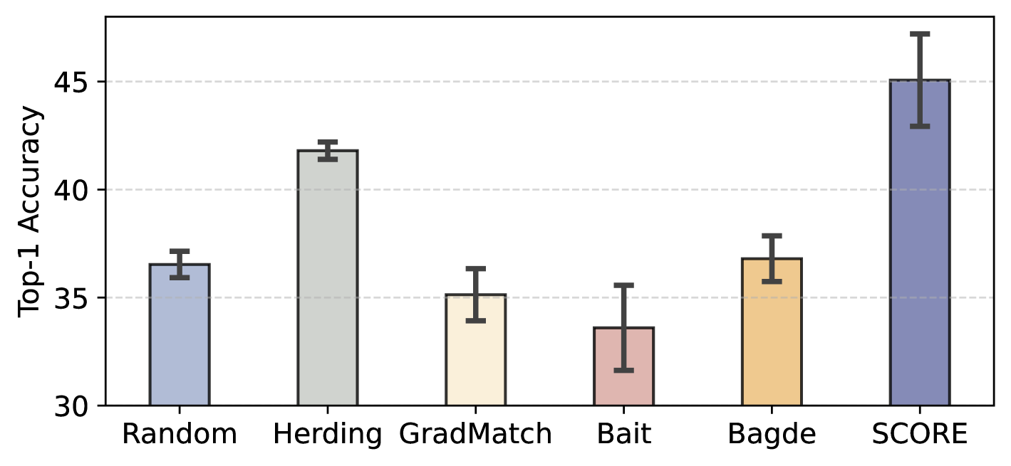
Figure 2: The comparison among various coreset selection methods on ImageWoof with IPC=10.

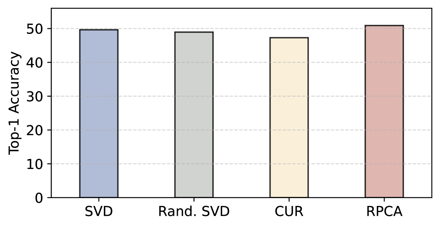
Figure 3: The comparison among soft label compression methods on ImageNet-1K with IPC=10.

Sensitivity to Label Compression Choices. We evaluate the compressibility of our condensed dataset using various low-rank compression techniques, including SVD [23], Randomized SVD [17], CUR [46], and RPCA [4], on ImageNet-1K at 10 IPC. Figure 3 shows that SCORE exhibits good stability across different compression methods. These results substantiate our original hypothesis: if the soft label set of a condensed dataset inherently exhibits a low-rank structure, it becomes particularly amenable to low-rank compression techniques with minimal information loss. Furthermore, the performance discrepancy observed between the highest-performing method (RPCA) and the lowest-performing alternative is approximately 3.5%. This relatively minor gap underscores the robustness of our approach in generating soft labels with reliably low-rank characteristics. Considering its superior performance in our comparative analysis, we selected RPCA as the principal compression method for subsequent experiments.

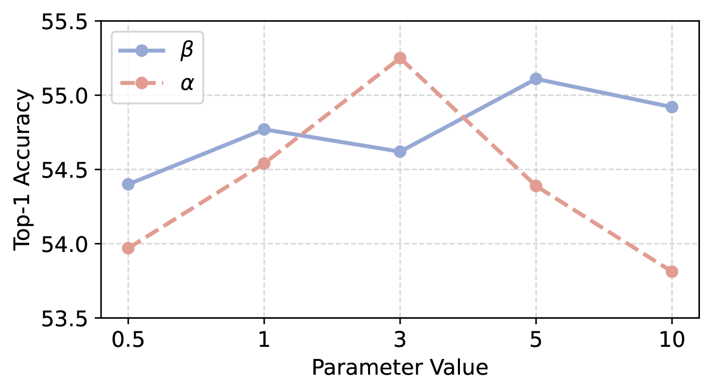
Figure 4: Parameter sensitivity analysis of $\alpha$ and $\beta$ in Eq. 4.

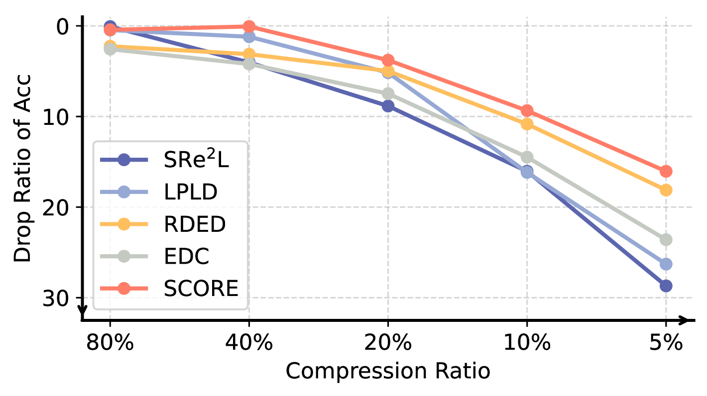
Figure 5: The performance drop comparison across different methods.

Resilience to Soft Label Compression. To demonstrate the advantage of our image selection framework in facilitating soft label compression, we apply RPCA to the soft label set of condensed ImageNet-1K generated by various methods, including SRe²L, RDED, LPLD, EDC, at 10 IPC and train ResNet-18 on the compressed data. Specifically, we establish 300 epochs as the baseline and progressively compress these datasets to 5%, 10%, 20%, 40%, and 80% of the original storage. All methods are evaluated under the same training pipeline. As shown in Fig. 5, besides demonstrating superior performance before compression, SCORE consistently experiences a smaller performance degradation across all compression rates compared to other methods. This observation suggests that optimizing the Compressibility term, $R_{\operatorname{C}}({\mathbf{Y}})$, significantly contributes to stabilizing the variability of soft labels derived from data augmentation. Thus, our selection criterion produces datasets with enhanced resilience to information loss during compression, highlighting the strong potential of our approach to significantly reduce storage requirements while maintaining robust model performance.

7 Conclusion

In this study, we addressed the soft label storage overhead challenge of dataset condensation for large scale datasets. We identified three fundamental properties essential for dataset condensation: informativeness, discriminativeness and compressibility. Based on these principles, we proposed SCORE, a dataset condensation method that reduces soft label overhead while maintaining performance. We designed a unified criterion using code rate theory to select realistic images for constructing condensed dataset. SCORE employs RPCA for low-rank soft label compression, while minimizing information loss through our dataset condensation objectives. Experimental results demonstrate that our condensed datasets consistently outperform those from existing methods in downstream model evaluation. The unified selection criterion enables the condensed datasets with informative samples, higher soft label compression ratios and minimal information loss, thereby enhancing the practicality of dataset condensation.

This supplementary material provides additional descriptions of proposed dataset condensation method SCORE, including theoretical proofs and empirical details. Visualizations of condensed datasets are demonstrated to enhance understanding of the proposed method.

• Sec. 8.1: Proof of Coding Rate for Rank Approximation.

• Sec. 8.2: Proof of Coding Rate Submodularity.

• Sec. 9: Unified Criterion Derivation.

• Sec. 10: Hyper-Parameter Settings.

• Sec. 11: Visualizations.

8 Proof

8.1 Proof of Lemma 1

Log-det is justified as a smooth approximation for the rank function [15]. For any matrix $\mathbf{Z}\in\mathbb{R}^{m\times n}$, coding rate function is strictly concave w.r.t. $\mathbf{Z}\mathbf{Z}^{\top}$ and provides a smooth approximation to the rank function.

Proof.

For all vectors $\mathbf{x}$, given a coefficient $\lambda$ and feature matrix $\mathbf{Z}$, we have

$$\begin{split}\mathbf{x}^{\top}(\mathbf{I}+\lambda\mathbf{Z}\mathbf{Z}^{\top})\mathbf{x}&=\mathbf{x}^{\top}\mathbf{I}\mathbf{x}+\lambda\mathbf{x}^{\top}\mathbf{Z}\mathbf{Z}^{\top}\mathbf{x}\\ &=\mathbf{x}^{\top}\mathbf{x}+\lambda\mathbf{x}^{\top}\mathbf{Z}^{\top}\mathbf{Z}\mathbf{x}\\ &={\lVert{\mathbf{x}}\rVert}^{2}+\lambda{\lVert{\mathbf{Z}^{\top}\mathbf{x}}\rVert}^{2}\\ &\geq 0.\end{split}$$ (10)

Therefore, the term $\mathbf{I}+\lambda\mathbf{Z}\mathbf{Z}^{\top}$ is positive semidefinite. Now let $\mathbf{Z}\mathbf{Z}^{\top}=\mathbf{M}$. Assume $\mathbf{M}_{1}$ and $\mathbf{M}_{2}$ be positive semidefinite matrices, and let $0\leq\alpha\leq 1$. Define:

$$X_{1} =\mathbf{I}+\lambda\mathbf{M}_{1},$$

$$X_{2} =\mathbf{I}+\lambda\mathbf{M}_{2}.$$

For any convex combination:

$$\alpha X_{1}+(1-\alpha)X_{2} =\alpha(\mathbf{I}+\lambda\mathbf{M}_{1})+(1-\alpha)(\mathbf{I}+\lambda\mathbf{M}_{2})$$ (11)

$$=\mathbf{I}+\lambda(\alpha\mathbf{M}_{1}+(1-\alpha)\mathbf{M}_{2}).$$ (12)

$\log\det(X)$ is concave on the set of positive definite matrices. Therefore:

$$\log\det(\alpha X_{1}+(1-\alpha)X_{2})\geq\alpha\log\det(X_{1})+(1-\alpha)\log\det(X_{2})$$ (13)

Substituting to the definitions:

$$\log\det(\mathbf{I}+\lambda(\alpha\mathbf{M}_{1}+(1-\alpha)\mathbf{M}_{2}))\geq\alpha\log\det(\mathbf{I}+\lambda\mathbf{M}_{1})+(1-\alpha)\log\det(\mathbf{I}+\lambda\mathbf{M}_{2}).$$ (14)

This confirms that $f(\mathbf{M})=\log\det(\mathbf{I}+\lambda\mathbf{M})$ is concave in $\mathbf{M}$.

Let $\mathbf{M}$ have eigenvalues $\mu_{1},\mu_{2},\ldots,\mu_{n}$ (all non-negative since $\mathbf{M}$ is positive semidefinite).

Then $\mathbf{I}+\lambda\mathbf{M}$ has eigenvalues $1+\lambda\mu_{1},1+\lambda\mu_{2},\ldots,1+\lambda\mu_{n}$.

The determinant is the product of eigenvalues, so:

$$\det(\mathbf{I}+\lambda\mathbf{M})=\prod_{i=1}^{n}(1+\lambda\mu_{i})$$ (15)

Taking the logarithm:

$$\log\det(\mathbf{I}+\lambda\mathbf{M})=\sum_{i=1}^{n}\log(1+\lambda\mu_{i})$$ (16)

Now, as $\lambda\to\infty$:

• For $\mu_{i}>0$: $\log(1+\lambda\mu_{i})\approx\log(\lambda\mu_{i})=\log(\lambda)+\log(\mu_{i})$

• For $\mu_{i}=0$: $\log(1+\lambda\mu_{i})=\log(1)=0$

Let $r=rank(\mathbf{M})$, which is the number of positive eigenvalues. For a non-zero $\lambda$, we have:

$$\log\det(\mathbf{I}+\lambda\mathbf{M}) \approx\sum_{i:\mu_{i}>0}\log(\lambda\mu_{i})$$ (17)

$$=\sum_{i:\mu_{i}>0}\log(\lambda)+\sum_{i:\mu_{i}>0}\log(\mu_{i})$$ (18)

$$=r\log(\lambda)+\sum_{i:\mu_{i}>0}\log(\mu_{i})$$ (19)

Thus, $\log\det(\mathbf{I}+\lambda\mathbf{M})\approx r\log(\lambda)+c$, where $c=\sum_{i:\mu_{i}>0}\log(\mu_{i})$ is a constant that depends on the non-zero eigenvalues of $\mathbf{M}$.

This shows that for large $\lambda$, minimizing $\log\det(\mathbf{I}+\lambda\mathbf{M})$ is approximately equivalent to minimizing the rank of $\mathbf{M}$, up to scaling by $\log(\lambda)$ and an additive constant.

∎

8.2 Proof of Lemma 2

Given a set of features $\mathbf{Z}$, coding rate function $R_{\operatorname{I}}(\mathbf{Z})=\log\det(\mathbf{I}+\lambda\mathbf{Z}\mathbf{Z}^{\top})$ satisfies the definition of submodular function. To prove submodularity, $R_{\operatorname{IC}}$ should satisfy diminishing returns property: for any sets $\mathcal{A}\subseteq\mathcal{B}$ and any element $i\notin\mathcal{B}$, if a function $f$ is submodular, we have $f(\mathcal{A}\cup\{i\})-f(\mathcal{A})\geq f(\mathcal{B}\cup\{i\})-f(\mathcal{B})$. Let $\mathcal{A}\subseteq\mathcal{B}$ be two sets of indices for $\mathbf{Z}$, we need to show:

$$R_{\operatorname{I}}(\mathbf{Z}_{\mathcal{A}\cup\{i\}})-R_{\operatorname{I}}(\mathbf{Z}_{\mathcal{A}})\geq R_{\operatorname{I}}(\mathbf{Z}_{\mathcal{B}\cup\{i\}})-R_{\operatorname{I}}(\mathbf{Z}_{\mathcal{B}}).$$ (20)

Proof.

Given a set $\mathcal{S}$, we can rewrite the term using matrix determinant lemma:

$$\begin{split}R_{\operatorname{IC}}(\mathbf{Z}_{\mathcal{S}}\cup\{i\})-R_{\operatorname{IC}}(\mathbf{Z}_{\mathcal{s}})&=\log{\det(\mathbf{I}+\lambda\mathbf{Z}_{\mathcal{S}\cup\{i\}}\mathbf{Z}^{\top}_{\mathcal{S}\cup{\{i\}}})}-\log\det(\mathbf{I}+\lambda\mathbf{Z}_{\mathcal{S}}\mathbf{Z}^{\top}_{\mathcal{S}})\\ &=\log{\frac{\det(\mathbf{I}+\lambda\mathbf{Z}_{\mathcal{S}\cup\{i\}}\mathbf{Z}^{\top}_{\mathcal{S}\cup{\{i\}}})}{\det(\mathbf{I}+\lambda\mathbf{Z}_{\mathcal{S}}\mathbf{Z}^{\top}_{\mathcal{S}})}}\\ &=\log(1+\lambda\mathbf{z}_{i}^{\top}(\mathbf{I}+\lambda\mathbf{Z}_{\mathcal{S}}\mathbf{Z}_{\mathcal{S}}^{\top})^{-1}\mathbf{z}_{i}).\end{split}$$ (21)

Since $\mathcal{A}\subseteq\mathcal{B}$, thus $\mathbf{Z}_{\mathcal{A}}\mathbf{Z}_{\mathcal{A}}^{\top}$ is a principle submatrix of $\mathbf{Z}_{\mathcal{B}}\mathbf{Z}_{\mathcal{B}}^{\top}$, thus we have:

$$\mathbf{Z}_{\mathcal{B}}\mathbf{Z}_{\mathcal{B}}^{\top}-\mathbf{Z}_{\mathcal{A}}\mathbf{Z}_{\mathcal{A}}^{\top}\succeq 0,$$ (22)

where $\succeq$ denotes the Löwner partial order. Using matrix inversion lemma, we can show that:

$${(\mathbf{I}+\lambda\mathbf{Z}_{\mathcal{A}}\mathbf{Z}_{\mathcal{A}}^{\top})}^{-1}-{(\mathbf{I}+\lambda\mathbf{Z}_{\mathcal{B}}\mathbf{Z}_{\mathcal{B}}^{\top})}^{-1} \succeq 0$$

$$\mathbf{z}_{i}^{\top}[{(\mathbf{I}+\lambda\mathbf{Z}_{\mathcal{A}}\mathbf{Z}_{\mathcal{A}}^{\top})}^{-1}-{(\mathbf{I}+\lambda\mathbf{Z}_{\mathcal{B}}\mathbf{Z}_{\mathcal{B}}^{\top})}^{-1}]\mathbf{z}_{i} \geq 0.$$

Therefore, $R_{\operatorname{I}}(\mathbf{Z}_{\mathcal{s}}\cup\{i\})-R_{\operatorname{I}}(\mathbf{Z}_{\mathcal{s}})$ is monotonically decreasing, which proves that: given $\mathcal{A}\subseteq\mathcal{B}$, the inequality holds:

$$R_{\operatorname{I}}(\mathbf{Z}_{\mathcal{A}}\cup\{i\})-R_{\operatorname{I}}(\mathbf{Z}_{\mathcal{A}})\geq R_{\operatorname{I}}(\mathbf{Z}_{\mathcal{B}}\cup\{i\})-R_{\operatorname{I}}(\mathbf{Z}_{\mathcal{B}}),$$ (23)

and $R_{\operatorname{I}}$ is a submodular function. ∎

9 Derivation for Unified Criterion

In the image selection process, we aim to select samples that maximize the marginal gain of the unified criterion in each round. For a selected set $\mathcal{S}$, when a function $f_{\operatorname{sub}}$ is submodular, the marginal gain of adding element $i$ to $\mathcal{S}$ is defined as:

$$f_{\operatorname{sub}}(\{i\}|\mathcal{S})=f_{\operatorname{sub}}(\mathcal{S}\cup\{i\})-f_{\operatorname{sub}}(\mathcal{S}).$$ (24)

Based on this submodularity property, given that certain terms remain constant during a single selection iteration, the optimal image $\mathbf{x}^{*}$ can be determined as follows:

$$\begin{split}x^{*}&=\underset{x}{\arg\max}R(\mathbf{x},\mathbf{Y}|\mathcal{X}^{\prime})\\ &=\underset{x}{\arg\max}R_{\operatorname{I}}(f(\{\mathbf{x}\}\cup\mathcal{X}^{\prime};\theta_{h}))-R_{\operatorname{I}}(f(\mathcal{X}^{\prime};\theta_{h}))\\ &\quad-\alpha R_{\operatorname{D}}(f(\{\mathbf{x}\}\cup\mathcal{X}^{\prime};\theta_{h}))+\alpha R_{\operatorname{D}}(f(\mathcal{X}^{\prime};\theta_{h}))-\beta R_{\operatorname{C}}(\mathbf{Y})\\ &=\underset{x}{\arg\max}R_{\operatorname{I}}(f(\{\mathbf{x}\}\cup\mathcal{X}^{\prime};\theta_{h}))-\alpha R_{\operatorname{D}}(f(\{\mathbf{x}\}\cup\mathcal{X}^{\prime};\theta_{h}))-\beta R_{\operatorname{C}}(\mathbf{Y}).\end{split}$$ (25)

10 Hyper-Parameter Settings

All experiments utilize the AdamW optimizer for model training and apply RandomResizeCrop, RandomHorizontalFlip, and cutmix as data augmentations. The specific hyperparameter settings for all datasets are detailed in Tab. 5. These include the values of $\alpha$ and $\beta$ used for image selection, the minimum and maximum scales for the RandomResizeCrop augmentation, as well as other network parameters such as learning rate, weight decay, temperature $T$, batch size, and the number of training epochs.

Table 5: Hyper-parameter on the ImageNet-1K, Tiny-ImageNet, ImageWoof and ImageNette.

	ImageNet-1K		Tiny-ImageNet		ImageWoof		ImageNette
	IPC		IPC		IPC		IPC
Hyper-parameter	10	50	10	50	10	50	10	50
$\alpha$	5	5	5	10	5	5	0.1	0.1
$\beta$	1	1	0.001	0.001	0.1	0.1	0.1	0.1
Min scale of Aug	0.4	0.4	0.3	0.4	0.3	0.3	0.2	0.2
Max scale of Aug	1	1	1	1	1	1	1	1
Learning Rate	0.001	0.001	0.001	0.001	0.001	0.001	0.0005	0.0005
Weight Decay	0.01	0.01	0.01	0.01	0.01	0.01	0.01	0.01
$T$	20	20	20	20	20	20	10	10
Batch Size	64	64	50	50	64	64	10	10

11 Visualization

The visualizations of our selected images, presented in Figs. 6, 7, 8 and 9, are randomly sampled from the condensed datasets of ImageNet-1K, Tiny ImageNet, ImageWoof, and ImageNette, respectively.

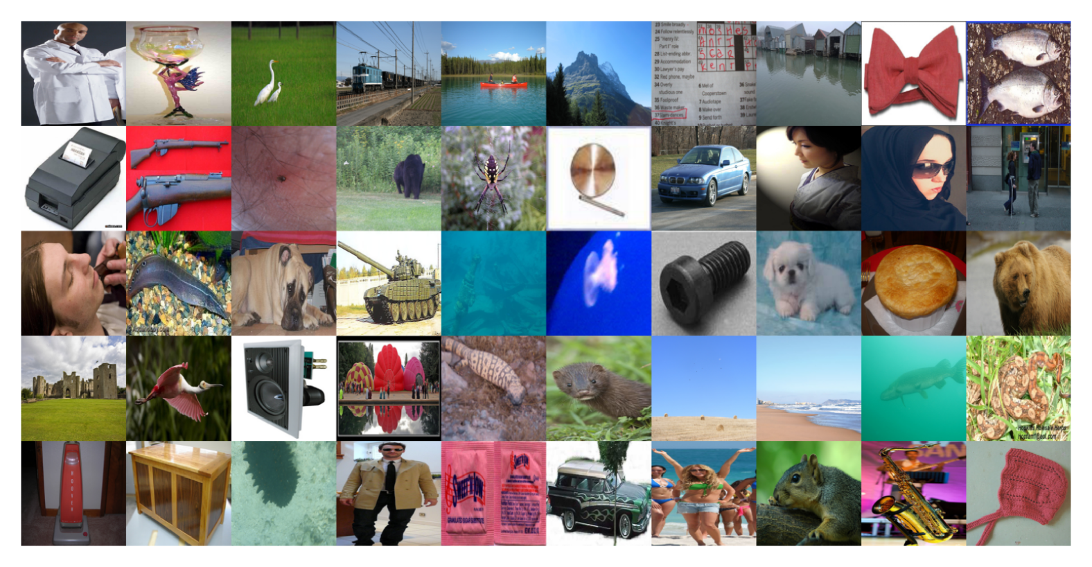
Figure 6: visualization of the condensed ImageNet-1k.

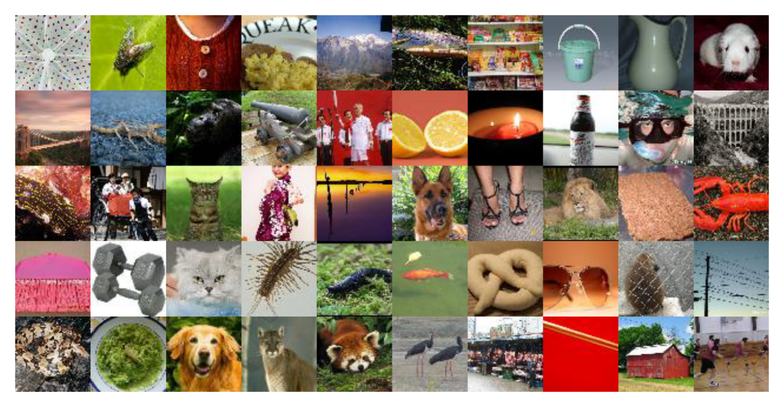
Figure 7: visualization of the condensed Tiny-ImageNet.

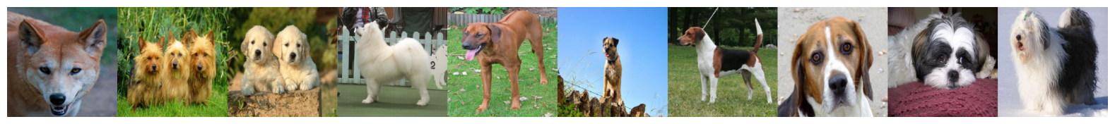
Figure 8: visualization of the condensed ImageWoof.

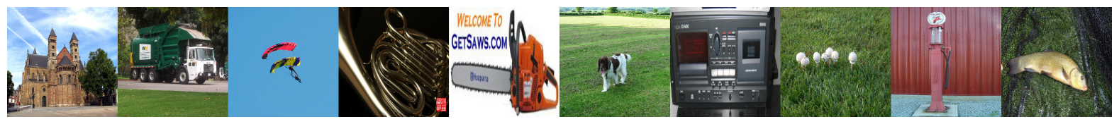
Figure 9: visualization of the condensed ImageNette.

References

- Ash et al. [2020] Jordan T. Ash, Chicheng Zhang, Akshay Krishnamurthy, John Langford, and Alekh Agarwal. Deep batch active learning by diverse, uncertain gradient lower bounds. In 8th International Conference on Learning Representations, ICLR 2020, Addis Ababa, Ethiopia, April 26-30, 2020. OpenReview.net, 2020.
- Binia et al. [1974] Jacob Binia, Moshe Zakai, and Jacob Ziv. On the epsilon -entropy and the rate-distortion function of certain non-gaussian processes. IEEE Trans. Inf. Theory, 1974.
- Candès et al. [2009] Emmanuel J. Candès, Xiaodong Li, Yi Ma, and John Wright. Robust principal component analysis? CoRR, 2009.
- Candes et al. [2009] Emmanuel J. Candes, Xiaodong Li, Yi Ma, and John Wright. Robust principal component analysis?, 2009.
- Cazenavette et al. [2022] George Cazenavette, Tongzhou Wang, Antonio Torralba, Alexei A. Efros, and Jun-Yan Zhu. Dataset distillation by matching training trajectories. In CVPR, 2022.
- Cazenavette et al. [2023a] George Cazenavette, Tongzhou Wang, Antonio Torralba, Alexei A. Efros, and Jun-Yan Zhu. Generalizing dataset distillation via deep generative prior. In CVPR, 2023a.
- Cazenavette et al. [2023b] George Cazenavette, Tongzhou Wang, Antonio Torralba, Alexei A. Efros, and Jun-Yan Zhu. Generalizing dataset distillation via deep generative prior. In CVPR, 2023b.
- Chan et al. [2022] Kwan Ho Ryan Chan, Yaodong Yu, Chong You, Haozhi Qi, John Wright, and Yi Ma. Redunet: A white-box deep network from the principle of maximizing rate reduction. Journal of machine learning research, 23(114):1–103, 2022.
- Cover and Thomas [2006] Thomas M. Cover and Joy A. Thomas. Elements of information theory (2. ed.). Wiley, 2006.
- Cui et al. [2023] Justin Cui, Ruochen Wang, Si Si, and Cho-Jui Hsieh. Scaling up dataset distillation to imagenet-1k with constant memory. In ICML, 2023.
- Deng et al. [2009] Jia Deng, Wei Dong, Richard Socher, Li-Jia Li, Kai Li, and Li Fei-Fei. Imagenet: A large-scale hierarchical image database. In CVPR, 2009.
- Deng [2012] Li Deng. The MNIST database of handwritten digit images for machine learning research [best of the web]. IEEE Signal Process. Mag., 2012.
- Deng and Russakovsky [2022] Zhiwei Deng and Olga Russakovsky. Remember the past: Distilling datasets into addressable memories for neural networks. In NeurIPS, 2022.
- Du et al. [2024] Jiawei Du, Xin Zhang, Juncheng Hu, Wenxin Huang, and Joey Tianyi Zhou. Diversity-driven synthesis: Enhancing dataset distillation through directed weight adjustment. arXiv preprint arXiv:2409.17612, 2024.
- Fazel et al. [2003] Maryam Fazel, Haitham A. Hindi, and Stephen P. Boyd. Log-det heuristic for matrix rank minimization with applications to hankel and euclidean distance matrices. In American Control Conference, ACC 2003, Denver, CO, USA, June 4-6 2003. IEEE, 2003.
- Guo et al. [2024] Ziyao Guo, Kai Wang, George Cazenavette, Hui Li, Kaipeng Zhang, and Yang You. Towards lossless dataset distillation via difficulty-aligned trajectory matching. In ICLR, 2024.
- Halko et al. [2011] Nathan Halko, Per-Gunnar Martinsson, and Joel A Tropp. Finding structure with randomness: Probabilistic algorithms for constructing approximate matrix decompositions. SIAM review, 53(2):217–288, 2011.
- He et al. [2016] Kaiming He, Xiangyu Zhang, Shaoqing Ren, and Jian Sun. Deep residual learning for image recognition. In CVPR, 2016.
- He et al. [2024] Wei He, Zhiyuan Huang, Xianghan Meng, Xianbiao Qi, Rong Xiao, and Chun-Guang Li. Graph cut-guided maximal coding rate reduction for learning image embedding and clustering. In Proceedings of the Asian Conference on Computer Vision, pages 1883–1899, 2024.
- Howard and Gugger [2020] Jeremy Howard and Sylvain Gugger. Fastai: A layered API for deep learning. Inf., 2020.
- Killamsetty et al. [2021] KrishnaTeja Killamsetty, Durga Sivasubramanian, Ganesh Ramakrishnan, Abir De, and Rishabh K. Iyer. GRAD-MATCH: gradient matching based data subset selection for efficient deep model training. In ICML, 2021.
- Kim et al. [2022] Jang-Hyun Kim, Jinuk Kim, Seong Joon Oh, Sangdoo Yun, Hwanjun Song, Joonhyun Jeong, Jung-Woo Ha, and Hyun Oh Song. Dataset condensation via efficient synthetic-data parameterization. In ICML, 2022.
- Klema and Laub [1980] V. Klema and A. Laub. The singular value decomposition: Its computation and some applications. IEEE Transactions on Automatic Control, 1980.
- Kothawade et al. [2021] Suraj Kothawade, Vishal Kaushal, Ganesh Ramakrishnan, Jeff A. Bilmes, and Rishabh K. Iyer. Submodular mutual information for targeted data subset selection. CoRR, 2021.
- Kothawade et al. [2022] Suraj Kothawade, Vishal Kaushal, Ganesh Ramakrishnan, Jeff A. Bilmes, and Rishabh K. Iyer. PRISM: A rich class of parameterized submodular information measures for guided data subset selection. In Thirty-Sixth AAAI Conference on Artificial Intelligence, AAAI 2022, Thirty-Fourth Conference on Innovative Applications of Artificial Intelligence, IAAI 2022, The Twelveth Symposium on Educational Advances in Artificial Intelligence, EAAI 2022 Virtual Event, February 22 - March 1, 2022. AAAI Press, 2022.
- Krizhevsky et al. [2009] Alex Krizhevsky, Geoffrey Hinton, et al. Learning multiple layers of features from tiny images.(2009), 2009.
- Le and Yang [2015] Yann Le and Xuan Yang. Tiny imagenet visual recognition challenge. CS 231N, 7(7):3, 2015.
- Liang et al. [2022] Jiajun Liang, Linze Li, Zhaodong Bing, Borui Zhao, Yao Tang, Bo Lin, and Haoqiang Fan. Efficient one pass self-distillation with zipf’s label smoothing. In European conference on computer vision, pages 104–119. Springer, 2022.
- Lin et al. [2010] Zhouchen Lin, Minming Chen, and Yi Ma. The augmented lagrange multiplier method for exact recovery of corrupted low-rank matrices. CoRR, 2010.
- Lin et al. [2011] Zhouchen Lin, Risheng Liu, and Zhixun Su. Linearized alternating direction method with adaptive penalty for low-rank representation. In Advances in Neural Information Processing Systems 24: 25th Annual Conference on Neural Information Processing Systems 2011. Proceedings of a meeting held 12-14 December 2011, Granada, Spain, 2011.
- Liu et al. [2022a] Songhua Liu, Kai Wang, Xingyi Yang, Jingwen Ye, and Xinchao Wang. Dataset distillation via factorization. In NeurIPS, 2022a.
- Liu et al. [2022b] Xin Liu, Zhongdao Wang, Ya-Li Li, and Shengjin Wang. Self-supervised learning via maximum entropy coding. Advances in neural information processing systems, 35:34091–34105, 2022b.
- Liu et al. [2021] Ze Liu, Yutong Lin, Yue Cao, Han Hu, Yixuan Wei, Zheng Zhang, Stephen Lin, and Baining Guo. Swin transformer: Hierarchical vision transformer using shifted windows. In Proceedings of the IEEE/CVF international conference on computer vision, pages 10012–10022, 2021.
- Liu et al. [2022c] Zhuang Liu, Hanzi Mao, Chao-Yuan Wu, Christoph Feichtenhofer, Trevor Darrell, and Saining Xie. A convnet for the 2020s. In Proceedings of the IEEE/CVF conference on computer vision and pattern recognition, pages 11976–11986, 2022c.
- Luo et al. [2023] Yadan Luo, Zhuoxiao Chen, Zhen Fang, Zheng Zhang, Mahsa Baktashmotlagh, and Zi Huang. Kecor: Kernel coding rate maximization for active 3d object detection. In Proceedings of the IEEE/CVF International Conference on Computer Vision, pages 18279–18290, 2023.
- Ma et al. [2007a] Yi Ma, Harm Derksen, Wei Hong, and John Wright. Segmentation of multivariate mixed data via lossy data coding and compression. IEEE TPAMI, 2007a.
- Ma et al. [2007b] Yi Ma, Harm Derksen, Wei Hong, and John Wright. Segmentation of multivariate mixed data via lossy data coding and compression. IEEE transactions on pattern analysis and machine intelligence, 29(9):1546–1562, 2007b.
- Manko et al. [2018] Peter Manko, Lenka Demková, Martina Kohútová, and Jozef Obona. Efficiency of traps in collecting selected diptera families according to the used bait: comparison of baits and mixtures in a field experiment. European Journal of Ecology, 4(2):92–99, 2018.
- Moser et al. [2024] Brian B Moser, Federico Raue, Sebastian Palacio, Stanislav Frolov, and Andreas Dengel. Latent dataset distillation with diffusion models. arXiv preprint arXiv:2403.03881, 2024.
- Paszke et al. [2019] Adam Paszke, Sam Gross, Francisco Massa, Adam Lerer, James Bradbury, Gregory Chanan, Trevor Killeen, Zeming Lin, Natalia Gimelshein, Luca Antiga, et al. Pytorch: An imperative style, high-performance deep learning library. Advances in neural information processing systems, 32, 2019.
- Qin et al. [2024] Tian Qin, Zhiwei Deng, and David Alvarez-Melis. A label is worth a thousand images in dataset distillation. CoRR, 2024.
- Sandler et al. [2018] Mark Sandler, Andrew Howard, Menglong Zhu, Andrey Zhmoginov, and Liang-Chieh Chen. Mobilenetv2: Inverted residuals and linear bottlenecks. In Proceedings of the IEEE conference on computer vision and pattern recognition, pages 4510–4520, 2018.
- Shao et al. [2024a] Shitong Shao, Zeyuan Yin, Muxin Zhou, Xindong Zhang, and Zhiqiang Shen. Generalized large-scale data condensation via various backbone and statistical matching. In IEEE/CVF Conference on Computer Vision and Pattern Recognition, CVPR 2024, Seattle, WA, USA, June 16-22, 2024. IEEE, 2024a.
- Shao et al. [2024b] Shitong Shao, Zikai Zhou, Huanran Chen, and Zhiqiang Shen. Elucidating the design space of dataset condensation. arXiv preprint arXiv:2404.13733, 2024b.
- Shen and Xing [2022] Zhiqiang Shen and Eric P. Xing. A fast knowledge distillation framework for visual recognition. In Computer Vision - ECCV 2022: 17th European Conference, Tel Aviv, Israel, October 23-27, 2022, Proceedings, Part XXIV, 2022.
- Stewart [1999] Gilbert W Stewart. Four algorithms for the the efficient computation of truncated pivoted qr approximations to a sparse matrix. Numerische Mathematik, 83:313–323, 1999.
- Su et al. [2024] Duo Su, Junjie Hou, Weizhi Gao, Yingjie Tian, and Bowen Tang. Dˆ 4: Dataset distillation via disentangled diffusion model. In Proceedings of the IEEE/CVF Conference on Computer Vision and Pattern Recognition, pages 5809–5818, 2024.
- Sun et al. [2024] Peng Sun, Bei Shi, Daiwei Yu, and Tao Lin. On the diversity and realism of distilled dataset: An efficient dataset distillation paradigm. In IEEE/CVF Conference on Computer Vision and Pattern Recognition, CVPR 2024, Seattle, WA, USA, June 16-22, 2024. IEEE, 2024.
- Tan and Le [2019] Mingxing Tan and Quoc Le. Efficientnet: Rethinking model scaling for convolutional neural networks. In International conference on machine learning, pages 6105–6114. PMLR, 2019.
- Wang et al. [2023] Haoyu Wang, Yaqing Wang, Huaxiu Yao, and Jing Gao. Macedon: Minimizing representation coding rate reduction for cross-lingual natural language understanding. In Findings of the Association for Computational Linguistics: EMNLP 2023, pages 12426–12436, 2023.
- Wang et al. [2022] Kai Wang, Bo Zhao, Xiangyu Peng, Zheng Zhu, Shuo Yang, Shuo Wang, Guan Huang, Hakan Bilen, Xinchao Wang, and Yang You. CAFE: learning to condense dataset by aligning features. In CVPR, 2022.
- Wang et al. [2018] Tongzhou Wang, Jun-Yan Zhu, Antonio Torralba, and Alexei A. Efros. Dataset distillation. arXiv preprint arXiv:1811.10959, 2018.
- Wei et al. [2015] Kai Wei, Rishabh K. Iyer, and Jeff A. Bilmes. Submodularity in data subset selection and active learning. In Proceedings of the 32nd International Conference on Machine Learning, ICML 2015, Lille, France, 6-11 July 2015. JMLR.org, 2015.
- Welling and Chen [2010] Max Welling and Yutian Chen. Statistical inference using weak chaos and infinite memory. In Journal of Physics: Conference Series, page 012005. IOP Publishing, 2010.
- Wu et al. [2021] Ziyang Wu, Christina Baek, Chong You, and Yi Ma. Incremental learning via rate reduction. In Proceedings of the IEEE/CVF conference on computer vision and pattern recognition, pages 1125–1133, 2021.
- Xiao and He [2024] Lingao Xiao and Yang He. Are large-scale soft labels necessary for large-scale dataset distillation? In NeurIPS, 2024.
- Yin et al. [2023] Zeyuan Yin, Eric P. Xing, and Zhiqiang Shen. Squeeze, recover and relabel: Dataset condensation at imagenet scale from A new perspective. In Advances in Neural Information Processing Systems 36: Annual Conference on Neural Information Processing Systems 2023, NeurIPS 2023, New Orleans, LA, USA, December 10 - 16, 2023, 2023.
- Yu et al. [2020] Yaodong Yu, Kwan Ho Ryan Chan, Chong You, Chaobing Song, and Yi Ma. Learning diverse and discriminative representations via the principle of maximal coding rate reduction. In Advances in Neural Information Processing Systems 33: Annual Conference on Neural Information Processing Systems 2020, NeurIPS 2020, December 6-12, 2020, virtual, 2020.
- Yu et al. [2023] Yaodong Yu, Sam Buchanan, Druv Pai, Tianzhe Chu, Ziyang Wu, Shengbang Tong, Benjamin Haeffele, and Yi Ma. White-box transformers via sparse rate reduction. Advances in Neural Information Processing Systems, 36:9422–9457, 2023.
- Yun et al. [2019] Sangdoo Yun, Dongyoon Han, Sanghyuk Chun, Seong Joon Oh, Youngjoon Yoo, and Junsuk Choe. Cutmix: Regularization strategy to train strong classifiers with localizable features. In ICCV, 2019.
- Zhang et al. [2018] Xiangyu Zhang, Xinyu Zhou, Mengxiao Lin, and Jian Sun. Shufflenet: An extremely efficient convolutional neural network for mobile devices. In Proceedings of the IEEE conference on computer vision and pattern recognition, pages 6848–6856, 2018.
- Zhao and Bilen [2021a] Bo Zhao and Hakan Bilen. Dataset condensation with differentiable siamese augmentation. In ICML, 2021a.
- Zhao and Bilen [2021b] Bo Zhao and Hakan Bilen. Dataset condensation with gradient matching. In ICLR, 2021b.
- Zhao and Bilen [2022] Bo Zhao and Hakan Bilen. Synthesizing informative training samples with gan. arXiv preprint arXiv:2204.07513, 2022.
- Zhao and Bilen [2023] Bo Zhao and Hakan Bilen. Dataset condensation with distribution matching. In WACV, 2023.
- Zhao et al. [2023] Ganlong Zhao, Guanbin Li, Yipeng Qin, and Yizhou Yu. Improved distribution matching for dataset condensation. In CVPR, 2023.