COLSON: Controllable Learning-Based Social Navigation
via Diffusion-Based Reinforcement Learning

Abstract

Mobile robot navigation in dynamic environments with pedestrian traffic is a key challenge in the development of autonomous mobile service robots. Recently, deep reinforcement learning-based methods have been actively studied and have outperformed traditional rule-based approaches owing to their optimization capabilities. Among these, methods that assume a continuous action space typically rely on a Gaussian distribution assumption, which limits the flexibility of generated actions. Meanwhile, the application of diffusion models to reinforcement learning has advanced, allowing for more flexible action distributions compared with Gaussian distribution-based approaches. In this study, we applied a diffusion-based reinforcement learning approach to social navigation and validated its effectiveness. Furthermore, by leveraging the characteristics of diffusion models, we propose an extension that enables post-training action smoothing and adaptation to static obstacle scenarios not considered during the training steps.

I INTRODUCTION

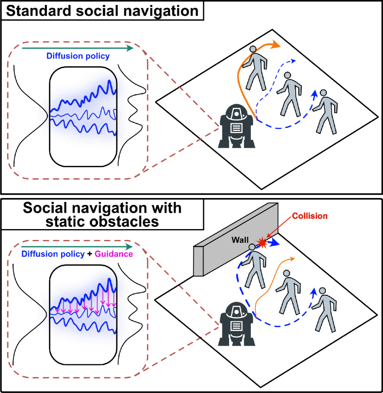
Figure 1: Conceptual diagram of the proposed method. In standard social navigation, the proposed method leverages the multimodality of diffusion models to generate various actions that allow the robot to avoid pedestrians. The blue dashed arrows represent examples of candidate actions generated for this situation, while the solid orange line indicates the actual action selected (upper window). In environments with static obstacles, actions generated solely by the diffusion model may result in collisions with walls. Therefore, guidance is applied to steer the selection toward alternative candidates that avoid wall collisions (lower window).

Social navigation, which enables safe and efficient navigation in dynamic environments with pedestrian traffic, is crucial for realizing autonomous mobile service robots. In recent years, driven by advancements in machine learning, deep reinforcement learning-based methods have been studied extensively. Among these, methods that assume a continuous action space require modeling of the action distribution using predefined functions, such as Gaussian distributions. Generative models, a branch of machine learning, have seen remarkable advancements, with diffusion models achieving significant success in fields such as image generation. Their application to reinforcement learning has also been explored, and they can reportedly achieve a high performance in continuous action spaces owing to their expressive capacity and lack of reliance on a Gaussian distribution assumption. However, diffusion models have not yet been applied to social navigation. Therefore, this study applied a diffusion-based reinforcement learning approach to mobile robot navigation in dynamic environments with pedestrian traffic.

In addition, many deep reinforcement learning-based methods face challenges adapting to conditions that are not considered during training. For instance, methods trained in environments with only pedestrians struggle when deployed in environments with static obstacles, such as walls. This study aimed to address this issue by utilizing guidance, a technique that allows the incorporation of post-training constraints during action generation using diffusion models without additional training. Considering these adaptability features, the proposed method is called Controllable L earning-based Social Navigation (COLSON). A conceptual diagram of COLSON is shown in Fig. 1.

The main contributions of this study are as follows:

• We integrate a diffusion-based reinforcement learning method with a graph neural network (GNN) architecture and apply it to social navigation.

• We demonstrate that the proposed method can handle conditions that are not considered during training, such as trajectory smoothing and adaptation to environments with static obstacles, without requiring additional training.

• Through comparative experiments with conventional methods, we show that the proposed method outperforms existing approaches and exhibits high performance, even in environments where the number of pedestrians differs from that in the training phase, highlighting its scalability.

• We conducted a real-world demonstration to validate that the proposed method can effectively control an actual robot in practical situations.

II RELATED WORK

II-A Social Navigation

Numerous deep reinforcement learning-based social navigation methods have been proposed. Chen et al. [1] introduced value-based learning models for multi-agent collision avoidance, marking a pioneering achievement in deep reinforcement learning approaches aimed at enabling autonomous mobile robots to safely navigate dynamic environments. Building on this, Chen et al. [2] proposed a method that incorporates social norms into the reward function to improve pedestrian collision avoidance and further addressed the challenge of pedestrian switching in multi-agent scenarios by sharing weights in the pedestrian information processing layer and employing max pooling. In addition to the direct application of deep reinforcement learning, architectural improvements in neural networks have been explored to enhance performance and develop methods that can accommodate an arbitrary number of agents [3, 4, 5, 6, 7, 8]. Other studies have expanded the scope beyond performance enhancement and scalability to pedestrian density by investigating approaches that leverage human gaze information [9], utilize map-based processing to enable navigation in environments with both static and dynamic obstacles [10, 11], and incorporate continuous action spaces [12]. More recently, hybrid approaches that integrate reinforcement learning-based methods with rule-based methods have been proposed to further enhance robustness and adaptability [13, 14].

II-B Diffusion Models for Action Generation

Diffusion models have achieved remarkable success in various data generation tasks, including image synthesis [15, 16, 17]. Recent studies have extended their applications beyond vision-based data to action generation in robotics through imitation learning and reinforcement learning. In the field of imitation learning, Janner et al. and Reuss et al. proposed methods based on behavior cloning (BC) [18, 19], where diffusion models were trained to generate actions that replicate target demonstration data, making it the most fundamental approach for applying diffusion models to action generation. In addition to imitation learning, diffusion models have been applied to offline reinforcement learning [20, 21, 22, 23], where exploration is not required, allowing models to learn distributions from datasets in a manner similar to that of imitation learning.

More recently, efforts have been directed toward applying diffusion models to online reinforcement learning [24], particularly in settings that differ from conventional diffusion model formulations, such as learning without access to pre-sampled data from an optimal target distribution [25] and approaches based on weighted regression [26].

Furthermore, in the context of applying diffusion models to mobile robots, methods leveraging diffusion policy for goal-conditioned navigation and undirected exploration have been proposed [27]. Other approaches use models trained on ground truth data from the A^⋆ algorithm for global path planning [28, 29].

III PRELIMINARIES

This study addresses the problem of two-dimensional (2D) mobile robot navigation while ensuring collision avoidance with pedestrians. The robot’s state includes its position from the goal, velocity, and orientation information: $\boldsymbol{s}^{r}=\left[{}^{g}\boldsymbol{p}^{r},\boldsymbol{v}^{r},\theta\right]$. By contrast, the position and velocity information of each pedestrian is converted to a robot-centered coordinate system and adopted as a state $\boldsymbol{s}^{n}=\left[{}^{rc}\boldsymbol{p}^{n},^{rc}\boldsymbol{v}^{n}\right]$. The set of pedestrian states in the environment is described by $\boldsymbol{s}^{h}=\left[\boldsymbol{s}^{1},\boldsymbol{s}^{2},\dots,\boldsymbol{s}^{n}\right]$. The robot obtains rewards after performing actions. $R_{t}$ denotes the reward function at time $t$ as follows:

$$R_{t}=\left\{\begin{array}[]{ll}-0.25&\text{ if }d_{t}<0\\ -0.1+d_{t}/2&\text{ else if }d_{t}<0.2\\ 1&\text{ else if }\boldsymbol{p}^{r}_{t}=\boldsymbol{p}^{g}_{t}\\ 0&\text{ otherwise }\end{array}\right.,$$ (5)

where $d_{t}$ is the minimum separation distance between the robot and pedestrians, $\boldsymbol{p}_{t}^{r}$ is the robot’s position, and $\boldsymbol{p}_{t}^{g}$ is the goal position at time $t$.

IV APPROACH

In this section, the model architecture, training methodology, and guidance methods for path smoothing and static obstacle avoidance are presented.

IV-A Model Architecture

The model architecture of the proposed method is illustrated in Fig. 2.

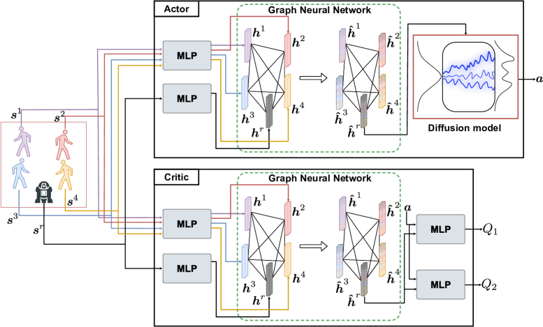
Figure 2: Architecture of proposed method. $\boldsymbol{s}^{r}$ and $\boldsymbol{s}^{n}$ indicate the states of each robot and pedestrian, respectively. $\boldsymbol{h}^{n}$ indicates the features of each robot and pedestrian. $\boldsymbol{\hat{h}}^{n}$ indicates the features after the GNN is applied.

This model adopts an Actor-Critic framework in which both the Actor and Critic incorporate GNNs. Each GNN utilizes Graph Attention Networks v2 (GATv2) [30]. The Actor employs a diffusion model that considers the output of the GNN as a condition and generates actions. The Critic network inputs the output of the GNN into a multi-layer perceptron to compute Q-values.

IV-B Q-Score Matching

In this study, we used Q-score matching (QSM) [25] as the training framework. Diffusion models are typically trained using score functions for the target distribution. However, in reinforcement learning, where the objective is to learn an optimal policy, the optimal policy is unknown. Consequently, neither the score function nor samples from the optimal policy can be precomputed. To overcome this challenge, QSM facilitates reinforcement learning with diffusion models by leveraging the action gradient of the Q-function as a score. The training procedure using QSM is presented in Algorithm 1.

1 Initialize score network $\Psi_{\theta}$ and critic networks $Q_{\phi^{1}}$ and $Q_{\phi^{2}}$

2 Set parameter values of the target critics $Q_{\phi^{\prime,1}}$ and $Q_{\phi^{\prime,2}}$ equal to those of the main critics

3 for $i=1$ to $E$ do

4    Explore using the policy until finishing an episode

5    After finishing an episode, store the trajectory of $\left(\boldsymbol{s}_{t},\boldsymbol{a}_{t},r_{t},\boldsymbol{s}^{\prime}_{t}\right)$ to the replay buffer $\mathcal{D}$

6    Sample a batch $\mathcal{B}=\{(\boldsymbol{s},\boldsymbol{a},r,\boldsymbol{s}^{\prime})$} from the replay buffer $\mathcal{D}$

7    Sample actions for computing targets $\quad\boldsymbol{\hat{a}}^{\prime}\sim\pi_{\theta}\left(\cdot\mid\boldsymbol{s}^{\prime}\right)$

8    Calculate targets for the Q-function $y\left(r,\boldsymbol{s}^{\prime}\right)=r+\gamma\left(\min_{i=1,2}Q_{\phi^{\prime,i}}\left(\boldsymbol{s}^{\prime},\boldsymbol{\hat{a}}^{\prime}\right)\right)$

9    Update critics by minimizing $L_{\text{critic}}=\displaystyle\frac{1}{|\mathcal{B}|}\sum(Q_{\phi^{i}}(\boldsymbol{s},\boldsymbol{a})-y\left(r,\boldsymbol{s}^{\prime}\right))^{2}$   for $i=1,2$

10    Update score network by minimizing $L_{\text{QSM}}=\displaystyle\frac{1}{|\mathcal{B}|}\sum\lVert\Psi_{\theta}(\boldsymbol{s},\boldsymbol{a})-\alpha\nabla_{a}Q(\boldsymbol{s},\boldsymbol{a})\rVert^{2}$

11    Update the target critic by polyak averaging $\phi^{\prime,i}\leftarrow\rho\phi^{\prime,i}+(1-\rho)\phi_{i}$   for $i=1,2$

12 end for

Algorithm 1 Training algorithm using QSM

The coefficient $\alpha$ required for computing the loss function must be set by considering the possible values of the Q-function and the scale of the final actions. In this study, several configurations of $\alpha$ were tested, and the best configuration was selected.

IV-C Guidance for Smooth Action Generation

As an initial demonstration of the proposed method’s extensibility, we show that action smoothing can be achieved during generation without additional training by introducing additional constraints. The reward function in this study prioritizes reaching the goal and avoiding collisions but does not account for trajectory smoothness. Consequently, the generated actions often exhibit abrupt movements. To address this issue, we employ Stochastic Differential Editing (SDEdit) [31] for smoothing. Diffusion models generate outputs by progressively removing Gaussian noise. SDEdit modifies this process by initializing it with reference data augmented with noise, guiding the generated data to approximate the desired output. In our method, the actions from the previous step serve as the guide data. The execution procedure for smoothing with SDEdit is presented in Algorithm 2.

IV-D Guidance for Static Obstacle Avoidance

As a second demonstration of the proposed method’s extensibility, we show that guidance enables the robot to navigate around static obstacles that were absent during training without further training.

Input: Trained score network $\Psi_{\theta}$, states $\boldsymbol{s}_{t}=\left[\boldsymbol{s}_{t}^{r},\boldsymbol{s}_{t}^{h}\right]$ at time $t$ Previous action $\boldsymbol{a}_{t-1}$, hyperparameter $T$, $\alpha_{\tau}$

1 $\boldsymbol{z}=\mathcal{N}(\bm{0},\bm{I})$

2 $\boldsymbol{x}_{0}=\boldsymbol{a}_{t-1}$

3 for $\tau=1$ to $T$ do

4    $\boldsymbol{x}_{\tau}=\sqrt{1-\alpha_{\tau}}\boldsymbol{x}_{\tau-1}+\sqrt{\alpha_{\tau}}\boldsymbol{z}$

5   

6 end for

7for $\tau=T$ to $1$ do

8    Denoise by score employing $\boldsymbol{x}_{\tau-1}=\frac{1}{\sqrt{1-\alpha_{\tau}}}\boldsymbol{x}_{\tau}-\frac{\sqrt{\alpha}_{\tau}}{\sqrt{1-\alpha_{\tau}}}\Psi_{\theta}(\boldsymbol{s_{t}},\boldsymbol{x}_{\tau},\tau)$

9   

10 end for

11Execute the action $\boldsymbol{a}_{t}=\boldsymbol{x}_{0}$

Algorithm 2 Action generation with guidance for smoothing

The training environment in this study contained only pedestrians, implying that the learned policy lacks the capability to avoid static obstacles.

TABLE I: Numerical comparison in circle-crossing scenario with 5 ORCA pedestrians

	Visible				Invisible
Method	Success [%] $\uparrow$	Collision [%] $\downarrow$	Exec. time [s] $\downarrow$	Return $\uparrow$		Success [%] $\uparrow$	Collision [%] $\downarrow$	Exec. time [s] $\downarrow$	Return $\uparrow$
ORCA (for reference)	$100.00\pm 0.00$	$0.00\pm 0.00$	$10.02\pm 0.00$	$0.542\pm 0.000$		$42.80\pm 0.00$	$56.80\pm 0.00$	$10.93\pm 0.00$	$0.081\pm 0.000$
BC	$77.28\pm 0.17$	$22.56\pm 0.18$	$10.06\pm 0.61$	$0.377\pm 0.001$		$5.08\pm 0.21$	$94.92\pm 0.21$	$10.24\pm 0.81$	$-0.182\pm 0.002$
AWR	$87.60\pm 1.96$	$12.36\pm 1.97$	$11.44\pm 1.80$	$0.466\pm 0.009$		$42.44\pm 4.78$	$57.56\pm 4.78$	$11.48\pm 2.16$	$0.122\pm 0.030$
CAWR	$61.00\pm 0.57$	$35.28\pm 0.45$	$11.98\pm 8.13$	$0.236\pm 0.001$		$12.48\pm 2.11$	$86.68\pm 2.34$	$12.96\pm 10.21$	$0.122\pm 0.030$
QVWR	$62.48\pm 3.84$	$34.24\pm 3.86$	$11.44\pm 5.63$	$0.245\pm 0.020$		$6.68\pm 1.00$	$92.92\pm 1.10$	$11.44\pm 6.04$	$-0.173\pm 0.007$
AWAC	$71.08\pm 2.91$	$28.92\pm 2.91$	$11.32\pm 5.83$	$0.327\pm 0.011$		$29.76\pm 7.20$	$70.24\pm 7.20$	$11.31\pm 5.69$	$0.010\pm 0.038$
DIPO	$80.80\pm 1.97$	$17.52\pm 1.42$	$11.29\pm 1.26$	$0.327\pm 0.011$		$30.32\pm 3.41$	$68.96\pm 3.03$	$12.22\pm 0.15$	$0.022\pm 0.021$
QVPO	$98.24\pm 0.02$	$1.68\pm 0.01$	$9.75\pm 0.97$	$0.618\pm 0.001$		$97.44\pm 0.03$	$2.36\pm 0.03$	$9.99\pm 0.79$	$0.606\pm 0.001$
COLSON (QSM)	$\mathbf{98.28}\pm\mathbf{0.03}$	$\mathbf{1.60}\pm\mathbf{0.03}$	$\mathbf{8.70}\pm\mathbf{0.07}$	$\mathbf{0.647}\pm\mathbf{0.000}$		$\mathbf{98.44}\pm\mathbf{0.01}$	$\mathbf{1.32}\pm\mathbf{0.01}$	$\mathbf{9.05}\pm\mathbf{0.05}$	$\mathbf{0.640}\pm\mathbf{0.000}$

TABLE II: Numerical comparison in circle-crossing scenario with 5 social force pedestrians

	Visible				Invisible
Method	Success [%] $\uparrow$	Collision [%] $\downarrow$	Exec. time [s] $\downarrow$	Return $\uparrow$		Success [%] $\uparrow$	Collision [%] $\downarrow$	Exec. time [s] $\downarrow$	Return $\uparrow$
ORCA (for reference)	$90.80\pm 0.00$	$9.20\pm 0.00$	$9.79\pm 0.00$	$0.544\pm 0.000$		$19.00\pm 0.00$	$81.00\pm 0.00$	$10.82\pm 0.00$	$-0.088\pm 0.000$
BC	$63.4\pm 1.30$	$36.6\pm 1.30$	$10.16\pm 0.73$	$0.303\pm 0.007$		$0.28\pm 0.00$	$99.72\pm 0.00$	$14.62\pm 75.05$	$-0.222\pm 0.000$
AWR	$86.92\pm 0.57$	$13.04\pm 0.58$	$11.52\pm 2.18$	$0.483\pm 0.007$		$41.68\pm 11.13$	$58.28\pm 11.16$	$11.37\pm 2.00$	$0.131\pm 0.076$
CAWR	$63.32\pm 1.94$	$34.20\pm 2.25$	$12.28\pm 11.09$	$0.278\pm 0.005$		$6.80\pm 0.90$	$92.48\pm 1.12$	$21.17\pm 70.54$	$-0.172\pm 0.006$
QVWR	$58.04\pm 0.89$	$36.36\pm 1.91$	$12.46\pm 7.28$	$0.245\pm 0.003$		$3.60\pm 0.33$	$96.08\pm 0.38$	$23.85\pm 70.94$	$-0.196\pm 0.003$
AWAC	$80.64\pm 3.24$	$19.32\pm 3.25$	$11.47\pm 7.14$	$0.431\pm 0.022$		$42.68\pm 6.67$	$57.32\pm 6.67$	$15.53\pm 70.50$	$0.127\pm 0.048$
DIPO	$73.52\pm 0.41$	$25.00\pm 0.24$	$12.06\pm 1.30$	$0.362\pm 0.001$		$6.88\pm 0.63$	$92.32\pm 0.54$	$12.80\pm 0.72$	$-0.154\pm 0.004$
QVPO	$\mathbf{99.88}\pm\mathbf{0.00}$	$\mathbf{0.04}\pm\mathbf{0.00}$	$9.47\pm 1.08$	$0.642\pm 0.001$		$96.72\pm 0.08$	$3.20\pm 0.08$	$9.76\pm 0.99$	$0.607\pm 0.002$
COLSON (QSM)	$99.60\pm 0.00$	$0.40\pm 0.00$	$\mathbf{8.40}\pm\mathbf{0.03}$	$\mathbf{0.669}\pm\mathbf{0.000}$		$\mathbf{98.72}\pm\mathbf{0.00}$	$\mathbf{1.20}\pm\mathbf{0.00}$	$\mathbf{8.62}\pm\mathbf{0.07}$	$\mathbf{0.654}\pm\mathbf{0.000}$

Input: Trained score network $\Psi_{\theta}$, states $\boldsymbol{s}_{t}=\left[\boldsymbol{s}_{t}^{r},\boldsymbol{s}_{t}^{h}\right]$ at time $t$, previous action $\boldsymbol{a}_{t-1}$, current robot position $\boldsymbol{p}^{r}$, safety distance $d_{s}$, hyperparameter $\eta$, $T$, $\alpha_{\tau}$, distance cost $c_{d}$, lethal cost $c_{l}$

1 $\boldsymbol{x}_{T}=\mathcal{N}(\bm{0},\bm{I})$

2

3for $\tau=T$ to $1$ do

4    Calculate next robot position $\hat{\boldsymbol{p}}^{r}=\boldsymbol{p}^{r}+\boldsymbol{x}_{\tau}\Delta t$ and difference from the nearest point of static obstacles $\boldsymbol{d}$

5    Calculate vector for guidance to avoid static obstacles

6    $\boldsymbol{g}_{o}=\begin{cases}\frac{\boldsymbol{d}}{|\boldsymbol{d}|}c_{l}&\text{ if }\hat{\boldsymbol{p}}^{r}\text{is inside of obstacles}\\ \frac{\boldsymbol{d}}{|\boldsymbol{d}|}c_{d}&\text{ else if }0<|\boldsymbol{d}|\leq d_{s}\\ \frac{\boldsymbol{d}}{|\boldsymbol{d}|}c_{d}\exp(\eta(d_{s}-|\boldsymbol{d}|))&\text{otherwise}\end{cases}$

7    Denoise by score and guidance employing $\boldsymbol{x}_{\tau-1}=\frac{1}{\sqrt{1-\alpha_{\tau}}}\boldsymbol{x}_{\tau}-\frac{\sqrt{\alpha}_{\tau}}{\sqrt{1-\alpha_{\tau}}}\Psi_{\theta}(\boldsymbol{s_{t}},\boldsymbol{x}_{\tau},\tau)$ + $\boldsymbol{g}_{o}$

8   

9 end for

10Execute the action $\boldsymbol{a}_{t}=\boldsymbol{x}_{0}$

Algorithm 3 Action generation with guidance for static obstacle avoidance

To address this, we incorporate guidance into the diffusion model to steer actions away from static obstacles, allowing the robot to avoid both pedestrians and static obstacles. In particular, the guidance strength increases as the robot approaches a wall, directing its movement away from the obstacle. The execution procedure for this guidance is presented in Algorithm 3.

V EXPERIMENTS

Experiments were conducted in a simulation environment to evaluate the effectiveness of the proposed method.

V-A Simulation Environment and Settings

We employed the CrowdNav environment adopted in some related studies [4, 5]. In this environment, pedestrians are controlled by ORCA [32]. The models were trained for 100,000 episodes in a visible circle crossing scenario with 5 pedestrians. Additionally, data were collected using ORCA before each training session, and training began with a dataset of 2000 episodes. The hyperparameter $\alpha$ of QSM was set to 400. The number of generation steps was set to 100 for each diffusion-based reinforcement learning method.

V-B Performance Evaluation

The performance of each method was evaluated in a circle crossing scenario with pedestrians controlled by ORCA and another scenario with pedestrians controlled by the social force model. In each scenario, the methods was evaluated under two conditions: one where pedestrians were aware of the robot’s position (visible) and another where they were unaware (invisible). For comparison, the proposed method was evaluated against BC, CAWR [12], which tackles social navigation with continuous action spaces, and related reinforcement learning methods, such as AWR [33], QVWR [34], and AWAC [35]. Furthermore, comparisons were made with diffusion model-based reinforcement learning methods, including DIPO [24] and QVPO [26]. For each method, five models were trained with different random seeds. The evaluation metrics included success rate, collision rate, average execution time, and average return. The test scenarios comprised 500 episodes each.

The results are summarized in Tables I and II. The $\pm$ symbol in each table indicates the standard deviation computed from the results of training runs using five independent random seeds. In scenarios where pedestrians were controlled using ORCA, the proposed method achieved the best performance under both the visible and invisible conditions. In scenarios where pedestrians were controlled using the social force model, QVPO achieved better results in terms of success and collision rates under the visible condition. However, the proposed method executed approximately 1 s faster and achieved higher returns. In the invisible setting, the proposed method outperformed all categories.

Fig. 3 shows a comparison of success rates as the number of pedestrians increases in the circle crossing scenario. The proposed method consistently outperformed the other approaches across all pedestrian densities. The performance gap with QVPO is small for five pedestrians but widens as the population increases. This trend is likely due to QVPO’s reliance on weighted regression, which limits generalization to unseen scenarios.

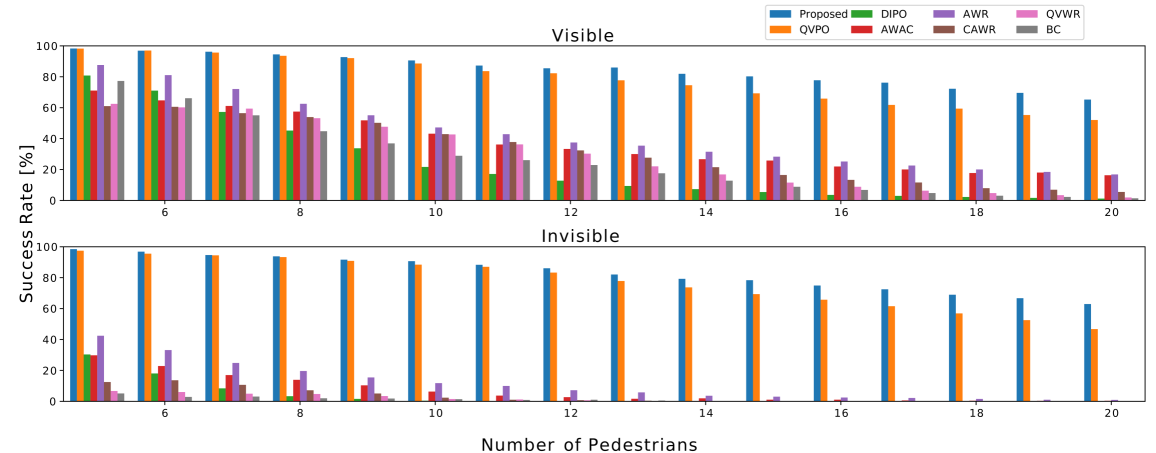
Figure 3: Comparison of success rate while changing the number of pedestrians. The upper graph shows the results for the visible setting, while the lower graph presents the results for the invisible setting.

V-C Evaluation of Smoothing

The effectiveness of smoothing through guidance using SDEdit was evaluated in the circle crossing scenario with 20 pedestrians, where action oscillations were prominent. Fig. 4 presents a qualitative comparison, showing that trajectories generated with SDEdit-based smoothing are noticeably smoother. In addition, Table III provides a quantitative comparison of success rate and trajectory smoothness. Trajectory smoothness was evaluated using a measure from a previous study [36]. The numerical evaluation results indicate that although SDEdit reduces the success rate, it significantly enhances trajectory smoothness. Despite a slight decrease in success rate, reduced execution time results in a higher return. This is likely because improved smoothness allows surrounding pedestrians to avoid the robot more easily.

TABLE III: Numerical comparison for smoothing

Method	Success [%]$\uparrow$	Collision [%]$\downarrow$	Exec. time [s]$\downarrow$	Return $\uparrow$	Smoothness$\cdot 10^{3}$ $\downarrow$
w/o guidance	$\mathbf{82.60}$	$\mathbf{17.20}$	$11.35$	$0.445$	$43.09$
w guidance	$82.00$	$17.40$	$\mathbf{10.97}$	$\mathbf{0.448}$	$\mathbf{9.16}$

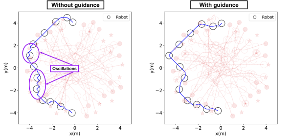
Figure 4: Trajectory of robot with and without guidance for smoothing. The blue lines represent the trajectory of the robot’s movement, while the light red lines indicate the trajectories of pedestrian movements.

V-D Evaluation of Static Obstacle Avoidance

The effectiveness of the guidance for static obstacle avoidance was evaluated in an environment with walls and three pedestrians approaching from the front. Fig. 5 presents a qualitative comparison. The results show that when the robot initially intended to move left to avoid pedestrians, leading to a potential collision with the wall, shifting to the right by the guidance instead allowed it to evade both pedestrians and the wall. Table IV presents a quantitative comparison of cases with and without guidance. In the table, Col-P represents the collision rate with pedestrians, and Col-W represents the collision rate with walls. The results show that the proposed guidance method significantly reduces collisions with walls and greatly improves the success rate.

TABLE IV: Numerical comparison in environments with static obstacles

Method	Success [%]$\uparrow$	Col-P [%]$\downarrow$	Col-W [%]$\downarrow$	Exec. time [s]$\downarrow$	Return$\uparrow$
w/o guidance	$52.8$	$\mathbf{0.04}$	$46.8$	$8.00$	$0.261$
w guidance	$\mathbf{95.6}$	$0.08$	$\mathbf{3.6}$	$\mathbf{7.99}$	$\mathbf{0.645}$

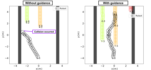
Figure 5: Comparison between with and without guidance for static obstacle avoidance. Colored circles represent pedestrian trajectories, and the black rectangles represent walls.

VI Real-World Demonstration

A real-world demonstration was conducted using the developed robot system. The system is based on a Mecanum rover and is equipped with a 2D-LiDAR (UST-20LX) and onboard computer (Jetson AGX Orin) for processing. The software system was built using ROS2 Humble, and pedestrian detection was performed using DR-SPAAM [37, 38]. Additionally, localization was realized using adaptive Monte Carlo localization (AMCL).

\begin{overpic}[width=213.39566pt]{figs/real_world_experiment_3.pdf} \put(1.0,51.0){\Circled[fill color=white]{1}} \put(51.0,51.0){\Circled[fill color=white]{2}} \put(1.0,22.0){\Circled[fill color=white]{3}} \put(51.0,22.0){\Circled[fill color=white]{4}} \end{overpic}

Figure 6: Scenes of the real-world demonstration using the proposed method.

The demonstration setup is shown in Fig. 6. The results confirm that the proposed method is capable of controlling a real robot.

Meanwhile, the average action generation time for the proposed method was 0.28 s, with a maximum of 0.41 s with the robot system. Given that the training environment used a 0.25 s time interval, further speed optimization is necessary. Future studies should address this issue.

VII CONCLUSIONS

In this study, we applied diffusion-based reinforcement learning trained with QSM for social navigation and demonstrated that it outperforms other methods. In addition, we demonstrated that by utilizing guidance, conditions that were not considered during training could be incorporated without additional training. In future, we plan to extend the applicability of the proposed method to a wider range of scenarios and conduct more detailed real-world experiments to further enhance its performance.

References

- [1] Y. F. Chen, M. Liu, M. Everett, and J. P. How, “Decentralized Non-communicating Multiagent Collision Avoidance with Deep Reinforcement Learning,” in Proceedings of the IEEE International Conference on Robotics and Automation (ICRA), pp. 285–292, 2017.
- [2] Y. F. Chen, M. Everett, M. Liu, and J. P. How, “Socially Aware Motion Planning with Deep Reinforcement Learning,” in Proceedings of the IEEE/RSJ International Conference on Intelligent Robots and Systems (IROS), pp. 1343–1350, 2017.
- [3] M. Everett, Y. F. Chen, and J. P. How, “Motion Planning among Dynamic, Decision-Making Agents with Deep Reinforcement Learning,” in Proceedings of the IEEE/RSJ International Conference on Intelligent Robots and Systems (IROS), pp. 3052–3059, 2018.
- [4] C. Chen, Y. Liu, S. Kreiss, and A. Alahi, “Crowd-Robot Interaction: Crowd-aware Robot Navigation with Attention-based Deep Reinforcement Learning,” in Proceedings of the IEEE International Conference on Robotics and Automation (ICRA), pp. 6015–6022, 2019.
- [5] C. Chen, S. Hu, P. Nikdel, G. Mori, and M. Savva, “Relational Graph Learning for Crowd Navigation,” in Proceedings of the IEEE/RSJ International Conference on Intelligent Robots and Systems (IROS), pp. 10007–10013, 2020.
- [6] K. Matsumoto, A. Kawamura, Q. An, and R. Kurazume, “Mobile Robot Navigation Using Learning-Based Method Based on Predictive State Representation in a Dynamic Environment,” in Proceedings of the IEEE/SICE International Symposium on System Integration (SII), pp. 499–504, 2022.
- [7] Y. Yang, J. Jiang, J. Zhang, J. Huang, and M. Gao, “ST2: Spatial-Temporal state transformer for Crowd-Aware autonomous navigation,” IEEE Robotics and Automation Letters, vol. 8, no. 2, pp. 912–919, 2023.
- [8] S. Liu, P. Chang, Z. Huang, N. Chakraborty, K. Hong, W. Liang, D. Livingston McPherson, J. Geng, and K. Driggs-Campbell, “Intention Aware Robot Crowd Navigation with Attention-Based Interaction Graph,” in Proceedings of the IEEE International Conference on Robotics and Automation (ICRA), pp. 12015–12021, 2023.
- [9] Y. Chen, C. Liu, B. E. Shi, and M. Liu, “Robot Navigation in Crowds by Graph Convolutional Networks With Attention Learned From Human Gaze,” IEEE Robotics and Automation Letters, vol. 5, no. 2, pp. 2754–2761, 2020.
- [10] L. Lucia, D. Daniel, C. Gianluca, S. Roland, and D. Renaud, “Robot Navigation in Crowded Environments Using Deep Reinforcement Learning,” in Proceedings of the IEEE/RSJ International Conference on Intelligent Robots and Systems (IROS), pp. 5671–5677, 2020.
- [11] S. Yao, G. Chen, Q. Qiu, J. Ma, X. Chen, and J. Ji, “Crowd-Aware Robot Navigation for Pedestrians with Multiple Collision Avoidance Strategies via Map-based Deep Reinforcement Learning,” in Proceedings of the IEEE/RSJ International Conference on Intelligent Robots and Systems (IROS), pp. 8144–8150, 2021.
- [12] X. Zhang, W. Xi, X. Guo, Y. Fang, B. Wang, W. Liu, and J. Hao, “Relational Navigation Learning in Continuous Action Space among Crowds,” in Proceedings of the IEEE International Conference on Robotics and Automation (ICRA), pp. 3175–3181, 2021.
- [13] J. Wu, Y. Wang, H. Asama, Q. An, and A. Yamashita, “Risk-Sensitive Mobile Robot Navigation in Crowded Environment via Offline Reinforcement Learning,” in Proceedings of the IEEE/RSJ International Conference on Intelligent Robots and Systems (IROS), pp. 7456–7462, 2023.
- [14] K. Matsumoto, Y. Hyodo, and R. Kurazume, “Crowd-Aware Robot Navigation with Switching Between Learning-Based and Rule-Based Methods Using Normalizing Flows,” in Proceedings of the IEEE/RSJ International Conference on Intelligent Robots and Systems (IROS), pp. 4823–4830, 2024.
- [15] J. Ho, A. Jain, and P. Abbeel, “Denoising Diffusion Probabilistic Models,” in Advances in Neural Information Processing Systems (NeurIPS), pp. 6840–6851, 2020.
- [16] R. Rombach, A. Blattmann, D. Lorenz, P. Esser, and B. Ommer, “High-Resolution Image Synthesis with Latent Diffusion Models,” in Proceedings of the IEEE/CVF Conference on Computer Vision and Pattern Recognition (CVPR), pp. 10674–10685, 2022.
- [17] K. Nakashima and R. Kurazume, “LiDAR Data Synthesis with Denoising Diffusion Probabilistic Models,” in Proceedings of the IEEE International Conference on Robotics and Automation (ICRA), pp. 14724–14731, 2024.
- [18] M. Janner, Y. Du, J. B. Tenenbaum, and S. Levine, “Planning with Diffusion for Flexible Behavior Synthesis,” in Proceedings of the International Conference on Machine Learning (ICML), pp. 9902–9915, 2022.
- [19] M. Reuss, M. Li, X. Jia, and R. Lioutikov, “Goal-Conditioned Imitation Learning using score-based Diffusion Policies,” in Proceedings of the Robotics: Science and Systems (RSS), 2023.
- [20] Z. Wang, J. J. Hunt, and M. Zhou, “Diffusion Policies as an Expressive Policy Class for Offline Reinforcement Learning,” in Proceedings of the International Conference on Learning Representations (ICLR), 2023.
- [21] H. J. Terry Suh, G. Chou, H. Dai, L. Yang, A. Gupta, and R. Tedrake, “Fighting Uncertainty with Gradients: Offline Reinforcement Learning via Diffusion Score Matching,” in Proceedings of the Annual Conference on Robot Learning (CoRL), pp. 2878–2904, 2023.
- [22] B. Kang, X. Ma, C. Du, T. Pang, and Y. A. N. Shuicheng, “Efficient Diffusion Policies For Offline Reinforcement Learning,” in Advances in Neural Information Processing Systems (NeurIPS), pp. 67195–67212, 2023.
- [23] P. Hansen-Estruch, I. Kostrikov, M. Janner, J. G. Kuba, and S. Levine, “IDQL: Implicit Q-Learning as an Actor-Critic Method with Diffusion Policies,” CoRR, vol. abs/2304.10573, 2023.
- [24] L. Yang, Z. Huang, F. Lei, Y. Zhong, Y. Yang, C. Fang, S. Wen, B. Zhou, and Z. Lin, “Policy Representation via Diffusion Probability Model for Reinforcement Learning,” CoRR, vol. abs/2305.13122, 2023.
- [25] M. Psenka, A. Escontrela, P. Abbeel, and Y. Ma, “Learning a Diffusion Model Policy from Rewards via Q-Score Matching,” in Proceedings of the International Conference on Machine Learnin (ICML), pp. 41163–41182, 2024.
- [26] S. Ding, K. Hu, Z. Zhang, K. Ren, W. Zhang, J. Yu, J. Wang, and Y. Shi, “Diffusion-based Reinforcement Learning via Q-weighted Variational Policy Optimization,” in Advances in Neural Information Processing Systems (NeurIPS), pp. 53945–53968, 2024.
- [27] A. Sridhar, D. Shah, C. Glossop, and S. Levine, “NoMaD: Goal Masked Diffusion Policies for Navigation and Exploration,” in Proceedings of the IEEE International Conference on Robotics and Automation (ICRA), pp. 63–70, 2024.
- [28] J. Liu, M. Stamatopoulou, and D. Kanoulas, “DiPPeR: Diffusion-based 2D Path Planner applied on Legged Robots,” in Proceedings of the IEEE International Conference on Robotics and Automation (ICRA), pp. 9264–9270, 2024.
- [29] M. Stamatopoulou, J. Liu, and D. Kanoulas, “DiPPeST: Diffusion-based path planner for synthesizing trajectories applied on quadruped robots,” in Proceedings of the IEEE/RSJ International Conference on Intelligent Robots and Systems (IROS), pp. 7787–7793, 2024.
- [30] S. Brody, U. Alon, and E. Yahav, “How Attentive are Graph Attention Networks?,” in Proceedings of the International Conference on Learning Representations (ICLR), 2022.
- [31] C. Meng, Y. He, Y. Song, J. Song, J. Wu, J.-Y. Zhu, and S. Ermon, “SDEdit: Guided Image Synthesis and Editing with Stochastic Differential Equations,” in Proceedings of the International Conference on Learning Representations (ICLR), 2022.
- [32] J. Van Den Berg, S. J. Guy, M. Lin, and D. Manocha, “Reciprocal n-Body Collision Avoidance,” in Proceedings of the International Symposium of Robotic Research, pp. 3–19, 2011.
- [33] X. B. Peng, A. Kumar, G. Zhang, and S. Levine, “Advantage-Weighted Regression: Simple and Scalable Off-Policy Reinforcement Learning,” CoRR, vol. abs/1910.00177, 2019.
- [34] P. Kozakowski, L. Kaiser, H. Michalewski, A. Mohiuddin, and K. Kańska, “Q-Value Weighted Regression: Reinforcement Learning with Limited Data,” in Proceedings of the International Joint Conference on Neural Networks (IJCNN), pp. 1–8, 2022.
- [35] A. Nair, M. Dalal, A. Gupta, and S. Levine, “AWAC: Accelerating Online Reinforcement Learning with Offline Datasets,” CoRR, vol. abs/2006.09359, 2020.
- [36] S. Mysore, B. Mabsout, R. Mancuso, and K. Saenko, “Regularizing Action Policies for Smooth Control with Reinforcement Learning,” in Proceedings of the IEEE International Conference on Robotics and Automation (ICRA), pp. 1810–1816, 2021.
- [37] D. Jia, A. Hermans, and B. Leibe, “DR-SPAAM: A Spatial-Attention and Auto-regressive Model for Person Detection in 2D Range Data,” in Proceedings of the IEEE/RSJ International Conference on Intelligent Robots and Systems (IROS), pp. 10270–10277, 2020.
- [38] D. Jia, M. Steinweg, A. Hermans, and B. Leibe, “Self-Supervised Person Detection in 2D Range Data using a Calibrated Camera,” in Proceedings of the IEEE International Conference on Robotics and Automation (ICRA), pp. 13301–13307, 2021.