Mixed spin-boson coupling for qubit readout
with suppressed residual shot-noise dephasing

Abstract

Direct dipole coupling between a two-level system and a bosonic mode describes the interactions present in a wide range of physical platforms. In this work, we study a coupling that is mixed between two pairs of quadratures of a bosonic mode and a spin. In this setting, we can suppress the dispersive shift while retaining a nonzero Kerr shift, which remarkably results in a cubic relationship between shot noise dephasing and thermal photons in the oscillator. We demonstrate this configuration with a simple toy model, quantify the expected improvements to photon shot-noise dephasing of the spin, and describe an approach to fast qubit readout via the Kerr shift. Further, we show how such a regime is achievable in superconducting circuits because magnetic and electric couplings can be of comparable strength, using two examples: the Cooper pair transistor and the fluxonium molecule.

I Introduction

Within the field of quantum technologies, it is imperative that we build qubit systems that allow for convenient methods to manipulate and readout the qubits [1, 2, 3, 4]. In many cases, these controls are achieved by coupling the qubit system coherently with bosonic modes [5, 6, 7]. For readout in particular, qubits are often coupled to a readout mode via a dipole-like coupling $\sigma_{i}(a^{\dagger}\pm a)$, where $i\in x,y$. The dipole coupling can manifest as a coupling of the quadratures $X=a^{\dagger}+a$ or $P=i(a^{\dagger}-a)$ to either the qubit operator $\sigma_{x}$ or to the operator $\sigma_{y}$ depending on its physical implementation. For example, superconducting qubits may be capacitively or inductively coupled to a readout resonator [8, 9, 10, 11, 12]. In these platforms, readout is commonly performed in the dispersive regime, where the resonator frequency shifts depending on the qubit state [13, 14]. Within perturbation theory, this response manifests in the Hamiltonian as $\chi\sigma_{z}a^{\dagger}a$. Thereby, the nature of the coupling (i.e., as arising from coupling either $X$ or $P$ of the resonator to either $\sigma_{x}$ or $\sigma_{y}$ of the qubit, or combinations thereof) is hidden.

The dispersive frequency shift also limits qubit performance. The qubit reciprocally picks up a frequency shift proportional to the number of photons in the resonator, also known as the ac-Stark shift [15]. This means that the residual average photon number $\bar{n}_{th}$ in the resonator will induce random shifts in the qubit frequency, leading to qubit dephasing rates that are linearly proportional to $\bar{n}_{th}$ [16, 17, 18, 19]. This dephasing channel is referred to as photon shot noise. For superconducting qubits, including transmon qubits and fluxonium qubits, which have intrinsic protection against charge dispersion and are linearly-protected to flux noise at sweetspots, photon shot noise is a limiting factor in coherence times [20, 21]. For example, to demonstrate large coherence times for fluxonium qubits, the dispersive shift $\chi$ is often designed to be much smaller than the readout resonator linewidth in order to protect the qubit from photon shot noise [22]. This has the effect of requiring longer readout times to achieve desired measurement fidelities. Previous works with superconducting qubits have also studied how adding extra nonlinear elements can circumvent some of the downsides of conventional dispersive readout such as reducing measurement-induced state-transition or Purcell decay [23, 24, 25, 9, 26]. However, these methods still rely on an effective dispersive Hamiltonian term that is intrinsically sensitive to photon shot-noise.

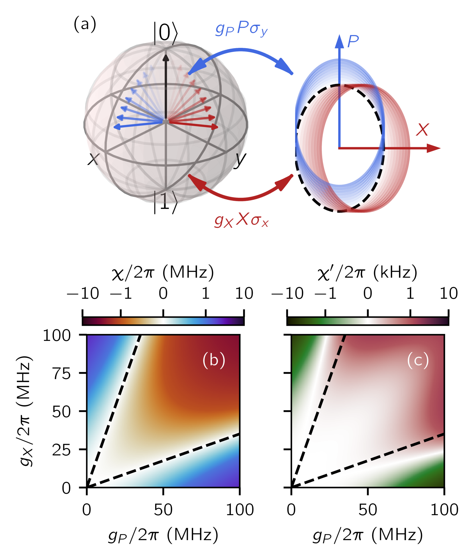
Figure 1: (a) Depiction of the mixed-coupling model. The Bloch sphere on the left shows the time evolution of the $\ket{0}$ state under the presence of the two couplings $g_{X}$ (red) and $g_{P}$ (blue). On the right, we show the corresponding phase space displacement of the harmonic oscillator for each coupling term. Symlog colormaps of dispersive (b) and Kerr (c) shifts as a function of the couplings $g_{X}$ and $g_{P}$. Here, we use $\omega_{q}/(2\pi)=$5\text{\,}\mathrm{GHz}$$ and $\omega_{r}/(2\pi)=$8\text{\,}\mathrm{GHz}$$ so that $|\omega_{q}-\omega_{r}|\gg g_{X},g_{P}$. The dashed lines indicate the analytical $\chi=0$ condition from Eq. (3). We show the $\chi=0$ condition also in panel (c) to indicate that these two corrections are not simultaneously suppressed.

In this work, we explore the scenario in which a qubit is coupled to a resonator mode through a mixed coupling, which in superconducting circuits can be achieved using a combination of inductive and capacitive elements [27, 28, 24]. Specifically, we pair $\sigma_{x}$ and $\sigma_{y}$ with distinct quadratures of a bosonic mode, see also Fig. 1, and demonstrate that a mixed coupling can provide a suppression of the dispersive shift. Remarkably, we find that the photon shot noise rate scales as the cube of the residual photon number $\bar{n}_{th}^{3}$ in this regime, implying significant improvements relative to usual dispersive coupling for typical $\bar{n}_{th}\sim 0.01$. Inspired by this result, we propose a nonlinear readout scheme by measuring through the next available term in perturbation theory, the Kerr shift $\chi^{\prime}\sigma_{z}a^{\dagger}a^{\dagger}aa$, and that this readout is competitive in both speed and fidelity. We show how to achieve mixed coupling in superconducting qubit circuits, making them ideal platforms for non-linear readout. By presenting a method that suppresses residual shot noise without the need for extra parametric drives, our work adds new features to readout that may support superconducting quantum circuits with increased performance.

II Mixed coupling and nonlinear readout

We first consider a minimal model, which consists of a qubit coupled to a resonator with the Hamiltonian

$$H=\hbar\frac{\omega_{q}}{2}\sigma_{z}+\hbar\omega_{r}a^{\dagger}a+H_{\text{coupling}}~,$$ (1)

where $\sigma_{i}$ are Pauli matrices acting in the qubit degrees of freedom, and $a^{\dagger}$ are creation and $a$ are annihilarion operators of the bosonic field, $\omega_{q}$ is the energy separation between the qubit levels, and $\omega_{r}$ is the frequency of the resonator. We consider a mixed coupling between the qubit and the resonator with Hamiltonian

$$H_{\text{coupling}}=\hbar g_{X}\sigma_{x}X+\hbar g_{P}\sigma_{y}P~,$$ (2)

with $X=a^{\dagger}+a$ and $P=i(a^{\dagger}-a)$. We remark that a realization of such a coupling where $g_{X}$ and $g_{P}$ are independently tunable allows obtaining a lab-frame Jaynes-Cummings Hamiltonian when $g_{X}=g_{P}$, while an anti-Jaynes-Cummings Hamiltonian is achieved with $g_{X}=-g_{P}$.

In the weak-coupling regime, $|g_{X}|,|g_{P}|\ll|\omega_{r}-\omega_{q}|$, we perform a Schrieffer-Wolff transformation that keeps non-rotating wave approximation (non-RWA) effects (see Appendix A). We then find that, within leading order in perturbation theory, the dispersive shift is

$$\chi=\frac{1}{\omega_{r}^{2}-\omega_{q}^{2}}\left[\omega_{q}(g_{X}^{2}+g_{P}^{2})-2\omega_{r}g_{P}g_{X}\right]~.$$ (3)

This expression is not monotonic in $g_{X}$ and $g_{P}$, thus, we see that it is possible to completely suppress the dispersive shift for non-zero $g_{X}$ and $g_{P}$, as shown in Fig. 1 (b). Moreover, we also see from the Schrieffer-Wolff transformation that we get non-linear corrections to the Hamiltonian in the form of

$$H_{Kerr}=\hbar\chi^{\prime}\sigma_{z}\,a^{\dagger}a^{\dagger}aa,$$ (4)

where we denote $\chi^{\prime}$ as the Kerr shift, i.e., a qubit-state-dependent Kerr coefficient, see Fig. 1 (c).

The nonlinear interaction term $\chi^{\prime}\sigma_{z}a^{\dagger}a^{\dagger}aa$ encodes the information about the qubit state in the change of resonator anharmonicity. More specifically, the Kerr shift $\chi^{\prime}$ can be written as

$$\chi^{\prime}=(K_{r,\ket{1}}-K_{r,\ket{0}})/4,$$ (5)

where $K_{r,\ket{q}}$ denotes the resonator anharmonicity when the qubit is $\ket{q}$ state. In this section, we demonstrate how we can use the Kerr shift to obtain efficient readout without suffering from residual shot noise.

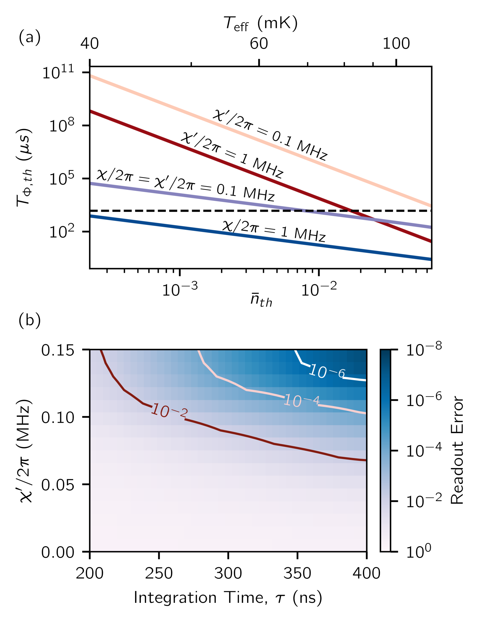
Figure 2: Nonlinear readout. (a) Qubit dephasing time limit due to thermal photon shot noise based on linear (blue) and nonlinear (red) responses. The purple curve shows a result when both $\chi$ and $\chi^{\prime}$ are present. The dispersive and Kerr shift values are indicated in the next to the curve and we use $\kappa/2\pi=3$ MHz and $\omega_{r}/2\pi=7$ GHz. The black dashed line indicates the best qubit coherence measured for superconducting qubits with $T_{2}^{*}=1.5$ ms [21]. (b) Readout error of the nonlinear readout scheme as a function of integration time for different values of $\chi^{\prime}$. Drive amplitude fixed such that the steady state photon number is $n_{\text{steady}}=15$. The quantum efficiency is assumed to be 100% and we use $\kappa/2\pi=3$ MHz.

II.1 Photon shot noise

First, we consider photon shot noise. For the conventional dispersive interaction with the linear term $\chi\sigma_{z}a^{\dagger}a$, the shot noise dephasing is proportional to $\bar{n}_{th}$ in the limit of $\bar{n}_{th}\ll 1$ [20, 29]:

$$\Gamma^{th}_{\phi,\text{linear}}=\frac{\bar{n}_{th}\kappa\chi^{2}}{\kappa^{2}+\chi^{2}},$$ (6)

where $\kappa$ is the resonator linewidth. In thermal equilibrium, $\bar{n}_{th}$ is determined by the resonator frequency $\omega_{r}$ and the effective resonator temperature $T_{\text{eff}}$ through $\bar{n}_{th}=1/(e^{\hbar\omega_{r}/k_{B}T}-1)$. In some recent experimental setups, $\bar{n}_{th}$ has been measured at different frequencies to be in the order of $10^{-3}$, indicating that $T_{\text{eff}}$ is around $50$ mK [21, 20]. To avoid being limited by photon shot noise and achieve record-high qubit coherence, the $\chi/\kappa$ ratio is sometimes chosen to be very small, compromising the readout speed [21].

In contrast to linear dispersive coupling, we find that the nonlinear coupling term $\chi^{\prime}\sigma_{z}a^{\dagger}a^{\dagger}aa$ leads to a dephasing rate proportional to $\bar{n}_{th}^{3}$. Specifically, we derive the dephasing rate from a master equation in the presence of thermal photon populations, see Appendix B. In the low photon number limit and assuming $\kappa>\chi^{\prime}$, we find the dephasing rate to be

$$\Gamma^{th}_{\phi,\text{nl}}=\frac{64\,\bar{n}_{\text{th}}^{3}\,{\chi^{\prime}}^{2}}{\kappa},$$ (7)

and therefore largely suppressed since $\bar{n}_{th}\ll 1$. We remark that this formula is accurate even when $\kappa\approx\chi^{\prime}$ as long as $\bar{n}_{th}\ll 1$ (see Appendix B).

Fig. 2(a) summarizes the results on dephasing based on Eq. (6) and (7). The qubit dephasing time limit $T_{\phi,th}=1/\Gamma^{th}_{\phi}$ is lifted to above one second at around $50$ mK if $\chi=0$ and $\chi^{\prime}<1$ MHz. Because of the dramatic differences in scaling with $\bar{n}_{th}$, we expect that residual $\chi\neq 0$ due to design or fabrication imperfections would ultimately limit improvements to dephasing. Therefore, the main engineering lever arm becomes the quadratic scaling of dephasing with $\chi$ for $\chi\ll\kappa$.

II.2 Readout

To simulate the resonator response as we send in a readout signal at resonator frequency, we consider the semi-classical equation of motion [30, 31, 32]

$$\dot{\alpha}=-i(\chi^{\prime}|\alpha|^{2}+\chi\alpha)\sigma_{z}\alpha-\frac{1}{2}\kappa\alpha-\sqrt{\kappa}\alpha_{in},$$ (8)

where $\alpha$ is a complex number that describes amplitude of a coherent state in the resonator, $\alpha_{in}$ is the amplitude of the input field $\alpha_{in}=-\epsilon/\sqrt{\kappa}$ and $\epsilon$ is the driving amplitude of the input field. In this equation, we include both the linear and non-linear responses. Note that we simulate this equation semi-classically meaning that $\sigma_{z}$ takes a discrete value of $+1$ or $-1$ for the qubit states $\ket{0}$ and $\ket{1}$, respectively. The output field satisfies $\alpha_{out}=\alpha_{in}+\sqrt{\kappa}\alpha$ and the difference in the output field for the qubit in $\ket{0}$ and $\ket{1}$ readily gives us the readout signal-to-noise ratio [33, 31, 34, 35, 36]. We also note that the semi-classical approach that we employ here explicitly assumes that the resonator is occupied by a coherent state. However, for large nonlinearities, the resonator field may become distorted [37]. On the other hand, the semiclassical approach works well if the nonlinearity is significantly smaller than the resonator linewidth [30]. Thus, we explicitly design our protocol to operate in the regime of small self-Kerr, although to fully capture the dynamics of the readout, we must perform a full master equation simulation which we will leave for future work.

To study the resonator response from the contribution of only the nonlinear term, we take $\chi=0$. We set the target resonator average photon population near 15 and heuristically determine a drive amplitude $\epsilon$ by finding the steady-state solution numerically. Within this model, we find that for a single value for $\epsilon$, the resonator photon number $n$ does not differ for the qubit in $\ket{0}$ or $\ket{1}$. An important intuition that comes from observing Eq. (8) is that, once $|\alpha|$ exceeds 1, the resonator field picks up a quadratically increasing separation in its imaginary part, thanks to the $\chi^{\prime}$ term. The results, as shown in Fig. 2(b), confirm that with a moderate Kerr shift amplitude of $0.1$ MHz, the readout error can go below $10^{-4}$ within $400$ ns. We remark that these steady-state calculations have not taken advantage of any readout pulse optimization methods that have been useful for shortening readout times in usual linear dispersive readout settings [38, 14, 39].

In summary, we demonstrated a readout scheme that takes advantage of the quadratic relation in term $\chi^{\prime}\sigma_{z}a^{\dagger}a^{\dagger}aa$. Additionally, we showed that this coupling scheme manifests a suppressed qubit dephasing rate when the residual photon number in the resonator is small. Next we will show how to realize mixed coupling with real circuits such that we are able to suppress $\chi$ without suppressing $\chi^{\prime}$.

III Circuit realizations of mixed-coupling

III.1 Cooper pair transistor

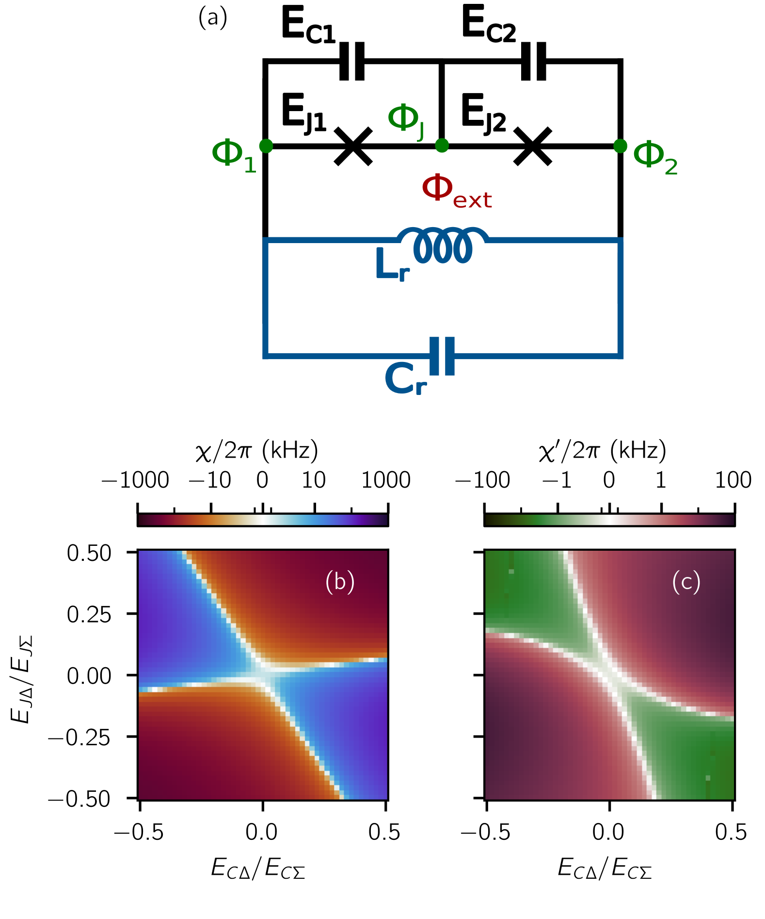
Figure 3: (a) Circuit diagram of the Cooper pair transistor. Symlog colormaps of numerically calculated dispersive shift (b) and Kerr shift (c) with $E_{C_{r}}=2\pi\times$10\text{\,}\mathrm{GHz}$$, $E_{L_{r}}=2\pi\times$100\text{\,}\mathrm{GHz}$$, $E_{J\Sigma}=E_{J1}+E_{J2}=2\pi\times$18\text{\,}\mathrm{GHz}$$, $E_{C\Sigma}=E_{C1}+E_{C2}=2\pi\times$10\text{\,}\mathrm{GHz}$$. With these parameters the resonator frequency is $\omega_{r}\approx 2\pi\times$63\text{\,}\mathrm{GHz}$$ while the qubit frequency is $\omega_{q}\sim 2\pi\times$5\text{\,}\mathrm{GHz}$$.

Our first example is a minimal circuit implementation of the mixed-coupling Hamiltonian shown in Fig. 3(a). In the Cooper-pair box limit, the qubit-resonator coupling in this circuit contains the two terms in Eq. (2), see also Appendix C for the full derivation and the complete expression. Thus, we obtain the Hamiltonian

$$\mathcal{H}_{\text{coupling}}\sim\frac{E_{C\Delta}|z|}{2\epsilon}n_{\delta}\sigma_{x}+\frac{E_{J\Delta}}{|z|}\delta\sigma_{y}~,$$ (9)

where $n_{\delta}$ is the number of photons in the resonator, $\delta$ is its conjugated variable,

$$z=-\cos\frac{\varphi_{ext}}{2}+i\frac{E_{J\Delta}}{E_{J\Sigma}}\sin\frac{\varphi_{ext}}{2}~,$$ (10)

$$m=\frac{E_{CI}n_{g}^{\prime}}{2E_{J\Sigma}}~,\quad\epsilon=\sqrt{m^{2}+|z|^{2}}~,$$ (11)

$n_{g}^{\prime}$ is the qubit offset charge, and $\varphi_{ext}$ is the external flux. The remaining parameters are related to the circuit parameters shown in Fig. 3(a) as

$$E_{J\Sigma}=E_{J1}+E_{J2}~,\quad E_{C\Sigma}=E_{C1}+E_{C2}~,$$ (12)

$$E_{J\Delta}=E_{J1}-E_{J2}~,\quad E_{C\Delta}=E_{C1}-E_{C2}~.$$ (13)

From Eq. (9), we conclude that the imbalances of the capacitive and Josephson energies of the qubit, $E_{C\Delta}$ and $E_{J\Delta}$, play the same role as $g_{X}$ and $g_{P}$.

To verify the influence of the additional coupling terms in Eq. (63) and higher qubit states, we compute the dispersive and Kerr shifts numerically using the Python package scQubits [40]. Since some of the coupling terms in Eq. (63) are as large as the qubit frequency ($\omega_{q}\sim E_{J\Sigma}$), we fix a large resonator frequency $\omega_{r}\gg\omega_{q}$ to stay in the perturbative regime. This choice is made to illustrate a mixed coupling in a circuit realization, and we devote Sec. III.2 for realistic circuit simulations. In Fig. 3 (b), we demonstrate the suppression of the dispersive shift by tuning $E_{C\Delta}$ and $E_{J\Delta}$ despite the additional complexity of the circuit Hamiltonian. Moreover, the nonlinear readout remains possible since the Kerr shift remains nonzero, as shown in Fig. 3(c).

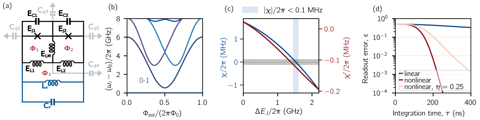
Figure 4: (a) Circuit diagram of a fluxonium molecule (in black) galvanically connected to a readout resonator (in blue). For all circuit simulations, $\Phi_{3}=0$. (b) Numerically simulated energy spectrum of an asymmetric fluxonium molecule with the following energy parameters: $E_{J1}/2\pi=3.63$ GHz,$E_{J2}/2\pi=5.17$ GHz, $E_{L1}=E_{L2}=E_{LM}=2\pi\times 1.2$ GHz, $E_{C1}/2\pi=3.08$ GHz, $E_{C2}/2\pi=2.52$ GHz. $\Phi_{\text{ext}}=(\Phi_{1}+\Phi_{2})/2$. The four nodes of the fluxonium are capacitively coupled to ground with $C_{g1}=C_{g2}=C_{g3}=C_{g4}=0.1$ fF. (c) Numerical simulations of $\chi$ and $\chi^{\prime}$ at $\Phi_{\text{ext}}/(2\pi\Phi_{0})=0.5$ as a function of the energy difference between the two Josephson junctions $\Delta E_{J}=E_{J1}-E_{J2}$. The circuit parameters are the same as in (b) with $E_{J1}=E_{J2}/2\pi=4.4$ GHz when $\Delta E_{J}=0$. The area shaded in blue indicates regions where $|\chi|/2\pi<0.1$ MHz, which gives rise to at worst $T_{\phi,\text{linear}}=1.1$ ms using $\kappa/2\pi=3$ MHz and $T_{\text{eff}}=65$ mK. (d) Readout error with $\chi^{\prime}/2\pi=0.12$ MHz. The pink line is plotted with the same $\chi^{\prime}$ but with quantum efficiency $\eta$ = 0.25. For comparison, the blue line shows readout error with only $\chi/2\pi=0.12$ MHz and perfect quantum efficiency. We use $n_{\text{steady}}=15$ and $\kappa/2\pi=3$ MHz.

III.2 Fluxonium molecule

The Cooper pair transistor, in the described charging limit, is convenient to understand as it is readily modeled as two-level system with well-understood eigenstates. However, the sensitivity to charge noise means that it is unlikely to serve as a technologically relevant platform. To avoid detrimental charge noise while retaining a low-lying pair of computational qubit states, we inductively shunt the island to form a fluxonium molecule [41]. Specifically, we add the three inductive elements to the circuit as shown in Fig. 4(a). The fluxonium molecule operates in a regime of $E_{J}>E_{L}$. Thus, the inductive elements should be in the so-called superinductor regime [42]. What’s more, the charging energy is also larger compared to that of typical single fluxoniums. The fluxonium molecule can be understood as two individual fluxonium qubits that are strongly coupled near $\Phi_{ext}=(\Phi_{1}+\Phi_{2})/2=0.5\Phi_{0}$. At this flux bias, the two lowest-energy states are well separated in energy from the remaining of the energy spectrum, see Fig. 4(b). The resulting ground and first excited states are even and odd superpositions of current flowing in opposite directions in their corresponding loops. The energy spectrum shows high-level transitions in the bandwidth of typical readout frequencies of $5$ to $8$ GHz. For fluxonium qubits, it is well-studied how these higher excited states contribute to the dispersive shift [43, 31]. Similarly, for the fluxonium molecule, the higher excited states will impact both the dispersive shift and the Kerr shift; thus, the full spectrum must be considered in the calculation of the circuit properties.

Here, we compute the dispersive and Kerr shifts numerically with realistic circuit parameters; see the Zenodo repository [44] for the code. Similarly to the Cooper pair transistor, the imbalance in capacitive and inductive coupling provides the means to suppress the dispersive shift. As a concrete example, we show in Fig. 4(c) that as we increase the imbalance in the two Josephson energies, we reach a point where $\chi$ goes to zero while we obtain $\chi^{\prime}/2\pi\approx-0.1$ MHz. For these calculations, we have $\omega_{q}=107$ MHz and $\omega_{r}=6.15$ GHz with a resonator impedance of $100~\Omega$, and resonator anharmonicity $K_{r}/2\pi=0.58$ MHz. We note that the somewhat high resonator impedance helps in achieving a larger $\chi^{\prime}$ without increasing the self-Kerr of the resonator too much, see also Appendix D for more details. In Fig. 4(c), we present the actual energy difference between the two Josephson junctions in units of GHz to indicate a window of $|\chi/2\pi|<0.1$ MHz. This window corresponds to around $0.1$ GHz of $\Delta E_{J}$, while $\chi^{\prime}$ maintains non-zero at around $-0.12$ MHz. In other words, we allow for a relative precision of 2.5% in the junction energies. Although such precision is challenging on a wafer-scale, the junctions for a specific fluxonium molecule are likely to be located within small windows where spread in junction energies below 2% has been demonstrated [45].

Taking the values of $\chi$ and $\chi^{\prime}$ given by the circuit simulations as shown in Fig. 4(c), we perform time-domain readout simulations as outlined in Section II.2. Setting $n_{\text{steady}}=15$, we obtain readout fidelities as shown in Fig. 4(d) where the readout error goes below $10^{-4}$ within $300$ ns assuming perfect measurement efficiency. For a more realistic value of the measurement efficiency of 25%, we still obtain a measurement error below $10^{-3}$ within $400$ ns. Note that in Fig. 4(d), we also plot the readout fidelity contribution from a small $\chi$ set to the same value obtained for $\chi^{\prime}$ in the circuit simulations. The linear dispersive readout, however, has low fidelity. Similarly, when both the linear and nonlinear cases are included, the results do not differ notably from the purely nonlinear readout.

For the simulations here to be valid, it is important to verify that we are still operating within a dispersive regime of the readout. In other words, the steady-state photon number must be below the critical photon number ($n_{\text{crit}}$), which is usually designated as the photon number at which the dressed qubit states are equal superpositions of the original qubit states [6]. For multi-level systems, this is more complicated and requires accounting of higher order transitions [46, 47, 48]. To estimate the critical photon number of the circuit in Fig. 4(a) and to take into account the influence of higher-order transitions, we calculate the overlap in the fluxonium molecule degree of freedom between dressed states $\ket{q,0}$ and $\ket{q^{\prime},n}$, where $q=\{0,1\}$, $q^{\prime}=\{1,2,3,4,5,6\}$ refer to the fluxonium molecule excitations and $n$ refers to resonator photon number. For photon numbers below 25, we do not observe hybridization of any qubit state with any higher level above an overlap level of 0.05, and overlaps do not exceed 0.1 until photon numbers above 60. These statements remain true whether the circuit is balanced or imbalanced. The detailed results for this calculation can be found in Appendix E.1. We conclude that imbalancing the fluxonium molecule to achieve suppression of $\chi$ does not decrease $n_{\text{crit}}$ and that $\bar{n}\leq 15$ appears to be below the estimated critical regime.

Our results indicate that, despite the complexity of this fluxonium molecule circuit and the deviation from a perfect two-level circuit behavior, we can still use a mixed-coupling architecture to implement our nonlinear readout scheme with minimal residual shot-noise dephasing.

IV Conclusion & Outlook

We considered a ‘mixed’ spin-boson coupling regime, which refers to the simultaneous presence of bilinear couplings of non-commuting quadratures of the spin and boson being paired. We showed that in this regime it is possible to suppress the dispersive shift while maintaining a nonzero nonlinear qubit-state dependent shift, the Kerr shift. In the absence of linear response, the photon shot noise dephasing rate scales $\sim\bar{n}_{th}^{3}$ and is therefore reduced when $\bar{n}_{th}\ll 1$. Given this improvement, we proposed a nonlinear readout scheme in which we probe the Kerr shift.

Next, we demonstrated the implementation of a mixed coupling Hamiltonian in two superconducting quantum circuits: a Cooper pair transistor and a fluxonium molecule. Our circuit implementations achieve the desired coupling terms by changing the imbalance of the capacitive and Josephson energies of the lumped elements in the qubit. The fluxonium molecule instance shows that mixed coupling concept for non-simultanousely suppressing $\chi$ and $\chi^{\prime}$ works beyond the two-level approximation. Finally, with experimentally realistic parameters and readout power within the dispersive limit, we illustrated using the fluxonium molecule that this readout scheme can be used to achieve high-fidelity readout with suppression of residual photon shot noise. A possible experimental challenge in implementing the fluxonium molecule circuit for nonlinear readout is the flux crosstalk. Further work could explore possible circuits in which a single-mode qubit is coupled to the readout resonator with mixed coupling.

Finally, we consider another application of our concept: the spin serving as ancilla for the bosonic mode, which can serve as a quantum memory [49, 50, 51]. One of the principal issues of such architectures is the reciprocal problem of the one described here: spin errors are inherited as uncorrectable errors in the boson. Because the leading-order interaction is typically the dispersive shift $\chi$, $T_{1}$-type spin errors are inherited as uncorrectable bosonic dephasing, which is concurrently precisely the noise channel that such cavities without qubits are meant to be biased against [52, 53] To combat this, various quantum control approaches have been developed to use reduced values of $\chi$ [54, 55]. Our concept suggests an alternative approach, whereby linear bosonic dephasing is reduced by nullifying $\chi$ entirely while accomplishing quantum control through the Kerr shift interaction. We leave a technical evaluation of this idea for future work.

Author contributions

V.F. initiated the project. V.F. and A.L.R.M. developed the theory of dispersive shift suppression in a two-level system. C.K.A. and V.F. proposed using mixed-coupling for nonlinear readout. All authors contributed to the design of the circuit implementations and A.L.R.M., J.H., and A.M. performed the circuit simulations. J.H., T.S., and C.K.A. performed the readout simulations. J.H., A.L.R.M., C.K.A., and V.F. wrote the manuscript.

Appendix A Perturbation theory on the mixed-coupling Hamiltonian

We perform a Schrieffer-Wolff transformation on the Hamiltonian from Eq. (1) symbolically. The code to reproduce our calculations is available in [44]. The leading-order correction to the Hamiltonian:

$$\delta H=\hbar\frac{1}{\omega_{r}^{2}-\omega_{q}^{2}}\left[\omega_{r}g_{P}g_{X}(X^{2}+P^{2})+\omega_{q}(g_{P}^{2}P^{2}-g_{X}^{2}X^{2})\right]\sigma_{z}~.$$ (14)

Note that the couplings $g_{X}$ and $g_{P}$ result in qubit-state-dependent corrections to the inductance $\sim X^{2}$ and capacitance $\sim P^{2}$ of the resonator. From Eq. (14), we extract the dispersive shift by collecting the terms proportional to $a^{\dagger}a\sigma_{z}$, resulting in the expression shown in Eq. (3). We can find the roots of Eq. (3) analytically, giving the following relation between $g_{P}$ and $g_{X}$:

$$g_{P}=\frac{g_{X}}{\omega_{q}}\left(\omega_{r}\pm\sqrt{\omega_{r}^{2}-\omega_{q}^{2}}\right)~.$$ (15)

In Fig. 1 (b, c), we show the resulting dispersive and Kerr shifts from a symbolic Schrieffer-Wolff transformation up to the next-leading-order correction. Our expression for $\chi=0$ in Eq. (15) still holds since we are deep in the perturbative regime, and therefore, the next-leading-order corrections to $\chi$ are negligible (note that $\chi^{\prime}/\chi\ll 1$). However, the full expressions are available in [44].

Appendix B Dephasing rate due to $\chi^{\prime}$

References [29] and [56] both investigated qubit dephasing into the a thermal resonator. However, in both works, only the linear dispersive shift is considered. Here we derive the qubit dephasing rate due to coupling term $\chi^{\prime}\sigma_{z}\hat{a}^{\dagger}\hat{a}^{\dagger}\hat{a}\hat{a}$ using a similar approach as used in [56].

We consider the following dispersive Hamiltonian

$$\frac{H}{\hbar}=\omega_{r}\hat{a}^{\dagger}\hat{a}+\left(\chi^{\prime}_{0}\ket{0}\bra{0}+\chi^{\prime}_{1}\ket{1}\bra{1}\right)\hat{a}^{\dagger}\hat{a}^{\dagger}\hat{a}\hat{a}+\tilde{\omega}_{q}\ket{1}\bra{1},$$ (16)

where $\tilde{\omega}_{q}$ is the Lamb shifted qubit frequency, $\chi^{\prime}_{0}$ and $\chi^{\prime}_{1}$ are the qubit state-dependent shifts on the resonator anharmonicity. Here we only investigate qubit dephasing due to thermal photons so we assume there is no active driving through the resonator. We describe the effects of having thermal photon populations in the resonator with the master equation

$$\dot{\rho} =-\frac{i}{\hbar}[H,\rho]+\kappa(n_{\text{th}}+1)\mathcal{D}[\hat{a}]\rho+\kappa n_{\text{th}}\mathcal{D}[\hat{a}^{\dagger}]\rho,$$ (17)

where $\mathcal{D}[\hat{\mathcal{L}}]\rho=(2\mathcal{\hat{L}}\rho\mathcal{\hat{L}}^{\dagger}-\mathcal{\hat{L}}^{\dagger}\mathcal{\hat{L}}\rho-\rho\mathcal{\hat{L}}^{\dagger}\mathcal{\hat{L}})/2$ is the superoperator that describes the effect of dissipation, $\kappa$ is the linewidth of the resonator, and $n_{\text{th}}$ is the thermal photon number in the resonator.

We decompose the system to write the qubit-resonator density matrix as

$$\rho =\rho^{11}\ket{1}\bra{1}+\rho^{00}\ket{0}\bra{0}+\rho^{10}\ket{1}\bra{0}+\rho^{01}\ket{0}\bra{1},$$ (18)

where $\rho^{xy}$ only acts in the resonator Hilbert space. Substituting Eqs (16) and (18) into the master equation, and moving to the qubit rotating frame, we get

$$\dot{\rho}^{11} =\kappa(n_{\text{th}}+1)\mathcal{D}[\hat{a}]\rho^{11}+\kappa n_{\text{th}}\mathcal{D}[\hat{a}^{\dagger}]\rho^{11}-i\omega_{r}[\hat{a}^{\dagger}\hat{a},\rho^{11}]-i\chi_{1}^{\prime}[\hat{a}^{\dagger}\hat{a}^{\dagger}\hat{a}\hat{a},\rho^{11}],$$ (19)

$$\dot{\rho}^{00} =\kappa(n_{\text{th}}+1)\mathcal{D}[\hat{a}]\rho^{00}+\kappa n_{\text{th}}\mathcal{D}[\hat{a}^{\dagger}]\rho^{00}-i\omega_{r}[\hat{a}^{\dagger}\hat{a},\rho^{11}]-i\chi_{0}^{\prime}[\hat{a}^{\dagger}\hat{a}^{\dagger}\hat{a}\hat{a,}\rho^{11}],$$ (20)

$$\dot{\rho}^{10} =\kappa(n_{\text{th}}+1)\mathcal{D}[\hat{a}]\rho^{10}+\kappa n_{\text{th}}\mathcal{D}[\hat{a}^{\dagger}]\rho^{10}-i\omega_{r}[\hat{a}^{\dagger}\hat{a},\rho^{10}]+i\chi_{0}^{\prime}\rho^{10}\hat{a}^{\dagger}\hat{a}^{\dagger}\hat{a}\hat{a}-i\chi_{1}^{\prime}\hat{a}^{\dagger}\hat{a}^{\dagger}\hat{a}\hat{a}\rho^{10},$$ (21)

and $\rho^{01}=(\rho^{10})^{*}$.

To solve the differential equations above we express the density matrix using the positive-P representation [57]:

$$\rho=\int d^{2}\alpha\int d^{2}\beta\frac{|\alpha\rangle\langle\beta^{*}|}{\langle\beta^{*}|\alpha\rangle}P(\alpha,\beta)~,$$ (22)

and use the identities

$$\hat{a}\frac{|\alpha\rangle\langle\beta^{*}|}{\langle\beta^{*}|\alpha\rangle}=\alpha\frac{|\alpha\rangle\langle\beta^{*}|}{\langle\beta^{*}|\alpha\rangle}~,\quad\quad\hat{a}^{\dagger}\frac{|\alpha\rangle\langle\beta^{*}|}{\langle\beta^{*}|\alpha\rangle}=(\beta+\partial_{\alpha})\frac{|\alpha\rangle\langle\beta^{*}|}{\langle\beta^{*}|\alpha\rangle}~,$$ (23)

$$\frac{|\alpha\rangle\langle\beta^{*}|}{\langle\beta^{*}|\alpha\rangle}\hat{a}^{\dagger}=\beta\frac{|\alpha\rangle\langle\beta^{*}|}{\langle\beta^{*}|\alpha\rangle}~,\quad\quad\frac{|\alpha\rangle\langle\beta^{*}|}{\langle\beta^{*}|\alpha\rangle}\hat{a}=(\alpha+\partial_{\beta})\frac{|\alpha\rangle\langle\beta^{*}|}{\langle\beta^{*}|\alpha\rangle}~.$$ (24)

By applying these identities to Eq. (22), using partial integration and assuming that the boundary terms vanish ($P(\pm\infty,\pm\infty)=0$), we obtain the following correspondences [57]:

$$\hat{a}\rho\leftrightarrow\alpha P(\alpha,\beta)~,\quad\hat{a}^{\dagger}\rho\leftrightarrow(\beta-\partial_{\alpha})P(\alpha,\beta)~,\quad\rho\hat{a}^{\dagger}\leftrightarrow\beta P(\alpha,\beta)~,\quad\rho\hat{a}\leftrightarrow(\alpha-\partial_{\beta})P(\alpha,\beta)~.$$ (25)

Since we want to determine the qubit dephasing rate, we focus only on the $\rho^{10}$ differential equation. The positive-P representation of Eq. (21) gives

$$\dot{P}^{10} =\partial_{\alpha}[(i\omega_{r}+\kappa/2)\alpha P^{10}]+\partial_{\beta}[(-i\omega_{r}+\kappa/2)\beta P^{10}]+\kappa n_{\text{th}}\partial^{2}_{\alpha,\beta}P^{10}$$

$$\quad+i\chi^{\prime}_{0}(\alpha^{2}-2\alpha\partial_{\beta}-\partial^{2}_{\beta})\beta^{2}P^{10}-i\chi^{\prime}_{1}(\beta^{2}-2\beta\partial_{\alpha}-\partial^{2}_{\alpha})\alpha^{2}P^{10}~.$$ (26)

To solve this differential equation, we introduce the transformation

$$P(\alpha,\beta)=\int da\int db\bar{P}(a,b)e^{ia\alpha+ib\beta+c.c}~,$$ (27)

which leads to the identities:

$$\partial_{\alpha}P(\alpha,\beta) =\int da\int db\,(ia)\overline{P}(a,b)e^{ia\alpha+ib\beta+\text{c.c.}},$$ (28)

$$\partial_{\beta}P(\alpha,\beta) =\int da\int db\,(ib)\overline{P}(a,b)e^{ia\alpha+ib\beta+\text{c.c.}},$$ (29)

$$\alpha P(\alpha,\beta) =\int da\int db\,(i)\partial_{a}\overline{P}(a,b)e^{ia\alpha+ib\beta+\text{c.c.}},$$ (30)

$$\beta P(\alpha,\beta) =\int da\int db\,(i)\partial_{b}\overline{P}(a,b)e^{ia\alpha+ib\beta+\text{c.c.}}.$$ (31)

The resulting differential equation for $\bar{P}^{10}(a,b)$ after the transformation is:

$$\partial_{t}\bar{P}^{10} =\kappa/2(-a\partial_{a}-b\partial_{b})\bar{P}^{10}+i\omega_{r}(-a\partial_{a}+b\partial_{b})\bar{P}^{10}-\kappa n_{\text{th}}ab\bar{P}^{10}$$

$$\quad+i\chi^{\prime}_{0}[(\partial_{a,b}^{2})^{2}-2b(\partial_{b})^{2}\partial_{a}-b^{2}(\partial_{b})^{2}]\bar{P}^{10}-i\chi^{\prime}_{1}[(\partial_{a,b}^{2})^{2}-2a(\partial_{a})^{2}\partial_{b}-a^{2}(\partial_{a})^{2}]\bar{P}^{10}.$$ (32)

By assuming a Gaussian distribution for $\bar{P}^{10}(a,b)$, and only considering thermal driving, we can write

$$\bar{P}^{10}(a,b)=e^{i\mu}e^{-abZ/2}~,$$ (33)

which gives

$$\dot{\mu} =-\chi^{\prime}Z^{2},$$ (34)

$$\dot{Z} =-2i\chi^{\prime}(Z^{3}+2Z^{2})-\kappa Z+2\kappa n_{\text{th}},$$ (35)

where $\chi^{\prime}=(\chi^{\prime}_{1}-\chi^{\prime}_{0})/2$.

The resonator-induced dephasing rate($\Gamma$) and frequency shift ($\Delta$) are related to $\mu$ through

$$e^{i\mu}=e^{-\int^{t}_{0}(\Gamma+i\Delta)dt}.$$ (36)

Moreover, with Eq. (34), we get

$$\Gamma=\text{Im}(\mu) =-\chi^{\prime}\text{Im}(Z^{2}),$$ (37)

$$\Delta=\text{Re}(\mu) =-\chi^{\prime}\text{Re}(Z^{2}),$$ (38)

We solve Eq. (35) numerically with physically realistic values of $\kappa$, $n_{\text{th}}$, and $\chi^{\prime}$ and find that $\text{Im}(Z),\text{Re}(Z)\ll 1$. Thus, we drop the terms $\mathcal{O}(Z^{3})$, resulting on the differential equation

$$\dot{Z} =-4i\chi^{\prime}Z^{2}-\kappa Z+2\kappa n_{\text{th}},$$ (39)

which has an analytical solution

$$Z=\frac{i}{8\chi^{\prime}}(\kappa-A\tanh{(tA/2}+B))~,$$ (40)

where

$$A=\sqrt{\kappa^{2}+32i\kappa n_{\text{th}}\chi^{\prime}}~,\quad B=\arctan\left[\frac{\kappa+16\chi^{\prime}\kappa n_{\text{th}}/(\kappa-4i\chi^{\prime})}{A}\right].$$ (41)

Finally, because $\tanh{(tA/2+B)}\approx 1$,

$$Z=\frac{i}{8\chi^{\prime}}(\kappa-\sqrt{\kappa^{2}+32i\kappa n_{\text{th}}\chi^{\prime}}).$$ (42)

Finally, assuming $\kappa/\chi^{\prime}\gg 8\sqrt{2}n_{\text{th}}$, we expand the square root to second order in a Taylor series and obtain the formula for qubit dephasing rate due to non-linear coupling to the resonator

$$\Gamma=\frac{64n_{\text{th}}^{3}(\chi^{\prime})^{2}}{\kappa}.$$ (43)

For superconducting qubit readout, we have $n_{\text{th}}\ll 0.1$, which means that with an additional condition of $\kappa/\chi^{\prime}>1$, we recover the same approximation needed to obtain the formula above.

Appendix C Mixed-coupling with a Cooper pair transistor

The circuit depicted in Fig. 3 has a Lagrangian $L=T-U$ with

$$T =\frac{1}{2}C\left(\dot{\phi}_{2}-\dot{\phi}_{1}\right)^{2}+\frac{1}{2}C_{J1}\left(\dot{\phi}_{J}-\dot{\phi}_{1}\right)^{2}+\frac{1}{2}C_{J2}\left(\dot{\phi}_{J}-\dot{\phi}_{2}\right)^{2}~,$$ (44)

$$U =\frac{1}{2L}\left(\phi_{2}-\phi_{1}-\phi_{ext}\right)^{2}-E_{J1}\cos\left(\varphi_{J}-\varphi_{1}\right)-E_{J2}\cos\left(\varphi_{J}-\varphi_{2}\right)~.$$ (45)

Assuming the inductance is small, $\varphi_{2}-\varphi_{1}=\varphi_{ext}+\delta$, and defining the island mode phase $\varphi_{I}=\varphi_{J}-\frac{1}{2}(\varphi_{1}+\varphi_{2})$,

$$T =\frac{1}{2}C\dot{\delta}^{2}+\frac{1}{2}C_{J1}\left(\dot{\phi}_{I}+\frac{1}{2}\dot{\delta}\right)^{2}+\frac{1}{2}C_{J2}\left(\dot{\phi}_{I}-\frac{1}{2}\dot{\delta}\right)^{2}$$ (46)

$$U =\frac{\varphi_{0}^{2}}{2L}\delta^{2}-E_{J\Sigma}\cos\frac{\varphi_{ext}+\delta}{2}\cos\varphi_{I}-E_{J\Delta}\sin\frac{\varphi_{ext}+\delta}{2}\sin\varphi_{I}$$ (47)

Finally, we arrive at the Hamiltonian $H=T+U$, where

$$T =E_{C\delta}n_{\delta}^{2}+E_{CI}(n_{I}-n_{g})^{2}-E_{C\Delta}n_{\delta}(n_{I}-n_{g})$$ (48)

$$U =\frac{\varphi_{0}^{2}}{2L}\delta^{2}-E_{J\Sigma}\cos\frac{\varphi_{ext}+\delta}{2}\cos\varphi_{I}+E_{J\Delta}\sin\frac{\varphi_{ext}+\delta}{2}\sin\varphi_{I}$$ (49)

with

$$E_{C\delta}=\frac{e^{2}}{2}\frac{C_{J1}+C_{J2}}{\det(\mathbf{C})}~,\quad E_{CI}=\frac{e^{2}}{2}\frac{C+\frac{1}{4}(C_{J1}+C_{J2})}{\det(\mathbf{C})}~,\quad E_{C\delta} =\frac{e^{2}}{2}\frac{(C_{J1}-C_{J2})}{\det(\mathbf{C})}$$ (50)

and

$$\mathbf{C} =\begin{pmatrix}C+\frac{1}{4}(C_{J1}+C_{J2})&\frac{1}{2}(C_{J1}-C_{J2})\\ \frac{1}{2}(C_{J1}-C_{J2})&C_{J1}+C_{J2}\end{pmatrix}~.$$ (51)

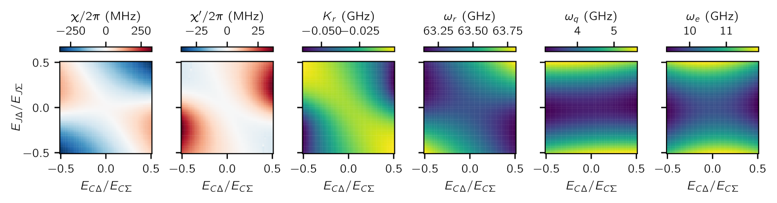
Figure 5: A more detailed simulation result showing the change of $\chi$, $\chi^{\prime}$, $K_{r}$, $\omega_{r}$, $\omega_{q}$, and the transition frequency of the Cooper pair transistor from the ground state to the second excited state $\omega_{e}$ as a function of the capacitance and Josephson energy imbalances.

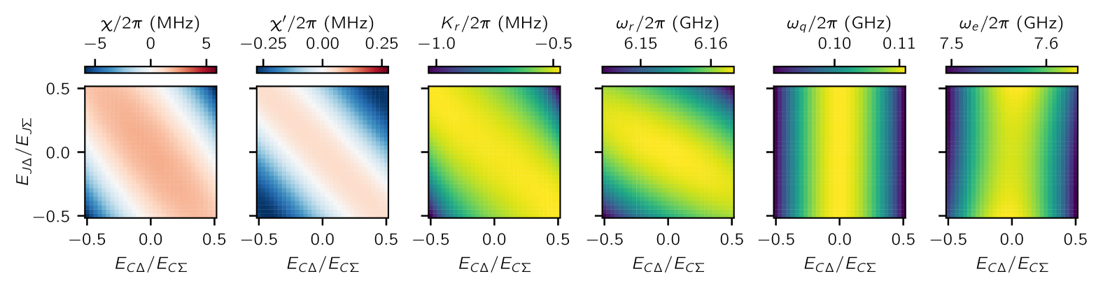
Figure 6: A more detailed simulation result showing the change of $\chi$, $\chi^{\prime}$, $K_{r}$, $\omega_{r}$, $\omega_{q}$, and the transition frequency of the fluxonium molecule from the ground state to the second excited state $\omega_{e}$ as a function of the capacitance and Josephson energy imbalances.

C.0.1 Cooper Pair Box limit

In the Cooper pair box limit, we make the substitutions:

$$n_{I}-n_{g} \rightarrow\frac{1}{2}(\sigma_{z}-n_{g}^{\prime})~,\quad\cos(\varphi_{I})\rightarrow\sigma_{x}~,\quad\sin(\varphi_{I})\rightarrow\sigma_{y}$$ (52)

so that the kinetic and potential terms of the Hamiltonian now read

$$T =E_{C\delta}n_{\delta}^{2}+\frac{1}{2}E_{CI}n_{g}^{\prime}\sigma_{z}-\frac{1}{2}E_{C\Delta}n_{\delta}(\sigma_{z}-n_{g}^{\prime})$$ (53)

$$U =\frac{\varphi_{0}^{2}}{2L}\delta^{2}-E_{J\Sigma}\cos\frac{\varphi_{ext}+\delta}{2}\sigma_{x}+E_{J\Delta}\sin\frac{\varphi_{ext}+\delta}{2}\sigma_{y}$$ (54)

We now Taylor expand $U$ with respect to $\delta$

$$U\approx ~\frac{\varphi_{0}^{2}}{2L}\delta^{2}-E_{J\Sigma}\cos\frac{\varphi_{ext}}{2}\sigma_{x}+E_{J\Delta}\sin\frac{\varphi_{ext}}{2}\sigma_{y}+\frac{\delta}{2}\left(E_{J\Sigma}\sin\frac{\varphi_{ext}}{2}\sigma_{x}+E_{J\Delta}\frac{\delta}{2}\cos\frac{\varphi_{ext}}{2}\sigma_{y}\right)$$ (55)

$$+\frac{\delta^{2}}{8}\left(E_{J\Sigma}\cos\frac{\varphi_{ext}}{2}\sigma_{x}-E_{J\Delta}\sin\frac{\varphi_{ext}}{2}\sigma_{y}\right)~.$$

Using the definitions from Eq. (11), we rewrite the full Hamiltonian as

$$\mathcal{H} =\mathcal{H}_{osc}+\mathcal{H}_{I}+V$$ (56)

$$\mathcal{H}_{osc} =E_{C\delta}n_{\delta}^{2}-\frac{1}{2}E_{C\Delta}n_{\delta}+\frac{\varphi_{0}^{2}}{2L}\delta^{2}$$ (57)

$$\mathcal{H}_{I} =E_{J\Sigma}\left(m\sigma_{z}+z\sigma_{+}+z^{*}\sigma_{-}\right)$$ (58)

$$V =-\frac{1}{2}E_{C\Delta}n_{\delta}\sigma_{z}-\delta\left(\gamma\sigma_{+}+\gamma^{*}\sigma_{-}\right)$$ (59)

and diagonalize the island modes via

$$R =\sqrt{\frac{|z|^{2}}{2\epsilon}}\left(\begin{matrix}-\frac{\sqrt{\epsilon-m}}{z^{*}}&\frac{\sqrt{\epsilon+m}}{z^{*}}\\ \frac{1}{\sqrt{\epsilon-m}}&\frac{1}{\sqrt{\epsilon+m}}\end{matrix}\right)\quad\Rightarrow\quad R^{\dagger}\mathcal{H}_{I}R=E_{J\Sigma}\epsilon\sigma_{z}~.$$ (60)

the couplings $V$ in the new basis take the form:

$$V =V_{z}+V_{od}~,$$ (61)

$$V_{z} =\left(\frac{E_{C\Delta}E_{CI}}{4E_{J\Sigma}\epsilon}n_{g}^{\prime}n_{\delta}+\frac{E_{J\Sigma}^{2}+E_{J\Delta}^{2}}{4E_{J\Sigma}\epsilon}\sin\varphi_{ext}\delta+\frac{1}{4}E_{J\Sigma}\frac{|z|^{2}}{\epsilon}\delta^{2}\right)\sigma_{z}~,$$ (62)

$$V_{od} =\frac{E_{C\Delta}|z|}{2\epsilon}n_{\delta}\sigma_{x}-\frac{E_{CI}(E_{J\Sigma}^{2}-E_{J\Delta}^{2})}{4E_{J\Sigma}}\frac{n_{g}^{\prime}}{\epsilon|z|}\sin\varphi_{ext}\delta\sigma_{x}+\frac{E_{J\Delta}}{|z|}\delta\sigma_{y}+\frac{1}{4}E_{J\Sigma}\frac{|z|m}{\epsilon}\delta^{2}\sigma_{x}~.$$ (63)

From this expression, we notice the presence of the targeted couplings written in Eq. (9).

Appendix D Detailed circuit simulation results

Here we provide additional numerical simulations of the circuits shown in Fig. 3(a) and Fig. 4(a). We repeat the dispersive and Kerr shift plots from the main text and additionally show the Kerr shift of the resonator $K_{r}$ and the frequencies of the resonator ($\omega_{r}$), qubit ($\omega_{q}$), and first excited state in the qubit ($\omega_{e}$). This fact that there are no sudden jumps in these energies demonstrates that the qubit dispersive and Kerr shifts are suppressed due to the mixed coupling rather than qubit and the resonator level crossings. Additionally, we show that the Kerr shift of the resonator remains finite.

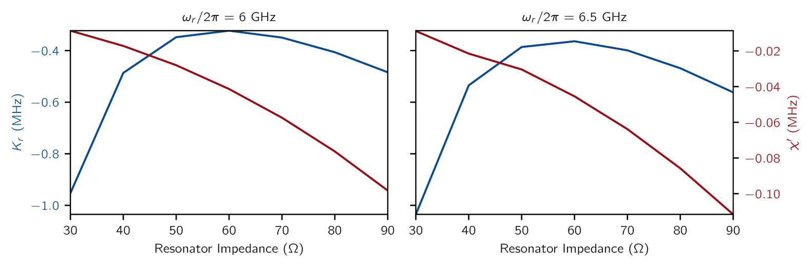
Figure 7: Resonator self-Kerr $K_{r}$ and Kerr shift $\chi^{\prime}$ as a function of resonator impedance for fixed resonator frequency of $6$ GHz (a) and $6.5$ GHz (b). The fluxonium molecule parameters are the same as in Fig. 4(c). The Josephson energies are imbalanced to find regions where $\chi$ is supprressed. All $\chi^{\prime}$ values presented here correspond to when $|\chi|/2\pi$ is suppressed to be below $0.2$ MHz.

As we search for a set of realistic circuit parameters for the fluxonium molecule circuit, we find that for a wide choice of qubit parameters, independent suppression of $\chi$ and $\chi^{\prime}$ can be found. However, some resonator impedance engineering is needed to suppress $K_{r}$ while keeping $\chi^{\prime}$ high enough. In Fig. 7 we see that for the circuit in Fig. 4(a), $|K_{r}|$ has a local minimum at around $50~\Omega$, whereas $|\chi^{\prime}|$ increases with resonator impedance. This motivates our choice of the relatively high resonator impedance in the main text.

Appendix E Readout performance

E.1 Dispersive regime validation

With the exact diagonalization results of the full circuit Hamiltonian obtained from ScQubits simulation, we label the dressed eigenstates as $\ket{q,n}$ and calculate the overlap of the qubit degree of freedom between states $\ket{q,0}$ and $\ket{q^{\prime},n}$ for possible qubit transition $i-j$. More concretely, we calculate the fidelity between $\text{Tr}_{res}\rho_{\ket{q,0}}$ and $\text{Tr}_{res}\rho_{\ket{q^{\prime},n}}$ as a function of resonator photon number $n$. Fig. 8 (a) shows an unsuppressed $\chi/2\pi$ of $2$ MHz and $\chi^{\prime}/2\pi=0.05$ MHz, where we see no abrupt hybridization until $n\approx 70$. The same trend can be seen for the imbalanced case where $\chi$ is suppressed. Fig. 8 (b) features $\chi/2\pi=-0.02$ MHz and $\chi^{\prime}/2\pi=-0.12$ MHz.

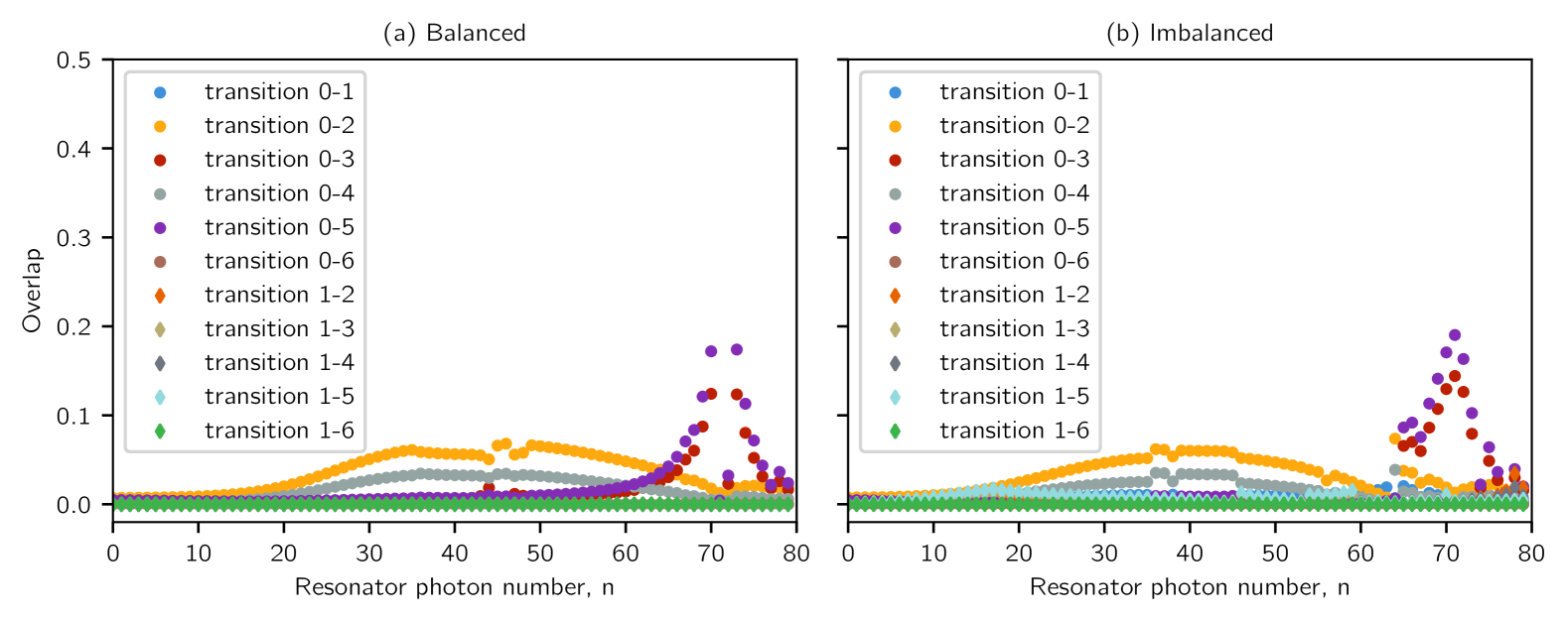
Figure 8: Qubit state overlap as a function of resonator photon number. The balanced one (a) serves as a reference and has the same circuit parameters as in Fig. 4(c) except that the fluxonium molecule is perfectly symmetric (i.e, both the capacitance and the Josephson energy imbalance are zero). The imbalanced one (b) has the same circuit parameter used for the readout simulation in Fig. 4(d).

E.2 Choice of $\kappa$

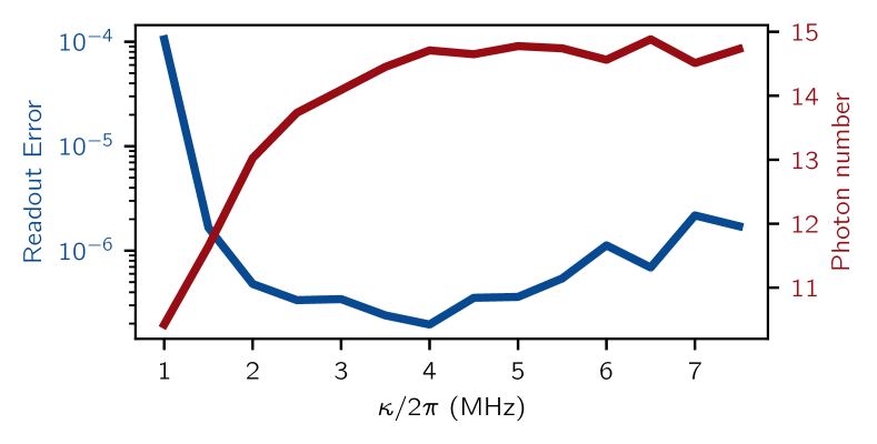
Figure 9: Readout error as a function of readout linewith $\kappa$. Here we use $\chi^{\prime}/2\pi=0.12$ MHz. The integration time is $400$ ns. The photon number is number of photons in the readout reasonator at the end of the $400$ ns readout duration.

Throughout the main text, a readout linewidth of $\kappa/2\pi=3$ MHz is used. We want to clarify our reasons behind this choice, especially in support of our proposal in using the fluxonium molecule circuit as a realization of our readout scheme. First, as can be seen in Fig. 9, the readout error is minimized near $\kappa/2\pi=4$ MHz. Note that the readout error goes below $10^{-4}$ even with a moderate $\kappa/2\pi=1.5$ MHz. However, considering the relatively high $K_{r}$, we did not opt for a particularly low $\kappa$. This also helps suppress Purcell decay.

References

- Nielsen and Chuang [2010] Michael A Nielsen and Isaac L Chuang. Quantum computation and quantum information. Cambridge university press, 2010.
- Preskill [2018] John Preskill. Quantum computing in the nisq era and beyond. Quantum, 2:79, 2018.
- Kjaergaard et al. [2020] Morten Kjaergaard, Mollie E Schwartz, Jochen Braumüller, Philip Krantz, Joel I-J Wang, Simon Gustavsson, and William D Oliver. Superconducting qubits: Current state of play. Annual Review of Condensed Matter Physics, 11(1):369–395, 2020.
- Krantz et al. [2019] Philip Krantz, Morten Kjaergaard, Fei Yan, Terry P Orlando, Simon Gustavsson, and William D Oliver. A quantum engineer’s guide to superconducting qubits. Applied physics reviews, 6(2), 2019.
- Haroche and Raimond [2006] Serge Haroche and J-M Raimond. Exploring the quantum: atoms, cavities, and photons. Oxford university press, 2006.
- Blais et al. [2004] Alexandre Blais, Ren-Shou Huang, Andreas Wallraff, Steven M Girvin, and R Jun Schoelkopf. Cavity quantum electrodynamics for superconducting electrical circuits: An architecture for quantum computation. Physical Review A—Atomic, Molecular, and Optical Physics, 69(6):062320, 2004.
- Blais et al. [2021] Alexandre Blais, Arne L Grimsmo, Steven M Girvin, and Andreas Wallraff. Circuit quantum electrodynamics. Reviews of Modern Physics, 93(2):025005, 2021.
- Chen et al. [2023] Liangyu Chen, Hang-Xi Li, Yong Lu, Christopher W Warren, Christian J Križan, Sandoko Kosen, Marcus Rommel, Shahnawaz Ahmed, Amr Osman, Janka Biznárová, et al. Transmon qubit readout fidelity at the threshold for quantum error correction without a quantum-limited amplifier. npj Quantum Information, 9(1):26, 2023.
- Dassonneville et al. [2020] R Dassonneville, T Ramos, V Milchakov, L Planat, Étienne Dumur, F Foroughi, J Puertas, S Leger, K Bharadwaj, J Delaforce, et al. Fast high-fidelity quantum nondemolition qubit readout via a nonperturbative cross-kerr coupling. Physical Review X, 10(1):011045, 2020.
- Heinsoo et al. [2018] Johannes Heinsoo, Christian Kraglund Andersen, Ants Remm, Sebastian Krinner, Theodore Walter, Yves Salathé, Simone Gasparinetti, Jean-Claude Besse, Anton Potočnik, Andreas Wallraff, et al. Rapid high-fidelity multiplexed readout of superconducting qubits. Physical Review Applied, 10(3):034040, 2018.
- Chen et al. [2012] Yu Chen, D Sank, P O’Malley, T White, R Barends, B Chiaro, J Kelly, E Lucero, M Mariantoni, A Megrant, et al. Multiplexed dispersive readout of superconducting phase qubits. Applied Physics Letters, 101(18), 2012.
- Hinderling et al. [2024] Manuel Hinderling, SC ten Kate, Daniel Zachary Haxell, Marco Coraiola, Stephan Paredes, Erik Cheah, Filip Krizek, Rudiger Schott, Werner Wegscheider, Deividas Sabonis, et al. Flip-chip-based fast inductive parity readout of a planar superconducting island. PRX Quantum, 5(3):030337, 2024.
- Wallraff et al. [2005] Andreas Wallraff, David I Schuster, Alexandre Blais, Luigi Frunzio, Johannes Majer, Michel H Devoret, Steven M Girvin, and Robert J Schoelkopf. Approaching unit visibility for control of a superconducting qubit with dispersive readout. Physical review letters, 95(6):060501, 2005.
- Walter et al. [2017] Theodore Walter, Philipp Kurpiers, Simone Gasparinetti, Paul Magnard, Anton Potočnik, Yves Salathé, Marek Pechal, Mintu Mondal, Markus Oppliger, Christopher Eichler, et al. Rapid high-fidelity single-shot dispersive readout of superconducting qubits. Physical Review Applied, 7(5):054020, 2017.
- Schuster et al. [2005] D. I. Schuster, A. Wallraff, A. Blais, L. Frunzio, R.-S. Huang, J. Majer, S. M. Girvin, and R. J. Schoelkopf. ac stark shift and dephasing of a superconducting qubit strongly coupled to a cavity field. Physical Review Letters, 94(12), March 2005. ISSN 1079-7114. doi: 10.1103/physrevlett.94.123602. URL http://dx.doi.org/10.1103/PhysRevLett.94.123602.
- Gambetta et al. [2006] Jay Gambetta, Alexandre Blais, David I Schuster, Andreas Wallraff, L Frunzio, J Majer, Michel H Devoret, Steven M Girvin, and Robert J Schoelkopf. Qubit-photon interactions in a cavity: Measurement-induced dephasing and number splitting. Physical Review A—Atomic, Molecular, and Optical Physics, 74(4):042318, 2006.
- Clerk and Utami [2007a] AA Clerk and D Wahyu Utami. Using a qubit to measure photon-number statistics of a driven thermal oscillator. Physical Review A—Atomic, Molecular, and Optical Physics, 75(4):042302, 2007a.
- Rigetti et al. [2012a] Chad Rigetti, Jay M Gambetta, Stefano Poletto, Britton LT Plourde, Jerry M Chow, Antonio D Córcoles, John A Smolin, Seth T Merkel, Jim R Rozen, George A Keefe, et al. Superconducting qubit in a waveguide cavity with a coherence time approaching 0.1 ms. Physical Review B—Condensed Matter and Materials Physics, 86(10):100506, 2012a.
- Wang et al. [2019a] Z Wang, S Shankar, ZK Minev, P Campagne-Ibarcq, A Narla, and Michel H Devoret. Cavity attenuators for superconducting qubits. Physical Review Applied, 11(1):014031, 2019a.
- Wang et al. [2019b] Z. Wang, S. Shankar, Z. K. Minev, P. Campagne-Ibarcq, A. Narla, and M. H. Devoret. Cavity attenuators for superconducting qubits. Phys. Rev. Applied, 11:014031, 2019b. doi: 10.1103/PhysRevApplied.11.014031.
- Somoroff et al. [2023] Aaron Somoroff, Quentin Ficheux, Raymond A Mencia, Haonan Xiong, Roman Kuzmin, and Vladimir E Manucharyan. Millisecond coherence in a superconducting qubit. Physical Review Letters, 130(26):267001, 2023.
- Nguyen et al. [2019] L. B. Nguyen, Y.-H. Lin, A. Somoroff, R. Mencia, N. Grabon, and V. E. Manucharyan. High-coherence fluxonium qubit. Phys. Rev. X, 9:041041, 2019. doi: 10.1103/PhysRevX.9.041041.
- Chapple et al. [2025] Alex A Chapple, Othmane Benhayoune-Khadraoui, Simon Richer, and Alexandre Blais. Balanced cross-kerr coupling for superconducting qubit readout. arXiv preprint arXiv:2501.09010, 2025.
- Wang et al. [2024] Can Wang, Feng-Ming Liu, He Chen, Yi-Fei Du, Chong Ying, Jian-Wen Wang, Yong-Heng Huo, Cheng-Zhi Peng, Xiaobo Zhu, Ming-Cheng Chen, et al. 99.9%-fidelity in measuring a superconducting qubit. arXiv preprint arXiv:2412.13849, 2024.
- Sunada et al. [2024] Yoshiki Sunada, Kenshi Yuki, Zhiling Wang, Takeaki Miyamura, Jesper Ilves, Kohei Matsuura, Peter A Spring, Shuhei Tamate, Shingo Kono, and Yasunobu Nakamura. Photon-noise-tolerant dispersive readout of a superconducting qubit using a nonlinear purcell filter. Prx Quantum, 5(1):010307, 2024.
- Govia and Clerk [2017] Luke CG Govia and Aashish A Clerk. Enhanced qubit readout using locally generated squeezing and inbuilt purcell-decay suppression. New Journal of Physics, 19(2):023044, 2017.
- Blais et al. [2007] Alexandre Blais, Jay Gambetta, Andreas Wallraff, David I Schuster, Steven M Girvin, Michel H Devoret, and Robert J Schoelkopf. Quantum-information processing with circuit quantum electrodynamics. Physical Review A—Atomic, Molecular, and Optical Physics, 75(3):032329, 2007.
- Lu et al. [2017] Yao Lu, Srivatsan Chakram, Ngainam Leung, Nathan Earnest, Ravi K Naik, Ziwen Huang, Peter Groszkowski, Eliot Kapit, Jens Koch, and David I Schuster. Universal stabilization of a parametrically coupled qubit. Physical review letters, 119(15):150502, 2017.
- Clerk and Utami [2007b] A. A. Clerk and D. Wahyu Utami. Using a qubit to measure photon-number statistics of a driven thermal oscillator. Phys. Rev. A, 75:042302, 2007b. doi: 10.1103/PhysRevA.75.042302.
- Andersen et al. [2020] C. K. Andersen et al. Quantum versus classical switching dynamics of driven dissipative kerr resonators. Phys. Rev. Applied, 13:044017, 2020. doi: 10.1103/PhysRevApplied.13.044017.
- Stefanski and Andersen [2024] Taryn V Stefanski and Christian Kraglund Andersen. Flux-pulse-assisted readout of a fluxonium qubit. Physical Review Applied, 22(1):014079, 2024.
- Stefanski et al. [2024] Taryn V Stefanski, Figen Yilmaz, Eugene Y Huang, Martijn FS Zwanenburg, Siddharth Singh, Siyu Wang, Lukas J Splitthoff, and Christian Kraglund Andersen. Improved fluxonium readout through dynamic flux pulsing. arXiv preprint arXiv:2411.13437, 2024.
- Gardiner and Collett [1985] Crispin W Gardiner and Matthew J Collett. Input and output in damped quantum systems: Quantum stochastic differential equations and the master equation. Physical Review A, 31(6):3761, 1985.
- Sank et al. [2025] Daniel Sank, Alex Opremcak, Andreas Bengtsson, Mostafa Khezri, Jimmy Chen, Ofer Naaman, and Alexander Korotkov. System characterization of dispersive readout in superconducting qubits. Physical Review Applied, 23(2):024055, 2025.
- Didier et al. [2015a] Nicolas Didier, Jérôme Bourassa, and Alexandre Blais. Fast quantum nondemolition readout by parametric modulation of longitudinal qubit-oscillator interaction. Physical review letters, 115(20):203601, 2015a.
- Didier et al. [2015b] Nicolas Didier, Archana Kamal, William D Oliver, Alexandre Blais, and Aashish A Clerk. Heisenberg-limited qubit read-out with two-mode squeezed light. Physical review letters, 115(9):093604, 2015b.
- Kirchmair et al. [2013] Gerhard Kirchmair, Brian Vlastakis, Zaki Leghtas, Simon E Nigg, Hanhee Paik, Eran Ginossar, Mazyar Mirrahimi, Luigi Frunzio, Steven M Girvin, and Robert J Schoelkopf. Observation of quantum state collapse and revival due to the single-photon kerr effect. Nature, 495(7440):205–209, 2013.
- McClure et al. [2016] Doug T McClure, Hanhee Paik, Lev S Bishop, Matthias Steffen, Jerry M Chow, and Jay M Gambetta. Rapid driven reset of a qubit readout resonator. Physical Review Applied, 5(1):011001, 2016.
- Boutin et al. [2017] Samuel Boutin, Christian Kraglund Andersen, Jayameenakshi Venkatraman, Andrew J Ferris, and Alexandre Blais. Resonator reset in circuit qed by optimal control for large open quantum systems. Physical Review A, 96(4):042315, 2017.
- Groszkowski and Koch [2021] Peter Groszkowski and Jens Koch. Scqubits: a python package for superconducting qubits. Quantum, 5:583, 2021.
- Kou et al. [2017] A. Kou, W. C. Smith, U. Vool, R. T. Brierley, H. Meier, L. Frunzio, S. M. Girvin, L. I. Glazman, and M. H. Devoret. Fluxonium-based artificial molecule with a tunable magnetic moment. Phys. Rev. X, 7:031037, 2017. doi: 10.1103/PhysRevX.7.031037.
- Masluk et al. [2012] Nicholas A Masluk, Ioan M Pop, Archana Kamal, Zlatko K Minev, and Michel H Devoret. Microwave characterization of josephson junction arrays: Implementing¡? format?¿ a low loss superinductance. Physical review letters, 109(13):137002, 2012.
- Zhu et al. [2013] Guanyu Zhu, David G Ferguson, Vladimir E Manucharyan, and Jens Koch. Circuit qed with fluxonium qubits: Theory of the dispersive regime. Physical Review B—Condensed Matter and Materials Physics, 87(2):024510, 2013.
- Hu et al. [2025] Jinlun Hu, Antonio Lucas Rigotti Manesco, André Melo, Taryn Stefanski, Christian Kraglund Andersen, and Valla Fatemi. Mixed spin-boson coupling for qubit readout with suppressed residual shot-noise dephasing, March 2025. URL https://doi.org/10.5281/zenodo.15026966.
- Kreikebaum et al. [2020] JM Kreikebaum, KP O’Brien, A Morvan, and I Siddiqi. Improving wafer-scale josephson junction resistance variation in superconducting quantum coherent circuits. Superconductor Science and Technology, 33(6):06LT02, 2020.
- Nesterov and Pechenezhskiy [2024] Konstantin N Nesterov and Ivan V Pechenezhskiy. Measurement-induced state transitions in dispersive qubit-readout schemes. Physical Review Applied, 22(6):064038, 2024.
- Dumas et al. [2024] Marie Frédérique Dumas, Benjamin Groleau-Paré, Alexander McDonald, Manuel H Muñoz-Arias, Cristóbal Lledó, Benjamin D’Anjou, and Alexandre Blais. Measurement-induced transmon ionization. Physical Review X, 14(4):041023, 2024.
- Kurilovich et al. [2025] Pavel D Kurilovich, Thomas Connolly, Charlotte GL Bøttcher, Daniel K Weiss, Sumeru Hazra, Vidul R Joshi, Andy Z Ding, Heekun Nho, Spencer Diamond, Vladislav D Kurilovich, et al. High-frequency readout free from transmon multi-excitation resonances. arXiv preprint arXiv:2501.09161, 2025.
- Cai et al. [2021] Weizhou Cai, Yuwei Ma, Weiting Wang, Chang-Ling Zou, and Luyan Sun. Bosonic quantum error correction codes in superconducting quantum circuits. Fundamental Research, 1(1):50–67, 2021.
- Sivak et al. [2023] Volodymyr V Sivak, Alec Eickbusch, Baptiste Royer, Shraddha Singh, Ioannis Tsioutsios, Suhas Ganjam, Alessandro Miano, BL Brock, AZ Ding, Luigi Frunzio, et al. Real-time quantum error correction beyond break-even. Nature, 616(7955):50–55, 2023.
- Liu et al. [2024] Yuan Liu, Shraddha Singh, Kevin C Smith, Eleanor Crane, John M Martyn, Alec Eickbusch, Alexander Schuckert, Richard D Li, Jasmine Sinanan-Singh, Micheline B Soley, et al. Hybrid oscillator-qubit quantum processors: Instruction set architectures, abstract machine models, and applications. arXiv preprint arXiv:2407.10381, 2024.
- Reagor et al. [2016] Matthew Reagor, Wolfgang Pfaff, Christopher Axline, Reinier W Heeres, Nissim Ofek, Katrina Sliwa, Eric Holland, Chen Wang, Jacob Blumoff, Kevin Chou, et al. Quantum memory with millisecond coherence in circuit qed. Physical Review B, 94(1):014506, 2016.
- Milul et al. [2023] Ofir Milul, Barkay Guttel, Uri Goldblatt, Sergey Hazanov, Lalit M. Joshi, Daniel Chausovsky, Nitzan Kahn, Engin Çiftyürek, Fabien Lafont, and Serge Rosenblum. Superconducting cavity qubit with tens of milliseconds single-photon coherence time. PRX Quantum, 4:030336, Sep 2023. doi: 10.1103/PRXQuantum.4.030336. URL https://link.aps.org/doi/10.1103/PRXQuantum.4.030336.
- Eickbusch et al. [2022] Alec Eickbusch, Volodymyr Sivak, Andy Z Ding, Salvatore S Elder, Shantanu R Jha, Jayameenakshi Venkatraman, Baptiste Royer, Steven M Girvin, Robert J Schoelkopf, and Michel H Devoret. Fast universal control of an oscillator with weak dispersive coupling to a qubit. Nature Physics, 18(12):1464–1469, 2022.
- Diringer et al. [2024] Asaf A Diringer, Eliya Blumenthal, Avishay Grinberg, Liang Jiang, and Shay Hacohen-Gourgy. Conditional-not displacement: Fast multioscillator control with a single qubit. Physical Review X, 14(1):011055, 2024.
- Rigetti et al. [2012b] C. Rigetti et al. Superconducting qubit in a waveguide cavity with a coherence time approaching 0.1 ms. Phys. Rev. B, 86:100506, 2012b. doi: 10.1103/PhysRevB.86.100506.
- Gardiner and Zoller [2004] C. W. Gardiner and P. Zoller. Quantum Noise: A Handbook of Markovian and Non-Markovian Quantum Stochastic Methods with Applications to Quantum Optics. Springer, New York, 2004.