Data-Driven Estimation of Structured Singular Values

Abstract

Estimating the size of the modeling error is crucial for robust control. Over the years, numerous metrics have been developed to quantify the model error in a control relevant manner. One of the most important such metrics is the structured singular value, as it leads to necessary and sufficient conditions for ensuring stability and robustness in feedback control under structured model uncertainty. Although the computation of the structured singular value is often intractable, lower and upper bounds for it can often be obtained if a model of the system is known. In this paper, we introduce a fully data-driven method to estimate a lower bound for the structured singular value, by conducting experiments on the system and applying power iterations to the collected data. Our numerical simulations demonstrate that this method effectively lower bounds the structured singular value, yielding results comparable to those obtained using the Robust Control toolbox of MATLAB.

I Introduction

Modeling plays a crucial role in designing feedback controllers. Numerous techniques for modeling dynamical systems have been developed in the literature [1, 2]. Controllers that are based on these models aim to ensure stability of the closed loop, assuming that the model is a faithful representation of the system. However, models often fail to capture every nuance of real-world dynamical systems, as they are inevitably subject to modeling errors, which need to be accounted for by the control design approach.

Many robust control theories have been developed to address modeling errors and quantify uncertainties [3]. One popular approach involves treating the modeling error as a linear operator of bounded $\mathcal{H}_{\infty}$ norm, which is defined as the supremum over all frequencies of the largest singular value of its frequency response. For linear systems, data-driven methods—such as power iterations [4, 5] and Thompson sampling [6]—allow for the direct computation of the $\mathcal{H}_{\infty}$ norm of the modeling error from experiments on the system, without requiring a parametric model of the modeling error. Another related concept is the input passivity index, which measures how closely a system is to a passive one.

In the case of structured modeling error, an appropriate metric for the design of robust controllers is the structured singular value [7]. For systems with unstructured uncertainty, the structured singular value corresponds to the $\mathcal{H}_{\infty}$ norm of the system. In the presence of structured uncertainty, however, the structured singular value provides a tighter measure of how large the modeling error can be (in terms of its $\mathcal{H}_{\infty}$ norm) without leading to instability.

In spite of its usefulness for the establishment of necessary and sufficient conditions for the stability of feedback controllers under structured modeling errors, the structured singular value cannot be easily computed, as its calculation is in general NP-hard [7, 8], so in practice only lower and upper bounds can be determined.

In [9], a power iteration–based scheme was introduced to estimate a lower bound on the structured singular value of a system. The structured singular value is defined through a minimization problem over a set of block-diagonal matrices that model structured uncertainties, encompassing both repeated scalar blocks and full blocks. The authors derived an iterative algorithm, drawing inspiration from power iterations, which alternates between updating unitary matrices and diagonal scaling matrices until convergence to an equilibrium point is attained. At convergence, the algorithm provides a valid lower bound for the structured singular value.

In this paper, we introduce a fully data-driven power iteration scheme [5] to compute a lower bound on the structured singular value of a linear dynamical system. Our method overcomes the challenge of requiring a model of the system, by instead relying on experimental data.

Our main contributions can be summarized as follows:

• We propose a data-driven approach to numerically compute a lower bound on the structured singular value for dynamical systems.

• We demonstrate the effectiveness of our approach through extensive numerical examples.

The remainder of this paper is organized as follows: In Section II, we state our problem setup. Section III provides some preliminaries on the power method. In Section IV, we outline our proposed approach, and demonstrate its efficacy in Section V. Finally, the paper is concluded in Section VI.

II Problem Setup

Consider a linear time-invariant square multivariable discrete-time dynamical system defined by its transfer function $\bm{G}(z)$. We assume that it is composed of a “nominal” stable and strictly proper model $\bm{G}_{0}(z)$ and a stable block $\bm{\Delta}(z)$ denoting a multiplicative uncertainty. Let $\bm{U}(z)\in\mathbb{C}^{n}$ and $\bm{Y}(z)\in\mathbb{C}^{n}$ denote the Z-transforms of the input and output signals of $\bm{G}$, respectively. Then,

$$\bm{Y}(z)=\underbrace{[\bm{I}+\bm{G}_{0}(z)\bm{\Delta}(z)]^{-1}\bm{G}_{0}(z)}_{=:\bm{G}(z)}\bm{U}(z).$$

Since $\bm{G}_{0}$ is stable and strictly proper (i.e., the poles of $\det[\bm{G}_{0}(z)]$ are in the open unit disk $\mathbb{D}:=\{z\in\mathbb{C}\colon|z|<1\}$), the full system $\bm{G}$ is stable if and only if all the zeros of $\det[\bm{I}+\bm{G}_{0}(z)\bm{\Delta}(z)]$ are in the open unit disk. Furthermore, since $\bm{\Delta}$ is also stable, the poles of $\det[\bm{I}+\bm{G}_{0}(z)\bm{\Delta}(z)]$ are all in $\mathbb{D}$, so $\bm{G}$ is stable if and only if, by the Nyquist criterion, the curve that $z\mapsto\det[\bm{I}+\bm{G}_{0}(z)\bm{\Delta}(z)]$ draws on the complex plane, as $z$ runs over $\mathbb{T}:=\partial\mathbb{D}$ counter-clockwise, does not encircle (clockwise) the point $0$.

Suppose that $\bm{\Delta}$ is known to be of the form $\operatorname{diag}(\delta_{1}\bm{I}_{r_{1}},\dots,\delta_{s}\bm{I}_{r_{s}},\bm{\Delta}_{1},\dots,\bm{\Delta}_{f})$, where $\delta_{1},\dots,\delta_{s}\in\mathbb{C}$ and $\bm{\Delta}_{1},\dots,\bm{\Delta}_{f}$ are stable dynamical systems of sizes $m_{1}\times m_{1}$, …, $m_{f}\times m_{f}$, respectively. We say that $\bm{\Delta}\in\Delta$ if it possesses this structure. Then, the structured singular value of $\bm{G}_{0}$ is defined as

$$\mu_{\Delta}(\mathbf{G}_{0}):=\frac{1}{\min\Biggl{\{}\|\mathbf{\Delta}\|_{\infty}\colon\begin{array}[]{c}\bm{\Delta}\in\Delta,\\[3.00003pt] \det\Bigl{[}\mathbf{I}+\mathbf{G}_{0}(z)\,\mathbf{\Delta}(z)\Bigr{]}=0\\[3.00003pt] \text{for some }z\in\mathbb{T}\end{array}\Biggr{\}}}.$$ (1)

The interest in computing $\mu_{\Delta}(\mathbf{G}_{0})$ lies in its use to characterize the stability of $\bm{G}$, as stated in the following theorem.

Theorem 1 ([3, Theorem 11.8])

The system $\bm{G}=[\bm{I}+\bm{G}_{0}\bm{\Delta}]^{-1}\bm{G}_{0}$ is stable for all $\bm{\Delta}\in\Delta$ such that $\|\bm{\Delta}\|_{\infty}\leqslant\alpha$ if and only if $\alpha\,\mu_{\Delta}(\bm{G}_{0})<1$.

This result is an extension of the small gain theorem to structured uncertainty, and it is fundamental for the study of the stability of uncertain systems in robust control [3]. The quantity $\mu_{\Delta}(\bm{G}_{0})$ can be evaluated frequency-wisely as

$$\mu_{\Delta}(\bm{G}_{0}):=\sup_{\omega\in(-\pi,\pi]}\frac{1}{\min\{\bar{\sigma}(\bm{\Delta})\colon\bm{\Delta}\in\Delta,\det[\bm{I}+\bm{G}_{0}(e^{i\omega})\bm{\Delta}]=0\}},$$ (2)

where now $\bm{\Delta}$ is a (static) complex matrix having the structure given by $\Delta$.

Unfortunately, computing $\mu_{\Delta}(\bm{G}_{0})$ is hard, hence one typically needs to rely on lower and upper bounds for it [7]. An appealing approach that exists in the literature [9, 10] is to compute a lower bound on $\mu_{\Delta}(\bm{G}_{0})$ based on the power iterations method [11] and a model for $\bm{G}_{0}$. Inspired by that method, in this paper we propose instead a fully data-driven approach to compute a lower bound on $\mu_{\Delta}(\bm{G}_{0})$ that does not require knowledge of $\bm{G}_{0}$.

Before we propose our approach, we shall present several technical preliminaries that are required for this paper.

III Preliminaries

In this section, we review the model-based power method for computing a lower bound on $\mu_{\Delta}$. The results stated in this section appear in [10, 9].

Let

$$\Delta :=\{\operatorname{diag}(\delta_{1}\bm{I}_{r_{1}},\dots,\delta_{s}\bm{I}_{r_{s}},\bm{\Delta}_{1},\dots,\bm{\Delta}_{f})\colon$$

$$\quad\delta_{1},\dots,\delta_{s}\in\mathbb{C},\,\bm{\Delta}_{1}\in\mathbb{C}^{m_{1}\times m_{1}},\dots,\bm{\Delta}_{f}\in\mathbb{C}^{m_{f}\times m_{f}}\},$$

$$\text{B}\Delta :=\{\bm{\Delta}\in\Delta\colon\bar{\sigma}(\bm{\Delta})\leqslant 1\},$$

where $r_{1},\dots,r_{s},m_{1},\dots,m_{f}$ are fixed positive integers such that $r_{1}+\cdots+r_{s}+m_{1}+\cdots+m_{f}=n$. Note that $\Delta$ is a (complex) linear subspace of $\mathbb{C}^{n\times n}$. Based on these sets, one can define the structured singular value at a specific frequency $\omega\in[-\pi,\pi)$ (at which we define $\bm{M}=\bm{G}_{0}(e^{i\omega}$)):

Definition 1 (Structured singular value)

For $\bm{M}\in\mathbb{C}^{n\times n}$, let

$$\mu^{\prime}_{\Delta}(\bm{M}):=\frac{1}{\min\ \{\bar{\sigma}(\bm{\Delta})\colon\bm{\Delta}\in\Delta,\,\det(\bm{I}+\bm{M}\bm{\Delta})=0\}}.$$

In case there is no $\bm{\Delta}\in\Delta$ for which $\det(\bm{I}+\bm{M}\bm{\Delta})=0$, we define $\mu^{\prime}_{\Delta}(\bm{M})=0$.

Let us define the additional sets $\pazocal{Q}$ and $\pazocal{D}$ as follows:

$$\begin{split}\pazocal{Q}&:=\{\bm{\Delta}\in\Delta\colon\bm{\Delta}^{H}\bm{\Delta}=\bm{I}\},\\ \pazocal{D}&:=\{\operatorname{diag}(\bm{D}_{1},\dots,\bm{D}_{s},d_{1}\bm{I}_{m_{1}},\dots,d_{1}\bm{I}_{m_{f}})\colon\\ &\quad\qquad\bm{D}_{1}\in\mathbb{S}^{r_{1}},\dots,\bm{D}_{s}\in\mathbb{S}^{r_{s}},\ d_{1},\dots,d_{f}\in\mathbb{R}_{+}\}.\end{split}$$

These sets satisfy the following properties:

Lemma 1

Let $\bm{\Delta}\in\Delta$, $\bm{Q}\in\pazocal{Q}$ and $\bm{D}\in\pazocal{D}$. Then,

1. $\bm{Q}^{H}\in\pazocal{Q}$.

2. $\bm{Q}\bm{\Delta}\in\Delta$.

3. $\bm{\Delta}\bm{Q}\in\Delta$.

4. $\bar{\sigma}(\bm{Q}\bm{\Delta})=\bar{\sigma}(\bm{\Delta}\bm{Q})=\bar{\sigma}(\bm{\Delta})$.

5. $\bm{D}\bm{\Delta}=\bm{\Delta}\bm{D}$.

The following theorem establishes bounds on $\mu_{\Delta}$.

Theorem 2

For all $\bm{M}\in\mathbb{C}^{n\times n}$, we have that

$$\max_{\bm{Q}\in\pazocal{Q}}\rho(\bm{Q}\bm{M})\leqslant\max_{\bm{\Delta}\in\text{B}\Delta}\rho(\bm{\Delta}\bm{M}) =\mu^{\prime}_{\Delta}(\bm{M})$$

$$\leqslant\inf_{\bm{D}\in\pazocal{D}}\bar{\sigma}(\bm{D}\bm{M}\bm{D}^{-1}).$$

In [7], it has been shown that the first inequality in Theorem 2 is indeed always an equality. This is described in the next theorem.

Theorem 3

For all $\bm{M}\in\mathbb{C}^{n\times n}$, $\max_{\bm{Q}\in\pazocal{Q}}\rho(\bm{Q}\bm{M})=\mu^{\prime}_{\Delta}(\bm{M})$.

Based on the last two theorems, our goal is to derive a method for finding a local maximum of the function $\bm{\Delta}\mapsto\rho(\bm{\Delta}\bm{M})$ over all $\bm{\Delta}\in\text{B}\Delta$; every such local maximum provides a lower bound to $\mu^{\prime}_{\Delta}(\bm{M})$. To this end, we will need to characterize these local maxima.

Packard et al. derived in [9] the following necessary characterization of $\mu^{\prime}_{\Delta}(\bm{M})$, based on Theorem 2:

Theorem 4

Given a matrix $\bm{M}\in\mathbb{C}^{n\times n}$, let $\bm{Q}_{0}\in\pazocal{Q}$ achieve the global maximum in $\max_{\bm{Q}\in\pazocal{Q}}\rho(\bm{Q}\bm{M})$, and assume that the maximum eigenvalue of $\bm{Q}_{0}\bm{M}$ is simple, real and positive; call it $\mu$. If $\bm{x}=[\bm{x}_{r_{1}}^{T},\dots,\bm{x}_{r_{s}}^{T},\bm{x}_{m_{1}}^{T},\dots,\bm{x}_{m_{f}}^{T}]^{T}\in\mathbb{C}^{n}$ and $\bm{y}=[\bm{y}_{r_{1}}^{T},\dots,\bm{y}_{r_{s}}^{T},\bm{y}_{m_{1}}^{T},\dots,\bm{y}_{m_{f}}^{T}]^{T}\in\mathbb{C}^{n}$ are right and left eigenvectors of $\bm{Q}_{0}\bm{M}$ associated with this eigenvalue (where the partitions of $\bm{x}$ and $\bm{y}$ are compatible with the block structure of $\Delta$) such that $\bm{y}^{H}\bm{x}=1$ and

$$\bm{y}_{r_{j}}^{H}\bm{x}_{r_{j}} \neq 0,\quad j=1,\dots,s$$

$$\bm{x}_{m_{k}} \neq 0,\quad k=1,\dots,f$$

$$\bm{y}_{m_{k}} \neq 0,\quad k=1,\dots,f,$$

then there exists a $\bm{D}\in\pazocal{D}$ such that

$$\bm{Q}_{0}\bm{D}\bm{M}\bm{D}^{-1}(\bm{D}\bm{x})=\mu\bm{D}\bm{x},\,\bm{x}^{H}\bm{D}\bm{Q}_{0}\bm{D}\bm{M}\bm{D}^{-1}=\mu\bm{x}^{H}\bm{D}.$$

According to Theorem 4 (after some changes of notation), given a matrix $\bm{M}\in\mathbb{C}^{n\times n}$, to find $\mu=\max_{\bm{Q}\in\pazocal{Q}}\rho(\bm{Q}\bm{M})$, we can try to find matrices $\bm{Q}\in\pazocal{Q}$ and $\bm{D}\in\pazocal{D}$, and a vector $\bm{x}\in\mathbb{C}^{n}$ with $\|\bm{x}\|=1$ such that

$$\bm{Q}\bm{D}\bm{M}\bm{D}^{-1}\bm{x}=\mu\bm{x},\,\bm{D}^{-1}\bm{M}^{H}\bm{D}\bm{Q}^{H}\bm{x}=\mu\bm{x},$$

which can, in turn, be re-written as

$$\bm{M}(\bm{D}^{-1}\bm{x})=\mu(\bm{D}^{-1}\bm{Q}^{H}\bm{x})\,\bm{M}^{H}(\bm{D}\bm{Q}^{H}\bm{x})=\mu(\bm{D}\bm{x}).$$

For fixed $\bm{Q}\in\pazocal{Q}$ and $\bm{D}\in\pazocal{D}$, let us define the vectors

$$\bm{a}\coloneqq\bm{D}^{-1}\bm{Q}^{H}\bm{x},\bm{b}\coloneqq\bm{D}^{-1}\bm{x},\bm{w}\coloneqq\bm{D}\bm{x},\text{ and }\bm{z}\coloneqq\bm{D}\bm{Q}^{H}\bm{x}.$$

With these definitions, we have that $\bm{M}\bm{b}=\mu\bm{a}$ and $\bm{M}^{H}\bm{z}=\mu\bm{w}$. We can eliminate $\bm{x}$ from these definitions, using Property 5 of Lemma 1, obtaining

$$\bm{b}=\bm{Q}\bm{a},\;\bm{b}=\bm{D}^{-2}\bm{w},\;\bm{z}=\bm{D}^{2}\bm{a},\;\bm{z}=\bm{Q}^{H}\bm{w}.$$

If we further replace $\bm{D}^{2}$ with $\bm{D}$, we obtain

$$\bm{b}=\bm{Q}\bm{a},\;\bm{b}=\bm{D}^{-1}\bm{w},\;\bm{z}=\bm{D}\bm{a},\;\bm{z}=\bm{Q}^{H}\bm{w}.$$

After having eliminated $\bm{x}$, we want to remove $\bm{Q}$ and $\bm{D}$ from these definitions. To this end, let $\bm{a}=[\bm{a}_{r_{1}}^{T},\dots,\bm{a}_{r_{s}}^{T},\bm{a}_{m_{1}}^{T},\dots,\bm{a}_{m_{f}}^{T}]^{T}\in\mathbb{C}^{n}$ according to the structure of $\Delta$, and similarly for the other vectors. Then, we have the following lemma.

Lemma 2

Given non-zero vectors $\bm{a},\bm{b},\bm{w},\bm{z}\in\mathbb{C}^{n}$, there are matrices $\bm{Q}\in\pazocal{Q}$ and $\bm{D}\in\pazocal{D}$ such that

$$\bm{b}=\bm{Q}\bm{a},\quad\bm{b}=\bm{D}^{-1}\bm{w},\quad\bm{z}=\bm{D}\bm{a},\quad\bm{z}=\bm{Q}^{H}\bm{w},$$

if and only if

$$\bm{z}_{r_{j}} =\frac{\bm{w}_{r_{j}}^{H}\bm{a}_{r_{j}}}{|\bm{w}_{r_{j}}^{H}\bm{a}_{r_{j}}|}\bm{w}_{r_{j}},\quad j=1,\dots,s,$$

$$\bm{b}_{r_{j}} =\frac{\bm{a}_{r_{j}}^{H}\bm{w}_{r_{j}}}{|\bm{a}_{r_{j}}^{H}\bm{w}_{r_{j}}|}\bm{a}_{r_{j}},\quad j=1,\dots,s,$$

$$\bm{z}_{m_{k}} =\frac{\|\bm{w}_{m_{k}}\|}{\|\bm{a}_{m_{k}}\|}\bm{a}_{m_{k}},\quad k=1,\dots,f,$$

$$\bm{b}_{m_{k}} =\frac{\|\bm{a}_{m_{k}}\|}{\|\bm{w}_{m_{k}}\|}\bm{w}_{m_{k}},\quad k=1,\dots,f.$$

Combining the conditions in Lemma 2 with the conditions that $\bm{M}\bm{b}=\mu\bm{a}$ and $\bm{M}^{H}\bm{z}=\mu\bm{w}$ suggests the following power method for determining a lower bound on $\mu$:

$$\tilde{\mu}(l+1) \leftarrow\|\bm{M}\bm{b}(l)\|$$

$$\bm{a}(l+1) \leftarrow\frac{1}{\tilde{\mu}(l+1)}\bm{M}\bm{b}(l)$$

$$\bm{z}_{r_{j}}(l+1) \leftarrow\frac{\bm{w}_{r_{j}}^{H}(l)\bm{a}_{r_{j}}(l+1)}{|\bm{w}_{r_{j}}^{H}(l)\bm{a}_{r_{j}}(l+1)|}\bm{w}_{r_{j}}(l),\quad j=1,\dots,s$$

$$\bm{z}_{m_{k}}(l+1) \leftarrow\frac{\|\bm{w}_{m_{k}}(l)\|}{\|\bm{a}_{m_{k}}(l+1)\|}\bm{a}_{m_{k}}(l+1),\quad k=1,\dots,f$$

$$\bar{\mu}(l+1) \leftarrow\|\bm{M}^{H}\bm{z}(l+1)\|$$

$$\bm{w}(l+1) \leftarrow\frac{1}{\bar{\mu}(l+1)}\bm{M}^{H}\bm{z}(l+1)$$

$$\bm{b}_{r_{j}}(l+1) \leftarrow\frac{\bm{a}_{r_{j}}^{H}(l+1)\bm{w}_{r_{j}}(l+1)}{|\bm{a}_{r_{j}}^{H}(l+1)\bm{w}_{r_{j}}(l+1)|}\bm{a}_{r_{j}}(l+1),\quad j=1,\dots,s$$

$$\bm{b}_{m_{k}}(l+1) \leftarrow\frac{\|\bm{a}_{m_{k}}(l+1)\|}{\|\bm{w}_{m_{k}}(l+1)\|}\bm{w}_{m_{k}}(l+1),\quad k=1,\dots,f.$$

Here the entire set of assignments is iterated over $l=0,1,\dots$ until convergence, where the lower bound on $\mu$ is obtained as an equilibrium point $\tilde{\mu}(l)=\bar{\mu}(l)$. Here $\bm{b}(0)$ and $\bm{w}(0)$ are chosen as unit vectors.

IV Proposed Approach

In this section, we propose a novel data-driven approach to compute a lower bound on $\mu_{\Delta}$. In particular, we adapt the power method from the previous section to rely exclusively on input-output data.

Firstly, note that the power method described in Section III is applied to each separate frequency. Thus, in order to carry out the operations in the frequency domain we need to introduce the discrete Fourier transforms of a vector signal $\bm{x}[t]$ over $t=1,\dots,N$, and its inverse, as

$$\bm{X}[m] :=\mathcal{F}_{d}\{\bm{x}\}[m]=\sum_{t=1}^{N}\bm{x}[t]\,e^{-i2\pi mt/N},\,\,\,m=0,\ldots,N-1,$$ (3)

$$\bm{x}[t] :=\mathcal{F}_{d}^{-1}\{\bm{X}\}[t]=\frac{1}{N}\sum_{m=0}^{N-1}\bm{X}[m]\,e^{i2\pi mt/N},\,t=1,\ldots,N.$$

In the sequel, we will add the frequency argument $m$ to vectors $\bm{b}$, $\bm{a}$, $\bm{w}$ and $\bm{z}$, and write them in uppercase to reflect their frequency domain dependence. Also, we will replace $\bm{M}$ by $\bm{G}_{0}(e^{i2\pi m/N})$. This yields the following frequency domain power iterations (for each frequency $m$; $j=1,\ldots,s$; and $k=1,\ldots,f$):

$$\tilde{\mu}[l+1,m] \leftarrow\left\|\bm{G}_{0}(e^{i2\pi m/N})\bm{B}[l,m]\right\|$$ (4)

$$\bm{A}[l+1,m] \leftarrow\frac{1}{\tilde{\mu}[l+1,m]}\bm{G}_{0}(e^{i2\pi m/N})\bm{B}[l,m]$$

$$\bm{Z}_{r_{j}}[l+1,m] \leftarrow\frac{\bm{W}_{r_{j}}^{H}[l,m]\bm{A}_{r_{j}}[l+1,m]}{\left|\bm{W}_{r_{j}}^{H}[l,m]\bm{A}_{r_{j}}[l+1,m]\right|}\bm{W}_{r_{j}}[l,m],$$

$$\bm{Z}_{m_{k}}[l+1,m] \leftarrow\frac{\left\|\bm{W}_{m_{k}}[l,m]\right\|}{\left\|\bm{A}_{m_{k}}[l+1,m]\right\|}\bm{A}_{m_{k}}[l+1,m]$$

$$\bar{\mu}[l+1,m] \leftarrow\left\|\bm{G}_{0}^{T}(e^{-i2\pi m/N})\bm{Z}[l+1,m]\right\|$$

$$\bm{W}[l+1,m] \leftarrow\frac{1}{\bar{\mu}[l+1,m]}\bm{G}_{0}^{T}(e^{-i2\pi m/N})\bm{Z}[l+1,m]$$

$$\bm{B}_{r_{j}}[l+1,m] \leftarrow\frac{\bm{A}_{r_{j}}^{H}[l+1,m]\bm{W}_{r_{j}}[l+1,m]}{\left|\bm{A}_{r_{j}}^{H}[l+1,m]\bm{W}_{r_{j}}[l+1,m]\right|}\bm{A}_{r_{j}}[l+1,m],$$

$$\bm{B}_{m_{k}}[l+1,m] \leftarrow\frac{\left\|\bm{A}_{m_{k}}[l+1,m]\right\|}{\left\|\bm{W}_{m_{k}}[l+1,m]\right\|}\bm{W}_{m_{k}}[l+1,m].$$

Next, we need to discuss how to compute $\bm{P}[l,m]:=\bm{G}_{0}(e^{i2\pi m/N})\bm{B}[l,m]$ and $\bm{R}[l+1,m]:=\bm{G}_{0}^{T}(e^{-i2\pi m/N})\bm{Z}[l+1,m]$ from actual experiments on $\bm{G}_{0}$. The computation of $\bm{P}$ can be carried out as follows:

$$\bm{b}[l,t] \leftarrow\frac{1}{N}\sum_{m=0}^{N-1}\bm{B}[l,m]e^{i2\pi mt/N},\,t=1,\dots,N$$

$$\bm{p}[l,:] \leftarrow\bm{G}_{0}(q)\bm{b}[l,:]$$

$$\bm{P}[l,m] \leftarrow\sum_{t=1}^{N}\bm{p}[l,t]e^{-i2\pi mt/N},\,m=0,1,\dots,N-1.$$

The computation of $\bm{R}$ is a bit trickier, due to the transpose and complex conjugate operations. The complex conjugate operation in the frequency domain corresponds to applying $\bm{G}_{0}$ “backwards in time”, or by replacing $t$ with $N+1-t$ in the computation of the discrete Fourier transform and its inverse. To account for the transpose of $\bm{G}_{0}$, we can appeal to the trick in [12, Eq. (21)], according to which

$$\bm{G}_{0}^{T}(q)=\sum_{\alpha=1}^{n}\sum_{\beta=1}^{n}\bm{e}_{\alpha}\bm{e}_{\beta}^{T}\bm{G}_{0}(q)\bm{e}_{\alpha}\bm{e}_{\beta}^{T}.$$ (5)

Combining these ideas, we obtain the following pseudo code for computing $\bm{R}$:

$$\bm{z}[l+1,t]\leftarrow\frac{1}{N}\sum_{m=0}^{N-1}\bm{Z}[l+1,m]e^{i2\pi m(1-t)/N},\,\,t=1,\dots,N$$

$$\bm{r}[l+1,t]\leftarrow\bm{0}$$

$$\text{for }\alpha=1,\dots,n:$$

$$\qquad\text{for }\beta=1,\dots,n:$$

$$\qquad\qquad\bm{r}[l+1,:]\leftarrow\bm{r}[l+1,:]+\bm{e}_{\alpha}\bm{e}_{\beta}^{T}\bm{G}_{0}(q)\bm{e}_{\alpha}\bm{e}_{\beta}^{T}\bm{z}[l+1,:]$$

$$\bm{R}[l+1,m]\leftarrow\sum_{t=1}^{N}\bm{r}[l+1,t]e^{i2\pi m(t-1)/N},\,\,m=0,\dots,N-1.$$

Note that the first and last lines do not correspond to the standard discrete Fourier transform and its inverse, but to their “time-reversed” versions. Additionally, in order to prevent signals such as $\bm{b}[l,t]$ from growing unbounded as $l$ increases, we normalize them after each iteration by their $2$-norms.

The previous discussions finally lead to the pseudo-code for the power method shown in Algorithm 1. The algorithm terminates when $\bar{\mu}\approx\tilde{\mu}$ and their values remain unchanged across iterations for each frequency, i.e., $\tilde{\mu}(l+1,m)=\tilde{\mu}(l,m)$ and $\bar{\mu}(l+1,m)=\bar{\mu}(l,m)$. Finally, $\mu_{\Delta}(G_{0})$ is obtained by selecting the maximum $\mu$ across all frequencies.

V Experiments

This section presents a comprehensive set of simulations to assess the performance of Algorithm 1 against the lower bound provided by the mussv command from the MATLAB Robust Control Toolbox [13, Ch. 10]. For clarity, we refer to this lower bound as $\mu_{M}$ throughout.

V-A Experimental Setting

As described in Algorithm 1, the computation of the structured singular value relies on conducting two experiments on $\bm{G}_{0}$ and $\bm{G}_{0}^{H}$, where the output of the latter is obtained from Equation (5). However, to properly account for real-valued nature of the pulse response of $\bm{G}_{0}$, and as indicated in [12, Procedure 2], the input signals used in these experiments must be real. This constraint imposes a frequency symmetry condition on the initial vectors $\bm{B}$ and $\bm{W}$, which are otherwise randomly chosen.

Another critical aspect concerns transient effects in physical systems or finite-time simulations. Since the procedure is carried out in the frequency domain, a sufficiently large number of time samples or frequency points must be considered, to reduce the effects of transients. This requirement aligns with the condition $N\to\infty$ stated in [12], which, in turn, ensures consistency with the requirements of the power method [11], namely,

$$\|\bm{\Delta}\|_{i2}\to\|\bm{\Delta}\|_{\infty}\quad\text{as}\quad N\to\infty.$$

To clarify the results presented in the next subsection, we first introduce the notation for the uncertainty block structure, which is defined in terms of the vectors $\bm{r}=[s,r_{1},\dots,r_{j},\dots,r_{s}]$ and $\bm{m}=[f,m_{1},\dots,m_{k},\dots,m_{f}]$, where $s$ and $f$ represent the numbers of blocks, and $r_{j}$ with $m_{k}$ denote the sizes of the blocks. For example, $\bm{r}=[2,1,1]$ and $\bm{m}=[1,2]$ correspond to two complex scalar blocks of size $1\times 1$ and one full block of size $2\times 2$, respectively.

Algorithm 1 Computation of a lower bound on $\mu$

1:$\bm{B}[0,:]$, $\bm{W}[0,:]$

2:for $l=0,1,\dots$ do

3:  for $t=1,\dots,N$ do

4:   

$\displaystyle\bm{b}[l,t]\leftarrow\frac{1}{N}\sum_{m=0}^{N-1}\bm{B}[l,m]\ e^{i2\pi mt/N}$

5:  end for

6:  

$\bm{p}[l,:]\leftarrow\bm{G}_{0}(q)\bm{b}[l,:]$

7:  for $m=0,1,\dots,N-1$ do

8:   

$\displaystyle\bm{P}[l,m]\leftarrow\sum_{t=1}^{N}\bm{p}[l,t]\ e^{-i2\pi mt/N}$

9:  end for

10:  for $m=0,\dots,N-1$ do

11:   

$\tilde{\mu}[l+1,m]\leftarrow\left\|\bm{P}[l,m]\right\|$

12:   

$\displaystyle\bm{A}[l+1,m]\leftarrow\frac{1}{\tilde{\mu}[l+1,m]}\bm{P}[l,m]$

13:   for $j=1,\dots,s$ do

14:     

$\displaystyle\bm{Z}_{r_{j}}[l+1,m]\leftarrow\frac{\bm{W}_{r_{j}}^{H}[l,m]\bm{A}_{r_{j}}[l+1,m]}{\left|\bm{W}_{r_{j}}^{H}[l,m]\bm{A}_{r_{j}}[l+1,m]\right|}\bm{W}_{r_{j}}[l,m]$

15:   end for

16:   for $k=1,\dots,f$ do

17:     

$\displaystyle\bm{Z}_{m_{k}}[l+1,m]\leftarrow\frac{\left\|\bm{W}_{m_{k}}[l,m]\right\|}{\left\|\bm{A}_{m_{k}}[l+1,m]\right\|}\bm{A}_{m_{k}}[l+1,m]$

18:   end for

19:  end for

20:  for $t=1,\dots,N$ do

21:   

$\displaystyle\bm{z}[l+1,t]\leftarrow\frac{1}{N}\sum_{m=0}^{N-1}\bm{Z}[l+1,m]\ e^{i2\pi m(1-t)/N}$

22:  end for

23:  

$\bm{r}[l+1,t]\leftarrow\bm{0}$

24:  for $\alpha=1,\dots,n$ do

25:   for $\beta=1,\dots,n$ do

26:     

$\bm{r}[l+1,:]\leftarrow\hskip-0.80005pt\bm{r}[l+1,:]+\bm{e}_{\alpha}\bm{e}_{\beta}^{T}\bm{G}_{0}(q)\bm{e}_{\alpha}\bm{e}_{\beta}^{T}\hskip-0.80005pt\bm{z}[l+1,:]$

27:   end for

28:  end for

29:  for $m=0,\dots,N-1$ do

30:   

$\displaystyle\bm{R}[l+1,m]\leftarrow\sum_{t=1}^{N}\bm{r}[l+1,t]\ e^{i2\pi m(t-1)/N}$

31:  end for

32:  for $m=0,\dots,N-1$ do

33:   

$\bar{\mu}[l+1,m]\leftarrow\left\|\bm{R}[l+1,m]\right\|$

34:   

$\displaystyle\bm{W}[l+1,m]\leftarrow\frac{1}{\bar{\mu}[l+1,m]}\bm{R}[l+1,m]$

35:   for $j=1,\dots,s$ do

36:     

$\displaystyle\bm{B}_{r_{j}}[l+1,m]\leftarrow\frac{\bm{A}_{r_{j}}^{H}[l+1,m]\bm{W}_{r_{j}}[l+1,m]}{\left|\bm{A}_{r_{j}}^{H}[l+1,m]\bm{W}_{r_{j}}[l+1,m]\right|}\bm{A}_{r_{j}}[l+1,m]$

37:   end for

38:   for $k=1,\dots,f$ do

39:     

$\displaystyle\bm{B}_{m_{k}}[l+1,m]\leftarrow\frac{\left\|\bm{A}_{m_{k}}[l+1,m]\right\|}{\left\|\bm{W}_{m_{k}}[l+1,m]\right\|}\bm{W}_{m_{k}}[l+1,m]$

40:   end for

41:  end for

42:  

$\displaystyle\bm{B}[l+1,:]\leftarrow\frac{1}{\sqrt{\sum_{i=0}^{N-1}\|\bm{B}[l+1,i]\|_{2}^{2}}}\bm{B}[l+1,:]$

43:end for

V-B Experimental Results

The experimental evaluation consists of two test cases aimed at assessing the accuracy of the data-driven estimation of the lower bound on the structured singular value and the influence of the uncertainty structure $\Delta$ on its performance.

Test $\#$1

Extensive simulations have demonstrated that, in most cases where $s=0$ and $f=1$ (i.e., a single full block for a given $n$, with $\bm{M}\in\mathbb{C}^{n\times n}$), both $\tilde{\mu}$ and $\tilde{\mu}$ converge, and their values match the lower bound provided by mussv. Similarly, when the number of full blocks exceeds the number of scalar blocks ($f>s$), the algorithm generally exhibits good performance (and often when $m_{k}>r_{j}$ for all $j$, $k$). An exception to these cases occurs when the uncertainty structure satisfies $s=n$ (a single $n\times n$ scalar block) and $f=0$, in which case $\tilde{\mu}\neq\bar{\mu}$ for most instances, indicating poorer convergence.

In [9], it has been shown that, if $2s+f\leqslant 3$, the right-hand side inequality in Theorem 2 becomes an equality, which holds for $\mu_{M}$ in MATLAB. To ensure that the lower and upper bounds coincide, a heuristic example with $\Delta\subset\mathbb{C}^{3\times 3}$ is selected based on this condition. Eight different block structures, described in Table I, are analyzed in terms of convergence to $\mu_{M}$ and the number of frequency samples required for $\tilde{\mu}$ and $\bar{\mu}$ to converge. Although not all cases in this framework satisfy the inequality, a special configuration was found where it holds for all instances considered.

TABLE I: Uncertainty structures $\Delta\in\mathbb{C}^{3\times 3}$.

Case	$r$ (Scalar)	$m$ (Full)
1	$[1,3]$	$[0,0]$
2	$[0,0]$	$[1,3]$
3	$[1,2]$	$[1,1]$
4	$[1,1]$	$[1,2]$
5	$[2,1,1]$	$[1,1]$
6	$[1,1]$	$[2,1,1]$
7	$[3,1,1,1]$	$[0,0]$
8	$[0,0]$	$[3,1,1,1]$

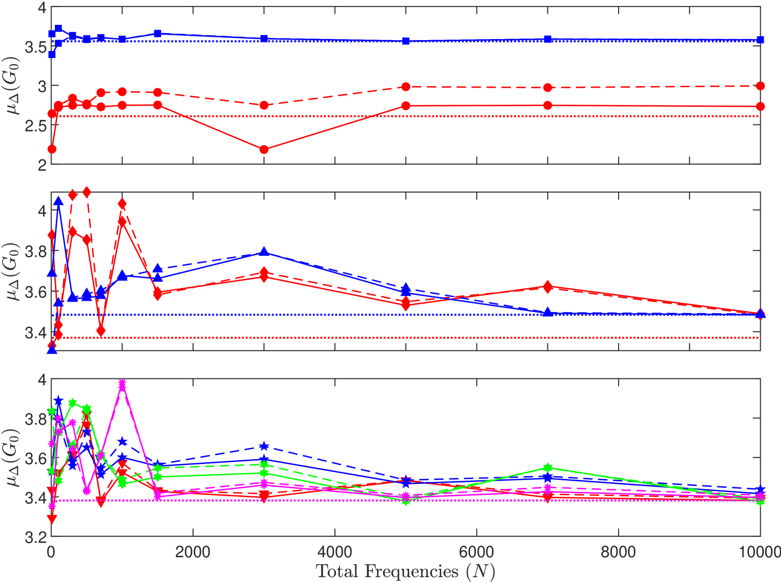
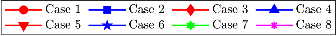
Figure 1: Comparison between $\mu_{\Delta}(G_{0})$ and $N$. Solid line: $\tilde{\mu}$, dashed line: $\bar{\mu}$, dotted line: mussv. From top to bottom, the plots correspond to systems with 1 block, 2 blocks, and 3 blocks, respectively.

Figure 1 presents the results for the configurations described in Table I. Note that, as $N$ increases, the performance of Algorithm 1 improves, as previously discussed. Cases 1 ($f=0$) and 3 ($r_{j}>m_{k}$) do not converge to $\mu_{M}$; this is in agreement with the overall simulation results. Additionally, Cases 2 and 8 exhibit the best convergence across all cases, a result that is both encouraging and of engineering interest, as it suggests that the proposed algorithm is particularly effective in obtaining reliable lower bounds for structured singular value computations in realistic robustness scenarios, where full complex blocks are commonly used to model input-output interactions and coupled perturbations.

In practice, when the number of frequencies $N$ is large, the number of iterations $l$ required for the algorithm to converge typically ranges between 15 and 30. For the test under consideration, where $N=1000$ was used to ensure convergence, Figure 2 illustrates the iterative behavior for cases where the lower bound successfully reaches mussv, highlighting the effect of the number of blocks on the stopping criterion, where a higher number of blocks requires more iterations to meet the termination condition.

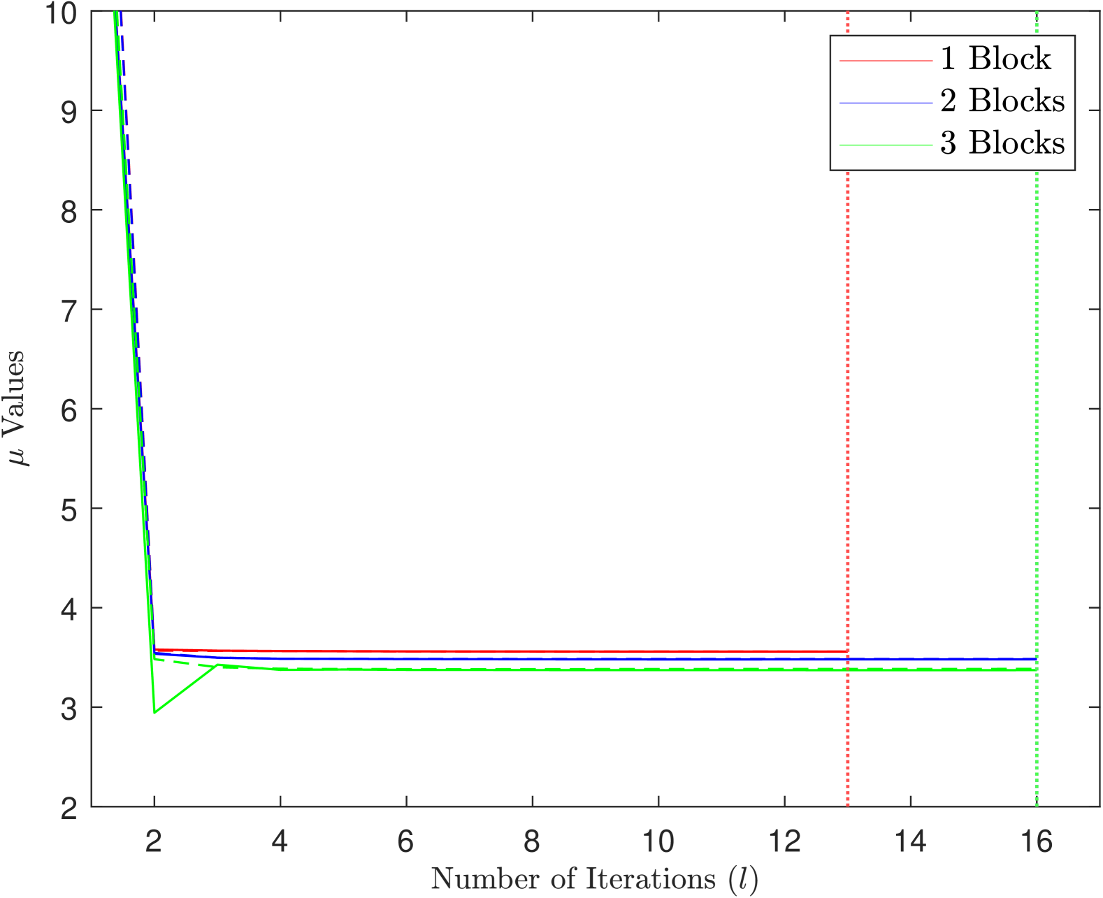
Figure 2: Convergence of the lower bound over iterations $(l)$. Solid line: $\tilde{\mu}$, dashed line: $\bar{\mu}$, dotted line: last iteration.

Figure 3 illustrates the structured singular value as a function of frequency for Case 4. The observed behavior, where $\tilde{\mu}$ and $\bar{\mu}$ align well with mussv at the dominant frequency but deviate at others, is expected based on the properties of the power method [5]. Indeed, the power method generates input signals whose energy iteratively concentrates around the frequency $\omega$ at which the lower bound on $\mu^{\prime}_{\Delta}(\bm{G}_{0}(e^{i\omega}))$ is largest, which leads to better estimates at that frequency at the expense of poorer estimates for other frequencies.

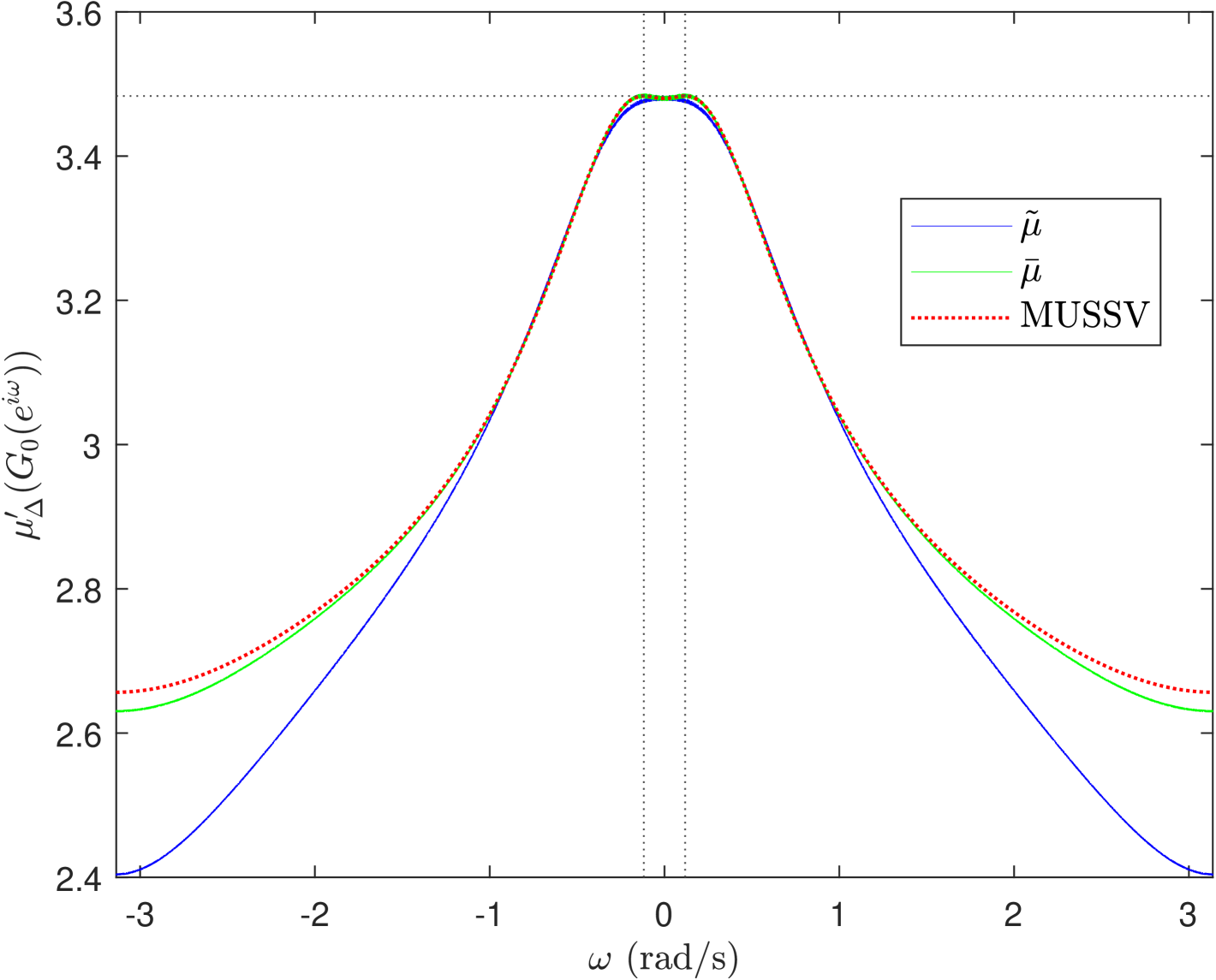
Figure 3: Frequency response of the structured singular value.

TABLE II: Structured singular values, and peak frequencies, for different noise levels.

$\sigma^{2}$	$\tilde{\mu}$		$\bar{\mu}$
	Value	Frequency	Value	Frequency
0	3.4832	0.0000	3.4864	0.1137
$10^{-6}$	3.9034	0.0415	4.1362	0.0258
$10^{-5}$	4.7400	0.1005	6.0842	0.4876
$10^{-4}$	8.2426	2.9016	11.6509	0.3914
$10^{-3}$	22.4976	2.3989	33.6600	0.4115
0.01	65.4947	1.6757	125.8755	2.7307
MUSSV	3.4833	0.1181	–	–

Table II illustrates how Gaussian noise in the output, with variance $\sigma^{2}$, affects the convergence of $\tilde{\mu}$ and $\bar{\mu}$, which show that the algorithm can be sensitive to noise. The algorithm’s robustness to noise can be improved, using, e.g., instrumental variables methods, but this is left for future research.

Test $\#$2

Algorithm 1 has also been tested on a large set of randomly generated matrices. A total of 700 experiments have been conducted for each block structure configuration on $n\times n$ complex matrices, with $n=2,3,\dots,8$, yielding a total of 2100 simulations. The considered block structures are:

• $\bm{r}=[0,0]$ and $\bm{m}=[1,n]$.

• $\bm{r}=[n,1,\cdots,1]$ and $\bm{m}=[0,0]$.

• For even $n$, $\bm{r}=[n/2,1,\dots,1]$ and $\bm{m}=[1,n/2]$. For odd $n$, $\bm{r}=[(n-1)/2,1,\dots,1]$ and $\bm{m}=[1,(n+1)/2]$.

Figure 4 illustrates the percentage of simulations where the average of $\tilde{\mu}$ and $\bar{\mu}$ converge to $\mu_{M}$, which demonstrates better performance for $s=0$ and, across all three cases, a deterioration of the algorithm when $n>5$. It should be noted that, for $s+2f>3$, the exact value of $\mu_{\Delta}(\bm{G}_{0})$ is unknown, potentially introducing bias when comparing the lower bounds to mussv. Nevertheless, the use of randomly generated synthetic matrices provides a first step in evaluating algorithm performance, and future studies could explore its applicability to real-world system dynamics to further assess its robustness.

Overall, the simulations show that Algorithm 1 provides a good estimate of a lower bound on $\mu_{\Delta}(\bm{G}_{0})$, in comparison to $\mu_{M}$. Additionally, we see that our algorithm tends to achieve better convergence in systems with fast dynamics, which could be due to the fact that faster systems have shorter transients contaminating the data.

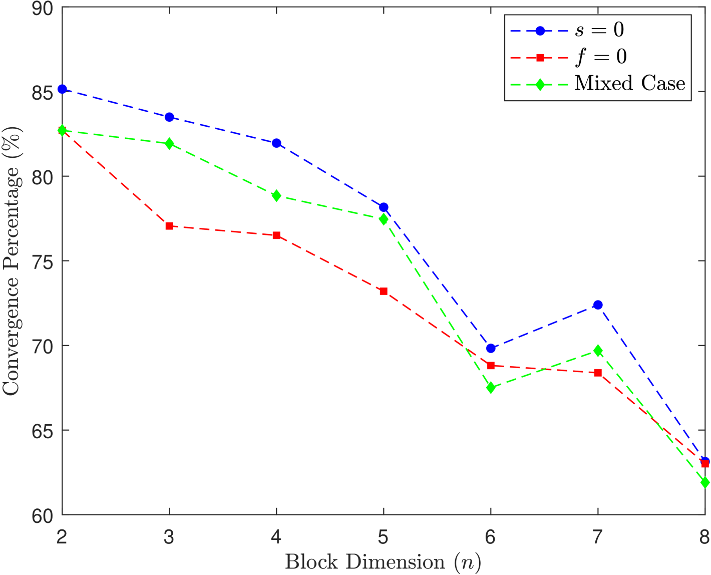
Figure 4: Percentage of converging cases of the data-driven power method.

VI Conclusion

In this paper, we have introduced a data-driven method to estimate a lower bound for the structured singular value of a dynamical system from input-output data. Our approach is model-free, in the sense that a model of the system is not required nor explicitly built. Numerical examples show that our method closely approximates the lower bounds obtained using mussv. For future work, we consider estimating a corresponding upper bound for the structured singular value from input-output data.

References

- [1] L. Ljung, System Identification: Theory for the User, 2nd Edition. Prentice Hall, 1999.
- [2] T. Söderström and P. Stoica, System Identification. Prentice Hall, 1989.
- [3] K. Zhou, J. C. Doyle, and K. Glover, Robust and Optimal Control. Prentice-Hall, 1996.
- [4] B. Wahlberg, M. B. Syberg, and H. Hjalmarsson, “Non-parametric methods for -gain estimation using iterative experiments,” Automatica, vol. 46, no. 8, pp. 1376–1381, 2010.
- [5] C. R. Rojas, T. Oomen, H. Hjalmarsson, and B. Wahlberg, “Analyzing iterations in identification with application to nonparametric -norm estimation,” Automatica, vol. 48, no. 11, pp. 2776–2790, 2012.
- [6] M. I. Müller and C. R. Rojas, “Gain estimation of linear dynamical systems using Thompson sampling,” in Proceedings of the 22nd International Conference on Artificial Intelligence and Statistics (AISTATS), pp. 1535–1543, 2019.
- [7] J. Doyle, “Analysis of feedback systems with structured uncertainties,” IEE Proceedings D (Control Theory and Applications), vol. 129, no. 6, pp. 242–250, 1982.
- [8] V. D. Blondel and J. N. Tsitsiklis, “A survey of computational complexity results in systems and control,” Automatica, vol. 36, no. 9, pp. 1249–1274, 2000.
- [9] A. Packard, M. K. Fan, and J. Doyle, “A power method for the structured singular value,” in Proceedings of the IEEE Conference on Decision and Control, pp. 2132–2137, 1988.
- [10] A. K. Packard, What’s new with mu: Structured uncertainty in multivariable control. PhD thesis, University of California, Berkeley, 1988.
- [11] G. H. Golub and C. F. Van Loan, Matrix Computations. John Hopkins University Press, 2013.
- [12] T. Oomen, R. van der Maas, C. R. Rojas, and H. Hjalmarsson, “Iterative data-driven norm estimation of multivariable systems with application to robust active vibration isolation,” IEEE Transactions on Control Systems Technology, vol. 22, no. 6, pp. 2247–2260, 2014.
- [13] D.-W. Gu, P. H. Petkov, and M. M. Konstantinov, Robust Control Design with MATLAB®. Springer, 2013.