Localized Dynamic Mode Decomposition with Temporally Adaptive Partitioning

Abstract

Dynamic Mode Decomposition (DMD) is a widely used data-driven algorithm for predicting the future states of dynamical systems. However, its standard formulation often struggles with poor long-term predictive accuracy. To address this limitation, we propose a localized DMD framework that improves prediction performance by integrating DMD’s strong short-term forecasting capabilities with time-domain decomposition techniques. Our approach segments the time domain of the dynamical system, independently constructing snapshot matrices and performing localized predictions within each segment. We first introduce a localized DMD method with predefined partitioning, which is simple to implement, and then extend it to an adaptive partitioning strategy that enhances prediction accuracy, robustness, and generalizability. Furthermore, we conduct an error analysis that provides the upper bound of the local and global truncation error for our method. To demonstrate the effectiveness of our approach, we apply it to four benchmark problems: Burgers’ equation, the Allen-Cahn equation, the nonlinear Schrödinger equation, and Maxwell’s equations. Numerical results show that our method significantly improves both predictive accuracy and computational efficiency.

Keywords: dynamic mode decomposition, dynamical systems, temporally adaptive partitioning, localized dynamic mode decomposition

MSCcodes: 37M10, 37M99, 65P99

1 Introduction

Dynamic mode decomposition (DMD) [32] has emerged as a powerful data-driven technique. This method has found extensive applications across diverse domains including physics [7], engineering [9], control [29], and machine learning [26]. The core idea of the DMD method is to approximate a linear mapping of a given time-series data matrix, enabling the data to evolve in a low-dimensional subspace while extracting its main dynamic characteristics.

The DMD method is closely related to the Arnoldi method [33] in analyzing the characteristic patterns and dynamic behaviors of processing systems. The core of the Arnoldi method involves iteratively generating Krylov subspaces and using the orthogonalization process to construct low-dimensional projection matrices. In contrast, DMD employs the Koopman operator theory [27, 30] as a bridge to extract system features and spatio-temporal evolution modes, positioning DMD as an approximation of the Koopman operator in finite-dimensional space [3]. This connection forms a solid foundation for DMD to handle nonlinear systems, making its framework increasingly perfect in theoretical [6, 37] and numerical [1]. Subsequent research established the convergence of the DMD algorithm under the strong operator topology(SOT) [14]. Additionally, the use of the Liouville operator as a replacement for the Koopman operator has been proposed to optimize the analysis of DMD algorithm convergence [31]. Furthermore, the prediction accuracy of DMD has been analyzed through parabolic equations, considering both local and global truncation errors [23].

With the application of DMD in practice, the basic methods are continuously improved to address challenges in practical problems. The DMD method has produced multiple variants [34]: Optimized DMD(OptDMD) [27, 4, 2, 18] methods aimed at reducing the sensitivity of DMD to noise, as well as approaches that integrate DMD with data assimilation techniques such as Kalman filtering [43] or ensemble Kalman filtering [8]. Methods like Extended DMD(EDMD) [39] and Kernel DMD(KDMD) [38, 17] are designed to handle strongly nonlinear systems. In contrast, the Multiresolution DMD(mrDMD) method [16] excels at capturing multi-scale behavior and managing translational or rotational structures that traditional SVD-based methods cannot effectively address. Additionally, the Higher Order DMD(HODMD) [5] method leverages Takens’ delayed embedding theorem [36] to incorporate richer temporal information and historical states.

The time-domain decomposition method is a widely utilized computational strategy in time-parallel algorithms [40, 41, 42] and large time-scale complex systems, particularly in the study of dynamical systems. Several time series segmentation techniques have been proposed, including the Top–Down algorithm, the Bottom–Up algorithm, and the Sliding Window algorithm [22]. The Top–Down algorithm [28] determines breakpoints based on prior knowledge or heuristic approaches. However, it is often criticized for its limited flexibility; The Bottom–Up algorithm [10, 24] ensures high segmentation accuracy by iteratively merging smaller segments into larger ones until a desired structure is obtained; The Sliding Window algorithm [25] incorporates an adaptive, online segmentation mechanism, avoiding redundant computations and significantly enhancing computational efficiency. It is simple to implement, highly flexible, and broadly applicable across diverse scenarios.

Regardless of the specific variant or application of the DMD method, its primary objective remains the accurate identification of spatio-temporal coherent structures in complex systems or the reliable prediction of long-term dynamics. However, standard DMD often struggles with long-term accuracy, and while various extensions have been proposed, they remain limited by specific assumptions or application constraints. Inspired by the time-domain decomposition method [22, 11], which partitions long-time-scale problems into multiple shorter segments, we propose an enhanced approach for modeling time-varying nonlinear dynamical systems. By strategically segmenting the temporal domain, the local linear behavior within each sub-time interval becomes more prominent, enabling DMD to make more reliable predictions within each segment. To achieve this, we develop a localized DMD method, which integrates the Sliding Window algorithm with the data-driven nature of DMD, ensuring computational feasibility and efficiency. Our LDMD operates in a sequential manner, using the previous stage’s final prediction as the initial condition for the next stage. These corrected solutions serve as high-quality snapshots for the current stage, ensuring robust and accurate approximation across the entire time domain. Additionally, we incorporate an adaptive partitioning strategy [12] with an error estimator to adaptively determine the number of time steps for each stage, keeping prediction errors controlled within a stable range. This approach achieves higher accuracy, broader applicability, and faster computation for long-term predictions.

The outline of this paper is as follows: In section 2, we briefly review the DMD method and its connection to Koopman operator theory. In section 3, we introduce our localized DMD with predefined portioning that requires prior knowledge of time segmentation, and localized DMD with adaptive portioning that applies residual equations as error estimators. In section 4, we provide an upper bound of the local and global truncation error of the localized DMD method. In section 5, we selected some representative and important numerical examples to verify that our method achieves smaller errors and faster calculation speed than that of the standard DMD method. In section 6, we summarize the results with a discussion of advantages, challenges, and future work.

2 The DMD

DMD is a widely recognized technique that utilizes system data measurements exclusively to approximate the underlying spatiotemporal dynamics and provide predictions. In this section, we present the general form of the dynamical system as follows:

$$\frac{\partial\mathbf{u}(t,\mathbf{x})}{\partial t}=\mathbf{f}(\mathbf{u},D\mathbf{u},D^{2}\mathbf{u},\cdots),\quad\mathbf{x}\in\Omega\subset\mathbb{R}^{N_{x}},\quad t\in[t_{0},T],$$ (2.1)

where $\mathbf{u}(t,\mathbf{x})$ represents the solution vector at time $t$ and spatial coordinates $\mathbf{x}\in\Omega$, $N_{x}$ denotes the spatial degrees of freedom in the system. The function $\mathbf{f}\in\mathbb{C}^{N_{x}}$ characterizes a linear or nonlinear function involving $\mathbf{u}$ and its spatial derivatives. The initial condition of the system (2.1) is $\mathbf{u}(t_{0},\mathbf{x})=\mathbf{u}_{0}(\mathbf{x})$, while the boundary conditions may be Dirichlet, Neumann, or mixed types.

For (2.1) discretely sampled in time is governed by the discrete-time dynamical system

$$\mathbf{u}_{k+1}=\mathbf{F}(\mathbf{u}_{k}),$$ (2.2)

where $\mathbf{u}_{k}=\mathbf{u}(t_{0}+k\Delta t,\mathbf{x})$ with $\Delta t$ being the size of the time step, $N_{t}$ denotes the time degrees of freedom in the system. $\mathcal{M}$ denotes the state space, and $\mathbf{F}$ is a map from $\mathcal{M}$ to itself. Let $\mathbf{F}^{t}\colon\mathcal{M}\to\mathcal{M}$ be the flow map operator, and $\mathbf{F}^{t-t_{0}}$ advance the initial conditions $\mathbf{u}_{0}(\mathbf{x})$ to the dynamical system (2.1) from initial time $t_{0}$ to final time $t$. Therefore trajectories evolve according to

$$\mathbf{u}(t,\mathbf{x})=\mathbf{F}^{t-t_{0}}(\mathbf{u}_{0}(\mathbf{x})).$$ (2.3)

DMD is deeply connected to the Koopman theory. We briefly review the Koopman operator theory and the DMD algorithm in subsections 2.1 and 2.2.

2.1 Koopman operator and its mode decomposition

The Koopman operator is a linear operator defined in the space of observation functions, which facilitates the representation of nonlinear dynamical systems in the state space as linear systems in the observation function space. For dynamical systems (2.1) or (2.3), the family of Koopman operators parameterized by time variable $t$ can be defined as follows.

Definition 2.1 (The family of Koopman operator).

Let $\bm{G}(\mathcal{M})$ be an infinite dimensional observation function space for any scalar-valued observable function $g:\mathcal{M}\rightarrow\mathbb{C}$. The family of Koopman operator $\mathcal{K}^{t}:\bm{G}(\mathcal{M})\rightarrow\bm{G}(\mathcal{M})$ is defined by

$$\mathcal{K}^{t}g(\mathbf{u}):=g\big{(}\mathbf{F}^{t}(\mathbf{u})\big{)},\quad\forall g\in\bm{G}(\mathcal{M}).$$ (2.4)

Definition 2.2 (Koopman operator [15]).

The discrete-time dynamical system (2.2) also known as a flow map is more general than the continuous-time formulation. The corresponding discrete-time Koopman operator $\mathcal{K}$ is

$$\mathbf{u}_{k+1}=\mathbf{F}(\mathbf{u}_{k})\Rightarrow g(\mathbf{u}_{k+1})=\mathcal{K}g(\mathbf{u}_{k}),$$ (2.5)

where $\mathcal{K}$ is an infinite-dimensional linear operator that acts on the Hilbert space.

The spectral decomposition theory of the Koopman operator can give an expression for the observation functions. Let $(\lambda_{i},\varphi_{i})_{i=1}^{\infty}$ denote the eigenpairs of the Koopman operator $\mathcal{K}$. By performing multiple take multiple measurements of the system, we obtain a set of scalar observation functions $\mathbf{g}=\{g_{1},\ldots,g_{q}\}$. Each observation function can then be represented as a linear combination of the eigenfunctions of the Koopman operator:

$$\left.\left.\left.\mathbf{g}(\mathbf{u})=\left[\begin{array}[]{c}g_{1}(\mathbf{u})\\ \vdots\\ g_{q}(\mathbf{u})\end{array}\right.\right.\right.\right]=\sum_{i=1}^{\infty}\varphi_{i}(\mathbf{u})\begin{bmatrix}<\varphi_{i},g_{1}>\\ \vdots\\ <\varphi_{i},g_{q}>\end{bmatrix}=\sum_{i=1}^{\infty}\varphi_{i}(\mathbf{u})\mathbf{v}_{i},\quad\mathbf{v}_{i}=\begin{bmatrix}<\varphi_{i},g_{1}>\\ \vdots\\ <\varphi_{i},g_{q}>\end{bmatrix}.$$ (2.6)

Based on (2.5) and (2.6), the dynamics of the observable function $\mathbf{g}(\mathbf{\mathbf{u}}_{k})$ can be represented in discrete form as:

$$\mathbf{g}(\mathbf{u}_{k+1})=\sum_{i=1}^{\infty}\lambda_{i}^{k}\varphi_{i}(\mathbf{u}_{0})\mathbf{v}_{i}.$$

The sequence of triples $\{(\lambda_{i},\varphi_{i},\mathbf{v}_{i})\}_{j=1}^{\infty}$ constitutes the Koopman mode decomposition. In this context, the DMD eigenvalues serve as approximations to the Koopman eigenvalues $\lambda_{i}$, the DMD modes approximate the Koopman modes $\mathbf{v}_{i}$, and the amplitudes of the DMD mode approximate the Koopman eigenfunctions evaluated at the initial condition $\varphi_{i}(\mathbf{u}_{0})$. When the chosen observable functions $\mathbf{g}=\{g_{1},\ldots,g_{q}\}$ are constrained to an invariant subspace spanned by the eigenfunctions of the Koopman operator $\mathcal{K}$, they induce a finite-dimensional linear operator [3].

2.2 The DMD algorithm

DMD is an equation-free data-driven method that relies solely on observational data to approximate the Koopman eigenvalues and eigenvectors. Given a sequence of snapshot data $\{\mathbf{y}_{0},\mathbf{y}_{1},\cdots,\mathbf{y}_{M}\}$, sampled at uniform time intervals $\Delta t$, where $\mathbf{y}=\mathbf{g}(\mathbf{u})$ represents the observation function, DMD is used to extract key dynamical features from the dataset.

We define the data matrices of observables $\mathbf{Y}_{1}$ and $\mathbf{Y}_{2}$ as follows:

$$\begin{gathered}\mathbf{Y}_{1}=\begin{bmatrix}|&|&&|\\ \mathbf{y}_{0}&\mathbf{y}_{1}&\cdots&\mathbf{y}_{M-1}\\ |&|&&|\end{bmatrix}=\begin{bmatrix}|&|&&|\\ \mathbf{g}(\mathbf{u}_{0})&\mathbf{g}(\mathbf{u}_{1})&...&\mathbf{g}(\mathbf{u}_{M-1})\\ |&|&&|\end{bmatrix}\in\mathbb{C}^{qN_{x}\times M},\\ \mathbf{Y}_{2}=\begin{bmatrix}|&|&&|\\ \mathbf{y}_{1}&\mathbf{y}_{2}&\cdots&\mathbf{y}_{M}\\ |&|&&|\end{bmatrix}=\begin{bmatrix}|&|&&|\\ \mathbf{g}(\mathbf{u}_{1})&\mathbf{g}(\mathbf{u}_{2})&...&\mathbf{g}(\mathbf{u}_{M})\\ |&|&&|\end{bmatrix}\in\mathbb{C}^{qN_{x}\times M},\end{gathered}$$ (2.7)

where $M$ is the number of snapshots. The objective of DMD is to determine a matrix $\mathbf{A}\in\mathbb{C}^{qN_{x}\times qN_{x}}$ that satisfies

$$\mathbf{Y}_{2}=\mathbf{A}\mathbf{Y}_{1},$$

where $\mathbf{A}$ serves as an approximation of the finite-dimensional Koopman operator $\mathbf{K}$. The best-fit DMD matrix is obtained by solving the following optimization problem:

$$\mathbf{A}=\underset{\mathbf{A}\in\mathbb{C}^{qN_{x}\times qN_{x}}}{\arg\min}\left\|\mathbf{Y}_{2}-\mathbf{A}\mathbf{Y}_{1}\right\|_{F}=\mathbf{Y}_{2}\mathbf{Y}_{1}^{\dagger},$$

where $\|\cdot\|_{F}$ represents the Frobenius norm, and $\dagger$ denotes the Moore-Penrose pseudo-inverse. The DMD algorithm approximates the eigenvalues and eigenvectors of $\mathbf{A}$ in the observable space. It is very expensive to do eigendecomposition directly on the matrix $\mathbf{A}$. In practical computations, we employ Algorithm 1 to approximate the eigenvalues and eigenvectors of $\mathbf{A}$ efficiently.

Algorithm 1 Standard DMD

0: Snapshots $\{\mathbf{y}_{0},\mathbf{y}_{1},\dots,\mathbf{y}_{M}\}$, truncated rank $r$

0: DMD solution $\mathbf{u}^{\text{DMD}}(t,\mathbf{x})$

1: Construct $\mathbf{Y}_{1}$ and $\mathbf{Y}_{2}$ as defined in (2.7).

2: Perform singular value decomposition (SVD) on $\mathbf{Y}_{1}$: $\mathbf{Y}_{1}\approx\mathbf{U}\mathbf{\Sigma}\mathbf{V}^{H}$ with $\mathbf{U}\in\mathbb{C}^{N_{x}\times r},\mathbf{\Sigma}\in\mathbb{C}^{r\times r},\mathbf{V}\in\mathbb{C}^{M\times r}.$

3: Define the reduced-order operator: $\tilde{\mathbf{A}}=\mathbf{U}^{H}\mathbf{Y}_{2}\mathbf{V}\mathbf{\Sigma}^{-1}.$

4: Compute the eigenvalues and eigenvectors of $\tilde{\mathbf{A}}$:$\tilde{\mathbf{A}}\mathbf{W}=\mathbf{W}\mathbf{\Lambda},\quad\mathbf{\Lambda}=\text{diag}(\lambda_{i}).$

5: Compute the DMD modes: $\mathbf{\Phi}=\mathbf{U}\mathbf{W}.$

6: Compute the future state in the observable space: $\mathbf{g}^{\text{DMD}}(\mathbf{u}_{k})=\mathbf{\Phi}\mathbf{\Lambda}^{k}\mathbf{b}$ with $\mathbf{b}=\mathbf{\Phi}^{\dagger}\mathbf{g}(\mathbf{u}_{0}),$ and its continuous formulation: $\mathbf{g}^{\text{DMD}}(\mathbf{u}(t,\mathbf{x}))=\mathbf{\Phi}\,\text{diag}(\exp(\omega t))\mathbf{b}$ with $\omega_{i}=\frac{\ln(\lambda_{i})}{\Delta t}.$

7: Transform back to the state space: $\mathbf{u}^{\text{DMD}}(t,\mathbf{x})=\mathbf{g}^{-1}(\mathbf{g}^{\text{DMD}}(\mathbf{u}(t,\mathbf{x}))),$ where $\mathbf{g}^{-1}$ is determined in the least-squares sense if $\mathbf{g}$ is not invertible.

Remark 2.1.

Within the framework of Koopman theory, selecting an appropriate observation function is essential for improving the predictive accuracy of the DMD method. However, this process typically requires specialized knowledge and a thorough understanding of the underlying dynamical system.

For systems exhibiting strong nonlinearities or oscillatory behavior, the modes extracted by DMD may fail to accurately capture the system’s intrinsic dynamics, leading to reduced predictive performance. In the subsequent section, we propose a localized DMD approach, which employs a proper temporal partitioning strategy to enhance the predictive accuracy of the DMD method.

3 Localized DMD Method

In the simulation of time-dependent physical systems, the computational domain often comprises multiple subdomains with distinct physical properties, leading to significantly varying characteristic time scales. Inspired by time-domain decomposition principles, this study introduces a segmentation strategy for the temporal domain, optimizing the application of the DMD method to extract essential features from distinct temporal phases.

Time-domain decomposition method partitions a given time interval $[t_{0},t_{N}]$ into multiple sub-intervals, such as $[t_{0},t_{1}],\dots,[t_{N-1},t_{N}]$, where sub-interval lengths may be uniform or variable. It significantly improves computational efficiency while addressing the challenges associated with solving complex dynamical systems over long time horizons.

3.1 Localized DMD with Predefined Partitioning

The Localized DMD (LDMD) method integrates the remarkable short-term predictive ability of DMD with time-domain decomposition techniques. By partitioning extended temporal domains into discrete intervals, LDMD enhances accuracy and robustness in predictive modeling, particularly in complex dynamical systems where conventional approaches often struggle. This method preserves the system’s intrinsic dynamics while adapting to temporal variations, ensuring optimal performance across different time scales.

To implement this approach, the time domain $[t_{0},T]$ is divided into $N$ sub-intervals based on prior knowledge of the system (2.1):

$$t_{0}<t_{1}<\dots<t_{N}=T,$$

where each sub-interval is referred to as a stage. Within each stage, the initial segment of the data is utilized to construct the snapshot matrix, which is subsequently leveraged to predict the remaining portion. Let $\hat{\mathbf{Y}}^{i}_{1}$ and $\hat{\mathbf{Y}}^{i}_{2}$ denote the snapshot matrices for the $i$-th stage, where $i=1,2,\dots,N$, as defined in (2.7). Supposing $n_{i}$ columns are selected as the snapshot matrices in each stage, then $\hat{\mathbf{Y}}^{i}_{1}$ and $\hat{\mathbf{Y}}^{i}_{2}$ are constructed as follows:

$$\begin{gathered}\hat{\mathbf{Y}}_{1}^{i}=\begin{bmatrix}|&|&&|\\ \mathbf{y}^{i}_{0}&\mathbf{y}^{i}_{1}&\dots&\mathbf{y}^{i}_{n_{i}-1}\\ |&|&&|\end{bmatrix}=\begin{bmatrix}|&|&&|\\ \mathbf{g}(\mathbf{u}^{i}_{0})&\mathbf{g}(\mathbf{u}^{i}_{1})&\dots&\mathbf{g}(\mathbf{u}^{i}_{n_{i}-1})\\ |&|&&|\end{bmatrix}\in\mathbb{C}^{qN_{x}\times n_{i}},\\ \hat{\mathbf{Y}}_{2}^{i}=\begin{bmatrix}|&|&&|\\ \mathbf{y}^{i}_{1}&\mathbf{y}^{i}_{2}&\dots&\mathbf{y}^{i}_{n_{i}}\\ |&|&&|\end{bmatrix}=\begin{bmatrix}|&|&&|\\ \mathbf{g}(\mathbf{u}^{i}_{1})&\mathbf{g}(\mathbf{u}^{i}_{2})&\dots&\mathbf{g}(\mathbf{u}^{i}_{n_{i}})\\ |&|&&|\end{bmatrix}\in\mathbb{C}^{qN_{x}\times n_{i}},\end{gathered}$$ (3.1)

where $\mathbf{u}_{k}^{i}$ represents the state vector for the $i$-th stage, and $\mathbf{y}_{k}^{i}$ represents the observation vector for the $i$-th stage. For stage $i=1$, $\{\mathbf{y}_{0}^{1},\mathbf{y}_{1}^{1},\dots,\mathbf{y}_{n_{1}}^{1}\}=\{\mathbf{y}_{0},\mathbf{y}_{1},\dots,\mathbf{y}_{n_{1}}\}$. For stages $i\geq 2$, the final state of the previous stage is used as the initial condition for the subsequent stage. With this initialization, we employ a full-order method (FOM)—such as the finite difference method (FDM) or finite element method (FEM)—to generate snapshot data within each stage. The governing equation for the FOM is given by:

$$\frac{\partial\mathbf{u}^{i}(t,\mathbf{x})}{\partial t}=\mathbf{f}(\mathbf{u}^{i},D\mathbf{u}^{i},D^{2}\mathbf{u}^{i},\dots),\quad\mathbf{x}\in\Omega\subset\mathbb{R}^{N_{x}},\quad t\in[t_{i-1},t_{(i-1)^{\prime}}],$$ (3.2)

where $t_{(i-1)^{\prime}}=t_{i-1}+n_{i}\times\Delta t$ for $i=2,3,\dots,N$, and the initial condition is set as $\mathbf{u}(t_{i-1},\mathbf{x})=\mathbf{u}^{\text{LDMD}}(t_{i-1},\mathbf{x})$.

By ensuring the accuracy of the selected snapshot data at each stage, this method effectively mitigates error accumulation caused by noise, thereby maintaining the reliability of the extracted features. Additionally, by strategically controlling predicted time steps per stage, it achieves higher prediction accuracy even using fewer total snapshots compared to the standard DMD. The main steps of our LDMD are summarized in Algorithm 2.

Algorithm 2 LDMD with Predefined Partitioning

0: Given the number of stages $N$, snapshots $\{\mathbf{y}_{0},\mathbf{y}_{1},\dots,\mathbf{y}_{n_{1}}\}$, and the truncated rank $r$.

0: The solution of LDMD with predefined partitioning $\{\mathbf{u}^{\text{LDMD},i}(t,\mathbf{x})\}_{i=1}^{N}$.

1: for $i=1,2,\dots,N-1$ do

2:  Construct the DMD model with snapshots $\{\mathbf{y}^{i}_{0},\mathbf{y}^{i}_{1},\dots,\mathbf{y}^{i}_{n_{i}}\}$.

3:  Predict $\mathbf{u}^{\text{LDMD},i}(t,\mathbf{x})$ at time interval $[t_{i-1},t_{i}]$.

4:  Compute the FOM as the initial value $\mathbf{u}^{\text{LDMD},i}(t_{i},\mathbf{x})$ at time interval $[t_{i},t_{i^{{}^{\prime}}}]$ to get the snapshots with $n_{i+1}$ columns.

5: end for

6: Construct the DMD model with snapshots $\{\mathbf{y}^{N}_{0},\mathbf{y}^{N}_{1},\dots,\mathbf{y}^{N}_{n_{N}}\}$.

7: Predict $\mathbf{u}^{\text{LDMD},N}(t,\mathbf{x})$ at time interval $[t_{N-1},t_{N}]$.

It is worth noting that merely reducing the number of prediction time steps in each stage does not necessarily increase the accuracy of the snapshot data computed by the FOM in the next stage. Therefore, the appropriate temporal segmentation method is crucial.

3.2 Localized DMD with Adaptive Partitioning

In this section, we propose an adaptive partitioning method to further enhance the generalizability of the proposed LDMD approach without requiring a detailed understanding of the underlying dynamical system.

For LDMD with adaptive partitioning, it is essential to establish precise criteria for determining when to terminate predictions after each application of the DMD algorithm. Unlike predefined partitioning methods, the core idea of adaptive partitioning is to use an error estimator $\Delta_{k}$ [13] to evaluate the prediction accuracy and a tolerance threshold $\epsilon$ to control the prediction error. When $\Delta_{k}$ exceeds $\epsilon$, the FOM is invoked to correct the prediction, reducing the error estimator $\Delta_{k}$. Since the reference solution of the underlying system (2.1) is unavailable, we employ an error estimator $\Delta_{k}$ to evaluate the prediction accuracy. Given that $\Delta_{k}$ is bounded by $\epsilon$, and assuming our LDMD predicts $m_{i}$ steps in each stage. We define the prediction rate $\gamma$ as the ratio of the prediction time step to the total time steps, i.e., $\gamma=\frac{M}{N_{t}}$ for standard DMD method, and

$$\gamma=\frac{\sum_{i=1}^{N}m_{i}}{N_{t}},$$ (3.3)

for LDMD with adaptive partitioning. The prediction rate $\gamma$ generally decreases as $\epsilon$ becomes smaller, indicating a functional dependence on the error threshold $\epsilon$.

To determine the optimal prediction steps $m_{i}$ at each stage $i$, directly computing the error estimator $\Delta_{k}$ at every prediction node is impractical due to its high computational cost. Instead, we evaluate $\Delta_{k}$ just at some given steps $m$ and compare it to a predefined upper bound. If the bound is exceeded, the prediction for the current stage stops, and the next stage begins. In the new stage $i+1$, we use FOM to compute $n_{i+1}$ steps and form the snapshot matrices $\hat{\mathbf{Y}}^{i+1}_{1}$ and $\hat{\mathbf{Y}}^{i+1}_{2}$. To guide this process, error evaluation is primarily based on residual equations, which serve as the key criterion in our approach in this work.

3.3 Evaluation Criteria Based on Residuals

The residual is an effective measure of the deviation between the approximate solution and the reference solution. It provides an accurate assessment of prediction accuracy without requiring direct access to the reference solution, making it a practical and reliable indicator for error evaluation.

Using the explicit method, we discretize the equation (2.1) as:

$$\frac{\mathbf{u}(t_{k+1},\mathbf{x})-\mathbf{u}(t_{k},\mathbf{x})}{\Delta t}=\mathbf{f}(\mathbf{u}(t_{k},\mathbf{x}),D\mathbf{u}(t_{k},\mathbf{x}),\dots).$$ (3.4)

Defining $\mathbf{u}(t_{k},\mathbf{x})=\mathbf{u}_{k}$, $\mathbf{u}(t_{k+1},\mathbf{x})=\mathbf{u}_{k+1}$, and $\mathbf{f}(\mathbf{u}(t_{n},\mathbf{x}),D\mathbf{u}(t_{k},\mathbf{x}),\dots)=\mathbf{f}_{k}$, we substitute the predicted solution $\mathbf{u}^{\text{LDMD}}$ into equation (3.4) to derive the residual equation:

$$\mathbf{R}_{k}=\frac{\mathbf{u}_{k+1}^{\text{LDMD}}-\mathbf{u}_{k}^{\text{LDMD}}}{\Delta t}-\mathbf{f}_{k}.$$ (3.5)

Equation (3.5) shows that the residual reflects prediction accuracy. A zero residual indicates that the predicted results are completely consistent with the dynamical system, whereas a large residual indicates significant deviation, necessitating further correction. Consequently, the residual equation provides a reliable error estimator, which can be defined as the norm of the residual:

$$\Delta_{k}=\|\mathbf{R}_{k}\|_{F}=\|\frac{\mathbf{u}_{k+1}^{\text{LDMD}}-\mathbf{u}_{k}^{\text{LDMD}}}{\Delta t}-\mathbf{f}_{k}\|_{F},$$

where $\|\cdot\|_{F}$ denotes the Frobenius norm. Based on this foundation, we now outline the main steps in Algorithm 3.

Remark 3.1.

Data assimilation methods, such as Kalman filters or ensemble Kalman filters, can also serve as error estimators by computing the error covariance matrix of the state vector. In the future, we will focus on data-driven approaches, including machine learning and data assimilation, as alternative error estimation methods that do not rely on explicit access to governing equations, thereby enhancing applicability to complex or partially known dynamical systems.

Algorithm 3 LDMD with Adaptive Partitioning

0: Given the size of the time window $m$, snapshots $\{\mathbf{y}_{0},\mathbf{y}_{1},\dots,\mathbf{y}_{n_{1}}\}$, the truncated rank $r$, and the residual allowable upper bound $\epsilon$.

0: The solution of LDMD with adaptive partitioning $\{\mathbf{u}^{\text{LDMD},i}(t,\mathbf{x})\}_{i=1}^{N}$.

1: Set the stage counter $c_{i}=0$ with the stage $i=1$ and the residual $\Delta_{k}=0$.  

2: while $\sum_{i}n_{i}+\sum_{i}c_{i}\times m<N_{t}$ do

3:  while $\Delta_{k}<\epsilon$ and $\sum_{i}n_{i}+\sum_{i}c_{i}\times m<N_{t}$ do

4:   Construct the DMD model with snapshots $\{\mathbf{y}^{i}_{0},\mathbf{y}^{i}_{1},\dots,\mathbf{y}^{i}_{n_{i}}\}$.

5:   Advance the prediction time step $m$ and calculate the residual $\Delta_{k}$ here.

6:   $c_{i}=c_{i}+1$.

7:  end while

8:  Compute the FOM as the initial value $\mathbf{u}^{\text{LDMD},i}(t_{i},\mathbf{x})$ to get the snapshots with $n_{i+1}$ columns.

9:  $i=i+1$.

10:  Set the stage counter $c_{i}=0$.

11: end while

12: $N=i$.

Remark 3.2.

In the algorithm 3, the truncated rank $r$ can also be selected adaptively. A common approach is to sort the indices based on the squared singular values in descending order, i.e.,

$$\sigma_{1}^{2}>\sigma_{2}^{2}>\cdots>\sigma_{d}^{2},$$

and determine the truncated rank $r$ such that the following condition is satisfied:

$$\frac{\sum_{j=1}^{r}\sigma^{2}_{j}}{\sum_{j=1}^{d}\sigma^{2}_{j}}\geq 1-\eta,$$

where $\sigma_{j}$ are the singular values of the snapshot matrix $\hat{\mathbf{Y}}_{1}^{i}$ and $d$ denotes the rank of the snapshot matrix $\hat{\mathbf{Y}}_{1}^{i}$. The parameter $\eta$ is a threshold for rank selection, typically chosen as $10^{-8}$ or $10^{-10}$.

4 Error analysis

In this section, we conduct a theoretical error analysis based on the FOM solution to demonstrate that our LDMD provides an upper bound for both local and global truncation errors.

Selecting appropriate observations for different equations is often challenging, as it requires a comprehensive understanding of the system. Our LDMD method addresses this issue by decomposing complex dynamical systems with large time scales into multiple smaller time-scale segments, effectively reducing the system’s nonlinear behavior within each segment. Consequently, accurate predictions can be achieved by applying identity observations $g(\mathbf{u})=\mathbf{u}$. The linearized discrete-time approximation of system (2.1) is given by

$$\mathbf{u}_{k+1}=\mathbf{K}\mathbf{u}_{k},\quad k=0,1,\cdots,N_{t}$$ (4.1)

where

$$\mathbf{K}=\underset{\mathbf{A}\in\mathbb{C}^{qN_{x}\times qN_{x}}}{\operatorname*{\mathrm{argmin}}}\sum_{k=0}^{N_{t}}\|\mathbf{A}\mathbf{u}_{k}-\mathbf{u}_{k+1}\|_{F}.$$ (4.2)

If the spectral radius of $\mathbf{K}$, denoted as $\rho(\mathbf{K})$, satisfies $\rho(\mathbf{K})<1$, then the following lemma holds:

Lemma 4.1 ([23]).

For the dynamical system (2.1), subsequent DMD prediction results remain bounded by the initial values:

$$||\mathbf{u}_{k+1}||^{2}_{2}<||\mathbf{u}_{0}||^{2}_{2}.$$ (4.3)

Compared with Lemma $3.1$ in [23], our formulation incorporates the source term in (2.1), ensuring that subsequent prediction results remain constrained by the initial values, as expressed in (4.3).

Lemma 4.2 ([23]).

Define the local truncation error

$$\mathbf{\tau}^{\text{DMD}}_{k}=\mathbf{u}_{k}-\mathbf{u}^{\text{DMD}}_{k}(\mathbf{u}_{k-1}).$$

Then, for any $k\geq M$,

$$||\mathbf{\tau}^{\text{DMD}}_{k}||^{2}_{2}\leq\varepsilon_{M},$$

where $\varepsilon_{M}$ is a constant dependent only on the number of snapshots $M$.

From Lemma 4.1 and Lemma 4.2, we can deduce the local truncation error bound of our LDMD method.

Theorem 4.1.

Define the local truncation error of the LDMD with adaptive partitioning

$$\mathbf{\tau}^{\text{LDMD}}_{k}=\mathbf{u}_{k}-\mathbf{u}^{\text{LDMD}}_{k}(\mathbf{u}_{k-1}).$$

Then, for any $k\in[\sum_{j=1}^{i}n_{j}+\sum^{i-1}_{j=0}c_{j}\times m+1,\sum_{j=1}^{i}n_{j}+\sum^{i}_{j=0}c_{j}\times m]$ with $c_{0}=0$,

$$||\mathbf{\tau}^{\text{LDMD}}_{k}||^{2}_{2}\leq\max_{i}\{\varepsilon_{n_{i}}^{i}\},\quad i=1,2,\cdots,N$$

where the superscript $i$ denotes the stage index, and the constant $\varepsilon_{n_{i}}^{i}$ is a constant depending only on the number of snapshots $n_{i}$ at each stage.

Proof.

Since LDMD with adaptive partitioning performs an independent DMD algorithm at each stage, we generate the different Koopman matrix $\mathbf{K}_{i}$ for each stage. Therefore, according to Lemma 4.2 we have the local truncation error

$$||\mathbf{\tau}^{i}_{k}||^{2}_{2}\leq\varepsilon_{n_{i}}^{i},\quad k\in[\sum_{j=1}^{i}n_{j}+\sum^{i-1}_{j=1}c_{j}\times m+1,\sum_{j=1}^{i}n_{j}+\sum^{i}_{j=1}c_{j}\times m].$$

According to the proof of the Lemma 4.2 and the proof of the Theorem 3.3 in [23], we have

$$\varepsilon_{n_{i}}^{i}=||C_{n_{i}}^{i}||^{2}_{2}||\mathbf{u}_{0}||_{2},$$

where $||C_{n_{i}}^{i}||_{2}^{2}$ is the upper bound of

$$(1+\delta)\left\|\underset{\mathbf{A}\in\mathbb{C}^{qN_{x}\times qN_{x}}}{\operatorname*{\mathrm{argmin}}}\sum_{k=0}^{n_{i}+c_{i}\times m-1}||\mathbf{A}\mathbf{u}_{k}-\mathbf{u}_{k+1}||_{2}^{2}-\underset{\mathbf{A}\in\mathbb{C}^{qN_{x}\times qN_{x}}}{\operatorname*{\mathrm{argmin}}}\sum_{k=0}^{n_{i}-1}||\mathbf{A}\mathbf{u}_{k}-\mathbf{u}_{k+1}||_{2}^{2}\right\|^{2}_{2},$$

where $\delta$ is a constant such that $0<\delta\ll 1$.

Thus, the local truncation error bound for LDMD with adaptive partitioning is determined by the maximum error bound over all stages:

$$||\mathbf{\tau}^{\text{LDMD}}_{k}||^{2}_{2}=\max_{i}\{||\tau^{i}_{k}||_{2}^{2}\}\leq\max_{i}\{\varepsilon_{n_{i}}^{i}\},$$

$$k\in[\sum_{j=1}^{i}n_{j}+\sum^{i-1}_{j=0}c_{j}\times m+1,\sum_{j=1}^{i}n_{j}+\sum^{i}_{j=0}c_{j}\times m].$$

∎

In short time intervals, the nonlinearity of complex systems is relatively weak. According to Koopman operator theory, the DMD algorithm can more effectively extract feature information from the system dynamics described by (2.1) for short-term predictions. As a result, the Koopman matrix provides a more precise representation of the system’s dynamics over short time scales, leading to tighter error bounds in the local truncation error. Thus, we can reasonably deduce

$$\max_{i}\{\varepsilon_{n_{i}}^{i}\}<\varepsilon_{M},$$

and

$$||\mathbf{\tau}^{\text{LDMD}}_{k}||^{2}_{2}<||\mathbf{\tau}^{\text{DMD}}_{k}||^{2}_{2}.$$

Lemma 4.3 ([23]).

Define the global truncation error

$$\mathbf{e}^{\text{DMD}}_{k}=\mathbf{u}_{k}-\mathbf{u}^{\text{DMD}}_{k}.$$

Then, for any $k\geq M$,

$$||\mathbf{e}^{\text{DMD}}_{k}||_{2}<||\mathbf{\Phi}||_{2}||\mathbf{\Phi}^{-1}||_{2}[||\mathbf{e}_{M}||_{2}+(k-M)\varepsilon_{M}],$$ (4.4)

where $||\mathbf{e}_{M}||_{2}$ is fixed and minimal [32].

Lemma 4.4.

If the dynamical system (2.1) is stable and well-posed, then the solution depends continuously on the initial conditions, i.e.,

$$||\mathbf{u}(t,\mathbf{x})-\mathbf{w}(t,\mathbf{x})||_{2}\leq L||\mathbf{u}_{0}(\mathbf{x})-\mathbf{w}_{0}(\mathbf{x})||_{2},\quad\forall t\in[t_{0},T],$$ (4.5)

where $\mathbf{u}(t,\mathbf{x}),\mathbf{w}(t,\mathbf{x})$ are solutions of (2.1) corresponding to different initial conditions $\mathbf{u}_{0}(\mathbf{x})$, $\mathbf{w}_{0}(\mathbf{x})$, respectively, and $L$ is a constant.

From Lemma 4.3 and Lemma 4.4, we can deduce the global truncation error bound of our LDMD method.

Theorem 4.2.

Define the global truncation error of the LDMD with adaptive partitioning as

$$\mathbf{e}^{\text{LDMD}}_{k}=\mathbf{u}_{k}-\mathbf{u}^{\text{LDMD}}_{k}.$$

Then, for any $k\in[\sum_{j=1}^{i}n_{j}+\sum^{i-1}_{j=0}c_{j}\times m+1,\sum_{j=1}^{i}n_{j}+\sum^{i}_{j=0}c_{j}\times m]$ with $c_{0}=0$, the following upper bound holds:

$$||\mathbf{e}^{\text{LDMD},i}_{k}||_{2}<\sum_{p=1}^{i}L^{i-p}||\mathbf{\Phi}_{p}||_{2}||\mathbf{\Phi}_{p}^{-1}||_{2}(||\mathbf{e}^{p}_{n_{p}}||_{2}+k^{p}\varepsilon_{n_{p}}^{p}),$$

where $||\mathbf{e}_{n_{i}}^{i}||_{2}$ and $||\mathbf{e}_{n_{p}}^{p}||_{2}$ are fixed and minimal, $k^{p}$ represents the number of predicted time steps in the $p$-th stage.

Proof.

The global truncation error of the LDMD with adaptive partitioning consists of two components:

• The DMD prediction error at the current stage, which follows the error bound described in Lemma 4.3.

• The error propagation from previous stages, due to the reliance on previous stage predictions as initial values.

To formalize the error propagation, we define the accumulated error from the previous stage as:

$$||\mathbf{e}^{\text{LDMD},i-1}_{k}||_{2}:=||\mathbf{E}^{\text{LDMD},i-1}||_{2},$$

where $\mathbf{E}^{\text{LDMD},i-1}$ represents the LDMD prediction error at the end of stage $i-1$, serving as the initial condition for stage $i$.

Applying Lemma 4.3 and Lemma 4.4, we establish the following bound for the global truncation error at stage $i$:

$$||\mathbf{e}^{\text{LDMD},i}_{k}||_{2}<||\mathbf{\Phi}_{i}||_{2}||\mathbf{\Phi}_{i}^{-1}||_{2}(||\mathbf{e}_{n_{i}}^{i}||_{2}+k^{i}\varepsilon_{n_{i}}^{i})+L||\mathbf{E}^{\text{LDMD},i-1}||_{2},$$ (4.6)

where

$$k^{i}=(k-\sum_{j=1}^{i}n_{j}-\sum^{i-1}_{j=0}c_{j}\times m),\quad k\in[\sum_{j=1}^{i}n_{j}+\sum^{i-1}_{j=0}c_{j}\times m+1,\sum_{j=1}^{i}n_{j}+\sum^{i}_{j=0}c_{j}\times m].$$

Here, $||\mathbf{e}_{n_{i}}^{i}||$ represents the error in the DMD reconstruction stage, which is fixed and minimal. $\mathbf{\Phi}_{i}$ represents the mode approximation of the Koopman matrix $\mathbf{K}_{i}$. Additionally, the initial error is zero in the first stage, i.e. $||\mathbf{E}^{\text{LDMD},0}||_{2}=0$.

Performing the recursion in (4.6) iteratively from $i=1$ to $i=N$, we obtain

$$||\mathbf{e}^{\text{LDMD},i}_{k}||_{2}<\sum_{p=1}^{i}L^{i-p}||\mathbf{\Phi}_{p}||_{2}||\mathbf{\Phi}_{p}^{-1}||_{2}(||\mathbf{e}^{p}_{n_{p}}||_{2}+k^{p}\varepsilon_{n_{p}}^{p}),$$

where $k^{p}=c_{p}\times m$ with $p=1,2,\cdots,i-1$. This completes the proof. ∎

5 Numerical results

In this section, we perform four numerical experiments on complex systems, including both linear and nonlinear equations. Under the identical observable function, SVD truncation, and prediction rate, we exhibit that our LDMD method achieves better results and cheaper computational cost than the standard DMD method. As noted in Remark 2.1, selecting proper observable functions requires domain-specific expertise. However, in the absence of such prior knowledge(i.e. the observable is defined as the identity mapping $g(\mathbf{u})=\mathbf{u}$ or choosing observation function at will), our LDMD method still outperforms the standard DMD across all time steps when we have chosen an appropriate time segmentation method or time window size.

In the algorithm implementation process, $n_{i}=m(i\geq 2)$ can be simplified for convenience. The $L^{2}$ relative error measures the reconstruction and prediction accuracy of (L)DMD:

$$RE=\frac{||\mathbf{u}^{\text{(L)DMD}}_{k}-\mathbf{u}^{\text{ref}}_{k}||_{2}}{||\mathbf{u}^{\text{ref}}_{k}||_{2}},$$

where $u^{\text{ref}}_{k}$ represents the reference solution at time $t_{0}+k\Delta t$, for convenience, we refer to the $L^{2}$ relative error as $RE$. The mean $L^{2}$ relative error:

$$MRE=\frac{\sum_{k=1}^{N_{t}}RE}{N_{t}},$$

we refer to the mean $L^{2}$ relative error as $MRE$.

5.1 Burgers’ equation

We begin with the one-dimensional Burgers’ equation with Dirichlet boundary conditions, a nonlinear equation used to describe shock wave and turbulence phenomena. The following equation can describe it,

$$\begin{cases}{\frac{\partial\mathbf{u}}{\partial t}+\mathbf{u}\frac{\partial\mathbf{u}}{\partial x}=\mu\frac{\partial^{2}\mathbf{u}}{\partial x^{2}}},\quad\mathbf{x}\in[-L,L],\quad t\in[0,T],\\ \mathbf{u}(0,\mathbf{x})=-\sin(\pi\mathbf{x}),\\ \mathbf{u}(t,-L)=\mathbf{u}(t,L)=0,\end{cases}$$ (5.1)

where $L=1$, $T=1$ and the viscosity coefficient $\mu=0.01$. The DMD method often needs appropriate observables to capture the eigenvalues and eigenfunctions of the Koopman operator. However, we only select the identity mapping $g(\mathbf{u})=\mathbf{u}$ to demonstrate the powerful predictive stability of our method. We set the spatial domain discretized into $N_{x}=500$ intervals, and the time domain discretized into $N_{t}=2000$ steps. Then, we set

$$r=20,\quad\epsilon=5\times 10^{-5},\quad n_{1}=300,\quad m=50.$$

So the prediction rate $\gamma=50\%$, correspondingly $M=1000$ in the standard DMD method.

To verify the impact of the prediction rate on prediction performance, we consider comparing the prediction performance of LDMD with adaptive partitioning and the standard DMD method at different prediction rates. In one case, we set

$$r=15,\quad\epsilon=10^{-3},\quad n_{1}=200,\quad m=50.$$

So the prediction rate $\gamma=60\%$, correspondingly $M=800$ in the standard DMD method. In another case, we set

$$r=20,\quad\epsilon=10^{-4},\quad n_{1}=400,\quad m=100.$$

So the prediction rate $\gamma=40\%$, correspondingly $M=1200$ in the standard DMD method.

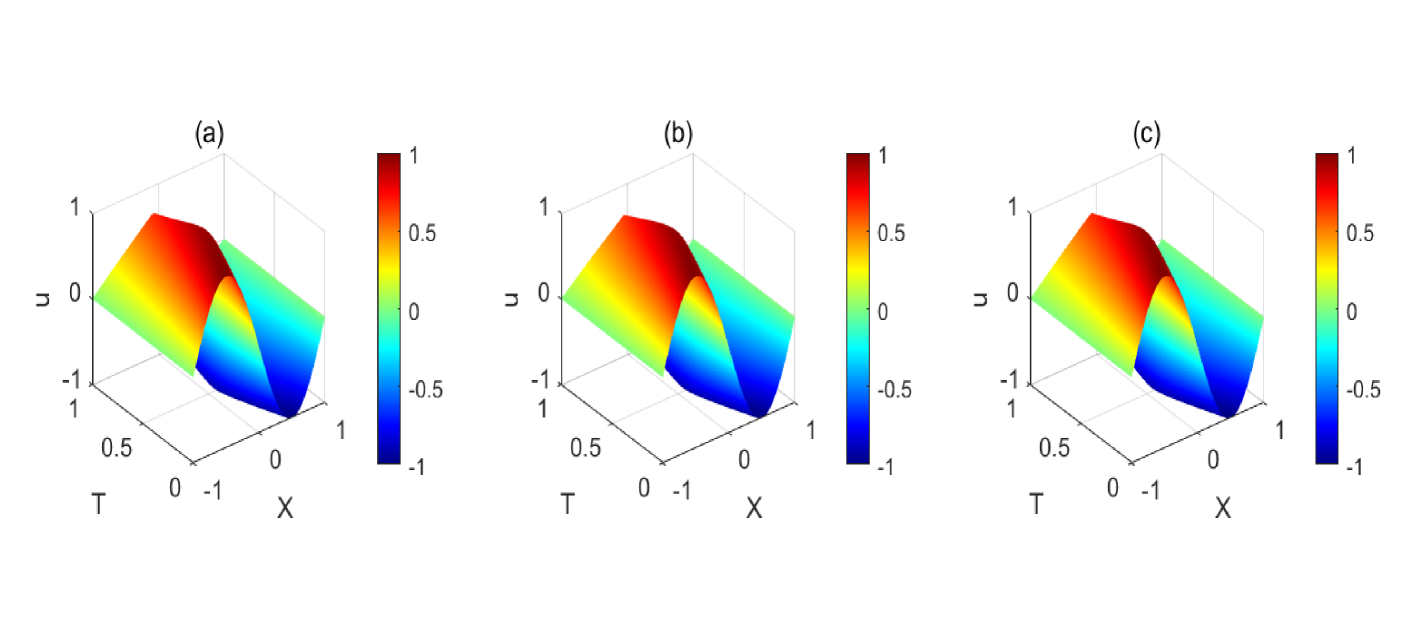
Figure 1: The solution $\mathbf{u}(t,\mathbf{x})$ of the Burgers’ equation when $\gamma=50\%$ (a) Reference solution. (b) The standard DMD predictive solution. (c) LDMD with adaptive partitioning solution.

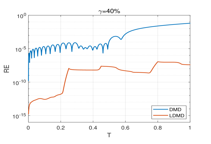
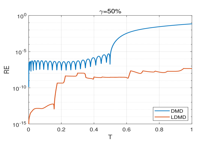
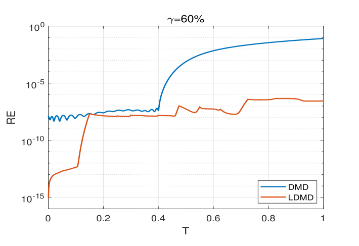
Figure 2: Model $L^{2}$ relative error in different prediction rates. From top to bottom prediction rates $\gamma$ are $40\%,50\%,60\%$ respectively.

Table 1: Comparison of CPU time and the mean $L^{2}$ relative errors of the Burgers’ for FOM, DMD, and LDMD at different prediction rates.

Model				CPU time(s)	$MRE$
FOM		4.2451	/
$\gamma=60\%$	DMD	2.2772	0.0157
	LDMD	1.9171	$1.1922\times 10^{-7}$
$\gamma=50\%$	DMD	2.0522	0.0125
	LDMD	1.7759	$9.7537\times 10^{-9}$
$\gamma=40\%$	DMD	1.7820	0.0111
	LDMD	1.4204	$2.1633\times 10^{-8}$

We use the implicit finite difference method as the FOM to solve the reference solution. Presented in Table 1 the CPU time in the FOM is about $4.2451s$, which is more expensive than data-driven methods. The computational efficiency and accuracy of LDMD with adaptive partitioning surpass those of the standard DMD method, with prediction performance improving as the prediction rate decreases. However, this also depends on the selection of the time window size and the upper bound of the residual.

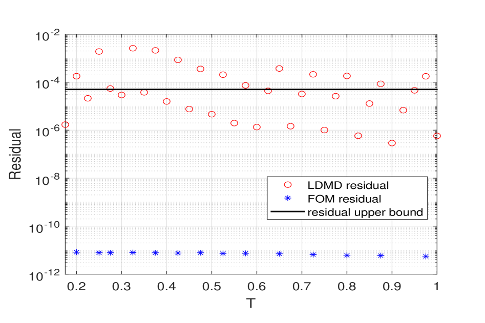
Figure 3: Residual of the LDMD with adaptive partitioning solution when $\gamma=50\%$.

Figure 1 shows that both the standard DMD and our LDMD with adaptive partitioning are able to approximate the Burgers’ equation well.

Actually, Figure 2 demonstrates our LDMD with adaptive partitioning almost always outperforms the standard DMD method in the different prediction rates. We can notice that the smaller the prediction rate, the more accurate our prediction results will be, and the improvement effect of the LDMD method will be more significant based on our reasonable selection of residual upper bound and time window size. The $RE$ of the LDMD method shows significant growth in the initial stage with relatively few snapshot data but quickly stabilizes between $10^{-9}$ and $10^{-7}$ after FOM correction. Instead, during the prediction phase, the $RE$ of the standard DMD continues to increase until about $10^{-1}$. In the reconstruction phase of the standard DMD method, the prediction results of our LDMD with adaptive partitioning are slightly better($\gamma=60\%$ or $50\%$) than or more than $2$ orders of magnitude better than the standard DMD method; In the prediction phase of the standard DMD method, the prediction results of our LDMD with adaptive partitioning are stable, and nearly up to $7$ orders of magnitude better than the standard DMD method.

As mentioned in algorithm 3, we start from the prediction part of the first stage, calculating the residuals every $m$ time steps, and applying the FOM to correct the portion in which the residual exceeds the given upper bound. This means the residual equation will be applied twice, resulting in two residual values at these moments. As expected, the residual is relatively large during the prediction time steps and continues to grow with each stage of prediction until it exceeds the given upper bound. After using FOM to correct the prediction result, the residual becomes very small shown in Figure 3.

5.2 Allen-Cahn equation

We consider the Allen-Cahn equation, a type of reaction-diffusion equation, with Neumann boundary conditions, which has a nonlinear equation source term and is used to describe phase separation and interface motion. It can be expressed as follows:

$$\begin{cases}{\frac{\partial\mathbf{u}}{\partial t}}=\alpha{\frac{\partial^{2}\mathbf{u}}{\partial x^{2}}}+5(\mathbf{u}-\mathbf{u}^{3}),\quad\mathbf{x}\in[-L,L],\quad t\in[0,T],\\ \mathbf{u}(0,\mathbf{x})=0.53\mathbf{x}+0.47\sin(-\frac{3}{2}\pi\mathbf{x}),\\ \frac{\partial\mathbf{u}(t,-L)}{\partial x}=\frac{\partial\mathbf{u}(t,L)}{\partial x}=0,\end{cases}$$ (5.2)

where $L=1$, $T=2$ and the diffusion coefficient $\alpha=10^{-4}$. Although the nonlinear source term dominates the dynamics, we let $g(\mathbf{u})=\mathbf{u}$. We set the spatial domain discretized into $N_{x}=200$ intervals, and the time domain discretized into $N_{t}=2000$ steps. Then, we set

$$r=15,\quad\epsilon=3\times 10^{-5},\quad n_{1}=200,\quad m=50.$$

So the prediction rate $\gamma=50\%$, correspondingly $M=1000$ in the standard DMD method.

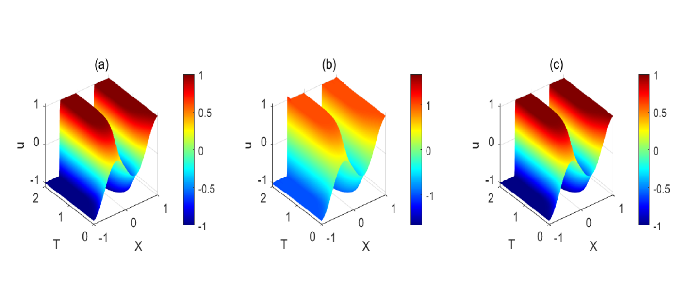
Figure 4: The solution $\mathbf{u}(t,\mathbf{x})$ of the Allen-Cahn equation (a) Reference solution. (b) The standard DMD predictive solution. (c) LDMD with adaptive partitioning solution.

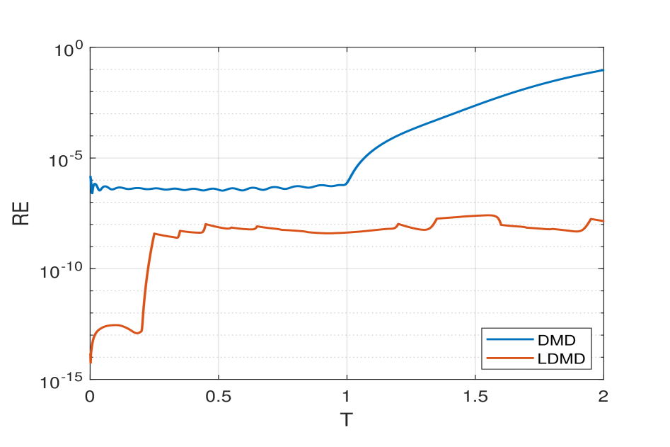
Figure 5: Model $L^{2}$ relative error.

We use the implicit finite difference method as the FOM to solve the reference solution. LDMD with adaptive partitioning can also achieve higher prediction accuracy and computation speed than the standard DMD method shown in Table 3.

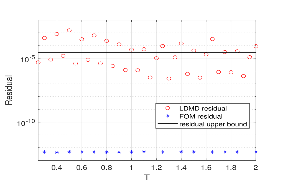
Figure 6: Residual of the LDMD with adaptive partitioning solution.

Figure 4 shows that our LDMD with adaptive partitioning performs well in approximating the reference solution, whereas the standard DMD method performs relatively poorly in comparison.

Figure 5 shows the $RE$ of the LDMD with adaptive partitioning is always below the standard DMD method. By reasonable selection of residual upper bound and time window size, in the reconstruction phase of the standard DMD method, the prediction result of our LDMD with adaptive partitioning is better than the standard DMD method up to $1$ order of magnitude. In the prediction phase of the standard DMD method, the prediction result of our LDMD with adaptive partitioning is stable between $10^{-9}$ and $10^{-7}$, and nearly up to $7$ orders of magnitude better than the standard DMD method.

Figure 6 shows a similar conclusion as Figure 3 that the residual is relatively large during the prediction time steps and continues to grow with each stage of prediction until it exceeds the given upper bound. After using FOM to correct the prediction result, the residual becomes very small.

5.3 Nonlinear Schrödinger equation

We consider one of the fundamental equations in quantum mechanics——the nonlinear Schrödinger equation(NLSE):

$$\begin{cases}\mathbf{\psi}_{t}-i\theta\mathbf{\psi}_{xx}-i\theta|\mathbf{\psi}|^{2}\mathbf{\psi}=0,\quad\mathbf{x}\in[-L,L],\quad t\in[0,T],\\ \mathbf{\psi}(0,\mathbf{x})=2\text{sech}(\mathbf{x}),\\ \mathbf{\psi}(t,-L)=\mathbf{\psi}(t,L)=0,\end{cases}$$ (5.3)

where $L=15$, $T=\pi$ and $\theta=0.5$. In this case, we also let $g(\mathbf{u})=\mathbf{u}$. We set the spatial domain discretized into $N_{x}=100$ intervals and the time domain discretized into $N_{t}=2000$ steps. The solution $\mathbf{\psi}(t,\mathbf{x})$ of the Schrödinger equation is a wave function, and we are concerned about its position density:

$$\mathbf{\rho}(t,\mathbf{x})=|\mathbf{\psi}(t,\mathbf{x})|^{2}.$$

Then, we set

$$r=10,\quad\epsilon=2\times 10^{-7},\quad n_{1}=50,\quad m=50.$$

So the prediction rate $\gamma=50\%$, correspondingly $M=1000$ in the standard DMD method.

Figure 7: The position density $\mathbf{\rho}(t,\mathbf{x})$ of the NLSE (a) Reference position density. (b) The standard DMD predictive position density. (c) LDMD with adaptive partitioning position density.

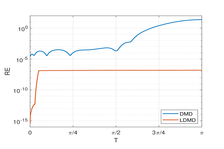
Figure 8: Model $L^{2}$ relative error.

Table 2: Comparison of CPU time and the mean $L^{2}$ relative errors of the NLSE for FOM, DMD, and LDMD at the prediction rate $\gamma=50\%$.

Model	CPU time(s)	$MRE$
FOM	0.1333	/
DMD	0.0695	3.5012
LDMD	0.0921	$1.4107\times 10^{-7}$

We use the spectral method as the FOM to solve the reference solution. Since the fast computational speed of the spectral method, it is faster compared to the standard DMD method, which performs repetitive calculations during certain periods. However, the $MRE$ of the LDMD method is much smaller shown in Table 2.

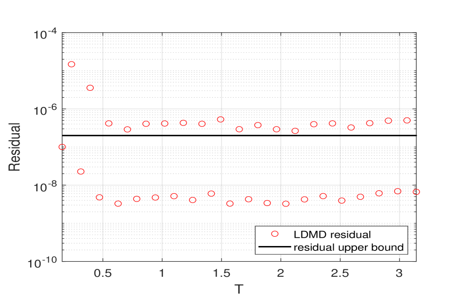
Figure 9: Residual of the LDMD with adaptive partitioning solution.

Figure 7 shows that the prediction error of the standard DMD method is significant, instead, our LDMD with adaptive partitioning can approximate the position density of the NLSE well. However, due to its oscillation characteristic, even if selecting appropriate observation functions, larger SVD truncation numbers, and more snapshot information, the prediction results remained unsatisfactory in the standard DMD method.

Figure 8 demonstrates our LDMD with adaptive partitioning always outperforms the standard DMD method. Our method gives a stable prediction result between $10^{-7}$ and $10^{-6}$ through a reasonable selection of residual upper bound and time window size, while the $RE$ of the standard DMD method is up to above $10$. However, the relative prediction error of the standard DMD rapidly increases and exceeds $10$ around $T=\pi$.

The residual is distributed above and below the residual boundary. Figure 9 indicates that the DMD prediction and the FOM correction are alternated. Different from Figure 3 and Figure 6, the residual equation we use corresponds to the FOM, so we have no numerical calculation errors when using the FOM to correct the prediction results.

5.4 Maxwell’s equations

Finally, we consider the time-domain Maxwell’s equations which are coupled systems used to the classical electromagnetic equations:

$$\begin{cases}\mathbf{curl}~\mathbf{E}(t,\mathbf{x})=-\frac{\partial(\mu_{r}\mathbf{H}(t,\mathbf{x}))}{\partial t},&\mathbf{x}\in\Omega,\quad t\in(0,T],\\ \mathbf{curl}~\mathbf{H}(t,\mathbf{x})=\frac{\partial(\varepsilon_{r}\mathbf{E}(t,\mathbf{x}))}{\partial t}+\mathbf{J}(t,\mathbf{x}),&\mathbf{x}\in\Omega,\quad t\in(0,T],\\ \frac{1}{\mu}\mathbf{curl}~\mathbf{E}(t,\mathbf{x})\times\mathbf{n}=0,&\mathbf{x}\in\partial\Omega,\quad t\in(0,T],\end{cases}$$ (5.4)

where $\mu_{r}$ and $\varepsilon_{r}$ are the relative electric permittivity and magnetic permeability respectively; $\mathbf{E}=(E_{x},E_{y},E_{z})^{T}$ is the electric field, $\mathbf{H}=(H_{x},H_{y},H_{z})^{T}$ is the magnetic field, $\mathbf{J}=(J_{x},J_{y},J_{z})^{T}$ is the dipolar current. In this case, we consider the 2-D time-domain case of transverse magnetic (TM) formulation, i.e. a scalar electric field $E=E_{z}$, a vector magnetic field $\mathbf{H}=(H_{x},H_{y})^{T}$, a scalar dipolar current $J=J_{z}$ [19, 20]; the differential operators are

$$\mathbf{curl}~E=(\frac{\partial}{\partial y}E,-\frac{\partial}{\partial x}E)^{T},\mathrm{curl}~\mathbf{H}=\frac{\partial}{\partial x}H_{y}-\frac{\partial}{\partial y}H_{x}.$$

and the initial conditions are given by

$$\mathbf{H}(0,\mathbf{x})=(0,0),\quad\mathbf{J}(0,\mathbf{x})=0,\quad\mathbf{E}(0,\mathbf{x})=\sin{\pi x}\cos{\pi y},$$

the spatial domain $\Omega=[0,1]\times[0,1]$, the time domain $T=2$. We perform triangulation in the spatial domain and the time domain discretized into $N_{t}=2000$ steps. According to Koopman operator theory, we choose the observable function $\mathbf{g}(\mathbf{u})=\left[\begin{matrix}\mathbf{u}\\ e^{\mathbf{u}}\end{matrix}\right]$. Since the difficulty of residual equation solution in coupled systems, we set

$$r=15,\quad n_{1}=90,\quad m_{1}=10,$$

in the first stage, and

$$n_{i}=50,\quad m_{i}=50,$$

in the following stages. So the prediction rate $\gamma=52\%\approx 50\%$, correspondingly $M=1040$ in the standard DMD method.

Since the electric and magnetic fields of Maxwell’s equation (5.4) are coupled under time-varying dynamic fields, using a single linear operator to describe the overall dynamics cannot explicitly establish the interaction mechanism between subsystems. We performed only a small portion of the predictions in the first stage to get a result with a small error as the initial value for FOM correction in the next stage.

We use the Discontinuous Galerkin as the FOM to solve the reference solution. Presented in Table 3 the CPU time in the FOM is about $294.5803s$. The CPU time in the DMD and LDMD is about half of the FOM, which corresponds to $\gamma\approx 50\%$. The computational efficiency and accuracy of LDMD surpass those of the standard DMD method greatly.

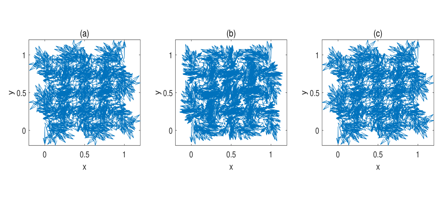
Figure 10: The magnetic field $\mathbf{H}$ of the Maxwell equation at $T=2$ (a) Reference magnetic field. (b) The standard DMD predictive magnetic field. (c) LDMD with predefined partitioning magnetic field.

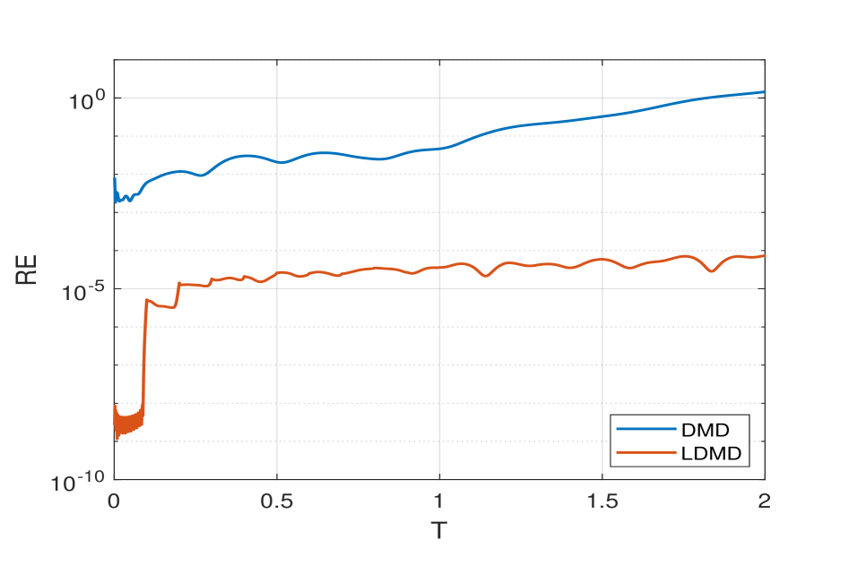
Figure 11: Model $L^{2}$ relative error of the magnetic field $\mathbf{H}_{y}$.

Figure 10, 12, and 14 show that the prediction error of the standard DMD method is significant, instead, our LDMD with adaptive partitioning can get better prediction results at $T=2$.

In the two-dimensional TM case, $H_{x}$ and $H_{y}$ have certain symmetry and expressions that can be expressed as the product of the sine function, cosine function, and exponential function. Therefore, the DMD prediction results for both are identical. We only exhibit $H_{y}$ in the numerical experiment and $H_{x}$ has the same prediction results.

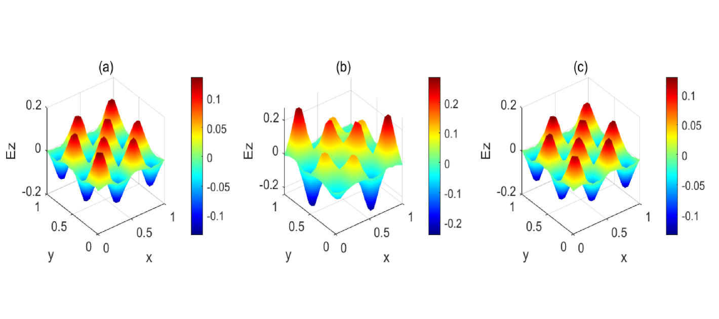
Figure 12: The electric field $E$ of the Maxwell equation at $T=2$ (a) Reference electric field. (b) The standard DMD predictive electric field. (c) LDMD with predefined partitioning electric field.

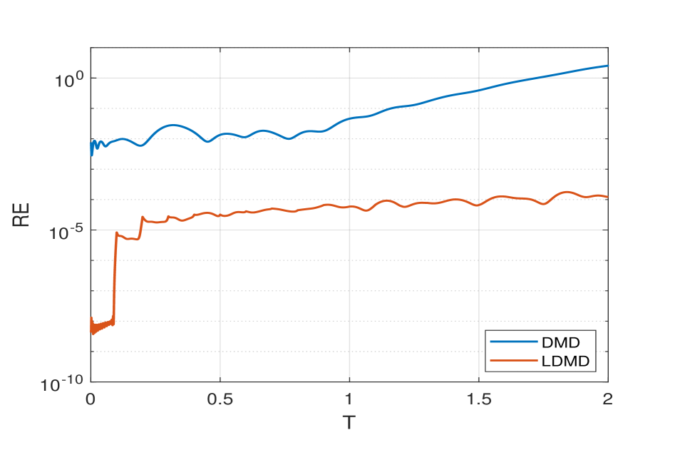
Figure 13: Model $L_{2}$ relative error of the electric field $E_{z}$.

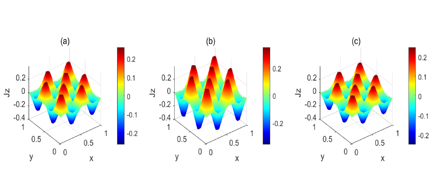
Figure 14: The dipolar current $J$ of the Maxwell equation at $T=2$ (a) Reference dipolar current. (b) The standard DMD predictive dipolar current. (c) LDMD with predefined partitioning dipolar current.

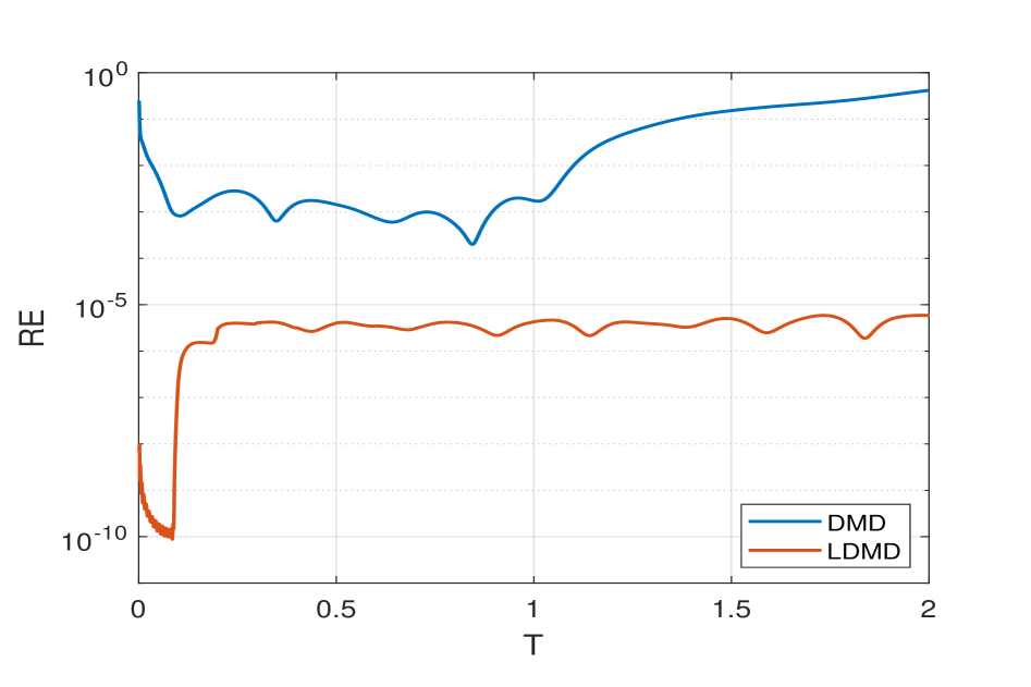
Figure 15: Model $L^{2}$ relative error of the dipolar current $J_{z}$.

In the coupled system, we selected small snapshot data in the first stage, which will result in a rapid increase in the prediction error of our subsequent DMD. To address this, we limited the number of prediction time steps in the first stage, ensuring that the subsequent prediction results remained relatively stable and that the error did not increase too rapidly. Presented in Figure 11 and Figure 13 our LDMD method has shown a slight increase in $RE$, but overall it can remain stable at around $10^{-5}$. Figure 15 shows that the $RE$ is stable below $10^{-5}$. On the contrary, the standard DMD method exhibits a high $RE$ even in the reconstruction phase, and the $RE$ may exceed $1$ during the subsequent prediction process, leading to unsatisfactory results. In general, our LDMD method is better than the standard DMD method by about $2$ orders of magnitude or more in the reconstruction phase of the standard DMD method and about $4$ orders of magnitude or more at $T=2$.

Table 3: Comparison of CPU time and the mean $L^{2}$ relative errors for FOM, DMD, and LDMD at the prediction rate $\gamma=50\%$ or $\gamma\approx 50\%$.

Model					CPU time(s)	$MRE$
Burgers’ equation	FOM	4.2451	/
	DMD	2.0522	0.0125
	LDMD	1.7759	$9.7537\times 10^{-9}$
Allen-Cahn equation	FOM	52.3481	/
	DMD	26.7059	0.0076
	LDMD	18.1453	$7.5795\times 10^{-9}$
Maxwell’s equations	FOM	294.5803	/
	DMD	150.0453	magnetic field	0.2614
			electric filed	0.3594
			dipolar current	0.0801
	LDMD	158.5724	magnetic field	$3.3659\times 10^{-5}$
			electric filed	$6.4252\times 10^{-5}$
			dipolar current	$3.5211\times 10^{-6}$

At last, we provide the CPU time of the Burgers’ equation, Allen-Cahn equation, and Maxwell’s equations under FOM, DMD, and LDMD algorithms and the $MRE$ comparison between our LDMD method and the standard DMD method at the prediction rate $\gamma=50\%$ shown in Table 3. Since the low-rank approximation core of DMD is the SVD truncation, our LDMD method is a localized method, meaning the matrix dimension of the SVD applied at each stage is smaller than that in the standard DMD. This makes it more computationally efficient and time-saving, even with repeated calculations during certain periods. The $MRE$ of our LDMD method is much smaller than the standard DMD method.

6 Conclusions

In this work, we have proposed the LDMD method, which integrates the standard DMD framework with a time-domain decomposition approach to address the limitations of standard DMD in long-term predictions for complex dynamical systems. We first proposed LDMD with predefined partitioning, which is straightforward to implement but relies on prior knowledge of the system to achieve higher accuracy. To overcome this limitation, we further developed LDMD with adaptive partitioning, which leverages an error estimator for control and operates without requiring prior observations of the system. This adaptive strategy determines whether the prediction error reaches its upper bound by evaluating each time window rather than at every time step, significantly improving its practical applicability. Numerical results demonstrate that, compared to the standard DMD method, our LDMD method achieves higher prediction accuracy, improved computational efficiency, and greater robustness. This advantage arises because dynamical systems are more likely to exhibit linear behavior over shorter time intervals. Notably, the relative error of the LDMD method stabilizes quickly at a lower level, whereas the prediction error of standard DMD continues to accumulate over time.

For future research, we aim to develop a more effective error estimator that aligns with the equation-free nature of DMD, ensuring broader applicability, computational simplicity, and the ability to correct inaccurate predictions for subsequent stages. Additionally, we seek to provide a comprehensive and rigorous theoretical analysis comparing LDMD with standard DMD, demonstrating that LDMD consistently outperforms standard DMD across all time intervals by optimizing the time window size and error estimator threshold. Ultimately, we aspire to establish LDMD as a high-accuracy surrogate model for parametric dynamical systems, further enhancing the predictive capabilities of existing methodologies [35, 21].

References

- [1] H. Arbabi and I. Mezić, Ergodic theory, dynamic mode decomposition, and computation of spectral properties of the Koopman operator, SIAM J. Appl. Dyn. Syst., 16 (2017), pp. 2096-2126.
- [2] T. Askham and J. N. Kutz, Variable projection methods for an optimized dynamic mode decomposition, SIAM J. Appl. Dyn. Syst., 17 (2018), pp. 380-416.
- [3] S. L. Brunton, B. W. Brunton, J. L. Proctor, and J. N. Kutz, Koopman invariant subspaces and finite linear representations of nonlinear dynamical systems for control, PloS One, 11 (2016), e0150171.
- [4] K. K. Chen, J. H. Tu, and C. W. Rowley, Variants of dynamic mode decomposition: Boundary condition, Koopman, and Fourier analyses, J. Nonlinear Sci., 22 (2012), pp. 887-915.
- [5] S. Le Clainche and J. M. Vega, Higher order dynamic mode decomposition, SIAM J. Appl. Dyn. Syst., 16 (2017), pp. 882-925.
- [6] D. Duke, J. Soria, and D. Honnery, An error analysis of the dynamic mode decomposition, J. Exp. Fluids, 52 (2012), pp. 529-542.
- [7] D. Dylewsky, M. Tao, and J. N. Kutz, Dynamic mode decomposition for multiscale nonlinear physics, Phys. Rev. E, 99 (2019), pp. 063311.
- [8] S. A. Falconer, D. J. B. Lloyd, and N. Santitissadeekorn, Combining dynamic mode decomposition with ensemble Kalman filtering for tracking and forecasting, Phys. D, 449 (2023), pp. 133741.
- [9] R. Ghosh and M. Mcafee, Koopman operator theory and dynamic mode decomposition in data-driven science and engineering: A comprehensive review, Mathematical Modelling and Numerical Simulation with Applications, 4 (2024), pp. 562-594.
- [10] P. S. Heckbert and M. Garland, Survey of polygonal surface simplification algorithms, Siggraph, 1997.
- [11] T. T. P. Hoang, J. Jaffré, C. Japhet, M. Kern, and J. E. Roberts, Space-time domain decomposition methods for diffusion problems in mixed formulations, SIAM J. Numer. Anal., 51 (2013), pp. 3532-3559.
- [12] L. Ji, Z. Peng, and Y. Chen, AAROC: Reduced Over-Collocation Method with Adaptive Time Partitioning and Adaptive Enrichment for Parametric Time-Dependent Equations, preprint, arXiv:2412.02152, 2024.
- [13] J. Jiang and Y. Chen, Adaptive greedy algorithms based on parameter‐domain decomposition and reconstruction for the reduced basis method, Internat. J. Numer. Methods Engrg., 121 (2020), pp. 5426-5445.
- [14] M. Korda and I. Mezić, On convergence of extended dynamic mode decomposition to the Koopman operator, J. Nonlinear Sci., 28 (2018), pp. 687-710.
- [15] J. N. Kutz, S. L. Brunton, B. W. Brunton, and J. L. Proctor, Dynamic mode decomposition: data-driven modeling of complex systems, Other Titles Appl. 149, SIAM, Philadelphia, 2016.
- [16] J. N. Kutz, X. Fu, and S. L. Brunton, Multiresolution dynamic mode decomposition, SIAM J. Appl. Dyn. Syst., 15 (2016), pp. 713-735.
- [17] J. N. Kutz, J. L. Proctor, and S. L. Brunton, Applied Koopman Theory for Partial Differential Equations and Data-Driven Modeling of Spatio-Temporal Systems, Complexity, 2018 (2018), pp. 6010634.
- [18] M. Lee and J. Park, An optimized dynamic mode decomposition model robust to multiplicative noise, SIAM J. Appl. Dyn. Syst., 22 (2023), pp. 235-268.
- [19] K. Li, T. Z. Huang, L. Li, and S. Lanteri, A reduced-order DG formulation based on POD method for the time-domain Maxwell’s equations in dispersive media, J. Comput. Appl. Math., 336 (2018), pp. 249-266.
- [20] K. Li, T. Z. Huang, L. Li, Y. Zhao, and S. Lanteri, A non-intrusive model order reduction approach for parameterized time-domain Maxwell’s equations, Discrete Contin. Dyn. Syst. Ser. B, 28 (2022), pp. 449-473.
- [21] Q. Li, C. Liu, M. Li, and P. Zhang, An Adaptive Method Based on Local Dynamic Mode Decomposition for Parametric Dynamical Systems, Commun. Comput. Phys., 35 (2024), pp. 38-69.
- [22] M. Lovrić, M. Milanović, and M. Stamenković, Algoritmic methods for segmentation of time series: An overview, Journal of Contemporary Economic and Business Issues, 1 (2014), pp. 31-53.
- [23] H. Lu and D. M. Tartakovsky, Prediction accuracy of dynamic mode decomposition, SIAM J. Sci. Comput., 42 (2020), pp. A1639-A1662.
- [24] E. J. Keogh and M. J. Pazzani, An enhanced representation of time series which allows fast and accurate classification, clustering and relevance feedback., Kdd, 98 (1998), pp. 239-243.
- [25] A. Koski, M. Juhola, and M. Meriste, Syntactic recognition of ECG signals by attributed finite automata, Pattern Recognition, 28 (1995), pp. 1927-1940.
- [26] B. Lusch, J. N. Kutz, and S. L. Brunton, Deep learning for universal linear embeddings of nonlinear dynamics, Nature communications, 9 (2018), pp. 4950.
- [27] I. Mezić, Analysis of fluid flows via spectral properties of the Koopman operator, Annu. Rev. Fluid Mech., 45 (2013), pp. 357-378.
- [28] R. Ouda and P. Hart, Pattern classification and scene analysiswiley, New York, 1973.
- [29] J. L. Proctor, S. L. Brunton, and J. N. Kutz, Dynamic mode decomposition with control, SIAM J. Appl. Dyn. Syst., 15 (2014), pp. 142-161.
- [30] C. W. Rowley, I. Mezić, S. Bagheri, P. Schlatter, and D. S. Henningson, Spectral analysis of nonlinear flows, J. Fluid Mech., 641 (2009), pp. 115-127.
- [31] J. A. Rosenfeld and R. Kamalapurkar, Singular dynamic mode decomposition, SIAM J. Appl. Dyn. Syst., 22 (2023), pp. 2357-2381.
- [32] P. J. Schmid, Dynamic mode decomposition of numerical and experimental data, J. Fluid Mech., 656 (2010), pp. 5-28.
- [33] P. J. Schmid, Application of the dynamic mode decomposition to experimental data, Exp. Fluids, 50 (2011), pp. 1123-1130.
- [34] P. J. Schmid, Dynamic mode decomposition and its variants, Annu. Rev. Fluid Mech., 54 (2022), pp. 225-254.
- [35] H. Song, Y. Ba, D. Chen, and Q, Li, A model reduction method for parametric dynamical systems defined on complex geometries, J. Comput. Phys., 506 (2024), pp. 112923.
- [36] F. Takens, Detecting strange attractors in turbulence, Springer, 2006, pp. 366–381.
- [37] J. H. Tu, C. W. Rowley, D. M. Luchtenburg, S. L. Brunton, and J. N. Kutz, On dynamic mode decomposition: Theory and applications, J. Comput. Dyn., 1 (2014), pp. 391-421.
- [38] M. O. Williams, C. W. Rowley, and I. G. Kevrekidis, A kernel-based method for data-driven Koopman spectral analysis, J. Comput. Dyn., 2 (2015), pp. 247-265.
- [39] M. O. Williams, I. G. Kevrekidis, and C. W. Rowley, A data-driven approximation of the Koopman operator: Extending dynamic mode decomposition, J. Nonlinear Sci., 25 (2015), pp. 1307-1346.
- [40] S. Wu and T. Zhou, Parareal algorithms with local time-integrators for time fractional differential equations, J. Comput. Phys., 358 (2018), pp. 135-149.
- [41] S. Wu and T. Zhou, Acceleration of the two-level MGRIT algorithm via the diagonalization technique, SIAM J. Sci. Comput., 41 (2019), pp. A3421-A3448.
- [42] S. Wu and T. Zhou, Convergence Analysis of the Parareal Algorithm with Nonuniform Fine Time Grid, SIAM J. Numer. Anal., 62 (2024), pp. 2308-2330.
- [43] Y. Yin, C. Kou, and S. Jia, PCDMD: Physics-constrained dynamic mode decomposition for accurate and robust forecasting of dynamical systems with imperfect data and physics, Comput. Phys. Comm., 304 (2024), pp. 109303.