A Downstream and vertexing algorithm for Long Lived Particles (LLP) selection at the first High level trigger (HLT1) of LHCb

Abstract

A new algorithm has been developed at LHCb which is able to reconstruct and select very displaced vertices in real time at the first level of the trigger (HLT1). It makes use of the Upstream Tracker (UT) and the Scintillator Fiber detector (SciFi) of LHCb and it is executed on GPUs inside the Allen framework. In addition to an optimized strategy, it utilizes a Neural Network (NN) implementation to increase the track efficiency and reduce the ghost rates, with very high throughput and limited time budget. Besides serving to reconstruct ${K}^{0}_{\mathrm{\scriptscriptstyle S}}$ and $\mathchar 28931\relax$ particles from the Standard Model, the Downstream algorithm and the associated two-track vertexing could largely increase the LHCb physics potential for detecting long-lived particles during the Run 3.

1 Introduction

The LHCb forward spectrometer is one of the main detectors at the Large Hadron Collider (LHC) accelerator at CERN, with the primary purpose of searching for new physics through studies of CP-violation and heavy-flavour hadron decays. It has been operating during its Run 1 (2011-2012) and Run 2 (2015-2018) periods with very high performance, recording an integrated luminosity of 9 $\text{fb}^{-1}$ at center-of-mass energies of 7, 8, and 13 TeV and delivering a plethora of accurate physics results and new particles discoveries. One of the main issues concerning the present Run 3 was that, even if many physics results are statistically limited, a direct increase of the luminosity provided by the accelerator was not directly translated into an increase of the selected events of interest, and a new full-software-based selection (trigger) strategy was necessary CERN-LHCC-2020-006 . This new trigger paradigm has been very successful allowing LHCb to collect 10 $\text{fb}^{-1}$ at 13 TeV during 2023-2024. Due to the computing timing constraints, during previous runs the first stage of the trigger was based on fast partial particle tracking reconstruction, not including downstream trackers, since the large hit occupancy made the throughput decrease by two orders of magnitude. At that time Intel Xeon E5-2630 v3 CPUs were used for performing the reconstruction and selection tasks. A new algorithm called Downstream has been developed in this work, which makes use of the new trigger scheme based on A5000 NVIDIA GPUs,

1.1 The LHCb detector

The upgraded LHCb detector, operational at present during the Run 3 of the LHC, has implied a major change in the experiment. The detectors have been almost completely renewed to allow running at an instantaneous luminosity five times larger than that of the previous running periods, in particular using new readout architectures. A full software trigger executed on Graphic Processor Units (GPU) also represents one of the main features of the new LHCb design, allowing the reconstruction and selection of events in real-time and widening the physics reach of the experiment. The main characteristics of the new LHCb detector are detailed in Aaij_2024 , and summarised in the following. As compared to the previous detector LHCb_2008 , one of the most important improvements concerns the new tracking system. The LHCb is comprised of a three subdetector tracking system (VErtex LOcator, Upstream Tracker, and SciFi tracker), a particle identification system, based on two-ring imaging Cherenkov detectors, hadronic and electromagnetic calorimeters, and four muon chambers.

The VErtex LOcator (VELO) is based on pixelated silicon sensors and is critical for determining the decay vertices of $b$ and $c$ flavored hadrons. The Upstream Tracker (UT) contains vertically segmented silicon strips and continues the tracking upstream of the VELO. It is also used to determine the momentum of charged particles and is useful to remove low-momentum tracks from being extrapolated downstream, thus speeding up the software trigger by about a factor of three. Tracking after the magnet is handled by the new scintillating fiber-based Scintillating Fiber detector (SciFi). Two Ring Imaging Cherenkov (RICH) detectors supply particle identification. RICH1 is mainly for lower momentum particles, and RICH2 is for higher momentum ones. The Electromagnetic Calorimeter (ECAL) identifies electrons and reconstructs photons and neutral pions. The Hadronic Calorimeter (HCAL) measures the energy deposits of hadrons, and four muon chambers M2-M5 are mostly used for muon identification. The angular coverage of the LHCb detectors ranges from $2<\eta<5$. Figure 1 shows the LHCb upgrade detector.

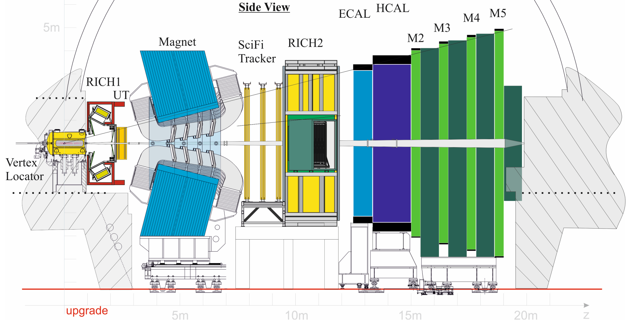
Figure 1: The new LHCb detector operating during the Run 3 Aaij_2024 . The LHCb coordinate system is a right-handed cartesian system with the $z$ axis aligned with the beamline and pointing downstream the detector, and the $y$ axis pointing upwards.

Figures of the main detectors involved in the Downstream algorithm are also shown in Fig. 2 and Fig. 3.

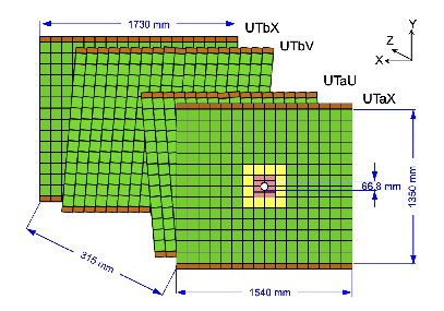
Figure 2: Sketch of the four silicon planes which is composed of UT detector with indicative dimensions. The first (”a”) station is composed of an $x$-measuring layer (UTaX) with vertical strips and a stereo layer (UTaU) with strips inclined by $5^{\circ}$. The second (”b”) station is similar, with first a stereo layer (UTbV) with opposite inclination, and a layer with vertical strips (UTbX) Aaij_2024 .

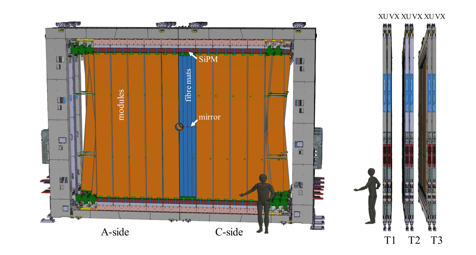
Figure 3: Front and side views of the SciFi detector. Twelve detection planes are arranged in three stations with 4 layers each in an $X-U-V-X$ configuration. The $X$ layers have their scintillator fibres oriented vertically and are used for determining the deflection of the charged particle tracks caused by the magnetic field. The inner two stereo layers, $U$ and $V$, have their fibres rotated by $\pm 5^{\circ}$ in the plane of the layer for reconstructing the vertical position of the track hit Aaij_2024 .

.

1.2 Track types at LHCb

The tracking system of the LHCb experiment consists of three subsystems, VELO, UT, and SciFi, which are responsible for reconstructing charged particles. A magnet, with a bending power of 4 Tm, is also necessary to curve particle trajectories in order to measure their momentum, $p$. Its polarity can be inverted, and it is used to control systematic effects coming from detector inefficiencies.

Several track types are defined depending on the subdetectors involved in the reconstruction, as shown in Fig. 4.

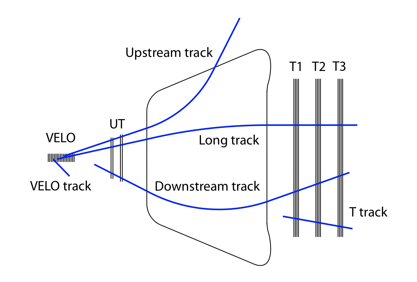
Figure 4: Definition of the particle track types in the LHCb experiment, according to which detectors are hit. The different tracker layers and the magnet in the center are sketched.

The main track types considered for physics analyses are

• Long tracks: they have information from at least the VELO and the SciFi, and possibly the UT. These are the main tracks used in physics analyses and at all stages of the trigger;
  

• Downstream tracks: they have information from the UT and the SciFi, but not VELO. They typically correspond to decay products of ${K}^{0}_{\mathrm{\scriptscriptstyle S}}$ and $\mathchar 28931\relax$ hadron decays;
  

• T tracks: they only have hits from the SciFi. They are typically not included in physics analysis. Nevertheless, their potential for physics has been recently probed arXiv:2211.10920 ; Svintozelskyi:2914251 .

When simulating collision data, particle tracks meeting certain thresholds are defined to be reconstructible and have an assigned type according to the sub-detector reconstructibility. This is, in turn, based on the existence of reconstructed detector digits or clusters in the emulated detector, which are matched to simulated particles Li:2752971 . Requirements for long tracks imply VELO and SciFi reconstructibility, downstream tracks must satisfy the UT and SciFi reconstructibility, and T-tracks only require the SciFi one.

1.3 The HLT1 trigger

The trigger system of the LHCb detector in Run 3 is software based and comprises two levels: HLT1 and HLT2, described in detail in Ref. CERN-LHCC-2014-016 ; CERN-LHCC-2020-006 . The HLT1 level has to be executed at a 30 MHz rate and, as such, suffers from heavy constraints on timing for event reconstruction. It performs partial event reconstruction in order to reduce the data rate. Tracking algorithms play a key role in fast event decisions, and the fact that they are inherently parallelisable processes suggests a way to increase trigger performance. Thus, the HLT1 has been implemented on a number of GPUs within the Allen software project Aaij:2019zbu , which allows to manage 4 TB/s and reduces the data rate by a factor of 30. After this initial selection, data is passed to a buffer system, which allows nearly real-time calibration and alignment of the detector. This is used for the full and improved event reconstruction carried out by HLT2.

Due to timing constraints, the LHCb implementation in the HLT1 stage has been based on partial reconstruction and focuses solely on long tracks, i.e., tracks that have hits in the VELO. This trigger thus significantly affects the identification of particles with long lifetimes, particularly for LLP searches in LHCb, where some of the final-state particles are created further than roughly a metre away from the IP and thus outside of the VELO acceptance. A new algorithm Jashal:2881886 has been developed and implemented to widen the reach of particle lifetimes of the HLT1 system.

2 The Downstream algorithm

Downstream is a fast and performant algorithm designed to reconstruct tracks which do not have hits in the VELO detector. In the following the design of the algorithm and its performance are described.

2.1 Algorithm design

The algorithm is based on the extrapolation of SciFi seeds (or tracklets) to the UT detector, including the effect of the magnetic field in the $x$ direction. Only seeds that have not been used for long track reconstruction are considered as downstream candidates. In Fig. 5 the flow chart of the algorithm is outlined.

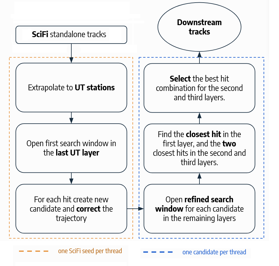
Figure 5: Flow chart of the Downstream algorithm (Dv0).

SciFi tracklets are obtained using a standalone algorithm called HybridSeeding HybridSeeding , modified for GPU execution in parallel. It performs a pattern recognition in the $x-z$ plane based on the triplet-search approach and then confirms the initial track by adding the $y$ information from the two $\pm 5^{\circ}$ tilted SciFi layers. Since each layer contains an average number of 400 hits, the algorithm copes with $400^{3}$ hit combinations to make the tracks. A constraint imposing the track originates from the (0,0,0) point reduces the number of tracklets to about 100. Removing the ones that have been used in the long track reconstruction, the initial tracklets for the Downstream algorithm can be around 20.

The change in the track direction by the magnetic field $\vec{B}$ is governed by the equation of motion

$$\frac{d\vec{p}}{dt}=q\vec{v}\times\vec{B},$$ (1)

with $\vec{p}$, $q$ and $\vec{v}$ being the momentum, charge, and velocity of the particle. At LHCb, the magnetic field is predominantly in the $y$ direction, causing track deviations in the $x-z$ plane. This is modeled by a kink at a given position in the $z$-axis (magnet point). This point is parameterised using the coordinates ($x$, $y$) and the track slopes ($t_{x},t_{y}$), where $t_{x}=px/pz=dx/dz$ and $t_{y}=py/pz=dy/dz$, of the seeds in the last SciFi station. An initial $q/p$ estimation also enters in the computation. Parameters are obtained by minimizing the difference between the predicted and true values of $z_{magnet}$ using simulated samples. The coordinates $x_{magnet}$ and $y_{magnet}$ are then calculated by straight-line extrapolation from SciFi, where a correction depending on the position and slope of the track is applied to correct the non-zero magnetic field in $x$ and $z$. In Fig. 6 the distribution of the bias vs the $z_{magnet}$ is shown from simulated events.

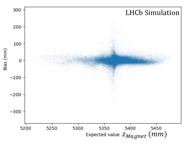
Figure 6: Distribution of the bias in $z_{Magnet}$.

• In a first version of the algorithm (Dv0) a search window for compatible hits is opened in the last layer of the UT ($UTbX$) (see Fig. 2). Tolerance regions in the UT are defined for each SciFi track, based on simulation studies and including the effect of the magnetic field. For each hit in the search window of the last UT layer a new trajectory is computed using $z_{magnet}$, and extrapolated to the remaining layers of the UT ($UTaX$,$UTaU$,$UTbV$), opening new tolerance windows. The closest hit in the first layer ($UTaX$) and the two closest ones in the second and third UT layers ($UTaU$,$UTbV$) are considered to make downstream candidates. Up to 10 best hits are selected in the initial $UTbX$ layer, and the tracklets without any matched hits in this layer are skipped.
  

• An improved version of the algorithm (Dv1) aiming for the reconstruction of new unknown particles with large masses, is also being developed. Assuming that downstream tracks point to the origin of the coordinate system in the definition of the first search window may have a negative impact on the tracking efficiency for decays where tracks have very large opening angles. Therefore, an initial tracking step with a triplet search algorithm is applied to increase the efficiency of heavy particle decays which involve large opening angles. Once the magnet point ($x_{magnet}$, $y_{magnet}$, $z_{magnet}$) is computed for each SciFi tracks, a parallelizes triplet search is performed along with the hits in the $UTaX$ and $UTbX$ layers of the UT to create downstream candidates.

  To optimize the throughput in this computationally-expensive new configuration, UT hits are grouped into different $Y$ sectors. Each SciFi track searches only for hits within compatible $Y$ sectors, under the assumption that there is no magnetic field component in the $X$ or $Z$ directions. Once the triplet is defined in the axial layers of the UT, hits from the stereo layers ($UTaU$ and $UTbV$) are added, and downstream tracks are constructed similarly to the Dv0 of the algorithm,

  The new Downstream version improves the tracking efficiency for decays of heavy BSM particles up to a factor of $4$, and removes any mass dependence. It also enhances the efficiency for ${K}^{0}_{\mathrm{\scriptscriptstyle S}}$ and $\mathchar 28931\relax$ byabout $20{\%}$ and $10{\%}$, respectively. It is still under development and will be tested during the 2025 data-taking. Figure 15 shows the efficiency improvement for a new particle with a mass of 3 GeV mass and 2 ns lifetime.

A final candidate is considered for each SciFi track based on the best combinations of hits according to a score computed with the distance between expected hit position and real hit position. This is achieved through a clone killing mechanism, which removes duplicate tracks that may have been created due to multiple hits associated with the same track. Iterating over all possible track pairs that have more than two shared UT hits or has the same SciFi segment, the candidates with lower scores are killed. This removes about 1% of the candidates.

One of the main features of the Downstream algorithm is the rejection of ghost tracks, which are fake tracks originated by spurious hits in the detector. This is explained in the following section.

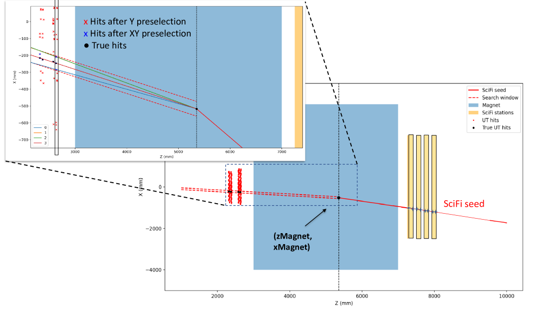
Figure 7: Strategy of the Downstream algorithm showing the used hits in the last UT layer and the Magnet Point ( $\ignorespaces x_{\text{Magnet}}$ , $\ignorespaces z_{\text{Magnet}}$ ) which is used to find the slope $t_{x}$. The slope is essentially the change in the $x$ position of the particle with respect to the change in the $z$ position from the Magnet Point to the UT stations.

Figure 7 shows an sketch of the algorithm strategy.

2.2 Ghost-killer Neural Network

Ghost tracks arise due to detector noise or reconstruction ambiguities. To suppress these tracks a streamlined feed-forward neural network (FFNN) with a unique hidden layer is used. The architecture includes as input six variables with information of the downstream track state ($x$,$y$,$t_{x}$,$t_{y}$,$q/p$,$\chi^{2}$), with $t_{i}$ the slope parameter (=$di/dz$), and $\chi^{2}$ a quantity to evaluate the goodness of the track fit. Information of the SciFi track properties ($q/p$ and $\chi^{2}$) are also included, completing eight input variables. A hidden layer with a $ReLu$ activation function lederer2021 and 14 neurons is used. The optimal number of neurons in the hidden layer is obtained by studying the ghost rejection rate vs the throughput of the algorithm. A Sigmoid function lederer2021 is used for the output to define a ghost probability score. Figure 8 shows the Ghost-killer architecture.

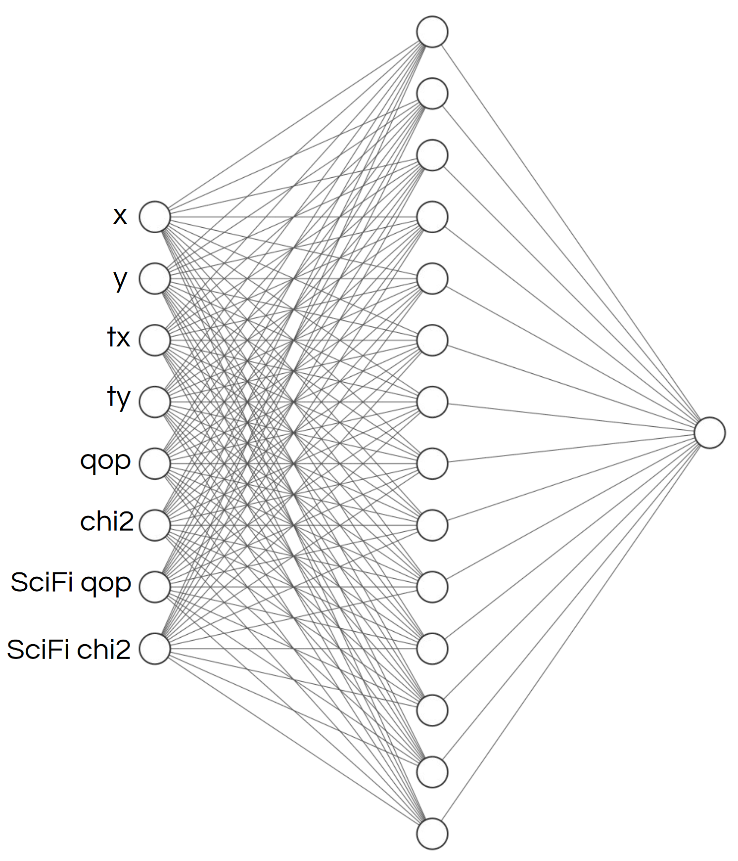
Figure 8: Architecture of the FFNN used to remove ghost tracks.

The training of the FFNN is performed using 10k $Bs\rightarrow\phi\phi$ simulated events, and the Adam optimisation algorithm kingma2017 with the binary cross-entropy loss function. The loss is defined as:

$$-\frac{1}{N}\sum_{i=1}^{N}\left[y_{i}\log(f(\mathbf{x}_{i}))+(1-y_{i})\log(1-f(\mathbf{x}_{i}))\right]$$

where $y_{i}$ is the true label of the $i$-th example (1 for ghost, 0 for real track) and $f(\mathbf{x}_{i})$ is the output of the NN for the $i$-th example. The loss values in the final epoch ($\approx 18000$) for both the test sample and train samples are found to be compatible. In Fig. 9 the classifier output for the Ghost-killer is shown.

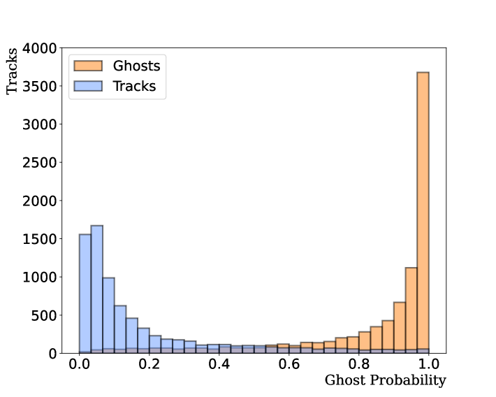
Figure 9: Probability score given by the FFNN output.

2.3 GPU implementation

The algorithm is almost entirely executed in order 500 hundreds A5000 NVIDIA GPUs, which are hosted in up to 190 AMD EPYC dual-socket servers with 32 physical cores and 512 GB of RAM per socket. The CPUs are responsible for data copying and other supplementary services.

To take advantage of multi-threading in the GPU, data is processed in slices of events, each slice processing between 500 and 1000 events. Each CUDA thread block is mapped to a single event in the slice, and each thread within the block works on an independent candidate for reconstruction or selection.

Threads within the same block can synchronize and share resources through shared memory. An RTX A5000 features 64 Streaming Multiprocessors (SMs), each containing 128 CUDA cores, for a total of 8,192 CUDA cores. That means that 64 events can be processed in parallel.

Given the large hit combinatorics in the SciFi and UT detectors for making the track candidates, and the tight throughput constraints of the HLT1 sequence, the speed of the algorithm is mandatory.

In order to achieve this, static structures are used in the Ghost-killer NN architecture definition, fixing the number of input variables and the number of neurons. This allows the compiler to perform compile-time optimizations, such as utilizing registers instead of global memory, thereby improving the efficiency and performance of the implementation.

Additional loop unrolling techniques are employed to mitigate the bottlenecks of $for$-loops by explicitly writing out each iteration. This is achieved using the NVCC-specific #pragma unroll directive, which allows for partial or complete unrolling of loops. Fast mathematical functions from the CUDA library, such as _fdividef and _expf, are also utilized to accelerate floating-point operations. These functions are approximations, but they ensure the precision requirements of our use case. Furthermore, shared memory is leveraged to cache hits that are accessed multiple times during the combinatorics, reducing the overhead of repeated global memory accesses. In the following section, the performance of the algorithm is detailed.

2.4 Algorithm performance

The performance of track reconstruction of Downstream is evaluated using several figures of merit, in particular, throughput, momentum resolution, physics efficiency and ghost rejection. The throughput is evaluated, during the development phase, using a sample of simulated minimum bias proton-proton collisions which represent the collisions and detector response as in real data. The momentum resolution, physics efficiency and ghost rejection are evaluated using a bunch of dedicated simulated samples, which are representative of beauty, charm and strange, meson and baryon decays.

Results are validated using the data acquired by the LHCb during October 2024, with the UT running in global conditions and the Downstream algorithm included in the HLT1 sequence.

Tracks of interest in physics events are expected to have momentum above 5 GeV/c and transverse momentum $p_{T}$ above 0.5 GeV/c. These criteria are applied to determine the performance of Downstream.

An additional figure of merit correlated to the throughput is the power consumption of the algorithm. Sustainability is a subject which is taking increasing attention in view of the next generation of experiments and the need to analyze big amount of data. In this work we have evaluated the relative increase in power consumption of Downstream, in order to try to minimize it.

2.4.1 Throughput

In Fig. 10 the performance of Downstream in terms of throughput is presented. It is related to the two reconstruction algorithms in the Allen sequence that determine long tracks: the Matching and Forward forward algorithms. The minimal required throughput per GPU card for the LHCb HLT1 system is 60kHz. The inclusion of Downstream in HLT1 slightly reduces the throughput in about 5 kHz for simulated and real data, when it is executed on a RTX A5000 card, as it can be seen in Fig. 10.

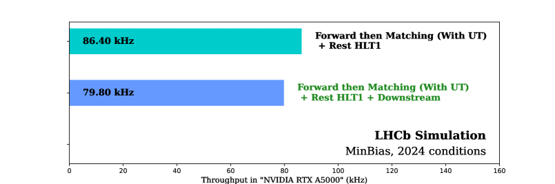
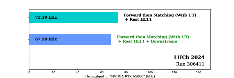
Figure 10: Throughput of the Allen sequence in simulation (top) and data (bottom) including the Downstream algorithm, executed on a RTA A5000 card and compared to other algorithms of the Allen sequence. The rest of the algorithms in the sequence refer to the remaining components of HLT1, which are in charge of the detector decoding, secondary vertex reconstruction, clustering, particle identification, etc…

2.4.2 Momentum resolution

The track momentum resolution is obtained by using several simulated physics samples and is less than 2$\%$. A slight increase is expected in real data due to the non-perfect simulation of the UT detector. Figure 11 shows the momentum resolution for the $\rm{B}^{0}\rightarrow J/\psi K_{s}^{0}$ and $\Lambda_{b}\rightarrow\Lambda\gamma$ decay channels.

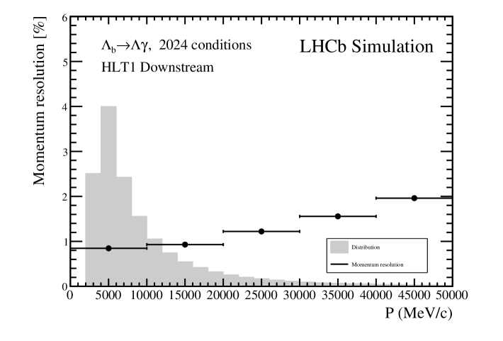
Figure 11: Momentum resolution of the tracks reconstructed by the Downstream algorithm using the simulated $\rm{B}^{0}\rightarrow J/\psi K_{s}^{0}$ decay channel (top) and $\Lambda_{b}\rightarrow\Lambda\gamma$ decay channel (bottom).

2.4.3 Physics efficiency

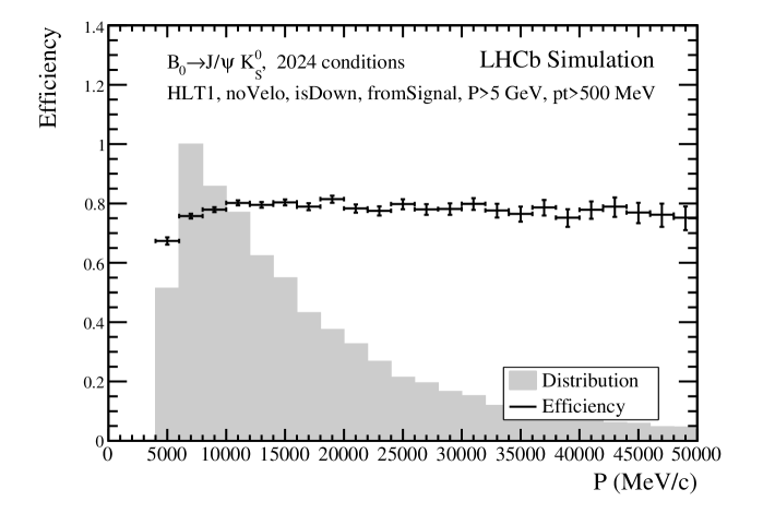
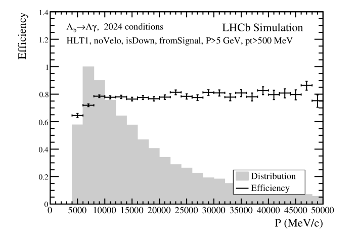
Figure 12: Efficiency of the Downstream algorithm as function of the momentum to reconstruct ${K}^{0}_{\mathrm{\scriptscriptstyle S}}$ from $D^{0}$ decays (top) and $\mathchar 28931\relax$ from $\Lambda_{b}$ decays (bottom). Similar efficiencies are obtained for other decay channels.

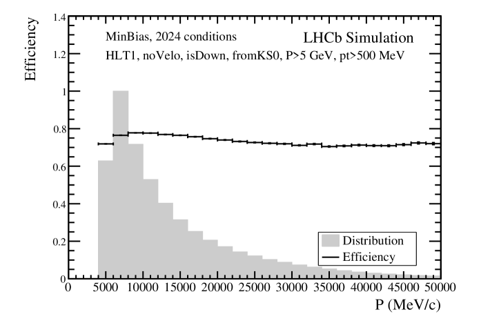
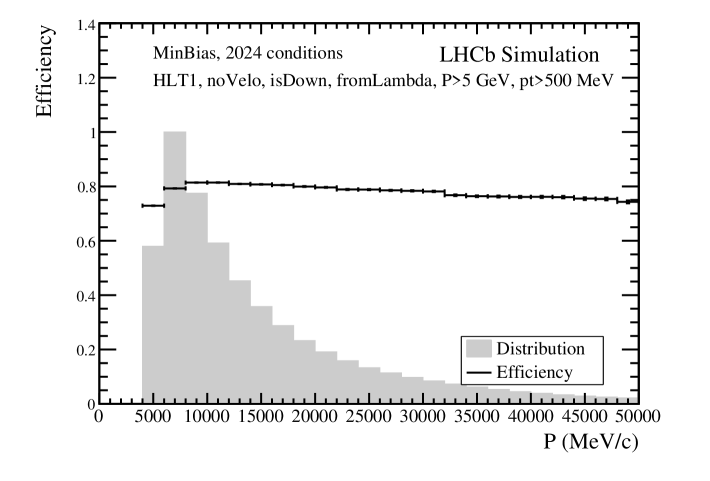
Figure 13: Efficiency of the Downstream algorithm as function of the momentum to reconstruct ${K}^{0}_{\mathrm{\scriptscriptstyle S}}$ (top) and $\mathchar 28931\relax$ (bottom) from minimum bias events.

More than 75$\%$ of the downstream tracks are reconstructed by the algorithm in simulated samples. This has been verified for SM particles ($\mathchar 28931\relax$ and ${K}^{0}_{\mathrm{\scriptscriptstyle S}}$) from different physics decay channels and from minimum bias events, and it is shown in Figs. 12 and 13.

Many new physics models predict long lived particles with masses larger than ${K}^{0}_{\mathrm{\scriptscriptstyle S}}$ and $\mathchar 28931\relax$. During the October 2024 data-taking period, the Downstream algorithm was optimised for SM particles reconstruction, with tolerance windows in the UT tuned using simulated ${K}^{0}_{\mathrm{\scriptscriptstyle S}}$ and $\mathchar 28931\relax$ trajectories to maximise the throughput. If the mass of the particle is much larger, the deflection due to the magnetic field is lower as shown in Fig. 14, and it can escape detection. To increase the algorithm’s efficiency in case of unknown particles, the algorithm has been improved. The strategy has been modified to be able to search for hits in the first and last layers of the UT detector in parallel, without specifying any tolerance window. Special effort is done to keep the same throughput even if the combinatoric is larger, as explained in Sec. 2.1.

The efficiency comparison for the nominal Dv0 version and improved Dv1 is shown in Fig.15, for the SM and new scalar dark bosons of 3 GeV. As one may observe, Dv1 shows similar efficiency in heavy BSM decays as in ${K}^{0}_{\mathrm{\scriptscriptstyle S}}$ and $\mathchar 28931\relax$ decays, overcoming the limitations of Dv0, which is optimized only for ${K}^{0}_{\mathrm{\scriptscriptstyle S}}$ and $\mathchar 28931\relax$ decays. This brings more robustness to our tracking algorithms, removing the dependence with the particle mass. This new configuration will be used during the 2025 data taking period.

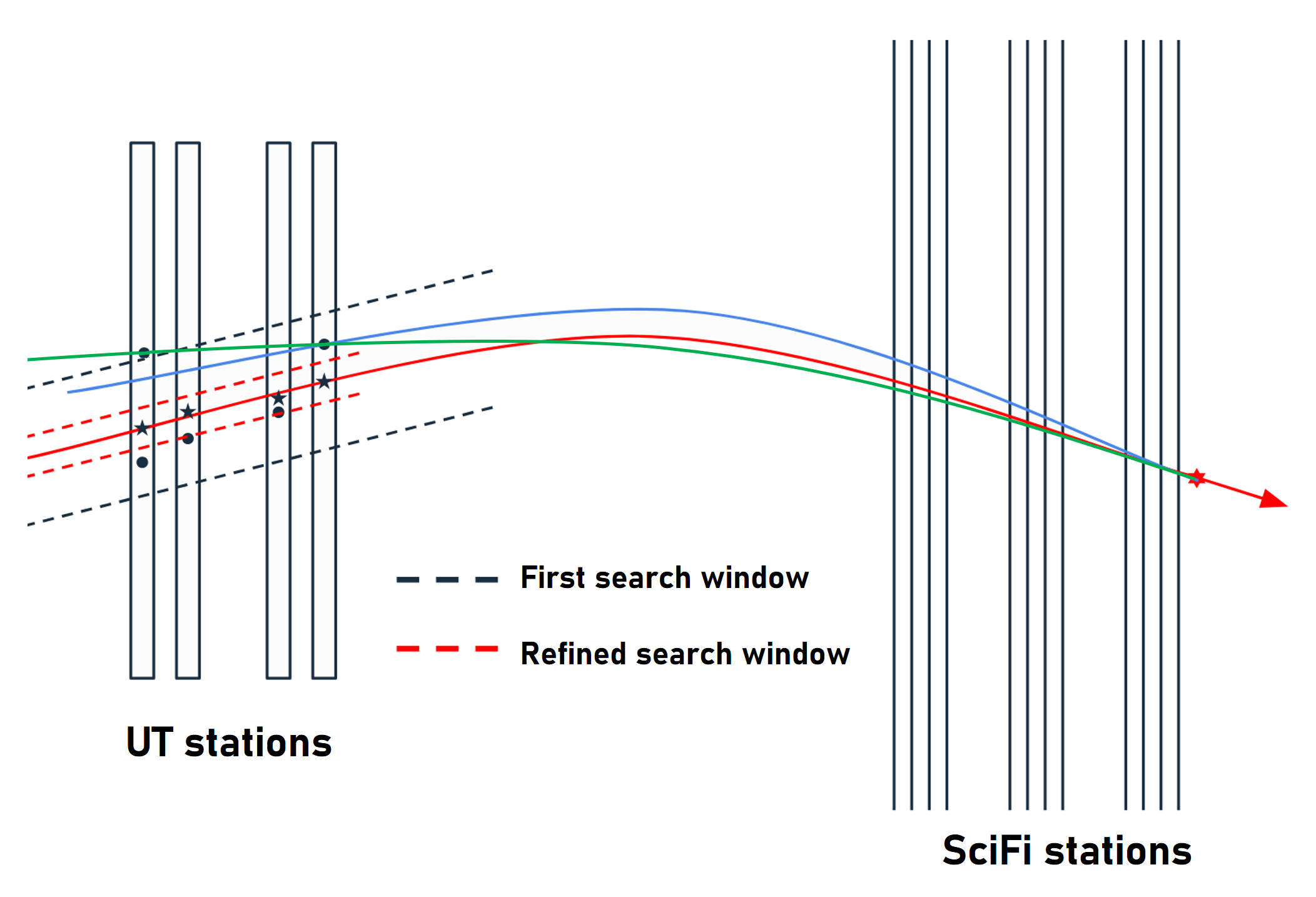
Figure 14: Effect of the search window in the Dv0 of the Downstream algorithm, tuned with ${K}^{0}_{\mathrm{\scriptscriptstyle S}}$ and $\mathchar 28931\relax$ particles, on a new unknown heavier particle (represented in green). The less pronounced curvature can make the search window to be non optimal. This inefficiency has been remedied in the Dv1 of the algorithm.

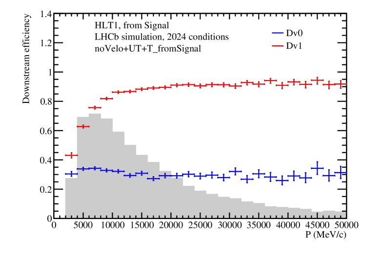
Figure 15: Efficiency comparison of the versions Dv0 and Dv1 of the Downstream algorithm for a new dark boson particle of mass 3 GeV and lifetime of 2 ns.

2.4.4 Ghost rejection

Distributions of the ghost rate vs the momentum are shown in Fig. 16 for two simulated decay channels. The threshold applied to the ghost-killer NN in these figures is 0.5. Lower threshold can give a ghost rate up to 40%, reducing the efficiency of the algorithm.

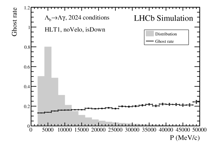
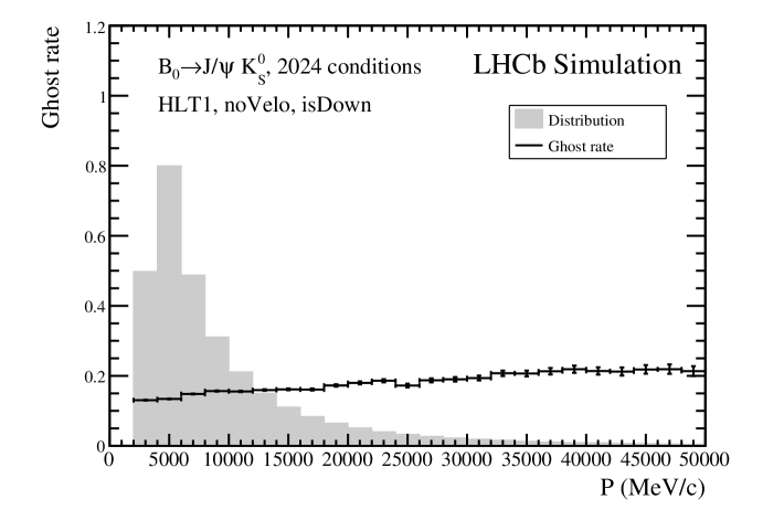
Figure 16: Downstream tracking ghost rate using $\Lambda_{b}\rightarrow\Lambda^{0}\gamma$ (top) and $B_{0}\rightarrow J/\psi K_{S}^{0}$ (bottom) samples, as function of $p$.

2.4.5 Power consumption

The effect on the power consumption from the execution of Downstream algorithm in the HLT1 sequence is studied in the following and shown in Fig. 17. Several techniques are employed to measure the power consumption including the use of a metered power distribution unit (PDU) within the rack, analysis of device driver outputs (e.g., Nvidia DCGM), monitoring CPU performance counters and extracting the estimated power consumption using ACPI system. Consistent results are obtained across all methods.

Only 6% increase in energy consumption is observed due to the highly optimized throughput of the Downstream sequence. The energy consumption of the system is correlated with the throughput, as it can be inferred from Fig. 17.

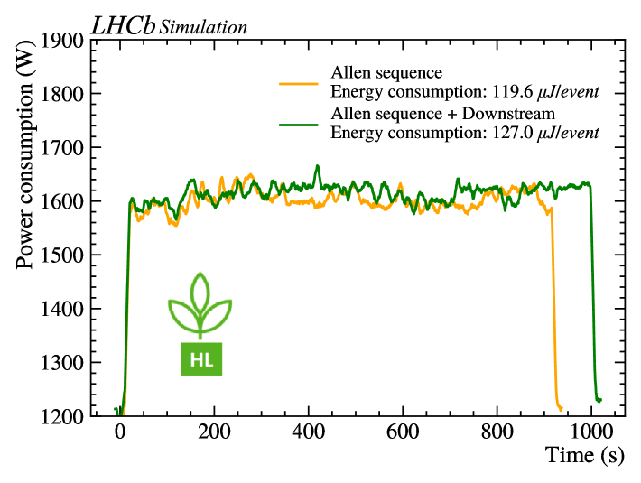
Figure 17: Power consumption with Allen software running over 3.2M $B_{s}\rightarrow\phi\phi$ events without (blue) and with (orange) Downstream algorithm. The power consumption is measured using metered rack PDU AP8858EU3 with an average readout frequency of 2 Hz. The moving average filter with window of 20 points is applied. The measurements are obtained using the NVIDIA RTX 6000 Ada Generation GPU card.

3 Vertexing two downstream tracks

The vertexing of two downstream tracks consists of reconstructing the secondary vertices with two downstream tracks using A Newton-Raphson method and is explained in the following.

The nonzero magnetic field in the $y$ direction between the UT and the vertex position must be taken into account to avoid any bias in the $t_{x}$ slope of the track state at the origin vertex. In HLT1, the downstream track extrapolation cannot use a Runge-Kutta method due to computational costs. Instead, a second-order polynomial for $(z-z_{0})$ is used to determine the $x(z)$ and $y(z)$ coordinates, where $z_{0}$ is the midpoint of the UT station. A parameter in the second-order term ($\gamma$) accounts for the magnetic field. This parameter is obtained by constraining the $t_{x}$ slope at the origin vertex (ovtx):

$$t_{x}(\text{ovtx}_{z})=\left|\frac{dx}{dz}\right|_{z=\text{ovtx}_{z}}=\text{ovtx}_{t_{x}}.$$ (2)

Following simulation studies, the $\gamma$ parameter can be parametrized as function of $q/p$,

$$\gamma(q/p)=-{\cal MP}(-1.5\times 10^{-8}+9.3\times 10^{-3}q/p),$$ (3)

where ${\cal MP}$ corresponds to the magnet polarity. This correction term is applied to the track extrapolation before determining the vertex. The trajectory of each track in $\text{state}_{i}$ given by $(x_{i},y_{i},z_{UT},t_{xi},t_{yi},q/p_{i})$ is thus

$$\text{Traj}_{i}(z) =\matrixquantity[x_{i}+t_{xi}(z-z_{UT})+\gamma_{i}(z-z_{UT})^{2}\\ y_{i}+t_{yi}(z-z_{UT})\\ z]$$ (4)

A Newton-Raphson method Dedieu2015 is applied to find the point of closest approach between two extrapolated tracks, which is then used as the position of the secondary vertex. This method converges quickly, typically finding the solution in three iterations. The bias in the $z$ and $x$ positions of the vertex obtained using this technique are 14 cm and 1 cm, respectively. Figure 18 shows the improvement in the mass distributions for ${K}^{0}_{\mathrm{\scriptscriptstyle S}}$ and $\mathchar 28931\relax$ particles when applying vertex reconstruction to simulated samples. The values are compared with the nominal (PDG) ones.

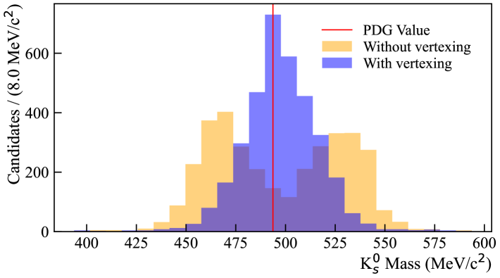
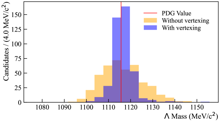
Figure 18: ${K}^{0}_{\mathrm{\scriptscriptstyle S}}$ (top) and $\mathchar 28931\relax$ (bottom) mass distributions before and after applying the vertex reconstruction as explained in the text. Values are compared with nominal (PDG) ones from simulation. The mass resolution after applying the vertex reconstruction is 4 MeV and 15 MeV for ${K}^{0}_{\mathrm{\scriptscriptstyle S}}$ and $\mathchar 28931\relax$ decays respectively.

4 Expected physics impact

Using LHCb simulations with 2024 data-taking conditions, the effect of the Downstream and vertexing algorithms has been studied using several decay channels involving ${K}^{0}_{\mathrm{\scriptscriptstyle S}}$ and $\mathchar 28931\relax$ decays. Two HLT1 trigger lines have been developed to select very detached downstream secondary vertices. The trigger lines rely on four different fast NNs with similar architectures to the one described in Sec. 2.2: one to select ${K}^{0}_{\mathrm{\scriptscriptstyle S}}$ decays, one to select $\mathchar 28931\relax$ decays, one to distinguish detached ${K}^{0}_{\mathrm{\scriptscriptstyle S}}$ decays from prompt ${K}^{0}_{\mathrm{\scriptscriptstyle S}}$ decays, and one to distinguish detached $\mathchar 28931\relax$ decays from prompt $\mathchar 28931\relax$ decays. The inputs to these NNs include track parameters of the two secondary tracks, vertex parameters, and parent track parameters.

These NNs consist of a single hidden layer with 32 nodes and an output layer with a single node. Secondary tracks are required to have opposite charges. A cocktail of simulated physics channels, including detached ${K}^{0}_{\mathrm{\scriptscriptstyle S}}$ and $\mathchar 28931\relax$ particles, is used for the training and testing of the trigger NNs. No overfitting is observed for the model. The NN output provides a classifier score, which determines the signal and background hypothesis of the downstream candidates.

Figure 19 shows the expected increase of efficiency when including triggered downstream tracks at the HLT1 level. The NN threshold for background suppression has been set to 0.5. Some of these channels, such as charm decays decaying into two ${K}^{0}_{\mathrm{\scriptscriptstyle S}}$, or $b$ and charm baryon decays, are only available for downstream tracks, and the efficiency increase is 100$\%$.

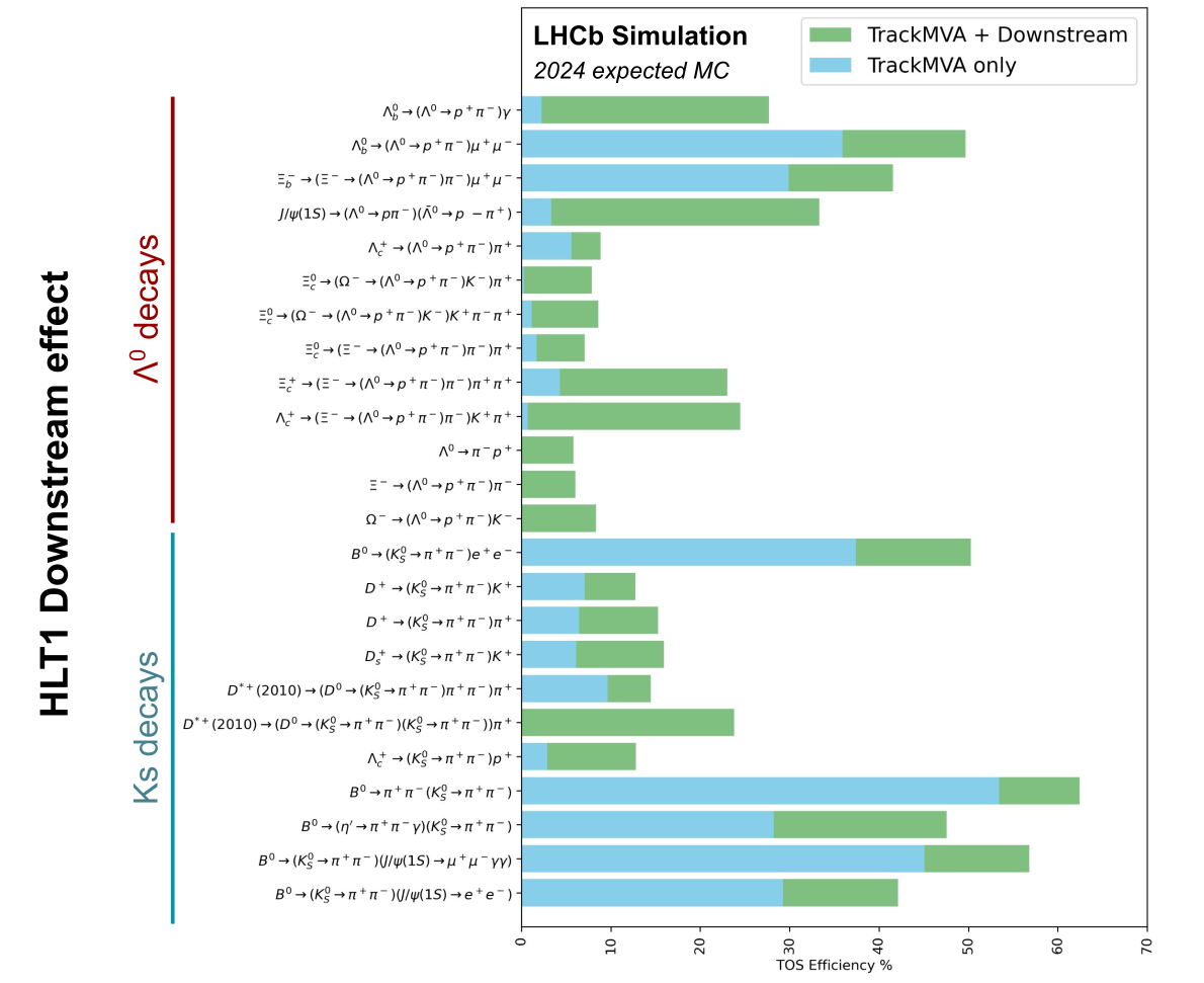
Figure 19: Expected efficiency increase for different triggered ${K}^{0}_{\mathrm{\scriptscriptstyle S}}$ and $\mathchar 28931\relax$ channels due to the inclusion of the Downstream algorithm. The blue band represents the long-track candidates, while the green one adds the selections via downstream tracks.

5 Conclusion

The UT detector has been successfully installed and commissioned during the Summer 2024, providing proper long-tracks reconstruction during the Autumn run. During two weeks in October 2024, and following the installation of 163 additional GPUs, the newly developed Downstream algorithm was included in the full HLT1 sequence.

This algorithm, implemented within the Allen framework at the first level of the LHCb trigger, demonstrates the ability to reconstruct and select highly displaced vertices in real time at a 30 MHz data rate. It achieves high efficiency and low ghost track rates, with significant throughput facilitated by a fast and optimized neural network. Furthermore, its contribution to the overall power consumption of the full Allen sequence has been quantified.

The algorithm’s performance was validated using real data collected in October 2024, successfully reconstructing $\mathchar 28931\relax$ and ${K}^{0}_{\mathrm{\scriptscriptstyle S}}$ particles that do not interact with the VELO detector. This capability is expected to have a high impact on LHCb physics during the 2025 data-taking period. Moreover, a new version of the algorithm extends its applicability to the reconstruction of heavier long-lived particles beyond the Standard Model, opening an unexplored phase-space and offering exciting opportunities for future discoveries Gorkavenko_2024 .

References

- (1) The LHCb Collaboration, J.B.L., et al.: LHCb Upgrade GPU High Level Trigger Technical Design Report. Tech. rep., CERN, Geneva (2020), https://cds.cern.ch/record/2717938
- (2) The LHCb Collaboration, A.: The LHCb Upgrade I. Journal of Instrumentation 19(05), P05065 (May 2024), https://dx.doi.org/10.1088/1748-0221/19/05/P05065
- (3) The LHCb Collaboration, A.: The LHCb Detector at the LHC. Journal of Instrumentation 3(08), S08005 (Aug 2008), https://dx.doi.org/10.1088/1748-0221/3/08/S08005
- (4) The LHCb Collaboration, A.: Long-lived particle reconstruction downstream of the LHCb magnet (2022), https://cds.cern.ch/record/2841793
- (5) Svintozelskyi, V.: Faraway algorithm to reconstruct and trigger vertices from Long-Living Particles at LHCb (2024), https://cds.cern.ch/record/2914251, presented 17 Oct 2024
- (6) Li, P., Rodrigues, E., Stahl, S.: Tracking Definitions and Conventions for Run 3 and Beyond. Tech. rep., CERN, Geneva (2021), https://cds.cern.ch/record/2752971
- (7) The LHCb Collaboration: LHCb Trigger and Online Upgrade Technical Design Report. Tech. rep. (2014), https://cds.cern.ch/record/1701361
- (8) Aaij, R., et al.: Allen: A high-level trigger on GPUs for LHCb. Comput. Softw. Big Sci. 4(1), 7 (2020), https://link.springer.com/article/10.1007/s41781-020-00039-7
- (9) Jashal, B.K.: Triggering new discoveries: Development of advanced HLT1 algorithms for detection of long-lived particles at LHCb (2023), https://cds.cern.ch/record/2881886, presented 07 Nov 2023
- (10) Aiola, S., et al.: Hybrid seeding: A standalone track reconstruction algorithm for scintillating fibre tracker at LHCb. Comput. Phys. Commun. 260, 107713 (2021), https://doi.org/10.1016/j.cpc.2020.107713
- (11) Lederer, J.: Activation Functions in Artificial Neural Networks: A Systematic Overview (2021), https://arxiv.org/abs/2101.09957
- (12) Kingma, D.P., Ba, J.: Adam: A Method for Stochastic Optimization (2017), https://arxiv.org/abs/1412.6980
- (13) Bailly-Reyre, A., Bian, L., Billoir, P., Pérez, D.H.C., Gligorov, V.V., Pisani, F., Quagliani, R., Scarabotto, A., Bruch, D.V.: Looking Forward: A High-Throughput Track Following Algorithm for Parallel Architectures. IEEE Access 12, 114198–114211 (2024), https://doi.org/10.1109/ACCESS.2024.3442573
- (14) Dedieu, J.P.: Newton-Raphson Method. In: Engquist, B. (ed.) Encyclopedia of Applied and Computational Mathematics, pp. 1023–1028. Springer Berlin Heidelberg, Berlin, Heidelberg (2015)
- (15) Gorkavenko, V., Jashal, B.K., Kholoimov, V., Kyselov, Y., Mendoza, D., Ovchynnikov, M., Oyanguren, A., Svintozelskyi, V., Zhuo, J.: LHCb potential to discover long-lived new physics particles with lifetimes above 100 ps. The European Physical Journal C 84(6) (Jun 2024), http://dx.doi.org/10.1140/epjc/s10052-024-12906-3