Test-Time Domain Generalization via Universe Learning: A Multi-Graph Matching Approach for Medical Image Segmentation

Abstract

Despite domain generalization (DG) has significantly addressed the performance degradation of pre-trained models caused by domain shifts, it often falls short in real-world deployment. Test-time adaptation (TTA), which adjusts a learned model using unlabeled test data, presents a promising solution. However, most existing TTA methods struggle to deliver strong performance in medical image segmentation, primarily because they overlook the crucial prior knowledge inherent to medical images. To address this challenge, we incorporate morphological information and propose a framework based on multi-graph matching. Specifically, we introduce learnable universe embeddings that integrate morphological priors during multi-source training, along with novel unsupervised test-time paradigms for domain adaptation. This approach guarantees cycle-consistency in multi-matching while enabling the model to more effectively capture the invariant priors of unseen data, significantly mitigating the effects of domain shifts. Extensive experiments demonstrate that our method outperforms other state-of-the-art approaches on two medical image segmentation benchmarks for both multi-source and single-source domain generalization tasks. The source code is available at https://github.com/Yore0/TTDG-MGM.

1 Introduction

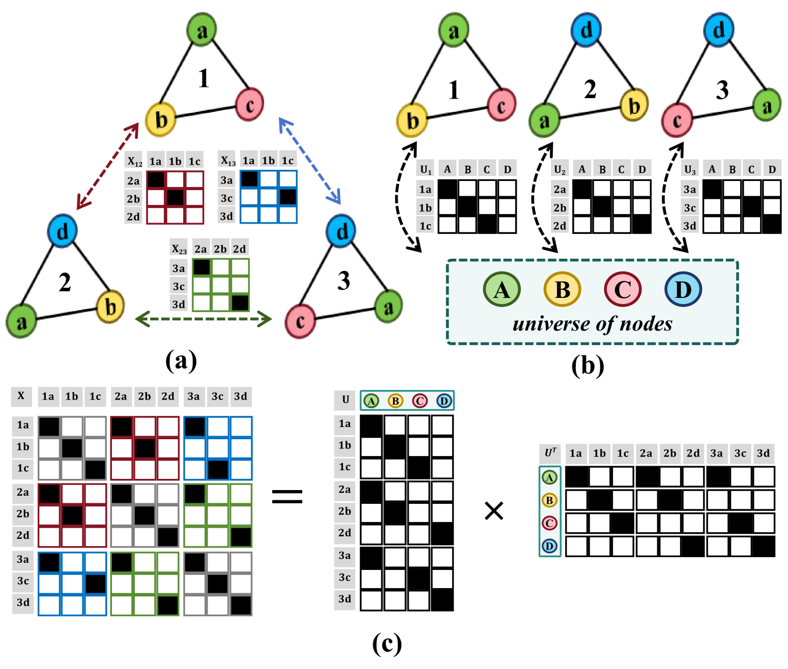
Figure 1: Illustration of multi-graph matching using the universe of nodes. (a) Direct pairwise matching between graphs 1, 2, and 3. (b) Multi-graph matching with the universe of nodes. (c) Equivalence between (a) and (b) (see Lemma 1 in Sec. 2.1 for details).

In the field of medical image processing, semantic segmentation is a technique that enables the precise identification and quantitative analysis of target regions. Currently, a considerable number of medical models can effectively perform segmentation tasks [1, 34]. Nevertheless, when pretrained on source datasets, their performance often declines in real-world deployment due to domain shifts [36, 80] caused by differences in imaging devices, protocols, patient demographics, and preprocessing methods, which impact the model’s generalization ability. To address domain shifts, previous researches in domain adaptation, such as domain generalization (DG) [64, 83, 75], have focused on designing sophisticated models that train jointly on source and target domains or across multiple styled domains. Despite the progress, these methods fall short in practice, as no source domains can fully capture all real-world variations, and retraining for each new data is impractical. Consequently, a more practical approach is to adaptively fine-tune pre-train model using the information from the unlabeled unseen data during the test, which is referred to test-time adaptation (TTA) [31].

Medical images, due to their reliance on specific physical principles (such as X-ray absorption [10], magnetic resonance [59], sound wave reflection [60], etc.), are fundamentally different from images capturing visible light in natural scenes. Moreover, the physiological characteristics of specific anatomical regions exhibit relatively stable shapes and spatial layouts, and the morphology of these structures is predictable [48, 47]. These prior insights provide valuable information that is particularly useful in medical imaging tasks. In areas such as segmentation [74, 33], registration [22], and detection [48, 47], many well-established approaches have been proposed that combine above handcrafted designs with neural network-based methods.

We combine the aforementioned TTA strategies with the prior knowledge of medical images and design a novel Test-Time Domain Generalization (TTDG) framework utilizing graph structures. The construction of graph enables a more robust representation of the morphological priors inherent to medical images. In complex medical scenarios, the aggregation mechanism of nodes and edges in graph ensures the effective preservation of crucial contextual information. Previous research has utilised pairwise graph matching [30, 52, 48] to address domain shifts in medical imaging. However, these methods are limited to aligning features between two domains, which poses challenges in scenarios involving multiple domains commonly encountered in real-world settings. Multi-graph matching overcomes these limitations by establishing connections between multiple graphs and integrating information from diverse domains, thereby enabling the capture of more intricate patterns and structural relationships while maintaining cross-domain consistency. This process facilitates the acquisition of global invariant features from medical images.

In multi-graph matching, the universe of nodes [45, 61] represents the full-set of the nodes from all graphs (refer to Fig. 1). The aforementioned morphological priors are embedded into this universe, derived from a multitude of hospitals, devices, and modalities. It offers three main advantages: (1) Cross-domain consistency. By mapping the nodes from different graphs into the universe, we ensure that all graphs are aligned according to the same reference standard, i.e. the priors. (2) Cycle-consistency in multi-graph matching. This guarantees global coherence across multiple graphs, avoiding conflicts in local node alignments. (3) Handling partial matching and missing nodes. Even when certain nodes are absent in some graphs, matching them to virtual nodes in the universe addresses the issue, enhancing robustness to incomplete graph structures.

Our contributions can be summarized as follows:

• We propose the first (to our best knowledge) multi-graph matching framework for test-time domain generalization in medical image segmentation tasks, effectively mitigating performance degradation caused by domain shifts during the testing phase.

• By designing learnable universe embeddings, we integrate the morphological priors of medical images into the graph matching process during source training, while ensuring the cycle-consistency constraint. This approach enables joint optimization and promotes the learning of domain-invariant features.

• We design a novel, well-initialized unsupervised testing adaptation paradigm that integrates prior knowledge and allows seamless deployment during adaptation, effectively addressing domain shifts.

• We conduct extensive experiments on two typical medical datasets, demonstrating that our method performs competitively against state-of-the-art approaches for both multi-source and single-source domain generalization.

2 Preliminary & Related Work

The following section will introduce the preliminaries of multi-graph matching, while also reviewing the most relevant existing literature on the subject. Subsequently, domain generalization and test-time adaptation will be discussed.

2.1 Multi-Graph Matching

We consider $m\in\mathbb{N}$ different graphs $\mathcal{G}_{1},\mathcal{G}_{2},\cdots,\mathcal{G}_{m}$, $i\in[m]$, $[m]:=\{1,\cdots,m\}$. For each $\mathcal{G}_{i}=(\mathcal{V}_{i},\mathcal{A}_{i})$, $\mathcal{V}_{i}\in\mathbb{R}^{n_{i}\times h}$ represents the $h$-dimensional feature of $n_{i}$ nodes, and adjacency matrix $\mathcal{A}_{i}\in\mathbb{R}^{n_{i}\times n_{i}}$ encodes the connectivity between nodes, represented as the set of edges. For any two graphs $\mathcal{G}_{i}$ and $\mathcal{G}_{j}$, the set of $n_{i}\times n_{j}$ partial permutation matrices $\mathbb{P}_{n_{i}n_{j}}$ is defined as

$$\mathbb{P}_{n_{i}n_{j}}:=\{\mathbb{X}\in\{0,1\}^{n_{i}\times n_{j}}:\mathbb{X}\mathbb{1}_{n_{j}}\leq\mathbb{1}_{n_{i}},\mathbb{X}^{\mathsf{T}}\mathbb{1}_{n_{i}}\leq\mathbb{1}_{n_{j}}\},$$ (1)

where $\mathbb{1}_{n_{i}}$ denotes a $n_{i}$-dimensional column vector whose elements are all ones. The assignment matrix $\mathbb{X}_{ij}\in\mathbb{P}_{n_{i}n_{j}}$ between a pair of graphs $(\mathcal{G}_{i},\mathcal{G}_{j})$ denotes a meaningful correspondence that encodes the matching.

When considering the synchronisation matching [45, 35] of multiple graphs $(m>2)$, relying on local matches between graph pairs can readily result in erroneous correspondences that contradict each other globally [70]. Consequently, the multi-graph matching has been addressed in terms of simultaneously solving under the constraints of cycle-consistency [72, 71].

Definition 1 Cycle-consistency. The matching among $\mathcal{G}_{1},\mathcal{G}_{2},\cdots,\mathcal{G}_{m}$ is cycle-consistent (partial transitivity), if

$$\mathbb{X}_{ik}\mathbb{X}_{kj}\leq\mathbb{X}_{ij},\qquad\forall{i,j,k\in[m]}.$$ (2)

In contrast to full matching, i.e. in Eq. (2) the inequalities become equalities and $n_{i}=n_{j}$, partial matching requires only that the pairwise matching combinations in the cycle form a subset of the identity matching [3]. An iterative refinement strategy [39] was employed to enhance pairwise matchings by ensuring global mapping consistency. In [45], the authors proposed a method to achieve cycle-consistency based on spectral decomposition of the assignment matrix. In addition, methods such as convex programming [7], low-rank matrix recovery [84], and spectral decomposition [35] have been proposed to address the synchronization of partial matchings.

Instead of explicitly modeling the cubic number of non-convex quadratic constraints, a more efficient approach to enforcing cycle consistency is the use of the universe of nodes [61]. In a universe comprising nodes of size $d\in\mathbb{N}$, the matching between graphs can be decomposed by matching each graph $\mathcal{G}_{i}$ to the space of universe (refer to Fig. 1). We denote the universe matchings as follows:

$$\mathbb{U}_{n_{i}d}:=\{\mathbb{U}\in\{0,1\}^{n_{i}\times d}:\mathbb{U}\mathbb{1}_{d}=\mathbb{1}_{n_{i}},\mathbb{U}^{\mathsf{T}}\mathbb{1}_{n_{i}}\leq\mathbb{1}_{d}\}.$$ (3)

Lemma 1 Cycle-consistency, universe matching. The pairwise (partial) matching matrices $\{\mathbb{X}_{ij}\}_{i,j=1}^{m}$ is cycle-consistent iff there exists a collection of universe matching $\{\mathbb{U}_{i}\in\mathbb{U}_{n_{i}d}\}_{i=1}^{m}$, such that for each $\mathbb{X}_{ij}$, it holds that $\mathbb{X}_{ij}=\mathbb{U}_{i}\mathbb{U}_{j}^{\mathsf{T}}$.

The proof will be presented in the appendix. By projecting each node of a graph to the universe of nodes and identifying the universe matchings $\mathbb{U}_{n_{i}d}$, it is ensured that the cycle-consistency constraint will be satisfied throughout the multi-graph matching process. In [66, 68], the authors proposed a gradual assignment procedure to achieve soft matching and clustering through the universe matching. In [4], the universe of nodes is leveraged to incorporate geometric consistency, ensuring both point scaling and convergence. [42] utilized the universe matching to facilitate effective partial multi-graph matching.

Definition 2 Multi-Matching Koopmans-Beckmann’s Quadratic Assignment Problem (KB-QAP) [23]. Multi-graph matching is formulated with KB-QAP, by summing KB-QAP objectives among all pairs of graphs:

$$\underset{\mathbb{X}_{ij}}{\max}\underset{i,j\in[m]}{\sum}( \lambda\cdot\text{tr}(\mathbb{X}_{ij}^{\mathsf{T}}\mathcal{A}_{i}\mathbb{X}_{ij}\mathcal{A}_{j})+\text{tr}(\mathbb{X}_{ij}^{\mathsf{T}}\mathbb{M}_{ij})),$$ (4)

$$s.t.\quad \mathbb{X}_{ij}\in\{0,1\}^{n_{i}\times n_{j}},\mathbb{X}_{ij}\in\mathbb{P}_{n_{i}n_{j}},$$

$$\mathbb{X}_{ik}\mathbb{X}_{kj}\leq\mathbb{X}_{ij},\quad\forall i,j,k\in[m].$$

In Eq. (4), $\lambda$ is a scaling factor for edge-to-edge similarity, and $\mathbb{M}_{ij}$ is the node-to-node similarity between $\mathcal{G}_{i},\mathcal{G}_{j}$.

2.2 Domain Generalization

Domain generalization addresses a challenging scenario where one or more different but related domains are provided, with the objective of training a model that can generalize effectively to an unseen test domain [64, 83, 75]. Medical image analysis encounters significant challenges due to factors such as variability in image appearance, the complexity and high dimensionality of the data, difficulties in data acquisition, and issues related to data organization, labeling, safety, and privacy. Previous research has proposed DG algorithms across multiple levels, including data-level [76, 79], feature-level [5, 28], model-level [17, 46, 86], and analysis-level [33, 49]. Yu et al. [76] proposed a U-Net z-score nomalization network for the stroke lesion segmentation. Liu et al. [33] employed dictionary learning for prostate and fundus segmentation by creating a shape dictionary composed of template masks. In [5], the authors utilized mutual information to differentiate between domain-invariant features and domain-specific ones in ultrasound image segmentation. Gu et al. [17] proposed a domain-style contrastive learning approach that disentangles an image into invariant representations and style codes for DG.

2.3 Test-Time Adaptation

Test-time adaptation is an emerging paradigm that allows a pre-trained model to adapt to unlabeled data during the testing phase, before making predictions [31]. Several TTA methods have been proposed recently, utilizing techniques such as self-supervised learning [6, 24, 81], batch normalization calibration [78, 8, 85, 53, 37], and input data adaptation [55, 21] to achieve better test-time performance. Typically, VPTTA [8] is a method that freezes the pre-trained model and generates low-frequency prompts for each image during inference in medical image segmentation. In [21], the authors proposed designing two CNN-based sub-networks along with an image normalization network. During test-time training, the image normalization network was adapted for each image. [78] proposed a dynamic mixture coefficient and a statistical transformation operation to adaptively merge the training and testing statistics of the normalization layers. Additionally, the authors design an entropy minimization loss to address the issue of domain shifts.

3 Methodology

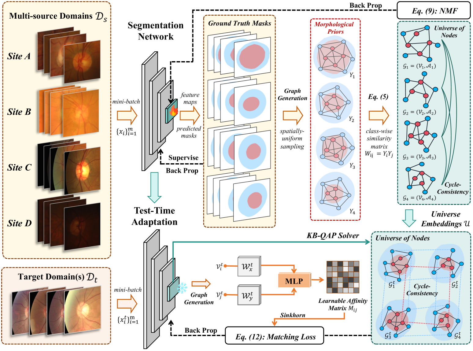
Figure 2: Overview of our TTDG framework. During source model training, data from different domains are jointly used to train the Segmentation Network (feature extractor and segmentation head). Feature maps and ground truth masks are utilized to construct graphs $\mathcal{G}_{i}$ ($i=4$ in this figure legend) and corresponding labels $Y_{i}$ (Sec. 3.1), with universe embeddings learned via back-propagation, incorporating morphological priors (Sec. 3.2). At test time, multi-graph matching is performed on all target domain images in each batch. Despite style differences, these images share common morphological patterns. Universe embeddings are frozen as prior knowledge to guide the matching, and the segmentation network is fine-tuned via back-propagation for efficient adaptation (Sec. 3.3).

This section provides an overview of how multi-graph matching methods can facilitate training for TTDG tasks. Given inputs consisting of images from $S$ source domains $(S\geq 1)$, denoted as $\mathcal{D}_{s}=\{D_{1},D_{2},\cdots,D_{S}\}$, the objective is to enable the model to make more accurate predictions on $T$ unseen target domains $(T\geq 1)$, denoted as $\mathcal{D}_{t}=\{D_{1},D_{2},\cdots,D_{T}\}$, during the testing phase.

Inspired by [47], we aim to effectively leverage morphological prior through graph construction. However, unlike the UDA tasks, which typically involve only two domains, our training process simultaneously handles multiple labeled domains. Pairwise matching across multiple domains can lead to the challenges discussed in Sec. 1. To tackle this, we propose learning domain-invariant latent representations from a multi-graph matching perspective, thereby facilitating rapid adaptation to unseen domains during the TTA phase.

3.1 Construction of Graph

Rather than using conventional graph-matching algorithms that depend on explicitly defined keypoints as graph nodes [15, 65, 67], accurately annotating keypoints in medical imaging is both more costly and less practical than in natural images. Therefore, given a mini-batch $\{x_{i}\}_{i=1}^{m}\in\mathcal{D}_{s}$, as shown in Fig. 2, it is first passed through a general feature extractor, such as ResNet [19], to obtain visual features. We then perform spatially-uniform sampling [29] of pixels within the ground-truth masks at each feature level to obtain $n_{i}$ foreground nodes with its corresponding labels ${Y}_{i}\in\mathbb{Z}^{n_{i}}$. After extracting these fine-grained visual features, we employ a nonlinear projection to transform the visual space into the $h$-dimensional graph space. This approach generates the feature of nodes $\{\mathcal{V}_{i}\in\mathbb{R}^{n_{i}\times h}\}_{i=1}^{m}$ that more effectively preserve the semantic characteristics.

For the weighted adjacency matrix encoding structural information, we use Dropedge [50] to reduce potential bias caused by the frequent visual correspondences, preventing the model from over-relying on specific matches. The formulation is as follows:

$$\mathcal{A}_{i}=Dropedge\{softmax[\mathcal{V}_{i}\mathcal{W}_{x}\cdot(\mathcal{V}_{i}\mathcal{W}_{y})^{\mathsf{T}}]\odot D^{-1}\},$$ (5)

where $\mathcal{W}_{x}$ and $\mathcal{W}_{y}$ are two learnable linear projection, $D=\frac{\mathcal{V}_{i}\mathcal{V}_{i}^{\mathsf{T}}}{||\mathcal{V}_{i}||_{2}}$ is the cosine distance matrix. Edges with larger weights indicate nodes that are closer to each other, so we use the inverse of $D$ and apply the hadamard product $\odot$ to combine node similarity with geometric proximity. The diagonal elements of $\mathcal{A}_{i}$ are set to zero. Based on the above steps, we obtain a corresponding graph $\mathcal{G}_{i}=(\mathcal{V}_{i},\mathcal{A}_{i})$ for each input $x_{i}$.

3.2 Formulation of the Universe Embeddings

In Sec. 2.1, it was demonstrated that by matching each node of a graph to the universe of nodes, we can maintain cycle-consistency while avoiding the computational burden associated with cubic non-convex constraints. While a randomly initialized matrix can learn accurate universe matchings $\mathbb{U}_{n_{i}d}$ in a supervised setting, we introduce universe embeddings $\mathcal{U}\in\mathbb{R}^{d\times h}$, which serve as learnable latent representations to enhance adaptability in unsupervised multi-domain scenarios.

$\mathcal{U}$ is initialized as $1/d+10^{-3}z$, where $z\sim N(0,1)$, following the setting in [66]. For each $\mathcal{G}_{i}$, we learn a unique matching between nodes in $\mathcal{V}_{i}$ and the corresponding in the universe of nodes, as follows: $U_{i}=Sinkhorn(\mathcal{V}_{i}\ \mathcal{U}^{\mathsf{T}},\tau)\in\mathbb{U}_{n_{i}d}$. $Sinkhorn(X,\tau)$ refers to the Sinkhorn algorithm [57, 9], which applies a relaxed projection with entropic regularization [16] to normalize the matrix $X$, resulting in a doubly-stochastic matrix, and $\tau\in(0,+\infty)$ is the regularization factor. For the obtained $U_{i}$, the $d\times d$ matrix $U_{i}^{\mathsf{T}}\mathcal{A}_{i}U_{i}$ is a row and column reordering of $\mathcal{A}_{i}$ based on the universe of nodes. Accordingly, the agreement between two adjacency matrices $\mathcal{A}_{i}$ and $\mathcal{A}_{j}$, reordered according to their respective universe matching assignment matrices $U_{i}$ and $U_{j}$, can be quantified using the Frobenius inner product namely $\langle U_{i}^{\mathsf{T}}\mathcal{A}_{i}U_{i},U_{j}^{\mathsf{T}}\mathcal{A}_{j}U_{j}\rangle$. Let $\mathbb{U}=[U_{1}^{\mathsf{T}},\cdots,U_{m}^{\mathsf{T}}]^{\mathsf{T}}\in\mathbb{R}^{n\times d}$, where $n=\sum_{i=1}^{m}n_{i}$. The block-diagonal multi-adjacency matrix is defined as $\mathbb{A}=diag(\mathcal{A}_{1},\cdots,\mathcal{A}_{m})\in\mathbb{R}^{n\times n}$. We can get the multi-matching formulation as:

$$f(\mathbb{U}):= \ \underset{U_{1},\dots,U_{m}}{\max}\quad\sum_{i,j\in[m]}\langle U_{i}^{\mathsf{T}}\mathcal{A}_{i}U_{i},U_{j}^{\mathsf{T}}\mathcal{A}_{j}U_{j}\rangle$$

$$= \quad\underset{\mathbb{U}\in\mathbb{U}}{\max}\quad\text{tr}(\mathbb{U}^{\mathsf{T}}\mathbb{A}\mathbb{U}\mathbb{U}^{\mathsf{T}}\mathbb{A}\mathbb{U}).$$ (6)

It was observed that in the original multi-graph matching optimization problem, graphs are typically constructed for each individual instance, with all the nodes within a graph belonging to the same category. However, in medical imaging, constructing separate graphs for each organ would not only greatly increase the computational complexity of graph matching but also result in misalignments between graphs from different categories, significantly compromising matching accuracy. To address this limitation, we introduce a class-wise similarity matrix $\mathbb{W}$ to incorporate class-aware label information for each node. This ensures that the nodes are correctly aligned according to their respective categories during multi-graph matching. Specifically, we define $W_{ij}={Y}_{i}{Y}_{j}^{\mathsf{T}}$ and $\mathbb{W}=[W_{ij}]_{ij}\in\mathbb{Z}^{(\sum_{i=1}^{m}n_{i})\times(\sum_{j=1}^{m}n_{j})}$. The class-aware similarity matrix $\mathbb{\tilde{A}}=\mathbb{W}^{\mathsf{T}}\mathbb{A}\mathbb{W}$. Consequently, Eq. (6) can be transformed into the following form

$$\underset{\mathbb{U}\in\mathbb{U}}{\max}\quad\text{tr}(\mathbb{U}^{\mathsf{T}}\mathbb{\tilde{A}}\mathbb{U}\mathbb{U}^{\mathsf{T}}\mathbb{\tilde{A}}\mathbb{U}).$$ (7)

The higher-order projected power iteration (HiPPI) [4] is employed to iteratively solve $\mathbb{U}$ to obtain a stable convergence form:

$$U_{i}^{\ast}=U^{t}_{i}\quad s.t.\quad||U^{t}_{i}-U^{t-1}_{i}||<\theta,\quad\forall i\in[m].$$ (8)

Empirically, we set the convergence threshold $\theta=10^{-5}$. In order to guarantee the optimal learning of universe embeddings $\mathcal{U}$, we incorporate the non-negative matrix factorisation (NMF) [25, 3] and define the overall optimization objective as:

$$L(\mathcal{U})=\sum_{i\in[m]}||{U}^{\ast}_{i}-\mathcal{V}_{i}\ \mathcal{U}^{\mathsf{T}}||^{2}_{F}+\alpha||\mathcal{U}||_{F}^{2},$$ (9)

where $||\cdot||^{2}_{F}$ represents the Frobenius norm, and $\alpha$ is a tuning parameter. Since only matrix multiplication and element-wise division are involved, the Sinkhorn operation is fully differentiable. This allows for effective updates to $\mathcal{U}$ through back-propagation, enabling the incorporation of morphological prior knowledge.

3.3 Testing Paradigm on the Target Domains

During the Test-Time Adaptation (TTA) phase, we only have access to unlabeled data from the unseen target domains $\mathcal{D}_{t}$. Due to distribution shifts, the performance of models trained on $\mathcal{D}_{s}$ can degrade significantly. To address this issue, we employ the multi-graph matching on each mini-batch $\{x_{i}^{t}\}_{i=1}^{m}\in\mathcal{D}_{t}$. By utilizing universe embeddings $\mathcal{U}$ learned from $\mathcal{D}_{s}$ as described in Sec. 3.2, it is guaranteed cycle-consistency, enabling the network to focus on domain-invariant features guided by morphological priors from medical images. In this phase, $\mathcal{U}$ is frozen to prevent error accumulation from affecting the prior information. The feature extractor and segmentation head (segmentation network in Fig. 2) are optimized through gradient back-propagation, allowing the model to adapt effectively to the new domains.

Unsupervised Multi-Matching. Following the same graph construction described in Sec. 3.1, we obtain the $\mathcal{G}_{i}^{t}=(\mathcal{V}_{i}^{t},\mathcal{A}_{i}^{t})$ for each $x_{i}^{t}$, where $\mathcal{V}_{i}^{t}\in\mathbb{R}^{n_{i}\times h}$ represents the $n_{i}$ class-aware nodes and $\mathcal{A}_{i}^{t}\in\mathbb{R}^{n_{i}\times n_{i}}$ is the adjacency matrix encoding the structural information. We first introduce a network-learned affinity matrix $M_{ij}=f_{mlp}\{\mathcal{V}_{i}^{t}\mathcal{W}_{x}^{t}\cdot(\mathcal{V}_{j}^{t}\mathcal{W}_{y}^{t})^{\mathsf{T}}\}\in\mathbb{R}^{n_{i}\times n_{j}}$ in graph pair $\mathcal{G}_{i}$ and $\mathcal{G}_{j}$, which computes the similarity between their corresponding node features. $\mathcal{W}_{x}^{t}$ and $\mathcal{W}_{y}^{t}$ are two learnable linear projection, $f_{mlp}$ is a multi-layer perception (MLP). Subsequently, the matching between $\mathcal{G}_{i}$ and the universe of size $d$ is obtained through the inner-product between $\mathcal{V}_{i}^{t}$ and the pre-trained universe embeddings $\mathcal{U}$, in accordance with the same procedure $U_{i}=Sinkhorn(\mathcal{V}_{i}^{t}\ \mathcal{U}^{\mathsf{T}},\tau)\in\mathbb{U}_{n_{i}d}$ in Sec. 3.2.

In [66, 68], the authors propose solving the multi-matching KB-QAP problem presented in Eq. (4) (denoted as $J$) using a Taylor expansion. Based on the assumptions in Lemma 1 of Sec. 2.1, we can reformulate $J$ in Taylor series as follows:

$$J(U)\approx J(U^{0})+\sum_{i}\frac{\partial J}{\partial U_{i}}\bigg{|}_{U=U^{0}}(U_{i}-U_{i}^{0})+\cdots.$$ (10)

$J$ can be approximated as $m$ linear optimization problems through the first-order Taylor expansion, which can be efficiently solved using the Sinkhorn. The gradient of $J$ with respect to $U_{i}$, denoted as

$$V_{i}=\frac{\partial J}{\partial U_{i}}=\sum_{j\in[m]}(\lambda\mathcal{A}_{i}U_{i}U_{j}^{\mathsf{T}}\mathcal{A}_{j}U_{j}+M_{ij}U_{j}),$$ (11)

$V_{i}$ ensures that $U_{i}$ gradually converges to a high-quality discrete solution.

Finally, the converged $\{U_{i}\}$ fine-tune the segmentation network with the matching loss $L_{mat}$:

$$L_{mat}= \sum_{i,j\in[m]}\left[-\hat{M}_{ij}^{\gamma}(1-U_{i}U_{j}^{\mathsf{T}})\log(U_{i}U_{j}^{\mathsf{T}})\right]$$

$$- \sum_{i,j\in[m]}\left[(1-\hat{M}_{ij})^{\gamma}U_{i}U_{j}^{\mathsf{T}}\log(1-U_{i}U_{j}^{\mathsf{T}})\right],$$ (12)

where $\hat{M}_{ij}=sinkhorn(M_{ij},\tau)$, and $\gamma$ is an amplification factor. See algorithm in appendix for full details.

4 Experiments

4.1 Datasets

The retinal fundus segmentation datasets comprise five public datasets from different medical centers, denoted as Site A (RIM-ONE [14]), B (REFUGE [43]), C (ORIGA [82]), D (REFUGE-Test [43]), and E (Drishti-GS [58]), with 159, 400, 650, 800, and 101 images respectively, all consistently annotated for optic disc (OD) and optic cup (OC) segmentation. We adopted the preprocessing method outlined in [33, 8], where each image’s region of interest is cropped to $800\times 800$ pixels and normalized using min-max normalization.

The polyp segmentation datasets consist of four public datasets collected from different medical centers, denoted as Site A (BKAI-IGH-NEOPolyp [38]), B (CVC-ClinicDB/CVC-612 [2]), C (ETIS [56]), and D (Kvasir [20]), containing 1000, 612, 196, and 1000 images, respectively. We followed the preprocessing steps in [8], resizing the images to $800\times 800$ pixels and normalizing them using ImageNet-derived statistics.

4.2 Experimental Setup

Implementation Details. To ensure a fair comparison across all methods, we followed the protocol in [8] and split each dataset into an $8:2$ ratio for training and testing. We employed the ResNet-50 [19] pre-trained on ImageNet as the feature extractor. The training was optimized using the SGD optimizer with a momentum of 0.9 and a learning rate of 0.001. For source model training, we set the mini-batch size to 8, allowing simultaneous matching of 8 graphs per batch. The universe embedding $\mathcal{U}$ was treated as an additional trainable tensor, integrated into the network weights without influencing subsequent experiments with other methods. During the TTA phase, all methods were trained on the target data without access to their labels. The mini-batch size was set to 4, and the previously learned $\mathcal{U}$ from source model training was frozen. All experiments were implemented using PyTorch and conducted on 4 NVIDIA 3090 GPUs.

Evaluation Metrics. The Dice score (DSC, %) was used to quantify the accuracy of the predicted masks, serving as the primary metric for evaluating segmentation performance. Additionally, the enhanced alignment metric $E_{\phi}^{max}$ [12] was adopted to measure both pixel-level and global-level similarity. To further assess the consistency between predictions and ground truths, we also employed the structural similarity metric $S_{\alpha}$ [11].

4.3 Experimental Results

We selected U-Net [51] as the benchmark model for the segmentation task, training it on the source domains and testing on the target domain without adaptation (No Adapt). In addition, we compared eight state-of-the-art (SOTA) methods, including two entropy-based approaches (TENT [63] and SAR [41]), a shape template-based method (TASD [33]), a dynamically adjusted learning rate method (DLTTA [73]), batch normalization-based methods (DomainAdaptor [78], VPTTA [8]), and noise estimation-based approaches (DeY-Net [69] and NC-TTT [44]).

Table 1: Multi sources domain generaliation in retinal fundus segmentation. The average performance (mean $\pm$ standard deviation) of three trials for our method and nine SOTA methods. “Site A” means training on Sites B-E and testing on Site A, and similarly for the others. The best results are highlighted in red.

3 Methods Site A Site B Site C Site D Site E Average DSC $E_{\phi}^{max}$ $S_{\alpha}$ DSC $E_{\phi}^{max}$ $S_{\alpha}$ DSC $E_{\phi}^{max}$ $S_{\alpha}$ DSC $E_{\phi}^{max}$ $S_{\alpha}$ DSC $E_{\phi}^{max}$ $S_{\alpha}$ DSC $\uparrow$ $E_{\phi}^{max}$ $\uparrow$ $S_{\alpha}$ $\uparrow$ No Adapt (U-Net [51]) 65.60$\pm$5.78 91.75$\pm$0.13 79.11$\pm$0.07 74.65$\pm$4.88 88.78$\pm$0.08 83.31$\pm$0.02 63.15$\pm$7.30 81.03$\pm$0.19 79.77$\pm$0.03 68.11$\pm$5.49 89.46$\pm$0.20 82.12$\pm$0.07 75.34$\pm$1.01 90.68$\pm$0.16 87.53$\pm$0.05 69.37 88.34 82.36 TENT (ICLR’21) [63] 75.22$\pm$3.99 94.10$\pm$0.10 83.97$\pm$0.05 81.06$\pm$0.93 93.45$\pm$0.11 92.36$\pm$0.03 75.23$\pm$2.33 88.10$\pm$0.14 84.62$\pm$0.03 78.12$\pm$2.59 91.33$\pm$0.31 86.41$\pm$0.12 83.17$\pm$0.78 92.74$\pm$0.10 93.64$\pm$0.03 78.56 91.94 88.20 TASD (AAAI’22) [33] 79.70$\pm$2.52 88.73$\pm$0.45 83.67$\pm$0.17 82.96$\pm$2.14 94.01$\pm$0.20 90.99$\pm$0.11 86.12$\pm$1.11 93.59$\pm$0.13 87.08$\pm$0.07 78.02$\pm$6.30 87.20$\pm$0.16 87.94$\pm$0.04 83.71$\pm$3.77 90.88$\pm$0.25 90.37$\pm$0.12 82.10 90.88 88.01 DLTTA (TMI’22) [73] 71.88$\pm$5.59 86.29$\pm$0.21 80.70$\pm$0.13 80.12$\pm$2.26 90.53$\pm$0.17 88.63$\pm$0.06 81.46$\pm$3.35 93.08$\pm$0.08 87.48$\pm$0.02 75.90$\pm$7.27 84.27$\pm$0.12 84.79$\pm$0.06 82.75$\pm$6.55 90.10$\pm$0.31 89.33$\pm$0.14 78.42 88.85 86.18 SAR (ICLR’23) [41] 75.29$\pm$2.69 88.73$\pm$0.34 80.15$\pm$0.26 86.42$\pm$1.57 96.88$\pm$0.27 91.28$\pm$0.09 80.69$\pm$4.30 92.10$\pm$0.15 86.31$\pm$0.27 80.27$\pm$5.47 89.98$\pm$0.31 87.20$\pm$0.15 89.61$\pm$0.28 95.90$\pm$0.08 92.06$\pm$0.01 82.46 92.71 87.40 DomainAdaptor (CVPR’23) [78] 77.14$\pm$1.21 90.80$\pm$0.19 81.31$\pm$0.02 83.95$\pm$0.80 93.17$\pm$0.09 90.44$\pm$0.08 82.79$\pm$1.09 95.36$\pm$0.10 88.57$\pm$0.13 86.50$\pm$3.29 95.26$\pm$0.33 91.07$\pm$0.20 86.24$\pm$1.44 94.90$\pm$0.29 93.77$\pm$0.18 83.32 93.90 89.03 DeY-Net (WACV’24) [69] 79.67$\pm$1.35 89.14$\pm$0.23 83.68$\pm$0.04 90.07$\pm$3.12 97.06$\pm$0.33 92.31$\pm$0.07 85.94$\pm$1.85 93.54$\pm$0.22 87.15$\pm$0.10 83.47$\pm$1.40 95.29$\pm$0.17 88.70$\pm$0.04 88.76$\pm$2.28 95.43$\pm$0.21 90.45$\pm$0.08 85.58 94.09 88.46 VPTTA (CVPR’24) [8] 77.85$\pm$1.40 94.09$\pm$0.01 83.97$\pm$0.05 84.57$\pm$0.99 95.38$\pm$0.03 89.53$\pm$0.09 83.61$\pm$1.67 96.39$\pm$0.04 89.64$\pm$0.05 82.75$\pm$0.50 96.53$\pm$0.04 89.83$\pm$0.01 89.74$\pm$1.51 98.22$\pm$0.24 94.77$\pm$0.07 83.70 96.12 89.55 NC-TTT (CVPR’24) [44] 80.83$\pm$1.77 89.61$\pm$0.23 84.41$\pm$0.08 87.07$\pm$1.31 95.63$\pm$0.06 90.09$\pm$0.02 86.93$\pm$2.27 94.69$\pm$0.11 88.39$\pm$0.03 82.10$\pm$4.28 91.49$\pm$0.22 86.33$\pm$0.07 90.08$\pm$0.99 95.93$\pm$0.10 91.53$\pm$0.09 85.40 93.47 88.15 Ours 82.53$\pm$1.52 91.85$\pm$0.22 85.50$\pm$0.20 88.98$\pm$0.89 96.69$\pm$0.04 91.63$\pm$0.12 88.73$\pm$0.70 95.80$\pm$0.06 89.71$\pm$0.02 90.25$\pm$1.33 97.97$\pm$0.19 92.89$\pm$0.13 91.83 $\pm$0.71 97.14$\pm$0.20 92.82$\pm$0.09 88.46 95.84 90.51 3

Table 2: Multi sources domain generaliation in the polyp segmentation. The average performance (mean $\pm$ standard deviation) of three trials for our method and nine SOTA methods. “Site A” means training on Sites B-D and testing on Site A, and similarly for the others. The best results are highlighted in red.

3 Methods Site A Site B Site C Site D Average DSC $E_{\phi}^{max}$ $S_{\alpha}$ DSC $E_{\phi}^{max}$ $S_{\alpha}$ DSC $E_{\phi}^{max}$ $S_{\alpha}$ DSC $E_{\phi}^{max}$ $S_{\alpha}$ DSC $\uparrow$ $E_{\phi}^{max}$ $\uparrow$ $S_{\alpha}$ $\uparrow$ No Adapt (U-Net [51]) 82.67$\pm$2.24 92.11$\pm$0.07 89.59$\pm$0.10 81.20$\pm$4.38 92.46$\pm$0.20 86.08$\pm$0.06 78.33$\pm$1.62 94.00$\pm$0.08 85.35$\pm$0.01 75.51$\pm$2.74 85.90$\pm$0.17 81.71$\pm$0.21 79.43 91.12 85.68 TENT (ICLR’21) [63] 78.69$\pm$1.12 88.28$\pm$0.14 85.44$\pm$0.08 77.71$\pm$3.09 89.73$\pm$0.09 81.90$\pm$0.12 80.19$\pm$3.35 96.03$\pm$0.04 87.80$\pm$0.17 72.63$\pm$5.11 82.47$\pm$0.30 78.92$\pm$0.14 77.31 89.13 83.52 TASD (AAAI’22) [33] 84.60$\pm$4.14 92.55$\pm$0.21 90.76$\pm$0.10 85.28$\pm$2.20 93.10$\pm$0.13 86.83$\pm$0.19 82.43$\pm$5.39 96.31$\pm$0.08 89.61$\pm$0.02 80.04$\pm$4.41 88.26$\pm$0.11 84.09$\pm$0.03 83.09 92.56 87.82 DLTTA (TMI’22) [73] 80.68$\pm$2.37 90.01$\pm$0.21 86.89$\pm$0.09 80.86$\pm$1.77 91.98$\pm$0.10 85.83$\pm$0.04 75.57$\pm$3.12 93.90$\pm$0.08 84.15$\pm$0.10 74.25$\pm$3.40 83.49$\pm$0.12 79.44$\pm$0.10 77.84 89.85 84.08 SAR (ICLR’23) [41] 79.37$\pm$0.77 88.40$\pm$0.12 86.11$\pm$0.03 78.40$\pm$2.07 90.23$\pm$0.11 83.39$\pm$0.02 80.94$\pm$0.90 95.83$\pm$0.12 86.84$\pm$0.07 78.23$\pm$2.91 86.37$\pm$0.09 81.66$\pm$0.14 79.24 90.21 84.50 DomainAdaptor (CVPR’23) [78] 88.58$\pm$0.96 95.03$\pm$0.04 90.95$\pm$0.01 81.12$\pm$1.07 92.31$\pm$0.08 86.60$\pm$0.02 81.77$\pm$2.17 95.18$\pm$0.03 87.19$\pm$0.01 79.91$\pm$1.33 87.23$\pm$0.04 83.64$\pm$0.05 82.85 92.44 87.10 DeY-Net (WACV’24) [69] 83.61$\pm$2.31 90.79$\pm$0.11 89.25$\pm$0.09 80.90$\pm$3.17 91.49$\pm$0.10 85.36$\pm$0.03 80.46$\pm$1.43 95.83$\pm$0.08 87.14$\pm$0.03 73.85$\pm$3.04 83.00$\pm$0.13 78.96$\pm$0.08 79.71 90.28 85.18 VPTTA (CVPR’24) [8] 82.34$\pm$0.69 91.03$\pm$0.08 88.35$\pm$0.01 84.32$\pm$0.44 91.53$\pm$0.07 87.46$\pm$0.02 84.43$\pm$0.52 95.75$\pm$0.16 88.91$\pm$0.03 82.40$\pm$0.29 89.60$\pm$0.04 85.18$\pm$0.01 83.37 91.97 87.47 NC-TTT (CVPR’24) [44] 87.96$\pm$1.22 93.71$\pm$0.13 90.66$\pm$0.07 83.70$\pm$2.08 93.78$\pm$0.09 87.51$\pm$0.07 89.29$\pm$0.90 96.66$\pm$0.22 91.26$\pm$0.07 78.23$\pm$0.79 86.37$\pm$0.09 81.66$\pm$0.06 84.80 92.63 87.77 Ours 90.97$\pm$0.66 96.57$\pm$0.06 92.92$\pm$0.08 87.49$\pm$0.82 95.21$\pm$0.04 89.93$\pm$0.09 86.87$\pm$0.58 97.53$\pm$0.05 90.16$\pm$0.12 83.97$\pm$1.18 90.67$\pm$0.13 86.44$\pm$0.08 87.32 94.67 89.86 3

Multi-Source Generalization. In these experiments, we adopted a leave-one-out training strategy [6] (i.e., with $S=|\mathcal{D}_{s}\cup\mathcal{D}_{t}|-1$ and $T=1$). Although some methods, such as TASD [33], DeY-Net [69] and VPTTA [8], were originally designed for single-source domain training, we simulated single-domain conditions by mixing multi-source domain data, making the experimental setup still feasible for these approaches. Furthermore, we have also included experiments specifically focused on single-source domains later in the study. The segmentation results for the fundus and polyp datasets are shown in Tables 1 and 2, respectively. For OD/OC segmentation, all TTA methods outperformed the No Adapt baseline, highlighting their effectiveness in addressing domain shifts. Comparatively, our method consistently achieved better average performance than all other approaches. Specifically, for the key segmentation metric DSC, our method exceeded the second-best (DeY-Net [69]) by 2.88% and outperformed the No Adapt by 19.09%. A similar trend was observed in the polyp segmentation results, where we outperformed the second-best method (NC-TTT [44]) and No Adapt by 2.52% and 7.89%, respectively. Additionally, our approach exhibited greater stability across multiple trials compared to the other methods.

Table 3: Single source domain generalization in the polyp segmentation. The average performance of three trials for our method and nine SOTA methods. A $\rightarrow$ B represents models trained on Site A and tested on Site B, and similar for others. Best results are colored as red.

3 Methods A $\rightarrow$ B A $\rightarrow$ C A $\rightarrow$ D B $\rightarrow$ A B $\rightarrow$ C B $\rightarrow$ D C $\rightarrow$ A C $\rightarrow$ B C $\rightarrow$ D D $\rightarrow$ A D $\rightarrow$ B D $\rightarrow$ C Avg. Dice Score Metric $\uparrow$ (DSC, mean$\pm$std ) No Adapt (U-Net [51]) 76.49$\pm$1.48 67.70$\pm$3.27 70.94$\pm$7.56 76.21$\pm$2.90 62.80$\pm$8.03 70.03$\pm$4.53 72.87$\pm$3.62 69.13$\pm$5.15 70.44$\pm$3.27 79.78$\pm$1.08 72.47$\pm$2.80 74.91$\pm$3.18 71.98 TENT (ICLR’21) [63] 68.13$\pm$0.18 65.99$\pm$0.11 66.11$\pm$0.14 77.56$\pm$0.21 59.87$\pm$0.20 68.89$\pm$0.14 73.21$\pm$0.10 65.04$\pm$0.09 72.35$\pm$0.22 77.88$\pm$0.14 70.01$\pm$0.11 73.60$\pm$0.20 69.89 TASD (AAAI’22) [33] 73.02$\pm$2.24 79.67$\pm$6.37 78.23$\pm$4.44 66.82$\pm$9.17 72.09$\pm$4.40 77.95$\pm$1.69 74.20$\pm$3.30 69.74$\pm$7.27 76.13$\pm$2.82 83.77$\pm$0.51 76.09$\pm$3.26 80.10$\pm$1.47 75.65 DLTTA (TMI’22) [73] 72.23$\pm$0.04 70.78$\pm$0.06 74.56$\pm$0.04 64.87$\pm$0.01 60.05$\pm$0.09 78.47$\pm$0.03 71.22$\pm$0.03 65.78$\pm$0.10 71.00$\pm$0.13 79.89$\pm$0.08 79.10$\pm$0.10 74.52$\pm$0.01 71.87 SAR (ICLR’23) [41] 70.34$\pm$0.13 77.90$\pm$0.20 77.71$\pm$0.09 68.19$\pm$0.12 66.56$\pm$0.08 73.92$\pm$0.13 76.12$\pm$0.11 71.29$\pm$0.19 75.08$\pm$0.08 82.07$\pm$0.04 80.44$\pm$0.21 83.10$\pm$0.15 75.22 DomainAdaptor (CVPR’23) [78] 78.39$\pm$0.61 77.09$\pm$0.35 79.45$\pm$0.21 74.98$\pm$0.70 70.07$\pm$0.66 80.21$\pm$0.46 76.02$\pm$0.33 73.40$\pm$0.50 81.33$\pm$0.54 86.10$\pm$0.43 80.56$\pm$0.62 77.86$\pm$0.21 77.96 DeY-Net (WACV’24) [69] 74.45$\pm$1.31 76.07$\pm$2.52 80.11$\pm$0.72 70.90$\pm$1.10 69.23$\pm$2.18 76.31$\pm$1.32 78.33$\pm$4.43 74.60$\pm$1.66 73.52$\pm$2.25 80.70$\pm$0.27 78.23$\pm$1.17 81.48$\pm$0.93 76.16 VPTTA (CVPR’24) [8] 78.18$\pm$0.01 75.14$\pm$0.03 82.73$\pm$0.02 73.65$\pm$0.06 64.78$\pm$0.01 82.86$\pm$0.03 77.90$\pm$0.01 70.64$\pm$0.05 77.22$\pm$0.10 87.19$\pm$0.03 84.97$\pm$0.08 82.12$\pm$0.02 78.12 NC-TTT (CVPR’24) [44] 79.21$\pm$0.24 81.76$\pm$0.57 83.22$\pm$0.69 77.35$\pm$0.33 79.40$\pm$0.67 80.94$\pm$0.54 80.17$\pm$0.70 72.36$\pm$0.62 78.55$\pm$0.43 84.09$\pm$0.38 82.38$\pm$0.51 79.77$\pm$0.74 79.93 Ours 80.47$\pm$0.28 83.93$\pm$0.19 83.18$\pm$0.33 78.33$\pm$0.26 81.25$\pm$0.23 83.58$\pm$0.34 78.86$\pm$0.26 76.49$\pm$0.21 80.20$\pm$0.24 89.17$\pm$0.22 81.68$\pm$0.22 83.86$\pm$0.28 81.75 3

Single-Source Generalization. In these experiments, the models are trained on one domain and tested on the remaining datasets (i.e., with $S=1$ and $T=|\mathcal{D}_{s}\cup\mathcal{D}_{t}|-1$). Compared to multi-source generalization, single-source training is considered more challenging due to the limited domain information available during the training phase. By comparing Tables 2 and 3, we can observe that all models show lower segmentation performance (in terms of DSC) in the single-source setting compared to the multi-source results. Some methods even perform worse than the No Adapt baseline in single-source scenarios. However, our method still achieves the best average performance across 12 domain transfer experiments, outperforming the second-best approach (NC-TTT [44]) by 1.83% and exceeding the No Adapt by 9.77% in terms of DSC.

Fig. 3 presents the visualization results for “Site A” in Table 1. The No Adapt baseline exhibits significant misalignment, with notably distorted shapes and inaccurate boundaries. VPTTA offers some improvement but still suffers from distortions and incomplete segmentation, particularly in the optic cup area. NC-TTT shows instances of overlapping segmentation. In contrast, our method delivers the most precise segmentation, closely aligning with the ground truth. The Grad-CAM [54] visualizations reinforce this, as the attention of network is focused specifically on the relevant regions. These results demonstrate our method’s enhanced generalization to unseen domains by effectively incorporating morphological priors, resulting in higher segmentation accuracy. For further visualization and additional experimental results, please refer to the appendix.

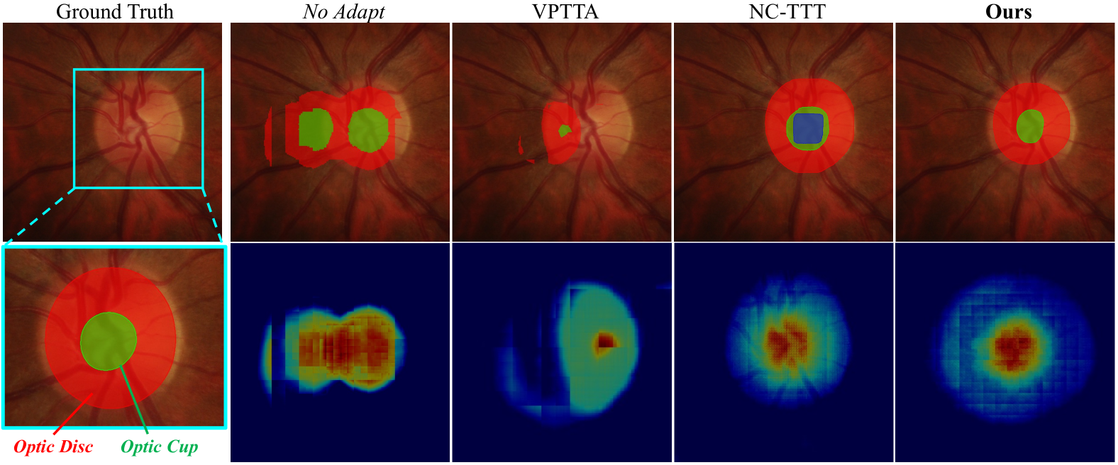
Figure 3: Visualization comparison of segmentation results and Grad-CAM outputs from the final layer of the backbone network for the No Adapt baseline, VPTTA [8], NC-TTT [44], and our proposed method on retinal fundus images. Additional visual comparisons are provided in the supplementary material.

5 Analysis

Table 4: Ablation study in the retinal fundus segmentation. Details of the experiment can be found in Sec 5.1.

3 Methods Site A Site B Site C Site D Site E Average Dice Score Metric $\uparrow$ (DSC, mean$\pm$std ) No Adapt 65.60$\pm$5.78 74.65$\pm$4.88 63.15$\pm$7.30 68.11$\pm$5.49 75.34$\pm$1.01 69.37 w/o $\mathcal{U}$ 77.09$\pm$1.90 83.24$\pm$2.01 80.50$\pm$1.44 78.32$\pm$1.55 83.18$\pm$2.18 80.47 w/o priors 79.51$\pm$0.80 79.36$\pm$1.13 77.40$\pm$1.89 77.29$\pm$1.77 80.00$\pm$1.93 78.71 Ours 82.53$\pm$1.52 88.98$\pm$0.89 88.73$\pm$0.70 90.25$\pm$1.33 91.83$\pm$0.71 88.46 3

5.1 Effectiveness of the Universe Embeddings

The universe embeddings $\mathcal{U}$ play a crucial role in incorporating morphological priors from medical images, resulting in an assignment matrix that projects each node to the universe of nodes. To validate the effectiveness during the TTA, we conducted the following experiments: (1) Without universe embeddings (denoted as w/o $\mathcal{U}$), the universe matching assignment matrix $\mathbb{U}$ is initialized following the setting in [66] (i.e. $\mathbb{U}=1/d+10^{-3}z$, where $z\sim N(0,1)$), leading to random matching between the nodes and the universe; (2) Without morphological priors but with $\mathcal{U}$ (denoted as w/o priors). As shown in Table 4, the performance in (1) is slightly better than in (2) by 1.76% in terms of DSC on average. However, when using the pre-trained $\mathcal{U}$ derived from the source model, the segmentation results show a significant improvement. This highlights the effectiveness of the pre-trained morphological priors embedded in $\mathcal{U}$ for medical imaging tasks.

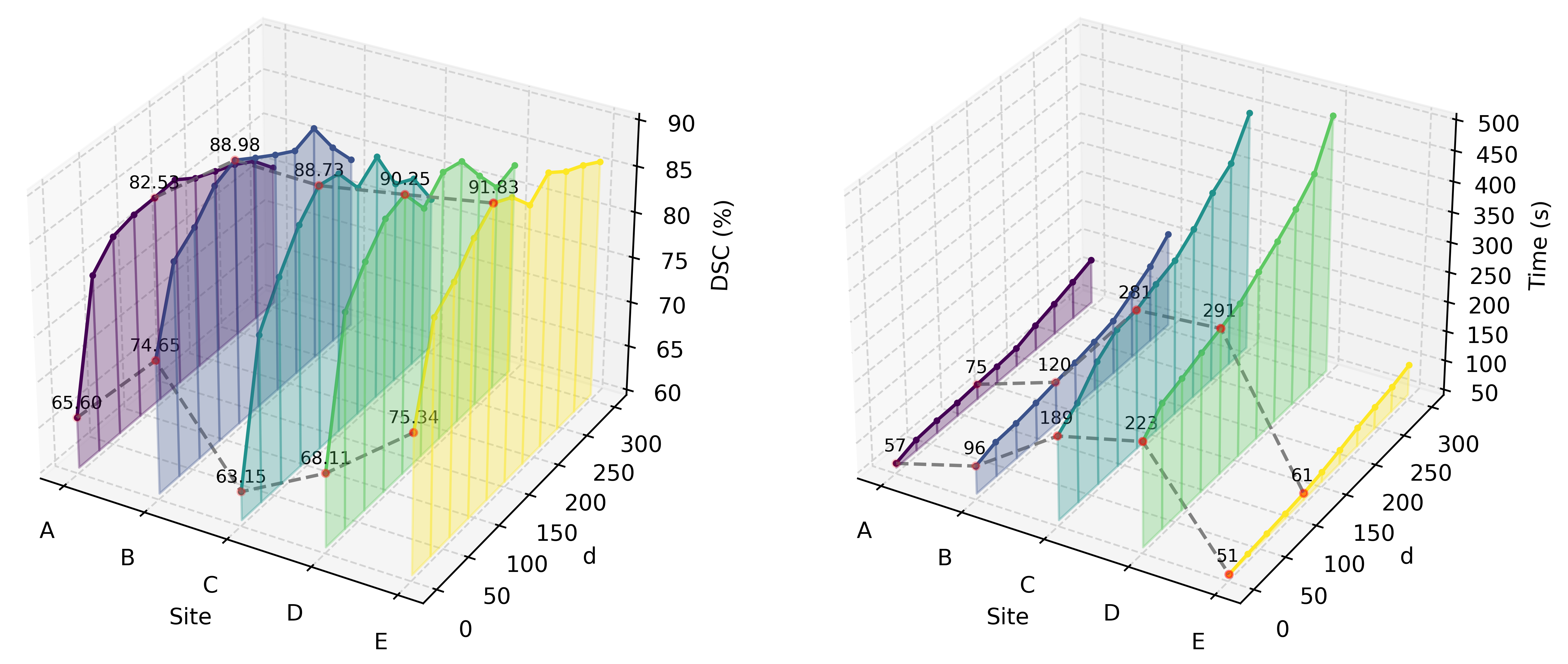
Figure 4: The performance of DSC (%) and inference time (s) with different universe sizes $d$ are shown, with the experimental setup identical to that in Table 1. The first curve represents the No Adapt baseline ($d=0$), while the subsequent curve corresponds to the results obtained with a universe size of $d=120$.

5.2 Effectiveness of the Universe Size

The universe size $d$ directly impacts both the matching accuracy and computational efficiency, and its selection depends on the number of sampled nodes. Previous works [4, 66, 42], ensured that the $d$ matched the number of nodes in each graph by labeling an equal number of keypoints. In our experiments, $d$ is determined by the spatially-uniform sampling described in Sec 3.1, and we empirically set $d=100\times(n+1)s^{-1}$, where $s$ is the sampling step and $n$ is the number of segmentation categories required for the task. We evaluated several $d$, with the results shown in Fig. 4. We observe that excessively small or large step sizes—resulting in too many or too few sampled nodes—negatively impact both training speed and performance. However, when $d$ is within a reasonable range (in this experiment, $s\in[2,10]$ i.e. $d\in[30,150]$.), the model maintains good scalability and performance.

Table 5: Comparison of common variables and performance between pairwise matching and multi-matching, using the same experimental setup as in Table 1. Both methods follow the graph construction in Sec. 3.1.

3 param Site A-E Average description Pairwise [65] Multi-Matching (Ours) lr $10^{-3}$ $10^{-3}$ learning rate batch 4 4 batch size in inference $h$ 256 256 dimension of node feature $\tau$ 0.05 0.05 regularization factor of Sinkhorn Iter 20 20 max iterations of Sinkhorn $d$ - 120 universe size DSC $\uparrow$ 84.63 88.46 dice score metric (%) time $\downarrow$ 0.930 0.392 inference time per image (s/img) Param $\downarrow$ 1.071 0.658 parameter count (M) FLOPs $\downarrow$ 15.35 4.255 floating point operations per second (G) 3

5.3 Multi-Matching vs. Pairwise Matching

Compared to pairwise matching, multi-matching uses cycle-consistency for global optimization, which helps avoid local optima in pairwise. Moreover, joint optimization reduces the computational complexity of large-scale matching. By incorporating morphological consistency constraints, multi-matching exhibits greater robustness. To validate these claims, we conducted experiments comparing the two approaches. For the pairwise matching method, we adopted the benchmark approach [65] and applied the same graph construction process as in multi-matching. The comparison results are presented in Table 5. It is evident that multi-matching outperforms pairwise matching in terms of DSC, inference time, parameters and FLOPs. The inference time of multi-matching was reduced by approximately 57.85% compared to pairwise matching, while segmentation accuracy improved by 3.83% in DSC.

6 Conclusion

This paper presents a novel multi-matching framework for TTDG, which leverages universe embeddings to incorporate morphological priors from medical images while ensuring cycle-consistency, along with an unsupervised test-time paradigm that fully integrates these priors for efficient adaptation. Extensive experiments, including comparisons and ablation studies demonstrate that our graph-matching-based approach achieves SOTA performance, outperforming entropy-based, template-based, batch normalization-based, and noise estimation-based methods across both multi-source and single-source domain generalization tasks.

Supplementary Material

A1 Theoretical Analysis

Lemma 1 (Cycle-consistency, Universe Matching).

Given a set of pairwise (partial) matching matrices $\{\mathbf{X}_{ij}\}_{i,j=1}^{m}$, it is cycle-consistent iff there exists a collection of universe matching matrices $\{U_{i}\in\mathbb{U}_{n_{i},d}\}_{i=1}^{m}$ such that for each graph pair $(\mathcal{G}_{i},\mathcal{G}_{j})$, we have

$$\mathbf{X}_{ij}=U_{i}U_{j}^{\mathsf{T}}.$$

Proof.

We need to prove that the matching matrices $\{\mathbf{X}_{ij}\}_{i,j=1}^{m}$ satisfy cycle-consistency, which means that:

$$\mathbf{X}_{ij}\mathbf{X}_{jk}=\mathbf{X}_{ik}.\forall i,j,k\in[m]$$ (1)

By the assumption of the lemma 1, there exists a collection of universe matching matrices $\{U_{i}\}_{i=1}^{m}$ such that for each pair $(\mathcal{G}_{i},\mathcal{G}_{j})$,

$$\mathbf{X}_{ij}=U_{i}U_{j}^{\mathsf{T}}.$$ (2)

Therefore, we have

$$\mathbf{X}_{ij}=U_{i}U_{j}^{\mathsf{T}},\quad\mathbf{X}_{jk}=U_{j}U_{k}^{\mathsf{T}},\quad\mathbf{X}_{ik}=U_{i}U_{k}^{\mathsf{T}}.$$ (3)

Now we compute $\mathbf{X}_{ij}\mathbf{X}_{jk}$:

$$\mathbf{X}_{ij}\mathbf{X}_{jk} =(U_{i}U_{j}^{\mathsf{T}})(U_{j}U_{k}^{\mathsf{T}})$$

$$=U_{i}(U_{j}^{\mathsf{T}}U_{j})U_{k}^{\mathsf{T}}.$$ (4)

Assume that each matrix $U_{i}$ satisfies $U_{i}^{\mathsf{T}}U_{i}=I$ (i.e., $U_{i}$ is an orthogonal matrix or has unit inner product property). Thus, Eq. (4) simplifies further to:

$$\mathbf{X}_{ij}\mathbf{X}_{jk}=U_{i}IU_{k}^{\mathsf{T}}=U_{i}U_{k}^{\mathsf{T}}=\mathbf{X}_{ik}.$$ (5)

This shows that the matching matrices $\{\mathbf{X}_{ij}\}_{i,j=1}^{m}$ satisfy cycle-consistency. ∎

A2 Algorithm Pipeline

Algorithms 1 and 3 outline the procedures for the source training phase and the test-time adaptation phase, respectively, while Algorithm 2 provides a detailed explanation of the HiPPI [4] method used in Algorithm 1.

A3 Additional Experiments

A1 Single Source DG in Retinal Fundus

Table A1: Single source domain generalization in the retinal fundus segmentation. The performance (mean $\pm$ standard deviation) of three trials for our method and eight SOTA methods. “A $\rightarrow\{B,C,D,E\}$” represents models trained on Site A and tested on the mixed distribution of Sites B-E, and similar for others. Best results are colored as red.

3 Methods A $\rightarrow\{B,C,D,E\}$ B $\rightarrow\{A,C,D,E\}$ C $\rightarrow\{A,B,D,E\}$ D $\rightarrow\{A,B,C,E\}$ E $\rightarrow\{A,B,C,D\}$ Average DSC $E_{\phi}^{max}$ $S_{\alpha}$ DSC $E_{\phi}^{max}$ $S_{\alpha}$ DSC $E_{\phi}^{max}$ $S_{\alpha}$ DSC $E_{\phi}^{max}$ $S_{\alpha}$ DSC $E_{\phi}^{max}$ $S_{\alpha}$ DSC $\uparrow$ $E_{\phi}^{max}$ $\uparrow$ $S_{\alpha}$ $\uparrow$ No Adapt (U-Net [51]) 70.60$\pm$10.01 86.92$\pm$1.17 80.36$\pm$0.88 77.08$\pm$6.90 91.58$\pm$0.84 85.44$\pm$0.99 66.24$\pm$8.45 86.49$\pm$0.77 80.01$\pm$0.91 71.21$\pm$9.47 82.90$\pm$1.48 80.11$\pm$0.88 72.26$\pm$7.60 86.51$\pm$1.02 86.05$\pm$0.68 71.47 86.88 82.39 TASD (AAAI’22) [33] 79.89$\pm$5.91 93.26$\pm$0.21 87.12$\pm$0.13 82.63$\pm$3.24 93.20$\pm$0.25 86.00$\pm$0.10 78.03$\pm$4.29 92.47$\pm$0.14 86.71$\pm$0.09 76.30$\pm$7.81 86.09$\pm$0.15 80.94$\pm$0.11 79.99$\pm$1.29 93.24$\pm$0.10 87.08$\pm$0.08 79.36 91.65 85.57 DLTTA (TMI’22) [73] 74.96$\pm$7.20 89.24$\pm$0.25 84.02$\pm$0.11 78.27$\pm$5.66 92.40$\pm$0.40 85.36$\pm$0.11 75.84$\pm$5.14 90.96$\pm$0.20 84.11$\pm$0.10 65.55$\pm$9.35 84.80$\pm$0.18 78.33$\pm$0.08 71.68$\pm$4.99 87.79$\pm$0.17 85.13$\pm$0.09 73.26 89.03 83.39 SAR (ICLR’23) [41] 74.20$\pm$6.09 89.07$\pm$0.33 83.64$\pm$0.10 80.34$\pm$2.86 92.70$\pm$0.41 85.95$\pm$0.12 72.58$\pm$4.46 91.20$\pm$0.20 83.47$\pm$0.09 70.30$\pm$8.98 85.10$\pm$1.09 79.42$\pm$0.72 70.31$\pm$5.77 88.56$\pm$0.81 86.79$\pm$0.30 73.54 89.32 83.85 DomainAdaptor (CVPR’23) [78] 77.23$\pm$3.97 90.22$\pm$0.40 84.20$\pm$0.11 76.41$\pm$4.28 91.80$\pm$0.31 85.73$\pm$0.12 70.17$\pm$8.01 91.32$\pm$0.24 83.50$\pm$0.09 67.39$\pm$9.82 84.16$\pm$0.21 78.02$\pm$0.08 76.97$\pm$4.59 89.30$\pm$0.13 85.46$\pm$0.08 73.63 89.36 83.38 DeY-Net (WACV’24) [69] 80.03$\pm$8.31 94.42$\pm$0.20 86.35$\pm$0.84 84.30$\pm$7.09 94.25$\pm$0.23 87.16$\pm$0.47 80.32$\pm$7.85 93.40$\pm$0.32 88.41$\pm$0.33 78.67$\pm$5.31 86.12$\pm$0.78 80.45$\pm$0.30 76.81$\pm$3.79 90.09$\pm$0.55 86.30$\pm$0.25 80.02 91.65 85.73 VPTTA (CVPR’24) [8] 73.57$\pm$6.60 92.68$\pm$0.03 84.14$\pm$0.01 78.21$\pm$2.40 94.07$\pm$0.09 86.16$\pm$0.01 69.26$\pm$4.29 92.78$\pm$0.08 82.66$\pm$0.02 60.11$\pm$8.05 85.18$\pm$0.10 76.24$\pm$0.03 72.58$\pm$5.21 91.16$\pm$0.13 84.74$\pm$0.04 70.74 91.17 82.78 NC-TTT (CVPR’24) [44] 78.21$\pm$2.74 93.87$\pm$0.25 85.49$\pm$0.11 82.13$\pm$3.30 93.19$\pm$0.29 86.78$\pm$0.08 77.50$\pm$5.29 91.99$\pm$0.14 84.08$\pm$0.03 74.14$\pm$3.50 87.53$\pm$0.25 80.56$\pm$0.11 80.53$\pm$1.08 92.73$\pm$0.10 85.81$\pm$0.07 78.50 91.86 84.54 Ours 85.25$\pm$2.33 94.68$\pm$0.09 88.52$\pm$0.13 85.34$\pm$3.08 93.18$\pm$0.20 86.83$\pm$0.11 86.19$\pm$1.99 94.57$\pm$0.20 89.24$\pm$0.13 81.52$\pm$4.25 91.20$\pm$0.30 84.53$\pm$0.28 86.08$\pm$3.08 94.60$\pm$0.23 88.58$\pm$0.11 84.87 93.64 87.54 3

For the retinal fundus segmentation task, we conducted single-source domain generalization experiments. Unlike the experiments described in the main text, this setup simulates a more realistic scenario where test data may originate from arbitrarily complex real-world distributions, i.e., mixed distribution shifts. Specifically, data from one site was selected and split $8:2$ into training and validation sets ($S=1$), while the remaining sites ($T=|\mathcal{D}_{s}\cup\mathcal{D}_{t}|-1$) were shuffled and used entirely as the testing dataset. Notably, all models encountered these target domains for the first time during testing.

As shown in Table A1, our approach achieved SOTA performance across all five transfer experiments for the DSC metric. In the average results, we outperformed the second-best method (DeY-Net [69]) by 4.85%, 1.78%, and 1.81% in the DSC, $E_{\phi}^{max}$, and $S_{\alpha}$, respectively. These results validate the effectiveness of our method for medical image segmentation tasks.

The retinal fundus dataset is characterized by significant low-level visual differences and features segmentation targets that are not singular, often exhibiting overlapping and fixed structures. We attribute our superior performance to the comprehensive learning of the morphological knowledge of organs. This enables our method to robustly distinguish organ instances and their shape features—a domain-invariant property—even under severe domain shifts that degrade the performance of other methods.

A2 Multi Source DG in MRI Prostate

Datasets. We conducted experiments on the prostate segmentation task using T2-weighted MRI scans collected from six different clinical centers, denoted as Domain RUNMC, BMC, I2CVB, UCL, BIDMC, and HK. These centers are sourced from three publicly available datasets: NCI-ISBI13 [40], I2CVB [26], and PROMISE12 [32].

Implementation Details. We followed the data preprocessing pipeline of [77] to ensure consistency. Specifically, we used 30 labeled cases from RUNMC as the source dataset and evaluated the model on 30, 19, 13, 12, and 12 unlabeled cases from the five remaining clinical sites. Each MRI axial slice was resized to $384\times 384$ pixels and normalized to have zero mean and unit variance. Before normalization, we clipped the 5%–95% intensity range of the histograms to reduce outlier influence.

For feature extraction, we employed a ResNet-50 backbone pre-trained on ImageNet. During both the source model training and test-time adaptation (TTA) stages, we maintained a batch size of 8. Given that edge precision is crucial in MRI prostate segmentation, and considering the complex shape variations of the prostate, we selected Dice Score (DSC) and Hausdorff Distance (HD95) as the primary evaluation metrics to provide a comprehensive performance assessment.

Experimental Results.

Table A2: Test-time domain generalization results on the MRI prostate datasets. The performance (mean $\pm$ standard deviation) of three trials for our method and six SOTA methods. Best results are colored as red.

3 Methods BMC I2CVB UCL BIDMC HK Avg. DSC HD95 DSC HD95 DSC HD95 DSC HD95 DSC HD95 DSC $\uparrow$ HD95 $\downarrow$ No Adapt 74.30$\pm$5.31 16.08$\pm$12.41 66.47$\pm$13.50 37.16$\pm$18.24 75.28$\pm$6.20 16.77$\pm$12.10 52.08$\pm$7.71 50.09$\pm$20.85 80.51$\pm$9.35 8.79$\pm$9.06 69.72$\pm$8.29 25.77$\pm$15.41 TENT (ICLR’21) [63] 77.45$\pm$3.79 12.09$\pm$9.88 69.10$\pm$10.47 30.78$\pm$19.22 79.69$\pm$4.81 14.71$\pm$11.01 52.01$\pm$6.80 42.63$\pm$10.13 84.58$\pm$2.73 4.07$\pm$5.38 72.56$\pm$4.26 20.85$\pm$13.64 TASD (AAAI’22) [33] 76.28$\pm$2.35 15.11$\pm$15.17 68.30$\pm$7.88 31.43$\pm$24.10 80.25$\pm$3.54 10.59$\pm$16.39 56.08$\pm$3.82 51.90$\pm$24.82 81.09$\pm$1.79 4.26$\pm$4.16 72.40$\pm$5.72 22.65$\pm$17.53 SAR (ICLR’23) [41] 77.24$\pm$4.26 20.48$\pm$10.12 68.99$\pm$8.27 49.07$\pm$15.66 79.27$\pm$8.48 18.03$\pm$5.89 50.81$\pm$10.60 54.35$\pm$19.31 85.40$\pm$3.08 3.87$\pm$3.55 72.34$\pm$4.80 29.16$\pm$16.28 DomainAdaptor (CVPR’23) [78] 76.49$\pm$2.59 19.27$\pm$8.13 69.07$\pm$9.14 32.57$\pm$10.40 80.41$\pm$5.08 16.24$\pm$9.88 49.99$\pm$14.28 48.40$\pm$10.28 85.20$\pm$1.90 3.25$\pm$6.94 72.23$\pm$6.82 23.94$\pm$14.55 VPTTA (CVPR’24) [8] 77.42$\pm$4.38 12.93$\pm$7.09 70.25$\pm$5.18 30.01$\pm$13.68 82.07$\pm$6.27 13.28$\pm$18.09 57.49$\pm$8.46 40.11$\pm$12.05 83.27$\pm$2.96 3.40$\pm$5.45 74.10$\pm$4.79 19.94$\pm$12.99 PASS (TMI’24) [77] 80.07$\pm$7.14 10.50$\pm$9.57 71.41$\pm$6.28 28.26$\pm$9.97 84.39$\pm$8.81 10.68$\pm$12.27 57.27$\pm$11.48 36.94$\pm$16.43 84.88$\pm$3.71 3.03$\pm$5.05 75.60$\pm$5.13 17.88$\pm$12.14 Ours 79.63$\pm$4.71 9.99$\pm$11.10 74.09$\pm$9.80 25.70$\pm$13.07 86.30$\pm$7.25 11.08$\pm$17.47 60.33$\pm$13.59 39.52$\pm$14.20 86.12$\pm$2.08 2.84$\pm$8.08 77.29$\pm$3.98 17.82$\pm$11.06 3

The MRI prostate segmentation results are presented in Table A2, where we compare our method against several SOTA approaches, including the latest TTA segmentation method, PASS [77]. As shown in the results, the performance of existing TTA methods remains relatively close across both DSC and HD95 metrics. While PASS exhibits strong segmentation performance, our method surpasses it with a 1.69% improvement in DSC, demonstrating its effectiveness. Given the inherent challenges of MRI prostate segmentation, characterized by diverse imaging modalities and complex morphological variations, our results highlight the robust generalization capability of our approach. Nonetheless, further enhancing edge precision remains an important focus for our future work.

A3 Natural Image Classification

Datasets. For natural image classification tasks, we selected two benchmark datasets: PACS [27] and VLCS [13], which are widely used in domain generalization and test-time adaptation studies. The PACS [27] dataset consists of large images spanning 7 classes evenly distributed across 4 domains, i.e. A (Art), C (Cartoons), P (Photos), and S (Sketches), with a total of 9,991 images. The VLCS [13] dataset comprises 10,729 images across 5 classes (bird, car, chair, dog, and person), evenly distributed across 4 domains: C (Caltech101), L (LabelMe), S (SUN09), and V (VOC2007).

Source model training. For all experiments, we employed an ImageNet-pretrained ResNet-50 [19] as the feature extractor, with an MLP layer provided by the DomainBed [18] benchmark serving as the classifier. We used the SGD optimizer with a learning rate of $1\times 10^{-5}$. The batch size was set to 32, and training was conducted for 10,000 iterations. All images were resized to $224\times 224$, and data augmentation techniques—including random cropping, flipping, color jittering, and intensity adjustments—were applied during source training.

Implementation details of test-time adaptation setup. We evaluated our framework against six methods (i.e. Empirical Risk Minimization (ERM) [62], DomainAdaptor [78], ITTA [6], VPTTA [8], NC-TTT [44]) under fair comparison conditions, following the leave-one-out training strategy using the publicly available DomainBed [18] framework. For deploying our framework at the test-time phase, we employed SGD with a learning rate of 0.005, a batch size of 16, and a universe size of $d=60$. Notably, as all images in the natural image classification task contain only a single instance class, the class-wise similarity matrix described in Section 3.2 of the main text was not utilized.

Experimental Results. The classification results across different domains for natural images are presented in Tables A3 and A4. While the ERM method shows strong performance compared to existing approaches, our method achieves higher classification accuracy, surpassing ERM by 3.01% on the PACS dataset and 2.49% on the VLCS dataset. Additionally, our approach demonstrates competitive performance against state-of-the-art test-time adaptation methods designed for natural images. Natural images present greater challenges compared to medical images due to the lack of consistent morphological priors typically observed in the latter. However, unlike segmentation tasks, classification does not require determining the specific class of every pixel in an image. Our framework’s graph construction effectively captures spatial correspondences for each instance, further enhancing its performance.

Table A3: Test-time domain generalization results on the PACS [27] dataset using a ResNet-50 backbone. Each column (A, C, P, S) indicates the domain used as the test set, while the remaining domains are used for training. The best results are highlighted in red.

3 Method A C P S Avg. ERM [62] 84.07 80.21 97.06 81.99 85.83 TENT (ICLR’21) [63] 82.34 78.63 97.93 82.72 85.40 DomainAdaptor (CVPR’23) [78] 86.15 82.02 98.40 84.38 88.45 ITTA (CVPR’23) [6] 85.63 84.30 97.27 84.09 87.82 VPTTA (CVPR’24) [8] 86.50 83.77 97.09 85.10 88.12 NC-TTT (CVPR’24) [44] 83.81 80.44 96.53 82.36 85.79 Ours 85.08 83.93 98.61 87.76 88.84 3

Table A4: Test-time domain generalization results on the VLCS [13] dataset using a ResNet-50 backbone. Each column (C, L, S, V) indicates the domain used as the test set, while the remaining domains are used for training. The best results are highlighted in red.

3 Method C L S V Avg. ERM [62] 97.63 64.20 70.39 74.41 76.66 TENT (ICLR’21) [63] 96.88 64.46 71.07 73.52 76.48 DomainAdaptor (CVPR’23) [78] 98.69 69.18 73.66 76.01 79.39 ITTA (CVPR’23) [6] 97.30 66.09 72.31 75.10 77.70 VPTTA (CVPR’24) [8] 97.25 67.69 71.78 75.22 77.98 NC-TTT (CVPR’24) [44] 96.72 65.58 73.04 76.83 78.04 Ours 98.49 68.72 74.12 75.30 79.15 3

A4 Additional Visualization

We conducted additional visualization experiments, with segmentation results for retinal fundus and polyp images shown in Figures A1 and A2, respectively. Each row represents images from a distinct domain (Site), and we ensured that the model performing inference had not encountered images from that domain before.

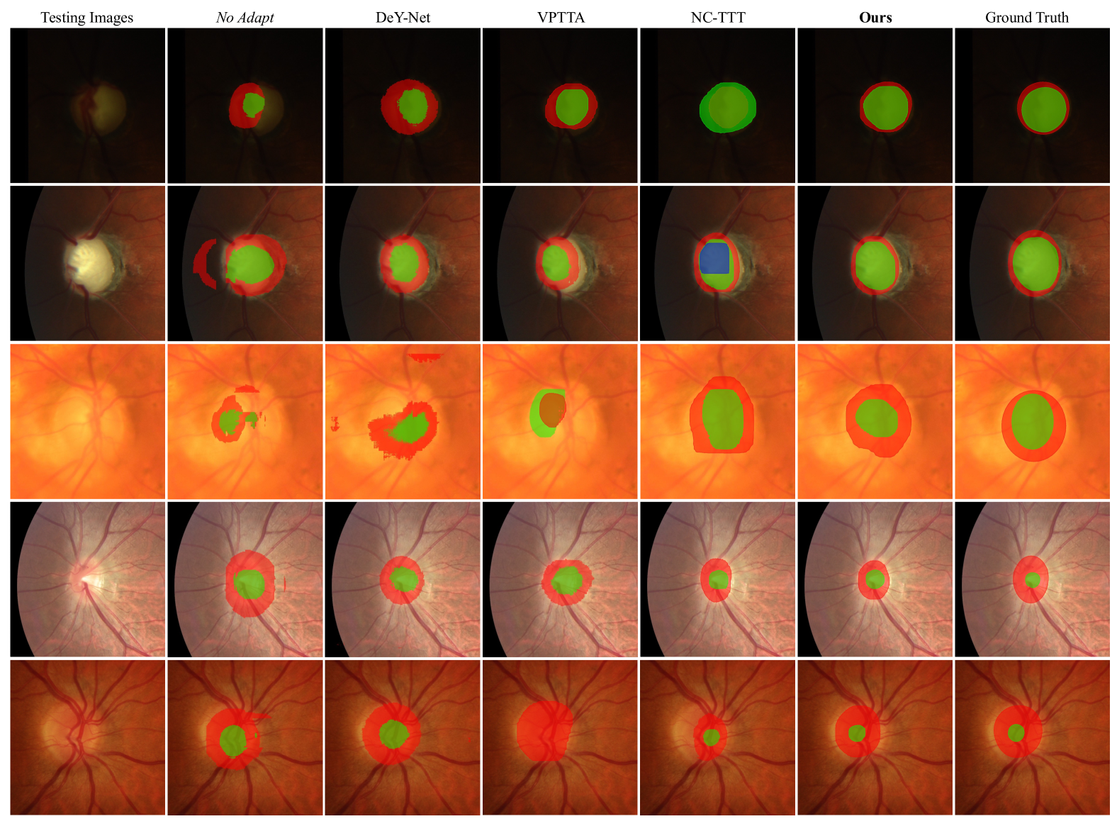
Figure A1: Visualization comparison of segmentation results for the No Adapt baseline, DeY-Net [69], VPTTA [8], NC-TTT [44], and our method in retinal fundus segmentation. The five rows from top to bottom display the final segmentation results for tests conducted on Sites A to E. Different colors represent the segmentation instances of different classes identified by the network.

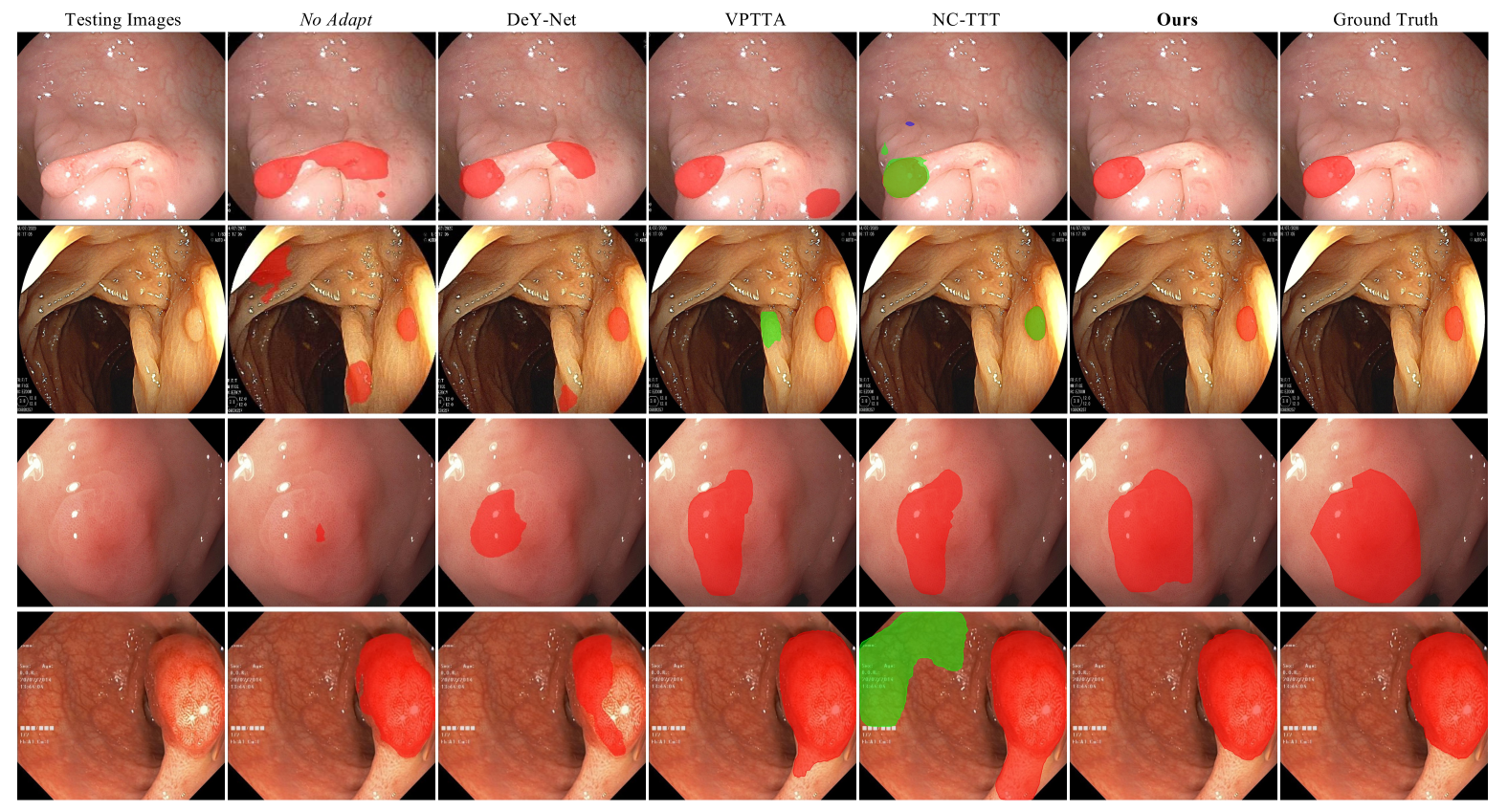
Figure A2: Visualization comparison of segmentation results for the No Adapt baseline, DeY-Net [69], VPTTA [8], NC-TTT [44], and our method in polyp segmentation. The four rows from top to bottom display the final segmentation results for tests conducted on Sites A to D. Different colors represent the segmentation instances of different classes identified by the network.

Retinal fundus segmentation, in particular, presents a challenge due to the presence of two overlapping substructures. Lower clarity and contrast in images (e.g., rows 1 and 2 of Figure A1) further complicate the model’s ability to accurately differentiate and segment these structures. By incorporating morphological priors of the organ within a multi-graph matching network, our method effectively learns robust substructure representations while minimizing domain-related noise. This approach overcomes issues like repeated, missing, or blurred edge pixels commonly seen in other methods, providing a more precise segmentation outcome.

The segmentation of polyps presents a greater challenge than that of retinal fundus imaging due to the highly variable appearance, with marked differences in shape, size, and color across domains. This variability demands precise, pixel-level classification from the network. Furthermore, we have not designated polyp segmentation as a single-object task; the model independently classifies and segments multiple classes during testing, using different colors to distinguish each segmented object in the visualization. As illustrated in Figure A2, the masks generated by our method are in close alignment with expert annotations and effectively avoid pixel misclassification into different categories, a common issue in other methods.

A4 Additional Analysis

A1 Effectiveness of the class-wise similarity matrix

The class-wise similarity matrix $\mathbb{W}$ is introduced to mitigate category confusion in graphs caused by nodes belonging to different classes. Such confusion often results in mismatches, semantic deviations, and redundant computations. By reordering the adjacency matrix based on the labels $Y_{i}$ of each node $\mathcal{V}_{i}$, our method strengthens the capacity to identify and learn class-specific information during the source training phase. To validate the above perspective, we conducted experiments comparing the final TTA segmentation results with and without $\mathbb{W}$ (denoted as with $\mathbb{W}$ and w/o $\mathbb{W}$). As illustrated in Figure A4, w/o $\mathbb{W}$ results in a measurable decline in DSC performance. Furthermore, we visualized the effect of w/o $\mathbb{W}$ in multi-object segmentation scenarios, as shown in Figure A5. While the masks generated by the model closely align with the ground truth, the model misclassified the categories of two segmented instances.

A2 Effectiveness of Morphological Priors

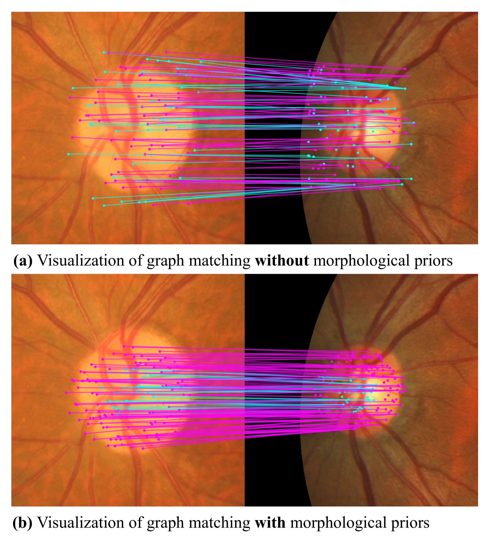
Figure A3: Visualization of graph pair matching.

We visualized cross-site pairing without morphological priors, as shown in Fig.  A3(a), and compared it with the results obtained after incorporating priors, as shown in Fig.  A3(b). Without priors, the graph nodes were not correctly sampled within the corresponding organs, leading to mismatches. By introducing priors, this issue was effectively resolved, and multigraph matching ensured more stable pairing across multiple domains. For a quantitative evaluation of the impact of without priors, please refer to Table 4 in the main text.

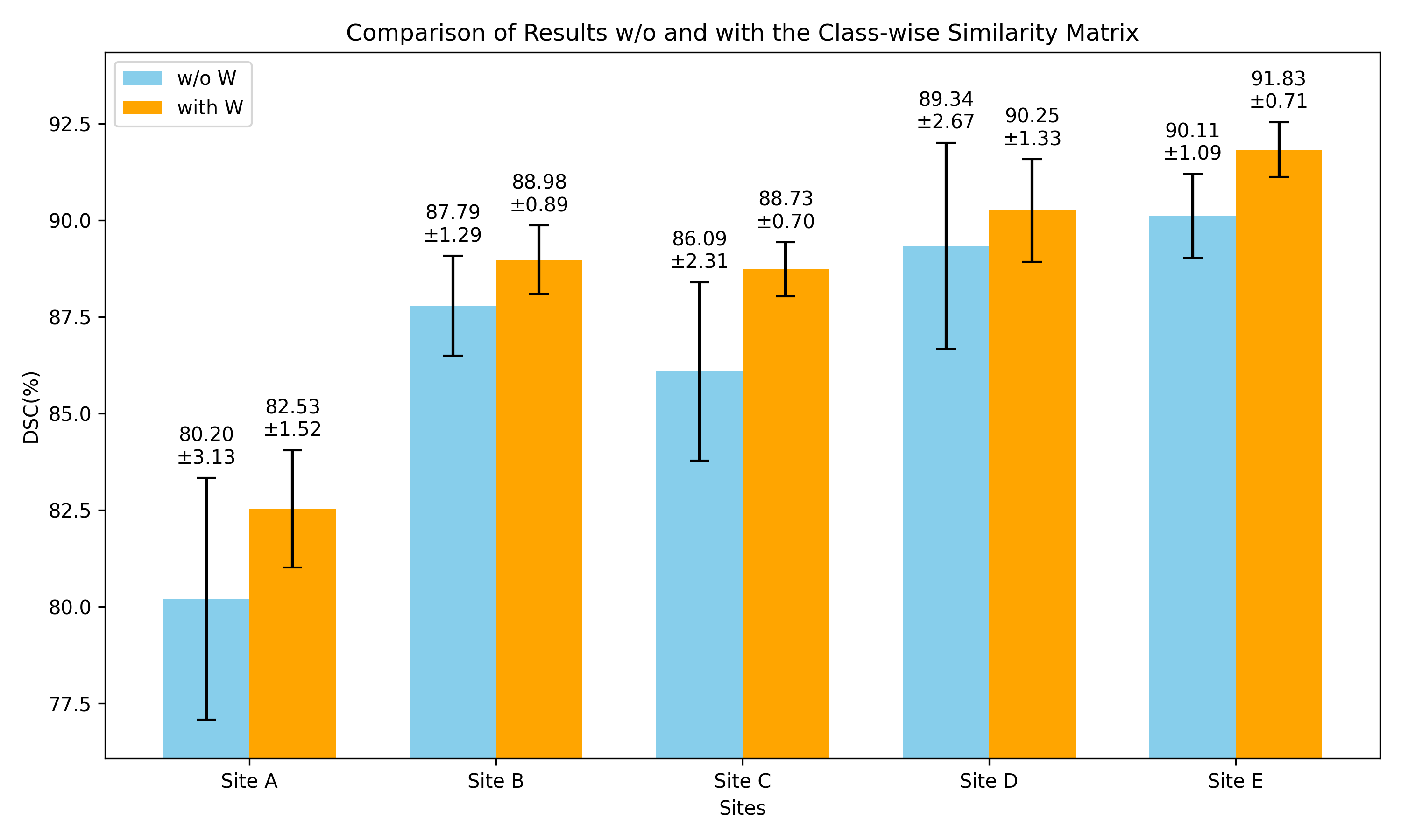
Figure A4: Ablation study on the impact of the Class-wise Similarity Matrix $\mathbb{W}$ in retinal fundus segmentation: comparison of results with and without (w/o) $\mathbb{W}$.

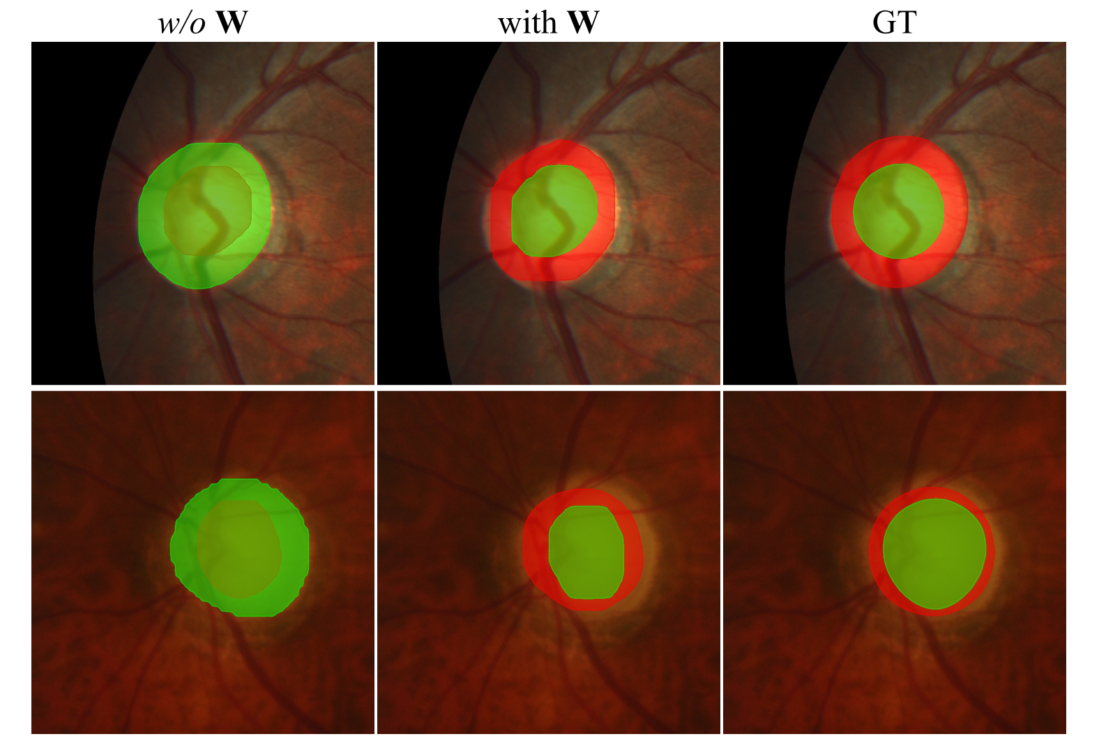
Figure A5: Visualization of segmentation results with and without (w/o) the Class-wise Similarity Matrix $\mathbb{W}$.

A3 Impact of Batch Size on Segmentation

Table A5: Ablation study on batch size during TTA for retinal fundus segmentation. “Avg. DSC” represents the average DSC across the five sites, while “time” indicates the inference time per image.

3 Batch Size Avg. DSC FLOPs (G) time (s/img) 2 85.20 3.012 0.277 4 88.46 4.255 0.392 8 88.93 20.43 0.780 16 89.15 80.96 1.831 32 88.31 223.1 3.715 3

As shown in Table A5, increasing the number of simultaneously matched graphs leads to a significant increase in both FLOPs and inference time, while the improvement in segmentation quality remains marginal. To achieve a balance between segmentation performance and computational efficiency, we set the mini-batch size to 4 during the TTA phase in retinal fundus datasets. However, this is a tunable hyperparameter rather than a fixed value, as it depends on factors such as the size of the segmented objects and the input image resolution. Empirically, we find that a mini-batch size between 4 and 8 provides an optimal trade-off.

A5 Limitations

Unlike mainstream TTA methods that update only the Batch Normalization layers, our approach optimizes all network parameters during test time, achieving superior segmentation performance. However, the increased computational overhead limits deployment on portable devices, making efficiency optimization a key focus for future work.

In our experiments, we also observed that when both large and small organs are present, the model tends to perform better on larger organs while often overlooking smaller ones. This is due to the uniform sampling of foreground nodes, which can lead to diminished segmentation accuracy for small targets. To address this, we plan to incorporate stronger regularization in future work to better guide the sampling and learning of small structures.

Our method is well-suited for medical imaging compared to natural image tasks. In natural images, objects often exhibit significant variation due to intrinsic properties, motion, and state changes.

Algorithm 1 Source Training Phase per Mini-Batch

0:  $\mathcal{L}_{overall}$: The overall loss for training the segmentation network; $\mathcal{U}$: the pre-trained universe embeddings integrate morphological priors;

0:  $\{x_{i}\in\mathbb{R}^{H\times W\times C}\}_{i=1}^{m}$: A batch of $m$ images from one or multiple domains; $\{y_{i}\in[0,255]\cap\mathbb{Z}\}_{i=1}^{m}$: The ground truth masks corresponding to the input images; $E(\cdot)$: Feature extractor (ResNet-50); $S(\cdot)$: Segmentation head; $N$: The total classes number of segmentation organ; $\mathcal{U}$: Learnable universe embeddings; (1) Segmentation Network Training.

1:  Get the visual feature maps: $f_{i}\leftarrow E(x_{i})$.

2:  Get the predict segmentation masks: $\hat{y}_{i}\leftarrow S(f_{i})$.

3:  Get the supervised loss: $\mathcal{L}_{sup}\leftarrow\text{CE}(\hat{y}_{i},y_{i})$, where CE is Cross Entropy Loss. (2) Graph Construction.

4:  for each $i\in[1,m]$ do

5:   for each object $n\in[1,N]$ do

6:    $\{f_{i,k}^{n}\}_{k=1}^{K}\leftarrow$ Extract feature maps for object $n$ from layers $1$ to $K$ based on $f_{i}$ and $y_{i}$.

7:   end for

8:   Obtain object-specific features: $\{F_{i}^{n}\}_{n=1}^{N}\leftarrow Concat(f_{i,1}^{n},\dots,f_{i,K}^{n})$ for each $n$ in $N$.

9:   Build features of nodes and corresponding labels: $\{\mathcal{V}_{i}\in\mathbb{R}^{n_{i}\times h},{Y}_{i}\in\mathbb{Z}^{n_{i}}\}_{i=1}^{m}\leftarrow\phi(\{F_{i}^{n}\}_{n=1}^{N})$, where $\phi$ is the spatially-uniform sampling, and $n_{i}$ is the total number of nodes for $x_{i}$.

10:   $\mathcal{G}_{i}=(\mathcal{V}_{i},\mathcal{A}_{i})$, the weighted adjacency matrix $\mathcal{A}_{i}$ is obtained from Eq. (5).

11:  end for(3) Formulation of universe embeddings.

12:  if  $\mathcal{U}$ is not initialized then

13:   $\mathcal{U}=1/d+10^{-3}z$, where $z\sim N(0,1)$.

14:  end if

15:  Universe matching matrices: $\mathbb{U}=[U_{1}^{\mathsf{T}},\cdots,U_{m}^{\mathsf{T}}]^{\mathsf{T}}$, where $U_{i}=Sinkhorn(\mathcal{V}_{i}\ \mathcal{U}^{\mathsf{T}},\tau)\in\mathbb{U}_{n_{i}d}$, $d$ is the universe size.

16:  Block-diagonal multi-adjacency matrix: $\mathbb{A}=diag(\mathcal{A}_{1},\cdots,\mathcal{A}_{m})$.

17:  Compute the class-aware similarity matrix: $\mathbb{\tilde{A}}=\mathbb{W}^{\mathsf{T}}\mathbb{A}\mathbb{W}$, where $\mathbb{W}=[W_{ij}]_{ij}$, and $W_{ij}={Y}_{i}{Y}_{j}^{\mathsf{T}}$.

18:  HiPPI solving for stable convergence of $\mathbb{U}$ as in Eqs. (6-8).

19:  Update $\mathcal{U}$ with $L(\mathcal{U})$ in Eq. (9). Overall Loss of Source Training.

20:  $\mathcal{L}_{overall}=\mathcal{L}_{sup}+L(\mathcal{U})$.

Algorithm 2 Higher-order Projected Power Iteration (HiPPI) [4]

0:  Cycle-consistent universe-matching $\mathbb{U}_{t}$.

0:  $W$: multi-graph similarity matrix; $\mathbb{U}_{0}$: initial universe-matching $\mathbb{U}_{0}\in\mathbb{U}_{n_{i}d}$;

1:  Initialise: $t\leftarrow 0$, $\text{proj}\leftarrow Sinkhorn$.

2:  repeat

3:     $V_{t}\leftarrow W\mathbb{U}_{t}\mathbb{U}_{t}^{\mathsf{T}}W\mathbb{U}_{t}$.

4:     $\mathbb{U}_{t+1}\leftarrow\text{proj}(V_{t})$.

5:     $t\leftarrow t+1$.

6:  until  $||U^{t}_{i}-U^{t-1}_{i}||<10^{-5}$

Algorithm 3 Test-time Adaptation Phase per Mini-Batch

0:  $\{y^{*}_{i}\in\mathbb{R}^{H\times W\times C}\}_{i=1}^{m}$: The predicted masks of test dataset.

0:  $\{x_{i}^{t}\in\mathbb{R}^{H\times W\times C}\}_{i=1}^{m}$: A batch of $m$ images from test dataset; $E(\cdot)$: Pre-trained feature extractor (ResNet-50); $S(\cdot)$: Pre-trained segmentation head; $N$: The total classes number of segmentation organ; $\mathcal{U}$: Pre-trained learnable universe embeddings; MIter: Max iteration of multi-graph matching.

1:  Initialise: Iter$\leftarrow 0$. ${V}_{i}\leftarrow 0$, $\forall i\in[m]$. ${V}_{i}$ is the gradient of Eq. (4) with respect to ${U}_{i}$. $\tau\leftarrow 0.05$.

2:  Obtain the visual feature maps: $f_{i}^{t}\leftarrow E(x_{i}^{t}).$

3:  Obtain the pseudo segmentation masks: $\hat{y}^{t}_{i}\leftarrow S(f_{i}^{t}).$ (1) Graph Construction.

4:  $\mathcal{G}_{i}^{t}=(\mathcal{V}_{i}^{t},\mathcal{A}_{i}^{t})$, where $\mathcal{V}_{i}^{t}$ and $\mathcal{A}_{i}$ are obtained in the same manner as in Algorithm 1. (2). (2) Unsupervised Multi-graph Matching.

5:  Universe matching of $\mathcal{G}_{i}$: $U_{i}=Sinkhorn(\mathcal{V}_{i}^{t}\ \mathcal{U}^{\mathsf{T}},\tau)$.

6:  for  $(\mathcal{G}_{i},\mathcal{G}_{j})$ in $\{\mathcal{G}_{1},\cdots,\mathcal{G}_{m}\}$ do

7:   Affinity matrix $M_{ij}\leftarrow f_{mlp}\{\mathcal{V}_{i}^{t}\mathcal{W}_{x}^{t}\cdot(\mathcal{V}_{j}^{t}\mathcal{W}_{y}^{t})^{\mathsf{T}}\}$, where $\mathcal{W}_{x}^{t}$ and $\mathcal{W}_{y}^{t}$ are two learnable linear projection, $f_{mlp}$ is a multi-layer perception (MLP).

8:   repeat

9:    $V_{i}\leftarrow V_{i}+(\lambda\mathcal{A}_{i}^{t}U_{i}U_{j}^{\mathsf{T}}\mathcal{A}_{j}^{t}U_{j}+M_{ij}U_{j})$.

10:    Relax $V_{i}$ to the space of universe: $U_{i}\leftarrow sinkhorn(V_{i},\tau)$.

11:   until $\{U_{i}\}$ converged OR Iter $>$ MIter

12:  end for

13:  Fine-tune the segmentation network (update $E$ and $S$) using $L_{mat}$ in Eq. (12). (3) Final Inference Process.

14:  $y^{*}_{i}=S(E(x_{i}))$

References

- Azad et al. [2024] Reza Azad, Ehsan Khodapanah Aghdam, Amelie Rauland, Joseph Paul Cohen, Ehsan Adeli, and Dorit Merhof. Medical image segmentation review: The success of u-net. IEEE Trans. Pattern Anal. Mach. Intell., 2024.
- Bernal et al. [2015] Jorge Bernal, F Javier Sánchez, Gloria Fernández-Esparrach, Debora Gil, Cristina Rodríguez, and Fernando Vilariño. Wm-dova maps for accurate polyp highlighting in colonoscopy: Validation vs. saliency maps from physicians. Computerized Medical Imaging and Graphics, 43:99–111, 2015.
- Bernard et al. [2019a] Florian Bernard, Johan Thunberg, Jorge Goncalves, and Christian Theobalt. Synchronisation of partial multi-matchings via non-negative factorisations. Pattern Recognition, 92:146–155, 2019a.
- Bernard et al. [2019b] Florian Bernard, Johan Thunberg, Paul Swoboda, and Christian Theobalt. Hippi: Higher-order projected power iterations for scalable multi-matching. In Proc. IEEE/CVF Int. Conf. Comput. Vis., pages 10284–10293, 2019b.
- Bi et al. [2023] Yuan Bi, Zhongliang Jiang, Ricarda Clarenbach, Ghotbi, and Nassir Navab. Mi-segnet: Mutual information-based us segmentation for unseen domain generalization. In MICCAI, pages 130–140. Springer, 2023.
- Chen et al. [2023] Liang Chen, Yong Zhang, Yibing Song, Ying Shan, and Lingqiao Liu. Improved test-time adaptation for domain generalization. In Proc. IEEE/CVF Comput. Vis. Pattern Recog., pages 24172–24182, 2023.
- Chen et al. [2014] Yuxin Chen, Leonidas Guibas, and Qixing Huang. Near-optimal joint object matching via convex relaxation. In ICML, pages II–100, 2014.
- Chen et al. [2024] Ziyang Chen, Yongsheng Pan, Yiwen Ye, Mengkang Lu, and Yong Xia. Each test image deserves a specific prompt: Continual test-time adaptation for 2d medical image segmentation. In Proc. IEEE/CVF Comput. Vis. Pattern Recog., pages 11184–11193, 2024.
- Cuturi [2013] Marco Cuturi. Sinkhorn distances: Lightspeed computation of optimal transport. Adv. Neural Inform. Process. Syst., 26, 2013.
- De Groot [2001] Frank De Groot. High-resolution x-ray emission and x-ray absorption spectroscopy. Chemical Reviews, 101(6):1779–1808, 2001.
- Fan et al. [2017] Deng-Ping Fan, Ming-Ming Cheng, Yun Liu, Tao Li, and Ali Borji. Structure-measure: A new way to evaluate foreground maps. In Proc. IEEE/CVF Int. Conf. Comput. Vis., pages 4548–4557, 2017.
- Fan et al. [2018] Deng-Ping Fan, Cheng Gong, Yang Cao, Bo Ren, Ming-Ming Cheng, and Ali Borji. Enhanced-alignment measure for binary foreground map evaluation. IJCAI, 2018.
- Fang et al. [2013] Chen Fang, Ye Xu, and Daniel N Rockmore. Unbiased metric learning: On the utilization of multiple datasets and web images for softening bias. In Proc. IEEE/CVF Int. Conf. Comput. Vis., pages 1657–1664, 2013.
- Fumero et al. [2011] Francisco Fumero, Silvia Alayón, José L Sanchez, Jose Sigut, and M Gonzalez-Hernandez. Rim-one: An open retinal image database for optic nerve evaluation. In International Symposium on Computer-based Medical Systems (CBMS), pages 1–6. IEEE, 2011.
- Gao et al. [2021] Quankai Gao, Fudong Wang, Nan Xue, Jin-Gang Yu, and Gui-Song Xia. Deep graph matching under quadratic constraint. In Proc. IEEE/CVF Comput. Vis. Pattern Recog., pages 5069–5078, 2021.
- Gold et al. [1996] Steven Gold, Anand Rangarajan, et al. Softmax to softassign: Neural network algorithms for combinatorial optimization. Journal of Artificial Neural Networks, 2(4):381–399, 1996.
- Gu et al. [2023] Ran Gu, Guotai Wang, Jiangshan Lu, Jingyang Zhang, Wenhui Lei, Yinan Chen, Wenjun Liao, Shichuan Zhang, Kang Li, Dimitris N Metaxas, et al. Cddsa: Contrastive domain disentanglement and style augmentation for generalizable medical image segmentation. Medical Image Analysis, 89:102904, 2023.
- Gulrajani and Lopez-Paz [2021] Ishaan Gulrajani and David Lopez-Paz. In search of lost domain generalization. In International Conference on Learning Representations, 2021.
- He et al. [2016] Kaiming He, Xiangyu Zhang, Shaoqing Ren, and Jian Sun. Deep residual learning for image recognition. In Proc. IEEE/CVF Comput. Vis. Pattern Recog., pages 770–778, 2016.
- Jha et al. [2020] Debesh Jha, Pia H Smedsrud, Michael A Riegler, Pål Halvorsen, Thomas De Lange, Dag Johansen, and Håvard D Johansen. Kvasir-seg: A segmented polyp dataset. In MultiMedia Modeling: 26th International Conference, MMM 2020, pages 451–462. Springer, 2020.
- Karani et al. [2021] Neerav Karani, Ertunc Erdil, Krishna Chaitanya, and Ender Konukoglu. Test-time adaptable neural networks for robust medical image segmentation. Medical Image Analysis, 68:101907, 2021.
- Kim et al. [2022] Boah Kim, Inhwa Han, and Jong Chul Ye. Diffusemorph: Unsupervised deformable image registration using diffusion model. In Eur. Conf. Comput. Vis., pages 347–364. Springer, 2022.
- Koopmans and Beckmann [1957] Tjalling C Koopmans and Martin Beckmann. Assignment problems and the location of economic activities. Econometrica: journal of the Econometric Society, pages 53–76, 1957.
- Kundu et al. [2022] Jogendra Nath Kundu, Suvaansh Bhambri, Akshay Kulkarni, Hiran Sarkar, Varun Jampani, and R Venkatesh Babu. Concurrent subsidiary supervision for unsupervised source-free domain adaptation. In ECCV, pages 177–194. Springer, 2022.
- Lee and Seung [1999] Daniel D Lee and H Sebastian Seung. Learning the parts of objects by non-negative matrix factorization. nature, 401(6755):788–791, 1999.
- Lemaˆıtre et al. [2015] Guillaume Lemaître, Robert Martí, Jordi Freixenet, Joan C Vilanova, Paul M Walker, and Fabrice Meriaudeau. Computer-aided detection and diagnosis for prostate cancer based on mono and multi-parametric mri: a review. Computers in Biology and Medicine, 2015.
- Li et al. [2017] Da Li, Yongxin Yang, Yi-Zhe Song, and Timothy M Hospedales. Deeper, broader and artier domain generalization. In Proc. IEEE/CVF Int. Conf. Comput. Vis., pages 5542–5550, 2017.
- Li et al. [2018] Haoliang Li, Sinno Jialin Pan, Shiqi Wang, and Alex C Kot. Domain generalization with adversarial feature learning. In Proc. IEEE/CVF Comput. Vis. Pattern Recog., pages 5400–5409, 2018.
- Li et al. [2022] Wuyang Li, Xinyu Liu, and Yixuan Yuan. Sigma: Semantic-complete graph matching for domain adaptive object detection. In Proc. IEEE/CVF Comput. Vis. Pattern Recog., pages 5291–5300, 2022.
- Li et al. [2023] Wuyang Li, Xinyu Liu, and Yixuan Yuan. Sigma++: Improved semantic-complete graph matching for domain adaptive object detection. IEEE Trans. Pattern Anal. Mach. Intell., 45(7):9022–9040, 2023.
- Liang et al. [2024] Jian Liang, Ran He, and Tieniu Tan. A comprehensive survey on test-time adaptation under distribution shifts. Int. J. Comput. Vis., pages 1–34, 2024.
- Litjens et al. [2014] Geert Litjens, Robert Toth, Wendy Van De Ven, Caroline Hoeks, Sjoerd Kerkstra, Bram Van Ginneken, Graham Vincent, Gwenael Guillard, Neil Birbeck, Jindang Zhang, et al. Evaluation of prostate segmentation algorithms for mri: the promise12 challenge. Medical Image Analysis, 2014.
- Liu et al. [2022] Quande Liu, Cheng Chen, Qi Dou, and Pheng-Ann Heng. Single-domain generalization in medical image segmentation via test-time adaptation from shape dictionary. In AAAI, pages 1756–1764, 2022.
- Ma et al. [2024] Jun Ma, Yuting He, Feifei Li, Lin Han, Chenyu You, and Bo Wang. Segment anything in medical images. Nature Communications, 15(1):654, 2024.
- Maset et al. [2017] Eleonora Maset, Federica Arrigoni, and Andrea Fusiello. Practical and efficient multi-view matching. In Proc. IEEE/CVF Int. Conf. Comput. Vis., pages 4568–4576, 2017.
- Moreno-Torres et al. [2012] Jose G Moreno-Torres, Troy Raeder, Rocío Alaiz-Rodríguez, Nitesh V Chawla, and Francisco Herrera. A unifying view on dataset shift in classification. Pattern recognition, 45(1):521–530, 2012.
- Nado et al. [2020] Zachary Nado, Shreyas Padhy, D Sculley, Alexander D’Amour, Balaji Lakshminarayanan, and Jasper Snoek. Evaluating prediction-time batch normalization for robustness under covariate shift. arXiv preprint arXiv:2006.10963, 2020.
- Ngoc Lan et al. [2021] Phan Ngoc Lan, Nguyen Sy An, Dao Viet Hang, Dao Van Long, Tran Quang Trung, Nguyen Thi Thuy, and Dinh Viet Sang. Neounet: Towards accurate colon polyp segmentation and neoplasm detection. In Advances in visual Computing: 16th International Symposium (ISVC), pages 15–28. Springer, 2021.
- Nguyen et al. [2011] Andy Nguyen, Mirela Ben-Chen, Katarzyna Welnicka, Yinyu Ye, and Leonidas Guibas. An optimization approach to improving collections of shape maps. In Computer Graphics Forum, pages 1481–1491. Wiley Online Library, 2011.
- Nicholas et al. [2015] Bloch Nicholas, Madabhushi Anant, Huisman Henkjan, Freymann John, Kirby Justin, et al. 2013 challenge: Automated segmentation of prostate structures. The Cancer Imaging Archive, 2015.
- Niu et al. [2023] Shuaicheng Niu, Jiaxiang Wu, Yifan Zhang, Zhiquan Wen, Yaofo Chen, Peilin Zhao, and Mingkui Tan. Towards stable test-time adaptation in dynamic wild world. ICLR, 2023.
- Nurlanov et al. [2023] Zhakshylyk Nurlanov, Frank R Schmidt, and Florian Bernard. Universe points representation learning for partial multi-graph matching. In AAAI, pages 1984–1992, 2023.
- Orlando et al. [2020] José Ignacio Orlando, Huazhu Fu, João Barbosa Breda, Karel Van Keer, Deepti R Bathula, Andrés Diaz-Pinto, Ruogu Fang, Pheng-Ann Heng, Jeyoung Kim, JoonHo Lee, et al. Refuge challenge: A unified framework for evaluating automated methods for glaucoma assessment from fundus photographs. Medical Image Analysis, 59:101570, 2020.
- Osowiechi et al. [2024] David Osowiechi, Gustavo A Vargas Hakim, Mehrdad Noori, Milad Cheraghalikhani, Ali Bahri, Moslem Yazdanpanah, Ismail Ben Ayed, and Christian Desrosiers. Nc-ttt: A noise constrastive approach for test-time training. In Proc. IEEE/CVF Comput. Vis. Pattern Recog., pages 6078–6086, 2024.
- Pachauri et al. [2013] Deepti Pachauri, Risi Kondor, and Vikas Singh. Solving the multi-way matching problem by permutation synchronization. Adv. Neural Inform. Process. Syst., 26, 2013.
- Peng et al. [2019] Xingchao Peng, Qinxun Bai, Xide Xia, Zijun Huang, Kate Saenko, and Bo Wang. Moment matching for multi-source domain adaptation. In Proc. IEEE/CVF Int. Conf. Comput. Vis., pages 1406–1415, 2019.
- Pu et al. [2024a] Bin Pu, Xingguo Lv, Jiewen Yang, He Guannan, Xingbo Dong, Yiqun Lin, Li Shengli, Tan Ying, Liu Fei, Ming Chen, Zhe Jin, Kenli Li, and Xiaomeng Li. Unsupervised domain adaptation for anatomical structure detection in ultrasound images. In ICML, pages 41204–41220. PMLR, 2024a.
- Pu et al. [2024b] Bin Pu, Liwen Wang, Jiewen Yang, Guannan He, Xingbo Dong, Shengli Li, Ying Tan, Ming Chen, Zhe Jin, Kenli Li, et al. M3-uda: A new benchmark for unsupervised domain adaptive fetal cardiac structure detection. In Proc. IEEE/CVF Comput. Vis. Pattern Recog., pages 11621–11630, 2024b.
- Qiao et al. [2020] Fengchun Qiao, Long Zhao, and Xi Peng. Learning to learn single domain generalization. In Proc. IEEE/CVF Comput. Vis. Pattern Recog., pages 12556–12565, 2020.
- Rong et al. [2020] Yu Rong, Wenbing Huang, Tingyang Xu, and Junzhou Huang. Dropedge: Towards deep graph convolutional networks on node classification. In ICLR, 2020.
- Ronneberger et al. [2015] Olaf Ronneberger, Philipp Fischer, and Thomas Brox. U-net: Convolutional networks for biomedical image segmentation. In MICCAI, pages 234–241. Springer, 2015.
- Sarlin et al. [2020] Paul-Edouard Sarlin, Daniel DeTone, Tomasz Malisiewicz, and Andrew Rabinovich. Superglue: Learning feature matching with graph neural networks. In Proc. IEEE/CVF Comput. Vis. Pattern Recog., pages 4938–4947, 2020.
- Schneider et al. [2020] Steffen Schneider, Evgenia Rusak, Luisa Eck, Oliver Bringmann, Wieland Brendel, and Matthias Bethge. Improving robustness against common corruptions by covariate shift adaptation. Adv. Neural Inform. Process. Syst., 33:11539–11551, 2020.
- Selvaraju et al. [2017] Ramprasaath R Selvaraju, Michael Cogswell, Abhishek Das, Ramakrishna Vedantam, Devi Parikh, and Dhruv Batra. Grad-cam: Visual explanations from deep networks via gradient-based localization. In Proc. IEEE/CVF Int. Conf. Comput. Vis., pages 618–626, 2017.
- Shu et al. [2022] Manli Shu, Weili Nie, De-An Huang, Zhiding Yu, Tom Goldstein, Anima Anandkumar, and Chaowei Xiao. Test-time prompt tuning for zero-shot generalization in vision-language models. Adv. Neural Inform. Process. Syst., 35:14274–14289, 2022.
- Silva et al. [2014] Juan Silva, Aymeric Histace, Olivier Romain, Xavier Dray, and Bertrand Granado. Toward embedded detection of polyps in wce images for early diagnosis of colorectal cancer. International Journal of Computer Assisted Radiology and Surgery, 9:283–293, 2014.
- Sinkhorn [1964] Richard Sinkhorn. A relationship between arbitrary positive matrices and doubly stochastic matrices. The annals of mathematical statistics, 35(2):876–879, 1964.
- Sivaswamy et al. [2014] Jayanthi Sivaswamy, SR Krishnadas, Gopal Datt Joshi, Madhulika Jain, and A Ujjwaft Syed Tabish. Drishti-gs: Retinal image dataset for optic nerve head (onh) segmentation. In International Symposium on Biomedical Imaging (ISBI), pages 53–56. IEEE, 2014.
- Slichter [2013] Charles P Slichter. Principles of magnetic resonance. Springer Science & Business Media, 2013.
- Ter Haar [2007] Gail Ter Haar. Therapeutic applications of ultrasound. Progress in biophysics and molecular biology, 93(1-3):111–129, 2007.
- Tron et al. [2017] Roberto Tron, Xiaowei Zhou, Carlos Esteves, and Kostas Daniilidis. Fast multi-image matching via density-based clustering. In Proc. IEEE/CVF Int. Conf. Comput. Vis., pages 4057–4066, 2017.
- Vapnik [1998] Vladimir Vapnik. Statistical learning theory. John Wiley & Sons google schola, 2:831–842, 1998.
- Wang et al. [2021a] Dequan Wang, Evan Shelhamer, Shaoteng Liu, Bruno Olshausen, and Trevor Darrell. Tent: Fully test-time adaptation by entropy minimization. In ICLR, 2021a.
- Wang et al. [2022] Jindong Wang, Cuiling Lan, Chang Liu, Yidong Ouyang, Tao Qin, Wang Lu, Yiqiang Chen, Wenjun Zeng, and S Yu Philip. Generalizing to unseen domains: A survey on domain generalization. IEEE transactions on knowledge and data engineering, 35(8):8052–8072, 2022.
- Wang et al. [2019] Runzhong Wang, Junchi Yan, and Xiaokang Yang. Learning combinatorial embedding networks for deep graph matching. In Proc. IEEE/CVF Int. Conf. Comput. Vis., pages 3056–3065, 2019.
- Wang et al. [2020] Runzhong Wang, Junchi Yan, and Xiaokang Yang. Graduated assignment for joint multi-graph matching and clustering with application to unsupervised graph matching network learning. Adv. Neural Inform. Process. Syst., 33:19908–19919, 2020.
- Wang et al. [2021b] Runzhong Wang, Junchi Yan, and Xiaokang Yang. Neural graph matching network: Learning lawler’s quadratic assignment problem with extension to hypergraph and multiple-graph matching. IEEE Trans. Pattern Anal. Mach. Intell., 44(9):5261–5279, 2021b.
- Wang et al. [2023] Runzhong Wang, Junchi Yan, and Xiaokang Yang. Unsupervised learning of graph matching with mixture of modes via discrepancy minimization. IEEE Trans. Pattern Anal. Mach. Intell., 45(8):10500–10518, 2023.
- Wen et al. [2024] Ruxue Wen, Hangjie Yuan, Dong Ni, Wenbo Xiao, and Yaoyao Wu. From denoising training to test-time adaptation: Enhancing domain generalization for medical image segmentation. In Proc. IEEE/CVF Winter Conference on Applications of Computer Vision, pages 464–474, 2024.
- Yan et al. [2013] Junchi Yan, Yu Tian, Hongyuan Zha, Xiaokang Yang, Ya Zhang, and Stephen M Chu. Joint optimization for consistent multiple graph matching. In Proc. IEEE/CVF Int. Conf. Comput. Vis., pages 1649–1656, 2013.
- Yan et al. [2014] Junchi Yan, Yin Li, Wei Liu, Hongyuan Zha, Xiaokang Yang, and Stephen Mingyu Chu. Graduated consistency-regularized optimization for multi-graph matching. In ECCV, pages 407–422. Springer, 2014.
- Yan et al. [2015] Junchi Yan, Minsu Cho, Hongyuan Zha, Xiaokang Yang, and Stephen M Chu. Multi-graph matching via affinity optimization with graduated consistency regularization. IEEE Trans. Pattern Anal. Mach. Intell., 38(6):1228–1242, 2015.
- Yang et al. [2022] Hongzheng Yang, Cheng Chen, Meirui Jiang, Quande Liu, Jianfeng Cao, Pheng Ann Heng, and Qi Dou. Dltta: Dynamic learning rate for test-time adaptation on cross-domain medical images. IEEE Transactions on Medical Imaging, 41(12):3575–3586, 2022.
- Yang et al. [2023] Jiewen Yang, Xinpeng Ding, Ziyang Zheng, Xiaowei Xu, and Xiaomeng Li. Graphecho: Graph-driven unsupervised domain adaptation for echocardiogram video segmentation. In Proc. IEEE/CVF Int. Conf. Comput. Vis., pages 11878–11887, 2023.
- Yoon et al. [2023] Jee Seok Yoon, Kwanseok Oh, Yooseung Shin, Maciej A Mazurowski, and Heung-Il Suk. Domain generalization for medical image analysis: A survey. arXiv preprint arXiv:2310.08598, 2023.
- Yu et al. [2023] Weiyi Yu, Zhizhong Huang, Junping Zhang, and Hongming Shan. San-net: Learning generalization to unseen sites for stroke lesion segmentation with self-adaptive normalization. Computers in Biology and Medicine, 156:106717, 2023.
- Zhang et al. [2024] Chuyan Zhang, Hao Zheng, Xin You, Yefeng Zheng, and Yun Gu. Pass: Test-time prompting to adapt styles and semantic shapes in medical image segmentation. IEEE Transactions on Medical Imaging, 2024.
- Zhang et al. [2023] Jian Zhang, Lei Qi, Yinghuan Shi, and Yang Gao. Domainadaptor: A novel approach to test-time adaptation. In Proc. IEEE/CVF Int. Conf. Comput. Vis., pages 18971–18981, 2023.
- Zhang et al. [2020] Ling Zhang, Xiaosong Wang, Dong Yang, Thomas Sanford, Stephanie Harmon, Baris Turkbey, Bradford J Wood, Holger Roth, Andriy Myronenko, Daguang Xu, et al. Generalizing deep learning for medical image segmentation to unseen domains via deep stacked transformation. IEEE transactions on medical imaging, 39(7):2531–2540, 2020.
- Zhang et al. [2021] Marvin Zhang, Henrik Marklund, Nikita Dhawan, Abhishek Gupta, Sergey Levine, and Chelsea Finn. Adaptive risk minimization: Learning to adapt to domain shift. Adv. Neural Inform. Process. Syst., 34:23664–23678, 2021.
- Zhang et al. [2022] Marvin Zhang, Sergey Levine, and Chelsea Finn. Memo: Test time robustness via adaptation and augmentation. Adv. Neural Inform. Process. Syst., 35:38629–38642, 2022.
- Zhang et al. [2010] Zhuo Zhang, Feng Shou Yin, Jiang Liu, Wing Kee Wong, Ngan Meng Tan, Beng Hai Lee, Jun Cheng, and Tien Yin Wong. Origa-light: An online retinal fundus image database for glaucoma analysis and research. In 2010 Annual International Conference of the IEEE Engineering in Medicine and Biology, pages 3065–3068. IEEE, 2010.
- Zhou et al. [2022] Kaiyang Zhou, Ziwei Liu, Yu Qiao, Tao Xiang, and Chen Change Loy. Domain generalization: A survey. IEEE Trans. Pattern Anal. Mach. Intell., 45(4):4396–4415, 2022.
- Zhou et al. [2015] Xiaowei Zhou, Menglong Zhu, and Kostas Daniilidis. Multi-image matching via fast alternating minimization. In Proc. IEEE/CVF Int. Conf. Comput. Vis., pages 4032–4040, 2015.
- Zou et al. [2022] Yuliang Zou, Zizhao Zhang, Chun-Liang Li, Han Zhang, Tomas Pfister, and Jia-Bin Huang. Learning instance-specific adaptation for cross-domain segmentation. In ECCV, pages 459–476. Springer, 2022.
- Zuo et al. [2021] Yukun Zuo, Hantao Yao, and Changsheng Xu. Attention-based multi-source domain adaptation. IEEE Transactions on Image Processing, 30:3793–3803, 2021.