Sensorless Remote Center of Motion Misalignment Estimation

Abstract

Laparoscopic surgery constrains instrument motion around a fixed pivot point at the incision into a patient to minimize tissue trauma. Surgical robots achieve this through either hardware to software-based remote center of motion (RCM) constraints. However, accurate RCM alignment is difficult due to manual trocar placement, patient motion, and tissue deformation. Misalignment between the robot’s RCM point and the patient incision site can cause unsafe forces at the incision site. This paper presents a sensorless force estimation-based framework for dynamically assessing and optimizing RCM misalignment in robotic surgery. Our experiments demonstrate that misalignment exceeding 20 mm can generate large enough forces to potentially damage tissue, emphasizing the need for precise RCM positioning. For misalignment $D\geq$ 20 mm, our optimization algorithm estimates the RCM offset with an absolute error within 5 mm. Accurate RCM misalignment estimation is a step toward automated RCM misalignment compensation, enhancing safety and reducing tissue damage in robotic-assisted laparoscopic surgery.

I Introduction

Laparoscopic surgery has become the gold standard for minimally invasive abdominal and pelvic procedures, providing significant advantages over traditional open techniques. Advantages include reduced pain, recovery time, risk of incisional site hernia and infection, and financial burden [1, 2, 3]. This approach enables surgeons to access the abdominal and pelvic cavity through small incision ports, where trocars serve as conduits for surgical tools and imaging equipment (see Fig. 1). To enable laparoscopy with surgical robots, the RCM is a fundamental principle that establishes a fixed pivot point to constrain instrument movement [4]. This pivot point, typically aligned with the incision site, minimizes tissue trauma by preventing lateral forces that can cause bruising or tearing. Since its introduction, RCM-based technology has been widely adopted across various specialized surgical platforms, including the PRECEYES Surgical System (Preceyes BV) for vitreoretinal procedures, Yomi (Neocis) for dental applications, and the da Vinci Surgical System for laparoscopic surgery.

Despite recent technological advances, RCM implementation continues to face practical challenges in surgical settings. Surgeons position trocars through incisions manually, relying on visual markers on the cannula to align the RCM with the body wall [5], which can result in suboptimal placement. The RCM position relative to patient anatomy also shifts during procedures due to patient repositioning, robotic arm adjustments, or respiratory movement [6, 7, 8], causing unintended tissue forces at insertion points. While Intuitive Surgical’s 2016 introduction of Integrated Table Motion for the da Vinci Xi system allows for patient position adjustments without undocking, these adjustments remain manually controlled by the surgical team, maintaining risks of human error. The Senhance surgical system (Asensus Surgical) offers automatic pivot point identification at the beginning of a procedure, but only alerts surgeons to excessive forces at the incision during surgery [9].

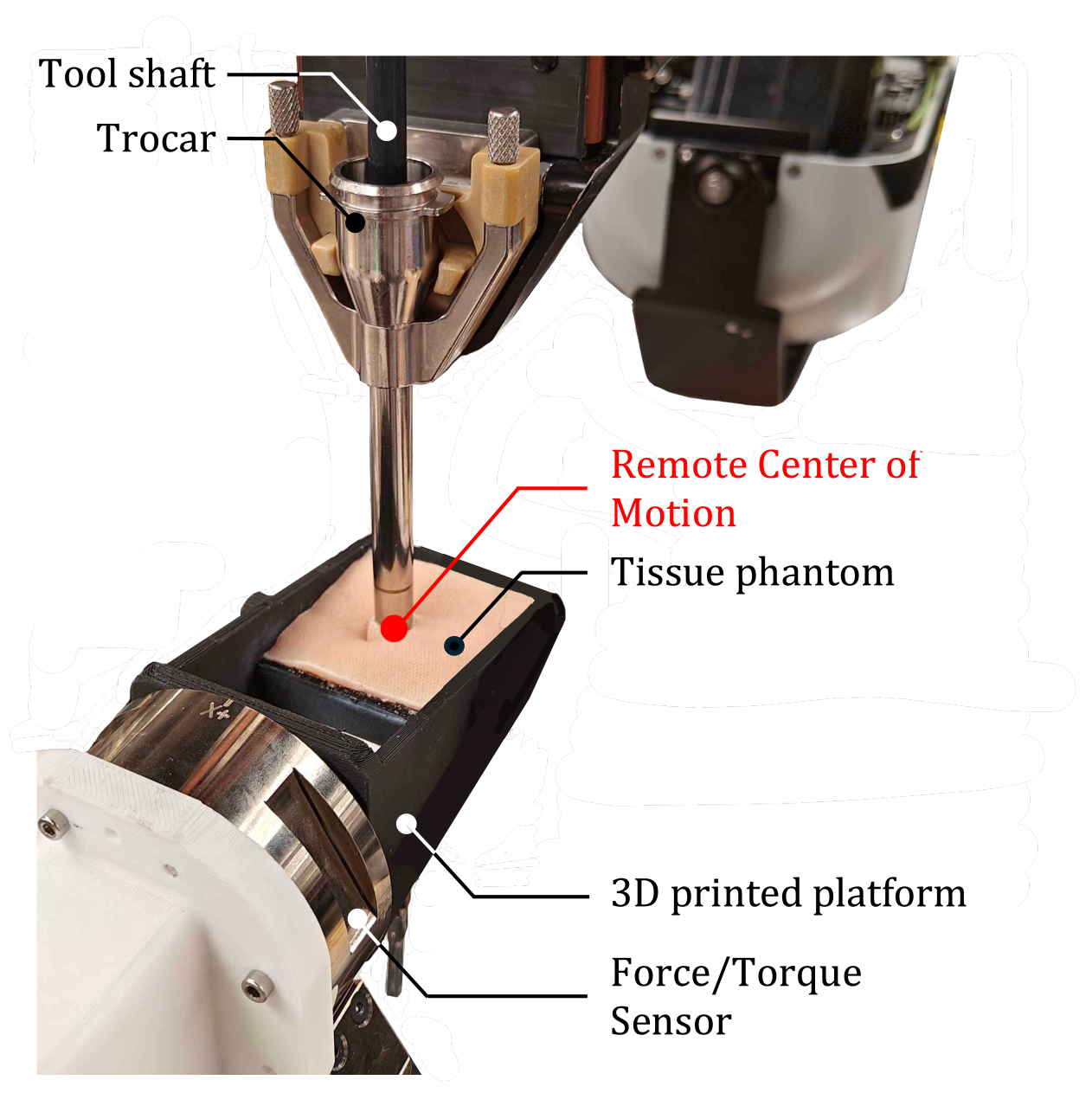
Figure 1: The RCM misalignment estimation setup. A tissue phantom is super-glued to a 3D-printed platform, which, along with the force/torque sensor, is screw-mounted to an adjustable 3-DoF aluminum frame (not shown). The trocar, placed in the phantom, serves as the entry point for the robot tool shaft. A black bar on the trocar marks the robot’s RCM.

This work addresses these gaps in robotic surgical safety by presenting a novel force estimation-based approach to dynamically estimate RCM misalignment during surgical procedures. In particular, our main contributions are: a) experimental quantification of forces exerted on soft tissue due to RCM misalignment, providing reference data for assessing clinical significance of positioning errors in robotic surgical systems; b) development of a deep learning-based framework to accurately estimate forces acting on a surgical tool shaft without need for additional sensors; and c) development of an RCM misalignment estimation approach using predicted tool shaft forces, experimentally validated on the da Vinci Research Kit (dVRK) Classic [10].

II Related Works

II-A RCM Identification Approaches

Various methods have been developed to define RCMs in surgical robotics, broadly categorized as hardware-based (mechanical design) and software-based approaches. Correspondingly, different strategies have been investigated for estimating RCM positioning, including vision-based, sensor-based, and model-based approaches.

Vision-based methods typically employ optical tracking systems to identify the RCM point. Wilson et al. evaluated RCM positioning using computer vision techniques that require dual cameras with direct visual access to the tool shaft - a configuration challenging to implement clinically due to workspace constraints and potential occlusion by surgical instruments [11]. Wang et al. determined the transformation between dual-arm robotic RCMs using only the endoscopic camera without external data sources [12]. While innovative, this approach only establishes relative transformations between dual-arm RCMs rather than maintaining safe RCM positioning relative to patient anatomy. Though theoretically adaptable for RCM repositioning, most vision-based methods function optimally in static environments and face practical limitations from occlusions and dynamic environmental changes.

Sensor-based approaches primarily leverage force/torque sensing to prevent unsafe tissue forces. Fontanelli et al. developed a specialized force sensor for trocar tip attachment, but this does not address RCM repositioning requirements [13]. Nasiri et al. estimated forces at the RCM using force/torque feedback at the robot base to adjust instrument positioning through an admittance controller, minimizing forces at the RCM [8]. However, this approach was validated only on systems with software-based RCMs rather than mechanical implementations.

Model-based approaches incorporate kinematic models and control algorithms to estimate RCM constraints. Dynamic model-based RCM estimation often requires external sensor measurements, as demonstrated in Nasiri et al.’s extended work [14] and Kastrisi et al.’s admittance controller implementations [15]. However, these approaches present integration challenges with mechanically-defined RCM systems due to limited built-in adaptability, complicating model-based correction implementation. Effective solutions will likely require hybrid approaches where software compensation addresses minor misalignments while significant deviations necessitate manual repositioning.

Despite their innovations, existing approaches inadequately address dynamic surgical environment challenges, including sudden force variations and sensor inaccuracies, while requiring complex technical setups that are not practical for clinical implementation. These gaps motivate the development of an advanced force estimation-based RCM identification methodology, capable of real-time adaptation within existing surgical robotic platform constraints.

II-B Force Estimation Techniques

Researchers have developed sensorless force estimation methods, broadly categorized into model-based and learning-based approaches. While model-based methods depend heavily on precise robot modeling, learning-based techniques avoid explicit modeling of complex, nonlinear, and uncertain dynamics by instead identifying patterns from collected data. These sensorless methods primarily estimate free-space joint torque, from which forces can be calculated using the system’s Jacobian matrix. Chua et al. developed a vision and kinematics-based approach to estimate tip forces on the dVRK Classic, though their reliance on external cameras limited clinical applicability [16]. Yilmaz et al. proposed a multi-layer perceptron neural network to estimate free-space joint torque based on kinematics [17]. Wu et al. subsequently extended this approach by implementing a Long Short-Term Memory (LSTM) neural network for improved estimation accuracy and introduced a secondary network to compensate for patient-robot interaction forces [18]. Building on this research trajectory, our team previously developed a hybrid model- and learning-based framework for dVRK Classic force estimation that combines the generalizability of model-based approaches with the adaptability of learning-based methods [19]. To the best of the authors’ knowledge, none of these force estimation techniques have been specifically applied to determine RCM positioning.

III Methods

This section presents the geometric and mathematical formulation of the RCM misalignment problem. We separate the problem into learning-based free-space force estimation, Jacobian derivation at the RCM, and RCM offset optimization.

III-A Problem Formulation

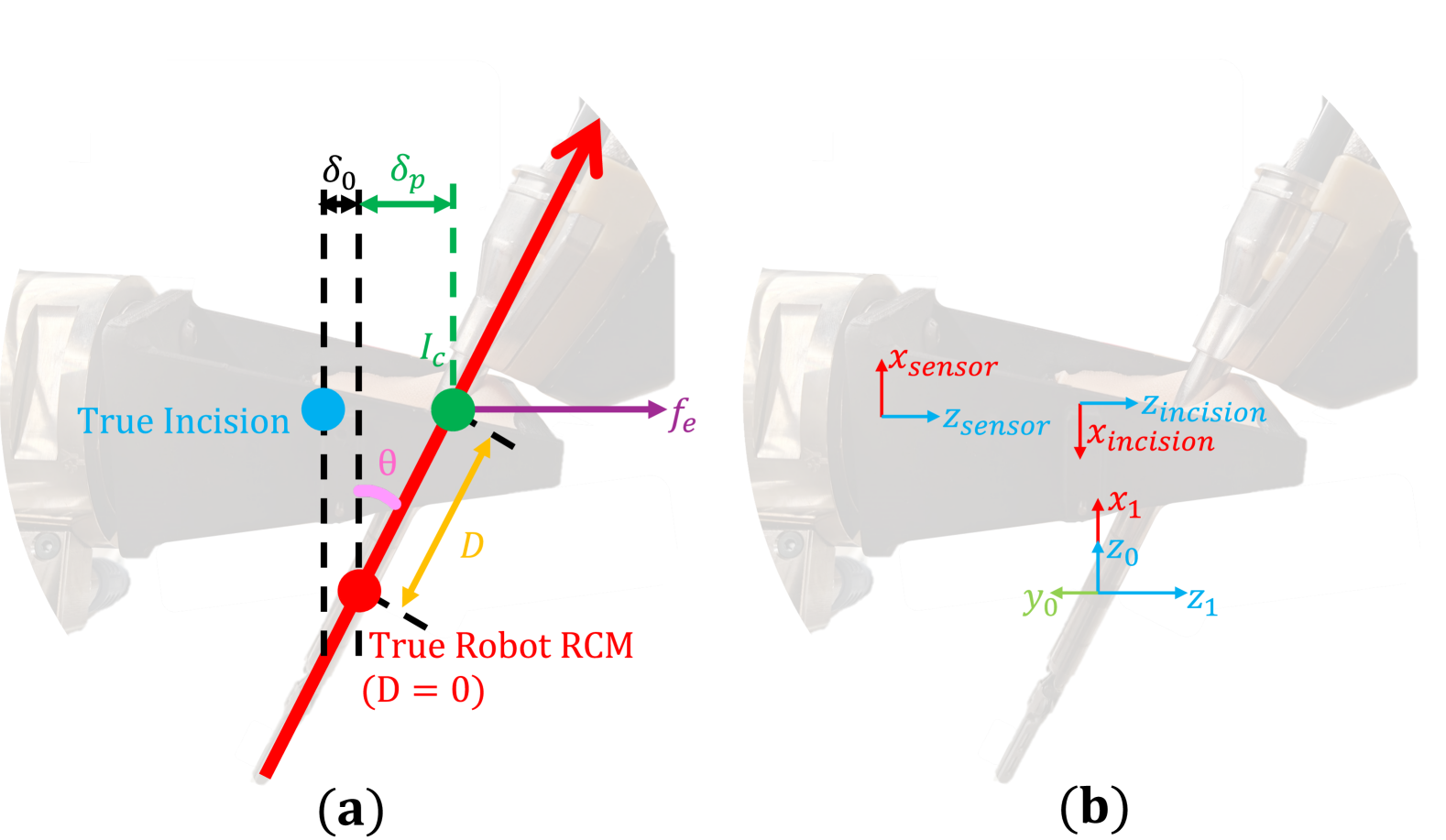
Figure 2: (a) Illustration of the RCM misalignment model, (b) with the corresponding frames assignment.

We propose a model to demonstrate the RCM misalignment problem as shown in Fig. 2. We define the following variables: $f_{e}$ as the interaction force on the environment, $I_{c}$ as the misaligned incision port location, and $D$ as the Euclidean distance from the true RCM to $I_{c}$, with $D$ positive along the robot insertion joint from the RCM to the head of robot instrument. The pivoting angle relative to the true RCM plumb line is $\theta$. Offsets include $\delta$ (true incision to $I_{c}$), $\delta_{p}$ (true RCM plumb line to $I_{c}$, caused by coaxial misalignment), and $\delta_{0}$ (true incision plumb line to the true RCM plumb line, caused by radial misalignment).

The robot joints torques are related to the Cartesian force by the following equation:

$$\mathbf{J}^{\mathrm{T}}{\mathbf{f}_{e}}=\boldsymbol{\tau}-\boldsymbol{\tau}_{0},$$ (1)

where $\mathbf{J}$ is the Jacobian matrix, ${\mathbf{f}_{e}}$ is the external interaction force at the incision, $\boldsymbol{\tau}$ is the sensed joint torque, and $\boldsymbol{\tau}_{0}$ represents the free-space torque caused by gravity, friction, and other intrinsic factors. We obtain $\boldsymbol{\tau}_{0}$ through free-space robot movement, parameterized by either a model-based or learning-based method [18, 20]. Specifically, a neural network is employed to estimate $\boldsymbol{\tau}_{0}$, as detailed in the next subsection.

III-B Learning-based Interaction Force Estimation at Incision

Our learning-based method builds upon the framework of Wu et al. [18], with the only modification of increasing the LSTM hidden dimension from 128 to 512. We train an LSTM network to estimate free-space torques for each joint of the dVRK Classic Patient Side Manipulator (PSM) using joint angles and velocities as inputs. The L2 loss function is used to compare the estimated and measured free-space torques.

We then estimate the external Cartesian force exerted on the robot instrument shaft when in contact with the environment using the following equation:

$$\hat{\mathbf{f}}_{e}=\mathbf{J}^{-\mathrm{T}}(\boldsymbol{\tau}-\boldsymbol{\tau}_{0})=\mathbf{J}^{-\mathrm{T}}(\boldsymbol{\tau}-\hat{\boldsymbol{\tau}}_{\text{LSTM}}).$$ (2)

III-C Jacobian Derivation at Incision

The spatial Jacobian is computed at the incision site, differing from the default Jacobian typically defined at the tool-tip. We begin by adjusting the kinematics and modifying the Denavit-Hartenberg (DH) table. According to the dVRK user manual [21], the robot base frame is defined at the RCM. The analysis is restricted to the DH parameters of the first three joints, as only they are affected by the RCM misalignment. Additionally, in contrast to the dVRK convention, we modify the translation along the local $z$-axis of the third frame to account for the misalignment between the RCM and incision, denoted as $D$. The modified incision port frame is shown in Fig. 2, and the corresponding parameters are shown in Table I. The Jacobian at the incision is given by the following equation:

$$\mathbf{J} ={\small\begin{bmatrix}{{}^{0}\mathbf{R}}_{1}\mathbf{z}_{0}\times(\mathbf{d}_{0}^{3}-\mathbf{d}_{0}^{1})&{{}^{0}\mathbf{R}}_{2}\mathbf{z}_{0}\times(\mathbf{d}_{0}^{3}-\mathbf{d}_{0}^{2})&{{}^{0}\mathbf{R}}_{3}\mathbf{z}_{0}\end{bmatrix}}$$

$$={\footnotesize\begin{bmatrix}-{D}\cos q_{1}\cos q_{2}&{D}\sin q_{1}\sin q_{2}&\cos q_{2}\sin q_{1}\\ 0&{D}\cos q_{2}&-\sin q_{2}\\ -{D}\cos q_{2}\sin q_{1}&-{D}\cos q_{1}\sin q_{2}&-\cos q_{1}\cos q_{2}\end{bmatrix}}$$ (3)

where $\mathbf{z}_{0}=\begin{bmatrix}0,0,1\end{bmatrix}^{T}$, ${{}^{0}\mathbf{R}}_{i}$ is the rotation matrix and $\mathbf{d}_{0}^{i}$ is the position vector of frame $i$ with respect to the robot base frame.

TABLE I: DH table of the PSM modified from [21].

i	Joint type	$a_{i-1}$	$\alpha_{i-1}$	$d_{i}$	$\theta_{i}$
$1$	$revolute$	0	$+\frac{\pi}{2}$	0	$q_{1}+\frac{\pi}{2}$
$2$	$revolute$	0	$-\frac{\pi}{2}$	0	$q_{2}-\frac{\pi}{2}$
$3$	$prismatic$	0	$-\frac{\pi}{2}$	$-D$	0

Note: $a_{i-1}$, $\alpha_{i-1}$, $d_{i}$ and $\theta_{i}$ are the modified DH parameters of link $i$. $q_{i}$ is the joint position of link $i$.

With the modified Jacobian $\mathbf{J}$, the full cost function is formulated and optimized to solve for the unknown variables in the RCM misalignment problem.

III-D RCM Optimization Algorithm

We first use an optimization-based method for force estimation-based RCM estimation, formulated as follows:

$$\begin{split}\operatorname*{argmin}_{k,D}&\quad\frac{1}{2}\hat{\mathbf{{h}}}^{\mathrm{T}}\hat{\mathbf{h}},\\ \operatorname*{subject\,to}&\quad k_{min}\leq k\leq k_{max}\\ &-20\,mm\leq D\leq 50\,mm\end{split}$$ (4)

where $h$ is defined as:

$$\mathbf{h}=\left(\mathbf{f}_{0}+\mathbf{f}_{p}\right)-\mathbf{J}^{-{\mathrm{T}}}\left(\boldsymbol{\tau}-\boldsymbol{\hat{\tau}}_{\text{LSTM}}\right).$$ (5)

The loss function variables are:

• $\mathbf{J}$, the modified Jacobian dependent on $D$, $q_{1}$, and $q_{2}$,

• $\boldsymbol{\tau}$, the measured joints torques,

• $\boldsymbol{\hat{\tau}}_{\text{LSTM}}$, the free-space torques estimated by the LSTM network,

• $\mathbf{f}_{0}=k\delta_{0}\hat{\mathbf{n}}_{0}$, the preloaded radial misalignment force, which is set to 0 under the assumption that radial misalignment is negligible compared to coaxial misalignment,

• $\mathbf{f}_{p}=k\delta_{p}\hat{\mathbf{n}}_{p}$, the RCM-incision coaxial misalignment force with:

  • $\delta_{p}=D\sin\theta$, $\theta=\arccos(\cos q_{1}\cos q_{2})$

  • $\hat{\mathbf{n}}_{p}=\frac{\mathbf{J}^{-{\mathrm{T}}}(\boldsymbol{\tau}-\hat{\boldsymbol{\tau}}_{LSTM})}{||\mathbf{J}^{-{\mathrm{T}}}(\boldsymbol{\tau}-\hat{\boldsymbol{\tau}}_{LSTM})||}$, the unit vector of the estimated overall misalignment force,

• Unknown parameters: $k$, $D$. $D$ represents the Euclidean distance from the true RCM to the misaligned incision port, constrained by the trocar length. The parameter $k$ is somewhat challenging to define. We approximate the misalignment force using a linear spring model, where the force magnitude is $k\delta_{p}$ and its direction is $\hat{\mathbf{n}}_{p}$. Thus, $k$ effectively represents the phantom tissue’s properties, assuming it behaves as an isotropic linear spring. While this assumption may not hold in real scenarios, we adopt it for this feasibility study. We start with an initial guess for $k$’s constraints $[k_{min},k_{max}]$ and discuss how we update them in the following paragraphs.

Thus, Eq. 5 can be rewritten as a function of $k$ and $D$:

$$\mathbf{h}=\left(\frac{kD\sin(\theta)}{||\mathbf{J}^{-{\mathrm{T}}}(\boldsymbol{\tau}-\hat{\boldsymbol{\tau}}_{LSTM})||}-1\right)\mathbf{J}^{-{\mathrm{T}}}(\boldsymbol{\tau}-\hat{\boldsymbol{\tau}}_{LSTM}).$$ (6)

We collect $N$ data points of $\mathbf{q}=[q_{1},q_{2},q_{3}]^{T}$ and $\boldsymbol{\tau}$. Using this data, we compute $\theta(\mathbf{q})$, formulate the expression of $\mathbf{J}(D,\mathbf{q})$, use the LSTM network to estimate the free space torque ${\boldsymbol{\hat{\tau}}}_{\text{LSTM}}$, and optimize the cost function.

With two variables and a single equation, the problem is underconstrained, leading to multiple possible solutions for $k$ and $D$. To address this, we adopt the concept of freeze-unfreeze layers from transfer learning [22, 23]. Specifically, we introduce a two-phase optimization framework that optimizes $k$ and $D$ separately.

For phase 1, we collect dataset with fixed $D^{*},\theta^{*}$. In other words, the input $D^{*}$ is from measurements, and the robot is moved along a pre-defined trajectory:

$$q_{1}=\theta^{*}\cos(\omega t),\quad q_{2}=\theta^{*}\sin(\omega t)$$ (7)

where $\omega$ is the angular velocity and $t$ is the elapsed time. Since force estimation can introduce inaccuracies that would affect the optimization of $k$, in this phase, we use the ground truth force readings $\mathbf{f}_{e}^{*}$ from an ATI force sensor (ATI Industrial Automation, Apex, NC, USA) instead. Therefore, instead of using Eq. 6, we use the following objective function:

$$\mathbf{h}=\left(\frac{kD\sin(\theta^{*})}{||{\mathbf{f}}^{*}_{e}||}-1\right){\mathbf{f}^{*}_{e}}.$$ (8)

In this phase, we use $D^{*}$ as the input to calculate the Jacobian, but we still optimize for both $k$ and $D$. Although the input $D^{*}$ is given and fixed, since $k$ is not fixed, the output $D$ may still vary. We adjust $[k_{min},k_{max}]$ to optimize for a range of $\hat{k}$ such that $D$ remains within $D^{*}\pm e$, where $e$ is the preset acceptable tolerance for $D$.

For phase 2, we collect datasets with teleoperation and the estimated $\hat{k}$ from phase 1. Since $\theta$ is no longer fixed, we compute it for each configuration. We then estimate the external force using the learning-based method and optimize for $D$ using Eq. 6. The entire optimization algorithm is shown in Algorithm 1.

Algorithm 1 Force Estimation-Based Two-Phase Alternating Optimization of $k$ and $D$

1:Input: ${q}_{j,i}$, $\boldsymbol{\tau}_{i}$, for $i=1,\dots,N$ and $j=1,2,3$, bounds $k_{\min},k_{\max},D_{\min},D_{\max}$, error $e$ for acceptable $D$.

2:Output: Optimized parameters $\hat{k}$, $\hat{D}$.

3:Initialize $k$, $D$ with random values or prior estimates.

4:// Phase 1: Optimize $k$ with $D^{*},\theta^{*}$ fixed

5:for each set of $[D^{*},\theta^{*}]$ do

6:  for $i=1$ to $N_{1}$ do

7:   Compute $\mathbf{J}_{i}(D^{*},q_{j})$.

8:   Estimate $\boldsymbol{\tau}_{0,i}=\hat{\boldsymbol{\tau}}_{LSTM,i}$.

9:   Compute $\mathbf{h}_{i}=\left(\frac{kD\sin(\theta^{*})}{|\mathbf{f}^{*}_{e}|}-1\right)\mathbf{f}^{*}_{e}$.

10:   Compute the cost function: $C_{i}=\frac{1}{2}\mathbf{h}_{i}^{\mathrm{T}}\mathbf{h}_{i}$.

11:  end for

12:  Compute the total cost: $C=\sum_{i=1}^{N_{1}}C_{i}$.

13:  Use a gradient-based optimization method (e.g., Levenberg-Marquardt [24] or fmincon [25]) to minimize $C$ with respect to $k$ and $D$.

14:  while not converged OR $|D^{*}-D|>e$ do

15:   Update $k_{\min},k_{\max}$.

16:   Recompute $C$ using the updated parameters.

17:  end while

18:  Find range $\hat{k}=[L,R]$ for $D^{*}\pm e$.

19:end for

20:Compute the smallest common range of $\hat{k}$. Fix $\hat{k}$ using the midpoint of this common range.

21:// Phase 2: Optimize $D$ with $\hat{k}$ fixed

22:for $m=1$ to $N_{2}$ do

23:  Compute $\theta_{m}=\arccos(\cos(q_{1,m})\cos(q_{2,m}))$.

24:  Compute $\mathbf{J}_{m}(D,q_{j})$.

25:  Estimate $\boldsymbol{\tau}_{0,m}=\hat{\boldsymbol{\tau}}_{LSTM,m}$.

26:  Compute $\mathbf{h}_{m}=\left(\frac{kD\sin(\theta_{m})}{|\mathbf{J}_{m}^{-\mathrm{T}}(\boldsymbol{\tau}_{m}-\hat{\boldsymbol{\tau}}_{LSTM,m})|}-1\right)\mathbf{J}_{m}^{-\mathrm{T}}(\boldsymbol{\tau}_{m}-\hat{\boldsymbol{\tau}}_{LSTM,m})$.

27:  Compute the cost function: $C_{m}=\frac{1}{2}\mathbf{h}_{m}^{\mathrm{T}}\mathbf{h}_{m}$.

28:end for

29:Compute the total cost: $C=\sum_{m=1}^{N_{2}}C_{m}$.

30:Use a gradient-based optimization method to minimize $C$ with respect to $D$. Find the optimal $\hat{D}$.

31:Return Optimized parameters $\hat{k},\hat{D}$.

IV Experimental Setup

IV-A Hardware Setup

We build a 3-DoF aluminum frame with an adjustable moving platform, as shown in Fig. 1. The platform includes an ATI force sensor for ground truth force readings, and a 3D-printed tissue holder with a 3-layer silicone tissue sample. In this setup, we can directly measure the ground truth incision misalignment, $D^{*}$, and the ground truth interaction force at the incision, $f^{*}_{e}$, to validate our optimization results.

IV-B Demonstration of Necessity Experimental Setup

Before validating our algorithm, we first assess whether extreme RCM misalignment induces significant forces. Using the hardware setup in Section IV-A, we insert the trocar through phantom tissue affixed to a 3D-printed platform, measuring the ground-truth interaction force. To achieve different misalignment distances, we move the robot to various positions such that $\theta$ changes. We then record the static force for each combination of $D$ and $\theta$ and plot the force-angle relationship.

IV-C RCM Misalignment Force Estimation Experimental Setup

IV-C1 Free Space Joint Torque Data Collection and Training

The free-space training dataset for the dVRK PSM is collected through teleoperation for approximately 15 minutes, with the robots moving without contacting the environment. We split the datasets into 70% for training, 20% for validation, and 10% for testing. The hyperparameter settings, the structure of the neural network and the devices used are consistent with those in our previous work [26, 19].

IV-C2 RCM Misaligned Force Estimation

We intend to verify Eq. 2 and Eq. III-C in this experiment. In our previous works [18, 17, 19], we demonstrated the effectiveness of Eq.2 for external tip contact. In[19], we used a secondary network to compensate for incision interaction force, but did not analyze its magnitude. In this work, we exclude tip contact, so the external force results solely from trocar-phantom interaction. We place the moving platform at a randomly chosen misalignment, $D=30\,mm$, and collect a 1-minute test dataset while tele-operating the robot. We then compute the estimated force using Eq.2 with the Jacobian from Eq.III-C, comparing the result with ground truth data from the ATI force sensor to assess estimation accuracy.

IV-D RCM Optimization Experimental setup

IV-D1 Fixing $D,\theta$, Optimizing for $k$: Pivoting Motion

As described in Section 1, we first use a well-structured experimental setup to optimize the range of $k$. We conduct multiple trials, each with a fixed $\theta^{*}$ and measured $D^{*}$ to optimize $k$. We use a Python script to have the robot following a pre-defined pivoting motion (Eq.7), with RCM misalignment $D^{*}$. We collect joint position and torque data, for six sets of $[D^{*},\theta^{*}]$: [15, 15], [15, 30], [15, 45], [30, 15], [30, 30], and [45, 15]. We implement phase 1 of Algorithm1 in Matlab using lsqnonlin[27] as the solver and Trust-Region-Reflective[28, 25] as the optimization algorithm. We set the tolerance error $e=$ 2 mm.

IV-D2 Fixing $k$, Optimizing for $D$: Tele-operation

After we find the optimized $\hat{k}$ to use, we fix $\hat{k}$ and optimize for $D$. We collect several new test dataset with $D^{*}$ uniformly chosen from $[D_{min},D_{max}]$ = [-20 mm, 50 mm]. We teleoperate the robot and collect data under these misalignments. Phase 2 of Algorithm 1 is implemented in Matlab using the same solver and algorithm as in phase 1. We then compare the optimized $\hat{D}$ with the ground truth $D^{*}$ to validate the algorithm.

V Results and Discussion

V-A Demonstration of the Necessity for RCM Estimation

We follow the experimental setup in Section IV-B. At the RCM, the interaction force should be zero or near zero due to its mechanical properties. At the misaligned incision port, a larger interaction force is expected. Additionally, as $\theta$ increases, the interaction force should also increase. The results are shown in Fig. 3.

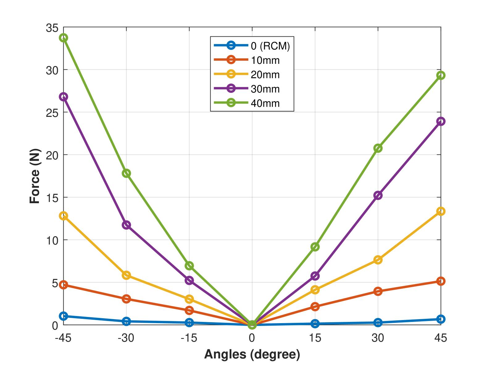
Figure 3: Static force-angle plot in different misalignment distances. Maximum force is about 40 N, which is a large force that could potentially cause damage on the incision tissue.

Our experiment shows that when the incision port is over 20 mm from the RCM, an interaction force exceeding 12 N is exerted on the patient. For $[D,\theta]$=[40 mm, 45^∘], the force reaches 35 N, which could potentially damage abdominal tissue. This highlights the need to detect and correct RCM misalignment during da Vinci robot surgery.

V-B Interaction Force Estimation at Misaligned RCM

Following the setup in Section IV-C, results in Fig. 4 and Table II show root mean squared errors (RMSE) of 1-2 N in each direction, comparable to prior studies [18, 26, 19]. This demonstrates the generalizability of our force estimation method from tool tip to misaligned RCM (incision port).

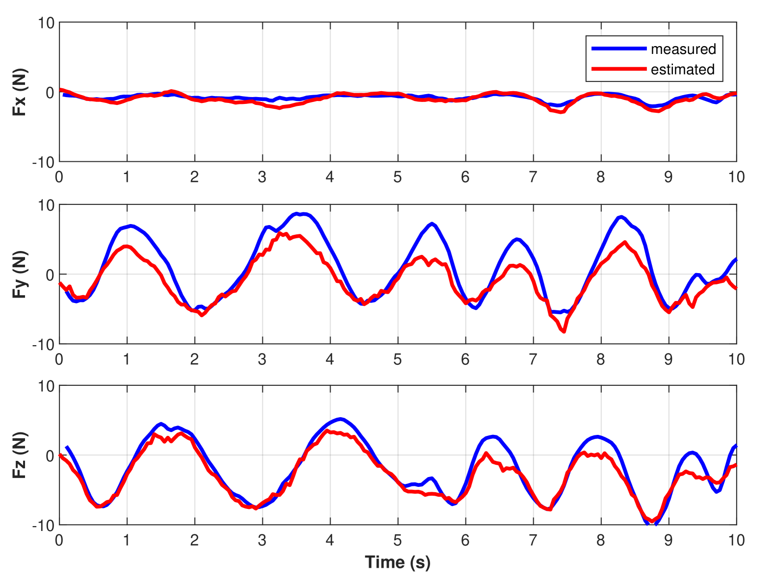
Figure 4: Cartesian force estimation at the incision port, where it is misaligned with respect to the RCM for 30 mm. Our learning-based force estimation tracks ground truth force measurements well.

TABLE II: RMSE of Incision Interaction Cartesian Force Estimation

Method	$Fx(N)$	$Fy(N)$	$Fz(N)$
Proposed	1.29	2.24	1.81
[18]*	2.3	1.5	3.3
[26]*	1.08	0.9	0.89

V-C Optimization for RCM Misalignment

As mentioned in Section III-D, we first do phase 1 to optimize for $k$ with fixed $D^{*},\theta^{*}$ and expect a range of $k$. The $k$ ranges associated with different configurations are shown in Table III. We find that $k=900$ is the midpoint of the smallest common of these ranges.

TABLE III: Ranges of $k$ with Fixed $D$ under Different Configurations

$D^{*}$ (mm)	$\theta^{*}$ (∘)	$\hat{k}$
$15\pm 2$	15	750 ~ 850
	30	700 ~ 800
	45	950 ~ 1110
$30\pm 2$	15	850 ~ 950
	30	1050 ~ 1150
$45\pm 2$	15	860 ~ 910

In phase 2, we fix $\hat{k}=900$ and optimize for $D$ using the teleoperating test datasets. We intentionally select $D^{*}$s values different from phase 1 to assess generalizability to out-of-distribution inputs. The results are shown in Table IV.

TABLE IV: Optimized $D$ with Fixed $k$ under Different Misalignment

$k$	$D^{*}$ (mm)	$\hat{D}$ (mm)	$e_{abs}$ (mm)
900	-20.0	24.8	4.8
	-10.0	18.0	8
	0.0 (RCM)	17.7	17.7
	10.0	18.3	8.3
	20.0	21.5	1.5
	30.0	32.0	2,0
	40.0	36.9	3.1

We observe that with our optimization scheme and the selected fixed $\hat{k}$, the absolute error $e_{abs}=|D^{*}|-|\hat{D}|$ is within 5 mm for any $D^{*}\geq 20$ mm. Therefore, when the RCM is misaligned further than 20 mm, our optimization scheme works well.

V-D Discussion

Through our results, we show that when the RCM is misaligned far enough (further than 20 mm), our framework is effective. We also show that this method generalizes, as we do not train with negative $D$, but our algorithm still achieves acceptable error for negative values.

TABLE V: Optimized $D$ with Fixed $k$ within Misalignment $\pm 10$ mm

$k$	$D^{*}$ (mm)	$\hat{D}$ (mm)	$e_{abs}$ (mm)
900	-10.0	9.0	1.0
	0.0 (RCM)	2.1	2.1
	10.0	7.3	2.7

While optimization within $\pm 10$ mm misalignment achieved higher error, this may be ameliorated with better force estimation algorithm. From our experience, any sensorless force estimation scheme (either model-based or learning-based) generates poor RCM estimates with a small external force (e.g. $\leq 5\,N$). To justify this, we repeat the optimization for $D^{*}$=[-10, 0, 10] with the ground truth force measurements using Eq.8 and the teleoperation test datasets. The results are shown in Table V. The absolute errors in this case are small. While the dependence on accurate force estimation is a limitation of our work, we argue that the optimization scheme itself is globally effective for such well-structured experimental setups.

Another limitation is that the current optimization formulation cannot account for signed offset in the RCM due to the squared term in the optimization function. Lastly, we only validated that our framework works under a well-structured experimental setup. We acknowledge that we have a strong and likely unrealistic assumption that $k$ remains nearly constant for our tissue phantom, oversimplifying the tissue as an isotropic linear spring. Moreover, in our setup, we must actively interact with the environment to determine the RCM offsets, which does not directly align with real scenarios. Again, we emphasize that this work is a feasibility study. In the future, we aim to estimate $k$ without direct patient interaction, such as through animal or cadaver studies, followed by transfer learning to develop a more accurate tissue model for RCM misalignment estimation. Ultimately, further work is needed to validate our method in thicker, more heterogeneous, and more realistic tissues.

VI Conclusion and Future work

We propose a sensorless framework to optimize for the RCM misalignment. Through our experiments, we show that misalignment can potentially generate enough force to damage tissue . For misalignments larger than 20 mm, our proposed algorithm is effective at estimating the misalignment. As future work, we plan to add a term in the cost function to penalize signs or determine the sign based on estimated force, investigate methods for improving small force estimation such as filtering or faster data collection, and extend our algorithm to more clinical applicable setups. Accurately estimating the RCM misalignment is a step toward automation compensation and thus, reducing damage to tissue at incision point.

References

- [1] V. Velanovich, “Laparoscopic vs open surgery: a preliminary comparison of quality-of-life outcomes,” Surgical endoscopy, vol. 14, pp. 16–21, 2000.
- [2] J. E. Varela, S. E. Wilson, and N. T. Nguyen, “Laparoscopic surgery significantly reduces surgical-site infections compared with open surgery,” Surgical endoscopy, vol. 24, pp. 270–276, 2010.
- [3] R. H. Taylor, P. Kazanzides, G. S. Fischer, N. Simaan, and D. D. Feng, “Chapter nineteen—medical robotics and computer-integrated interventional medicine,” Biomedical Information Technology, 2nd ed.; Feng, DD, Ed.; Biomedical Engineering, Academic Press: Cambridge, MA, USA, pp. 617–672, 2020.
- [4] C.-H. Kuo and J. S. Dai, “Robotics for minimally invasive surgery: a historical review from the perspective of kinematics,” in International Symposium on History of Machines and Mechanisms: Proceedings of HMM 2008. Springer, 2009, pp. 337–354.
- [5] S. K. Pandey and V. Sharma, “Robotics and ophthalmology: Are we there yet?” Indian Journal of Ophthalmology, vol. 67, no. 7, pp. 988–994, 2019.
- [6] C. N. Riviere, J. Gangloff, and M. De Mathelin, “Robotic compensation of biological motion to enhance surgical accuracy,” Proceedings of the IEEE, vol. 94, no. 9, pp. 1705–1716, 2006.
- [7] B. Rosa, C. Gruijthuijsen, B. Van Cleynenbreugel, J. V. Sloten, D. Reynaerts, and E. V. Poorten, “Estimation of optimal pivot point for remote center of motion alignment in surgery,” International journal of computer assisted radiology and surgery, vol. 10, pp. 205–215, 2015.
- [8] E. Nasiri and L. Wang, “Admittance control for adaptive remote center of motion in robotic laparoscopic surgery,” in 2024 21st International Conference on Ubiquitous Robots (UR). IEEE, 2024, pp. 51–57.
- [9] M. Nathan, “The senhance® surgical system,” Robotic Surgery, pp. 159–163, 2021.
- [10] P. Kazanzides, Z. Chen, A. Deguet, G. S. Fischer, R. H. Taylor, and S. P. DiMaio, “An open-source research kit for the da vinci surgical system,” in IEEE Intl. Conf. on Robotics and Auto. (ICRA), Hong Kong, China, 2014, pp. 6434–6439.
- [11] J. T. Wilson, T.-C. Tsao, J.-P. Hubschman, and S. Schwartz, “Evaluating remote centers of motion for minimally invasive surgical robots by computer vision,” in 2010 IEEE/ASME International Conference on Advanced Intelligent Mechatronics. IEEE, 2010, pp. 1413–1418.
- [12] Z. Wang, Z. Liu, Q. Ma, A. Cheng, Y.-h. Liu, S. Kim, A. Deguet, A. Reiter, P. Kazanzides, and R. H. Taylor, “Vision-based calibration of dual rcm-based robot arms in human-robot collaborative minimally invasive surgery,” IEEE Robotics and Automation Letters, vol. 3, no. 2, pp. 672–679, 2017.
- [13] G. A. Fontanelli, L. R. Buonocore, F. Ficuciello, L. Villani, and B. Siciliano, “A novel force sensing integrated into the trocar for minimally invasive robotic surgery,” in 2017 IEEE/RSJ International Conference on Intelligent Robots and Systems (IROS). IEEE, 2017, pp. 131–136.
- [14] E. Nasiri, S. Sowrirajan, and L. Wang, “Teleoperation in robot-assisted mis with adaptive rcm via admittance control,” International Journal of Intelligent Robotics and Applications, pp. 1–13, 2024.
- [15] T. Kastritsi and Z. Doulgeri, “A controller to impose a rcm for hands-on robotic-assisted minimally invasive surgery,” IEEE Transactions on Medical Robotics and Bionics, vol. 3, no. 2, pp. 392–401, 2021.
- [16] Z. Chua and A. M. Okamura, “Characterization of real-time haptic feedback from multimodal neural network-based force estimates during teleoperation,” 2022 IEEE/RSJ International Conference on Intelligent Robots and Systems (IROS), pp. 1471–1478, 2021.
- [17] N. Yilmaz, J. Y. Wu, P. Kazanzides, and U. Tumerdem, “Neural network based inverse dynamics identification and external force estimation on the da vinci research kit,” 2020 IEEE International Conference on Robotics and Automation (ICRA), pp. 1387–1393, 2020.
- [18] J. Y. Wu, N. Yilmaz, U. Tumerdem, and P. Kazanzides, “Robot force estimation with learned intraoperative correction,” 2021 International Symposium on Medical Robotics (ISMR), pp. 1–7, 2021.
- [19] H. Yang, H. Zhou, G. S. Fischer, and J. Y. Wu, “A hybrid model and learning-based force estimation framework for surgical robots,” in 2024 IEEE/RSJ International Conference on Intelligent Robots and Systems (IROS). IEEE, 2024, pp. 906–912.
- [20] Y. Wang, R. Gondokaryono, A. Munawar, and G. S. Fischer, “A convex optimization-based dynamic model identification package for the da vinci research kit,” IEEE Robotics and Automation Letters, vol. 4, pp. 3657–3664, 2019.
- [21] “da vinci research kit user guide,” 2019. [Online]. Available: https://research.intusurg.com/images/2/26/User_Guide_DVRK_Jan_2019.pdf
- [22] J. Yosinski, J. Clune, Y. Bengio, and H. Lipson, “How transferable are features in deep neural networks?” ArXiv, vol. abs/1411.1792, 2014.
- [23] P. Team, “Transfer learning tutorial,” 2024, accessed: 2025-02-28. [Online]. Available: https://pytorch.org/tutorials/beginner/transfer_learning_tutorial.html
- [24] C. T. Kelley, Iterative Methods for Optimization, ser. Frontiers in Applied Mathematics. Philadelphia, PA: SIAM, 1999, vol. 18.
- [25] T. F. Coleman and Y. Li, “An interior trust region approach for nonlinear minimization subject to bounds,” SIAM J. Optim., vol. 6, pp. 418–445, 1993.
- [26] H. Yang, A. Acar, K. Xu, A. Deguet, P. Kazanzides, and J. Y. Wu, “An effectiveness study across baseline and neural network-based force estimation methods on the da vinci research kit si system,” arXiv preprint arXiv:2405.07453, 2024.
- [27] J. DENNIS, “Nonlinear least squares,” State of the Art in Numerical Analysis, pp. 269–312, 1977.
- [28] T. Coleman and Y. li, “On the convergence of reflective newton methods for large-scale nonlinear minimization subject to bounds,” Math. Program., vol. 67, pp. 189–224, 10 1994.