Practical Abstractions for Model Checking
Continuous-Time Multi-Agent Systems

Abstract.

Model checking of temporal logics in a well established technique to verify and validate properties of multi-agent systems (MAS). However, practical model checking requires input models of manageable size. In this paper, we extend the model reduction method by variable-based abstraction, proposed recently by Jamroga and Kim, to the verification of real-time systems and properties. To this end, we define a real-time extension of MAS graphs, extend the abstraction procedure, and prove its correctness for the universal fragment of Timed Computation Tree Logic (TCTL). Besides estimating the theoretical complexity gains, we present an experimental evaluation for a simplified model of the Estonian voting system and verification using the Uppaal model checker.

1. Introduction

Temporal logics have been extensively used to formalize properties of agent systems, including reachability, liveness, safety, and fairness Emerson (1990). Moreover, temporal model checking is a popular approach to formal verification of MAS Baier and Katoen (2008); Clarke et al. (2018). However, the verification is known to be hard, both theoretically and in practice. State-space explosion is a major obstacle here, as models of real-world systems are huge and infeasible even to generate, let alone verify. In consequence, model checking of MAS w.r.t. their modular representations ranges from $\mathbf{{PSPACE}}$-complete to undecidable Schnoebelen (2003); Bulling et al. (2010).

Much work has been done to contain the state-space explosion by smart representation and/or reduction of input models. Symbolic model checking based on SAT- or BDD-based representations of the state/transition space McMillan (1993, 2002); Penczek and Lomuscio (2003); Kacprzak et al. (2004); Lomuscio and Penczek (2007); Huang and Van Der Meyden (2014); Lomuscio et al. (2017) fall into the former group. Model reduction methods include partial-order reduction Peled (1993); Gerth et al. (1999); Jamroga et al. (2020), equivalence-based reductions De Bakker et al. (1984); Alur et al. (1998); Belardinelli et al. (2021), and state abstraction Cousot and Cousot (1977), see below for a detailed discussion.

In this paper, we extend the idea of variable-based abstraction Jamroga and Kim (2023a, b) to the verification of real-time multi-agent systems Alur et al. (1993); Brihaye et al. (2007); Arias et al. (2023); Penczek and Pólrola (2006). Similarly to Jamroga and Kim (2023a, b), our abstraction operates entirely on the high-level, modular representation of an asynchronous MAS. That is, it takes a concrete modular representation of a MAS as input, and generates an abstract modular representation as output. Moreover, it produces the abstract representation without generation of the explicit state model, thus avoiding the usual computational bottleneck.

Related Work. State abstraction was introduced in Cousot and Cousot (1977), and studied intensively in the context of temporal verification Clarke et al. (1994); Godefroid and Jagadeesan (2002); Dams and Grumberg (2018); Clarke et al. (2000); Shoham and Grumberg (2004); Clarke et al. (2000, 2003); Cimatti et al. (2002). However, those works propose lossless abstraction that typically obtain up to an order of magnitude reduction of the state space and output models that are still too large for practical verification. Here, we focus on lossy may abstractions, based on user-defined equivalence relations Dams et al. (1997); Godefroid et al. (2001); Godefroid and Jagadeesan (2002); Godefroid (2014); Gurfinkel et al. (2006); Godefroid et al. (2010); Enea and Dima (2008); Cohen et al. (2009); Lomuscio et al. (2010).

May/must abstractions for strategic properties have been investigated in de Alfaro et al. (2004); Ball and Kupferman (2006); Kouvaros and Lomuscio (2017); Belardinelli and Lomuscio (2017); Belardinelli et al. (2019). In all those cases, the abstraction method is defined directly on the concrete model, i.e., it requires to first generate the concrete global states and transitions, which is exactly the bottleneck that we want to avoid. In contrast, our method operates on modular (and compact) model specifications, both for the concrete and the abstract model. Data abstraction methods for infinite-state MAS Belardinelli et al. (2011, 2017) come close in that respect, but they still generate explicit state models. Even closer, Jamroga and Kim (2023a, b) proposed recently a user-friendly abstraction scheme via removal of variables in the modular agent templates. However, all the above approaches deal only with the verification of untimed models and properties.

Timed models of MAS and their verification have been studied for over 30 years now, see e.g. Alur et al. (1993); Brihaye et al. (2007); Arias et al. (2023) and especially Penczek and Pólrola (2006) for an overview. Time-abstracting bisimulation for timed automata was studied in Tripakis and Yovine (2001). In this paper, we extend the ideas and results from Jamroga and Kim (2023a) to models of real-time asynchronous MAS of Arias et al. (2023).

The study of MAS using Uppaal was conducted in Gu et al. (2022a) and Gu et al. (2022b). However, its authors tackled a different problem — strategy synthesis, in a different setting — stochastic timed games. In some ways, their methods can be seen as complementary to ours, as they first synthesize the (witness) strategy and then check its validity; whereas we mainly focus on the verification of safety properties.

2. Reasoning about Real-Time MAS

We start with extending the (untimed) representations of asynchronous MAS in Jamroga and Kim (2023a) to their timed counterparts.

We first adopt the usual definitions of clocks in timed systems, e.g. Alur et al. (1993). Let $\mathcal{X}=\{{x_{1},\ldots,x_{n_{\mathcal{X}}}}\}$ be a finite set of clock variables. A clock valuation is a mapping $\upsilon:\mathcal{X}\mapsto\mathbb{R}_{+}$. Given a valuation $\upsilon$, a delay $\delta\in\mathbb{R}_{+}$ and $X\subseteq\mathcal{X}$, $\upsilon+\delta$ denotes the valuation $\upsilon^{\prime}$, such that $\upsilon^{\prime}(x)=\upsilon(x)+\delta$ for all $x\in\mathcal{X}$, and $\upsilon[X=0]$ denotes the valuation $\upsilon^{\prime\prime}$, such that $\upsilon^{\prime\prime}(x)=0$ for all $x\in X$ and $\upsilon^{\prime\prime}(x)=\upsilon(x)$ for all $x\in\mathcal{X}\setminus X$.

The set $\mathcal{C}_{\mathcal{X}}$ of clock constraints over $\mathcal{X}$ is inductively defined by the following grammar:

$$\mathfrak{cc}::=\top\ \mid\ x_{i}\sim c\ \mid\ x_{i}-x_{j}\sim c\ \mid\ \mathfrak{cc}\wedge\mathfrak{cc},$$

where $\top$ denotes the truth value, $\forall_{i,j\in\{{1,\ldots,n_{\mathcal{X}}}\}}x_{i},x_{j}\in\mathcal{X}$, $c\in\mathbb{N}$, and ${\sim}\in\{{<,\leq,=,\geq,>}\}$.

Let $\mathcal{V}=\{{v_{1},\ldots,v_{n_{\mathcal{V}}}}\}$ be a finite set of discrete (typed) numeric variables over finite domains. By $\mathit{Eval}_{\mathcal{V}}$ we denote the set of evaluations over the set of (discrete) variables $\mathcal{V}$; an evaluation $\eta\in\mathit{Eval}_{\mathcal{V}}$ maps every variable $v\in\mathcal{V}$ to a literal from their domain $\eta(v)\in domain(v)$. Expressions are constructed from variables $\mathcal{V}$ and literals $\bigcup_{i=1}^{n_{\mathcal{V}}}domain(v_{i})$ using the arithmetic operators. Atomic formulas/conditions are built from expressions and relation symbols. They can be further combined with logical connectives to form predicates. The set of all possible predicates over the variables $\mathcal{V}$ is denoted by $\mathit{Cond}_{\mathcal{V}}$.

The sets of all valuations satisfying $\mathfrak{cc}\in\mathcal{C}_{\mathcal{X}}$ and all evaluations satisfying $g\in\mathit{Cond}_{\mathcal{V}}$ shall be denoted by $\llbracket{\mathfrak{cc}}\rrbracket$ and $\llbracket{g}\rrbracket$ respectively. For $v\in\mathcal{V}$, $k\in domain(v)$, by $g[v=k]$ we denote the substitution of all occurrences of the variable $v$ in $g$ with the literal $k$; analogously, for $V\subseteq\mathcal{V}$, $K=\{{k_{v}\in domain(v)\mid v\in V}\}$, by $g[V=K]$ we denote $g[v=k_{v}\mid v\in\mathcal{V}]$.

For simplicity, we assume that both $\mathcal{X}$ and $\mathcal{V}$ have (some) ordering fixed. In the sequel, the terms variables and clocks will mean discrete variables and continuous variables respectively.

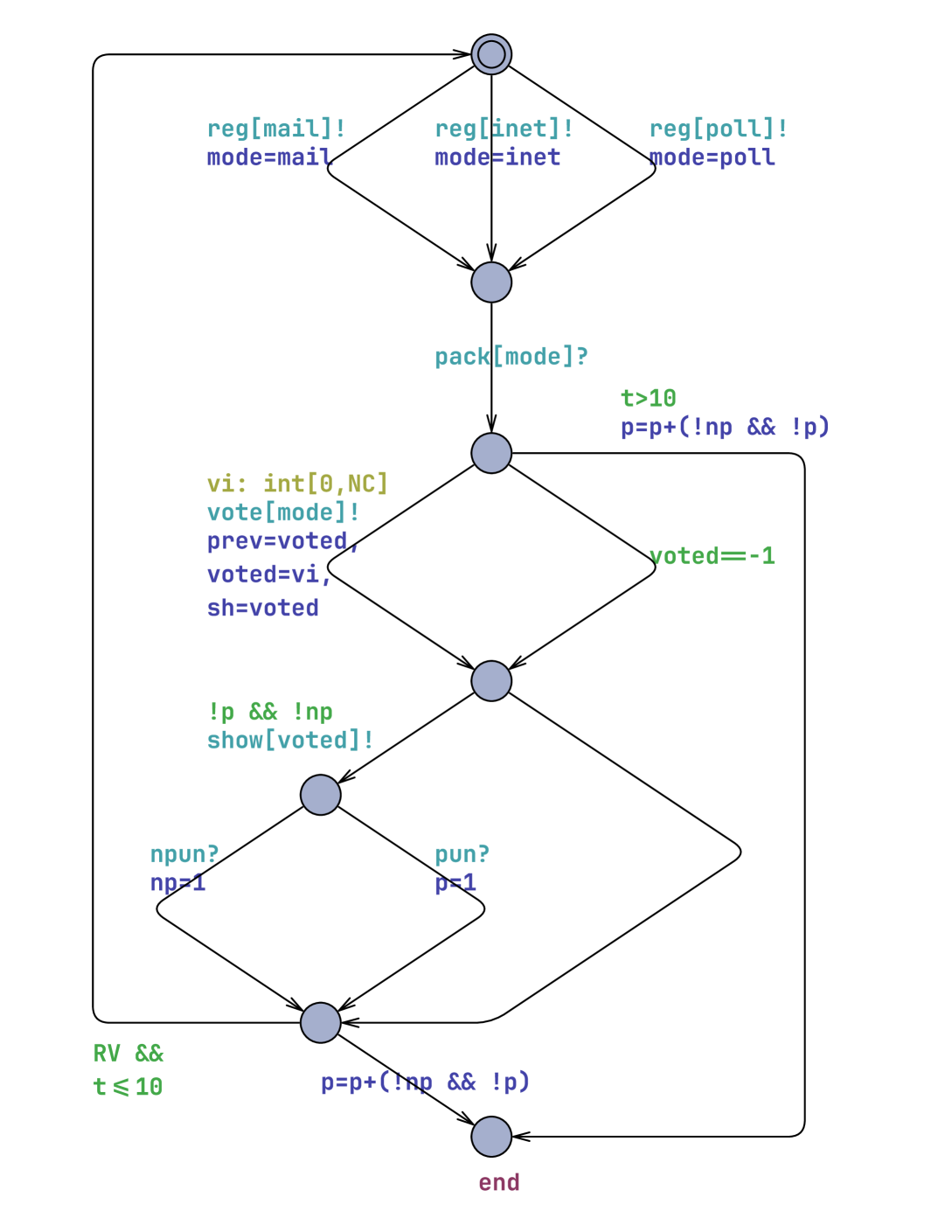
Figure 1. Timed agent graph for the Voter

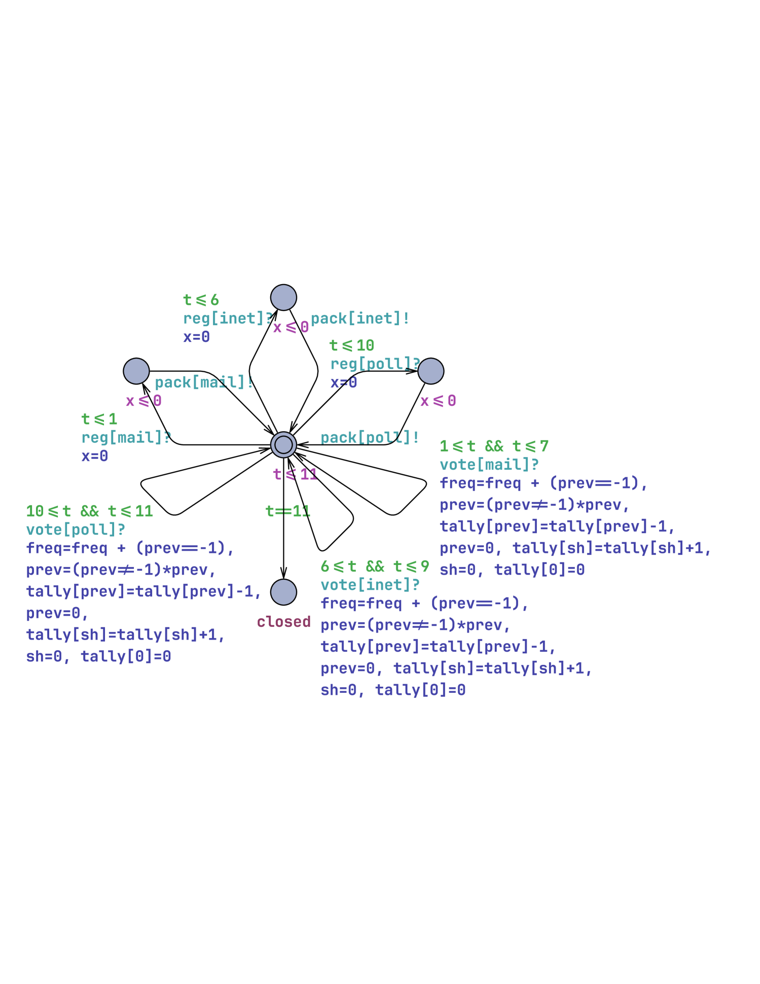
Figure 2. Timed agent graph for the Authority

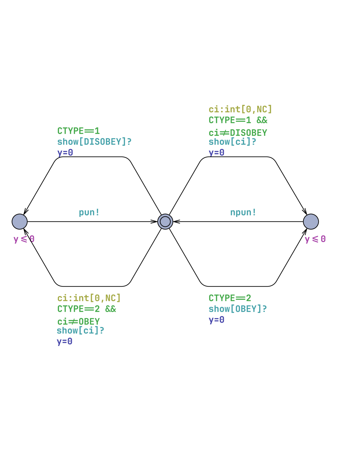
Figure 3. Timed agent graph for the Coercer

2.1. Multi-Agent Graphs with Clocks

In this section, we first introduce the specification of an individual agent, and a set of agents. The associated model is then defined, as well as its behaviour.

Definition (TAG).

A timed agent graph (TAG) is a 10-tuple $G=(\mathcal{V},\mathit{Loc},l_{0},g_{0},\mathit{Act},\mathit{Effect},\mathit{Chan},\mathcal{X},\mathcal{I},E)$, where:

• $\mathcal{V}$ is a finite set of variables,

• $\mathit{Loc}$ is a finite set of locations, $l_{0}\in\mathit{Loc}$ is the initial location,

• $g_{0}\in\mathit{Cond}_{\mathcal{V}}$ is the initial condition, s.t. ${\left.\kern-1.2pt\llbracket{g_{0}}\rrbracket\right|_{\mathcal{V}}}$ is a singleton,

• $\mathit{Act}$ is a set of actions, where $\tau\in\mathit{Act}$ stands for “do nothing”,

• $\mathit{Effect}:\mathit{Act}\times\mathit{Eval}_{\mathcal{V}}\mapsto\mathit{Eval}_{\mathcal{V}}$ is the effect function, such that $\mathit{Effect}(\tau,\eta)=\eta$ for any $\eta\in\mathit{Eval}_{\mathcal{V}}$,

• $\mathit{Chan}$ is a finite set of asymmetric one-to-one synchronisation channels; by $\mathit{Sync}$ we denote the set of synchronisation labels of the form “$ch!$” and “$ch?$” for emitting and receiving on a channel $ch\in\mathit{Chan}$ respectively, and “$-$” for no synchronisation,

• $\mathcal{X}$ is a finite set of clocks,

• $\mathcal{I}:\mathit{Loc}\mapsto\mathcal{C}_{\mathcal{X}}$ is a location invariant,

• $E\subseteq\mathit{Loc}\times\mathit{Cond}_{\mathcal{V}}\times\mathcal{C}_{\mathcal{X}}\times\mathit{Sync}\times\mathit{Act}\times\mathcal{P}({\mathcal{X}})\times\mathit{Loc}$ is a finite set of labelled edges, which define the local transition relation.

Following the common practice, the notation $l\xhookrightarrow{g,\mathfrak{cc},\varsigma,\alpha,X}l^{\prime}$ shall be used as a shorthand for $(l,g,\mathfrak{cc},\varsigma,\alpha,X,l^{\prime})\in E$. Given a synchronisation label $\varsigma$, its complement denoted by $\overline{\varsigma}$ is defined as $\overline{ch!}=ch?$, $\overline{ch?}=ch!$ and $\overline{\varsigma}=\varsigma$ when $\varsigma=-$.

Example timed agent graphs for a voting and coercion scenario are shown in Figs. 1, 2, LABEL:, LABEL:, and 3. The scenario is explained in more detail in Section 5. In order to improve readability, the truth valued invariants, as well as the edge label components for $g=\top$, $\mathfrak{cc}=\top$, $\varsigma=-$, $X=\varnothing$, and $\alpha=\tau$ are not explicitly depicted.

Definition (TMAS Graph).

A timed multi-agent system graph is a multiset of timed agent graphs $MG=\lBrace{G^{1},\ldots,G^{\mathcal{N}}}\rBrace$ with distinguished set of shared variables $\mathcal{V}_{\mathit{sh}}$. For simplicity, we assume that $MG$ has (some) fixed ordering of its elements.

2.2. Models of Timed MAS Graphs

A combined TMAS graph merges the agent graphs in $MG$ into a single agent graph whose nodes represent the possible tuples of locations in $MG$.

Definition (Combined TMAS Graph).

Given a TMAS graph $MG=\lBrace{G^{1},\ldots,G^{\mathcal{N}}}\rBrace$ with the set of shared variables $\mathcal{V}_{\mathit{sh}}$, where $G^{i}=(\mathcal{V}^{i},\mathit{Loc}^{i},l_{0}^{i},g_{0}^{i},\mathit{Act}^{i},\mathit{Effect}^{i},\mathit{Chan}^{i},\mathcal{X}^{i},\mathcal{I}^{i},E^{i})$, $1\leq i\leq\mathcal{N}$, the combined TMAS graph of $MG$ is defined as a timed agent graph $G_{MG}=(\mathcal{V},\mathit{Loc},l_{0},g_{0},\mathit{Act},\mathit{Effect},\mathit{Chan},\mathcal{X},\mathcal{I},E)$, where ${\mathit{Chan}=\varnothing}$, $\mathcal{V}=\bigcup_{i=1}^{\mathcal{N}}\mathcal{V}^{i}$, $\mathit{Loc}=\prod_{i=1}^{\mathcal{N}}\mathit{Loc}^{i}$, $l_{0}=(l_{0}^{1},\ldots,l_{0}^{\mathcal{N}})$, $\mathcal{X}=\bigcup_{i=1}^{\mathcal{N}}\mathcal{X}^{i}$, and $g_{0}=(g_{0}^{1}\wedge\ldots\wedge g_{0}^{\mathcal{N}})$. The location invariant is defined as $\mathcal{I}(l^{1},\ldots,l^{\mathcal{N}})=\mathcal{I}^{1}(l^{1})\wedge\ldots\wedge\mathcal{I}^{\mathcal{N}}(l^{\mathcal{N}})$ and the set of actions $\mathit{Act}=\{{\alpha^{u_{1}}\circ\ldots\circ\alpha^{u_{k}}\mid\alpha^{i}\in\mathit{Act}^{i},i\in\{u_{1},\ldots,u_{k}\}\subseteq\{{1,\ldots,\mathcal{N}}\}}\}$, The effect function $\mathit{Effect}:\mathit{Act}\times\mathit{Eval}_{\mathcal{V}}\mapsto\mathit{Eval}_{\mathcal{V}}$ is defined by:

$$\small\mathit{Effect}(\alpha,\eta)=\begin{cases}\eta[\mathcal{V}^{i}=\mathit{Effect}^{i}(\alpha,\eta_{|\mathcal{V}^{i}})(\mathcal{V}^{i})]&\text{if }\alpha\in\mathit{Act}^{i}\\ \mathit{Effect}(\alpha^{i},\mathit{Effect}(\alpha^{j},\eta))&\text{if }\alpha=\alpha^{i}\circ\alpha^{j}\end{cases}$$

where $\eta[X=Y]$ denotes the evaluation $\eta^{\prime}$, such that ${\left.\kern-1.2pt\eta^{\prime}\right|_{X}}=\{{Y}\}$ and ${\left.\kern-1.2pt\eta^{\prime}\right|_{\mathcal{V}\setminus X}}={\left.\kern-1.2pt\eta\right|_{\mathcal{V}\setminus X}}$.

Given a pair of agents $G^{i}$ and $G^{j}$ of distinct indices $i\neq j$ with $(l_{1},g_{1},\mathfrak{cc}_{1},\varsigma,\alpha_{1},X_{1},l_{1}^{\prime})\in E^{i}$, $(l_{2},g_{2},\mathfrak{cc}_{2},\overline{\varsigma},\alpha_{2},X_{2},l_{2}^{\prime})\in E^{j}$, the set of labelled edges $E$ is obtained inductively by applying the rules:
$\displaystyle\penalty 1l_{1}\lhook\joinrel\xrightarrow{g_{1},\mathfrak{cc}_{1},ch!,\alpha_{1},X_{1}}l_{1}^{\prime},\ l_{2}\lhook\joinrel\xrightarrow{g_{2},\mathfrak{cc}_{2},ch?,\alpha_{2},X_{2}}l_{2}^{\prime}$     $\displaystyle l_{1},l_{2}\lhook\joinrel\xrightarrow{g_{1}\wedge g_{1},\mathfrak{cc}_{1}\wedge\mathfrak{cc}_{2},-,\alpha_{2}\circ\alpha_{1},X_{1}\cup X_{2}}l_{1}^{\prime},l_{2}^{\prime}$  $\displaystyle\penalty 1l_{1}\lhook\joinrel\xrightarrow{g_{1},\mathfrak{cc}_{1},-,\alpha_{1},X_{1}}l_{1}^{\prime}$   $\displaystyle l_{1},l_{2}\lhook\joinrel\xrightarrow{g_{1},\mathfrak{cc}_{1},-,\alpha_{1},X_{1}}l_{1}^{\prime},l_{2}$ $\displaystyle\penalty 1l_{1}\lhook\joinrel\xrightarrow{g_{1},\mathfrak{cc}_{1},ch?,\alpha_{1},X_{1}}l_{1}^{\prime},\ l_{2}\lhook\joinrel\xrightarrow{g_{2},\mathfrak{cc}_{2},ch!,\alpha_{2},X_{2}}l_{2}^{\prime}$     $\displaystyle l_{1},l_{2}\lhook\joinrel\xrightarrow{g_{1}\wedge g_{1},\mathfrak{cc}_{1}\wedge\mathfrak{cc}_{2},-,\alpha_{1}\circ\alpha_{2},X_{1}\cup X_{2}}l_{1}^{\prime},l_{2}^{\prime}$  $\displaystyle\penalty 1l_{2}\lhook\joinrel\xrightarrow{g_{2},\mathfrak{cc}_{2},-,\alpha_{2},X_{2}}l_{2}^{\prime}$   $\displaystyle l_{1},l_{2}\lhook\joinrel\xrightarrow{g_{2},\mathfrak{cc}_{2},-,\alpha_{2},X_{2}}l_{1},l_{2}^{\prime}$

The model further unfolds the combined TMAS graphs by explicitly representing the reachable valuations of model variables.

Definition (Model).

The model of a timed agent graph $G$ over $AP$ is a 5-tuple $\mathcal{M}(G)=(\mathit{St},\mathit{ini},\longrightarrow,AP,L)$, where:

• $\mathit{St}=\mathit{Loc}\times\mathit{Eval}_{\mathcal{V}}\times\mathbb{R}_{+}^{n_{\mathcal{X}}}$ is a set of global states,

• $\mathit{ini}=(l_{0},\eta_{0},\upsilon_{0})\in\mathit{St}$, such that $\eta_{0}\in\llbracket{g_{0}}\rrbracket$ and $\forall_{0\leq i\leq n_{\mathcal{X}}}\upsilon_{0}(x_{i})=0$, is an initial global state,

• $\longrightarrow\subseteq\mathit{St}\times\mathit{St}$ is the transition relation composed of:
  – delay-transitions: $(l,\eta,\upsilon)\xlongrightarrow{{\delta}}(l,\eta,\upsilon+\delta)$ for $\delta\in\mathbb{R}_{+}$ with $\upsilon,\upsilon+\delta\in\llbracket{\mathcal{I}(l)}\rrbracket$,
  – action-transitions: $(l,\eta,\upsilon)\xlongrightarrow{\smash{\alpha}}(l^{\prime},\eta^{\prime},\upsilon^{\prime})$ for $l\xhookrightarrow{\smash{g,\mathfrak{cc},-,\alpha,X}}l^{\prime}$ with $\upsilon\in\llbracket{\mathcal{I}(l)}\rrbracket$, $\upsilon^{\prime}\in\llbracket{\mathcal{I}(l^{\prime})}\rrbracket$, $\eta\in\llbracket{g}\rrbracket$, $\upsilon\in\llbracket{\mathfrak{cc}}\rrbracket$, $\eta^{\prime}=\mathit{Effect}(\alpha,\eta)$ and $\upsilon^{\prime}=\upsilon[X=0]$,

• $AP\subseteq(\mathit{Cond}_{\mathcal{V}}\cup\mathit{Loc})$ is a finite set of atomic propositions,

• $L:\mathit{St}\mapsto\mathcal{P}({AP})$ is a labelling function, such that
  $L(l,\eta,\upsilon)\subseteq(\{{g\in\mathit{Cond}_{\mathcal{V}}\mid\eta\in\llbracket{g}\rrbracket}\}\cup\{{l}\})$.

The model $\mathcal{M}$ of a TMAS graph $MG$ is given by the model of its combined TMAS graph, i.e. $\mathcal{M}(MG)=\mathcal{M}(G_{MG})$.

We now formally define paths of the model. For this paper, we consider only progressive paths that are free from the timelocks and deadlocks. In general, this is the property that valid models of the system should have. Furthermore, such a condition can be checked both statically and dynamically (see e.g., Penczek and Pólrola (2006)).

Definition .

A path from the state $s_{0}\in\mathit{St}$ of the model $M$ is an infinite sequence of states $\pi=s_{0}s_{1}s_{2}\ldots$, such that $s_{i}\in\mathit{St}$, $s_{2i}\xlongrightarrow{\delta_{i}}s_{2i+1}\xlongrightarrow{\alpha_{i}}s_{2i+2}$, where $\delta_{i}\in\mathbb{R}_{+}$, $\alpha_{i}\in\mathit{Act}$, for every $i\geq 0$ and $\sum_{i\in\mathbb{N}}\delta_{i}=\infty$. Given $i\geq 0$, by $\pi{\mbox{$[i]$}}=s_{i}$ and $\pi{\mbox{$[i:]$}}=s_{i}s_{i+1}\ldots$ we denote $i$-th state and $i$-th suffix of $\pi$ respectively. An initial path of a model $M$ is a path $\pi$ that starts with the initial state $\mathit{ini}$, that is $\pi{\mbox{$[0]$}}=\mathit{ini}$. The set of all paths of $M$ is denoted by $\mathit{Paths}_{M}$, the set of all paths starting in $s\in\mathit{St}$ by $\mathit{Paths}_{M}(s)$.

A state $s\in\mathit{St}$ is reachable in $M$ iff there exists an initial path $\pi\in\mathit{Paths}_{M}$, such that $\pi[i]=s$ for some $0\leq i<\infty$. The set of all reachable states in $M$ is denoted by $\mathit{Reach}(M)$.

An evaluation $\eta\in\mathit{Eval}_{\mathcal{V}}$ is reachable at $l\in\mathit{Loc}$ iff there is reachable state of the form $(l,\eta,\upsilon)\in\mathit{Reach}(M)$ for some $\upsilon\in\mathbb{R}_{+}^{n_{\mathcal{X}}}$.

A local domain is a function $d:\mathit{Loc}\mapsto\mathcal{P}({\mathit{Eval}_{\mathcal{V}}})$ that maps every location $l\in\mathit{Loc}$ to the set of its reachable evaluations, that is $d(l)=\{{\eta\in\mathit{Eval}_{\mathcal{V}}\mid(l,\eta,\upsilon)\in\mathit{Reach}(M)}\}$.

2.3. Logical Reasoning about TMAS Graphs

We shall now define the branching-time (timed) logic $\mathbf{TCTL^{\star}}$ Bouyer et al. (2018) that generalizes $\mathbf{TCTL}$ Alur et al. (1993), $\mathbf{CTL}$ Clarke and Emerson (1981).

For a set of atomic propositions $AP$, the syntax of $\mathbf{TCTL^{\star}}$ state formulae $\varphi$ and path formulae $\psi$ is given by the following grammar:

$$\varphi::=\ p\ \mid\ \neg\varphi\ \mid\ \varphi\vee\varphi\ \mid\ \mathsf{A}\psi\ \mid\ \mathsf{E}\psi,$$

$$\psi::=\ \varphi\ \mid\ \neg\psi\ \mid\ \psi\vee\psi\ \mid\ \psi\,\mathrm{U}_{I}\,\psi,$$

where $p\in AP$, $I$ is an interval in $\mathbb{R}_{+}$ with integer bounds of the form $[a,b]$, $(a,b]$, $[a,c)$, $(a,c)$ for $a,b\in\mathbb{N}$, $c\in\mathbb{N}\cup\{{\infty}\}$. The temporal operator $\,\mathrm{U}\,$ stands for “until”, the path quantifiers $\mathsf{A}$ and $\mathsf{E}$ stand for “for all paths” and “exists a path” respectively. Intuitively, an interval $I$ constrains the modal operator it subscribes to. Boolean connectives and additional constrained temporal operators “sometime” (denoted by $\mathrm{F}_{I}$) and “always” (denoted by $\mathrm{G}_{I}$) can be derived as usual. In particular, $\mathrm{F}_{I}\varphi\equiv\top\,\mathrm{U}_{I}\,\varphi$, $\mathrm{G}_{I}\varphi\equiv\neg\mathrm{F}_{I}\neg\varphi$. We will sometimes omit the subscript for $I=[0,\infty)$, writing $\,\mathrm{U}\,$ as a shorthand for $\,\mathrm{U}\,_{[0,\infty)}$.

From the above, we can define other important logics:

$\mathbf{TCTL}$  :

restriction of $\mathbf{TCTL^{\star}}$, where every occurrence of temporal operators is always preceded with a path quantifier,

$\mathbf{TACTL}$:

restriction of $\mathbf{TCTL}$, where negation can only be applied to propositions and only the $\mathsf{A}$ path operator is used,

$\mathbf{CTL^{\star}}$  :

obtained from $\mathbf{TCTL^{\star}}$ with only trivial subscript intervals $I=[0,\infty)$, adding modal operator “next” to the syntax,

$\mathbf{ACTL^{\star}}$:

restriction of $\mathbf{CTL^{\star}}$, where negation can only be applied to propositions and only the $\mathsf{A}$ path operator is used.

Let $\pi=s^{\ }_{0}s^{\delta_{0}}_{0}s^{\ }_{1}s^{\delta_{1}}_{1}\ldots$ be a path of the model $M$, s.t. $s^{\ }_{i}\xlongrightarrow{\delta_{i}}s^{\delta_{i}}_{i}$ and $s^{\delta_{i}}_{i}\xlongrightarrow{\alpha_{i}}s^{\ }_{i+1}$ for $i\geq 0$, where $s^{\delta}_{i}=(l_{i},\eta_{i},\upsilon_{i}+\delta)$ for $\delta\in\mathbb{R}_{+}$ and $s^{\ }_{i}=s^{0}_{i}$, and let $\pi(i,\delta)=s^{\delta_{\,}}_{i}s^{\delta_{i}}_{i}s^{\ }_{i+1}s^{\delta_{i+1}}_{i+1}\ldots$ denote the suffix of $\pi$ for $i\geq 0$ and $\delta\leq\delta_{i}$, such that $s^{\delta_{\,}}_{i}\xlongrightarrow{\delta_{i}-\delta}s^{\delta_{i}}_{i}$. The semantics of $\mathbf{TCTL^{\star}}$ is as follows:

$$M,s\models p \quad\text{iff }p\in L(s)$$

$$M,s\models\mathsf{A}\psi \quad\text{iff }M,\pi\models\psi\text{, for all }\pi\in\textit{Paths}(s)$$

$$M,s\models\mathsf{E}\psi \quad\text{iff }M,\pi\models\psi\text{, for some }\pi\in\textit{Paths}(s)$$

$$M,\pi\models\varphi \quad\text{iff }M,\pi{\mbox{$[0]$}}\models\varphi$$

$$M,\pi\models\psi_{1}\,\mathrm{U}_{I}\,\psi_{2} \quad\text{iff }\exists i\geq 0\ldotp\exists\delta\leq\delta_{i}\ldotp\left((\textstyle\sum_{j<i}\delta_{j}+\delta)\in I\right)\text{, and }$$

$$\quad\hskip 0.0ptM,\pi(i,\delta)\models\psi_{2}\text{, and }$$

$$\quad\hskip 0.0pt\forall\delta^{\prime}<\delta\ldotp M,\pi(i,\delta^{\prime})\models\psi_{1}\text{, and }$$

$$\quad\hskip 0.0pt\forall{j<i}\ldotp\forall{\delta^{\prime}\leq\delta_{j}}\ldotp M,\pi(j,\delta^{\prime})\models\psi_{1}.$$

The model $M$ satisfies the $\mathbf{TCTL^{\star}}$ (state) formula $\varphi$ (denoted by $M\models\varphi$) iff $M,\mathit{ini}\models\varphi$.

3. Simulation for TMAS Graphs

We now propose a notion of simulation between timed MAS graphs, that is later used to establish correctness of our abstraction scheme.

Definition .

Let $M_{i}=(\mathit{St}_{i},\mathit{ini}_{i},\longrightarrow_{i},AP_{i},L_{i})$, $i=1,2$. A model $M_{2}$ simulates model $M_{1}$ over $AP\subseteq AP_{1}\cap AP_{2}$ (denoted $M_{1}\precsim_{AP}M_{2}$) if there exists a simulation relation $\mathcal{R}\subseteq\mathit{St}_{1}\times\mathit{St}_{2}$ such that:

• $(\mathit{ini}_{1},\mathit{ini}_{2})\in\mathcal{R}$, and

• for all $(s_{1},s_{2})\in\mathcal{R}$:

  • $L_{1}(s_{1})\cap AP=L_{2}(s_{2})\cap AP$, and

  • if $s_{1}\longrightarrow_{1}s_{1}^{\prime}$, then $\exists{s^{\prime}_{2}\in\mathit{St}_{2}}$ s.t. $s_{2}\longrightarrow_{2}s_{2}^{\prime}$ and $(s_{1}^{\prime},s_{2}^{\prime})\in\mathcal{R}$.

If additionally $(s_{1},s_{2})\in\mathcal{R}\Rightarrow(\upsilon_{1}=\upsilon_{2})$, where $s_{i}=(l_{i},\eta_{i},\upsilon_{i})$ for $i=1,2$, then $\mathcal{R}$ is called the timed simulation relation Bouyer et al. (2018).

If there is timed simulation $\mathcal{R}\subseteq\mathit{St}_{1}\times\mathit{St}_{2}$ over $AP\subseteq AP_{1}\cap AP_{2}$, then for any formula ${\varphi\in\mathbf{TACTL^{\star}}}$ over $AP$:

$$M_{2}\models\varphi\qquad\text{implies}\qquad M_{1}\models\varphi.$$

Proof (Sketch).

The results showing that simulation preserves $\mathbf{ACTL}$ and $\mathbf{ACTL^{\star}}$ are well established Alur et al. (1993); Penczek and Półrola (2001), this can be proven using structural induction on formula (cf. Penczek and Pólrola (2006); Baier and Katoen (2008)). Almost the same line of reasoning can be applied to timed simulation and $\mathbf{TACTL^{\star}}$. Here, we show that for a more interesting case, when $\varphi$ is of the form $\mathsf{A}\psi_{1}\,\mathrm{U}_{I}\,\psi_{2}$; the remaining cases are shown analogously as in $\mathbf{ACTL^{\star}}$.

Let $\mathcal{R}\subseteq\mathit{St}_{1}\times\mathit{St}_{2}$ be a timed simulation for $(M_{1},M_{2})$, and $\pi=s^{\ }_{i,0}s^{\delta_{i,0}}_{i,0}s^{\ }_{i,1}s^{\delta_{i,1}}_{i,1}\ldots$ denote a path of the model $M_{i}$ for $i=1,2$, such that $s^{\ }_{i,j}\xlongrightarrow{\delta_{i,j}}s^{\delta_{i,j}}_{i,j}$ and $s^{\delta_{i,j}}_{i,j}\xlongrightarrow{\alpha_{i,j}}s^{\ }_{i,j+1}$, where $s^{\ }_{i,j}=(l_{i,j},\eta_{i,j},\upsilon_{i,j})$ and $s^{\delta}_{i,j}=(l_{i,j},\eta_{i,j},\upsilon_{i,j}+\delta)$, and let $\pi_{i}(j,\delta)=s_{i,j}^{\delta_{{\,}_{\,}}}s^{\delta_{i,j}}_{i,j}s^{\ }_{i,j+1}s^{\delta_{i,j+1}}_{i,j+1}\ldots$ denote the suffix of $\pi$ for $j\geq 0$ and $\delta\leq\delta_{i,j}$, s.t. $s^{\delta_{\,}}_{i,j}\xlongrightarrow{\delta_{i,j}-\delta}s^{\delta_{i,j}}_{i,j}$.

Let $\pi_{1}\in\mathit{Paths}_{M_{1}}(\mathit{ini}_{1})$ be an arbitrarily chosen path. From Section 3 we construct a matching to $\pi_{1}$ path $\pi_{2}\in\mathit{Paths}_{M_{2}}(\mathit{ini}_{2})$, s.t. $(s^{\ }_{1,j},s^{\ }_{2,j}),(s^{\delta_{1,j}}_{1,j},s^{\delta_{2,j}}_{2,j})\in\mathcal{R}$ for all $j\geq 0$. Since $\mathcal{R}$ is a timed simulation, it follows that $\upsilon_{1,j}=\upsilon_{2,j}$ and $\delta_{1,j}=\delta_{2,j}$ for all $j\geq 0$. From $M_{2},\mathit{ini}_{2}\models\mathsf{A}\psi_{1}\,\mathrm{U}_{I}\,\psi_{2}$, we know that for $\pi_{2}\in\mathit{Paths}_{M_{2}}(\mathit{ini}_{2})$ the following holds: $\exists j\geq 0\ldotp\exists\delta\leq\delta_{2,j}\ldotp(\textstyle\sum_{k<j}\delta_{2,k}+\delta)\in I$, and $M_{2},\pi_{2}(j,\delta)\models\psi_{2}$, and $\forall\delta^{\prime}<\delta\ldotp M_{2},\pi_{2}(j,\delta^{\prime})\models\psi_{1}$, and $\forall k<j\ldotp\forall\delta^{\prime}<\delta_{2,k}\ldotp M_{2},\pi_{2}(k,\delta^{\prime})\models\psi_{1}$; consequently, for $\pi_{1}$ it follows that: $\delta\leq\delta_{1,j}$ and $(\textstyle\sum_{k<j}\delta_{1,k}+\delta)\in I$, and by induction that $M_{1},\pi_{1}(j,\delta)\models\psi_{2}$, and $\forall\delta^{\prime}<\delta\ldotp M_{1},\pi_{1}(j,\delta^{\prime})\models\psi_{1}$, and $\forall k<j\ldotp\forall\delta^{\prime}<\delta_{1,k}\ldotp M_{1},\pi_{1}(k,\delta^{\prime})\models\psi_{1}$. Since $\pi_{1}$ was chosen arbitrarily, the same reasoning can be applied to any path in $\mathit{Paths}_{M_{1}}(\mathit{ini}_{1})$; hence we have $M_{1},\mathit{ini}_{1}\models\mathsf{A}\psi_{1}\,\mathrm{U}_{I}\,\psi_{2}$.

∎

Given a timed agent graph $G$, its time-insensitive variant $G_{\circleddash}$ is a timed agent graph that is an almost identical copy of $G$ except that the set of clocks $\mathcal{X}$ is set to $\varnothing$. Essentially, it also means that in $G_{\circleddash}$, for any $l\in\mathit{Loc}$ an invariant function is such that $\mathcal{I}(l)=\top$, and for any $(l,g,\mathfrak{cc},\varsigma,\alpha,X,l^{\prime})\in E$, $\mathfrak{cc}$ and $X$ are replaced with $\top$ and $\varnothing$ respectively.

For a TMAS graph $MG=\lBrace{G^{1},\ldots,G^{\mathcal{N}}}\rBrace$, a time-insensitive variant $MG_{\circleddash}$ is given through the time-insensitive variant of the agent graphs composing it, that is $MG_{\circleddash}=\lBrace{G^{1}_{\circleddash},\ldots,G^{\mathcal{N}}_{\circleddash}}\rBrace$

Lemma

Any evaluation $\eta\in\mathit{Eval}_{\mathcal{V}}$ reachable at $l\in\mathit{Loc}$ for an agent graph $G$ must also be reachable at $l$ for $G_{\circleddash}$.

Proof.

Follows directly from Section 2.2. ∎

Corollary

Given a pair of agent graphs $G_{1}$ and $G_{2}$ with their local domain functions $d_{1}$ and $d_{2}$, such that $d_{i}:\mathit{Loc}_{i}\mapsto\mathcal{P}({\mathit{Eval}_{\mathcal{V}_{i}}})$ maps every location $l\in\mathit{Loc}_{i}$ to the set of its reachable evaluations, i.e. $d_{i}(l)=\{{\eta\in\mathit{Eval}_{\mathcal{V}_{i}}\mid(l,\eta,\upsilon)\in\mathit{Reach}(\mathcal{M}(G_{i}))}\}$, for $i=1,2$, in case $G_{2}={G_{1}}_{\circleddash}$ is a time-insensitive variant of $G_{1}$, then its local domain $d_{2}$ is an over-approximation of the local domain $d_{1}$, that is $d_{1}(l)\subseteq d_{2}(l)$ for all $l\in\mathit{Loc}_{1}=\mathit{Loc}_{2}$.

1 in $G_{MG_{\circleddash}}$ compute an over-approx. of local domain $d$ for $\mathit{Args}_{R}{\mathcal{F}}$

2 foreach timed agent graph $G^{i}\in MG$ do

3    compute an abstract timed agent graph $\mathcal{A}^{\mathit{may}}_{\mathcal{F}}(G^{i})$ w.r.t. $d_{i}=\{{l^{i}\mapsto\bigcup_{l\in\mathit{Loc}^{1}\times\ldots\times\{{l^{i}}\}\times\ldots\times\mathit{Loc}^{\mathcal{N}}}d(l)}\}$

4   

return $\mathcal{A}^{\mathit{may}}_{\mathcal{F}}(MG)=\lBrace{\mathcal{A}^{\mathit{may}}_{\mathcal{F}}(G^{1}),\ldots,\mathcal{A}^{\mathit{may}}_{\mathcal{F}}(G^{\mathcal{N}})}\rBrace$

Algorithm 1 Abstraction of TMAS graph $MG$ wrt $\mathcal{F}$

OverApproxLocalDomain($G=G_{MG},W=\mathit{Args}_{R}(f)$)

1    foreach  $l\in\mathit{Loc}$ do

2       $l.d:=\varnothing$

3       $l.p:=\varnothing$

4       $l.\mathit{color}:=\textit{white}$

5      

6   $l_{0}.d:=\{{\eta(W)\mid\eta\in\llbracket{g_{0}}\rrbracket}\}$

7    $Q:=\varnothing$

8    $\textnormal{{Enqueue}}(Q,l_{0})$

9    while $Q\neq\varnothing$ 

10       $l:=\textnormal{{ExtractMax}}(Q)$

11      $\textnormal{{VisitLoc}}(l,W)$

12       if $l.\mathit{color}\neq\textit{black}$ then

13          foreach $l^{\prime}\in\mathit{Succ}(l)$ do

14             $Q:=\textnormal{{Enqueue}}(Q,l^{\prime})$

15             $l^{\prime}.p:=l^{\prime}.p\cup\{{l}\}$

16            

17         $l.\mathit{color}:=\textit{black}$

18         

19      

20   return $\{{l\mapsto\eta\mid l\in\mathit{Loc},\eta\in\mathit{Eval}_{\mathcal{V}},\eta(W)\in d.l}\}$

21   

VisitLoc($l,W$)

22    $\kappa:=l.d$

23    foreach $l^{\prime}\in l.p,\;l^{\prime}\smash{\xhookrightarrow{g,\mathfrak{cc},-,\alpha,X}}l$ do

24       $l.d:=l.d\cup\textnormal{{ProcEdge}}(l^{\prime},g,\mathfrak{cc},-,\alpha,X,l,W)$

25   $l.p=\varnothing$

26    if $\kappa\neq l.d$ then

27       $l.\mathit{color}:=\textit{grey}$

28      

29   $\lambda:=l.d$

30    foreach $l\smash{\xhookrightarrow{g,\mathfrak{cc},-,\alpha,X}}l$ do

31       $l.d:=l.d\cup\textnormal{{ProcEdge}}(l,g,\mathfrak{cc},-,\alpha,X,l,W)$ 

32   

33   if $\lambda\neq l.d$ then

34       $l.\mathit{color}:=\textit{grey}$

35       go to 2

36   

37

ProcEdge($l,g,\mathfrak{cc},-,\alpha,X,l^{\prime},W$)

38    $H_{\textit{pre}}:=\{{\eta\in\llbracket{g}\rrbracket\mid\eta(W)\in l.d}\}$

39    $H_{\textit{post}}:=\{{\mathit{Effect}(\alpha,\eta)\mid\eta\in H_{\textit{pre}}}\}$

40    return $\{{\eta(W)\mid\eta\in H_{\textit{post}}}\}$

Algorithm 2 An over-approx. of the local domain for $W\subseteq\mathcal{V}$

ComputeAbstraction($G$, $d$, $f$, Sc)

1    $Z_{0}:=(f({\left.\kern-1.2pt\llbracket{g_{0}}\rrbracket\right|_{W}}))(Z)$

2    $g_{0}:=g_{0}\wedge(Z{=}Z_{0})$

3    $\eta_{0}\in\llbracket{g_{0}}\rrbracket$

4    $E_{a}:=\varnothing$

5    foreach $e:=\smash{l\xhookrightarrow{g,\mathfrak{cc},\varsigma,\alpha,X}l^{\prime}}$ do

6       if $\{{l,l^{\prime}}\}\cap\textit{Sc}=\varnothing$  then

7          $E_{a}:=E_{a}\cup\{{e}\}$

8         

9      else

10          foreach $\eta\in d(l)$ do

11             $\alpha^{\prime}:=\alpha$      

12             if $l\in\textit{Sc}$ then

13                $\alpha^{\prime}:=(W:=\eta(W)).\alpha^{\prime}$

14                $\alpha^{\prime}:=(Z:=(\eta_{0}(Z))).\alpha^{\prime}$

15            if $l^{\prime}\in\textit{Sc}$ then

16                $\alpha^{\prime}:=\alpha^{\prime}.(Z:=(f({\left.\kern-1.2pt\eta\right|_{W}}))(Z))$

17                $\alpha^{\prime}:=\alpha^{\prime}.(W:=\eta_{0}(W))$

18            $g^{\prime}:=g[W=\eta(W)]$

19             $E_{a}:=E_{a}\cup\{{(l,g^{\prime},\mathfrak{cc},\varsigma,\alpha^{\prime},X,l^{\prime})}\}$

20         

21      

22   $E:=E_{a}$

23    $\mathcal{V}:=\mathcal{V}\cup Z$

24    return $G$

Algorithm 3 Abstraction procedure

4. Variable Abstraction for Timed MAS

This section presents the abstraction method that is defined for the modular representation as TMAS graph and intended to reduce the state space of the induced abstract model.

4.1. Definition

As in Jamroga and Kim (2023b), the abstraction process is composed of two subroutines: computation of the local domain approximation followed by abstract model generation. The intuition behind this is informally presented in Algorithm 1.

Formally, the abstraction $\mathcal{A}^{\mathit{may}}_{\mathcal{F}}$ for TMAS graph $MG$ is specified by the set of pairs $\mathcal{F}=\{{(f_{1},\textit{Sc}_{1}),\ldots,(f_{n_{\mathcal{F}}},\textit{Sc}_{n_{\mathcal{F}}})}\}$, where $f_{i}:\mathit{Eval}_{W_{i}}\mapsto\mathit{Eval}_{Z_{i}}$ is an abstract mapping function, such that $W_{i}\subseteq\mathcal{V}$, $Z_{i}\cap\mathcal{V}=\varnothing$ and $i\neq j\Rightarrow Z_{i}\cap Z_{j}=\varnothing$, and $\textit{Sc}_{i}\subseteq\mathit{Loc}$ is the effective scope, for any $1\leq i,j\leq n_{\mathcal{F}}$. Intuitively, the scope enables applying a finer-grain abstractions, only for the certain fragment of the system. We denote the domain and range of mapping function $f_{i}$ by $\mathit{Args}_{R}(f_{i})=W_{i}$ and $\mathit{Args}_{N}(f_{i})=Z_{i}$. For simplicity, in the sequel we restrict the presentation to the case of singleton $\mathcal{F}=\{{(f,\textit{Sc})}\}$ — the changes needed for the general case are merely technical and shall become apparent afterwards.

Intuitively, the abstraction obtains significant improvements under the following conditions: the verified property is *independent* from the variables being removed (so that the abstraction is conclusive), and the removed variables are largely *independent* from those being kept (so that it significantly reduces the state space). The *independence* is of semantic nature, and we see no easy way to automatically select such variables. At this stage, it seems best to follow a domain expert advice.

As follows from the discussion in the extended version of Jamroga and Kim (2023b), lower-approximation of local domain is usually of little use in practice, as it can only map a location with a singleton or an empty set. Therefore, here we focus only on the may-abstraction procedure for the TMAS graph that is based on the over-approximation of local domain.

Local domain approximation. The OverApproxLocalDomain from Algorithm 2 on the input takes a timed agent $G$ (usually being a combined TMAS graph) and a subset of its variables $W\subseteq\mathcal{V}$, and then traverses the locations of $G$ in a priority-BFS manner computing for each location the set of its possibly reachable evaluations of $W$. With each visit to a location, an algorithm attempts to refine the approximation, until stability (in terms of set-inclusion) is obtained. Starting from the initial one, every location must be visited at least once, and shall be re-visited again whenever any of its predecessors gets their approximation updated. As the number of locations and edges, and cardinality of the variables domains are all finite, the procedure is guaranteed to terminate.

Let $d_{\mathit{max}}:=\textrm{max}\{{|domain(v)|\mid v\in W}\}$, $k=|\mathcal{V}|$, $r=|W|$, $n=|\mathit{Loc}|$, $m=|E|$. The initialization loop on lines 1–4 takes $O(n)$ and line 5 $O(r)$. With generic heap implementation of priority queue, lines 6 and 7 run in $\Theta(\log{n})$ and $\Theta(1)$ respectively. The loop on lines 8–15 repeats at most $d_{\mathit{max}}^{r}$ times for each of $n$ locations until stable approximation is obtained. Line 9 is in $O(\log{n})$, lines 11–15 in $O(n^{2})$. Upon visiting all $n$ locations $d_{\mathit{max}}^{r}$ times, VisitLoc calls to ProcEdge at most $md_{\mathit{max}}^{r}$ times. Hence, given the set-union is in $O(d_{\mathit{max}}^{r})$ and $\mathit{Effect}$ can be computed in $O(1)$, the running time of the whole OverApproxLocalDomain is $O(md_{\mathit{max}}^{r}(k+d_{\mathit{max}}^{r})+n^{3}d_{\mathit{max}}^{r})$. It needs $O(n)$ space for priority queue, $O(md_{\mathit{max}}^{r})$ for auxiliary look-up tables (e.g., for the pre-computation of $\llbracket{g}\rrbracket$) and $O(nd_{\mathit{max}}^{r}+n^{2})$ for storing locations with their attributes. Hence, OverApproxLocalDomain is in $O(d_{\mathit{max}}^{r}(n+m)+n^{2})$ space.

Abstraction generation. The abstraction computation procedure is described in Algorithm 3. In the main loop (lines 3–3) the edges of timed agent graph $G$ are transformed according to $\mathcal{F}=\{{(f,\textit{Sc})}\}$ as follows:

• the edges entering or within Sc have their actions appended with (1) update of the target variable $Z$ and (2) update which sets the values of the source variables $W$ to their defaults (resetting those),

• the edges leaving or within Sc have actions prepended with (1) update of source variables $W$ (a temporarily one to be assumed for the original action) and (2) update which resets the values of the target variable $Z$.

Note that due to introduction of a scope, the variables in $X$ cannot be genuinely removed for a proper subset of locations — instead, their evaluation are fixed to some constant value within the states, where the corresponding location label falls under the scope.

The lines 1–4 run in $O(r)$, the outer loop on lines 5–17 repeats exactly $m$ times, the “if-else” condition check involves set operation and runs in $O(n)$. For the worst-case analysis we shall assume that it always proceeds with “else” block. The inner loop on the lines 8–17 repeats at most $d_{\mathit{max}}^{r}$ times. Assuming that operations on lines 11–12, 14–15 are in $O(1)$ time, we can conclude that ComputeAbstraction runs in $O(r+m(n+md_{\mathit{max}}^{r}))$. It requires at most $O(md_{\mathit{max}}^{r})$ for storing new edges, and $O(n)$ for $\mathcal{F}$. Hence, space complexity of ComputeAbstraction is in $O(md_{\mathit{max}}^{r}+n)$.

4.2. Correctness

Let $M_{1}=\mathcal{M}(MG)$, $M_{2}=\mathcal{M}(\mathcal{A}^{\mathit{may}}_{\mathcal{F}}(MG))$, where $\mathit{Args}_{R}(\mathcal{F})=W\subseteq\mathcal{V}$, $\mathit{Args}_{N}(\mathcal{F})=Z$, $Z\cap\mathcal{V}=\varnothing$. Then, for any $V\subseteq(\mathcal{V}\setminus W)$ and $AP\subseteq\mathit{Cond}_{V}\cup\mathit{Loc}$, the relation $\mathcal{R}\subseteq\mathit{St}_{1}\times\mathit{St}_{2}$, defined by $(l_{1},\eta_{1},\upsilon_{1})\mathcal{R}(l_{2},\eta_{2},\upsilon_{2})$ iff $l_{1}=l_{2}$, $\upsilon_{1}=\upsilon_{2}$ and either $(l_{1}\in\textit{Sc})\wedge(\eta_{1}(V)=\eta_{2}(V))$, or $\eta_{1}(\mathcal{V})=\eta_{2}(\mathcal{V})$, is the timed simulation over $AP$ between $M_{1}$ and $M_{2}$.

Proof.

First, we show that condition (i) from Section 3 holds. By construction of $\mathcal{A}^{\mathit{may}}_{\mathcal{F}}(MG)$ from Algorithm 3, an abstract initial condition is of the form $g_{0}\wedge g_{Z_{0}}$ (cf. Algorithm 3), where $g_{Z_{0}}$ determines for $Z$ its initial value $Z_{0}:=f({\left.\kern-1.2pt\llbracket{g_{0}}\rrbracket\right|_{W}})(Z)$, that is $g_{Z_{0}}\equiv(Z{=}Z_{0})$ (cf. Algorithm 3). Let $\mathit{ini}_{i}=(l_{0},\eta_{i},\upsilon_{i})$, where $\forall_{0\leq j\leq n_{\mathcal{X}}}\upsilon_{i}(x_{j})=0$ for $i=1,2$, and $\eta_{1}\in\llbracket{g_{0}}\rrbracket$, $\eta_{2}\in\llbracket{g_{0}\wedge g_{Z_{0}}}\rrbracket$. Observe that $\eta_{2}\in\llbracket{g_{0}}\rrbracket$ also holds, that is $\eta_{1}(\mathcal{V})=\eta_{2}(\mathcal{V})$ (and therefore also $\eta_{1}(V)=\eta_{2}(V)$), and thus $(\mathit{ini}_{1},\mathit{ini}_{2})\in\mathcal{R}$.

Next, we show that condition (ii) from Section 3 holds as well. Note that (ii-a) trivially holds due to the considered propositions in $AP$ ranging over $V\subseteq(\mathcal{V}\setminus W)$ only, and the fact that $\mathcal{R}$ implies that related states agree on the evaluations for $V$. Therefore, for any $(s_{1},s_{2})\in\mathcal{R}$ we have that $L_{1}(s_{1})\cap AP=L_{2}(s_{1})\cap AP$, and so only (ii-b) remains to be shown.

Let $s_{i},s^{\prime}_{i}\in\mathit{St}_{i}$, $s_{i}=(l_{i},\eta_{i},\upsilon_{i})$, $s^{\prime}_{i}=(l^{\prime}_{i},\eta^{\prime}_{i},\upsilon^{\prime}_{i})$ for $i=1,2$, $(s_{1},s_{2})\in\mathcal{R}$ and $s_{1}\longrightarrow_{1}s^{\prime}_{1}$. From Section 2.2, this must be either a delay-transition or an action transition.

In the former case, $s_{1}\xlongrightarrow{{\delta}}_{1}s^{\prime}_{1}$ for some $\delta\in\mathbb{R}_{+}$, s.t. (by Section 2.2) $l_{1}=l^{\prime}_{1}$, $\eta_{1}=\eta^{\prime}_{1}$, $\upsilon^{\prime}_{1}=\upsilon_{1}+\delta$, and $\upsilon_{1},\upsilon_{1}+\delta\in\llbracket{\mathcal{I}_{1}(l_{1})}\rrbracket$. From $(s_{1},s_{2})\in\mathcal{R}$ we know that $l_{1}=l_{2}$ and $\upsilon_{1}=\upsilon_{2}$. From Algorithm 3 it follows that $\mathcal{I}_{1}=\mathcal{I}_{2}$, implying that $\upsilon_{2},\upsilon_{2}+\delta\in\llbracket{\mathcal{I}_{2}(l_{1})}\rrbracket$, so there must exist a (corresponding) delay-transition $s_{2}\xlongrightarrow{{\delta}}_{2}s^{\prime}_{2}$, where $\upsilon^{\prime}_{2}=\upsilon_{2}+\delta$, $l_{2}=l^{\prime}_{2}$, $\eta_{2}=\eta^{\prime}_{2}$. Hence, we have $(s_{2},s^{\prime}_{2})\in\mathcal{R}$.

In the latter case, $s_{1}\xlongrightarrow{\alpha_{1}}_{1}s^{\prime}_{1}$ for some $e_{1}=l_{1}\xhookrightarrow{g_{1},\mathfrak{cc}_{1},-,\alpha_{1},X_{1}}_{1}l^{\prime}_{1}$, s.t. $\eta_{1}\in\llbracket{g_{1}}\rrbracket$, $\upsilon_{1}\in\llbracket{\mathfrak{cc}_{1}}\rrbracket$, $\eta^{\prime}_{1}=\mathit{Effect}(\alpha_{1},\eta_{1})$, $\upsilon^{\prime}_{1}\in\llbracket{\mathcal{I}(l^{\prime}_{1})}\rrbracket$ and $\upsilon^{\prime}_{1}=\upsilon_{1}[X_{1}=0]$. By Algorithm 3, each (concrete) labelled edge $e=(l,g,\mathfrak{cc},\varsigma,\alpha,X,l^{\prime})\in E$ (cf. Algorithm 3) is associated with the set of matching (abstract) labelled edges $\{{e_{a}(\eta(W))\mid\eta\in d(l)}\}\subseteq E_{a}$ (cf. Algorithm 3) of the form $e_{a}(k)=(l,g[W=k],\mathfrak{cc},\varsigma,\alpha^{\mathit{post}}(k)\circ\alpha\circ\alpha^{\mathit{pre}}(k),X,l^{\prime})$ (cf. Algorithm 3), such that:

• $\alpha^{\mathit{pre}}(k)$ corresponds to the consecutive assignment statements $Z:=Z_{0}$ and $W:=k$ if $l\in\textit{Sc}$ (cf. Algorithms 3, 3, and 3), and to $\tau$ (“do nothing” instruction) otherwise,

• $\alpha^{\mathit{post}}(k)$ corresponds to the consecutive assignment statements $Z:=(f({\left.\kern-1.2pt\eta\right|_{W}}))(Z)$ and $W:=\eta_{0}(W)$ for $\eta_{0}\in\llbracket{g_{0}}\rrbracket$, if $l^{\prime}\in\textit{Sc}$ (cf. Algorithms 3, 3, and 3), and to $\tau$ otherwise.

Since $(s_{1},s_{2})\in\mathcal{R}$, $\upsilon_{1}\in\llbracket{\mathfrak{cc}}\rrbracket$, and $\upsilon^{\prime}_{1}\in\llbracket{\mathcal{I}_{1}(l^{\prime}_{1})}\rrbracket$, it follows that $\upsilon_{2}\in\llbracket{\mathfrak{cc}}\rrbracket$ and $\upsilon_{2}[X_{1}=0]\in\llbracket{\mathcal{I}_{2}(l^{\prime}_{1})}\rrbracket$. Furthermore, there must exist an action-transition $s_{2}\xlongrightarrow{\alpha_{2}}_{2}s^{\prime}_{2}$ induced by a labelled edge $e_{2}=e_{a}(\eta_{1}(W))=(l_{2},g_{1}[W=\eta_{1}(W)],\mathfrak{cc},-,\alpha_{1}^{\mathit{post}}(\eta_{1}(W))\circ\alpha_{1}\circ\alpha_{1}^{\mathit{pre}}(\eta_{1}(W)),X_{1},l^{\prime}_{2})$ matching to $e_{1}$, where $l_{1}=l_{2}$, $l^{\prime}_{1}=l^{\prime}_{2}$, (by Section 3 it must be that $\eta_{1}\in d(l_{1})$). Since $\eta_{1}\in\llbracket{g}\rrbracket$ and $\eta_{1}(V)=\eta_{2}(V)$, it follows that $\eta_{2}\in\llbracket{g[W=\eta_{1}(W)]}\rrbracket$. Moreover, given that $\mathit{Effect}(\alpha^{\mathit{post}}(\eta_{1}(W))\circ\alpha\circ\alpha^{\mathit{pre}}(\eta_{1}(W)),\eta_{2})=\eta^{\prime}_{2}$, we have ${\left.\kern-1.2pt\eta^{\prime}_{2}\right|_{\mathcal{V}}}[W=\eta^{\prime}_{1}(W)]={\mathit{Effect}(\alpha,{\left.\kern-1.2pt\eta_{2}\right|_{\mathcal{V}}}[W=\eta_{1}(W)])}$, or, in other words, $\eta^{\prime}_{1}(V)=\eta^{\prime}_{2}(V)$. Hence, we conclude that $(s_{2},s^{\prime}_{2})\in\mathcal{R}$. ∎

V	C	Concrete			A1			A2			A3
		#St	M	t	#St	M	t	#St	M	t	#St	M	t
1	1	1.1e+2	9	0	1.1e+2	9	0	3.9e+1	9	0	3.9e+1	9	0
1	2	1.4e+2	9	0	1.4e+2	9	0	4.9e+1	9	0	4.9e+1	9	0
1	3	1.7e+2	9	0	1.7e+2	9	0	5.9e+1	9	0	5.9e+1	9	0
2	1	5.5e+3	9	0	5.5e+3	9	0	7.4e+2	9	0	4.7e+2	9	0
2	2	9.0e+3	9	0	9.0e+3	9	0	1.2e+3	9	0	7.8e+2	9	0
2	3	1.3e+4	10	0	1.3e+4	10	0	1.7e+3	9	0	1.2e+3	10	0
3	1	2.7e+5	33	1	2.7e+5	34	1	1.4e+4	10	0	5.3e+3	10	0
3	2	5.8e+5	61	2	5.8e+5	61	2	2.7e+4	11	0	1.2e+4	11	0
3	3	1.0e+6	100	3	1.0e+6	100	3	4.7e+4	13	0	2.2e+4	12	0
4	1	1.3e+7	1 182	59	1.3e+7	1 182	59	2.5e+5	30	1	5.8e+4	15	0
4	2	3.6e+7	3 247	163	3.6e+7	3 248	162	6.1e+5	63	3	1.7e+5	26	2
4	3	7.9e+7	7 113	369	7.9e+7	7 113	369	1.3e+6	122	6	4.0e+5	45	5
5	1	memout			memout			4.4e+6	396	24	6.2e+5	64	5
5	2	memout			memout			1.4e+7	1 187	78	2.4e+6	225	31
5	3	memout			memout			3.5e+7	3 079	208	7.1e+6	621	118
6	1	memout			memout			7.7e+7	6 738	541	6.3e+6	554	67
6	2	memout			memout			3.0e+8	26 554	2 306	3.4e+7	3 002	523
6	3	memout			memout			memout			1.2e+8	10 528	2 542
7	1	memout			memout			memout			6.4e+7	5 408	821
7	2	memout			memout			memout			memout

Table 1. Experimental results for model checking $\varphi_{1}$ (FAA) on concrete and abstract models with no re-voting

5. Experimental Evaluation

In this section we report the series of experiments on a voting system case study.

5.1. Benchmark: Estonian Internet Voting

We extend the Continuous-time Asynchronous Multi-Agent System (CAMAS) model of the voting scenario from Arias et al. (2023), which was inspired by the election procedure in Estonia Springall et al. (2014). In particular, we add a malicious agent (Coercer), extra variables for the Election Authority (voting frequency and tallying), extra locations and labelled transitions for the Voters (interaction with coercer and possible re-voting). Furthermore, we parameterize the system with the number of voters (NV), the number of candidates (NC), the Boolean specifying whether re-voting is allowed (RV), the type of coercer’s behaviour (CTYPE) and punishment criteria (OBEY,DISOBEY).

We use Uppaal model checker Uppsala University and Aalborg University (2002) and verify various configurations of the system — determined by its parameter values — with regard to the exposure of voters to the coercion through forced abstention or forced participation Jamroga et al. (2024).

The voting scenario is standard: each voter (V) first needs to register for the preferred voting modality: postal vote, e-vote over the internet or traditional paper vote at a polling station; if time constraints for the chosen modality are met, the election authority (EA) accepts the registration and immediately provides appropriate voting material to that voter (e.g., election package, e-voting credentials, address of the assigned election commission office). Upon receiving these materials, V proceeds with either casting the vote for selected candidate, casting an invalid vote (e.g., by crossing more than one candidate) or abstaining from voting; if time constraints for casting the vote over the given medium are met, then EA records the vote in the tally. Then, V can interact with the coercer (C) once, and either get punished for not complying with the instructions or not (and possibly get rewarded). Finally, when the election time is over, EA closes the vote and C punishes all the V who did not show how they voted beforehand.

As in Arias et al. (2023), we assign each voting modality a specific time frame: 1–7 for postal vote, 6–9 for e-vote, 10–11 for paper vote, and close the election at 11 time units.

The global (shared) variables:

• sh,prev: auxiliary variables used to pass the current and previously cast value of vote from V to EA,

The Election Authority timed agent graph’s local variables:

• tally: an array of size NC+1 storing the number of votes cast per candidate,

• freq: voting frequency as the number of voters who

The Voter timed agent graph’s local variables:

• mode: (currently) chosen voting modality,

• vote: encoding of cast vote corresponding to the candidate (1..NC), invalid vote (0) or no previously registered participation (-1).

• p: Boolean variable whether V was punished,

• np: Boolean variable whether V was not punished,

In our model we distinguish two types of coercers with deterministic punishment/reward condition based on the shown receipt (here, any proof of how/whether V voted). The TYPE1 coercer will punish a voter only when the DISOBEY condition matches the shown receipt (or voter refused to show it), whereas TYPE2 will always punish voter except when the OBEY condition matches the receipt.

In particular, the forced abstention attack (FAA) is captured by TYPE2 coercer with OBEY=-1 (where -1 represents that voter did not cast her vote and thus was not counted towards voting frequency); similarly, the forced participation attack (FPA) is captured by TYPE1 coercer with DISOBEY=-1.

The FAA and FPA properties can be represented as follows:

$$\mathsf{A}\mathrm{G}\left(\,V.np=\top\quad\Rightarrow\quad V.voted=\texttt{OBEY}\,\right) \varphi_{1}$$ ()

$$\mathsf{A}\mathrm{G}\left(\,V.np=\top\quad\Rightarrow\quad V.voted\neq\texttt{DISOBEY}\,\right) \varphi_{2}$$ ()

$\varphi_{1}$ says that in all executions, V can avoid punishment only by abstaining from the voting (as instructed by C). $\varphi_{2}$ says that in all executions, V must take part in the voting to avoid getting punished.

V	C	Concrete			A1			A2			A3
		#St	M	t	#St	M	t	#St	M	t	#St	M	t
1	1	1.1e+2	9	0	1.1e+2	9	0	4.1e+1	9	0	4.1e+1	9	0
1	2	1.5e+2	9	0	1.5e+2	9	0	5.3e+1	9	0	5.3e+1	9	0
1	3	1.9e+2	9	0	1.9e+2	9	0	6.5e+1	9	0	6.5e+1	9	0
2	1	6.1e+3	9	0	6.1e+3	9	0	8.2e+2	9	0	4.9e+2	9	0
2	2	1.1e+4	9	0	1.1e+4	9	0	1.4e+3	9	0	8.4e+2	10	0
2	3	1.7e+4	10	0	1.7e+4	10	0	2.1e+3	9	0	1.3e+3	10	0
3	1	3.3e+5	38	1	3.3e+5	38	1	1.6e+4	10	0	5.6e+3	10	0
3	2	7.5e+5	75	2	7.5e+5	75	2	3.5e+4	12	0	1.3e+4	11	0
3	3	1.4e+6	137	4	1.4e+6	137	4	6.4e+4	14	0	2.4e+4	12	0
4	1	1.7e+7	1 533	73	1.7e+7	1 534	72	3.1e+5	36	1	6.1e+4	15	0
4	2	5.2e+7	4 535	218	5.2e+7	4 535	217	8.6e+5	83	3	1.9e+5	27	2
4	3	1.2e+8	10 743	531	1.2e+8	10 743	528	1.9e+6	176	8	4.5e+5	49	6
5	1	memout			memout			5.8e+6	507	30	6.5e+5	67	6
5	2	memout			memout			2.1e+7	1 841	113	2.7e+6	243	34
5	3	memout			memout			5.9e+7	5 020	325	7.9e+6	687	131
6	1	memout			memout			1.1e+8	9 170	722	6.7e+6	583	71
6	2	memout			memout			memout			3.7e+7	3 253	570
6	3	memout			memout			memout			1.4e+8	12 190	2 843
7	1	memout			memout			memout			6.8e+7	5 964	874
7	2	memout			memout			memout			memout

Table 2. Experimental results for model checking $\varphi_{2}$ (FPA) on concrete and abstract models with no re-voting

5.2. Experiments and Results

For the experiments, we used a modified version of the open-source tool EasyAbstract, which implements the algorithms from Jamroga and Kim (2023b) for Uppaal, to automate generation of the abstract models for each configuration of the system. Furthermore, we used a coarser variant of the local domain over-approximation based on the agent graph (or its template), where all synchronisation labels are simply discarded. By doing so, we were able to further reduce the memory and time usage. Due to FAA and FPA properties relating to the similar subset of atomic propositions, we employed the same abstractions in both cases:

• removes variables tally,freq in Election Authority TAG;

• in addition to A1 removes variable mode in Voter TAG(s);

• in addition to A2 removes variables voted,p,np in all Voter TAGs except one.

We report experimental results in the Tables 1, 2, and 3. The first two columns indicate the configuration, that is the number of voters (“V”) and candidates (“C”); next, the two groups of columns aggregate the details of verification of the forced abstention attack ( “FAA”) and forced participation attack (“FPA”) against the concrete and abstract (“A2” and “A3”) TMAS graphs, within each group, when property is satisfied, the column “#St” indicates the number of symbolic states (as defined by Uppaal), “M” the amount of RAM used (in MiB), “t” the time spent by CPU (in sec, rounded to the nearest whole number). When model checking $\varphi_{1}$ (FAA) on models with re-voting allows, the verifier was always returning a counter-example run within ¡1 sec time.

It is noteworthy that with the help of abstraction, we were able to almost double the number of agents in the configuration before running out of memory due to the state space explosion (from 3–4 to 6–7 voters), effectively reducing the use of memory and time resources by up to two orders of magnitude. Note also that the effectiveness of the method heavily depended on the choice of the variables to remove – for instance, removing variables tally,freq (abstraction A1) did not prove useful at all.

V	C	Concrete			A1			A2			A3
		#St	M	t	#St	M	t	#St	M	t	#St	M	t
1	1	2.7e+02	9	0	2.7e+02	9	0	1.0e+02	9	0	1.0e+02	9	0
1	2	3.7e+02	9	0	3.7e+02	9	0	1.4e+02	9	0	1.4e+02	9	0
1	3	4.6e+02	9	0	4.6e+02	9	0	1.8e+02	9	0	1.8e+02	9	0
2	1	3.4e+04	11	0	3.4e+04	12	0	5.1e+03	9	0	1.9e+03	9	0
2	2	6.3e+04	14	0	6.3e+04	14	0	9.6e+03	10	0	3.6e+03	10	0
2	3	1.0e+05	17	0	1.0e+05	17	0	1.6e+04	10	0	5.9e+03	10	0
3	1	4.2e+06	355	16	4.2e+06	355	16	2.4e+05	29	1	3.2e+04	12	0
3	2	1.1e+07	922	44	1.1e+07	922	43	6.3e+05	62	2	8.6e+04	17	1
3	3	2.2e+07	1 877	98	2.2e+07	1 877	95	1.3e+06	119	6	1.8e+05	26	3
4	1	memout			memout			1.1e+07	936	54	5.2e+05	53	4
4	2	memout			memout			3.9e+07	3 356	217	1.9e+06	173	27
4	3	memout			memout			1.0e+08	8 640	631	5.3e+06	461	109
5	1	memout			memout			memout			8.1e+06	679	88
5	2	memout			memout			memout			4.3e+07	3 647	750
5	3	memout			memout			memout			1.5e+08	12 821	3 879
6	1	memout			memout			memout			1.2e+08	10 151	1 617
6	2	memout			memout			memout			memout

Table 3. Experimental results for model checking $\varphi_{2}$ (FPA) on concrete and abstract models with re-voting allowed

6. Conclusions

In this paper, we propose a new scheme for agent-based may abstractions of timed MAS. The work extends the recent abstraction method Jamroga and Kim (2023a), which was defined only for the untimed case. We also “lift” the algorithms of Jamroga and Kim (2023b) to operate on MAS graphs with clocks, time invariants, and timing guards.

Similarly to Jamroga and Kim (2023a, b), our abstractions transform the specification of the system at the level of timed agent graphs, without ever generating the global model. An experimental evaluation, based on a scalable model of Estonian elections, have shown a very promising pattern of results. In all cases, computation of the abstract representation by our implementation took negligible time. Moreover, it allowed the Uppaal model checker to verify instances with state spaces that are several orders of magnitude larger. The experiments showed also that the effectiveness of the method depends on the right selection of variables to be removed; ideally, they should be provided by a domain expert.

In the future, we plan to refine Algorithm 2 and Algorithm 3, so that the approximation of local domain is computed over the pairs of location and zone, where the zone is an abstraction class of clock valuations that satisfy the same set of clock constraints occurring within the model and the formula Penczek and Pólrola (2006). Analogously, for the abstract TMAS generation, the labelled edges would be assigned the clock constraints corresponding to the possible zones of the source-location pair. This way, we hope to obtain more refined abstract models. It remains to be seen if the approach will turn out computationally feasible, or lead to the generation of an enormous (though finite) number of regions.

The work has been supported by NCBR Poland and FNR Luxembourg under the PolLux/FNR-CORE project SpaceVote (POLLUX-XI/14/SpaceVote/2023 and C22/IS/17232062/SpaceVote), the PHC Polonium project MoCcA (BPN/BFR/2023/1/00045), CNRS IRP “Le Trójkat”, and ANR-22-CE48-0012 project BISOUS. For the purpose of open access, and in fulfilment of the obligations arising from the grant agreement, the authors have applied a Creative Commons Attribution 4.0 International (CC BY 4.0) license to any Author Accepted Manuscript version arising from this submission.

References

- (1)
- Alur et al. (1993) Rajeev Alur, Costas Courcoubetis, and David Dill. 1993. Model-checking in dense real-time. Information and computation 104, 1 (1993), 2–34.
- Alur et al. (1998) Rajeev Alur, Thomas A Henzinger, Orna Kupferman, and Moshe Y Vardi. 1998. Alternating refinement relations. In Proceedings of CONCUR (Lecture Notes in Computer Science, Vol. 1466). 163–178.
- Arias et al. (2023) Jaime Arias, Wojciech Jamroga, Wojciech Penczek, Laure Petrucci, and Teofil Sidoruk. 2023. Strategic (Timed) Computation Tree Logic. In Proceedings of the International Conference on Autonomous Agents and Multiagent Systems, AAMAS. ACM, 382–390. https://doi.org/10.5555/3545946.3598661
- Baier and Katoen (2008) Christel Baier and Joost-Pieter Katoen. 2008. Principles of model checking. MIT press.
- Ball and Kupferman (2006) Thomas Ball and Orna Kupferman. 2006. An Abstraction-Refinement Framework for Multi-Agent Systems. In Proceedings of Logic in Computer Science (LICS). IEEE, 379–388. https://doi.org/10.1109/LICS.2006.10
- Belardinelli et al. (2021) Francesco Belardinelli, Rodica Condurache, Catalin Dima, Wojciech Jamroga, and Michal Knapik. 2021. Bisimulations for verifying strategic abilities with an application to the ThreeBallot voting protocol. Information and Computation 276 (2021), 104552. https://doi.org/10.1016/j.ic.2020.104552
- Belardinelli et al. (2017) Francesco Belardinelli, Panagiotis Kouvaros, and Alessio Lomuscio. 2017. Parameterised Verification of Data-aware Multi-Agent Systems. In Proceedings of IJCAI. ijcai.org, 98–104. https://doi.org/10.24963/ijcai.2017/15
- Belardinelli and Lomuscio (2017) Francesco Belardinelli and Alessio Lomuscio. 2017. Agent-based Abstractions for Verifying Alternating-time Temporal Logic with Imperfect Information. In Proceedings of AAMAS. ACM, 1259–1267.
- Belardinelli et al. (2019) Francesco Belardinelli, Alessio Lomuscio, and Vadim Malvone. 2019. An Abstraction-Based Method for Verifying Strategic Properties in Multi-Agent Systems with Imperfect Information. In Proceedings of AAAI. 6030–6037.
- Belardinelli et al. (2011) Francesco Belardinelli, Alessio Lomuscio, and Fabio Patrizi. 2011. Verification of Deployed Artifact Systems via Data Abstraction. In Proceedings of ICSOC (Lecture Notes in Computer Science, Vol. 7084). Springer, 142–156. https://doi.org/10.1007/978-3-642-25535-9_10
- Bouyer et al. (2018) Patricia Bouyer, Uli Fahrenberg, Kim Guldstrand Larsen, Nicolas Markey, Joël Ouaknine, and James Worrell. 2018. Model checking real-time systems. Handbook of model checking (2018), 1001–1046.
- Brihaye et al. (2007) Thomas Brihaye, François Laroussinie, Nicolas Markey, and Ghassan Oreiby. 2007. Timed Concurrent Game Structures. In Proceedings of CONCUR. 445–459. https://doi.org/10.1007/978-3-540-74407-8_30
- Bulling et al. (2010) Nils Bulling, Jurgen Dix, and Wojciech Jamroga. 2010. Model Checking Logics of Strategic Ability: Complexity. In Specification and Verification of Multi-Agent Systems, M. Dastani, K. Hindriks, and J.-J. Meyer (Eds.). Springer, 125–159.
- Cimatti et al. (2002) Alessandro Cimatti, Edmund M. Clarke, Enrico Giunchiglia, Fausto Giunchiglia, Marco Pistore, Marco Roveri, Roberto Sebastiani, and Armando Tacchella. 2002. NuSMV2: An Open-Source Tool for Symbolic Model Checking. In Proceedings of Computer Aided Verification (CAV) (Lecture Notes in Computer Science, Vol. 2404). 359–364.
- Clarke and Emerson (1981) Edmund M. Clarke and E. Allen Emerson. 1981. Design and Synthesis of Synchronization Skeletons Using Branching Time Temporal Logic. In Proceedings of Logics of Programs Workshop (Lecture Notes in Computer Science, Vol. 131). 52–71.
- Clarke et al. (2000) Edmund M. Clarke, Orna Grumberg, Somesh Jha, Yuan Lu, and Helmut Veith. 2000. Counterexample-Guided Abstraction Refinement. In Proceedings of CAV (Lecture Notes in Computer Science, Vol. 1855). Springer, 154–169. https://doi.org/10.1007/10722167_15
- Clarke et al. (2003) Edmund M. Clarke, Orna Grumberg, Somesh Jha, Yuan Lu, and Helmut Veith. 2003. Counterexample-guided abstraction refinement for symbolic model checking. J. ACM 50, 5 (2003), 752–794. https://doi.org/10.1145/876638.876643
- Clarke et al. (1994) Edmund M. Clarke, Orna Grumberg, and David E. Long. 1994. Model Checking and Abstraction. ACM Transactions on Programming Languages and Systems 16, 5 (1994), 1512–1542.
- Clarke et al. (2018) Edmund M. Clarke, Thomas A. Henzinger, Helmut Veith, and Roderick Bloem (Eds.). 2018. Handbook of Model Checking. Springer. https://doi.org/10.1007/978-3-319-10575-8
- Cohen et al. (2009) Mika Cohen, Mads Dam, Alessio Lomuscio, and Francesco Russo. 2009. Abstraction in model checking multi-agent systems. In Proceedings of (AAMAS. IFAAMAS, 945–952.
- Cousot and Cousot (1977) Patrick Cousot and Radhia Cousot. 1977. Abstract Interpretation: A Unified Lattice Model for Static Analysis of Programs by Construction or Approximation of Fixpoints. In Conference Record of the Fourth ACM Symposium on Principles of Programming Languages. 238–252. https://doi.org/10.1145/512950.512973
- Dams et al. (1997) Dennis Dams, Rob Gerth, and Orna Grumberg. 1997. Abstract Interpretation of Reactive Systems. ACM Trans. Program. Lang. Syst. 19, 2 (1997), 253–291. https://doi.org/10.1145/244795.244800
- Dams and Grumberg (2018) Dennis Dams and Orna Grumberg. 2018. Abstraction and Abstraction Refinement. In Handbook of Model Checking. Springer, 385–419. https://doi.org/10.1007/978-3-319-10575-8_13
- de Alfaro et al. (2004) Luca de Alfaro, Patrice Godefroid, and Radha Jagadeesan. 2004. Three-Valued Abstractions of Games: Uncertainty, but with Precision. In Proceedings of Logic in Computer Science (LICS). IEEE Computer Society, 170–179.
- De Bakker et al. (1984) JW De Bakker, Jan A. Bergstra, Jan Willem Klop, and J-J Ch Meyer. 1984. Linear Time and Branching Time Semantics for Recursion with Merge. Theor. Comput. Sci. 34 (1984), 135–156. https://doi.org/10.1016/0304-3975(84)90114-2
- Emerson (1990) E. Allen Emerson. 1990. Temporal and Modal Logic. In Handbook of Theoretical Computer Science, J. van Leeuwen (Ed.). Vol. B. Elsevier, 995–1072.
- Enea and Dima (2008) Constantin Enea and Catalin Dima. 2008. Abstractions of multi-agent systems. International Transactions on Systems Science and Applications 3, 4 (2008), 329–337.
- Gerth et al. (1999) Rob Gerth, Ruurd Kuiper, Doron Peled, and Wojciech Penczek. 1999. A Partial Order Approach to Branching Time Logic Model Checking. In Proceedings of ISTCS. IEEE, 130–139.
- Godefroid (2014) Patrice Godefroid. 2014. May/Must Abstraction-Based Software Model Checking for Sound Verification and Falsification. In Software Systems Safety. Vol. 36. IOS Press, 1–16. https://doi.org/10.3233/978-1-61499-385-8-1
- Godefroid et al. (2001) Patrice Godefroid, Michael Huth, and Radha Jagadeesan. 2001. Abstraction-based model checking using modal transition systems. In Proceedings of CONCUR (Lecture Notes in Computer Science, Vol. 2154). Springer, 426–440.
- Godefroid and Jagadeesan (2002) Patrice Godefroid and Radha Jagadeesan. 2002. Automatic Abstraction Using Generalized Model Checking. In Proceedings of Computer Aided Verification (CAV) (Lecture Notes in Computer Science, Vol. 2404). Springer, 137–150. https://doi.org/10.1007/3-540-45657-0_11
- Godefroid et al. (2010) Patrice Godefroid, Aditya V. Nori, Sriram K. Rajamani, and SaiDeep Tetali. 2010. Compositional may-must program analysis: unleashing the power of alternation. In Proceedings of POPL. ACM, 43–56. https://doi.org/10.1145/1706299.1706307
- Gu et al. (2022a) Rong Gu, Peter G Jensen, Danny B Poulsen, Cristina Seceleanu, Eduard Enoiu, and Kristina Lundqvist. 2022a. Verifiable strategy synthesis for multiple autonomous agents: a scalable approach. International Journal on Software Tools for Technology Transfer 24, 3 (2022), 395–414.
- Gu et al. (2022b) Rong Gu, Peter G Jensen, Cristina Seceleanu, Eduard Enoiu, and Kristina Lundqvist. 2022b. Correctness-guaranteed strategy synthesis and compression for multi-agent autonomous systems. Science of Computer Programming 224 (2022), 102894.
- Gurfinkel et al. (2006) Arie Gurfinkel, Ou Wei, and Marsha Chechik. 2006. Yasm: A Software Model-Checker for Verification and Refutation. In Proceedings of CAV (Lecture Notes in Computer Science, Vol. 4144). Springer, 170–174. https://doi.org/10.1007/11817963_18
- Huang and Van Der Meyden (2014) Xiaowei Huang and Ron Van Der Meyden. 2014. Symbolic Model Checking Epistemic Strategy Logic. In Proceedings of AAAI Conference on Artificial Intelligence. 1426–1432.
- IEC 60027-2 (2000) IEC 60027-2 2000. Letter symbols to be used in electrical technology — Part 2: Telecommunications and electronics. International Standard. International Electrotechnical Commission, Geneva, Switzerland.
- Jamroga and Kim (2023a) Wojciech Jamroga and Yan Kim. 2023a. Practical Abstraction for Model Checking of Multi-Agent Systems. In Proceedings of the 20th International Conference on Principles of Knowledge Representation and Reasoning, KR. 384–394. https://doi.org/10.24963/KR.2023/38
- Jamroga and Kim (2023b) Wojciech Jamroga and Yan Kim. 2023b. Practical Model Reductions for Verification of Multi-Agent Systems. In Proceedings of the Thirty-Second International Joint Conference on Artificial Intelligence, IJCAI. ijcai.org, 7135–7139. https://doi.org/10.24963/IJCAI.2023/834
- Jamroga et al. (2024) Wojciech Jamroga, Yan Kim, Peter B Roenne, and Peter YA Ryan. 2024. “You Shall not Abstain!” A Formal Study of Forced Participation. In Proceeding of the 9th Workshop on Advances in Secure Electronic Voting, Voting.
- Jamroga et al. (2020) Wojciech Jamroga, Wojciech Penczek, Teofil Sidoruk, Piotr Dembiński, and Antoni Mazurkiewicz. 2020. Towards Partial Order Reductions for Strategic Ability. Journal of Artificial Intelligence Research 68 (2020), 817–850. https://doi.org/10.1613/jair.1.11936
- Kacprzak et al. (2004) Magdalena Kacprzak, Alessio Lomuscio, and Wojciech Penczek. 2004. Verification of Multiagent Systems via Unbounded Model Checking. In Proceedings of AAMAS. IEEE Computer Society, 638–645. https://doi.org/10.1109/AAMAS.2004.10086
- Kouvaros and Lomuscio (2017) Panagiotis Kouvaros and Alessio Lomuscio. 2017. Parameterised Verification of Infinite State Multi-Agent Systems via Predicate Abstraction. In Proceedings of AAAI. 3013–3020.
- Lomuscio and Penczek (2007) Alessio Lomuscio and Wojciech Penczek. 2007. Symbolic Model Checking for Temporal-Epistemic Logics. SIGACT News 38, 3 (2007), 77–99. https://doi.org/10.1145/1324215.1324231
- Lomuscio et al. (2017) Alessio Lomuscio, Hongyang Qu, and Franco Raimondi. 2017. MCMAS: An Open-Source Model Checker for the Verification of Multi-Agent Systems. International Journal on Software Tools for Technology Transfer 19, 1 (2017), 9–30. https://doi.org/10.1007/s10009-015-0378-x
- Lomuscio et al. (2010) Alessio Lomuscio, Hongyang Qu, and Francesco Russo. 2010. Automatic Data-Abstraction in Model Checking Multi-Agent Systems. In Model Checking and Artificial Intelligence (Lecture Notes in Computer Science, Vol. 6572). Springer, 52–68. https://doi.org/10.1007/978-3-642-20674-0_4
- McMillan (1993) Kenneth L. McMillan. 1993. Symbolic Model Checking: An Approach to the State Explosion Problem. Kluwer Academic Publishers.
- McMillan (2002) Kenneth L. McMillan. 2002. Applying SAT Methods in Unbounded Symbolic Model Checking. In Proceedings of Computer Aided Verification (CAV) (Lecture Notes in Computer Science, Vol. 2404). 250–264.
- Peled (1993) Doron A. Peled. 1993. All from One, One for All: on Model Checking Using Representatives. In Proceedings of CAV (Lecture Notes in Computer Science, Vol. 697), Costas Courcoubetis (Ed.). Springer, 409–423. https://doi.org/10.1007/3-540-56922-7_34
- Penczek and Lomuscio (2003) Wojciech Penczek and Alessio Lomuscio. 2003. Verifying Epistemic Properties of Multi-Agent Systems via Bounded Model Checking. In Proceedings of AAMAS (Melbourne, Australia). ACM Press, New York, NY, USA, 209–216.
- Penczek and Półrola (2001) Wojciech Penczek and Agata Półrola. 2001. Abstractions and partial order reductions for checking branching properties of time Petri nets. In Applications and Theory of Petri Nets 2001: 22nd International Conference, ICATPN 2001 Newcastle upon Tyne, UK, June 25–29, 2001 Proceedings 22. Springer, 323–342.
- Penczek and Pólrola (2006) Wojciech Penczek and Agata Pólrola. 2006. Advances in Verification of Time Petri Nets and Timed Automata: A Temporal Logic Approach. Studies in Computational Intelligence, Vol. 20. Springer. https://doi.org/10.1007/978-3-540-32870-4
- Schnoebelen (2003) Ph. Schnoebelen. 2003. The Complexity of Temporal Model Checking. In Advances in Modal Logics, Proceedings of AiML 2002. World Scientific.
- Shoham and Grumberg (2004) Sharon Shoham and Orna Grumberg. 2004. Monotonic Abstraction-Refinement for CTL. In Proceedings of TACAS (Lecture Notes in Computer Science, Vol. 2988). Springer, 546–560. https://doi.org/10.1007/978-3-540-24730-2_40
- Springall et al. (2014) Drew Springall, Travis Finkenauer, Zakir Durumeric, Jason Kitcat, Harri Hursti, Margaret MacAlpine, and J Alex Halderman. 2014. Security analysis of the Estonian internet voting system. In Proceedings of the 2014 ACM SIGSAC Conference on Computer and Communications Security. 703–715.
- Tripakis and Yovine (2001) Stavros Tripakis and Sergio Yovine. 2001. Analysis of timed systems using time-abstracting bisimulations. Formal Methods in System Design 18 (2001), 25–68.
- Uppsala University and Aalborg University (2002) Uppsala University and Aalborg University. 2002. UPPAAL. https://uppaal.org