Moment-based Characterization of Spatially Distributed Sources in SAR Tomography

Abstract

This paper presents a non-parametric method for 3-D imaging of natural volumes using Synthetic Aperture Radar tomography. This array processing-based technique aims at characterizing a spatially distributed density of incoherent sources, whose shape is imprecisely known. The proposed technique estimates the moments of the reflectivity density using a low-complexity covariance matching approach, and retrieves the mean location, dispersion, and power of the distributed source. Numerical simulations of realistic tomographic scenarios show that the proposed model-free scheme achieves better accuracy than slightly misspecified maximum likelihood estimators, derived from approximately known distribution shapes.

I Introduction

Synthetic Aperture Radar (SAR) tomography represents a unique tool for characterizing natural environments at a large scale from their 3-D electromagnetic reflectivity. Its is particularly well adapted to the monitoring of forests [1] and is an operating mode of ESA’s upcoming BIOMASS mission, based on a spaceborne P-band ($\lambda\approx 70$cm) radar. Array processing methods may be used to estimate the elevation and reflectivity of discrete sources, using a small number of irregularly spaced 2-D SAR acquisitions [2]. The characterization of natural environments having a continuous density of reflectivity, such as forests, may be severely affected by the limited resolution performance associated with short arrays. As suggested in [3] for a tropical forest observed at P-band, model-based approaches using moderately spread sources may be used to estimate the elevation of the tree canopy, but cannot reliably determine the actual shape of the reflectivity density. This paper addresses the problem of characterizing a narrow diffuse source, whose exact distribution is unknown, using a potentially irregular antenna array. The goal is to determine the mean direction, dispersion, and power of the source, i.e., the height, and thickness and reflectivity of the forest canopy, respectively.

Characterizing a diffuse source using array processing is a recurring problem in the literature. For known distribution shapes, efficient alternatives to the Maximum Likelihood (ML) estimator [4] have been proposed using the COMET-EXIP estimator [5, 6]. Furthermore, the moments of the distribution have been used to retrieve the arrival angle [7], or the dispersion of the sources. The latter is used, for example, in the generalizations of the MUSIC and ESPRIT algorithms for diffuse sources [8, 9]. However, to the best of our knowledge, the central moments have never been used to characterize the entire distribution of a source with an unknown distribution.
This paper proposes a new method to characterize a diffuse source based on a COMET estimator and on the moments of the distribution, without assuming any source model. It is shown that the proposed approach can accurately reconstruct the source characteristics, whereas incorrectly parameterized model-based methods give highly biased results, especially for the source power.

The remainder of this letter is organized as follows. Section II introduces the problem statement. Section III presents a new estimation scheme based on the distribution moments. Section IV describes the advantages of this new scheme in simulations. Finally, Section V concludes this paper.

II Problem statement

II-A Tomographic signal model

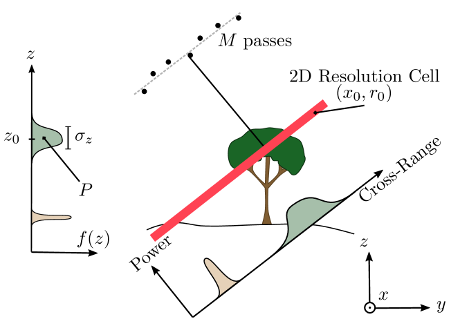
Figure 1: SAR Tomography principle.

A tomographic SAR measurement, illustrated in Figure 1, consists of $M$ 2D SAR acquisitions performed from slightly shifted, and ideally parallel, tracks. Under the widely accepted first order Born approximation, considering that the echoes of individual scatterers sum up to form the response a scene, the expression of one of the 2D SAR images of a general 3D environement may be written as:

$$s_{m}(x_{0},r_{0})=\int h(x-x_{0},r-r_{0})a_{c}(\mathbf{r})\text{e}^{jk_{c}r}d\mathbf{r}+\epsilon_{m}(x_{0},r_{0}),$$ (1)

where $r_{0}$ and $x_{0}$ stand for the range and azimuth coordinates of the images, respectively, $h(x,r)$ is the 2D SAR ambiguity function, $k_{c}$ is the carrier two-way wavenumber, $\bm{r}$ is a 3D coordinate, and $r$ is its associated range, i.e., the orthogonal distance between the flight track and location $\bm{r}$, $\epsilon_{m}(x_{0},r_{0})$ is the normally distributed focused acquisition noise, and $a_{c}(\bm{r})$ represents the coherent density of scattering of the scene. Over natural environments, this density, consisting of a large number of independent contributions originating from randomly distributed sources, is usually assumed to follow a complex circular normal distribution verifying $\mathrm{E}[a_{c}(\mathbf{r})]=0$, $\mathrm{E}[a_{c}(\mathbf{r})a_{c}(\mathbf{r}+d\mathbf{r})]=0$, and $\mathrm{E}[a_{c}(\mathbf{r})a_{c}^{*}(\mathbf{r}+d\mathbf{r})]=\sigma_{a}^{2}(\mathbf{r})\delta(d\mathbf{r})$ with $\sigma_{a}^{2}(\mathbf{r})$, the 3D density of reflectivity of the scene.

The ambiguity associated with 2D SAR imaging may be perceived in (1), with a cylindrical projection the 3D scattering density onto a 2D range-azimuth domain. SAR tomography proposes to overcome this limitation using spatial diversity and coherent array processing. To do so, the $M$ SAR images are coregistered to a reference geometric frame, and are demodulated to the spatial baseband domain. The resulting tomographic image stack, $\mathbf{y}(x_{0},r_{0})\in\mathbb{C}^{M}$ follows a centered complex circular distribution, $\mathbf{y}\sim\mathcal{CN}(\mathbf{0},\mathbf{R})$, whose second order statistics can be used to retrieved 3D reflectivity features. In the case of a horizontally homogeneous environment, i.e., when the 2D ambiguity function is narrow enough so that the scattering density at a given elevation may be considered as stationary within a 2D resolution cell, the expression of the interferometric cross-correlation simplifies to:

$$\mathrm{E}[y_{n}y_{m}^{*}]=\int f(z)\text{e}^{jk_{z_{nm}}z}dz+\sigma_{\varepsilon}^{2}\delta(n-m),$$ (2)

where the range and azimuth coordinates of the concerned 2D resolution cell have been omitted for the sake of clarity, and $f(z)$, the vertical component of $\sigma_{a}^{2}(\mathbf{r})$, represents the vertical density of reflectivity. The relationship between the elevation of a contributing source and the interferometric phase of its response is given by $k_{z_{nm}}=k_{z_{n}}-k_{z_{m}}$, with $k_{z_{n}}$ the interferometric wave number of the n^th image. The vertical Fourier resolution is given by $\delta z=2\pi/(\max_{n}k_{z_{n}}-\min_{n}k_{z_{n}})$, whereas the vertical ambiguity may be approximated, for a quasi-uniform wave number spacing, as $z_{amb}\approx M\delta z$.

II-B Covariance matrix model

The tomographic cross-correlation expression of (2) may be generalized using antenna array processing formalism. The covariance matrix of the tomographic acquisition can be formulated as:

$$\bm{R}\triangleq\mathrm{E}[\bm{y}\bm{y}^{H}]=P\int p(\omega-\omega_{0})\bm{a}(\omega)\bm{a}(\omega)^{H}\,d\omega+\sigma_{\varepsilon}^{2}\bm{I}_{M}.$$ (3)

where $\omega_{0}$ denotes the mean spatial frequency, $P$ the power of the source, $p$ its distribution around $\omega_{0}$ which satisfies $\int p(\omega)\,d\omega=1$ and $\int\omega p(\omega)\,d\omega=0$, and $\bm{a}(\omega)$ is a steering vector expressed as:

$$\bm{a}(\omega)\triangleq\begin{pmatrix}1&e^{j2\pi u_{2}\omega}&\cdots&e^{j2\pi u_{M}\omega}\end{pmatrix}^{\intercal}\in\mathbb{C}^{M}.$$ (4)

In (4), $u_{k}$ denotes the distance (in wavelength) between the first and the $k$^th element in the equivalent linear array, and $\omega=\sin\phi$, with $\phi$ the associated angle of arrival on the array. The expression of $\bm{R}$, (3), may be reformulated as:

$$\bm{R}=\bm{a}(\omega_{0})\bm{a}^{H}(\omega_{0})\odot P\bm{B}+\sigma_{\epsilon}^{2}\bm{I}_{M},$$ (5a)

where $$\odot \bm{B} (k,l)$$ denotes the Hadamard (element-wise) matrix product, and is a form matrix that depends on the scattering distribution. Its entry is:

$$\left[{\bm{B}}\right]_{k,l}\triangleq\int p(\tilde{\omega})e^{j2\pi(u_{k}-u_{l})\tilde{\omega}}\,d\tilde{\omega},$$ (5b)

where $\tilde{\omega}\triangleq\omega-\omega_{0}$. The objective of the analysis is to estimate, from the covariance matrix of the observations $\left\{\bm{y}\right\}$, three characteristics of the power density of the distributed source: $(i)$ its mean spatial frequency $\omega_{0}$, $(ii)$ its standard deviation $\sigma_{\omega}$, and $(iii)$ its power $P$. In the context of forest SAR tomography, they correspond to the height $z_{0}$ of the forest canopy, its thickness $\sigma_{z}$, and its reflectivity $P$ as illustrated in Figure 1.

III Proposed estimation scheme

III-A COMET estimator

The COMET estimator [10] is used to estimate the characteristics of the source. It is based on a generalized least squares method, and represents an efficient alternative to the Maximum Likelihood estimator of the unconditional model at hand [4]. If the covariance matrix is parameterized by some vector $\bm{\theta}$ as $\bm{\hat{R}}(\bm{\theta})$, the COMET estimate is obtained by minimizing the following cost function:

$$J(\bm{\theta})=\left\lVert\bm{W}^{H/2}(\bm{\bar{R}}-\bm{\hat{R}}(\bm{\theta}))\bm{W}^{1/2}\right\rVert^{2},$$ (6)

where $\bm{\bar{R}}\triangleq\frac{1}{N}\sum_{t=1}^{N}\bm{y}(t)\bm{y}(t)^{H}$ is the sample covariance matrix, $\bm{y}(t)$ is a realization of $\bm{y}$, and $\bm{W}$ is a Hermitian weight matrix. Two choices of weight matrix are commonly used: $\bm{W}=\bm{I}$ which corresponds to an unweighted least square method, and $\bm{W}=\bm{\bar{R}}^{-1}$ which is proved to induce an asymptotically efficient estimator if the model $\bm{\hat{R}}(\bm{\theta})$ is correctly specified [10]. Before applying the COMET estimator, a model should be chosen for the estimated matrix $\bm{\hat{R}}(\bm{\theta})$.

III-B Moment-based model

The difficulty in modeling the covariance matrix $\bm{R}$ comes from the fact that the scatterer distribution $p$ is unknown. The entries of the matrices $\bm{R}$ and $\bm{B}$ are not directly related to the distribution $p$, but to its Fourier Transform (FT) $\widehat{p}$, described here using a non-parametric model. Assuming that the scatterer distribution is narrow, the FT spreads over a large domain, and is very smooth at $0$. Therefore, ${\widehat{p}}$ can be accurately approximated near the origin by the first terms of its Taylor expansion, and represents, by definition, the characteristic function of the distribution. These coefficients correspond, up to a factor, to the central moments of the distribution. Let $\mu_{d}$ denote the $d$-th central moment of the distribution, $\mu_{d}\triangleq\mathrm{E}[\tilde{\omega}^{d}]$, then $\mu_{0}=1$ and $\mu_{1}=0$. It is proposed to parameterize $\widehat{p}$ by its first $D$ central moments, the choice of the order $D$ being discussed in Section IV. For a vector $\bm{\mu}=\begin{pmatrix}\mu_{2}&\cdots&\mu_{D}\end{pmatrix}^{\intercal}\in\mathbb{R}^{D-1}$, the FT $\xi\mapsto\widehat{p}(\xi)$ is approximated by:

$$\widehat{p}(\xi,\bm{\mu})=1+\sum_{d=2}^{D}\frac{j^{d}}{d!}\mu_{d}\xi^{d}.$$ (7)

Such a parameterization has two main advantages. First, it does not assume any scatterer distribution model, which would lead to a loss of accuracy in the case of an incorrect specification, as illustrated in Section IV. Second, the central moment $\mu_{2}\triangleq\sigma_{\omega}^{2}$ corresponds to the dispersion of the distribution to be estimated.

The parametrization (7) induces the following model for the matrices $\bm{B}$ and $\bm{R}$:

$$\bm{\hat{B}}(\bm{\mu}) =\bm{1}\bm{1}^{\intercal}+\sum_{d=2}^{D}\frac{j^{d}}{d!}\mu_{d}\bm{U}^{(d)},$$ (8a)

$$\bm{\hat{R}}(\bm{\theta}) =\bm{a}(\omega_{0})\bm{a}(\omega_{0})^{H}\odot P\bm{\hat{B}}(\bm{\mu})+\sigma_{\varepsilon}^{2}\bm{I}_{M},$$ (8b)

where the parameter vector is $\bm{\theta}\triangleq\left(\omega_{0},\,P,\,\sigma_{\varepsilon}^{2},\,\bm{\mu}^{\intercal}\right)^{\intercal}\in\mathbb{R}^{D+2}$, and the matrices $\bm{U}^{(d)}$ depend only on the geometry of the array. Its $(k,l)$ entry is $\left[{\bm{U}^{(d)}}\right]_{k,l}=(u_{k}-u_{l})^{d}$. In particular, this parametrization is also valid for non-uniform arrays.

III-C Estimation algorithm

Before applying the COMET estimation scheme, a transparent modification is made in the parameter vector to ease the optimization. The vector $\bm{\nu}\triangleq P\bm{\mu}$ is used to define the parameter vector $\bm{\theta}\triangleq\left(\omega_{0},\,P,\,\sigma_{\varepsilon}^{2},\,\bm{\nu}^{\intercal}\right)^{\intercal}\in\mathbb{R}^{D+2}$. This change of variable makes the dependence of $\bm{\hat{R}}$ linear on all the parameters, except $\omega_{0}$. Note that as $P>0$, this change of variable is invertible.

Denote, as in [10], $\bm{\alpha}\triangleq\left(P,\sigma_{\varepsilon}^{2},\bm{\nu}^{\intercal}\right)^{\intercal}\in\mathbb{R}^{D+1}$ the set of linear parameters in $\bm{\theta}$. The cost function $J$, (6), can be re-expressed in vector form as:

$$J(\omega_{0},\bm{\alpha})=(\bm{\bar{r}}-\bm{\Psi}(\omega_{0})\bm{J}\bm{\alpha})^{H}\left(\bm{W}^{\intercal}\otimes\bm{W}\right)(\bm{\bar{r}}-\bm{\Psi}(\omega)\bm{J}\bm{\alpha}),$$ (9)

where $\bm{\bar{r}}\triangleq\operatorname*{\mathrm{vec}}\bm{\bar{R}}$ is the vector obtained by stacking the columns of $\bm{\bar{R}}$, $\otimes$ denotes the Kronecker matrix product, $\bm{J}$ is the matrix such that $\operatorname*{\mathrm{vec}}\left\{P\bm{B}(\mu)+\sigma_{\varepsilon}^{2}\bm{I}_{M}\right\}=\bm{J}\bm{\alpha}$, and:

$$\bm{\Phi}(\omega) \triangleq\operatorname{\mathrm{diag}}\bm{a}(\omega), \bm{\Psi}(\omega) \triangleq\bm{\Phi}(\omega)^{H}\otimes\bm{\Phi}(\omega).$$

As pointed out in [10], for any set $\omega_{0}$ value, (3) is a quadratic form in $\bm{\alpha}$ whose minimum is achieved at:

$$\bm{\hat{\alpha}}(\omega_{0})=\left[(\bm{\Psi}(\omega_{0})\bm{J})^{H}(\bm{W}^{\intercal}\otimes\bm{W})(\bm{\Psi}(\omega_{0})\bm{J})\right]^{-1}\\ \times\bm{\Psi}(\omega_{0})\bm{J})^{H}(\bm{W}^{\intercal}\otimes\bm{W})\bm{\bar{r}}.$$ (10)

Thus, a single optimization on $\omega_{0}$ is required to find the minimizer of $J$. By re-injecting (10) in $J$, one obtains:

$$\hat{\omega}_{0}=\arg\max\bm{y}(\omega)^{H}\bm{Y}(\omega)^{-1}\bm{y}(\omega),$$ (11)

with:

$$\bm{y}(\omega) \triangleq(\bm{\Psi}(\omega)\bm{J})^{H}(\bm{W}^{\intercal}\otimes\bm{W})\bm{\bar{r}},$$

$$\bm{Y}(\omega) \triangleq(\bm{\Psi}(\omega)\bm{J})^{H}(\bm{W}^{\intercal}\otimes\bm{W})\bm{\Psi}(\omega)\bm{J}.$$

The one-dimensional optimization problem in (11) can be solved with a linear search or a golden-section search. Once, $\hat{\omega}_{0}$ has been estimated, all the other parameters can be derived. The full estimation algorithm is summarized in Algorithm 1.

Algorithm 1 Estimation algorithm.

1:Form the sample covariance matrix $\bm{\bar{R}}$ from the measurements $\left\{\bm{y}\right\}$.

2:Estimate $\hat{\omega}_{0}$ by solving the one-dimensional optimization problem (11).

3:Compute $\hat{P}$, $\hat{\sigma}_{\varepsilon}$, and $\bm{\hat{\nu}}$ from (10) with $\omega_{0}=\hat{\omega}_{0}$.

4:Compute the estimates of the central moments as: $\hat{\mu}=\hat{\nu}/\hat{P}$. In particular, $\hat{\sigma}_{\omega}^{2}=\hat{\mu}_{2}$.

IV Numerical simulations

This section presents numerical simulations to demonstrate the efficiency of the proposed approach. The simulation scenario illustrates a typical SAR tomography configuration. The observed scene corresponds to a forest whose ground response has been canceled out using a notching preprocessing step [11]. Unless otherwise stated the selected configuration is characterized by its height ambiguity $z_{amb}=100$ m, its vertical resolution $\delta z\approx 14.3$ m, canopy thickness $\sigma_{z}$ of $5$ m, and number of acquisitions $M=7$, which are typical settings for forest SAR tomography [3]. The weight matrix is fixed to $\bm{W}=\bm{\bar{R}}^{-1}$.

IV-A Influence of the order $D$

(a)

(b)

(c)

Figure 2: RMSE for different orders $D$ and different (Gaussian and exponential) distribution shapes. The simulation parameters are $\sigma_{z}=5$ m, $SNR=P/\sigma_{\varepsilon}^{2}=20$ dB, $M=7$ sensors ($D_{\text{max}}=11$), $\delta z\approx 14.3$ m. The RMSE estimates were computed over $5\ 000$ realizations

The possible values of $D$ are constrained by the size of the array. With an $M$-sensor array, the covariance matrix $\bm{R}$ has up to $M(M-1)+1$ different entries. This number is reduced to only $2M-1$ in the case of a uniform array. The number of parameters in $\bm{\theta}$ must be smaller than the number of observables to ensure the solvability of the problem. Therefore, the maximum value of $D$ is:

$$D_{\mathrm{max}}=\left\{\begin{array}[]{cl}2M-3&\text{for a uniform array,}\\ M(M-1)-1&\text{for a general array.}\end{array}\right.$$ (12)

Thus, the hyper-parameter ${D}$ must satisfy $2\leq D\leq D_{\mathrm{max}}$. In particular, identifying the dispersion of the source $\sigma_{\omega}$, requires at least $M=3$ sensors.

A natural question is then, should ${D}$ be set to its maximum possible value? Conceptually, the moment-based estimation scheme is a polynomial interpolation of the characteristic function of the scatterer distribution, and $D$ corresponds to the order of interpolation. On the one hand, large orders allow to capture more complex functions. However, large orders also increase the risk of overfitting the data and oscillations, due to Runge’s phenomenon. In the context of SAR tomography, the number of sensors $M$ is small, typically $7$ at most, and these two phenomena hardly occur. Hence, larger $D$ values provide better accuracy. Figure 2 shows the evolution of the Root Mean Square Error (RMSE) on the estimates as a function of the number of snapshots $N$ and of the order $D$. A clear gain of performance is obtained as the order increases. It is important to note that the maximum order achieves similar accuracy with two very different, Gaussian and Exponential, distribution shapes. This confirms that the proposed approach is independent of the true distribution, and in particular, that it works similarly with symmetric and asymmetric distributions.

IV-B Comparison with parametric schemes

(a)

(b)

(c)

Figure 3: RMSE on the estimation of a uniform distributed source for different estimation schemes: ML estimators under three different distribution assumptions (“Gaussian”, “Exponential” and “Uniform”), the proposed approach with $D=D_{\text{max}}$ (“No assumption”), and its adaptation to symmetric distributions (“Symmetric”). The same configuration as in Fig. 2 is used.

(a)

(b)

(c)

Figure 4: RMSE as a function of the source spread $\sigma_{z}$. The same configuration as in Fig. 3 is used, the number of snapshots is set to $N=100$. For large $\sigma_{z}$ values, the misspecified ML algorithms did not converge.

The proposed approach is compared with parametric methods. Figure 3 presents RMSE values for different estimation schemes. The proposed algorithm is compared with parametric ML estimators, specified under different scattering distribution assumptions, and applied onto data generated using a uniform distribution. The ML estimators are computed under the assumption of a Gaussian, exponential, and uniform distribution. As expected, the best performing method is the ML estimator with the correct distribution assumption. For the estimation of $\omega_{0}$, the ML estimator with the Gaussian assumption also performs better than our scheme. This due to the fact that both the Gaussian and uniform shapes represent symmetric distributions. On the other hand, the exponential assumption, which is asymmetric, yields biased results: asymmetry induces a bias in the estimation of $\omega_{0}$. The proposed scheme is easily adapted to impose the symmetry of the distribution by considering only the even orders. Figure 3 also shows the RMSE obtained with this adaptation which is, as expected, more accurate for estimating $\omega_{0}$. For the estimation of the dispersion $\sigma_{\omega}$ and the power $P$, the two incorrect assumptions lead to biased estimates and are outperformed by the proposed algorithm.

The proposed scheme is based on a approximation of the FT $\widehat{p}$ by the first terms of its Taylor expansion at $0$. Such an approximation is only valid if $\widehat{p}$ is sufficiently regular in the neighborhood of 0, i.e., if the distribution $p$ is sufficiently narrow. If the dispersion $\sigma_{z}$ is too large, this approximation is no longer valid. Figure 4 compares the performance of the schemes as a function of $\sigma_{z}$. As before, it can be noted that the proposed scheme outperforms the misspecified ML estimators over a wide range of values. For large dispersion, when $\sigma_{z}$ is larger than the resolution $\delta z\approx 14.3$ m, the performance of the moment-based algorithm decreases as expected. For small dispersions, the proposed approach also produces poor results, worse than the misspecified ML estimators. There are two reasons for this: first, when the dispersion is much smaller than the resolution, two different distributions become hard to distinguish, and second, the proposed scheme requires a larger number of snapshots. With more snapshots, the proposed approach would improve its estimates, while the misspecified ML estimators would converge to biased estimates.

V Concluding remarks

This paper presents a new method for estimating the characteristics of a spatially distributed scattering source. The proposed approach does not assume any distribution for the scatterers, but relies on the estimation of the central moments of their distribution. When applied to a SAR tomography scenario, it allows to efficiently estimate the location of the source, its power, and its dispersion without assuming a distribution model, which would introduce estimation biases. A second point relevant to SAR tomography applications is that the proposed approach does not require a uniform linear array and can be applied with irregular baselines. Conceptually, the moment-based estimation presented in this work is a polynomial interpolation of the characteristic function of the distribution. As a consequence, it is computationally efficient: the algorithm requires only a single one-dimensional search. However, it may suffer from the problems of overfitting or oscillations as the resolution increases, i.e., as $M$ increases. These problems are not encountered in the context of SAR tomography, but they should be further investigated in future work. Another avenue should be the joint estimation of multiple scatterers sources, whether diffuse or point sources.

References

- [1] H. Aghababaei, G. Ferraioli, L. Ferro-Famil, Y. Huang, M. Mariotti D’Alessandro, V. Pascazio, G. Schirinzi, and S. Tebaldini, “Forest SAR tomography: Principles and applications,” IEEE Geoscience and Remote Sensing Magazine, vol. 8, no. 2, pp. 30–45, 2020.
- [2] F. Gini and F. Lombardini, “Multibaseline cross-track SAR interferometry: a signal processing perspective,” IEEE Aerospace and Electronic Systems Magazine, vol. 20, no. 8, pp. 71–93, 2005.
- [3] P.-A. Bou, L. Ferro-Famil, F. Brigui, and Y. Huang, “Tropical forest characterisation using parametric SAR tomography at P band and low-dimensional models,” IEEE Geoscience and Remote Sensing Letters, pp. 1–1, 2024.
- [4] P. Stoica and A. Nehorai, “Performance study of conditional and unconditional direction-of-arrival estimation,” IEEE Transactions on Acoustics, Speech, and Signal Processing, vol. 38, no. 10, pp. 1783–1795, 1990.
- [5] O. Besson and P. Stoica, “Decoupled estimation of DOA and angular spread for a spatially distributed source,” IEEE Transactions on Signal Processing, vol. 48, no. 7, pp. 1872–1882, 2000.
- [6] A. Zoubir, Y. Wang, and P. Chargé, “A modified COMET-EXIP method for estimating a scattered source,” Signal Processing, vol. 86, no. 4, pp. 733–743, 2006.
- [7] S. Shahbazpanahi, S. Valaee, and A. Gershman, “A covariance fitting approach to parametric localization of multiple incoherently distributed sources,” IEEE Transactions on Signal Processing, vol. 52, no. 3, pp. 592–600, 2004.
- [8] S. Valaee, B. Champagne, and P. Kabal, “Parametric localization of distributed sources,” IEEE Transactions on Signal Processing, vol. 43, no. 9, pp. 2144–2153, 1995.
- [9] S. Shahbazpanahi, S. Valaee, and M. Bastani, “Distributed source localization using ESPRIT algorithm,” IEEE Transactions on Signal Processing, vol. 49, no. 10, pp. 2169–2178, 2001.
- [10] O. Ottersten, P. Stoica, and R. Roy, “Covariance matching estimation techniques for array signal processing applications,” Digital Signal Processing, vol. 8, no. 3, pp. 185–210, 1998.
- [11] M. Mariotti d’Alessandro, S. Tebaldini, S. Quegan, M. J. Soja, L. M. H. Ulander, and K. Scipal, “Interferometric ground cancellation for above ground biomass estimation,” IEEE Transactions on Geoscience and Remote Sensing, vol. 58, no. 9, pp. 6410–6419, 2020.