Tunable topological protection in Rydberg lattices via a novel quantum Monte Carlo approach

Abstract

Rydberg atom arrays have recently been conjectured to host $Z_{2}$ quantum spin liquids (QSLs) in certain parameter regimes. Due to the strong interactions between these atoms, it is not possible to analytically study these systems, and one must resort to Monte Carlo sampling of the path integral to reach definite conclusions. We use a tailored update, specifically designed to target the low energy excitations of the QSL. This allows us to reliably simulate Rydberg atoms on a triangular lattice in the proposed QSL regime. We identify a correlated paramagnetic phase at low temperatures which hosts topological protection similar to a $Z_{2}$ spin liquid up to a length scale tuned by Hamiltonian parameters. However, this correlated paramagnet seems to be continuously connected to the trivial paramagnetic regime and thus does not seem to be a true QSL. This result indicates the feasibility of Rydberg atom arrays to act as topological qubits.

Rydberg atom arrays have recently emerged as powerful platforms to simulate quantum many-body systems Jaksch et al. (2000); Lukin et al. (2001); Urban et al. (2009); Browaeys and Lahaye (2020). The high degree of control generated by optical traps and laser detuning allows the realization of simple models which may host entangled ground states. One of the simplest models which approximate the behavior of such arrays to a high degree is the PXP model Bluvstein et al. (2021); Pan and Zhai (2022); Chen and Iadecola (2021), which encodes the Coulomb repulsion between the large electron clouds of neighboring excited atoms as a simple exclusion rule which prevents co-existing excitations. It has been suggested Verresen et al. (2021); Samajdar et al. (2021); Yan et al. (2022) that atoms on triangular and Kagomé lattices can realize a $Z_{2}$ quantum spin liquid. Experiment evidence also supports this proposal Semeghini et al. (2021). Such a state is not only of interest from a theoretical perspectiveZhou et al. (2017); Savary and Balents (2016), but also serves as the cornerstone for topologically protected quantum computingKitaev (2003).

The strong correlations inherent to the PXP model make it prohibitively difficult to understand the behavior of the system analytically. Thus, density matrix renormalization group (DMRG) simulations have been used to show the presence of a QSL in a PXP model defined on the links of a Kagomé lattice Verresen et al. (2021). However, due to the nature of the method, these studies have been limited to the ground state and to pseudo-1D geometries.

Quantum Monte Carlo (QMC) simulations have also been employed to simulate a quantum dimer model with added terms to emulate the PXP Hamiltonian, and these have shown that it is possible to achieve QSL phases in the phase diagram of such a modelYan et al. (2022) on the links of a triangular lattice. However, the mapping from the PXP model to a quantum dimer model(QDM) is approximate, and it is not clear how applicable the results are to the original model. In this Article, we will address that issue by applying QMC simulations to the PXP model on the triangular lattice. To enable this, we have developed a novel Monte Carlo update which makes of intuition derived from QDM studies. For QDMs with built-in resonating terms, a novel update called the sweeping cluster algorithm has been used Yan et al. (2019); Yan (2022) to efficiently sample the configuration space in the corresponding QMC simulation. As the PXP model does not explicitly have such a resonance term, we have developed here an update which identifies the resonances emergent at low temperature, and utilize a sampling which toggles between various resonances, just as expected for a QSL. Although there already exist local and cluster algorithms for the PXP and similar models for Rydberg atoms Merali et al. (2021); Yue et al. (2021); Yan et al. (2019); Biswas et al. (2016); Hearth et al. (2022); Wu et al. (2023, 2021), we explicitly show that the resonance update is crucial for efficient sampling in the proposed QSL regime. This algorithm can be easily generalized to other model Hamiltonians which may host QSL physics, and is expected to provide a significant improvement in sampling efficiency. We use our algorithm to show the presence of a correlated paramagnet which resembles a QSL at small scale in the PXP model on the triangular lattice, but which seems to be smoothly connected to a trivial paramagnetic phase, even at zero temperature.

Figure 1: Zero temperature phase diagram for the $PXP$ model on the triangular lattice as a function of the strength of quantum fluctuations $\Omega$. Strictly at $\Omega=0$, the ground state is a $Z_{2}$ classical spin liquid (CSL) which has short-ranged correlations. For small $\Omega$, comparisons with the quantum dimer model suggest the appearance of a $\sqrt{12}\times\sqrt{12}$ ordering Moessner and Sondhi (2001). We have investigated the ground state for $\Omega>0.4$ and find a correlated paramagnet (CP) which exhibits behavior consistent with a $Z_{2}$ QSL up to intermediate system sizes, followed by a simple quantum paramagnet (QP) for large $\Omega$.

The central numerical results which we are able to achieve using the algorithm described above can be summarized as follows : Fredenhagen-Marcu order parameters Fredenhagen and Marcu (1983); Xu et al. , which are used to identify topological ordering in dilute dimer models, show a parameter regime which is consistent with a $Z_{2}$ QSL. In addition, the dimer and energy densities show changes in behavior consistent with a transition between two phases as a function of the control parameter. However, these changes do not sharpen into non-analyticities with increasing size (as expected at a phase transition) and the energy density as a function of temperature reveals a finite gap in the large size limit, with no indication of a gap closing on the phase diagram. Since the simulations are carried out at temperatures substantially below the measured excitation gap, and since calculations of the entropy reveal that we reach the ground state regime, we do not believe that the smooth crossover from the correlated to trivial paramagnet is only a matter of finite temperature. Rather, we conclude that in the parameter regime we have been able to analyze, there exists only a correlated paramagnetic ground state (Fig. 1), which behaves similarly to a $Z_{2}$ QSL for intermediate system sizes but is not a true QSL.

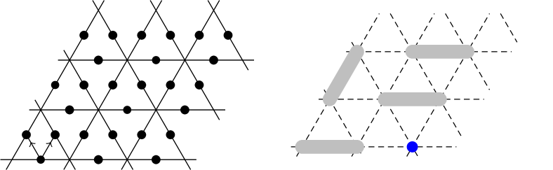
Figure 2: (Left) Rydberg atoms living on the links of a triangular lattice. Each upward pointing triangle is a unit cell, and the vectors within a unit cell used to define the structure factor (Eq. (5)) are shown for the first cell. (Right) Excitations can be seen as dimers occupying the relevant links. For a $3\times 3$ lattice, there is an odd number of lattice sites, and thus there must be at least one site not covered by a dimer.

I Model and formulation of SSEQMC

The most common modelVerresen et al. (2021); Yan et al. (2023) for Rydberg atom arrays is given by hard-core bosons with a strong repulsive interaction and a kinetic term which creates/annihilates bosons. In the limit of infinite repulsion, the kinetic term can act only if every neighboring location is empty. This reduces to the PXP model Turner et al. (2018), where the P stands for a projection operator which enforces zero occupancy on the required locations, and $X$ denotes a transverse field in spin language ($b+b^{\dagger}$ in boson language). We define our system on a triangular lattice with $L^{2}$ sites ($N=3L^{2}$ links), where $L$ is the linear dimension of the system (this can be seen as a 2D version of the model studied in Ref. Fendley et al. (2004)). The Rydberg atoms are placed at the link centers as shown in Fig. 2. For ease of comparison we begin with the paradigmatic Hamiltonian for Rydberg atom arrays, parameterized in the same way as Ref. Verresen et al. (2021) :

$$H=\frac{\Omega}{2}\sum_{i}(b_{i}+b_{i}^{\dagger})-\delta\sum_{i}n_{i}+\frac{1}{2}\sum_{i,j}V(|i-j|)n_{i}n_{j}.$$ (1)

The Coulomb repulsion due to the Rydberg blockade is encoded in $V(|i-j|)$, which is known to have the functional form $V(r)\sim 1/r^{6}$ Urban et al. (2009). As this is extremely short range, we make the approximation that for nearest neighbors $V(r)\to\infty$, and $V(r)=0$ otherwise. This provides us with the effective PXP model discussed above. We have effectively removed all states from our boson occupation basis which have bosons on nearest neighbors. Within this restricted space, the Hamiltonian simply reduces to

$$H=\frac{\Omega}{2}\sum_{i}(b_{i}+b_{i}^{\dagger})-\delta\sum_{i}n_{i}.$$ (2)

It is important to note here that even though it is not apparent from Eq. (2), the restricted Hilbert space renders the system genuinely interacting. As there is a freedom of one energy scale, we set $\delta=1$ for all our numerical results, unless otherwise mentioned.

We can also express this as a spin model, using the mapping between hard-core bosons and spin-1/2 operators: $b_{i}^{\dagger}\to\sigma_{i}^{+};\ b_{i}\to\sigma_{i}^{-};n_{i}\to\frac{1}{2}(\sigma^{z}_{i}+1).$

In the spin language the Hamiltonian takes the form of non-interacting spins in a global tilted field (up to constant terms):

$$H=\frac{\Omega}{2}\sum_{i}\sigma^{x}_{i}-\frac{\delta}{2}\sum_{i}\sigma^{z}_{i}$$ (3)

However, it is worth noting here again that due to the restricted Hilbert space allowed by the Rydberg constraint, the spins should be considered to be strongly interacting, and thus capable of interesting many-body physics.

In the restricted space, the action of the chemical potential is to maximize the density of bosons, thus leading to fully packed configurations with no neighboring locations simultaneously occupied by bosons. In contrast, the kinetic term acts by creating resonances between the occupied and unoccupied state, and in many cases leads to a phase continuously connected to the trivial $x$-polarized paramagnet one would expect in the limit of large transverse field.

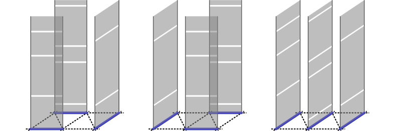
Figure 3: Path integral configurations in the classical spin liquid regimes. Quantum fluctuations can be seen as breaks in the imaginary time direction, and do not produce non-trivial structural changes.

A spin liquid ground state may be realized by placing Rydberg atoms on the links of the triangular lattice, as shown in Fig. 2. The Rydberg constraint then excludes a simultaneous excitation of two links which share a vertex. Although the constraint does not function exactly in this manner for the native Rydberg models, it has recently been shown that Rydberg “gadgets” can be built into the experimental set-up to realize the dimer model accuratelyZeng et al. (2024). This makes the system similar to a hard core dimer model, where a Rydberg excitation can be understood as a dimer living on the corresponding link, a Rydberg ground state as the absence of a dimer, and the exclusion requirement now implies that two dimers do not share an end point. In the classical limit $\Omega=0$, the system now hosts a degenerate set of all fully packed dimer coverings as its ground state, where the fully packed requirement comes from the chemical potential term controlled by $\delta$. This suggests that for $\Omega\ll\delta$, it may be possible to generate superpositions of these dimer coverings, and thus a $Z_{2}$ spin liquid.

I.1 SSEQMC to path integral configurations

QMC involves sampling of path integral configurations which can be understood from the Trotter decomposition of the partition function $Z=Tr[e^{-\beta H}]$. Writing $e^{-\beta H}=(e^{-\Delta\tau H})^{n}$, and inserting a complete basis after each $e^{-\Delta\tau H}$ leads to configurations defined by a collection of basis states $\{\alpha_{0},\alpha_{1}...\alpha_{n-1}\}$ (where $\alpha_{i}$ denotes a product state in our local basis), and this set is usually stacked vertically in the third dimension to visualize a path integral configuration.

For our simulations, we use quantum Monte Carlo simulations in the stochastic series expansion formalism (SSEQMC) Sandvik (1992). In our case, the first step in this formalism involves writing the Hamiltonian as a sum of local terms $H=h_{1}+h_{2}+..+h_{m}$, which do not have a branching property, i.e. $h_{k}\ket{i}=c^{i}_{k}\ket{j}$, where $\ket{i}$ and $\ket{j}$ are product states, and the set $\{c^{i}_{k}\}$ form the corresponding numerical coefficients. Thus each $h_{k}$ is a bijective map from a product state to another product state in our chosen basis. For the next step, we expand the partition function, $Z=Tr[e^{-\beta H}]$, as $\sum_{n}\frac{(-\beta)^{n}}{n!}\sum_{s_{n}}Tr[h_{s^{1}_{n}}h_{s^{2}_{n}}...h_{s^{n}_{n}}]$, where $s_{n}$ denotes a string of size $n$ and specifies the local terms participating in the specific series of interest. As a final step to help us visualize these strings as path integral configurations, we insert complete basis sets in the boson occupation basis (denoted by $\sum_{\alpha}\ket{\alpha}\bra{\alpha}$) between each pair $h_{s^{m}_{n}}h_{s^{m+1}_{n}}$ and for the trace. Due to the non-branching property discussed above, only the sum over the basis set for the trace remains. We denote this by $\sum_{\alpha_{0}}\ket{\alpha_{0}}\bra{\alpha_{0}}$, and for a fixed $\alpha_{0}$ and particular $s_{n}$, all the intermediate basis states are specified as $h_{s^{1}_{n}}\ket{\alpha_{0}}$ returns a unique basis state, $h_{s^{2}_{n}}$ acting on that state again returns a unique basis state and so on. We denote the intermediate states by $\ket{\alpha_{1}},\ket{\alpha_{2}}..\ket{\alpha_{n-1}}$. Each state is represented by a dimer covering on the triangular lattice, and we denote the collection of states $\{\ket{\alpha_{0}},\ket{\alpha_{1}},\ket{\alpha_{2}}...\}$ as a path integral configuration by stacking them vertically in sequence. This creates a three-dimensional configuration (as shown in Figs. 3 and  4); identical configurations are also generated by carrying out a vanilla Trotter decomposition of $Tr[e^{-\beta H}]$, and the vertical dimension is usually referred to as the imaginary time direction.

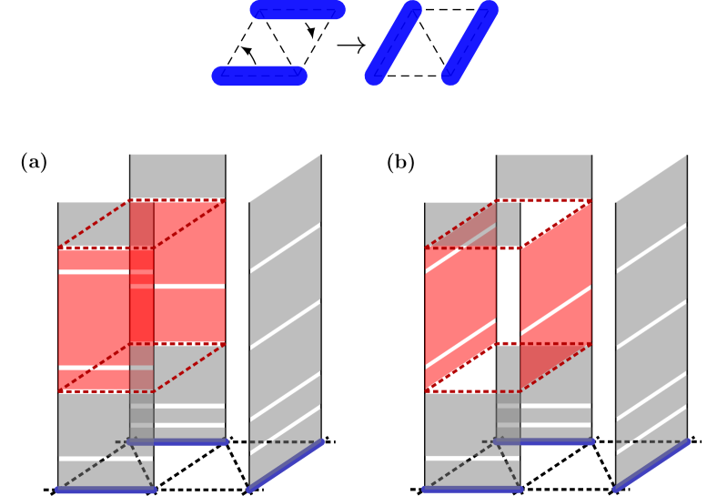
Figure 4: (Top) Two-dimer resonance on the triangular lattice. (a) and (b) path integral configurations which contribute to the partition function, related by the resonance shown above.

II Path integral configurations

To motivate the sampling algorithm which we use in our Monte Carlo simulation, we discuss the possible path integral configurations which dominate the partition function of classical and quantum spin liquids.

Let us begin now with the purely classical limit $\Omega=0$. As all individual terms in the Hamiltonian are now diagonal, all basis states in a path integral configuration must be identical (as $\braket{a^{1}|H|a^{2}}=0$ if $\ket{a^{1}}\neq\ket{a^{2}}$). Thus the configuration can be simply imagined as a single fully packed dimer covering extended into the time dimension. The quantum fluctuation which we introduce for non-zero $\Omega$ acts on a single link by either destroying or creating a dimer. For small $\Omega$, the effect of this on the path integral configurations can be understood as small segments of dimer absence which appear as breaks in the otherwise continuous dimer world line which we expect in the classical limit. Cartoons for this type of configuration are shown in Fig. 3. The ensemble of path integral configurations still retains its classical signature in this limit, and various configurations can be generated by taking different dimer coverings, drawing them out in the time direction, and populating them with the small breaks generated by the quantum fluctuation. These configurations are expected in the $\Omega\ll\delta$ limit, and are shown in Fig. 3. The inverse temperature $\beta$ sets the length scale for the imaginary time direction, and plays an important role here, as it controls how many breaks are allowed in a particular configuration. Naively, the size and density of the breaks would be expected to be independent of size of the system in both space and time.

For the cartoon picture of a classical spin liquid discussed here, the basis states in a particular path integral configuration are more or less perfectly correlated. For a quantum spin liquid, this would not be the case, as we should expect events in imaginary time which resemble resonances between different dimer coverings. Examples of two and three dimer resonances on the triangular lattice are shown in Fig. 4. In the path integral representation, these events can occur if there are coordinated breaks on links which are compatible with a resonance. For $\Omega\approx O(\delta)$, this is statistically likely, and this event manifests in the path integral configuration as a sudden resonance with a short span in imaginary time. Due to the trace condition, the resonance should undo itself as a later point in imaginary time, thus leading to a pair of resonances. A cartoon for such a configuration is shown in Fig. 4, along with the configuration generated by flipping the column between the resonances. The latter configuration resembles the classical spin liquid configurations, and these are also present in the ensemble of the quantum spin liquid. However, notice that the locations of the breaks in the classical like configuration are correlated. This would not be the case for the classical spin liquid, as the positions of quantum fluctuations are not expected to be correlated in imaginary time.

Thus the signature of the path integral configurations of a quantum spin liquid are these pairs of resonances which are well separated in imaginary time. For small $\beta$, there is not sufficient volume in the time direction to accommodate these pairs. This is the standard interpretation of the effect of temperature on low energy quantum fluctuations, and leads to a loss of such “coherent” resonances at intermediate temperatures.

III Efficient Sampling

We have understood the qualitative features of path integral configurations of both classical and quantum spin liquids above. Now we can use these to design efficient sampling algorithms. We begin with the classical case. Updates local in time and local or non-local in space, such as those introduced in Merali et al. (2021); Patil (2023), can be used to efficiently sample fluctuations which are local in time, such as the small segment breaks discussed above. However, these updates will statistically never be able to sample different dimer coverings, which control the large scale spatial structure of the configurations. To generate new coverings, one can use a spatial worm update, which is extended in the time direction. Practically, this corresponds to picking a particular time slice and using its dimer covering to build a closed loop. Along this closed loop, the status of the links can be toggled, leading to a new and valid covering. Before this can be executed, one must build the extension in the time direction. One simple way to do this is to simply ignore all the breaks in the imaginary time direction, and consider the entire world line of a dimer to be a single object. This intuition can be implemented in a robust microscopic update which respects detailed balance in multiple ways, and the version we have chosen is discussed below. A similar update has recently been utilized to study the Kagomé geometry for the same model Wang and Pollet (2024). We find that our update is efficient at sampling in the classical spin liquid regime.

III.1 Classical worm update

To carry out the classical worm update in our path integral picture, we focus on links which are occupied by a dimer for the majority of the imaginary time dimension, and have spatial neighbors which are not occupied by a dimer on any time slice. We refer to this as the classical condition. An example of a configuration like this is shown in Fig. 5. Once this is done, we consider all such links to be stitched completely in imaginary time, i.e. the entire temporal direction configuration of a particular site moves as one unit. One can now use the standard worm update to carry out a spatial loop or string move which moves the temporal patches around. The process implemented by this update is shown in Fig. 5. As we are considering dimer models which are not fully packed, the moves generated by this update can often be open strings, and the detailed balance for the end points must be carried out exactly in the manner as described for the rod diffusion update in Ref. Patil (2023). As an added complication, the classical worm update includes the step of identifying links which satisfy the classical condition and we must ensure that this step also satisfies balance. To see this, we can visualize the update as only considering the set of sites satisfying the classical condition. The update then only moves the relevant temporal patches in a manner which creates another legal configuration, as shown in Fig. 5. Links which were initially rejected due to one of neighbors being occupied by a dimer in a non-zero region of imaginary time, are unaffected by this update, as are their neighbors. Note that the neighbors are also rejected for the same reason, i.e. its neighbor (the link discussed in the previous sentence) is occupied by a dimer on at least one imaginary time slice. Following this argument for all sites, we see that the number of links which satisfy the classical condition before and after the update is exactly the same. This implies that picking the link which will reverse the move out of the set of satisfying links has the same probability as picking the first link for the update in the forward direction. The probability that the loop built is balanced is ensured by the rod diffusion update Patil (2023).

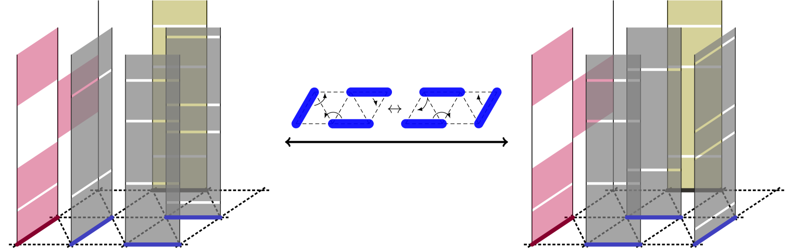
Figure 5: An example of a classical worm update for a three dimer resonance. The shaded regions correspond to dimer occupation at the corresponding imaginary time slice. The olive green membrane is a satisfying dimer but does not happen to be a part of the loop along which dimers are flipped, highlighting that not all satisfying dimers need to participate in an update. The red membranes do not satisfy the classical condition (due to a neighbor being occupied by a dimer for some region of imaginary time).

III.2 Quantum resonance update

Turning now to the quantum case, we begin by observing that the extended worm update discussed above will not be able to produce the types of configuration changes seen in Fig. 4. Thus these updates will completely miss the configurations which are a signature of the quantum spin liquid. We remedy this by proposing an update which specifically searches for possible pairs of resonances in the path integral configuration. Schematically, this proceeds by picking a random slice in imaginary time and first sweeping later positions in imaginary time to identify a possible location where a resonance is possible. Once this is found, we search in slices below the starting slice to see if we can find the same resonance. If so, we have identified a column which is bounded by a pair of identical resonances, and we can flip the dimers in the resonance to get a new configuration, as shown in Fig. 4. The mechanism of maintaining detailed balance during this process is quite involved and described in detail below. In the following, we refer to this update as the quantum resonance. We find that this update is essential in the correct sampling of path integral configurations in parameter regimes where the ground state resembles a $Z_{2}$ QSL. The resonances discussed above have already been used as an order parameter to detect a stable topological phase for a perturbed toric code Wu et al. (2012).

We explicitly sample the quantum resonances expected in the imaginary time direction using a construction of finite imaginary time tubes (with well defined ends) whose spatial cross-section resembles a dimer resonance on a closed loop. The update is carried out using a fixed loop size (smallest size being four, which corresponds to a nearest neighbor resonance as shown in Fig. 4) in the following manner :

1. We first calculate the maximal number of dimers on any single slice in the imaginary time direction in the current path integral configuration. Next, we identify all slices which have this maximal occupation, and pick one of these slices at random with uniform probability. For later reference, we label this slice at $s_{init}$. The column which we will flip will have end regions on either side of $s_{init}$.

2. We list all the dimers present in $s_{init}$ and store this as a reference spatial configuration. Now we sequentially travel up in the imaginary time direction and attempt to identify a suitable end region for our column. This is done at each subsequent slice by defining a “fuzzy” region of size $N/\Omega$, as this is the approximate size of imaginary time in which we can expect one dimer creation/annihilation event per lattice link.

3. For a resonance of size $l$, the number of dimers which must be created/annihilated in the fuzzy region must be $l/2$ (as shown for $l=4$ in Fig. 6). If this condition is satisfied in the fuzzy region, we check if the identified list of $l/2$ dimers (label this list as $d_{l/2}$) form a flippable loop. To simplify detailed balance, we consider the condition where only one such loop exists. This is technically challenging, and there are multiple ways to carry out this identification. We use a simple method of looping all possible neighboring links of $d_{l/2}$, and checking if this together with $d_{l/2}$ forms a valid loop. This process is exponential in $l$, but as resonances of size $l>6$ are extremely rare in the path integral as the highly correlated structure which generates them is highly improbable, we restrict ourselves to $l=4,6$. This avoids the exponential bottleneck and has no significant effect of efficiency of sampling.

4. Once a legitimate loop is identified, we fix the corresponding fuzzy region as the upper end of our update column. Now we must identify the same loop at some slice below $s_{init}$. We search sequentially the slices below $s_{init}$ until such a region is found using the same technical apparatus discussed above. A successful identification then defines the bottom end region.

5. We now flip the column along the loop, i.e. the dimers go from living on $d_{l/2}$ to its complement on the loop. In the operator string language of SSEQMC, this involves carrying all the operators living on the column to their new spatial positions as defined by the complement. This operation may create some inconsistencies with the path integral configuration which is not updated by this column flip. We check for such inconsistencies at this stage, and if identified we abort the update. For the type of resonances expected in a QSL, this is expected to happen rarely, and we see that our update still succeeds with an $O(1)$ probability.

6. To ensure that detailed balance is satisfied, we attempt to carry out the update in reverse by beginning at the same initial slice $s_{init}$. If the same $d_{l/2}$ and unique loop are found, then we carry out the flip along the loop in reverse. If at the end of this operation, the path integral configuration is exactly the same as the one before step 1 described above, then we have satisfied detailed balance, as probability $P(init\to final)=P(final\to init)$ and $P(init)=P(final)$. However, this is not always guaranteed and an example of the same is shown in Fig. 6. Applying the update on the final configuration (shown on the right) leads to an identification of a different column due to the arrangement of creation/annihilation events. Thus the update acting on the final configuration would not create the initial configuration (left one), and we reject this move as we cannot guarantee detailed balance.

The success of this update depends crucially on the presence of flippable columns. A reliable proxy for the same is the density of flippable plaquettes. We record this quantity in our simulations for the smallest $2\times 2$ plaquette and show our results in Fig. 8c for $\Omega=0.42$. In this regime, we expect a classical spin liquid at intermediate temperatures and indeed find that the density is lower than at low temperatures. At still lower temperatures, one can see that the density saturates as the ground state has been reached. Note that the temperature required for this saturation is much lower than all other scales in the problem, signifying that this is a low energy process. We find that the success probability for this update also saturates below a suitable temperature. Although all the results discussed here are for $L=4$, we expect the performance to be similar for larger system size, as the success depends only on column size, which is a finite number and is independent of $\beta$ (for large enough $\beta$) and system size $L$.

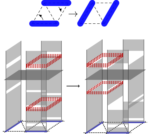
Figure 6: The quantum resonance update for the resonance shown (top). The update begins by using the reference state at a randomly chosen slice $s_{init}$ (shown as a horizontal plane here), and sweeping above and below this slice to identify fuzzy regions (marked by dashed red lines) where both the dimers are annihilated. These regions mark the ends of the update column, and we flip this column. The new configuration generated in the particular case shown does not generate the same modification on the backward move, as the left plaquette has become flippable now and is found before the right one (when searching below the $s_{init}$ plane). Thus this particular update does not obviously satisfy detailed balance and is rejected (discussed in detail in the sixth step of the quantum resonance update.)

III.3 Test of accuracy of updates

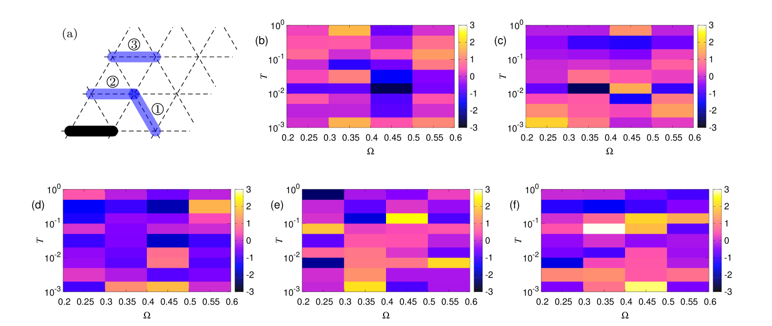
Figure 7: (a) Three correlation functions are calculated between the black bond, and the three numbered blue bonds. (d), (e) and (f) are the comparison with ED (using $R/\sigma^{N}$ as defined in text) for bonds number 1,2, and 3 respectively, with a relative error bar $\sigma^{N}$ of $O(10^{-2})$, (b) is for the energy with $O(10^{-4})$, and (c) for the dimer density with $O(10^{-3})$. In all cases, we see an agreement within $\pm 3$, in units of the error bars.

To get an intuition about the behavior of our system and to check the accuracy of our algorithm, we carry out a comparison with exact diagonalization for a small system size. The triangular lattice can in general be written as 3 lattice links (forming a triangle) sitting on each unit cell and the unit cells are arranged in a parallelogram with periodic boundary conditions. This is shown for $L=3$ in Fig. 2, and corresponds to a system with $3L^{2}$ links (Rydberg atoms). For odd $L$, it is not possible to have a fully packed dimer covering, as every dimer must have two unique end points. This implies that the $L=3$ lattice must host one empty lattice site, and the number of occupied links (excited Rydberg atoms) is at most four. The entire Rydberg allowed Hilbert space corresponds to all possible hard core dimer coverings (with any number of dimers). For $L=3$, the size of this space is $1126$, and this can be diagonalized fully without difficulty. This allows us to carry out a comparison with QMC at various values of temperature $T$ and $\Omega$.

To ensure that the QMC algorithm is sampling efficiently, we compare a few different quantities against exact diagonalization (ED). The comparison for an arbitrary observable $A$ is quantified by calculating the relative difference between the QMC and ED data, given by

$$R=(A_{QMC}-A_{ED})/A_{ED},$$ (4)

and normalizing $R$ by $\sigma_{QMC}$, which is the error from the QMC calculation. For all quantities we ensure that the normalized error $\sigma^{N}=\sigma_{QMC}/A_{QMC}$ is $O(10^{-2})$ or smaller. The exact values for different quantities are mentioned in the caption of Fig. 7. If the deviation from ED is within the QMC error bars, we would expect $R/\sigma^{N}$ to be $O(1)$, and this is the quantity plotted in Fig. 7. The most relevant observable to check is the energy, and this is usually the one with least noise in QMC. The comparison with ED is shown in Fig. 7, and we see that we can get at least a 4-digit match in this case. Due to the stability of energy in QMC, it is not always considered a good check of ergodicity, and as the updates we have proposed also improve sampling of spatial structure, we would like to compare average dimer density and various dimer-dimer correlations. The comparison for the dimer density $\braket{n}$ is shown in Fig. 7, and again we see a match which is of similar quality as the energy. We probe spatial structure by considering dimer correlation functions for three links with respect to a fixed link. These combinations are shown in Fig. 7. Note that due to the translation symmetry of the lattice, we can calculate the correlation function using all symmetry related pairs. However, here we want to study the accuracy with which the QMC estimates the correlation of a particular pair, and thus we do not use the symmetry related partners. Even after this, we find an agreement within $1\%$ of the ED values, for correlations which are themselves quite weak ($O(10^{-2})$). This is a rigorous check that the QMC is able to efficiently sample the spatial structure at all temperatures.

III.4 Advantage of using the quantum resonance update

To illustrate the utility of the quantum resonance, we study $L=4$ triangular lattices at low temperatures for a value of $\Omega$ (specifically $\Omega=0.42$) which we expect is in the correlated paramagnet regime. This expectation is justified by our study of the specific heat and string order parameters later in this manuscript, which shows a correlated paramagnetic behavior at $\Omega_{c}\lesssim 0.55$. features at small scales.

At high temperatures, the system samples all of Hilbert space uniformly, leading to a trivial paramagnet like phase. Upon lowering temperature, we find a two step lowering of the energy density, first to the CSL, and then to the correlated paramagnet (shown in inset of Fig. 8a). The zero is set here using the ground state energy from exact diagonalization, thus showing that the QMC approaches the correct value for $T\to 0$. The lower reduction of energy density is absent when we use only local updates and the classical worm update, implying that the sampling method is clearly insufficient.

Here we also show results for a more detailed study of the ergodicity by first analyzing the non-equilibrium behavior of our Monte Carlo simulation after equilibrating using just the classical worm update and local updates. We choose a temperature at which the ergodic simulations (with the quantum resonance update) confirm convergence to the ground state, and run our simulation without the quantum resonance update for $L=4$ in the correlated paramagnet regime ($\Omega=0.42$). Once equilibrium is reached using only the classical worm and local updates, the energy measured converges to $-0.1738(1)$, which is significantly higher than the true ground state energy $-0.174502003(1)$ from Lanczos diagonalization. We call this as the zero of our Monte Carlo time ($t_{MC}=0$), and now include the quantum resonance update in our simulation. As shown in Fig. 8b, the energy reduces to the required value in a fairly small number of Monte Carlo steps, thus showing that the quantum resonance update is able to access the true quantum ground state regime starting from the non-equilibrium configuration generated by using only the other updates.

To study the reason for the success of the quantum resonance update, one can calculate the average number of resonances on flippable plaquettes present in the path integral. Note that here the exact density can be considered only qualitatively, as we have calculated only the density of certain known and simple motifs strictly consecutive in the path integral, i.e. when the four operators required for a plaquette resonance follow each other in imaginary time. Although this is not likely to be true for most resonances (as intermediate operators which lie on other lattice sites are possibly present), this estimate is sufficient to give us a sense of the behavior with reducing temperature. We show our results in Fig 8c, and see that the density of resonances (per unit space-time, i.e. normalized by $N\beta$) grows with reducing temperature and saturates at the smallest temperatures (as expected when we reach the ground state).

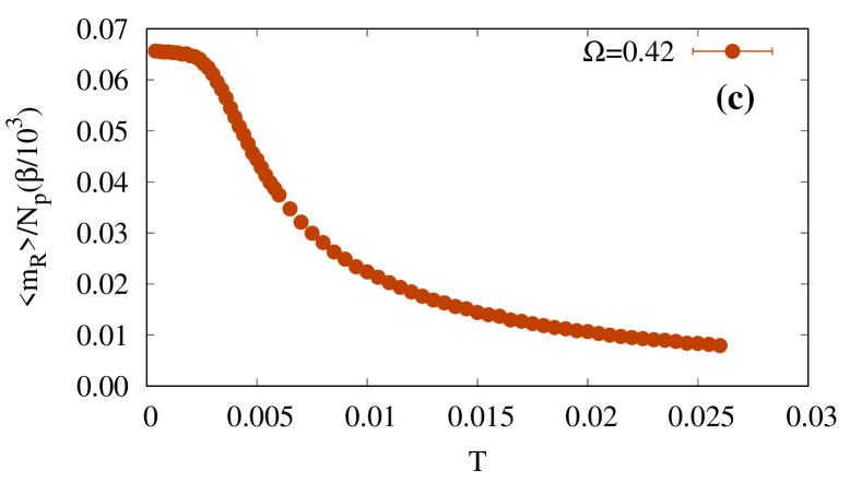
Figure 8: For $L=4$ at $\Omega=0.42$ : (a) Energy per link as a function of temperature for different updates. We shift the energy axis using our the ground state energy from Lanczos diagonalization, i.e. new ground state energy is zero. Without the quantum resonance algorithm, the simulation is unable to sample the low $T$ regime, inset zooms in on this using a linear scale for the energy. (b) Reduction of energy as a function of Monte Carlo time once the quantum resonance update is turned on at $T=0.001$. (c) Average number of resonances in the path integral, normalized by the number of possible $2\times 2$ resonating plaquettes and the average size of imaginary time required to converge to the ground state ($10^{3}$).

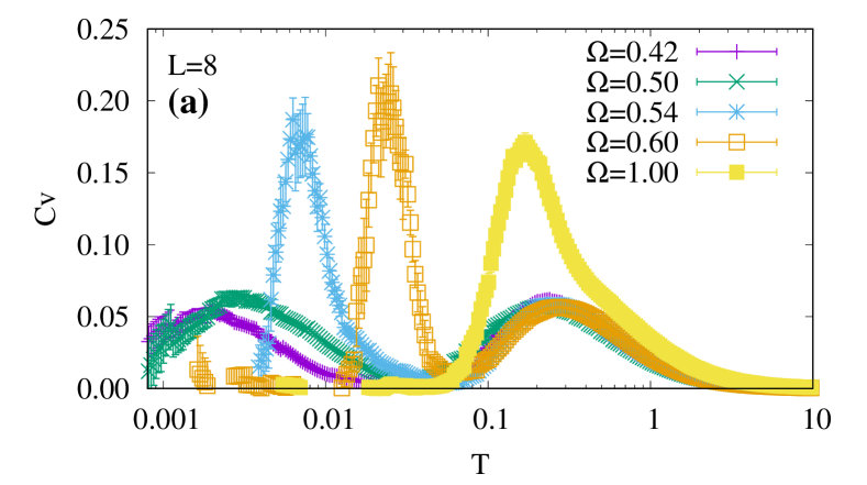
Figure 9: (a) Specific heat $C_{v}$ as a function of temperature $T$ for various values of $\Omega$ for $L=8$. (b) $C_{v}$ at fixed $\Omega=0.50$ for a range of sizes shows only weak finite size corrections. (c) Structure factor for $L=16$ at $T=0.0032$ and $\Omega=0.56$

IV Results for Triangular lattice

Let us first discuss the possible phases realized on the triangular lattice at low temperature. For $\Omega\gg\delta$, we expect a simple paramagnet, with low dimer density, and insignificant correlations between dimers. For $\Omega=0$, we should expect a classical spin liquid, i.e. degenerate ground states corresponding to fully packed dimer coverings. For $0<\Omega<\delta$, we can expect either a spin liquid, or some ordering with a large unit cell. One of the most robust metrics to develop a phase diagram is the specific heat, which we calculate from our Monte Carlo simulations by taking the numerical derivative of the energy with respect to temperature. As the temperatures we study are orders of magnitude smaller than the dominant scale $\delta$, we find that this method has substantially smaller error bars than those generated by using the fluctuation-dissipation theoremSandvik (2010).

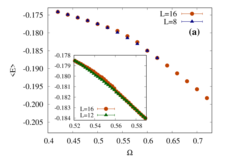
Figure 10: Energy (a) and monomer density (b) for a range of $\Omega$ at $T=0.0016$ and using $L=8$ and $16$ shows no sharp features, i.e. no quantum phase transition. Zoomed in versions for $L=12$ and $16$ also shown for $T=0.0032$.

Our results are shown in Fig. 9a, and we find that at $\Omega\approx\delta$, the specific heat shows a single peak. In this regime we expect a quantum paramagnet for the ground state and the specific heat peak is expected to be a smooth crossover from the thermal paramagnet. Upon lowering $\Omega$, we find a double peak structure, which signifies first the crossover to the classical spin liquid regime when approaching from high temperature, and then a crossover or transition to a unique ground state at low temperature. This is consistent with the picture at $\Omega=0$, where we expect only a single crossover from the high temperature paramagnet to the classical spin liquid. Note that at $\Omega=0$, we expect fully packed dimer coverings at zero temperature, as $\delta$ acts as a chemical potential for the dimers. However, for $\Omega\neq 0$, this is not the case, as the $\Omega$ term acts as a creation(annihilation) operator and the system can lower its energy by having a fluctuating number of dimers. Thus, in general, for all parameter regimes with $\Omega>0$, we expect a non-zero density of monomers. To check that we are indeed reaching the ground state for the parameter range for interest, we integrate the specific heat to get the entropy as a function of temperature. This analysis is shown in App. A, and we conclude that we are reaching the zero entropy regime for the lowest temperatures that we are able to access.

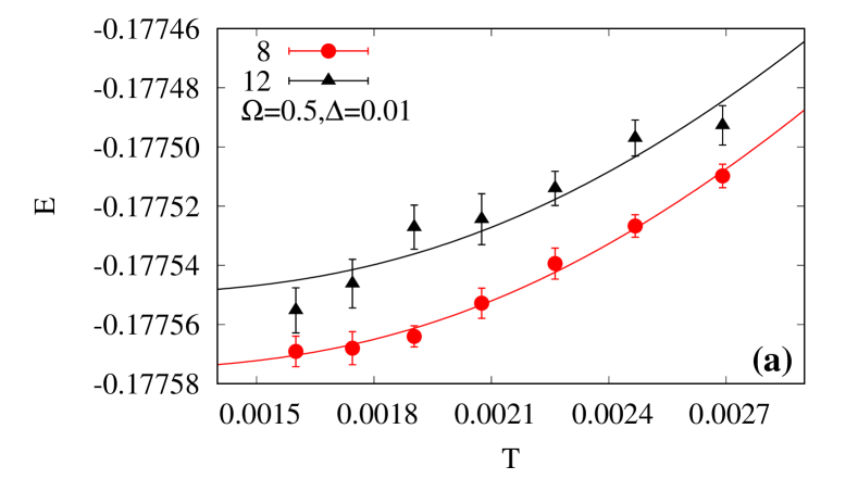
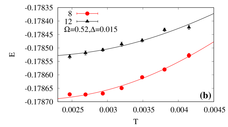
Figure 11: Energy as a function of temperature for $\Omega=(a)0.5,(b)0.52$ and $(c)0.54$. Fits to $a+be^{-\Delta/T}$ with the same $\Delta$ for system size $L=8$ and $12$. The fitted value of $\Delta$ is noted in the legend of each plot.

Figure 12: (a) Contour for $O^{z}_{FM}$. (b) Vanishing behavior for $L=12,T=0.0128$ as we move away from strongly paramagnetic regime. (c) Behavior consistent with $O^{x}_{FM}$ for $L=4$ exact diagonalization for ground state on loop configurations $a$-$d$ described in App. B.

IV.1 Investigation of quantum phase transition

The monomer density ($1/6-$dimer density) and energy as a function of $\Omega$ are shown in Fig. 10. There is a rapid change in the behavior of both quantities close to $\Omega=0.56$, which may lead one to suspect a quantum phase transition (QPT) from $Z_{2}$ QSL to trivial paramagnet around this value of $\Omega$. However, as we discuss below, analysis of the system size dependence and thermodynamic properties of our simulations does not support this conclusion. Instead, the simulations seem to show a smooth crossover in this regime, leading us to the conclusion that the putative QSL phase is not truly distinct from the trivial quantum paramagnet.

The inflection points in the energy and monomer density in Fig. 10 do not get significantly sharper on increasing system size from $L=8$ to $L=16$, which indicates against a QPT.

The absence of a quantum phase transition is further indicated from our $C_{v}$ data (Fig. 9a), which shows the gap (the lower temperature peak can be considered to be a proxy for this) is smoothly reducing with $\Omega$, rather than closing and opening again as we would expect for a transition between two gapped phases.

In the inset of Fig. 9b, we have plotted the low temperature behavior of the energy per link, and fit to the form $a+be^{-\Delta/T}$, with the same value for the gap $\Delta$ for system size $L=8$ and $12$. We find a good fit for $\Delta=0.03$ for $\Omega=0.56$. We also check the range of $\Omega\in(0.5,0.54)$ and find a finite gap for this region which is reducing with $\Omega$ as expected. These fits are shown in Fig. 11 and leads us to conclude that there is no closing of the gap at least down to $\Omega=0.5$.

To confirm that this is indeed a gapped point and not a QPT, we study $C_{v}$ for $L\in\{8,16\}$ and find no significant finite size effects, and an exponential decay of energy as $T\to 0$ (Fig. 9b). This signifies a finite energy gap at $\Omega=0.56$. The $C_{v}$ data shown in Fig. 9b clearly indicates that the two peaks seen in the temperature scans are crossovers and do not sharpen into phase transitions with increasing size. This confirms our expectation that the ground state is paramagnetic, and as a secondary check we can study the structure factor. Connecting the link centers of the triangular lattice leads to a Kagomé lattice, and thus we can use the definition of the structure factor for a spin system living on the same. Following Ref. Sherman and Singh (2018), we define the structure factor as

$$S(\vec{q})=\sum_{ab}\sum_{i_{1},i_{2}}\langle n_{a}(0,0)n_{b}(i_{1},i_{2})\rangle e^{-i\vec{q}\cdot(i_{1}\vec{R}_{1}+i_{2}\vec{R}_{2}+\vec{l}_{b}-\vec{l}_{a})},$$ (5)

where $(i_{1},i_{2})$ indexes a unit cell of the Kagomé lattice, $(a,b)$ index the site numbers within that unit cell and the lattice vectors defined as $\vec{R_{1}}=(2,0)\ ,\ \vec{R_{2}}=(1,\sqrt{3})\ ,\ \vec{l_{0}}=(0,0)\ ,\ \vec{l_{1}}=(-\frac{1}{2},\frac{\sqrt{3}}{2})\ ,\ \vec{l_{2}}=(\frac{1}{2},\frac{\sqrt{3}}{2})$ based on the geometry shown in Fig. 2. The correlation function $\langle n_{a}(0,0)n_{b}(i_{1},i_{2})\rangle$ used here is the connected version with $\langle n\rangle^{2}$ subtracted, where $\langle n\rangle$ is the mean dimer density. For $L=16,\Omega=0.5$ and $T=0.0032$, as shown in Fig. 9c, we find a featureless $S(\vec{q})$, supporting our previous conclusion that the ground state is either a paramagnet or a $Z_{2}$ QSL. In contrast to dimer models on bipartite lattices, it is known Fendley et al. (2002) that for the triangular lattice, even a fully packed classical dimer model has extremely short range correlations. This implies that no pinch point like structures are expected in $S(\vec{q})$.

It may be argued that since our simulations are conducted at finite temperature, a smooth crossover from a $Z_{2}$ QSL to a trivial paramagnet is expected in two dimensions, and that our results therefore do not contradict the existence of a $Z_{2}$ QSL at $T=0$. However, we note that our simulations reach the zero entropy regime, and so we would expect to see signatures of any singular behavior at $T=0$ in our simulations. Moreover, even at finite temperature we would expect to see the effects of a gap closing in the thermodynamic properties in the vicinity of a QPT, which is not found in our simulations.

IV.2 String and Fredenhagen-Marcu order parameters

Dimer coverings with a small number of monomers can be expected to retain the essential physics of fully-packed coverings. The topological character of dimer coverings is typically identified using string order parameters. However, even an arbitrarily small monomer density leads to string order parameters vanishing in the thermodynamic limit. This has lead to the use of the Fredenhagen-Marcu order parameter (FMOP) Fredenhagen and Marcu (1983), which can robustly identify topological signatures in such regimes. This has recently been used to characterize a topological transition in the perturbed toric code Xu et al. , and to identify a possible $Z_{2}$ spin liquid in a Rydberg atom array on the ruby latticeVerresen et al. (2021). Following the latter study, we define

$$O^{\alpha}_{FM}(l)=\frac{\braket{\prod_{i\in o_{l}}\sigma^{\alpha}_{i}}}{|\braket{\prod_{i\in c_{l}}\sigma^{\alpha}_{i}}|^{\frac{1}{2}}}$$ (6)

where $o_{l}(c_{l})$ corresponds to a open(closed) contour of size $l\crossproduct l$ (shown in Fig. 12), and $\alpha=x,z$ correspond to off-diagonal and diagonal terms respectively. The numerator and denominator individually are the open and closed string order parameters respectively. In terms of the creation/annihilation and density operators discussed above, $\sigma^{x}_{i}=b^{\dagger}_{i}+b_{i}$ and $\sigma^{z}_{i}=2n_{i}-1$. For a superposition of fully packed dimer coverings, the string order parameter along a closed contour (denominator in Eq. (6)) is unity irrespective of its perimeter. However, a vanishing density of dynamical monomers lead to an exponential decay with perimeter for the same quantity. In this case, the FMOP is the ratio of two exponentially decaying quantities, and acts as a proxy for the weights of open-string quantum fluctuations (movement of a single monomer) and of closed-string quantum fluctuations (flip of dimers along a closed contour)Xu et al. .

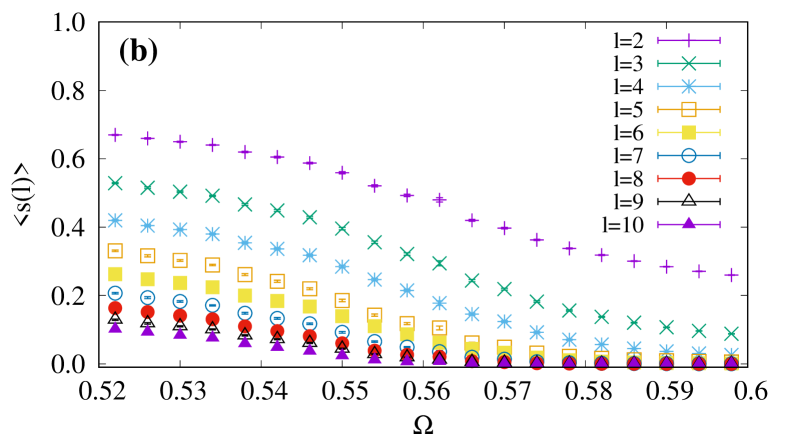
Figure 13: String order parameter defined over the contour shown in Fig. 12a with $l=2$ for a $4\times 4$ system. (a) $\braket{s(l)}$ for $L=16$ at $T=0.0016$ for various $l$ shows an increasing trend with reducing $\Omega$. Inset: Extrapolation of $\braket{s(l)}$ at $\Omega=0.42,0.54,0.56$ and $0.58$ as a function of $l$ (Faster decays with increasing $\Omega$). The last three data points (largest three values of $l$) are fit to $\braket{s(l)}=ae^{-l/b}$ to be consistent with $\lim_{l\to\infty}\braket{s(l)}\to 0$. (b) Same for $L=20$ close to $\Omega=0.56$ for $T=0.0045$, which is low enough to capture ground state physics for this range of $\Omega$ shows no sharp behavior.

For a $Z_{2}$ spin liquid, both $O_{FM}^{x}$ and $O_{FM}^{z}$ should vanish for large $l$Verresen et al. (2021). In contrast, for the paramagnetic regime, $\Omega\approx\delta$, the numerator and denominator of Eq. (6) both decay exponentially in a way which leaves the FMOPs finite. However, due to extremely small numerical values in the ratio, it is difficult to get small relative error bars for either $O_{FM}$ from Monte Carlo simulations. An added complexity for $O_{FM}^{x}$ is the fact that it is composed of strings of off-diagonal operators which suffer from extreme statistics in the SSEQMC formulationSandvik (2019). Thus we are only able to extract $O_{FM}^{z}$ up to $l=6$ with reasonable statistics from our simulations. To study $O_{FM}^{x}$, we resort to exact diagonalization for a $L=4$ system with various shapes for the contour. We fix temperature $T=0.0032$, which is expected to be low enough for the range of $\Omega$ we consider based on the $C_{v}$ data presented in Fig. 9, and present our results for the FMOPs in Fig. 12. We see that $O_{FM}^{z}$ reduces smoothly with decreasing $\Omega$, indicating that closed string dynamics are dominant over open string. This data is collected for $L=12$ at $T=0.0128$, which corresponds to the ground state for $\Omega>0.6$. The various loop geometries we have used for $O_{FM}^{x}$ are listed in App. B, and we see in Fig. 12c that all of them show a similar growth from zero close to $\Omega=0.5$. Thus we have signatures consistent with a $Z_{2}$ spin liquid for $\Omega\lesssim 0.5$.

We detect the same in the string order parameter as well, on a closed contour for $L=16$, as shown in Fig. 13 for various loop sizes $l$. Although its value is expected to vanish for $l\to\infty$ (inset of Fig. 13), we see a significant growth even for $l=8$ (which is the largest possible for $L=16$), with a change in behavior around $\Omega=0.56$.

Thus, although we have argued above on the basis of thermodynamic evidence that we do not see a QPT in this model, the FM order parameters do show signatures consistent with a $Z_{2}$ QSL for $\Omega\lesssim 0.56$. To resolve this, we propose that there is a regime for $\Omega\lesssim 0.56$ where the behavior of a $Z_{2}$ QSL is observable up to a finite length scale. This length scale is tunable with $\Omega$ and becomes smaller than a single lattice spacing for $\Omega>0.56$.

IV.3 Tunable scale for implementation of dimer constraint

Our results for the string order parameter on a closed loop suggest an exponential decay with loop size at a fixed $\Omega$. This is shown in the inset of Fig. 13a, and allows us to define a length scale over which we can expect the topological protection engineered by the fully packed dimer constraint. The closed string order parameter for the $l\times l$ loop can be considered to decay as $ce^{-l/\xi_{string}}$ and we can fit the numerical data to extract $\xi$ as a function of $\Omega$. The result of the fitting process is shown in Fig. 14 and we see that this scale smoothly decreases with increasing $\Omega$. The scale $\xi$ can thus be considered to be a proxy for the degree of topological protection, i.e. sizes $<\xi_{string}$ will behave as if they are perfectly topological and those with sizes $>\xi_{string}$ will behave like simple quantum paramagnets.

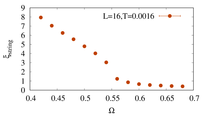
Figure 14: Length scale for topological protection $\xi_{string}$ as a function of $\Omega$ for $L=16,T=0.0016$, shows a smooth decay with increasing $\Omega$.

The PXP model we have studied results in a quantum dimer model (QDM) at fourth order in perturbation theory which has only a kinetic term, i.e. $V=0$ in the QDM language Moessner and Sondhi (2001). It is known that for the triangular lattice QDM, this parameter range hosts an ordered ($\sqrt{12}\times\sqrt{12}$) ground stateMoessner and Sondhi (2001). This supports our finding that there is no true $Z_{2}$ spin liquid for the small to intermediate values of $\Omega$ we have studied, although we do not see translational symmetry breaking in our simulations. For intermediate values of $\Omega$ we see a regime that seems smoothly connected to a quantum paramagnet, albeit with strong remnant similarities to a $Z_{2}$ spin liquid for intermediate scales. At finite temperature, the crossover from the CSL to the quantum paramagnet when increasing $\Omega$ can look like a phase transition due to a quick change in dimer density and the string order parameter. This is discussed in detail in App. C for $T=0.0128$ (which is much smaller than the microscopic energy scales), and implies that care must be taken when trying to identify a quantum phase transition from numerical simulations Yan et al. (2022).

V Conclusions

We have studied the PXP model in the reduced Hilbert space enforced by Rydberg blockade constraints on a triangular lattice. Our numerical simulations show the presence of a paramagnetic ground state for the relevant range of the strength of laser driving $\Omega$, with a tunable scale for topological protection built in and controlled by $\Omega$. We arrive at the conclusion about topological protection using an appropriately defined string order parameter, and studying its behavior with varying $\Omega$. A similar behavior of the string order parameters has been seen for the Kagomé latticeWang and Pollet (2024) where the QMC simulations have been unable to access the quantum spin liquid regime, but have found similar partial topological protection in the classical spin liquid regime. Our results suggest that topological protection up to a tunable length scale can be engineered in Rydberg atom arrays, and that this differs from the perfect topological protection seen in quantum dimer models as it hosts dimer coverings which are not fully packed. This may even be a possible interpretation for recent observations of topological protection in a triangular lattice quantum dimer model with monomers Yan et al. (2022), where topological features at finite scale (in particular the string order parameter for a small loop) have been interpreted as evidence for a $Z_{2}$ QSL. A recent study for a Rydberg atom array in 3D has also found similar results Wang et al. (2025), i.e. monomers may lead to a trivial state but for small system size spin liquid signatures (in their case a $U(1)$ Coulomb liquid is considered) can be retained.

To achieve the results we have presented in this paper, we have introduced a sampling of quantum resonances in the path integral representation. We have shown that without this sampling method, the crossover between the CSL and the quantum paramagnetic regimes of interest is impossible to capture, thus making it a necessary ingredient in our numerical recipe. This is especially important to Rydberg atom arrays, as this is a notoriously hard regime to sample using Monte Carlo simulations, with hurdles having been recently identified Yan et al. (2023); Hibat-Allah et al. (2024). As the resonances sampled are expected to be a general feature at least for $Z_{2}$ QSLs and similar phases Zhang and Cai (2024), our algorithm can readily be adapted to other model Hamiltonians which may host such states, such as quantum dimer models, XXZ models on the pyrochlore lattice, and frustrated transverse field Ising models.

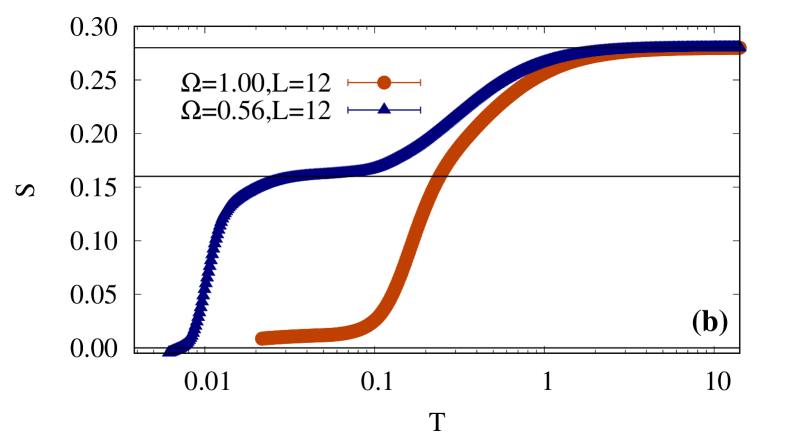
Figure 15: (a) Specific heat for $L=12$ as a function of temperature shows two well defined peaks. (b) Integration of $C_{v}/T$ for $\Omega=1$ and $0.56$ shows the residual entropy plateaus corresponding to the CSL and the full hard core dimer Hilbert space.

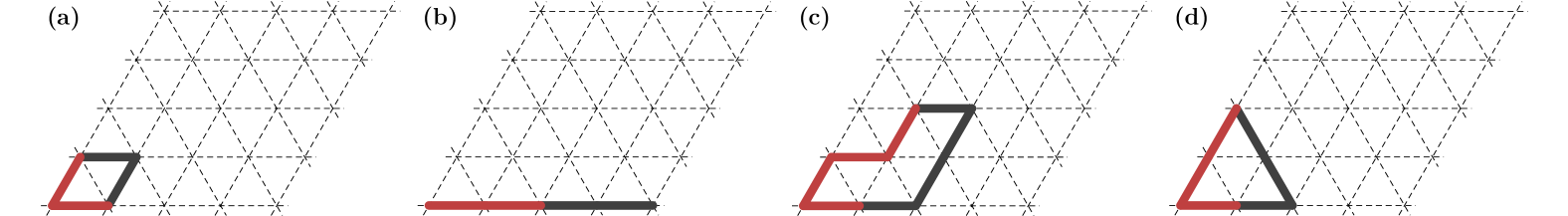
Figure 16: The various patterns of closed loops used to calculate $O^{x}_{FM}$ in Fig. 12. Red bonds corresponds to the portions used to calculate the open segments.

VI Acknowledgements

We would like to thank Zhenjiu Wang, Frank Pollmann, Claudio Castelnovo, Ciaran Hickey, Rhine Samajdar, Han Yan, Zheng Yan and Lode Pollet for useful discussions. Numerical simulations for this project were carried out using resources provided by the Max-Planck-Institut für Physik komplexer Systeme (MPIPKS) and Okinawa Institute of Science and Technology. We also acknowledge the support of the MPIPKS, where this project began.

Appendix A Specific heat and entropy for $L=12$

To illustrate the utility of the quantum resonance, we study $L=12$ triangular lattices at low temperatures for a value of $\Omega$ (specifically $\Omega=0.56$) which we expect is in the correlated paramagnet regime. As discussed in the main text, the specific heat should show two peaks as a function of temperature in this regime. This is shown clearly in Fig. 15 for $L=12$, where we have used both the classical worm and quantum resonance updates, and local updates developed in Ref. Patil (2023). As we calculate the specific heat by calculating the derivative of energy versus temperature, and cannot achieve small error bars for low temperatures due to the large computational resource requirement, $C_{v}$ at temperatures below $0.005$ have substantial error bars. However, at these temperatures the simulation is already sampling the ground state, and thus not relevant to our study.

The specific heat data for $L=12$ can be utilized to study the thermodynamic entropy as a function of temperature. This is done by integrating $C_{v}/T$, and usually requires one to know the value of the entropy at one of the limits (either $T\to 0$ or $T\to\infty$). As the restricted Hilbert space in which our model operates has an unknown entropy at $T\to\infty$ (as the states are made of complex dimer coverings), we must use the opposite limit, i.e. $T\to 0$. This limit can be utilized in the paramagnetic regime ($\Omega\approx 1$), where we know that the ground state should have zero residual entropy. We use the integral at $\Omega=1$ to get the entropy of the restricted Hilbert space as $T\to\infty$, and find this to be $0.28(1)$ per link, which is significantly smaller than $ln(2)\approx 0.693$, which would be the case for uncorrelated links. The entropy as $T\to\infty$ should be the same for all values of $\Omega$, and thus we use this value as the upper limit when performing the integration in the correlated paramagnet regime at $\Omega=0.56$. We find that there is a plateau at intermediate temperatures which is associated with the CSL, with a residual entropy per link of $0.16(1)$, and an eventual drop to zero entropy within the error bars from our specific heat data. This is shown for our $L=12$ $C_{v}$ data in Fig. 15, and leads to the conclusion that in the correlated paramagnet regime we are able to reach temperatures where we have converged to the ground state.

Appendix B Loop arrangements for calculating $O^{x}_{FM}(l)$ from exact diagonalization

As mentioned in Sec. IV, the off-diagonal FM order parameter $O^{x}_{FM}(l)$ cannot be calculated to high accuracy using QMC due to large fluctuations in the estimators. Thus the data presented for the same in Fig. 12c is for an $L=4$ lattice using exact diagonalization. As this prevents us from performing any scaling with loop size, we instead show in Fig. 12c that the behavior of $O^{x}_{FM}$ is robust for different loop shapes. The loop configurations for which we have calculated this data (denoted by type $a$-$d$ in Fig. 12c) are shown in Fig. 16. Each loop is of even length, and the open string is highlighted in red, whereas its partner which completes the closed loop is shown in black.

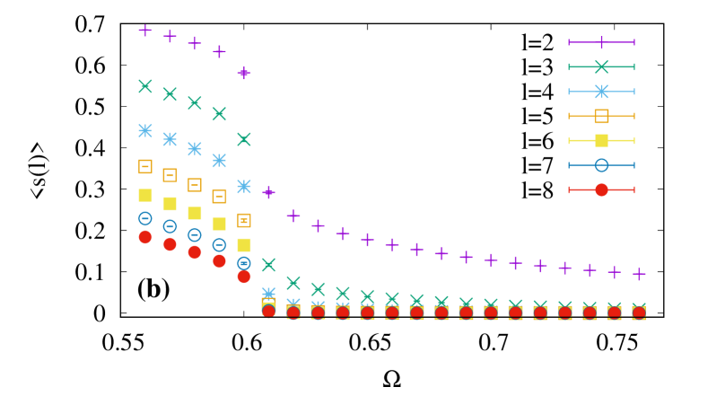
Figure 17: (a) Monomer density and (b) string order parameter for closed strings for a range of $l$ as a function of $\Omega$ for $T=0.0128$ and $L=16$.

The single plaquette resonance loop in Fig. 16a can be taken to be a direct estimate of the smallest quantum resonance possible on the triangular lattice. Fig. 16b represents a loop which winds around the system, and is thus topologically non-trivial. However, as seen in Fig. 12c, this does not affect the behavior as we are not considering a fully packed dimer model. Fig. 16c represents the longest loop which we have tested, and is made up of eight links and does not enclose any sites of the triangular lattice. Fig. 16d is the only loop which we have considered where the open string has an odd number of links. However, we find that this does not significantly affect its behavior as a function of $\Omega$.

Appendix C Crossover between classical spin liquid and quantum paramagnet

Here we discuss the crossover between the classical spin liquid regime and the quantum paramagnet when tuning $\Omega$ at finite $T$. We choose $T=0.0128$ as we have seen in Fig. 9 that this temperature is higher than the location of the low temperature peak. This implies that there is still some residual entropy at this temperature for $\Omega=0.56$, which is close to where we see the crossover. As shown in Fig. 17, we see that the monomer density and the string order parameter (as defined in Sec. IV) rapidly change near the crossover. The CSL regime is characterized by the monomer density vanishing, and the string order parameter being sizable for small $l$. Note that as the monomer density is non-zero in the range of $\Omega$ which we have studied. This implies that for $l\to\infty$, the string order parameter should vanish, and this is consistent with the data presented in Fig. 17.

References

- Jaksch et al. (2000) Dieter Jaksch, Juan Ignacio Cirac, Peter Zoller, Steve L Rolston, Robin Côté, and Mikhail D Lukin, “Fast quantum gates for neutral atoms,” Physical Review Letters 85, 2208 (2000).
- Lukin et al. (2001) Mikhail D Lukin, Michael Fleischhauer, Robin Côté, LuMing Duan, Dieter Jaksch, J Ignacio Cirac, and Peter Zoller, “Dipole blockade and quantum information processing in mesoscopic atomic ensembles,” Physical review letters 87, 037901 (2001).
- Urban et al. (2009) E Urban, Todd A Johnson, T Henage, L Isenhower, DD Yavuz, TG Walker, and M Saffman, “Observation of rydberg blockade between two atoms,” Nature Physics 5, 110–114 (2009).
- Browaeys and Lahaye (2020) Antoine Browaeys and Thierry Lahaye, “Many-body physics with individually controlled rydberg atoms,” Nature Physics 16, 132–142 (2020).
- Bluvstein et al. (2021) Dolev Bluvstein, Ahmed Omran, Harry Levine, Alexander Keesling, Giulia Semeghini, Sepehr Ebadi, Tout T Wang, Alexios A Michailidis, Nishad Maskara, Wen Wei Ho, et al., “Controlling quantum many-body dynamics in driven rydberg atom arrays,” Science 371, 1355–1359 (2021).
- Pan and Zhai (2022) Lei Pan and Hui Zhai, “Composite spin approach to the blockade effect in rydberg atom arrays,” Physical Review Research 4, L032037 (2022).
- Chen and Iadecola (2021) I-Chi Chen and Thomas Iadecola, “Emergent symmetries and slow quantum dynamics in a rydberg-atom chain with confinement,” Physical Review B 103, 214304 (2021).
- Verresen et al. (2021) Ruben Verresen, Mikhail D Lukin, and Ashvin Vishwanath, “Prediction of toric code topological order from rydberg blockade,” Physical Review X 11, 031005 (2021).
- Samajdar et al. (2021) Rhine Samajdar, Wen Wei Ho, Hannes Pichler, Mikhail D Lukin, and Subir Sachdev, “Quantum phases of rydberg atoms on a kagome lattice,” Proceedings of the National Academy of Sciences 118, e2015785118 (2021).
- Yan et al. (2022) Zheng Yan, Rhine Samajdar, Yan-Cheng Wang, Subir Sachdev, and Zi Yang Meng, “Triangular lattice quantum dimer model with variable dimer density,” Nature Communications 13, 5799 (2022).
- Semeghini et al. (2021) Giulia Semeghini, Harry Levine, Alexander Keesling, Sepehr Ebadi, Tout T Wang, Dolev Bluvstein, Ruben Verresen, Hannes Pichler, Marcin Kalinowski, Rhine Samajdar, et al., “Probing topological spin liquids on a programmable quantum simulator,” Science 374, 1242–1247 (2021).
- Zhou et al. (2017) Yi Zhou, Kazushi Kanoda, and Tai-Kai Ng, “Quantum spin liquid states,” Reviews of Modern Physics 89, 025003 (2017).
- Savary and Balents (2016) Lucile Savary and Leon Balents, “Quantum spin liquids: a review,” Reports on Progress in Physics 80, 016502 (2016).
- Kitaev (2003) A Yu Kitaev, “Fault-tolerant quantum computation by anyons,” Annals of physics 303, 2–30 (2003).
- Yan et al. (2019) Zheng Yan, Yongzheng Wu, Chenrong Liu, Olav F Syljuåsen, Jie Lou, and Yan Chen, “Sweeping cluster algorithm for quantum spin systems with strong geometric restrictions,” Physical Review B 99, 165135 (2019).
- Yan (2022) Zheng Yan, “Global scheme of sweeping cluster algorithm to sample among topological sectors,” Physical Review B 105, 184432 (2022).
- Merali et al. (2021) Ejaaz Merali, Isaac JS De Vlugt, and Roger G Melko, “Stochastic series expansion quantum monte carlo for rydberg arrays,” arXiv preprint arXiv:2107.00766 (2021).
- Yue et al. (2021) Mingxi Yue, Zijian Wang, Bhaskar Mukherjee, and Zi Cai, “Order by disorder in frustration-free systems: Quantum monte carlo study of a two-dimensional pxp model,” Physical Review B 103, L201113 (2021).
- Biswas et al. (2016) Sounak Biswas, Geet Rakala, and Kedar Damle, “Quantum cluster algorithm for frustrated ising models in a transverse field,” Physical Review B 93, 235103 (2016).
- Hearth et al. (2022) Sumner N Hearth, Siddhardh C Morampudi, and Chris R Laumann, “Quantum orders in the frustrated ising model on the bathroom tile lattice,” Physical Review B 105, 195101 (2022).
- Wu et al. (2023) Kai-Hsin Wu, Alexey Khudorozhkov, Guilherme Delfino, Dmitry Green, and Claudio Chamon, “ symmetry-enriched toric code,” arXiv preprint arXiv:2302.03707 (2023).
- Wu et al. (2021) Kai-Hsin Wu, Zhi-Cheng Yang, Dmitry Green, Anders W Sandvik, and Claudio Chamon, “Z 2 topological order and first-order quantum phase transitions in systems with combinatorial gauge symmetry,” Physical Review B 104, 085145 (2021).
- Moessner and Sondhi (2001) Roderich Moessner and Shivaji L Sondhi, “Resonating valence bond phase in the triangular lattice quantum dimer model,” Physical Review Letters 86, 1881 (2001).
- Fredenhagen and Marcu (1983) Klaus Fredenhagen and Mihail Marcu, “Charged states in z_2 gauge theories,” (1983).
- (25) WT Xu, F Pollmann, and M Knap, “Critical behavior of fredenhagen-marcu string order parameters at topological phase transitions with emergent higher-form symmetries,” arXiv preprint arXiv:2402.00127 .
- Yan et al. (2023) Zheng Yan, Yan-Cheng Wang, Rhine Samajdar, Subir Sachdev, and Zi Yang Meng, “Emergent glassy behavior in a kagome rydberg atom array,” Physical Review Letters 130, 206501 (2023).
- Turner et al. (2018) CJ Turner, AA Michailidis, DA Abanin, Maksym Serbyn, and Z Papić, “Quantum scarred eigenstates in a rydberg atom chain: Entanglement, breakdown of thermalization, and stability to perturbations,” Physical Review B 98, 155134 (2018).
- Fendley et al. (2004) Paul Fendley, Krishnendu Sengupta, and Subir Sachdev, “Competing density-wave orders in a one-dimensional hard-boson model,” Physical Review B 69, 075106 (2004).
- Zeng et al. (2024) Zhongda Zeng, Giuliano Giudici, and Hannes Pichler, “Quantum dimer models with rydberg gadgets,” arXiv preprint arXiv:2402.10651 (2024).
- Sandvik (1992) Anders W Sandvik, “A generalization of handscomb’s quantum monte carlo scheme-application to the 1d hubbard model,” Journal of Physics A: Mathematical and General 25, 3667 (1992).
- Patil (2023) Pranay Patil, “Quantum monte carlo simulations in the restricted hilbert space of rydberg atom arrays,” arXiv preprint arXiv:2309.00482 (2023).
- Wang and Pollet (2024) Zhenjiu Wang and Lode Pollet, “The renormalized classical spin liquid on the ruby lattice,” arXiv preprint arXiv:2406.07110 (2024).
- Wu et al. (2012) Fengcheng Wu, Youjin Deng, and Nikolay Prokof’ev, “Phase diagram of the toric code model in a parallel magnetic field,” Physical Review B—Condensed Matter and Materials Physics 85, 195104 (2012).
- Sandvik (2010) Anders W Sandvik, “Computational studies of quantum spin systems,” in AIP Conference Proceedings, Vol. 1297 (American Institute of Physics, 2010) pp. 135–338.
- Sherman and Singh (2018) Nicholas E Sherman and Rajiv RP Singh, “Structure factors of the kagome-lattice heisenberg antiferromagnets at finite temperatures,” Physical Review B 97, 014423 (2018).
- Fendley et al. (2002) P Fendley, R Moessner, and Shivaji Lal Sondhi, “Classical dimers on the triangular lattice,” Physical Review B 66, 214513 (2002).
- Sandvik (2019) Anders W Sandvik, “Stochastic series expansion methods,” arXiv preprint arXiv:1909.10591 (2019).
- Wang et al. (2025) Jingya Wang, Changle Liu, Yan-Cheng Wang, and Zheng Yan, “Doped resonating valence bond states: How robust are the spin ice phases in 3d rydberg arrays,” arXiv preprint arXiv:2502.00836 (2025).
- Hibat-Allah et al. (2024) Mohamed Hibat-Allah, Ejaaz Merali, Giacomo Torlai, Roger G Melko, and Juan Carrasquilla, “Recurrent neural network wave functions for rydberg atom arrays on kagome lattice,” arXiv preprint arXiv:2405.20384 (2024).
- Zhang and Cai (2024) Tengzhou Zhang and Zi Cai, “Quantum slush state in rydberg atom arrays,” Physical Review Letters 132, 206503 (2024).