Bras and Kets in Euclidean Path Integrals

Abstract

Here we discuss the relation between bras and kets in Euclidean path integrals. In a theory lacking time-reversal or reflection symmetry, bras and kets differ by an operator ${\mathcal{T}}$ that complex conjugates the wavefunction and reverses the orientation of spacetime. In the presence of time-reversal and reflection symmetry, space is unoriented so ${\mathcal{T}}$ cannot be defined, but the time-reversal symmetry ${\sf T}$ is available instead. An important special case of this concerns the relation between the hermitian inner product ${\langle}~,~{\rangle}$ – linear in one variable, antilinear in the other – that is used to define quantum mechanical probabilities, and the symmetric bilinear operator $(~,~)$ that comes most naturally from the Euclidean path integral. They differ by the action of ${\mathcal{T}}$ or ${\sf T}$ on one side.

1 Introduction

In a scattering amplitude, initial states are mapped to final states. Somewhat similarly, an operator matrix element ${\langle}\Psi|{\rm O}|\chi{\rangle}$ has an initial state $\chi$ and a final state $\Psi$. The matrix element is linear in $\chi$ and antilinear in $\Psi$, because ${\langle}~|~{\rangle}$ is a hermitian form, not a bilinear one.

In this article, we will consider amplitudes coupling external states in Euclidean path integrals. We consider both closed and open universes, but conceptually the case of closed universes is particularly interesting. In fig. 1(a), we schematically depict a Euclidean path integral amplitude on a $D$-manfold $X$ with $n$ closed universe boundaries on which external states can be defined. Such amplitudes makes sense in any quantum field theory, but are of particular interest in topological field theories and also in the context of quantum gravity. An amplitude of this type, defined in the most natural way, is linear in each of the external states, and treats them symmetrically (so the amplitude is invariant under permutations of the external closed universes to the extent that such permutations extend to symmetries of the bulk manifold $X$; in gravity, such symmetry is achieved after summing over all choices of $X$). In such a picture there is no visible distinction between quantum mechanical bras and kets. In particular, if we set $n=2$ as in fig. 1(b), the Euclidean amplitude is bilinear in the two states, rather than being a hermitian pairing (linear in one state and antilinear in the other) like a quantum mechanical matrix element.

In the present article, we will analyze how to incorporate bras and kets in Euclidean path integrals. In particular, we will see what one should do in fig. 1(b) if one wishes to compute a hermitian pairing between the two states rather than a bilinear pairing.

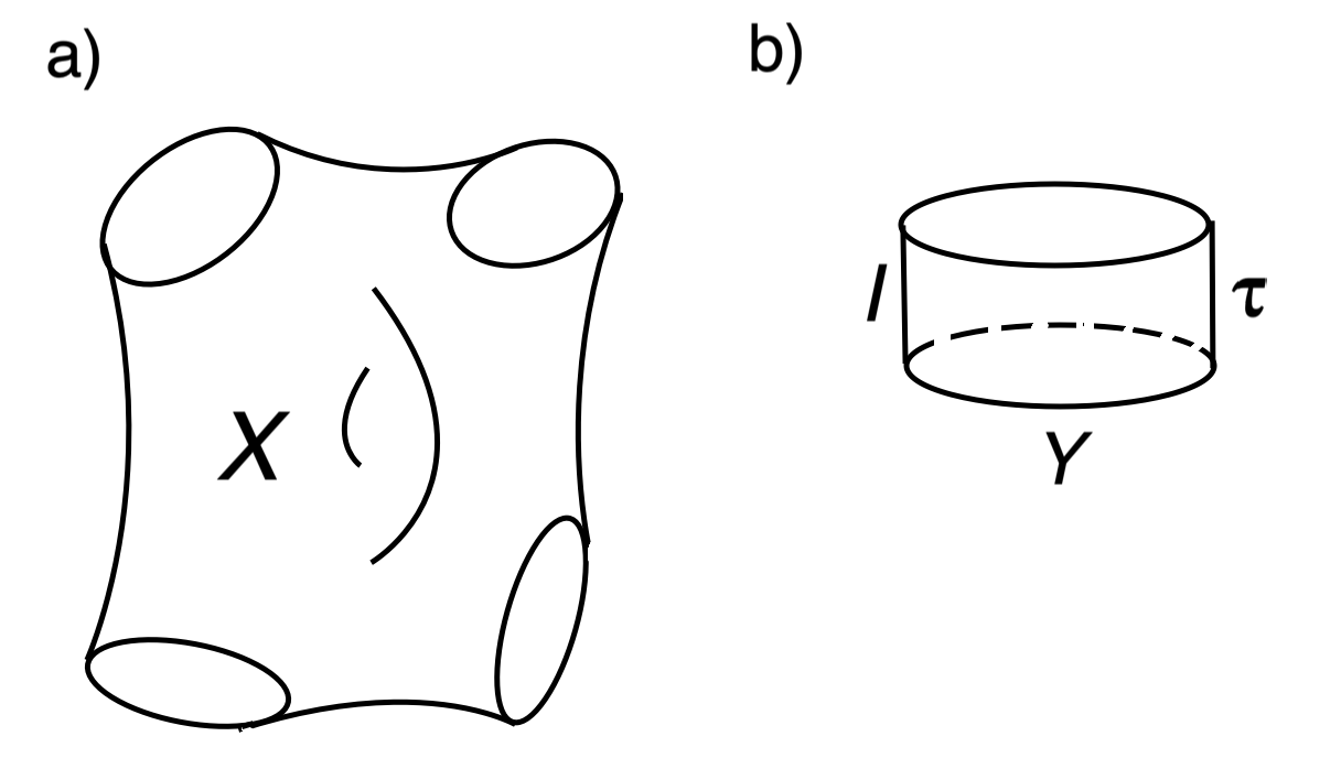
Figure 1: (a) A Euclidean $D$-manifold $X$ with $n$ boundary components, depicted here with $n=4$. The amplitude has bose/fermi symmetry in the external closed universe states. (b) The special case that $n=2$ and $X=Y\times I$, where $Y$ is a $D-1$-manifold and $I$ is an interval of width $\tau$. In quantum field theory without gravity, the bilinear pairing $(~,~)$ is defined by this path integral in the limit $\tau\to 0$. In topological field theory, there is no dependence on $\tau$. In a gravitational theory, one has to project such a path integral onto states that obey the gravitational constraints.

As one might expect, the answer involves the behavior of the quantum wavefunction under complex conjugation. In detail, there are two somewhat distinct cases depending on whether the theory is assumed to possess a symmetry of spatial reflection or time-reversal. The Standard Model of particle physics is an example of a theory with no such symmetry. In the absence of reflection symmetry, to define a quantum state on a spatial manifold $W$, in additional to specifying a functional of the fields on $W$, one has to pick an orientation of $W$. In a closed universe, this leads to a sort of doubling of the Hilbert space that is not usually taken into account (in an open universe, this doubling can be avoided by picking once and for all an orientation at spatial infinity). Roughly speaking, in the case of a theory with no time-reversal or reflection symmetry, a bra differs from a ket by complex conjugating the wave function and reversing the orientation of space. Theories with a reflection and time-reversal symmetry are more subtle. Roughly speaking, in such a theory there is no doubling associated with a choice of orientation – indeed, such theories can be formulated on unorientable manifolds – and a bra is obtained from a ket by acting with time-reversal.

In section 2, we discuss the relation between bras and kets in the relatively straightforward case of a theory that has no reflection symmetry. After presenting in section 3 some general background on reflection and time-reversal symmetries, we describe in section 4 the relation between bras and kets in theories with such symmetries. Actually, the discussion of time-reversal and reflection symmetries is more straightforward in the absence of fermions, so in section 4 we consider bosonic theories only. Fermions are included in section 5. The antilinear nature of ${\sf CPT}$ or ${\sf CRT}$ symmetry is discussed in an appendix.

${\sf CRT}$ symmetry in gravity has been recently discussed from another point of view in Harlow . A number of topics considered in the present article, such as reflection positivity in quantization on possibly unorientable manifolds, possibly with fermions, have been analyzed previously in detail in FH .

2 Theories With No Reflection Symmetry

2.1 An Example

A useful illustrative example of a quantum field theory with no reflection or time-reversal symmetry is a four-dimensional gauge theory with a theta-angle. The action in Lorentz signature is

$$I_{L}=-\frac{1}{4e^{2}}\int{\mathrm{d}}^{4}x\sqrt{g}\,{\mathrm{tr}}\,F_{\mu\nu}F^{\mu\nu}+\frac{\theta}{16\pi^{2}}\int{\mathrm{d}}^{4}x\sqrt{g}\epsilon^{\mu\nu\alpha\beta}{\mathrm{tr}}\,F_{\mu\nu}F_{\alpha\beta},$$ (1)

where $F$ is the gauge field and gauge field strength, $e$ and $\theta$ are the gauge coupling constant and theta-angle, $g$ is the spacetime metric tensor with signature $-+++$, $\epsilon_{\mu\nu\alpha\beta}$ is the Levi-Civita antisymmetric tensor, and (for the case of a gauge group ${\rm{SU}}(N)$ or ${\rm U}(N)$) ${\mathrm{tr}}$ is the trace in the fundamental representation. For an illustrative example of a theory of gravity with no reflection or time-reversal symmetry, we can simply take Einstein gravity coupled to a gauge theory with a theta-angle. A canonical example of a topological field theory with no reflection or time-reversal symmetry is three-dimensional Chern-Simons theory with a simple gauge group.

In Lorentz signature, the action of any unitary theory is always real; in particular, in (1) the parameters $e$ and $\theta$ are real. In Euclidean signature, the action of a theory that lacks reflection symmetry is not real. Indeed, when we transform from Lorentz to Euclidean signature, the metric tensor remains real, but the Levi-Civita tensor $\epsilon_{\mu\nu\alpha\beta}$ acquires a factor of ${\mathrm{i}}$. Thus the Euclidean action is

$$I_{E}=\frac{1}{4e^{2}}\int{\mathrm{d}}^{4}x\sqrt{g}{\mathrm{tr}}\,F_{\mu\nu}F^{\mu\nu}-\frac{{\mathrm{i}}\theta}{16\pi^{2}}\int{\mathrm{d}}^{4}x\epsilon^{\mu\nu\alpha\beta}{\mathrm{tr}}\,F_{\mu\nu}F_{\alpha\beta}.$$ (2)

We can make a simple general statement that would apply for any Lorentz-invariant action. The parity-violating terms are proportional to an odd power of $\epsilon_{\mu\nu\alpha\beta}$, so they are imaginary in Euclidean signature, while the parity-conserving terms are proportional to an even power of $\epsilon_{\mu\nu\alpha\beta}$, and are real. Accordingly under a reversal of orientation (which changes the sign of $\epsilon_{\mu\nu\alpha\beta}$), the Euclidean action is complex-conjugated. In a theory with fermions, the analysis is more complicated but the conclusion is the same: the Euclidean action in simple cases, and the effective action after integrating out fermions in general, is complex-conjugated under reversal of orientation. The fact that the path integral is complex-conjugated under reversal of orientation is essential in the proof of reflection positivity and thus unitarity; see fig. 2 for an explanation of this point. For a thorough analysis of reflection positivity in topological field theory (where arbitrary topologies have to be considered), in theories possibly with fermions and/or parity violation, see FH .

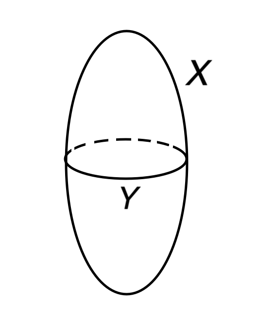
Figure 2: $X$ is a reflection-symmetric manifold that can be divided in two parts by cutting on its plane of symmetry $Y$. For any fixed values of the fields on $Y$, the path integral on the part of $X$ above the cut is the complex conjugate of the path integral on the part below the cut, because the reflection symmetry of $X$ reverses the orientation of $X$ and complex conjugates the action and the path integral. Hence for any values of the fields on $Y$, the product of the path integrals above and below $Y$ is positive. Upon integrating over fields on $Y$, this implies that the path integral on $X$ is positive. This property, known as reflection positivity, implies that the norm of the state on $Y$ that is prepared by the path integral on the lower portion of $X$ is positive. This is the basic argument proving positivity of Hilbert space norms in the context of path integrals.

A parity-violating theory cannot be defined on an unorientable manifold. It can only be defined on a manifold $X$ that is not just orientable but oriented, that is, a manifold on which an orientation has been chosen. We write $\varepsilon$ for the orientation of $X$. Concretely one can think of $\varepsilon$ as a choice of sign of the tensor $\epsilon_{\mu\nu\alpha\beta}$. Now write $Z_{X}(g,\varepsilon)$ for the partition function of a given theory on a manifold $X$ with a chosen metric $g$ and orientation $\varepsilon$. Denote the orientation opposite to $\varepsilon$ as $-\varepsilon$. Reversing the orientation complex conjugates the action, so it complex conjugates the argument $e^{-I_{E}}$ of the Euclidean path integral and therefore complex conjugates the partition function. Hence the partition function has a simple dependence on the orientation:

$$Z_{X}(g,\varepsilon)=\overline{Z_{X}}(g,-\varepsilon).$$ (3)

Of course, in a topological field theory (in which there is no dependence of physical observables on $g$) or a gravitational theory (in which we eliminate the dependence on $g$ by integrating over $g$), the partition function depends on $\varepsilon$ only, and not on $g$.

2.2 Orientations and Hilbert Spaces

Now we will study the physical states obtained in quantizing a $D$-dimensional theory that has no reflection symmetry on a spatial manifold $Y$ of dimension $D-1$. Naturally, in the absence of a reflection symmetry, the Hilbert space of physical states will depend on the orientation of $Y$. If $X$ is a Euclidean $D$-manifold with boundary $Y$, then a path integral on $X$, as a function of fields $\phi$ on $Y$, computes a physical state $\Psi(\phi)$. In Euclidean signature, a reversal of the orientation of $X$ will complex conjugate the action $I_{E}$ on $X$ and the path integral on $X$. So the state $\Psi(\phi)$ on $Y$ is also complex conjugated. This example indicates that there is a natural operation on physical states that reverses the orientation of $Y$ and complex conjugates the wavefunction.

It is instructive see this explicitly in the context of the gauge theory (1) with a theta-angle. To quantize the theory, we work on ${\mathbb{R}}\times Y$, with a Lorentz signature metric $-{\mathrm{d}}t^{2}+\sum_{i,j=1}^{3}h_{ij}{\mathrm{d}}x^{i}{\mathrm{d}}x^{j}$, where $t=x^{0}$ parametrizes ${\mathbb{R}}$, and $x^{i}$ are local coordinates on $Y$. Given a Levi-Civita tensor $\epsilon_{\mu\nu\alpha\beta}$ of $X={\mathbb{R}}\times Y$, we define a Levi-Civita tensor $\widetilde{\epsilon}_{ijk}=\epsilon_{0ijk}$ on $Y$.

Just as the path integral on $X$ depends on a choice of orientation of $X$, the Hamiltonian formalism on $Y$ depends on a choice of orientation of $Y$. To see this explicitly, we first compute the canonical momentum:

$$\Pi_{i}=\frac{1}{e^{2}}F_{0i}+\frac{\theta}{8\pi^{2}}\widetilde{\epsilon}_{ijk}F^{jk}$$ (4)

and the Hamiltonian

$$H =\int_{Y}{\mathrm{d}}^{3}x\sqrt{h}\,{\mathrm{tr}}\left(\frac{1}{2e^{2}}{\mathrm{tr}}\,F_{0i}(x)^{2}+\frac{1}{4e^{2}}{\mathrm{tr}}\,F_{ij}F^{ij}\right)$$ (5)

$$=\int_{Y}{\mathrm{d}}^{3}x\sqrt{h}\,{\mathrm{tr}}\left(\frac{e^{2}}{2}\left(\Pi_{i}(x)-\frac{\theta}{8\pi^{2}}\widetilde{\epsilon}_{ijk}F^{jk}(x)\right)^{2}+\frac{1}{4e^{2}}{\mathrm{tr}}\,F_{ij}F^{ij}\right).$$ (6)

In the gauge $A_{0}=0$, a physical state is a gauge-invariant function $\Psi(A_{i}(x))$. Upon canonical quantization, $\Pi_{i}(x)$ is replaced by $-{\mathrm{i}}\frac{\delta}{\delta A_{i}(x)}$, so the Hamiltonian acts by

$$H=\int_{Y}{\mathrm{d}}^{3}x\sqrt{h}\,{\mathrm{tr}}\left(\frac{e^{2}}{2}\left(-{\mathrm{i}}\frac{\delta}{\delta A_{i}(x)}-\frac{\theta}{8\pi^{2}}\widetilde{\epsilon}_{ijk}F^{jk}(x)\right)^{2}+\frac{1}{4e^{2}}{\mathrm{tr}}\,F_{ij}F^{ij}\right).$$ (7)

The Hamiltonian depends on the Levi-Civita tensor $\widetilde{\epsilon}$, or equivalently, it depends on the orientation $\varepsilon_{Y}$ of $Y$. Thus in quantizing the theory, we need to specify the orientation $\varepsilon_{Y}$ as well as the metric $g$ of $Y$. We will leave implicit the metric dependence (which is absent in a topological field theory, while in a theory of gravity the metric is one of the fields the wavefunction depends on) and denote the Hilbert space as ${\mathcal{H}}_{Y,\varepsilon_{Y}}$.

We see immediately that $H$ is hermitian but not real, and if we reverse the sign of $\widetilde{\epsilon}$, then $H$ is complex conjugated. The Hamiltonian operator acting on ${\mathcal{H}}_{Y,\varepsilon_{Y}}$ is thus the complex conjugate of the Hamiltonian operator acting on ${\mathcal{H}}_{Y,-\varepsilon_{Y}}$. Accordingly, there is a natural antilinear map ${\mathcal{T}}:{\mathcal{H}}_{Y,\varepsilon_{Y}}\to{\mathcal{H}}_{Y,-\varepsilon_{Y}}$ between the two Hilbert spaces by complex conjugation of the wavefunction:

$${\mathcal{T}}\Psi(A)=\overline{\Psi}(A).$$ (8)

This map conjugates the Hamiltonian acting on one Hilbert space to the Hamiltonian acting on the other. The operator ${\mathcal{T}}$ is antiunitary and satisfies

$${\mathcal{T}}^{2}=1.$$ (9)

We have used the example of gauge theory with a theta-angle to illustrate the fact that orientation reversal should be accompanied by complex conjugation of the wavefunction. However, the result is quite general. This is perhaps obvious in Euclidean signature: for $\beta>0$, since the action is complex-conjugated under reversal of orientation, the operator $e^{-\beta H}$, whose matrix elements are naturally computed by a Euclidean path integral, is complex-conjugated in a reversal of orientation, and therefore the same is true for $H$.

Since complex conjugating a hermitian operator such as the Hamiltonian is equivalent to taking its transpose, instead of saying that the Hamiltonian acting on ${\mathcal{H}}_{Y,\varepsilon_{Y}}$ is the complex conjugate of the Hamiltonian acting on ${\mathcal{H}}_{Y,-\varepsilon_{Y}}$, an equivalent statement is that these operators are transposes of each other. So if $H_{\varepsilon_{Y}}$ is the Hamiltonian acting on ${\mathcal{H}}_{\varepsilon_{Y}}$, and $H^{\rm tr}_{\varepsilon_{Y}}$ is its transpose, then

$$H^{\rm tr}_{\varepsilon_{Y}}=H_{-\varepsilon_{Y}}.$$ (10)

For applications to topological field theory or gravity, it is important that generically the orientable $D$-manifold $X$ or $D-1$-manifold $Y$ is not equivalent to the same manifold with the opposite orientation. Indeed, a generic orientable manifold (in dimension $\geq 3$) does not have any orientation-reversing diffeomorphism. For example, in four dimensions, a manifold such as ${\mathbb{CP}}^{2}$ with a nonzero signature has no orientation-reversing diffeomorphism; similarly, in three dimensions the Chern-Simons invariant of an abelian flat connection can be used to prove that a generic lens space $S^{3}/{\mathbb{Z}}_{n}$ does not have an orientation-reversing diffeomorphism. We will return momentarily to the case that $Y$ does have an orientation-reversing diffeomorphism.

The operation that we have called ${\mathcal{T}}$, being antilinear, is somewhat reminiscent of time-reversal symmetry, but it is not what is usually meant by time-reversal symmetry; indeed, we are discussing a theory with no time-reversal symmetry. In fact, ${\mathcal{T}}$ is not usually regarded as a symmetry. For example, the Standard Model is usually quantized in Minkowski space with a particular choice of spacetime orientation, defined perhaps by a “right hand rule.” Acting with ${\mathcal{T}}$ would exchange this quantization with an equivalent quantization of the Standard Model based on a left hand rule. This is not usually considered useful; it tells us nothing about what happens when the Standard Model is defined with the usual convention.

Matters are more subtle in the case of gravity. In that context, the two cases of an open universe and a closed universe are rather different. In semiclassical gravity, in an open universe, can pick an orientation once and for all at spatial infinity and that will always determine an orientation in the interior of the spacetime (or at least, the component of the spacetime that is connected to infinity). There is no need to consider any other orientation and so ${\mathcal{T}}$ plays no more role than it does for the Standard Model in Minkowski space.

More interesting is the case of a closed universe. In semiclassical quantization on closed universes, there is no natural way to avoid considering all orientable manifolds $Y$ with all possible orientations on $Y$. So, semiclassically, the Hilbert space is a direct sum

$${\mathcal{H}}=\bigoplus_{Y,\varepsilon_{Y}}{\mathcal{H}}_{Y,\varepsilon_{Y}}.$$ (11)

(For brevity, in writing this formula, we ignore the fact that some oriented $d$-manifolds $Y$ do have orientation-reversing diffeomorphisms; for such manifolds, we need not consider both choices of $\varepsilon_{Y}$.) We see that the Hilbert space ${\mathcal{H}}$ of closed universes has an antilinear symmetry ${\mathcal{T}}$ that exchanges ${\mathcal{H}}_{Y,\varepsilon_{Y}}$ with ${\mathcal{H}}_{Y,-\varepsilon_{Y}}$. Thus, ${\mathcal{H}}$ has a real structure; a state in ${\mathcal{H}}$ is “real” if the part of the wavefunction in ${\mathcal{H}}_{Y,\varepsilon_{Y}}$ is the complex conjugate of the part in ${\mathcal{H}}_{Y,-\varepsilon_{Y}}$. Should we treat ${\mathcal{T}}$ as a gauge symmetry, that is, are states that are invariant under ${\mathcal{T}}$ the only ones that we should consider to be physically sensible? It appears that the answer is “no” for the following reasons: (1) the gravitational path integral does not have a mechanism involving a sum over “twists” of some sort that would project onto ${\mathcal{T}}$-invariant states; (2) standard constructions via Euclidean path integrals construct states that are in general not ${\mathcal{T}}$-invariant (fig. 3) and there does not seem to be a good reason to reject such states. However, for possible arguments for a “yes” answer in holographic theories, see Harlow .

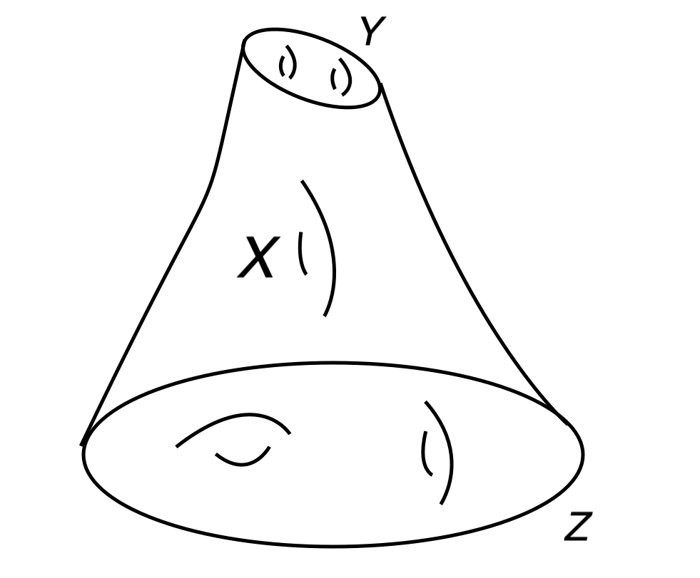
Figure 3: A state on a $D-1$-manifold $Y$ can be determined by asymptotic data at $Z$. A familiar version of this occurs with negative cosmological constant: $X$ can have Euclidean signature and $Z$ is the conformal boundary of $X$. With zero or positive cosmological constant, $X$ could be an expanding or contracting FRW spacetime in Lorentz signature with $Z$ at the far future or past. In all cases, with generic asymptotic data on $Z$, the induced state on $Y$ is not ${\mathcal{T}}$-invariant.

The four-dimensional gauge theory that we have considered as an example, even though it does not have a parity or time-reversal symmetry, does, if formulated in Minkowski space, have a combined symmetry usually called $\sf{CPT}$ (we will introduce an alternative terminology in section 3). In quantization on ${\mathbb{R}}^{3}$, $\sf{CPT}$ acts by parity, $(x^{1},x^{2},x^{3})\to(-x^{1},-x^{2},-x^{3})$ combined with the antiunitary operation of time-reversal. One may ask what is an analog of $\sf{CPT}$ for quantum field theory (or topological field theory, or quantum gravity) on a curved manifold $Y$. The closest analog arises if $Y$ does have an orientation-reversing symmetry ${\mathcal{R}}:Y\to Y$. Of course, ${\mathcal{R}}$ by itself is not a symmetry of a theory that lacks reflection symmetry, precisely because it reverses the orientation. But we can combine it with ${\mathcal{T}}$, which also reverses the orientation, to get an antilinear but orientation-preserving operation ${\mathcal{R}}{\mathcal{T}}$, which is a symmetry assuming the metric of $Y$ is ${\mathcal{R}}$-invariant. This operation, of course, is also a symmetry in a topological field theory or a theory of gravity.

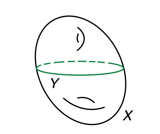
Figure 4: A path integral on a $D$-manifold $X$ can be “cut” on any embedded $D-1$-manifold $Y$. In a reflection-invariant theory of gravity, if $Y$ is compact and has an orientation-reversing symmetry $\rho$, one can glue the two sides of the cut back together after acting with $\rho$ on one side. A sum over such “twists” will project onto $\rho$-invariant states. Hence only $\rho$-invariant states can propagate. There is no close analog of this for ${\mathcal{T}}$ or for the time-reversal symmetries considered later.

For the same reasons as in the discussion of ${\mathcal{T}}$, it does not seem natural in the context of gravity to view ${\mathcal{R}}{\mathcal{T}}$ as a gauge symmetry. Indeed, the Euclidean path integral of fig. 3 can be used to prepare states that are not ${\mathcal{R}}{\mathcal{T}}$-invariant.

In general, if ${\mathcal{R}}$ and ${\mathcal{R}}^{\prime}$ are two different orientation-reversing symmetries of $Y$, then ${\mathcal{R}}{\mathcal{T}}$ and ${\mathcal{R}}^{\prime}{\mathcal{T}}$ are different as operators on ${\mathcal{H}}_{Y,\varepsilon}$. In topological field theory, ${\mathcal{R}}{\mathcal{T}}$ and ${\mathcal{R}}^{\prime}{\mathcal{T}}$ are equivalent if ${\mathcal{R}}$ and ${\mathcal{R}}^{\prime}$ are isotopic. In gravity in a closed universe, one expects that ${\mathcal{R}}{\mathcal{T}}$ does not depend on the specific choice of ${\mathcal{R}}$. The reason is that if ${\mathcal{R}}$ and ${\mathcal{R}}^{\prime}$ are orientation-reversing, then ${\mathcal{R}}^{\prime}{\mathcal{R}}^{-1}$ is orientation-preserving. In gravity in a closed universe, one would expect ${\mathcal{R}}^{\prime}{\mathcal{R}}^{-1}$ to behave as a gauge symmetry, leaving physical states invariant (see fig. 4). In that case ${\mathcal{R}}{\mathcal{T}}$ and ${\mathcal{R}}^{\prime}{\mathcal{T}}=({\mathcal{R}}^{\prime}{\mathcal{R}}^{-1}){\mathcal{R}}{\mathcal{T}}$ are equivalent.

For closed universes, ${\mathcal{T}}$ is the only universal antilinear symmetry that reverses the orientation of space (albeit in a trivial way, by exchanging any given spatial manifold $Y$ with another oppositely oriented copy of itself). So a case can be made for referring to ${\mathcal{T}}$ as ${\sf CRT}$ (the combination of time-reversal and a spatial reflection with charge conjugation; see section 3). We have not adopted this terminology here as ${\mathcal{T}}$ does not coincide with what would usually be called ${\sf CRT}$ in Minkowski space. It does seem, though, that any general hypothesis about a ${\sf CRT}$-like symmetry in the context of gravity should be formulated in terms of ${\mathcal{T}}$.

2.3 Bras and Kets and the Hermitian Inner Product

We are now prepared to answer the questions raised in the introduction. In a theory that lacks time-reversal or reflection symmetry, what is the relation between bras and kets in a Euclidean path integral such as that of fig. 1(a)? And in particular what is the relationship between the usual positive-definite hermitian inner product ${\langle}~,~{\rangle}$ on physical states, and the bilinear, permutation symmetric inner product $(~,~)$ that comes most naturally from the path integral of fig. 1(b)?

For this purpose, we first reconsider the claim that the general amplitude of fig. 1(a), involving a path integral on a bulk manifold $X$ with boundary components $Y_{r}$, $r=1,\cdots,n$ has permutation symmetry among the external states. The precise meaning of this statement depends on the type of theory considered. In a general quantum field theory, the amplitude is invariant under any permutations of the $Y_{r}$ that extend to orientation-preserving isometries of $X$. In topological field theory (where the metric of $X$ is irrelevant but the topology of $X$ is fixed), the amplitude is invariant under any permutations of the $Y_{r}$ that extend to orientation-preserving diffeomorphisms of $X$. Finally, in quantum gravity, the amplitude after summing over all choices of $X$ is potentially invariant under all permutations of the $Y_{r}$. Here, however, to explain the meaning of the statement, we have to be careful with orientations.

Let us consider carefully the amplitude of fig. 1(a), taking orientations into account. Once an orientation is picked on the bulk manifold $X$, it induces orientations on all of the boundary components $Y_{r}$. Concretely, along each $Y_{r}$, pick a Euclidean “time” coordinate $t_{r}$ that is constant along $Y_{r}$ and increases toward the interior of $X$, and pick local coordinates $x^{1},x^{2},\cdots x^{d}$ along $Y_{r}$. Then if $X$ has been oriented with a choice of Levi-Civita tensor that along $Y_{r}$ reduces to ${\mathrm{d}}t_{r}\,{\mathrm{d}}x^{1}\cdots{\mathrm{d}}x^{d}$, we orient $Y_{r}$ with the Levi-Civita form ${\mathrm{d}}x^{1}{\mathrm{d}}x^{2}\cdots{\mathrm{d}}x^{d}$. (Or we could reverse the sign and choose the orientation along $Y_{r}$ that corresponds to $-{\mathrm{d}}x^{1}{\mathrm{d}}x^{2}\cdots{\mathrm{d}}x^{d}$. The important thing is to use the same convention for all $X$ and for all components $Y_{r}$.)

For a general $X$, the induced orientations will not agree. Suppose that $n_{1}$ boundaries have one induced orientation and the other $n_{2}=n-n_{1}$ boundaries have the opposite induced orientation. This means that external states valued in ${\mathcal{H}}_{Y,\varepsilon}$ (for some $\varepsilon$) can be inserted on $n_{1}$ boundaries, and states valued in ${\mathcal{H}}_{Y,-\varepsilon}$ can be inserted on the other $n_{2}$ boundaries.

Beyond this point, what one would say depends on the application one has in mind. A point of view that is natural in gravity is to consider the amplitude of fig. 1(a) as a multilinear function on $n$ states valued in the direct sum ${\mathcal{H}}_{Y,\varepsilon}\oplus{\mathcal{H}}_{Y,-\varepsilon}$. This viewpoint is natural in the context of gravity, since ${\mathcal{H}}_{Y,\varepsilon}$ and ${\mathcal{H}}_{Y,-\varepsilon}$ both contribute to the closed universe Hilbert space (11). We simply then insert on each boundary the appropriate part of the state, whether valued in ${\mathcal{H}}_{Y,\varepsilon}$ or ${\mathcal{H}}_{Y,-\varepsilon}$, depending on the induced orientation of that boundary. After summing over all $X$ (and all orientations on each $X$), the amplitude understood this way has complete permutation symmetry in the external states.

Alternatively, what can we do if we want to consider all the external states to be valued in ${\mathcal{H}}_{Y,\varepsilon}$, with the same orientation? Such states can be inserted on the $n_{1}$ boundaries on which the induced orientation is $\varepsilon$. To insert ${\mathcal{H}}_{Y,\varepsilon}$-valued states on the $n_{2}$ boundaries with induced orientation $-\varepsilon$, we can first act with ${\mathcal{T}}$ to map these states to ${\mathcal{H}}_{Y,-\varepsilon}$, after which they can be inserted on the boundaries with that orientation. The result is to get an amplitude that is linear in $n_{1}$ copies of ${\mathcal{H}}_{Y,\varepsilon}$ and antilinear in $n_{2}$ additional copies of ${\mathcal{H}}_{Y,\varepsilon}$. In other words, this is an amplitude in which the external states consist of $n_{2}$ bras and $n_{1}$ kets. Amplitudes of this kind (usually with $n_{1}=n_{2}$) are often considered in calculations involving the replica trick (calculations that involve considering many copies of a quantum state).

If we assume that in gravity the state is supposed to be ${\mathcal{T}}$-invariant (contrary to what was argued previously in relation to fig. 3), then applying ${\mathcal{T}}$ to the part of the state valued in ${\mathcal{H}}_{Y,\varepsilon}$ just gives the part of the state valued in ${\mathcal{H}}_{Y,-\varepsilon}$. Once again, from this viewpoint, the sign of the induced orientation on the boundary distinguishes bras and kets.

A simple and important example is the special case $X=I\times Y$ of fig. 1(b), where $Y$ is a general orientable $d$-manifold and $I$ a closed interval that we parametrize by the Euclidean “time” $t$, with $0\leq t\leq\tau$. We will take the limit $\tau\to 0$ to define inner products, but it is clearest to start with $\tau>0$. In this example, no matter how we orient $X$, the induced orientations on the two boundaries are opposite. Let $x^{1},\cdots,x^{d}$ be local coordinates on $Y$, and suppose, for example, that $X$ is oriented by the Levi-Civita form ${\mathrm{d}}t\,{\mathrm{d}}x^{1}\cdots{\mathrm{d}}x^{d}$. Then $t$ increases in going away from one component but decreases away from the other, so the induced orientations on the two boundaries are opposite. Thus we can interpret this diagram as defining, in the limit $\tau\to 0$, a bilinear form $(~,~):{\mathcal{H}}_{Y,-\varepsilon}\otimes{\mathcal{H}}_{Y,\varepsilon}\to{\mathbb{C}}$. Alternatively, we can apply ${\mathcal{T}}$ to the first state and get a hermitian pairing ${\langle}~,~{\rangle}:{\mathcal{H}}_{Y,\varepsilon}\otimes{\mathcal{H}}_{Y,\varepsilon}\to{\mathbb{C}}$. Clearly the relation between the two pairings is

$${\langle}\Psi,\chi{\rangle}=({\mathcal{T}}\Psi,\chi).$$ (12)

Or we can apply ${\mathcal{T}}$ to the second state and get the complex conjugate hermitian pairing on the complex conjugate vector space ${\mathcal{H}}_{Y,-\varepsilon}$.

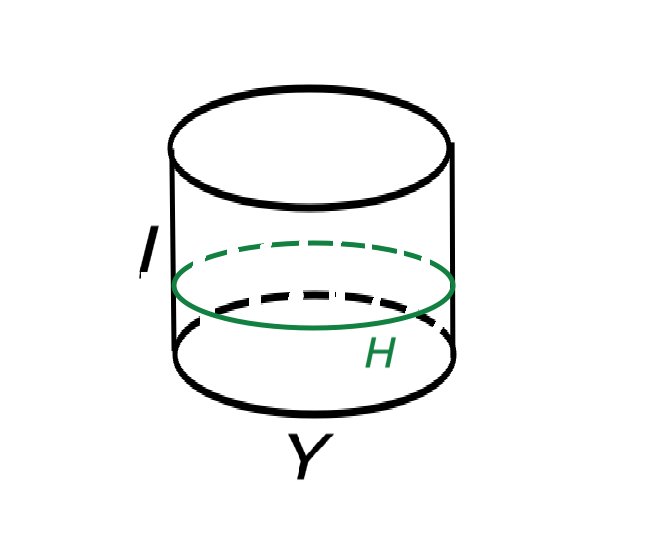
Figure 5: A path integral on $Y\times I$, where $I$ is an interval. The Hamiltonian $H$ has been inserted on the submanifold $Y\times p$, with $p$ a point in $I$. As $H$ is conserved, it can be freely moved to the top or bottom of the cylinder, implying that $(H\Psi,\chi)=(\Psi,H\chi)$. Thus $H$ is symmetric with respect to $(~,~)$, as well as hermitian with respect to ${\langle}~,~{\rangle}$. In a time-reversal invariant theory with time-reversal operator ${\sf T}$ that satisfies ${\sf T}^{2}=1$, a similar argument with ${\sf T}$ inserted on $Y\times p$, taking into account that ${\sf T}$ is antilinear, proves that $({\sf T}\Psi,\chi)=\overline{(\Psi,{\sf T}\chi)}$.

As a reality check, let us consider the example of the gauge theory with a theta-angle. In this example, $\Psi$ and $\chi$ are both functions of the gauge field $A$ on $Y$. The bilinear pairing $(\Psi,\chi)$ that comes from the $\tau\to 0$ limit of the cylinder amplitude of fig. 1(b) is formally an integral over the gauge field $A$ on $Y$:

$$(\Psi,\chi)=\frac{1}{{\rm vol}(\mathcal{G})}\int DA\,\Psi(A)\chi(A),$$ (13)

(here formally ${\rm vol}(\mathcal{G})$ is the volume of the group of gauge transformations on $Y$) and the corresponding hermitian pairing is

$${\langle}\Psi,\chi{\rangle}=\frac{1}{{\rm vol}(\mathcal{G})}\int DA\,\overline{\Psi}(A)\chi(A).$$ (14)

However, in (13), $\Psi(A)$ and $\chi(A)$ are vectors in Hilbert spaces ${\mathcal{H}}_{Y,-\varepsilon_{Y}}$ and ${\mathcal{H}}_{Y,\varepsilon_{Y}}$ defined with opposite orientations, while in (14), they take values in the same Hilbert space.

We can see the necessity of this distinction between the Hilbert spaces as follows. Let $H$ be the Hamiltonian operator of eqn. (7). Of course, it is supposed to be hermitian with respect to ${\langle}~,~{\rangle}$:

$${\langle}\Psi,H\chi{\rangle}={\langle}H\Psi,\chi{\rangle}.$$ (15)

There is no problem with this; the expression for $H$ in eqn. (7) is indeed manifestly hermitian. On the other hand, one can deduce from the path integral (fig. 5) that $H$ is also symmetric with respect to $(~,~)$:

$$(\Psi,H\chi)=(H\Psi,\chi).$$ (16)

However, it is not true that $H$ is equal to its own transpose, as this formula suggests. Rather, according to eqn. (10), taking the transpose of $H$ is equivalent to reversing the orientation of $Y$. In other words, eqn. (16) is valid if and only if $\Psi$ and $\chi$ are defined with opposite orientations on $Y$. Concretely, given this assumption, the proof of eqn. (16) is made by integrating by parts in the integral (13) that defines the bilinear pairing $(~,~)$. The two statements (15) and (16) are equivalent, given that $H$ commutes with ${\mathcal{T}}$.

In section 4, a different operator will play the role of ${\mathcal{T}}$ in relating the two inner products. So it will be useful to know, starting with a bose-symmetric bilinear pairing $(~,~)$, what properties the antilinear operator ${\mathcal{T}}$ must have so that eqn. (12) defines a hermitian pairing. A hermitian pairing is supposed to satisfy

$${\langle}\Psi,\chi{\rangle}=\overline{{\langle}\chi,\Psi{\rangle}}.$$ (17)

If ${\langle}~,~{\rangle}$ is defined as in eqn. (12), then this is equivalent to

$$({\mathcal{T}}\Psi,\chi)=\overline{({\mathcal{T}}\chi,\psi)}.$$ (18)

Because of the symmetry of $(~,~)$, the right hand side also equals $\overline{(\psi,{\mathcal{T}}\chi)}$, so ${\mathcal{T}}$ is the antilinear analog of a symmetric operator.

3 Background on Discrete Spacetime Symmetries

Before trying to generalize the preceding analysis to theories that do have reflection and time-reversal symmetries, we pause to discuss some general issues related to such symmetries. First of all, in four-dimensional Minkowski space, parity or ${\sf P}$ is usually defined to act, in some Lorentz frame, by a reflection of all three spatial coordinates, leaving the time fixed. Thus ${\sf P}$ maps $(t,x,y,z)$ to $(t,-x,-y,-z)$. On the other hand, time-reversal ${\sf T}$ is defined to map $t$ to $-t$ while leaving fixed the spatial coordinates. So the product ${\sf P}{\sf T}$ acts on spacetime by $(t,x,y,z)\to(-t,-x,-y,-z)$.

If a Lorentz-invariant theory is continued to Euclidean signature by setting $t=-{\mathrm{i}}t_{\sf E}$, then the resulting Euclidean theory automatically has a symmetry

$$(t_{\sf E},x,y,z)\to(-t_{\sf E},-x,-y,-z),$$ (19)

because this is simply the product of a $\pi$ rotation of the $t_{\sf E}-x$ plane with a $\pi$ rotation of the $y-z$ plane. The continuation of this symmetry back to Lorentz signature gives the universal symmetry that is usually called ${\sf CPT}$. Like other symmetries that reverse the sign of the time, ${\sf CPT}$ is represented by an antilinear rather than linear operator in quantum mechanics. It is not immediately apparent why this is the case; see Appendix A for an explanation. The reason that this symmetry is traditionally called ${\sf CPT}$, rather than ${\sf P}{\sf T}$, is that it anticommutes with all additive conserved or nearly conserved charges (such as baryon number, lepton number, and electric charge in the real world). To see why this is the case, observe that, as a rotation commutes with the symmetries generated by conserved charges, the Euclidean operation $(t_{\sf E},x,y,z)\to(-t_{\sf E},-x,-y,-z)$ commutes with those symmetries, and its continuation to Lorentz signature therefore also commutes with the symmetry group generated by the conserved charges. A typical element of that symmetry group is $e^{{\mathrm{i}}\alpha K}$, where $\alpha$ is a real parameter and $K$ is a real linear combination of hermitian conserved charges. As the symmetry that acts by $(t,x,y,z)\to(-t,-x,-y,-z)$ reverses the direction of time, it is antilinear and anticommutes with ${\mathrm{i}}$. To commute with $e^{{\mathrm{i}}\alpha K}$, it must then also anticommute with $K$, which is why it is traditionally called ${\sf CPT}$.

For a general value of the spacetime dimension $D$, the formulation in terms of ${\sf CPT}$ is inconvenient. Indeed, in $D$ dimensional Euclidean space, the operation

$$(t_{\sf E},x_{1},x_{2},\cdots,x_{D-1})\to(-t_{\sf E},-x_{1},-x_{2},\cdots,-x_{D-1})$$ (20)

is contained in the connected component of the rotation group, making it an automatic symmetry, if and only if $D$ is even. To define a ${\sf CPT}$-like symmetry in a way that is valid for any $D$, it is convenient to consider instead of ${\sf P}$ an operation ${\sf R}$ that reflects just one spatial coordinate. The operation $(t_{\sf E},x_{1},x_{2},\cdots,x_{d})\to(-t_{\sf E},-x_{1},x_{2},\cdots,x_{d})$ is a $\pi$ rotation of the $t_{\sf E}-x_{1}$ plane, so it is a symmetry in any rotation-invariant theory, regardless of $D$. This symmetry continues in Lorentz signature to a universal symmetry that we may call ${\sf CRT}$. Clearly, in contrast to ${\sf CPT}$, ${\sf CRT}$ can be defined for any value of $D$. In section 5, we explain a further simplification of ${\sf CRT}$ relative to ${\sf CPT}$.

In ordinary quantum field theory without gravity (and in topological field theory), one has a precise theorem stating that any Lorentz-invariant quantum field theory has the universal symmetry that we are calling ${\sf CRT}$. In gravity, there is no such precise theorem, but we do expect that a general gravitational theory does have ${\sf CRT}$ symmetry. This is true in semiclassical theories of gravity, it is true in perturbative string theory, it is true nonperturbatively in the AdS/CFT correspondence, and it is true in the framework of Euclidean path integrals considered in the present article.

${\sf CRT}$ is the only discrete spacetime symmetry that is universally expected in any theory, but many interesting theories have reflection and time-reversal symmetries as well. In the presence of such symmetries, there are several additional issues to consider. Before being general, let us recall that in the real world there are several additive conserved charges – notably electric charge, baryon number, and lepton number – that are exactly or at least very nearly conserved. The approximate discrete spacetime symmetries in the real world either commute or anticommute with these additive discrete charges. Therefore, the possible approximate time-reversal symmetries are ${\sf T}$ and ${\sf C}{\sf T}$, where ${\sf T}$ commutes with the conserved charges and ${\sf C}{\sf T}$ anticommutes with them, and similarly the possible approximate reflection symmetries are ${\sf R}$ and ${\sf C}{\sf R}$. These are the only approximate discrete spacetime symmetries in the real world, but in a general theory there are more possibilities. A time-reversal or reflection symmetry might commute with some conserved charges and anticommute with others, and it might not be possible to fully characterize a time-reversal or reflection symmetry by saying how it transforms the discrete charges; it may also be necessary to specify the action of the symmetry on fields of the theory. Thus the usual terminology used in particle physics is not adequate to discuss a general case.

Instead of complicating our notation to fully specify how a given reflection symmetry acts on conserved charges and other fields, we will simplify the notation and just write ${\sf R}$ for a reflection symmetry, and ${\sf T}$ for the corresponding time-reversal symmetry, defined so that the product ${\sf R}{\sf T}$ is the universal symmetry associated to a $\pi$ rotation in Euclidean signature. Thus, we will not specify in the notation how ${\sf R}$ or ${\sf T}$ acts on conserved charges or other fields and we will drop $\sf C$ from the notation.

If a given theory does have a reflection symmetry ${\sf R}$, it is not necessarily unique. If ${\sf R}$ is a reflection symmetry, and $\rm W$ is an “internal” symmetry, not acting on spacetime, then ${\sf R}^{\prime}={\sf R}{\rm W}$ is another reflection symmetry, albeit one that acts differently on the fields (and possibly on the conserved charges, if any are present). If we replace ${\sf R}$ with ${\sf R}^{\prime}$, we can compensate by replacing ${\sf T}$ with ${\sf T}^{\prime}={\rm W}^{-1}{\sf T}$. This will ensure that ${\sf R}^{\prime}{\sf T}^{\prime}={\sf R}{\sf T}$ is the universal symmetry associated to a $\pi$ rotation in Euclidean signature.

Reflection symmetries that satisfy ${\sf R}^{2}=1$ are of particular importance, for the following reason. Let us discuss the matter in Euclidean signature. First of all, any relativistic theory in Euclidean signature has at least ${\sf SO}(D)$ symmetry. If a theory also has a reflection symmetry that satisfies ${\sf R}^{2}=1$, then by adjoining this to ${\sf SO}(D)$ one gets an action of ${\sf O}(D)$ on the fields of that theory. The holonomy group of a possibly unorientable $D$-manifold $X$ is ${\sf O}(D)$ or a subgroup thereof. Thus an action of ${\sf O}(D)$ on the fields of a theory is what we need to define that theory on a general, possibly unorientable $D$-manifold $X$. In parallel transport around a closed loop $\gamma\subset X$, fields are transformed by the appropriate holonomy element in ${\sf O}(D)$, which will be an element of ${\sf SO}(D)$ or of the non-identity component of ${\sf O}(D)$ depending on whether the orientation of $X$ is preserved or reversed in going around $\gamma$.

If a reflection symmetry with ${\sf R}^{2}=1$ exists, it is not necessarily unique. To illustrate this point, consider a theory that has a reflection symmetry that satisfies ${\sf R}^{2}=1$, generating a group that we will call ${\mathbb{Z}}_{2}^{\sf R}$, and also an “internal” symmetry ${\mathbb{Z}}_{4}$, generated by an operator $\rm U$ that satisfies ${\rm U}^{4}=1$. In ordinary quantum field theory and in topological field theory, ${\mathbb{Z}}_{4}$ might be a global symmetry or a gauge symmetry; in gravity, we expect that ${\mathbb{Z}}_{4}$ will be a gauge symmetry BanksSeiberg ; HO ; emergence . In a theory with the combined ${\mathbb{Z}}_{2}^{\sf R}\times{\mathbb{Z}}_{4}$ symmetry, there are actually two reflection symmetries that square to 1, namely ${\sf R}$ and ${\sf R}{\rm U}^{2}$. The same theory also has reflection symmetries whose square is not 1, namely ${\sf R}\rm U$ and ${\sf R}{\rm U}^{3}$.

In a variant of this example, there is no reflection symmetry that satisfies ${\sf R}^{2}=1$. For this, it suffices to explicitly break the group ${\mathbb{Z}}_{2}^{\sf R}\times{\mathbb{Z}}_{4}$ to the group ${\mathbb{Z}}_{4}^{\prime}$ generated by ${\sf R}{\rm U}$. To do this, if ${\mathbb{Z}}_{4}$ is a global symmetry, we add to the action an operator that is invariant under ${\mathbb{Z}}_{4}^{\prime}$ but not under any other elements of ${\mathbb{Z}}_{2}^{\sf R}\times{\mathbb{Z}}_{4}$. This will give a theory that has the reflection symmetries ${\sf R}{\rm U}$ and $({\sf R}\rm U)^{3}={\sf R}{\rm U}^{3}$, but has no reflection symmetry whose square is 1. The ${\mathbb{Z}}_{4}^{\prime}$ symmetry can be gauged if we wish (assuming it is anomaly-free). A reflection symmetric theory that has no reflection symmetry whose square is 1 cannot be defined on a generic unorientable manifold. Such a theory can be defined on unorientable manifolds that possess a certain slightly exotic differential geometric structure.

In our further discussion of reflection-invariant theories, rather than exploring the more exotic possibilities mentioned in footnote 4, we assume that the reflection operator ${\sf R}$ can be chosen to satisfy ${\sf R}^{2}=1$. As we explained in the example of ${\mathbb{Z}}_{2}^{\sf R}\times{\mathbb{Z}}_{4}$, such a choice of ${\sf R}$ is in general not unique. Does the choice matter? If ${\sf R}$ and ${\sf R}^{\prime}$ are two reflection symmetries, then ${\rm W}={\sf R}{\sf R}^{\prime}$ is an “internal” symmetry (acting trivially on spacetime). If ${\rm W}$ is a global symmetry, then it does matter whether we use ${\sf R}$ or ${\sf R}^{\prime}$ to define the theory on an unorientable manifold. The different choices can give genuinely inequivalent ways to define the same theory on an unorientable manifold. If ${\rm W}$ is a gauge symmetry, the choice between ${\sf R}$ and ${\sf R}^{\prime}$ does not matter, since in any computation one will anyway be summing over all possible twists by ${\rm W}$, and the difference between using ${\sf R}$ or ${\sf R}^{\prime}$ to define the theory on an unorientable manifold is exactly such a twist. Of course, in gravity, one expects that ${\rm W}$ will always be a gauge symmetry, so that the choice of ${\sf R}$ will not matter. In what follows, we assume that, regardless of whether this choice is essentially unique or inequivalent choices would have been possible, we are given a specific reflection symmetry ${\sf R}$ whose square is 1.

Going back to Lorentz signature, we now want to discuss time-reversal. A choice of ${\sf R}$ determines a choice of ${\sf T}$, such that the product is the universal symmetry ${\sf R}{\sf T}$ related to a $\pi$ rotation in Euclidean signature. In the absence of fermions, ${\sf R}$ and ${\sf T}$ commute, because they arise in Euclidean signature from reflections in orthogonal directions (${\sf T}$ is a reflection of Euclidean time, and ${\sf R}$ is a reflection of a Euclidean space direction), which commute. Fermions will be included in section 5; for now, we assume that ${\sf R}$ and ${\sf T}$ commute. In the absence of fermions, $({\sf R}{\sf T})^{2}=1$, since in Euclidean signature ${\sf R}{\sf T}$ is just a $2\pi$ rotation. With ${\sf R}^{2}=({\sf R}{\sf T})^{2}=1$ and ${\sf T}$ commuting with ${\sf R}$, we have ${\sf T}^{2}=1$. This then defines the class of theories that we will consider in section 4: theories with chosen reflection and time-reversal symmetries ${\sf R}$ and ${\sf T}$ such that ${\sf R}{\sf T}$ is the universal symmetry related to a rotation in Euclidean signature and

$${\sf R}^{2}={\sf T}^{2}=1,~~{\sf R}{\sf T}={\sf T}{\sf R}.$$ (21)

In Minkowski space, ${\sf R}$ and ${\sf T}$ play somewhat similar roles as discrete spacetime symmetries, though they differ in that ${\sf R}$ is unitary and ${\sf T}$ is antiunitary. When we quantize a reflection-invariant theory on a general $D-1$-manifold $Y$ to get a Hilbert space ${\mathcal{H}}_{Y}$, ${\sf R}$ and ${\sf T}$ play very different roles. There is in general nothing that one could call reflection symmetry acting on ${\mathcal{H}}_{Y}$; such symmetries exist to the extent that $Y$ admits an orientation-reversing isometry. For general $Y$, there is no such isometry (and for some $Y$’s, there are many inequivalent ones so there are inequivalent ${\sf R}$-like symmetries). Rather, the role of ${\sf R}$ is that, as explained earlier, it enables us to define ${\mathcal{H}}_{Y}$ even if $Y$ is unorientable (and without choosing an orientation of $Y$ if $Y$ is orientable). By contrast, for any $Y$, ${\sf T}$ is an antilinear symmetry of ${\mathcal{H}}_{Y}$. This statement, however, is not quite trivial: it depends on the fact that ${\sf R}$ and ${\sf T}$ commute. If ${\sf T}$ and ${\sf R}$ did not commute, we would have ${\sf T}^{-1}{\sf R}{\sf T}={\sf R}^{\prime}$, where ${\sf R}^{\prime}$ is some other reflection symmetry. In that case, acting with ${\sf T}$ would map ${\mathcal{H}}_{Y}^{{\sf R}}$ to ${\mathcal{H}}_{Y}^{{\sf R}^{\prime}}$, where ${\mathcal{H}}_{Y}^{{\sf R}}$ and ${\mathcal{H}}_{Y}^{{\sf R}^{\prime}}$ are the Hilbert spaces of $Y$ defined using respectively ${\sf R}$ or ${\sf R}^{\prime}$. Something like this actually happens in the presence of fermions, as explained in section 5. But for now we assume that ${\sf R}$ and ${\sf T}$ commute, in which case ${\sf T}$ can always be defined as an antilinear symmetry of ${\mathcal{H}}_{Y}$. In a theory of gravity, for the same reasons as in the discussion of ${\mathcal{T}}$ in section 2.2, it seems that we should not consider ${\sf T}$-invariant states to be the only physically sensible ones.

Since ${\sf T}$ is a natural symmetry of any ${\mathcal{H}}_{Y}$ and ${\sf R}$ is not, it follows that also there is no natural ${\sf R}{\sf T}$ symmetry of ${\mathcal{H}}_{Y}$. Any such symmetry depends on the existence and choice of an orientation-reversing symmetry of $Y$. In the case of gravity in a closed universe, if $Y$ does have an orientation-reversing symmetry $\rho$, then $\rho$ will behave as a gauge symmetry (fig. 4).

4 Theories With A Reflection Symmetry

We now consider a theory with chosen ${\sf R}$ and ${\sf T}$ symmetries that satisfy the conditions of eqn. (21). In such a theory, we want to understand the relation between the permutation symmetric pairing $(~,~)$ that is naturally defined by the path integral, and the positive-definite hermitian pairing ${\langle}~,~{\rangle}$ that determines probabilities in quantum mechanics. In analyzing this question in section 2 for theories that lack reflection and time-reversal symmetry, a key role was played by the fact that the Hilbert space ${\mathcal{H}}_{Y}$ defined in quantizing such a theory on a $D-1$-manifold $Y$ depends on a choice of orientation of $Y$. A reflection-symmetric theory can be defined on a manifold $Y$ even if $Y$ is unorientable, so we cannot make use of a choice of orientation. Therefore, the operator ${\mathcal{T}}$ considered in section 2, which acts by reversing the orientation of $Y$ and complex conjugating the wavefunction, is not available.

In general, the only antilinear symmetry that is available is ${\sf T}$. So the relation between the two pairings will have to be

$${\langle}\Psi,\chi{\rangle}=({\sf T}\Psi,\chi).$$ (22)

Since ${\sf T}^{2}=1$, we also have

$${\langle}{\sf T}\Psi,\chi{\rangle}=(\Psi,\chi).$$ (23)

Of course, ${\langle}~,~{\rangle}$ and $(~,~)$ coincide if we restrict to ${\sf T}$-invariant states.

Let us see how this works in a concrete example of a theory with ${\sf R}$ and ${\sf T}$ symmetry. An example in which ${\sf T}$ acts merely by complex-conjugating the wavefunction, as in Einstein gravity or gauge theory without a theta-angle, is too simple to be representative. As a more representative example, we return to the four-dimensional gauge theory with a theta-angle that was studied in section 2, but now we restore reflection and time-reversal symmetry by replacing the parameter $\theta$ with an axion-like field $a$. Thus the action is obtained by replacing $\theta$ with $a$ in eqn. (1):

$$I_{L}=-\frac{1}{4e^{2}}\int{\mathrm{d}}^{4}x\sqrt{g}\,{\mathrm{tr}}\,F_{\mu\nu}F^{\mu\nu}+\frac{1}{16\pi^{2}}\int{\mathrm{d}}^{4}x\sqrt{g}\,a\epsilon^{\mu\nu\alpha\beta}{\mathrm{tr}}\,F_{\mu\nu}F_{\alpha\beta}.$$ (24)

(We omit additional ${\sf R}$ and ${\sf T}$ invariant terms, such as the kinetic energy of $a$, that are needed to fully specify a model but do not play a role in the following.) The Hamiltonian, again with some terms omitted, is obtained from eqn. (7) by the same substitution:

$$H=\int_{Y}{\mathrm{d}}^{3}x\sqrt{h}\,{\mathrm{tr}}\left(\frac{e^{2}}{2}\left(-{\mathrm{i}}\frac{\delta}{\delta A_{i}(x)}-\frac{a}{8\pi^{2}}\widetilde{\epsilon}_{ijk}F^{jk}(x)\right)^{2}+\frac{1}{4e^{2}}{\mathrm{tr}}\,F_{ij}F^{ij}\right).$$ (25)

This theory has ${\sf R}$ and ${\sf T}$ symmetry, with $a$ being odd under ${\sf R}$ and ${\sf T}$; for example, if $t$ and $\vec{x}$ parametrize time and space in Minkowski space, then ${\sf T}$ maps $a(t,\vec{x})$ to $-a(-t,\vec{x})$.

A quantum wavefunction in this model is a complex-valued function $\Psi(A,a)$. Time-reversal acts by complex conjugation of the wavefunction and a sign change of $a$:

$${\sf T}\Psi(A,a)=\overline{\Psi}(A,-a).$$ (26)

The hermitian inner product in ${\mathcal{H}}_{Y}$ that computes quantum mechanical probabilities is formally defined by an integral over fields on $Y$:

$${\langle}\Psi,\chi{\rangle}=\frac{1}{{\rm vol}\,\mathcal{G}}\int DA\,Da\,\overline{\Psi}(A,a)\chi(A,a).$$ (27)

Given the action of ${\sf T}$, the bose symmetric pairing that comes from the path integral is

$$(\Psi,\chi)=\frac{1}{{\rm vol}\,\mathcal{G}}\int DA\,Da\,\Psi(A,a)\chi(A,-a).$$ (28)

What might be unexpected in this formula is that $\Psi$ depends on $a$ while $\chi$ depends on $-a$. That is actually consistent with permutation symmetry, $(\Psi,\chi)=(\chi,\Psi)$, since the definition of $(~,~)$ involves an integration over all $a$. However, the relative minus sign may be unexpected, so we will give some further explanations of why it must be present.

First, as in fig. 5, the Hamiltonian $H$ is supposed to be symmetric with respect to $(~,~)$. However, a look at eqn. (25) shows that the transpose of $H$ is an operator of the same kind with $a$ replaced by $-a$. So the minus sign in the definition of the bose symmetric inner product is needed to ensure that

$$(\Psi,H\chi)=(H\Psi,\chi),$$ (29)

as formally predicted by the path integral. At the same time, $H$ is hermitian, so it also satisfies

$${\langle}\Psi,H\chi{\rangle}={\langle}H\Psi,\chi{\rangle}.$$ (30)

These statements are equivalent to each other, as $H$ commutes with ${\sf T}$.

However, one would also like a more microscopic explanation of the minus sign in the inner product. For this, we return to the action (24) and ask how a theory with this action can be defined on an unorientable four-manifold $X$. Clearly, $a$ cannot be regarded as an ordinary scalar field; it must change sign in going around any orientation-reversing loop in $X$. The antisymmetric tensor $\epsilon^{\mu\nu\alpha\beta}$ that appears in the action has the same property. What is well-defined and single-valued is the product $a_{\mu\nu\alpha\beta}=a\epsilon_{\mu\nu\alpha\beta}$ which actually appears in the action. The meaning of the action (24) is therefore more transparent if we express the action in terms of the four-form $a_{\mu\nu\alpha\beta}$ rather than in terms of a scalar field $a$. The action is then manifestly well-defined since only well-defined, single-valued quantities appear in it:

$$I_{L}=-\frac{1}{4e^{2}}\int{\mathrm{d}}^{4}x\sqrt{g}\,{\mathrm{tr}}\,F_{\mu\nu}F^{\mu\nu}+\frac{1}{16\pi^{2}}\int{\mathrm{d}}^{4}x\sqrt{g}a^{\mu\nu\alpha\beta}{\mathrm{tr}}\,F_{\mu\nu}F_{\alpha\beta}.$$ (31)

Similarly, the Hamiltonian (25) depends on the field $a$ and the three-dimensional Levi-Civita tensor $\widetilde{\epsilon}_{ijk}$, both of which change sign in going around an orientation-reversing loop in $Y$. However, the product $\widetilde{a}_{ijk}=a\widetilde{\epsilon}_{ijk}$ which actually appears in the Hamiltonian is single-valued, so we can write a manifestly well-defined formula for the Hamiltonian by simply expressing it in terms of a three-form $\widetilde{a}_{ijk}$ on $Y$ rather than a double-valued scalar field $a$:

$$H=\int_{Y}{\mathrm{d}}^{3}x\sqrt{h}\,{\mathrm{tr}}\left(\frac{e^{2}}{2}\left(-{\mathrm{i}}\frac{\delta}{\delta A_{i}(x)}-\frac{1}{8\pi^{2}}\widetilde{a}_{ijk}F^{jk}(x)\right)^{2}+\frac{1}{4e^{2}}{\mathrm{tr}}\,F_{ij}F^{ij}\right).$$ (32)

With this understood, let us return to the path integral of fig. 1(a) on a manifold $X$ that formally defines a permutation symmetric coupling among states of closed universes $Y_{r}$, $r=1,\cdots,s$. On $X$, the action is defined in terms of a four-form field $a_{\mu\nu\alpha\beta}$. On $Y_{r}$, the Hamiltonian is defined in terms of a three-form $\widetilde{a}_{ijk}$. Somewhat as in section 2.3, the relation between $a_{\mu\nu\alpha\beta}$ in bulk and $\widetilde{a}_{ijk}$ on the $r^{th}$ boundary component can be formulated as follows. Near each $Y_{r}$, pick a Euclidean time coordinate $x^{0}=t_{r}$ that is constant on $Y_{r}$ and increases away from $Y_{r}$, and such that the metric of $X$ near $Y_{r}$ is ${\mathrm{d}}t_{r}^{2}+h_{ij}{\mathrm{d}}x^{i}{\mathrm{d}}x^{j}$. Then along $Y_{r}$, we define $\widetilde{a}_{ijk}=a_{0ijk}$. Following this recipe for every boundary component will give the analog of what we had in section 2.3 in discussing theories without time-reversal or reflection symmetry.

Let us specialize to the case relevant to the bilinear pairing $(~,~)$. For this, we take $X=Y\times I$, with a metric of the form ${\mathrm{d}}t^{2}+h_{ij}{\mathrm{d}}x^{i}{\mathrm{d}}x^{j}$, where $t\in[0,\tau]$ parametrizes the interval $I$, and $h_{ij}{\mathrm{d}}x^{i}{\mathrm{d}}x^{j}$ is a metric on $Y$. To compute the pairing, we take a limit of small $\tau$, and the bulk field $a_{\mu\nu\alpha\beta}$ becomes independent of $t$. The three-forms $\widetilde{a}^{(0)}_{ijk}$ and $\widetilde{a}^{(\tau)}_{ijk}$ at $t=0$ and $t=\tau$ are defined by

$$\widetilde{a}^{(0)}_{ijk}=a_{0ijk},~~~~\widetilde{a}^{(1)}_{ijk}=-a_{0ijk}.$$ (33)

The reason for the minus sign in the second formula is that $t$ increases away from the boundary of $X$ at $t=0$, but decreases away from the boundary at $t=\eta$. So $\widetilde{a}^{(0)}_{ijk}=-\widetilde{a}^{(1)}_{ijk}$, which accounts for the relative minus sign in the formula (28) for the pairing.

5 Including Fermions

5.1 Fermions and Discrete Spacetime Symmetries

Including fermions requires some small but important modifications of our previous statements. The main reason for this is that any theory with fermions has the universal symmetry $(-1)^{{\sf F}}$ that equals 1 or $-1$ for bosonic or fermionic states. This symmetry enters in many statements.

First we will describe the action on fermions of the universal symmetry ${\sf CRT}$. This action is only uniquely determined up to an overall sign because we are free to replace ${\sf CRT}$ by ${\sf CRT}(-1)^{{\sf F}}$. However, the arbitrary sign is the same for all fermions. In analyzing the action of ${\sf CRT}$, it suffices to consider the case of a real fermion field $\lambda$ (possibly of definite chirality if the dimension $D$ is congruent to 2 mod 4). Complex fermion fields need not be considered separately, because a complex fermion field $\Lambda$ can be expanded $\Lambda=\lambda_{1}+{\mathrm{i}}\lambda_{2}$ in terms of a pair of real fermion fields. Real gamma matrices, satisfying a Clifford algebra

$$\{\Gamma_{\mu},\Gamma_{\nu}\}=\pm 2\eta_{\mu\nu},$$ (34)

can always be chosen so that the Dirac equation $\Gamma^{\mu}\partial_{\mu}\lambda=0$ is real. For some values of $D$, in finding real gamma matrices of minimum dimension we have to take a $+$ sign in the Clifford algebra, for some values of $D$ we need a $-$ sign, and for some values of $D$, both signs are possible. The minimum dimension of the space on which the Clifford algebra can be represented by real matrices depends on $D$, but whenever a real fermion field $\lambda$ can exist in a relativistic field theory, there is a corresponding set of real gamma matrices. In a moment we will see that in a certain sense the sign in the Clifford algebra does not matter. The transformation of a real fermion field $\lambda$ under ${\sf CRT}$ is

$${\sf CRT}\lambda(t,x_{1},x_{2},\cdots,x_{d}){\sf CRT}^{-1}=\pm\Gamma_{0}\Gamma_{1}\lambda(-t,-x_{1},x_{2},\cdots,x_{d}).$$ (35)

We include the arbitrary sign mentioned earlier. This sign is the same for all fermions, since otherwise ${\sf CRT}$ symmetry could not be universal: by adding to the Hamiltonian terms that are bilinear in fermions that transform with opposite signs, we could violate ${\sf CRT}$. We note that (35) is indeed a symmetry of the massless Dirac equation $\Gamma^{\mu}\partial_{\mu}\lambda=0$, and it remains a symmetry if a mass term is added (in cases in which this is possible). Regardless of the signs in eqns. (34) and (35), we always have $(\pm\Gamma_{0}\Gamma_{1})^{2}=1$, and therefore for any $D$, we always have ${\sf CRT}^{2}=1=({\sf CRT}(-1)^{{\sf F}})^{2}$. By contrast, for even $D$ where ${\sf CPT}$ can be defined, ${\sf CPT}^{2}$ is equal to 1 or $(-1)^{{\sf F}}$, depending on $D$. So in this respect, the properties of ${\sf CRT}$ are more uniform.

As a check on the conclusion that ${\sf CRT}^{2}=1$, consider the example of a one component Majorana-Weyl fermion $\lambda(x,t)$ in two spacetime dimensions. As $\lambda$ has just one hermitian component, any conceivable ${\sf CRT}$ operator satisfies ${\sf CRT}^{2}=1$ (to get ${\sf CRT}^{2}=(-1)^{\sf F}$ one needs an even number of hermitian fermion components). The following may be puzzling. ${\sf CRT}$ is related to a $\pi$ rotation in Euclidean signature, which multiplies $\lambda$ by ${\mathrm{i}}$ (or $-{\mathrm{i}}$, depending on conventions). So the square of a $\pi$ rotation equals $(-1)^{\sf F}$, in contrast to the fact that ${\sf CRT}^{2}=1$. Actually, all this is consistent with the fact that the Lorentz signature two-point function ${\langle}\Omega|\lambda(t_{1},x_{1})\lambda(t_{2},x_{2})|\Omega{\rangle}$ is an analytic continuation of the Euclidean two-point function ${\langle}\lambda(t_{{\sf E},1},x_{1})\lambda(t_{{\sf E},2},x_{2}){\rangle}$ via $t={\mathrm{i}}t_{\sf E}$. In Euclidean signature, under a $\pi$ rotation, the correlation function is multiplied by ${\mathrm{i}}^{2}=-1$. In Lorentz signature, there are no such factors of ${\mathrm{i}}$. But because ${\sf CRT}$ is antiunitary and self-adjoint, it reverses the order of multiplication of the two fermion operators, giving a factor of $-1$ under $(x,t)\to(-x,-t)$, as expected based on analytic continuation from Euclidean signature. For a correlation function with $n=2k$ fermion operators, in Euclidean signature one gets a factor ${\mathrm{i}}^{n}=(-1)^{k}$, and in Lorentz signature one gets the same factor from reversing the order of a product of $n$ fermion operators. The minus sign associated to fermi statistics that is needed here for consistency shows the close relation of the spin-statistics theorem to the ${\sf CRT}$ theorem.

In contrast to ${\sf CRT}$, whose action on fermions is universal, separate reflection and time-reversal symmetries act on fermions in a way that is highly non-universal, in general. As in section 3, general reflection and time-reversal symmetries cannot be labeled simply by whether they do or do not act via ${\sf C}$. Given this, we will as in section 3 drop ${\sf C}$ from the notation. Thus we refer to the universal symmetry as simply ${\sf R}{\sf T}$, and if reflection and time-reversal symmetries are present, we denote them simply as ${\sf R}$ and ${\sf T}$, without specifying how they transform discrete symmetries or other fields.

With this understood, let us discuss a general choice of ${\sf R}$ for a theory with fermions. For any choice of ${\sf R}$, we then choose ${\sf T}$ so that ${\sf R}{\sf T}$ is the universal symmetry that acts on fermions as in eqn. (35). In any dimension $D$, in a reflection-symmetric theory, spin 1/2 fermions transform under the Lorentz group as the direct sum of $n$ copies $\lambda_{i}$, $i=1,\cdots,n$ of a certain real irreducible representation of the Clifford algebra. A rather general action of ${\sf R}$ on $n$ such multiplets, giving a symmetry of the massless Dirac equation, is then

$${\sf R}\lambda_{i}(t,x_{1},x_{2},\cdots,x_{d}){\sf R}^{-1}=\Gamma_{1}\sum_{j}M_{ij}\lambda_{i}(t,-x_{1},x_{2},\cdots,x_{d}),$$ (36)

where $M$ is an $n\times n$ orthogonal matrix. This action of ${\sf R}$ can be generalized for some even values of $D$ by making use of the chirality operator $\overline{\Gamma}=\Gamma_{0}\Gamma_{1}\cdots\Gamma_{d}$. However, (36) will suffice for illustration.

In a theory containing fermions, the simple realizations of reflection symmetry are such that ${\sf R}^{2}=1$ or ${\sf R}^{2}=(-1)^{\sf F}$. (This generalizes the fact that in a theory of bosons only, simple realizations of reflection symmetry are such that ${\sf R}^{2}=1$.) Of course, to get ${\sf R}^{2}=1$ or $(-1)^{{\sf F}}$ involves a restriction in how ${\sf R}$ acts on bosonic fields as well as a condition on its action on fermions, but the constraints on the action on fermions are easily stated. To get ${\sf R}^{2}=1$, we can have $M^{2}=1$ and a $+$ sign in the Clifford algebra (34), or $M^{2}=-1$ and a $-$ sign in the Clifford algebra. To get ${\sf R}^{2}=(-1)^{{\sf F}}$, which means that ${\sf R}^{2}=-1$ on fermions, we can have $M^{2}=1$ and a $-$ sign in (34), or $M^{2}=-1$ and a $+$ sign. So both cases ${\sf R}^{2}=1$ and ${\sf R}^{2}=(-1)^{{\sf F}}$ are possible for any $D$.

Once we pick ${\sf R}$, ${\sf T}$ is determined by the requirement that ${\sf R}{\sf T}$ is the universal symmetry that acts as in eqn. (35). So

$${\sf T}\lambda_{i}(t,x_{1},x_{2},\cdots,s,x_{d}){\sf T}^{-1}=\mp\Gamma_{0}\sum_{j}M^{-1}_{ij}\lambda_{j}(-t,x_{1},x_{2},\cdots,x_{d}).$$ (37)

We see that ${\sf R}$ and ${\sf T}$ do not commute; they anticommute in acting on fermions. Since ${\sf R}$ and ${\sf T}$ commute in acting on bosons but anticommute on fermions, we have

$${\sf R}{\sf T}=(-1)^{{\sf F}}{\sf T}{\sf R}.$$ (38)

For $M^{2}=\pm 1$, we have also

$${\sf R}^{2}={\sf T}^{2}(-1)^{{\sf F}},$$ (39)

meaning that either ${\sf R}^{2}=1$, ${\sf T}^{2}=(-1)^{{\sf F}}$ or ${\sf R}^{2}=(-1)^{{\sf F}}$, ${\sf T}^{2}=1$. Note that ${\sf R}$ and ${\sf T}$ map bosons to bosons and fermions to fermions, so they commute with $(-1)^{{\sf F}}$.

5.2 Comparing the Two Inner Products

Now we will discuss the relation between the hermitian inner product ${\langle}~,~{\rangle}$ and the bilinear form $(~,~)$. First we consider theories with no time-reversal or reflection symmetry, and then theories that do have those symmetries.

As in section 2, a theory without a reflection symmetry has to be formulated on a manifold $X$ that is not just orientable but has a chosen orientation $\varepsilon$. The holonomy of the Riemannian connection around a loop $\gamma\subset X$ is an element of ${\rm{SO}}(D)$. This holonomy describes parallel transport of tensors around $\gamma$. If fermions are present, one needs a way to describe the parallel transport of a spinor around $\gamma$. For this, one needs to be able to distinguish a trivial operation from a $2\pi$ rotation, which acts as $(-1)^{{\sf F}}$. A $2\pi$ rotation is a trivial operation in ${\rm{SO}}(D)$, but it is nontrivial in a double cover of ${\rm{SO}}(D)$ that is known as ${\rm{Spin}}(D)$:

$$1\to{\mathbb{Z}}_{2}\to{\rm{Spin}}(D)\to{\rm{SO}}(D)\to 1.$$ (40)

Here the non-trivial element of ${\mathbb{Z}}_{2}$ is $(-1)^{{\sf F}}$. A spin structure on $X$ is a ${\rm{Spin}}(D)$ bundle that has the property that if one projects it to ${\rm{SO}}(D)$, one gets the ${\rm{SO}}(D)$ bundle related to the tangent bundle of $X$. We denote a spin structure as ${\mathfrak{s}}$. A spin structure is needed to define fermions on $X$, since it enables us to define the holonomy in parallel transport of a fermion field.

Similarly, to define a space of physical states for such a theory on a $D-1$-manifold $Y$, one requires on $Y$ a spin structure ${\mathfrak{s}}_{Y}$, as well as an orientation $\varepsilon_{Y}$. In a theory with fermions and no reflection symmetry, one defines for each pair $\varepsilon_{Y},{\mathfrak{s}}_{Y}$ a corresponding Hilbert space ${\mathcal{H}}_{\varepsilon_{Y},{\mathfrak{s}}_{Y}}$. For theories without reflection symmetry, the presence of fermions does not significantly modify the relation between the hermitian form ${\langle}~,~{\rangle}$ and the bilinear form $(~,~)$ that was described in section 2. The operation ${\mathcal{T}}$ considered in section 2 that complex conjugates the wavefunction and reverses the sign of $\varepsilon_{Y}$ can still be defined in the presence of fermions. It acts trivially on ${\mathfrak{s}}_{Y}$. The hermitian pairing of quantum mechanics is a hermitian form ${\langle}~,~{\rangle}:{\mathcal{H}}_{\varepsilon_{Y},{\mathfrak{s}}_{Y}}\otimes{\mathcal{H}}_{\varepsilon_{Y},{\mathfrak{s}}_{Y}}\to{\mathbb{C}}$. The bilinear pairing $(~,~)$ is related to ${\langle}~,~{\rangle}$ by ${\langle}\Psi,\chi{\rangle}=({\mathcal{T}}\Psi,\chi)$. It is thus a pairing between ${\mathcal{H}}_{\varepsilon_{Y},{\mathfrak{s}}_{Y}}$ and ${\mathcal{H}}_{-\varepsilon_{Y},{\mathfrak{s}}_{Y}}$. As in the absence of fermions, the distinction between bras and kets in a Euclidean path integral is determined by the induced orientation of the boundary.

If $X$ is unorientable, its Riemannian holonomy is contained in a group ${\rm O}(D)$ that is generated by ${\rm{SO}}(D)$ together with a reflection ${\sf R}$. On an orientable manifold with fermions present, one has to consider the holonomy as an element of ${\rm{Spin}}(D)$ rather than ${\rm{SO}}(D)$. On an unorientable manifold with fermions present, one has to replace ${\rm{Spin}}(D)$ with a group generated by ${\rm{Spin}}(D)$ together with a reflection. This group is called ${\rm{Pin}}^{+}(D)$ if ${\sf R}^{2}=1$ and ${\rm{Pin}}^{-}(D)$ if ${\sf R}^{2}=(-1)^{{\sf F}}$. Note that $(-1)^{{\sf F}}$ is a central element of ${\rm{Spin}}(D)$, so ${\sf R}$ generates an outer automorphism of ${\rm{Spin}}(D)$ that is of order 2 whether ${\sf R}^{2}$ equals 1 or $(-1)^{\sf F}$. Thus both ${\rm{Pin}}^{+}(D)$ and ${\rm{Pin}}^{-}(D)$ are, roughly, doubled versions of ${\rm{Spin}}(D)$. They are both extensions of ${\rm O}(D)$ by a group ${\mathbb{Z}}_{2}$ generated by $(-1)^{{\sf F}}$:

$$1\to{\mathbb{Z}}_{2}\to{\rm{Pin}}^{\pm}(D)\to{\rm O}(D)\to 1.$$ (41)

To define fermions on an unorientable manifold, using a reflection symmetry with ${\sf R}^{2}=1$ or ${\sf R}^{2}=(-1)^{\sf F}$, requires what is known as a pin⁺ structure (if ${\sf R}^{2}=1$) or a pin^- structure (if ${\sf R}^{2}=(-1)^{\sf F}$). A pin⁺ or pin^- structure on a manifold $X$ is a ${\rm{Pin}}^{+}(D)$ or ${\rm{Pin}}^{-}(D)$ bundle over $X$ that projects in ${\rm O}(D)$ to the ${\rm O}(D)$ bundle related to the tangent bundle of $X$. So to define a reflection-invariant $D$-dimensional theory with fermions, one requires a pin structure ${\mathfrak{p}}$ on spacetime (more precisely, a pin⁺ or pin^- structure, as the case may be, but we will not indicate this distinction in the notation). Similarly, to quantize such a theory on a $D-1$-manifold $Y$ and define a space of physical states requires a pin structure ${\mathfrak{p}}_{Y}$ on $Y$. Given such a choice, one can define a Hilbert space ${\mathcal{H}}_{Y,{\mathfrak{p}}_{Y}}$. In a theory with gravity, one would take the direct sum of ${\mathcal{H}}_{Y,{\mathfrak{p}}_{Y}}$ over all ${\mathfrak{p}}_{Y}$ to get the Hilbert space associated to $Y$. ($Y$ might have diffeomorphisms that permute the ${\mathfrak{p}}_{Y}$’s and if so physical states are invariant under these diffeomorphisms.)

For the limited purposes of the present article, there is one important difference between spin structures and pin structures. In a theory with reflection symmetry, the closest analog of the operator ${\mathcal{T}}$ that complex conjugates the wavefunction and reverses the orientation is time-reversal ${\sf T}$. ${\mathcal{T}}$ acts trivially on spin structures, but because ${\sf R}$ and ${\sf T}$ do not commute, ${\sf T}$ does not act trivially on pin structures.

To understand the action of ${\sf T}$ on pin structures, we need the notion of complementary pin structures. If ${\mathfrak{p}}$ is a pin structure on a Riemannian manifold $W$, and $\gamma$ is a loop in $W$, let ${\rm{Hol}}_{\mathfrak{p}}(\gamma)$ be the holonomy around $\gamma$ in the pin structure ${\mathfrak{p}}$. For every ${\mathfrak{p}}$, there is a “complementary” pin structure ${\mathfrak{p}}^{\prime}$ such that ${\rm{Hol}}_{{\mathfrak{p}}^{\prime}}(\gamma)=\pm{\rm{Hol}}_{\mathfrak{p}}(\gamma)$, where the sign is $+$ if the loop $\gamma$ is orientation-preserving and $-$ if it is orientation-reversing.

The relation ${\sf R}{\sf T}={\sf T}{\sf R}(-1)^{{\sf F}}$ (eqn. (38)) can be read to say that ${\sf T}$ conjugates ${\sf R}$ to ${\sf R}(-1)^{\sf F}$. If ${\sf R}$ is replaced by ${\sf R}(-1)^{\sf F}$, the holonomy around a loop $\gamma$ gets an extra minus sign for fermions if and only if this holonomy involves a reflection, in other words if and only if $\gamma$ is orientation-reversing. This is precisely the operation that produces ${\mathfrak{p}}^{\prime}$ from ${\mathfrak{p}}$. So ${\sf T}$ maps the pin structure ${\mathfrak{p}}$ to ${\mathfrak{p}}^{\prime}$, and therefore maps ${\mathcal{H}}_{Y,{\mathfrak{p}}_{Y}}$ to ${\mathcal{H}}_{Y,{\mathfrak{p}}^{\prime}_{Y}}$.

The Hilbert space inner product ${\langle}~,~{\rangle}$, being positive definite, is a pairing of ${\mathcal{H}}_{Y,{\mathfrak{p}}_{Y}}$ with itself, for any $Y$ and ${\mathfrak{p}}_{Y}$. Therefore the permutation symmetric inner product, satisfying as usual $({\sf T}\Psi,\chi)={\langle}\Psi,\chi{\rangle}$, pairs ${\mathcal{H}}_{Y,{\mathfrak{p}}_{Y}}$ with ${\mathcal{H}}_{Y,p^{\prime}_{Y}}$. This is somewhat analogous to the observation made in section 2 that in a model with no reflection symmetry, $(~,~)$ pairs ${\mathcal{H}}_{Y,\varepsilon_{Y}}$ with ${\mathcal{H}}_{Y,-\varepsilon_{Y}}$.

Microscopically, the fact that $(~,~)$ pairs Hilbert spaces defined with complementary pin structures, not with the same pin structure, can be demonstrated by an argument similar to the one used at the end of section 4 to analyze the pairing $(~,~)$ in a particular reflection-symmetric theory.

Appendix A How Does Wick Rotation Turn A Linear Symmetry Into An Antilinear One?

In this appendix, we will discuss the following possibly confusing question. Quantum field theory in Minkowski space has a universal ${\sf CRT}$ symmetry that acts on spacetime by $(t,x_{1},x_{2},\cdots,x_{D-1})\to(-t,-x_{1},x_{2},\cdots,x_{D-1})$. Up to a certain point, Wick rotation to Euclidean signature by $t={\mathrm{i}}t_{\sf E}$ makes it obvious why this is true. In Euclidean signature the operation

$${\mathcal{P}}:(t_{\sf E},x_{1},x_{2},\cdots,x_{D-1})\to(-t_{\sf E},-x_{1},x_{2},\cdots,x_{D-1})$$ (42)

is simply a $\pi$ rotation of the $t_{\sf E}-x_{1}$ plane, so it is a symmetry of any rotation-invariant theory. After continuation back to Lorentz signature, this gives a Lorentz signature symmetry $(t,x_{1},x_{2},\cdots,x_{D-1})\to(-t,-x_{1},x_{2},\cdots,x_{D-1})$, and this is ${\sf CRT}$.

What this does not explain is why ${\sf CRT}$ is antilinear. The rotation symmetry ${\mathcal{P}}$ in Euclidean signature acts linearly on correlation functions, not antilinearly. Under ${\mathcal{P}}$, an operator $\phi(t_{\sf E},x_{1},\cdots,x_{D-1})$ transforms as follows: the coordinates $(t_{\sf E},x_{1},x_{2},\cdots,x_{D-1})$ are rotated to $(-t_{\sf E},-x_{1},x_{2},\cdots,x_{D-1})$, and in addition, if $\phi$ carries spin, then ${\mathcal{P}}$ acts in some fashion on the spin labels of $\phi$. We will just denote this action as $\phi\to\widetilde{\phi}$, so overall ${\mathcal{P}}$ transforms

$$\phi(t_{\sf E},x_{1},x_{2}\cdots,x_{D-1})\to\widetilde{\phi}(-t_{\sf E},-x_{1},x_{2}\cdots,x_{D-1}).$$ (43)

The implication of ${\mathcal{P}}$ symmetry for correlation functions is thus

$${\langle}\phi_{1}(t_{{\sf E}_{1}},x_{1,1},\cdots)\cdots\phi_{d}(t_{{\sf E},d},x_{1,d},\cdots){\rangle}={\langle}\widetilde{\phi}_{1}(-t_{{\sf E},1},-x_{1,1},\cdots)\cdots\widetilde{\phi}_{d}(-t_{{\sf E}_{d}},-x_{1,d},\cdots){\rangle}.$$ (44)

(For brevity we omit the coordinates on which ${\mathcal{P}}$ acts trivially.) This is a linear relation between correlation functions, not an antilinear one, so why is it that when we interpret this relation as the consequence of the existence of a symmetry operator ${\sf CRT}$, this operator is antilinear?

To answer this question, we have to review how Euclidean correlation functions are given a Hilbert space interpretation. To do this, one picks a direction in space which will be interpreted as the Euclidean time. Then one introduces a Hilbert space of states at fixed Euclidean time, a vacuum state $|\Omega{\rangle}$ in this Hilbert space, and a transfer matrix $e^{-\tau H}$ that propagates states in Euclidean time by an amount $\tau$. The operator $H$ is interpreted as the Hamiltonian and is bounded below but not above; accordingly, $e^{-\tau H}$ makes sense as a Hilbert space operator only for non-negative $\tau$. Because of rotation symmetry, one can pick any direction at all in Euclidean space ${\mathbb{R}}^{D}$ and view it as the Euclidean time direction in developing a Hilbert space interpretation of the theory. However, if one wishes to address the question of why the specific rotation operator ${\mathcal{P}}$ becomes an antilinear symmetry in Lorentz signature, then we should introduce a Hilbert space interpretation with a linear combination of $t_{\sf E}$ and $x_{1}$ viewed as Euclidean time. Without essential loss of generality, we can pick $t_{\sf E}$ as the Euclidean time. (If instead we choose a direction orthogonal to the $t_{\sf E}-x_{1}$ plane as the Euclidean time direction, then after Wick rotation to Lorentz signature, ${\mathcal{P}}$ will remain as a linear operator, a $\pi$ rotation of two coordinates in Minkowski space.)

The key fact is now the following. In a Euclidean correlation function such as a two-point function ${\langle}\phi(t_{{\sf E}},x_{1},\cdots)\phi^{\prime}(t^{\prime}_{{\sf E}},x^{\prime}_{1}\cdots){\rangle}$, the ordering of the two operators has no intrinsic meaning. However, when we interpret such a correlation function in terms of a transfer matrix $e^{-\tau H}$ and a Hilbert space of physical states, the operators are always ordered in the direction of increasing $t_{{\sf E}}$. Thus if $t_{{\sf E}}>t^{\prime}_{{\sf E}}$, the two-point function ${\langle}\phi(t_{{\sf E}},\vec{x})\phi^{\prime}(t^{\prime}_{{\sf E}},\vec{x}^{\prime}){\rangle}$ (where $\vec{x}=(x_{1},\cdots,x_{D-1})$ is the full set of spatial coordinates) is interpreted in operator language as

$${\langle}\Omega|\phi(0,\vec{x})e^{-(t_{{\sf E}}-t^{\prime}_{{\sf E}})H}\phi^{\prime}(0,\vec{x}^{\prime})|\Omega{\rangle}.$$ (45)

Here $\Omega$ is the vacuum state, $\phi(0,\vec{x})$ and $\phi(0,\vec{x}^{\prime})$ are Hilbert space operators defined at $t_{{\sf E}}=0$, and in writing the correlation function as in eqn. (45), we use the fact that by time-translation symmetry, it only depends on the difference $t_{\sf E}-t^{\prime}_{\sf E}$, not on $t_{\sf E}$ and $t^{\prime}_{\sf E}$ separately. To interpret ${\langle}\phi(t_{{\sf E}},\vec{x})\phi^{\prime}(t^{\prime}_{{\sf E}},\vec{x}^{\prime}){\rangle}$ as the expectation value in the vacuum of a product of Hilbert space states, we have to order the operators as in eqn. (45), since the operator $e^{-\tau H}$ is not well-defined for $\tau<0$. If $t^{\prime}_{\sf E}>t_{\sf E}$, then to give a Hilbert space interpretation to the same correlator ${\langle}\phi(t_{{\sf E}},\vec{x})\phi^{\prime}(t^{\prime}_{{\sf E}},\vec{x}^{\prime}){\rangle}$, we write a similar formula with the opposite ordering, with $\phi^{\prime}(0,\vec{x}^{\prime})$ on the left. If $t_{\sf E}=t^{\prime}_{\sf E}$ (but $\vec{x}\not=\vec{x}^{\prime}$ so that the correlation function we are discussing is well-defined), then the factor $e^{-(t_{\sf E}-t^{\prime}_{\sf E})H}$ drops out and the correlation function has a Hilbert space interpretation with either ordering (telling us that $\phi(0,\vec{x})$ and $\phi^{\prime}(0,\vec{x}^{\prime})$ commute for $\vec{x}\not=\vec{x}^{\prime}$, as expected).

Now let us give a Hilbert space interpretation to the relation (44) between correlation functions that follows from ${\mathcal{P}}$ symmetry. The key point is that because ${\mathcal{P}}$ reverses the sign of $t_{\sf E}$, it reverses the ordering of operators in $t_{\sf E}$. Therefore, in view of what has just been explained, when we interpret the identity (44) in terms of operators in Hilbert space, the ordering of the operators is reversed on the right hand side. Without essential loss of generality, we can assume that the operators are labeled so that $t_{{\sf E},1}\geq t_{{\sf E},2}\geq\cdots\geq t_{{\sf E},d}$. In that case, the identity between Hilbert space matrix elements that follows from ${\mathcal{P}}$ symmetry is

$${\langle}\Omega|\phi_{1}(t_{{\sf E},1},x_{1,1},\cdots)\cdots\phi_{d}(t_{{\sf E},d},x_{1,d},\cdots)|\Omega{\rangle}={\langle}\Omega|\widetilde{\phi}_{d}(-t_{{\sf E},d},-x_{1,d},\cdots)\cdots\widetilde{\phi}_{1}(-t_{{\sf E},1},-x_{1,1},\cdots)|\Omega{\rangle},$$ (46)

with the reverse ordering of the operators on the right hand side. Eqn. (46) can be expressed in terms of operators $\phi_{i}(0,\vec{x}_{i})$ at $t_{\sf E}=0$ by using time-translation symmetry and inserting judicious factors of $e^{-\tau X}$, but we omit this as it makes the formulas slightly less transparent. On both sides of eqn. (46), operators are ordered so that $t_{\sf E}$ increases from right to left.

Now we can ask the following question: what kind of symmetry operator ${\sf CRT}$ must exist in the Hilbert space formulation of the theory to account for the fact that the correlation functions satisfy the identity of eqn. (46)? In general, we assume that ${\sf CRT}$ conjugates fields in a way analogous to the action of ${\mathcal{P}}$:

$${\sf CRT}\phi(t_{\sf E},x_{1},x_{2},\cdots,x_{D-1}){\sf CRT}^{-1}=\widehat{\phi}(-t_{\sf E},-x_{1},x_{2},\cdots,x_{D-1}).$$ (47)

Here $\phi\to\widehat{\phi}$ represents some action of ${\sf CRT}$ on the spin labels that $\phi$ may carry. The formula (47) is analogous to eqn. (43) for the action of ${\mathcal{P}}$, but the interpretation is different. In eqn. (47), ${\sf CRT}$ is supposed to be a Hilbert space operator that is a symmetry of the vacuum state

$${\sf CRT}|\Omega{\rangle}=|\Omega{\rangle}={\sf CRT}^{\dagger}|\Omega{\rangle},$$ (48)

and therefore will have consequences for Euclidean correlation functions. Instead, eqn. (43) is a rule that corresponds to an invariance of Euclidean correlation functions, but it does not represent the transformation of $\phi(t_{\sf E},x_{1},\cdots)$ under conjugation by an operator; indeed, eqn. (43) was stated without having introduced any machinery involving Hilbert spaces and operators.

What kind of operator satisfying eqn. (47) and (48) will imply the expected identity (46) among correlation functions? If we assume that ${\sf CRT}$ is a linear operator, we will be out of luck. Using (48) and (47) (and noting that ${\sf CRT}|\Omega{\rangle}=|\Omega{\rangle}$ implies $|\Omega{\rangle}={\sf CRT}^{-1}|\Omega{\rangle}$), we will get

$${\langle}\Omega|\phi_{1}(t_{{\sf E},1},x_{1,1},\cdots)\cdots\phi_{d}(t_{{\sf E},d},x_{1,d},\cdots)|\Omega{\rangle}$$ (49)

$$= {\langle}{\sf CRT}^{\dagger}\Omega|\phi_{1}(t_{{\sf E},1},x_{1,1},\cdots)\cdots\phi_{d}(t_{{\sf E},d},x_{1,d},\cdots)|{\sf CRT}^{-1}\Omega{\rangle}$$ (50)

$$\overset{?}{=} {\langle}\Omega|{\sf CRT}\phi_{1}(t_{{\sf E},1},x_{1,1},\cdots){\sf CRT}^{-1}\cdots{\sf CRT}\phi_{d}(t_{{\sf E},d},x_{1,d},\cdots){\sf CRT}^{-1}|\Omega{\rangle}$$ (51)

$$= {\langle}\Omega|\widehat{\phi}_{1}(-t_{{\sf E},1},-x_{1,1},\cdots)\cdots\widehat{\phi}_{d}(-t_{{\sf E},d},-x_{1,d},\cdots)|\Omega{\rangle}.$$ (52)

This is almost the identity that we want, assuming that $\widehat{\phi}$ and $\widetilde{\phi}$ coincide, except that in the desired identity (46), the order of multiplication of operators is reversed on the right hand side.

How can we correct for this? In eqn. (49), the step where it was assumed that ${\sf CRT}$ is a linear operator is indicated by the question mark in $\overset{?}{=}$. If ${\sf CRT}$ is linear, we have ${\langle}{\sf CRT}^{\dagger}\Omega|\chi{\rangle}={\langle}\Omega|{\sf CRT}|\chi{\rangle}$, for any state $\chi$, as has been assumed in eqn. (49). Instead, if ${\sf CRT}$ is antilinear, the correct version of the formula is ${\langle}{\sf CRT}^{\dagger}\Omega|\chi{\rangle}=\overline{{\langle}\Omega|{\sf CRT}\chi{\rangle}}={\langle}{\sf CRT}\chi|\Omega{\rangle}.$ The analog of eqn. (49) if ${\sf CRT}$ is assumed to be antilinear is thus a very similar relation, except that in the final result the operators act on $\Omega$ in the bra rather than in the ket:

$${\langle}\Omega|\phi_{1}(t_{{\sf E},1},x_{1,1},\cdots)\cdots\phi_{d}(t_{{\sf E},d},x_{1,d},\cdots)|\Omega{\rangle}$$ (53)

$$= {\langle}\widehat{\phi}_{1}(-t_{{\sf E},1},-x_{1,1}\cdots)\cdots\widehat{\phi}_{d}(-t_{{\sf E},d},-x_{1,d}\cdots)\Omega|\Omega{\rangle}.$$ (54)

Of course, operators acting on the bra can be replaced by adjoint operators acting on the ket. This reverses the order in which the operators are multiplied. We get

$${\langle}\Omega|\phi_{1}(t_{{\sf E},1},x_{1,1},\cdots)\cdots\phi_{d}(t_{{\sf E},d},x_{1,d},\cdots)|\Omega{\rangle}$$ (55)

$$= {\langle}\Omega|\widehat{\phi}^{\dagger}_{d}(-t_{{\sf E},d},-x_{1,d},\cdots)\cdots\widehat{\phi}^{\dagger}_{1}(-t_{{\sf E},1},-x_{1,1},\cdots)|\Omega{\rangle}.$$ (56)

We see that this agrees with the expected identity (46) if and only if

$$\widehat{\phi}=\widetilde{\phi}^{\dagger}.$$ (57)

Since the operation $\phi\to\widetilde{\phi}$ is linear, and the operation $\phi\to\phi^{\dagger}$ is antilinear, eqn. (57) says that $\phi\to\widehat{\phi}$ is antilinear. That is as expected, since in the derivation we have assumed that ${\sf CRT}$ is antilinear.

The conclusion is that the identity (46) that expresses invariance of Euclidean correlation functions under a $\pi$ rotation can be interpreted in a Hilbert space formulation of the theory in terms of an antilinear operator $\Theta$ whose action on local fields is uniquely determined by eqn. (57). We reached this conclusion without having to explicitly discuss the analytic continuation to Lorentz signature. However, at this point we can readily explain the basic idea of that continuation. First, analytically continue from real $t_{\sf E}$ to a complex variable $t_{\sf E}=\tau+{\mathrm{i}}t$, where $\tau$ and $t$ are real. A two-point function ${\langle}\phi(\tau+{\mathrm{i}}t,\vec{x})\phi^{\prime}(\tau^{\prime}+{\mathrm{i}}t^{\prime},\vec{x}^{\prime}){\rangle}$ then can be written in operator language precisely as in eqn. (45):

$${\langle}\Omega|\phi(0,\vec{x})e^{-(\tau-\tau^{\prime})H-{\mathrm{i}}(t-t^{\prime}))H}\phi^{\prime}(0,\vec{x}^{\prime})|\Omega{\rangle}.$$ (58)

Here $e^{-(\tau+{\mathrm{i}}t)H}$ is a well-defined Hilbert space operator, holomorphic in $\tau+{\mathrm{i}}t$, if $\tau$ is non-negative, irrespective of the sign of $t$. To get Lorentz signature correlation functions, we take $\epsilon=\tau-\tau^{\prime}$ to be an infinitesimal positive parameter, so the correlation function is

$${\langle}\Omega|\phi(0,\vec{x})e^{-\epsilon H-{\mathrm{i}}(t-t^{\prime}))H}\phi^{\prime}(0,\vec{x}^{\prime})|\Omega{\rangle}.$$ (59)

Here we must take $\epsilon\geq 0$, but either sign of $t-t^{\prime}$ is allowed, so although in Euclidean signature operators are ordered from right to left in the order of increasing Euclidean time, in Lorentz signature any time ordering is possible. The infinitesimal positive parameter $\epsilon$ that appears in eqn. (59) is the same infinitesimal positive parameter that appears in the Feynman ${\mathrm{i}}\epsilon$. For $\epsilon>0$, correlation functions such as the two-point function (59) are well-defined functions, holomorphic in time differences such as $\epsilon+{\mathrm{i}}(t-t^{\prime})$ between successive operators. In the limit $\epsilon\to 0$, the correlation functions may develop singularities and must be interpreted as distributions. Concerning this statement, we note that the most commonly considered local operators in quantum field theory have singularities at short distances that are bounded by power laws. In general, a function $f(\epsilon+{\mathrm{i}}t)$ that is holomorphic for $\epsilon>0$ and is bounded by a lower law for $\epsilon\to 0$ may have singularities at $\epsilon=0$, but its $\epsilon\to 0$ limit always exists as a distribution. Therefore, Lorentz signature correlation functions are well-defined as distributions with any ordering of the operators.

In this discussion, we have implicitly assumed that the operators $\phi_{1},\cdots,\phi_{d}$ are bosonic. If instead $n=2k$ of them are fermionic, there are a few changes that actually were essentially already described in section 5.1. Reversing the order of $n$ fermion operators gives a factor $(-1)^{n(n-1)/2}=(-1)^{n/2}=(-{\mathrm{i}})^{n}$. This is compensated by including a factor of ${\mathrm{i}}$ in the relation (57) between the action of ${\mathcal{P}}$ and of ${\sf CRT}$.

Acknowledgements Research supported in part by NSF Grant PHY-2207584. I thank D. Freed and D. Harlow for discussions.

References

- [1] D. Harlow and T. Numasawa, “Gauging Spacetime Inversions in Quantum Gravity,” arXiv:2311.099978.
- [2] D. S. Freed and M. J. Hopkins, “Reflection Positivity and Invertible Topological Phases,” Geom. Topol. 25 (2021) 1165-1330, arXiv:1604.06527.
- [3] T. Banks and N. Seiberg, “Symmetries and Strings in Field Theory and Gravity,” Phys. Rev. D83 (2011) 084019, arXiv:1011.5120.
- [4] D. Harlow and H. Ooguri, “Symmetries in Quantum Field Theory and Quantum Gravity,” Commun. Math. Phys. 383 (2021) 1669-1804, arXiv:1810.05338.
- [5] E. Witten, “Symmetry and Emergence,” Nature Phys. 14 (2018) 116-9, arXiv:1710.01791.
- [6] E. Witten, “Fermion Path Integrals and Topological Phases,” Rev. Mod. Phys. 88 (2016) 35001, arXiv:1508.04715.
- [7] H. Bostelman and C. J. Fewster, “Quantum Inequalities From Operator Product Expansions,” Commun. Math. Phys. 292 (2009) 761-95, arXiv:0812.4760.