Asynchronous Predictive Counterfactual Regret Minimization⁺
Algorithm in Solving Extensive-Form Games

Abstract

Counterfactual Regret Minimization (CFR) algorithms are widely used to compute a Nash equilibrium (NE) in two-player zero-sum imperfect-information extensive-form games (IIGs). Among them, Predictive CFR⁺ (PCFR⁺) is particularly powerful, achieving an exceptionally fast empirical convergence rate via the prediction in many games. However, the empirical convergence rate of PCFR⁺ would significantly degrade if the prediction is inaccurate, leading to unstable performance on certain IIGs. To enhance the robustness of PCFR⁺, we propose a novel variant, Asynchronous PCFR⁺ (APCFR⁺), which employs an adaptive asynchronization of step-sizes between the updates of implicit and explicit accumulated counterfactual regrets to mitigate the impact of the prediction inaccuracy on convergence. We present a theoretical analysis demonstrating why APCFR⁺ can enhance the robustness. Finally, we propose a simplified version of APCFR⁺ called Simple APCFR⁺ (SAPCFR⁺), which uses a fixed asynchronization of step-sizes to simplify the implementation that only needs a single-line modification of the original PCFR+. Interestingly, SAPCFR⁺ achieves a constant-factor lower theoretical regret bound than PCFR⁺ in the worst case. Experimental results demonstrate that (i) both APCFR⁺ and SAPCFR⁺ outperform PCFR⁺ in most of the tested games, as well as (ii) SAPCFR⁺ achieves a comparable empirical convergence rate with APCFR⁺.

1 Introduction

Imperfect-information extensive-form games (IIGs) are foundational models to capture interactions among multiple agents in sequential settings with hidden information. IIGs are widely used to simulate real-world scenarios such as medical treatment (Sandholm, 2015), security games (Lisỳ et al., 2016), cybersecurity (Chen et al., 2017), and recreational games (Brown & Sandholm, 2018, 2019b). To address IIGs, a primary goal is to compute a Nash equilibrium (NE), where no player can unilaterally improve its payoff by deviating from the equilibrium.

As with much of the literature on solving IIGs, we focus on computing an NE in two-player zero-sum IIGs. The most widely used method for computing an NE in these IIGs is Counterfactual Regret Minimization (CFR)  (Zinkevich et al., 2007; Lanctot et al., 2009; Tammelin, 2014; Brown & Sandholm, 2019a; Farina et al., 2021, 2019; Liu et al., 2021, 2023; Meng et al., 2023; Farina et al., 2023; Xu et al., 2022, 2024b, 2024a; Zhang et al., 2024), as evidenced by their success in superhuman game AIs (Bowling et al., 2015; Moravč´ık et al., 2017; Brown & Sandholm, 2018, 2019b; Pérolat et al., 2022). The key insight of CFR algorithms is to decompose the total regret over the game into a sum of counterfactual regrets associated within information sets (infosets) and employ a local regret minimizer to minimize counterfactual regrets within each infoset.

Many technologies have been proposed to improve the empirical convergence rate of CFR algorithms. For example, Counterfactual Regret Minimization⁺ (CFR⁺) (Tammelin, 2014) replaces the local regret minimizer—Regret Matching (RM) (Hart & Mas-Colell, 2000; Gordon, 2006)—used in vanilla CFR (Zinkevich et al., 2007) with Regret Matching⁺ (RM⁺). CFR⁺ improves the empirical convergence rate by ensuring that the accumulated counterfactual regrets remain non-negative. Subsequently, Farina et al. (2021) introduce Predictive CFR⁺ (PCFR⁺), an improved variant of CFR⁺.

PCFR⁺ significantly outperforms other CFR algorithms in many IIGs by using the prediction. Specifically, PCFR⁺ maintains two types of accumulated counterfactual regrets: the implicit and the explicit. As shown in Figure 1, at each iteration $t$, PCFR⁺ uses the prediction and the observed instantaneous counterfactual regret $\bm{r}^{t}_{I}$ to derive the new explicit accumulated counterfactual regret $\hat{\bm{R}}^{t}_{I}$ and the new implicit counterfactual regret $\bm{R}^{t+1}_{I}$, respectively. If the prediction aligns with the observed instantaneous counterfactual regret $\bm{r}^{t}_{I}$, the theoretical convergence rate of PCFR⁺ can be improved from $O(1/\sqrt{T})$ of CFR⁺ to $O(1/T)$ (Farina et al., 2021). However, PCFR⁺ sets the instantaneous counterfactual regret $\bm{r}^{t-1}_{I}$ observed at iteration $t-1$ as the prediction at iteration $t$. This operation may cause inaccurate prediction on certain IIGs, which harms the empirical convergence rate of PCFR⁺. As noted by Farina et al. (2021), PCFR⁺ performs worse than other CFR algorithms in Leduc Poker, yet significantly surpasses them in Battleship (3). This aligns with the results in Figure 2: the gap between predicted and observed instantaneous counterfactual regret decreases slowly in Leduc Poker but diminishes rapidly in Battleship (3), validating our hypothesis.

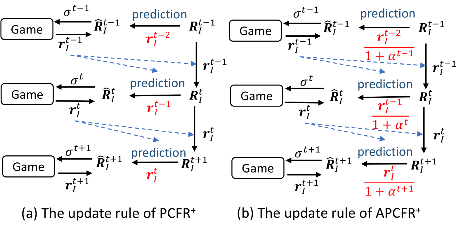
Figure 1: Comparison between the update rules of PCFR⁺ and APCFR⁺, with differences highlighted in red.

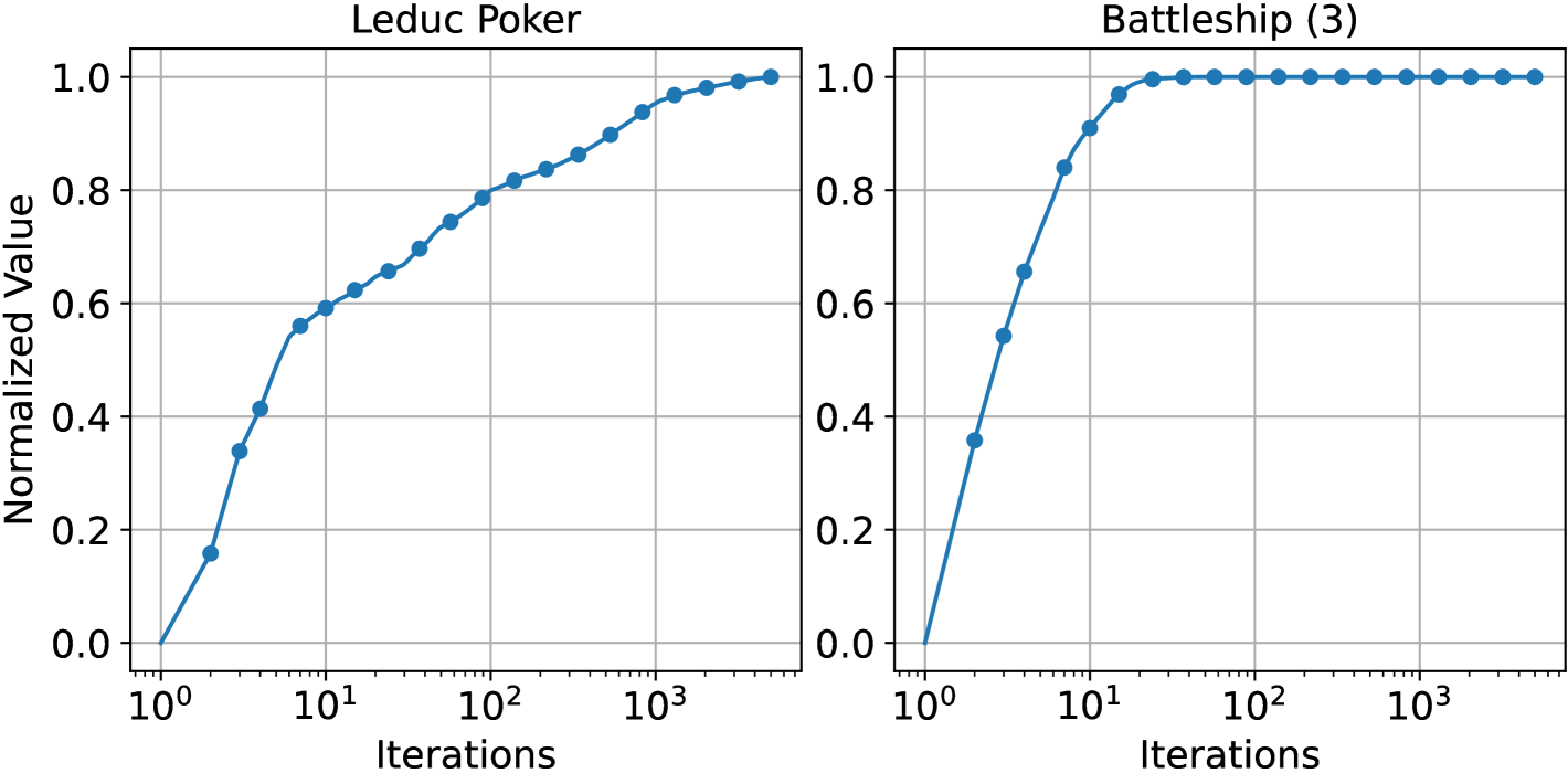
Figure 2: Dynamics of accumulated inaccuracy in PCFR⁺ between predicted and observed instantaneous counterfactual regrets in Leduc Poker and Battleship (3). This accumulated inaccuracy is related to theoretical convergence rate of PCFR⁺ (Theorem 4.1). The values on the y-axis are normalized to the range [0, 1].

To enhance the robustness of PCFR⁺, we propose a novel variant of PCFR⁺, termed Asynchronous PCFR⁺ (APCFR⁺). Similar to PCFR⁺, APCFR⁺ leverages the prediction to improve the convergence rate, but it mitigates the impact of the prediction inaccuracy on convergence. Specifically, as illustrated in Figure 1, APCFR⁺ utilizes an adaptive asynchronization mechanism for step-sizes between implicit and explicit accumulated counterfactual regret updates, which dynamically reduces the step-size when updating via the prediction. We prove that when the step-size for updating the explicit accumulated counterfactual regret via the prediction at iteration $t$ is set to ${1}/{(1+\alpha^{t})}$ for APCFR⁺, where $\alpha^{t}\geq 0$, the effect of the prediction inaccuracy on the convergence rate for APCFR⁺ is reduced by a factor of $1+\alpha^{t}$ compared to PCFR⁺. Therefore, APCFR⁺ mitigates the impact of the prediction inaccuracy on the convergence rate. Then, through the theoretical analysis of APCFR⁺, we propose an automatic learning mechanism for $\alpha^{t}$, eliminating the need for fine-tuning parameters across different games. To the best of our knowledge, we are the first to use different step-sizes for updating implicit and explicit accumulated counterfactual regrets.

We also introduce a simplified version of APCFR⁺, called Simple APCFR⁺ (SAPCFR⁺), which sets $\alpha^{t}$ as a constant to simplify the implementation that SAPCFR⁺ can be implemented with a single-line modification to the PCFR⁺ code. Notably, the constant is derived from the theoretical analysis of APCFR⁺, guaranteeing that SAPCFR⁺ achieves a constant-factor improvement in the worst-case theoretical convergence rate compared to PCFR⁺.

We conduct extensive experimental evaluations of APCFR⁺ across nine instances from five standard IIG benchmarks, including Kuhn Poker, Leduc Poker, Goofspiel, Liar’s Dice, and Battleship, as well as two heads-up no-limit Texas Hold’em (HUNL) Subgames generated by the top poker agent, Libratus (Brown & Sandholm, 2018). The experiments demonstrate that our algorithms outperforms PCFR⁺ in almost all tested games, and achieves an empirical convergence rate comparable to that of PCFR⁺ at a minimum. Moreover, we observe that SAPCFR⁺ achieves comparable empirical convergence rate with APCFR⁺.

2 Related Work

We focus on CFR algorithms (Zinkevich et al., 2007; Lanctot et al., 2009; Tammelin, 2014; Brown & Sandholm, 2019a; Farina et al., 2021, 2019; Liu et al., 2021; Pérolat et al., 2021; Liu et al., 2023; Meng et al., 2023; Farina et al., 2023; Xu et al., 2022, 2024b, 2024a; Zhang et al., 2024), the most widely used method for learning an NE in two-player zero-sum IIGs, as evidenced by their success in superhuman game AIs (Bowling et al., 2015; Moravč´ık et al., 2017; Brown & Sandholm, 2018, 2019b; Pérolat et al., 2022).

The key insight of CFR algorithms is the decomposition of the regret over the game into the sum of counterfactual regrets associated within infosets. The vanilla CFR algorithm, introduced by Zinkevich et al. (2007), employs RM (Hart & Mas-Colell, 2000) as the local regret minimizer. To improve the empirical convergence rate of CFR, it is common to design more effective local regret minimizers, as the selection of the local regret minimizers has a significant impact on the overall performance of the CFR algorithm. Examples include RM⁺ (Bowling et al., 2015), Discounted RM (DRM) (Brown & Sandholm, 2019a), and PRM⁺ (Farina et al., 2021), which correspond to CFR⁺ (Bowling et al., 2015), DCFR (Brown & Sandholm, 2019a), and PCFR⁺ (Farina et al., 2021), respectively. PCFR⁺ can demonstrate a extremely faster empirical convergence rate than other CFR variants. However, as shown in its original paper, PCFR⁺ is outperformed by CFR⁺ and DCFR even on standard IIG benchmarks like Leduc Poker and Liar’s Dice.

To improve the robustness of PCFR⁺, Farina et al. (2023) propose Stable PCFR⁺ and Smooth PCFR⁺. These algorithms improve the robustness by addressing the instability, i.e., rapid strategy fluctuations across iterations, via ensuring the lower bound of the 1-norm of accumulated counterfactual regrets exceeds a positive constant. However, these algorithms never outperform PCFR⁺ even they achieve a faster theoretical convergence rate than PCFR⁺. APCFR⁺ does not focus on addressing the instability, but instead aims to mitigate the impact of the prediction inaccuracy on the convergence to improve the robustness. In our experiments, APCFR⁺ consistently outperforms Stable PCFR⁺ and Smooth PCFR⁺ in all tested games.

3 Preliminaries

Imperfect-information Extensive-form games (IIGs). To model tree-form sequential decision-making problems with hidden information, a common used model is IIG (Osborne et al., 2004). An IIG can be formulated as $G=\{\mathcal{N},\mathcal{H},P,A,\mathcal{I},\{u_{i}\}\}$. Here, $\mathcal{N}=\{0,1\}$ is the set of players. “Nature” is also considered a player $c$ (representing chance) and chooses actions with a fixed known probability distribution. $\mathcal{H}$ is the set of all possible histories. For each history $h\in\mathcal{H}$, the function $P(h)$ represents the player acting at history $h$, and $A(h)$ denotes the actions available at history $h$. To account for private information, the histories for each player $i$ are partitioned into a collection $\mathcal{I}_{i}$, referred to as information sets (infosets). For any infoset $I\in\mathcal{I}_{i}$, histories $h,h^{\prime}\in I$ are indistinguishable to player $i$. The notation $\mathcal{I}$ denotes $\mathcal{I}=\{\mathcal{I}_{i}|i\in\mathcal{N}\}$. Thus, we have $P(I)=P(h)$, $A(I)=A(h),\forall h\in I$. The set of leaf nodes is denoted by $\mathcal{Z}$. For each leaf node $z$, there is a pair $(u_{0}(z),u_{1}(z))\in[-1,\ 1]$ which denotes the payoffs for the min player (player 0) and the max player (player 1) respectively. In two-player zero-sum IIGs, $u_{0}(z)=-u_{1}(z),\forall z\in\mathcal{Z}$.

Behavioral strategy. In this paper, we present the strategy via behavioral strategy. This strategy $\sigma_{i}$ is defined on each infoset. For any infoset $I\in\mathcal{I}_{i}$, the probability for an action $a\in A(I)$ is denoted by $\sigma_{i}(I,a)$. We use $\sigma_{i}(I)=[\sigma_{i}(I,a)|a\in A(I)]\in\Delta^{|A(I)|}$ to denote the strategy at infoset $I$, where $\Delta^{|A(I)|}$ is a $(|A(I)|-1)$-dimension simplex. If every player follows the strategy profile $\sigma=[\sigma_{0};\sigma_{1}]$ and reaches infoset $I$, the reaching probability is denoted by $\pi^{{\sigma}}(I)$. The contribution of $i$ to this probability is $\pi_{i}^{\sigma}(I)$ and $\pi_{-i}^{\sigma}(I)$ for other than $i$, where $-i$ denotes the players other than $i$. In IIGs, $u_{i}(\sigma_{i},\sigma_{-i})=\sum_{z\in\mathcal{Z}}u_{i}(z)\pi^{\sigma}(z)$.

Nash equilibrium (NE). NE denotes a rational behavior where no player can benefit by unilaterally deviating from the equilibrium. For any player, her strategy is the best-response to the strategies of others. Formally, for any NE strategy profile $\sigma^{*}$ and $i\in\mathcal{N}$, it holds that $u_{i}(\sigma^{*}_{i},\sigma^{*}_{-i})\geq u_{i}(\sigma_{i},\sigma^{*}_{-i})$ for all $\sigma$. A widely used metric to measure the distance from the given strategy profile $\bm{x}$ to NE is the exploitability, which is defined as $\epsilon(\sigma)=\sum_{i\in\mathcal{N}}\max_{\sigma^{\prime}_{i}}(u_{i}(\sigma_{i},\sigma_{-i})-u_{i}(\sigma^{\prime}_{i},\sigma_{-i}))/|\mathcal{N}|$. If $\epsilon(\sigma)=\delta$, then $\sigma$ is called as an $\delta$-NE.

Computing an NE via regret minimization algorithms. To compute an NE in IIGs, a common used method is regret minimization algorithms (Rakhlin & Sridharan, 2013a, b; Hazan et al., 2016; Joulani et al., 2017). For any sequence of strategies $\sigma_{i}^{1},\cdots,\sigma_{i}^{T}$ of player $i$, player $i$’s regret is $R^{T}_{i}=\max_{\sigma_{i}}\sum^{T}_{t=1}u_{i}(\sigma_{i},\sigma^{t}_{-i})-\sum^{T}_{t=1}u_{i}(\sigma^{t}_{i},\sigma^{t}_{-i})$ for all sequence $\sigma_{-i}^{1},\cdots,\sigma_{-i}^{T}$. Regret minimization algorithms are algorithms ensuring $R^{T}_{i}$ grows sublinearly. If each player follows a regret minimization algorithm, then their average strategy converges to the set of the NE in two-player zero-sum IIGs. Formally, assume the regret of each player $i$ is $R^{T}_{i}$, then it hods that

$$\footnotesize\epsilon(\bar{\sigma})=\epsilon(\bar{\sigma}_{0},\bar{\sigma}_{1})\leq\frac{\sum_{i\in\mathcal{N}}R^{T}_{i}}{|\mathcal{N}|T},$$ (1)

where $\bar{\sigma}_{i}(I)=\sum_{t=1}^{T}\pi^{\sigma^{t}}_{i}(I){\sigma^{t}_{i}}(I)/\sum_{t=1}^{T}\pi^{\sigma^{t}}_{i}(I)$ for all $i\in\mathcal{N}$ and $I\in\mathcal{I}_{i}$.

Counterfactual Regret Minimization (CFR) framework. This framework (Zinkevich et al., 2007; Farina et al., 2019; Liu et al., 2021; Farina et al., 2023) is designed to compute an NE of two-player zero-sum IIGs. Instead of directly minimizing the global regret, this framework decomposes the regret to each infoset and independently minimizes the local regret within each infoset. Let $\sigma^{t}$ be the strategy profile at iteration $t$. CFR algorithms compute the counterfactual value at infoset $I$ for action $a$ as

$$\footnotesize v^{\sigma^{t}}(Ia)=\sum_{h\in I}\sum_{z\in\mathcal{Z}_{ha}}\pi^{\sigma^{t}}_{-i}(h)\pi^{\sigma^{t}}(ha,z)u_{i}(z),$$ (2)

where $\pi^{\sigma^{t}}(ha,z)$ denotes the probability from $ha$ to $z$ if all players play according to $\sigma^{t}$ and $\mathcal{Z}_{ha}$ is the set of the leaf nodes that are reachable after choosing action $a$ at history $h$. For any infoset $I$, the counterfactual regret is

$$\footnotesize R^{T}(I)=\max_{a\in A(I)}\sum_{t=1}^{T}v^{\sigma^{t}}(Ia)-\sum_{t=1}^{T}\sum_{a\in A(I)}\sigma^{t}_{i}(Ia)v^{\sigma^{t}}(Ia).$$ (3)

Zinkevich et al. (2007) show that the regret over the game $R^{T}_{i}=\max_{\sigma_{i}}\sum^{T}_{t=1}u_{i}(\sigma_{i},\sigma^{t}_{-i})-\sum^{T}_{t=1}u_{i}(\sigma^{t}_{i},\sigma^{t}_{-i})$ is less than the sum of the counterfactual regrets within infosets:

$$\footnotesize R^{T}_{i}\leq\sum_{I\in\mathcal{I}_{i}}R^{T}(I).$$ (4)

So any regret minimization algorithms can be used as the local regret minimizer to minimize the regret $R^{T}(I)$ over each infoset to minimize the regret $R^{T}_{i}$.

Vanilla Counterfactual Regret Minimization (Vanilla CFR). The first CFR algorithm is proposed by Zinkevich et al. (2007), which uses Regret Matching (RM) (Hart & Mas-Colell, 2000; Gordon, 2006) as the local regret minimizer. Formally, at each iteration $t$, vanilla CFR updates its accumulated counterfactual regret ${\bm{R}}^{t}_{I}$ (notably, it is a vector while $R^{T}_{i}$ is a scalar) at infoset $I$ via

$${\bm{R}}^{t+1}_{I}={\bm{R}}^{t}_{I}+\bm{r}^{t}_{I},$$ (5)

where $\bm{r}^{t}_{I}=v^{\sigma^{t}}(I)-\langle v^{\sigma^{t}}(I),\sigma^{t}_{i}(I)\rangle\bm{1}$ is the instantaneous counterfactual regret. Then, vanilla CFR gets the new strategy via the regret-matching operator

$$\sigma^{t+1}_{i}(I)=\frac{[{\bm{R}}^{t+1}_{I}]^{+}}{\|[{\bm{R}}^{t+1}_{I}]^{+}\|_{1}},$$ (6)

where $i=P(I)$ and $[\cdot]^{+}=\max(\cdot,\bm{0})$.

Counterfactual Regret Minimization⁺ (CFR⁺). To improve the empirical convergence rate of vanilla CFR, Tammelin (2014) propose a variant of vanilla CFR called CFR⁺, which utilizes Regret Matching⁺ (RM⁺) (Tammelin, 2014) as the local regret minimizer. The key insight of RM⁺ is to ensure that ${\bm{R}}^{t}_{I}\geq\bm{0}$ at each iteration $t$ and infoset $I$. Formally, at each iteration $t$, CFR⁺ updates its accumulated counterfactual regret ${\bm{R}}^{t}_{I}$ at infoset $I$ according to

$${\bm{R}}^{t+1}_{I}=[{\bm{R}}^{t}_{I}+\bm{r}^{t}_{I}]^{+}.$$ (7)

Then, as done in CFR, CFR⁺ gets strategies via the regret-matching operator

$$\sigma^{t+1}_{i}(I)=\frac{[{\bm{R}}^{t+1}_{I}]^{+}}{\|[{\bm{R}}^{t+1}_{I}]^{+}\|_{1}}=\frac{{\bm{R}}^{t+1}_{I}}{\|{\bm{R}}^{t+1}_{I}\|_{1}},$$ (8)

where $i=P(I)$, and the second equality comes from the fact that ${\bm{R}}^{t+1}_{I}\geq\bm{0}$.

Predictive Counterfactual Regret Minimization⁺ (PCFR⁺). PCFR⁺ (Farina et al., 2021) is a powerful variant of CFR⁺. It significantly outperforms CFR⁺ in many IIGs. PCFR⁺ employs Predictive RM⁺ (PRM⁺) (Farina et al., 2021) as its local regret minimizer, with its key insight is to use the prediction. Specifically, as shown Figure 1, at each iteration $t$, PCFR⁺ maintains implicit and explicit accumulated counterfactual regrets: ${\bm{R}}^{t}_{I}$ and $\hat{\bm{R}}^{t-1}_{I}$. Firstly, PCFR⁺ makes a prediction and uses this prediction to derive new explicit accumulated counterfactual regrets $\hat{\bm{R}}^{t}_{I}$ from ${\bm{R}}^{t}_{I}$. Then, PCFR⁺ observes the instantaneous counterfactual regret $\bm{r}^{t}_{I}$ by following the strategy $\sigma^{t}$ defined by $\hat{\bm{R}}^{t}_{I}$. Lastly, $\bm{r}^{t}_{I}$ is subsequently used to derive ${\bm{R}}^{t+1}_{I}$ from ${\bm{R}}^{t}_{I}$. If the prediction aligns with the observed instantaneous counterfactual regret $\bm{r}^{t}_{I}$, Farina et al. (2021) show that the theoretical convergence of PCFR⁺ can be improved from $O(1/\sqrt{T})$ of CFR⁺ to $O(1/T)$. As tested in Farina et al. (2021), using the instantaneous counterfactual regret $\bm{r}^{t-1}_{I}$ observed at the previous iteration $t-1$ as the prediction is both simple and effective. Therefore, in practice, PCFR⁺ uses $\bm{r}^{t-1}_{I}$ as the prediction at iteration $t$. Formally, at each iteration $t$ and for each infoset $I\in\mathcal{I}$, PCFR⁺ updates its strategy according to

$$\hat{\bm{R}}^{t}_{I}=[{\bm{R}}^{t}_{I}+\bm{r}^{t-1}_{I}]^{+},{\bm{R}}^{t+1}_{I}=[{\bm{R}}^{t}_{I}+\bm{r}^{t}_{I}]^{+},\$$ (9)

$$\sigma^{t}_{i}(I)=\frac{[\hat{\bm{R}}^{t}_{I}]^{+}}{\|[\hat{\bm{R}}^{t}_{I}]^{+}\|_{1}}=\frac{\hat{\bm{R}}^{t}_{I}}{\|\hat{\bm{R}}^{t}_{I}\|_{1}},$$

where $i=P(I)$, ${\bm{R}}^{1}_{I}=\bm{0}$, and the second equality of the second line comes from the fact that $\hat{\bm{R}}^{t+1}_{I}\geq\bm{0}$.

4 Our Algorithms

PCFR⁺ leverages the prediction to accelerate the empirical convergence rate. However, when the prediction is inaccurate, its empirical convergence rate may decrease significantly, leading to unstable performance on certain IIGs. To enhance the robustness of PCFR⁺, in Section 4.1, we propose Asynchronous PCFR⁺ (APCFR⁺), which mitigates the impact of the prediction inaccuracy on convergence. We then provide a theoretical analysis for APCFR⁺ to demonstrate the reason why it enhances the robustness. Finally, we introduce Simple APCFR⁺ (SAPCFR⁺), a simple version of APCFR⁺, which requires only a single-line modification to the PCFR⁺ implementation, as detailed in Section 4.2. We show that SAPCFR⁺ achieves a constant-factor improvement in the theoretical convergence rate over PCFR⁺ in the worst case.

4.1 Asynchronou PCFR⁺ (APCFR⁺)

To mitigate the impact of the prediction inaccuracy on convergence of PCFR⁺, APCFR⁺ adaptively reduces the step-size when updating via the prediction, i.e., when updating the explicitly accumulated counterfactual regret. In other words, APCFR⁺ exploits the asynchrony of step-sizes between the updates of the implicit and explicit ones. Formally, at iteration $t$, the update rule of APCFR⁺ at infoset $I$ is

$$\hat{\bm{R}}^{t}_{I}=[{\bm{R}}^{t}_{I}+\frac{1}{1+\alpha^{t}_{I}}\bm{r}^{t-1}_{I}]^{+},{\bm{R}}^{t+1}_{I}=[{\bm{R}}^{t}_{I}+\bm{r}^{t}_{I}]^{+},\$$ (10)

$$\sigma^{t}_{i}(I)=\frac{[\hat{\bm{R}}^{t}_{I}]^{+}}{\|[\hat{\bm{R}}^{t}_{I}]^{+}\|_{1}}=\frac{\hat{\bm{R}}^{t}_{I}}{\|\hat{\bm{R}}^{t}_{I}\|_{1}},$$

where $i=P(I)$, ${\bm{R}}^{1}_{I}=\bm{0}$, and $\bm{r}^{0}_{I}=\bm{0}$. The comparison between the update rules of PCFR⁺ and APCFR⁺ has been shown in Figure 1. In the rest of this subsection, we first present the regret upper bound for APCFR⁺ with respect to any $\alpha^{t}_{I}$, as stated in Theorem 4.1. According to the discussion about Theorem 4.1, we show why APCFR⁺ can enhance the robustness of PCFR⁺ by mitigating the impact of the prediction inaccuracy on convergence. Lastly, we discuss how to automatically learn $\alpha^{t}_{I}$ from the regret bound shown in Theorem 4.1.

Theorem 4.1.

[Proof is in Appendix A]. Assuming that $T$ iterations of APCFR⁺ with any $\alpha^{t}_{I}\geq 0$ are conducted, the counterfactual regret at any infoset $I\in\mathcal{I}$ is bound by

$$\footnotesize R^{T}(I)\leq\sqrt{{\sum^{T}_{t=1}\left(\frac{\|{\bm{r}}^{t}_{I}-\bm{r}^{t-1}_{I}\|^{2}_{2}}{1+\alpha^{t}_{I}}+\alpha^{t}_{I}\|{\bm{R}}^{t+1}_{I}-{\bm{R}}^{t}_{I}\|^{2}_{2}\right)}}.$$

According to Theorem 4.1, APCFR⁺ mitigates the impact of the prediction inaccuracy, $\|{\bm{r}}^{t}_{I}-\bm{r}^{t-1}_{I}\|^{2}_{2}$, on the regret upper bound (the theoretical convergence rate) by introducing the term $\alpha^{t}_{I}\|{\bm{R}}^{t+1}_{I}-{\bm{R}}^{t}_{I}\|^{2}_{2}$. This reduces the impact of the prediction inaccuracy on the regret upper bound compared to PCFR⁺ by a factor of $1/(1+\alpha^{t}_{I})$ (note that when $\alpha^{t}_{I}=0$, APCFR⁺ reduces to PCFR⁺).

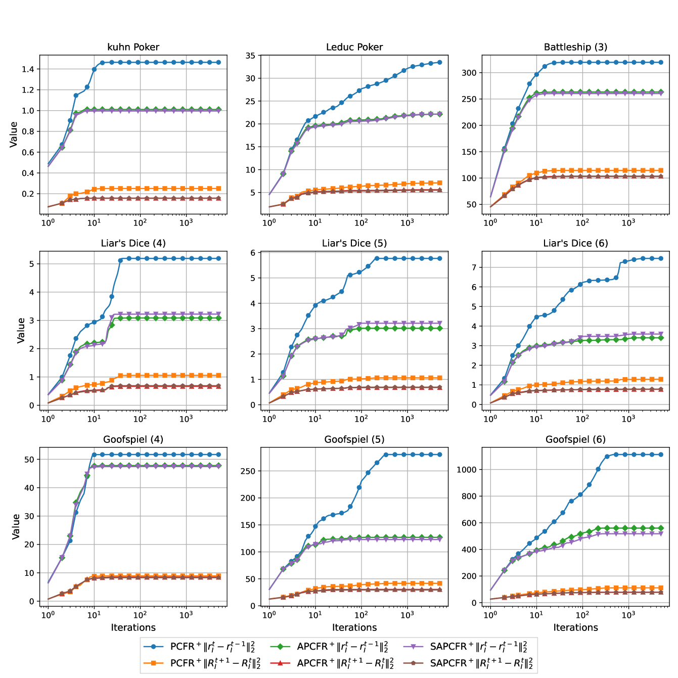
Figure 8: Dynamics of $\sum^{T}_{t=1}\|{\bm{r}}^{t}_{I}-{\bm{r}}^{t-1}_{I}\|^{2}_{2}$ and $\sum^{T}_{t=1}\|{\bm{R}}^{t+1}_{I}-{\bm{R}}^{t}_{I}\|^{2}_{2}$ in standard commonly used IIG benchmarks.

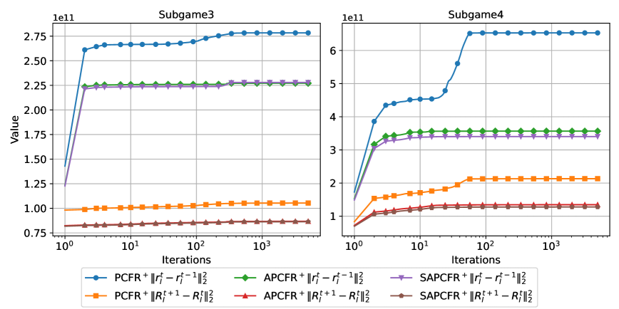
Figure 9: Dynamics of $\sum^{T}_{t=1}\|{\bm{r}}^{t}_{I}-{\bm{r}}^{t-1}_{I}\|^{2}_{2}$ and $\sum^{T}_{t=1}\|{\bm{R}}^{t+1}_{I}-{\bm{R}}^{t}_{I}\|^{2}_{2}$ in standard commonly used IIG benchmarks.

To assess the effectiveness of the asynchronization mechanism for step-sizes in decreasing the regret upper bound, we first present an example to show $\|{\bm{r}}^{t}_{I}-\bm{r}^{t-1}_{I}\|^{2}_{2}\geq\|{\bm{R}}^{t+1}_{I}-{\bm{R}}^{t}_{I}\|^{2}_{2}$. Assume that, the number of actions at infoset $I$ is $2$, ${\bm{R}}^{t}_{I}$ is $[1;0]$, as well as $\bm{r}^{t-1}_{I}$ and $\bm{r}^{t}_{I}$ are $[1;-1]$ and $[-1;1]$, respectively. From the update rule of PCFR⁺, we can derive that ${\bm{R}}^{t+1}_{I}=[{\bm{R}}^{t}_{I}+\bm{r}^{t}_{I}]^{+}=[0;1]$. Then, we have $\|{\bm{r}}^{t}_{I}-\bm{r}^{t-1}_{I}\|^{2}_{2}=8>\|{\bm{R}}^{t+1}_{I}-{\bm{R}}^{t}_{I}\|^{2}_{2}=2$. This phenomenon can be explained by fact that the upper bound of $\|{\bm{R}}^{t+1}_{I}-{\bm{R}}^{t}_{I}\|^{2}_{2}$ is only a quarter of the upper bound of $\|{\bm{r}}^{t}_{I}-\bm{r}^{t-1}_{I}\|^{2}_{2}$, which is also used to derive SAPCFR⁺ (detailed in Section 4.2). In experiments, we also analyze the values of two terms $\sum^{T}_{t=1}\|{\bm{r}}^{t}_{I}-\bm{r}^{t-1}_{I}\|^{2}_{2}\ \text{and}\sum^{T}_{t=1}\|{\bm{R}}^{t+1}_{I}-{\bm{R}}^{t}_{I}\|^{2}_{2},$ for both PCFR⁺ and our algorithms (Figures 8 and 9). Among all algorithms, we observe that the value of $\sum^{T}_{t=1}\|{\bm{r}}^{t}_{I}-\bm{r}^{t-1}_{I}\|^{2}_{2}$ is at least three times than that of $\sum^{T}_{t=1}\|{\bm{R}}^{t+1}_{I}-{\bm{R}}^{t}_{I}\|^{2}_{2}$. This indicates that introducing the term $\sum^{T}_{t=1}\alpha^{t}_{I}\|{\bm{R}}^{t+1}_{I}-{\bm{R}}^{t}_{I}\|^{2}_{2}$ and modifying the term $\sum^{T}_{t=1}\|{\bm{r}}^{t}_{I}-\bm{r}^{t-1}_{I}\|^{2}_{2}$ to $\sum^{T}_{t=1}\frac{\|{\bm{r}}^{t}_{I}-\bm{r}^{t-1}_{I}\|^{2}_{2}}{1+\alpha^{t}_{I}}$, can reduce the regret upper bound. Furthermore, compared to PCFR⁺, both these two terms are smaller in our algorithms, further decreasing the regret upper bound. Then, we evaluate the values of ${\sum^{T}_{t=1}(\frac{\|{\bm{r}}^{t}_{I}-{\bm{r}}^{t-1}_{I}\|^{2}_{2}}{1+\alpha^{t}_{I}}+\alpha^{t}_{I}\|{\bm{R}}^{t+1}_{I}-{\bm{R}}^{t}_{I}\|^{2}_{2})},$ for both PCFR⁺ and our algorithms (Figures 10 and 11). In all games, the value of $\sum^{T}_{t=1}(\frac{\|{\bm{r}}^{t}_{I}-{\bm{r}}^{t-1}_{I}\|^{2}_{2}}{1+\alpha^{t}_{I}}+\alpha^{t}_{I}\|{\bm{R}}^{t+1}_{I}-{\bm{R}}^{t}_{I}\|^{2}_{2})$ is consistently smaller in our algorithms than in PCFR⁺. See more details and discussions in Appendix D.

Notably, Theorem 4.1 does not conflict the upper regret bound of CFR⁺ (where $\alpha^{t}_{I}\to\infty$), as it provides a larger upper regret bound than the original CFR⁺ upper bound. By altering the proof method, we get $R^{T}(I)\leq\sqrt{\sum^{T}_{t=1}\|{\bm{r}}^{t}_{I}-\frac{1}{1+\alpha^{t}_{I}}\bm{r}^{t-1}_{I}\|^{2}_{2}}$ (detailed in Appendix B). By setting $\alpha^{t}_{I}\to\infty$, the original bound of CFR⁺ can be recovered. Additionally, for PCFR⁺ (where $\alpha^{t}_{I}\to 0$), the bound in Theorem 4.1 is identical to the one in its original version (the result in Theorem 3 of the original PCFR⁺ version can be easily improved to the bound presented in Theorem 4.1).

To eliminate the fine-tuning of $\alpha^{t}_{I}$, we propose an automated learning approach for $\alpha^{t}_{I}$. From Theorem 4.1, we have

$$R^{T}(I) \leq\sqrt{{\sum^{T}_{t=1}\left(\frac{\|\bm{r}^{t}_{I}-\bm{r}^{t-1}_{I}\|^{2}_{2}}{1+\alpha^{t}_{I}}+\alpha^{t}_{I}\|\bm{R}^{t+1}_{I}-\bm{R}^{t}_{I}\|^{2}_{2}\right)}}$$ (11)

$$\leq\sqrt{{\sum^{T}_{t=1}\left(\frac{\|\bm{r}^{t}_{I}-\bm{r}^{t-1}_{I}\|^{2}_{2}}{\alpha^{t}_{I}}+\alpha^{t}_{I}\|\bm{R}^{t+1}_{I}-\bm{R}^{t}_{I}\|^{2}_{2}\right)}}.$$

To minimize the second line in the above equation, we can set $\alpha^{t}_{I}=\sqrt{{\|\bm{r}^{t}_{I}-\bm{r}^{t-1}_{I}\|^{2}_{2}}/{\|\bm{R}^{t+1}_{I}-\bm{R}^{t}_{I}\|^{2}_{2}}}.$ However, this is not feasible, as we need $\alpha^{t}_{I}$ to compute $\bm{r}^{t}_{I}$. Therefore, we adopt an alternative approach: at each iteration $t$,

$$\alpha^{t}_{I}=\min\left(\sqrt{\frac{\sum_{\tau=1}^{t-1}\|\bm{r}^{\tau}_{I}-\bm{r}^{\tau-1}_{I}\|^{2}_{2}}{\sum_{\tau=1}^{t-1}\|\bm{R}^{\tau+1}_{I}-\bm{R}^{\tau}_{I}\|^{2}_{2}}},\ 5\right).$$ (12)

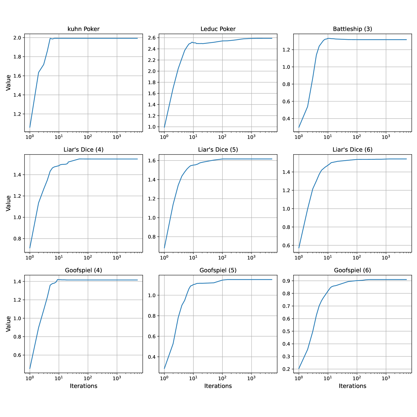
Figure 6: Dynamics of $\alpha^{t}_{I}$ in standard commonly used IIG benchmarks. Note that, contrary to figures in the main text, the x-axis in this figure is on a logarithmic scale, while the y-axis is not.

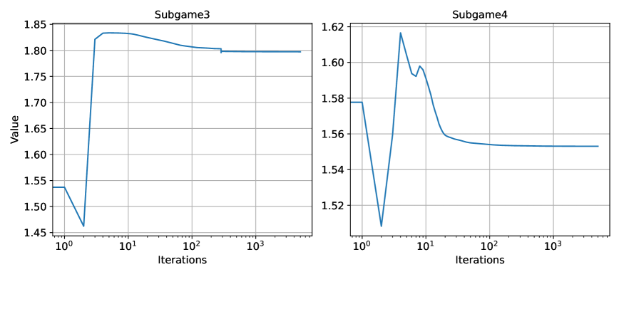
Figure 7: Dynamics of $\alpha^{t}_{I}$ in HUNL Subgames.

Note that $5$ in Eq. (12) is included solely to ensure that the bound in Theorem 4.1 remains finite. In practice, we rarely observed $\alpha^{t}_{I}$ reaching 5 (Figures 6 and 7).

4.2 Simple APCFR⁺ (SAPCFR⁺)

We now introduce SAPCFR⁺, which is implemented with a single-line modification to the PCFR⁺ code. Specifically, SAPCFR⁺ sets $\alpha^{t}_{I}$ as a constant. To determine an appropriate $\alpha^{t}_{I}$, we use a value that ensures SAPCFR⁺ achieves a constant-factor reduction in the regret bound compared to PCFR⁺ in the worst case. Formally, as previously discussed, the key insight of finding such $\alpha^{t}_{I}$ lies in the fact that the upper bound of $\|{\bm{R}}^{t+1}_{I}-{\bm{R}}^{t}_{I}\|^{2}_{2}$ is only a quarter of the upper bound of $\|{\bm{r}}^{t}_{I}-\bm{r}^{t-1}_{I}\|^{2}_{2}$ (details are in the following). Formally, we first present Lemma 4.2.

Lemma 4.2.

[Adapted from Lemma 11 of Wei et al. (2021)]. Assume that $T$ iterations of APCFR⁺ with any $\alpha^{t}_{I}\geq 0$ are conducted. Then for any infoset $I\in\mathcal{I}$ and $t\geq 1$, we have

$$\footnotesize\|{\bm{R}}^{t+1}_{I}-{\bm{R}}^{t}_{I}\|^{2}_{2}\leq\|{\bm{r}}^{t}_{I}\|^{2}_{2}.$$

Assume that for any infoset $I\in\mathcal{I}$ and $t\geq 1$, $\|{\bm{r}}^{t}_{I}\|^{2}_{2}\leq E$. Then, from Lemma 4.2, we have

$$\|{\bm{R}}^{t+1}_{I}-{\bm{R}}^{t}_{I}\|^{2}_{2}\leq E.$$ (13)

Similarly, for $\|{\bm{r}}^{t}_{I}-\bm{r}^{t-1}_{I}\|^{2}_{2}$, we have

$$\|{\bm{r}}^{t}_{I}-\bm{r}^{t-1}_{I}\|^{2}_{2}\leq 4E.$$ (14)

Combining Theorem 4.1, Eq. (13), and Eq. (14), in the worst case, we obtain

$$R^{T}(I) \leq\sqrt{{\sum^{T}_{t=1}\left(\frac{\|\bm{r}^{t}_{I}-\bm{r}^{t-1}_{I}\|^{2}_{2}}{1+\alpha^{t}_{I}}+\alpha^{t}_{I}\|\bm{R}^{t+1}_{I}-\bm{R}^{t}_{I}\|^{2}_{2}\right)}}$$ (15)

$$\leq\sqrt{{\sum^{T}_{t=1}\left(\frac{4E}{1+\alpha^{t}_{I}}+\alpha^{t}_{I}E\right)}}.$$

It is evident that when $\alpha^{t}_{I}=0$, i.e., for PCFR⁺, the worst-case counterfactual regret upper bound is given by

$$R^{T}(I) \leq\sqrt{\sum^{T}_{t=1}4E}.$$ (16)

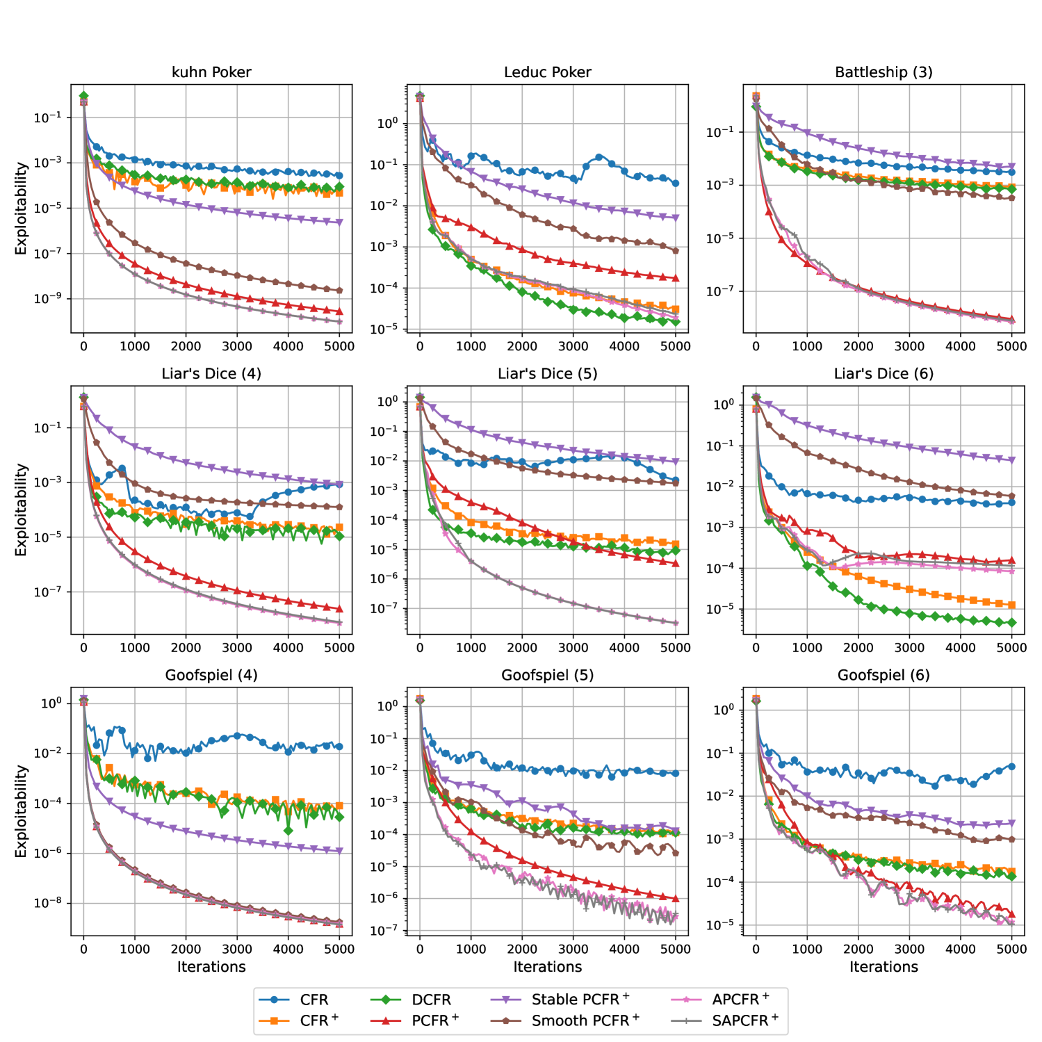
Figure 3: Empirical convergence for CFR, CFR⁺, DCFR, PCFR⁺, Stable PCFR⁺, Smooth PCFR⁺, APCFR⁺, and SAPCFR⁺ in standard commonly used IIG benchmarks. Each algorithm runs for 5,000 iterations. In all plots,the x-axis is the number of iteration, and the y-axis represents exploitability,displayed on a logarithmic scale. Liar’s Dice ($x$) represents that every player is given a die with $x$ sides. Goofspiel ($x$) denotes that each player is dealt $x$ cards. Battleship ($x$) implies the size of grids is $x$.

When we set $\alpha^{t}_{I}=2$ (which comes from facts that (i) $2$ minimizes ${{\sum^{T}_{t=1}({4E}/{\alpha^{t}_{I}}+\alpha^{t}_{I}E)}}$ for any positive $E$ and (ii) ${{\sum^{T}_{t=1}({4E}/{(1+\alpha^{t}_{I})}+\alpha^{t}_{I}E)}}\leq{{\sum^{T}_{t=1}({4E}/{\alpha^{t}_{I}}+\alpha^{t}_{I}E)}}$), the counterfactual regret is bound by

$$R^{T}(I) \leq\sqrt{\sum^{T}_{t=1}\left(\frac{4E}{1+2}+2E\right)}=\sqrt{\sum^{T}_{t=1}\frac{10E}{3}}.$$ (17)

Clearly, setting $\alpha^{t}_{I}=2$ results in a lower regret upper bound. Therefore, for SAPCFR⁺, we set $\alpha^{t}_{I}=2$ for all $t\geq 1$. Formally, at each iteration $t$, SAPCFR⁺ updates its strategy at each infoset $I\in\mathcal{I}$ according to the following update rule:

$$\hat{\bm{R}}^{t}_{I}=[{\bm{R}}^{t}_{I}+\frac{1}{3}\bm{r}^{t-1}_{I}]^{+},\ {\bm{R}}^{t+1}_{I}=[{\bm{R}}^{t}_{I}+\bm{r}^{t}_{I}]^{+},$$ (18)

$$\sigma^{t}_{i}(I)=\frac{[\hat{\bm{R}}^{t}_{I}]^{+}}{\|[\hat{\bm{R}}^{t}_{I}]^{+}\|_{1}}=\frac{\hat{\bm{R}}^{t}_{I}}{\|\hat{\bm{R}}^{t}_{I}\|_{1}},$$

where $i=P(I)$, ${\bm{R}}^{1}_{I}=\bm{0}$, and $\bm{r}^{0}_{I}=\bm{0}$.

5 Experiments

We now evaluate the empirical convergence rates of our algorithms, APCFR⁺ and SAPCFR⁺. Additional experiments on (i) the dynamics of $\alpha^{t}_{I}$ in APCFR⁺, and (ii) the dynamics of these terms: $\sum_{t=1}^{T}\|\bm{r}^{t}_{I}-\bm{r}^{t-1}_{I}\|^{2}_{2},\ \sum_{t=1}^{T}\|\bm{R}^{t+1}_{I}-\bm{R}^{t}_{I}\|^{2}_{2}$, and $\sum_{t=1}^{T}(\frac{\|\bm{r}^{t}_{I}-\bm{r}^{t-1}_{I}\|^{2}_{2}}{1+\alpha^{t}_{I}}+\alpha^{t}_{I}\|\bm{R}^{t+1}_{I}-\bm{R}^{t}_{I}\|^{2}_{2})$ for APCFR⁺, SAPCFR⁺, and PCFR⁺, are in Appendix D. The results in Appendix D show that, for these terms, their values are smaller in our algorithms compared to PCFR⁺.

Configurations. Our evaluation includes a comparison with several existing PCFR⁺ variants as well as other classical CFR algorithms. Specifically, we compare APCFR⁺ and SAPCFR⁺ against PCFR⁺ (Farina et al., 2021), Stable PCFR⁺ (Farina et al., 2023), Smooth PCFR⁺ (Farina et al., 2023), vanilla CFR (Zinkevich et al., 2007), CFR⁺ (Tammelin, 2014), and DCFR (Brown & Sandholm, 2019a). Each algorithm is run for 5000 iterations, which is sufficient to achieve low exploitability in the tested games. As done in the original PCFR⁺ version, we employ alternating updates and quadratic averaging for APCFR⁺, SAPCFR⁺, Stable PCFR⁺, and Smooth PCFR⁺. In addition, for Stable PCFR⁺ and Smooth PCFR⁺, we set their step-sizes to 1, the configuration of their original versions. All experiments are conducted on a machine with a Xeon(R) Gold 6444Y CPU and 256 GB of memory.

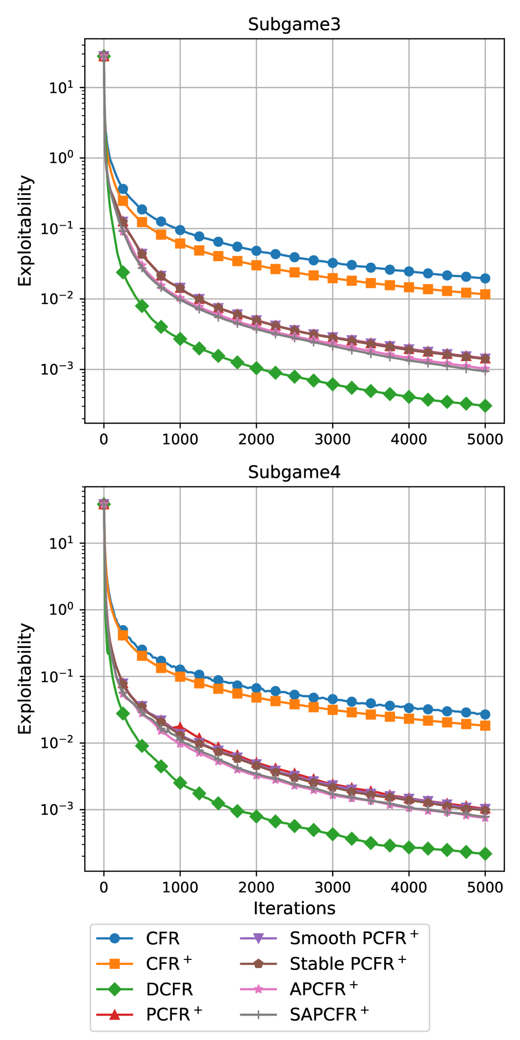
Figure 4: Empirical convergence for CFR, CFR⁺, DCFR, PCFR⁺, Stable PCFR⁺, Smooth PCFR⁺, APCFR⁺, and SAPCFR⁺ in HUNL Subgames. Notably, the final exploitability of our algorithms in both subgames is approximately $70\%$ of that of PCFR⁺.

Empirical convergence rates in standard IIG benchmarks. We now present the empirical convergence rates across five standard IIG benchmarks, namely, Kuhn Poker, Leduc Poker, Goofspiel Poker, Liar’s Dice, and Battleship. All the games are implemented using OpenSpiel (Lanctot et al., 2019). The algorithm implementations are based on the open-source code of LiteEFG (Liu et al., 2024), as LiteEFG provides a significant speedup—approximately 100 times faster in executing the same number of iterations compared to the default implementation in OpenSpiel. The experimental results are shown in Figure 3. We observe that, for most of the tested games, except for Battleship ($3$) and Goofspiel ($4$), our algorithms, APCFR⁺ and SAPCFR⁺, significantly outperform PCFR⁺. Even in Battleship ($3$) and Goofspiel ($4$), APCFR⁺ and SAPCFR⁺ demonstrate performance similar to that of PCFR⁺, achieving the similar exploitability after 5000 iterations. In fact, based on the experimental results in Appendix D (Figures 8 and 9), we observe that the games, such as Battleship (3) and Goofspiel (4), where our algorithms do not show an improvement over PCFR⁺ are also games where PCFR⁺ exhibits a rapid decrease in the inaccuracy between the predicted and observed instantaneous counterfactual regrets (detailed discussions are provided in Appendix D). Furthermore, the performance gap between APCFR⁺ and SAPCFR⁺ is relatively small. Specifically, APCFR⁺ is only slightly outperforms SAPCFR⁺ in Leduc Poker, Battleship (3), Liar’s Dice (5), and Liar’s Dice (6). This small performance gap means that in practical applications, SAPCFR⁺ can be directly used due to its ease of implementation and a faster convergence rate compared to PCFR⁺. Regarding other variants of PCFR⁺, namely Stable PCFR⁺ and Smooth PCFR⁺, we find that their empirical convergence performance significantly lags behind that of PCFR⁺. Additionally, compared to other classical CFR algorithms, our algorithms significantly outperform vanilla CFR in all games. Moreover, compared CFR⁺ and DCFR, our algorithms significantly outperform them in all games except Leduc Poker and Liar’s Dice ($6$). In fact, with an increased number of iterations, our algorithms would likely surpass these classical CFR algorithms even in Leduc Poker.

Empirical convergence rates in HUNL Subgames. We evaluate the empirical convergence rate in HUNL Subgames, which are significantly larger than the standard IIG benchmarks tested (see Appendix D for details). Since OpenSpiel does not support HUNL Subgames, we utilize Poker RL (Steinberger, 2019). More precisely, our code are based on the code from (Xu et al., 2024b). The code in (Xu et al., 2024b) supports only Subgame 3 and Subgame 4, so we conduct experiments solely on these two HUNL Subgames. The results are shown in Figure 4. As observed in the standard IIG benchmark experiments, our algorithms, APCFR⁺ and SAPCFR⁺, outperform PCFR⁺ in both subgames. In fact, our algorithms exceed all others, except DCFR, in both subgames. Although our algorithms do not outperform DCFR, it is worth noting that no other algorithm surpasses DCFR, whose parameters are specifically fine-tuned for HUNL Subgames. Our method and DCFR are not mutually exclusive and can be combined. Specifically, the core idea of our algorithm—the asynchronization of step-sizes between the updates of implicit and explicit accumulated counterfactual regrets—can be integrated with DCFR’s approach, which discounts prior iterations when calculating accumulated regrets. Consequently, we apply the asynchronization mechanism for step-sizes to enhance PDCFR⁺ (Xu et al., 2024b), a combination of DCFR and PCFR⁺, resulting in APDCFR⁺. Notably, APDCFR⁺ employs a novel aggressive discount weighting scheme for computing accumulated regrets, differing from the scheme used in the original PDCFR⁺. The experimental results are presented in Figure 5. APDCFR⁺ significantly outperforms both PDCFR⁺ and APCFR⁺, and even surpasses DCFR in Subgame 3. Then, we combine APDCFR⁺ with Stable PCFR⁺ to form Stable APDCFR⁺, further improving performance, and surpassing DCFR in both HUNL Subgames. We also test the combinations of Stable PCFR⁺ with PDCFR⁺ and APCFR⁺, denoted as Stable PDCFR⁺ and Stable APCFR⁺, respectively. However, Stable PDCFR⁺ and Stable APCFR⁺ even will fall short of PDCFR⁺ and APCFR⁺, respectively, let alone Stable APDCFR⁺, indicating that each component in Stable APDCFR⁺ is crucial. We also evaluate Stable SAPDCFR⁺, the combination of Stable PCFR⁺, PDCFR⁺, and SAPCFR⁺. We observe that Stable SAPDCFR⁺ underperforms Stable APDCFR⁺ in both subgames. Thus, we present only the Stable APDCFR⁺. Details of APDCFR⁺ and Stable APDCFR⁺ are in Appendix C.

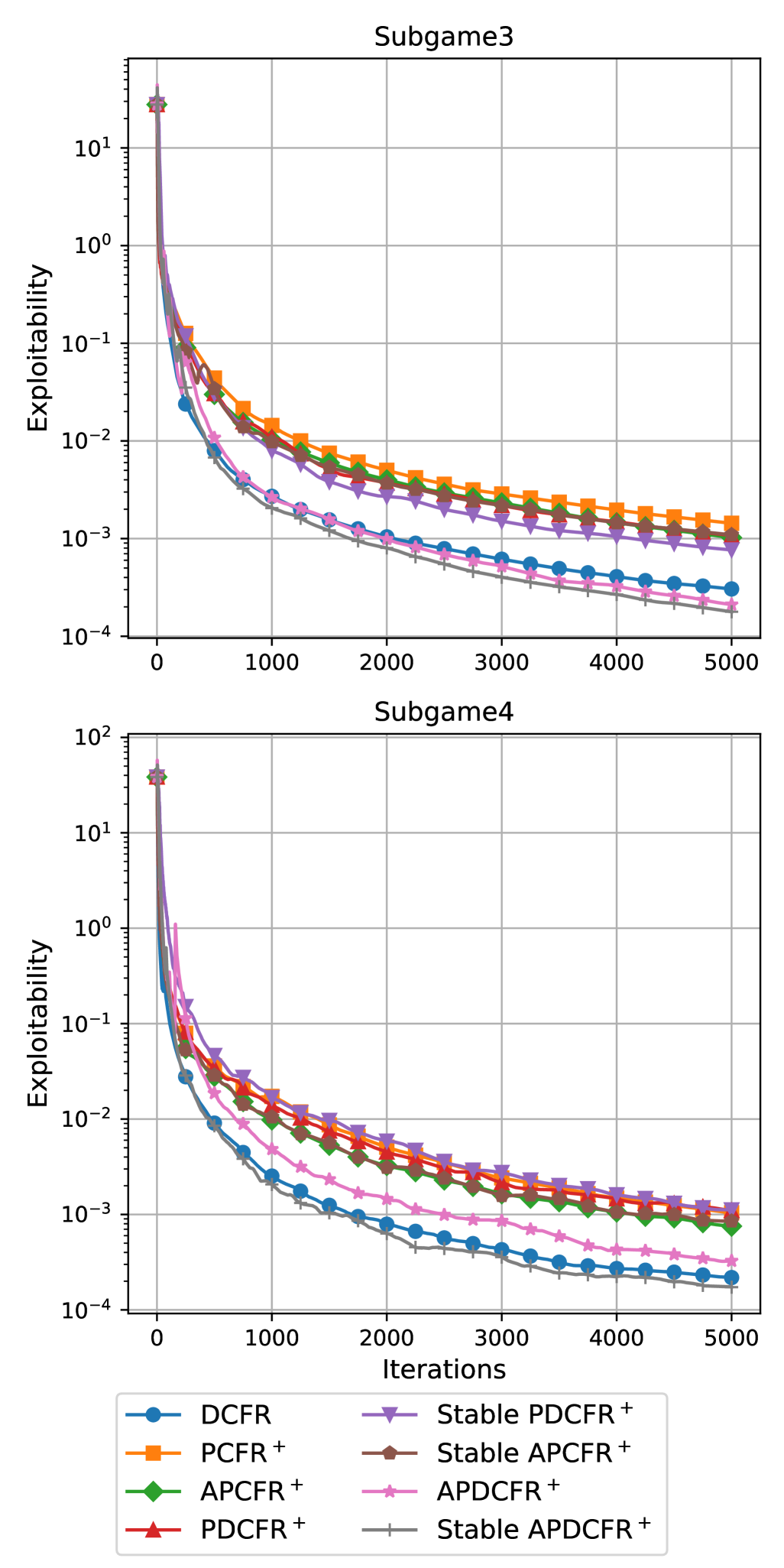
Figure 5: Empirical convergence for DCFR, PCFR⁺, PDCFR⁺, APCFR⁺, PDCFR⁺, Stable APCFR⁺, Stable PDCFR⁺, APDCFR⁺, and Stable APDCFR⁺ in HUNL Subgames.

Table 1: Comparison of running times (in minutes).

	PCFR+	APCFR+	SAPCFR+
kuhn Poker	0.0020	0.0033	0.0021
Leduc Poker	0.4252	0.6423	0.4408
Battleship (3)	50.1909	58.4390	50.8602
Liar’s Dice (4)	0.4327	0.5690	0.4308
Liar’s Dice (5)	3.8178	4.0365	3.7922
Liar’s Dice (6)	22.8226	24.7680	22.2554
Goofspiel (4)	0.0290	0.0393	0.0279
Goofspiel (5)	0.9323	1.9760	0.9430
Goofspiel (6)	52.4023	56.2751	51.7243
Subgame3	278.7428	297.3784	276.9873
Subgame4	245.1753	254.4792	249.0042

Running times. We now compare the running time of our algorithms with that of PCFR⁺, both executed with the same number of iterations (i.e., 5000). The experimental results are shown in Table 1. We observe that the running time of APCFR⁺ is higher compared to PCFR⁺, primarily due to the additional $\alpha^{t}_{I}$ learning process in APCFR⁺, which increases its running time. However, we also note that the running time of SAPCFR⁺ is nearly identical to that of PCFR⁺, as the only difference between their implementations is a single line of code, which does not alter the computational complexity. Importantly, the computational complexity remains exactly the same, even with no change in the constant factors.

6 Conclusions

We propose APCFR⁺, a novel variant of PCFR⁺. APCFR⁺ employs the asynchronization of step-sizes in the updates of implicit and explicit accumulated counterfactual regrets to make a more conservative prediction than PCFR⁺. This conservative prediction reduces the the impact of the prediction inaccuracy, which typically slows down the convergence rate of PCFR⁺, to improve the robustness. In addition, we introduce SAPCFR⁺, requiring only a single line modification to PCFR⁺. Experimental results validate that APCFR⁺ and SAPCFR⁺ exhibit a faster empirical convergence rate than PCFR⁺. To the best of our knowledge, we are the first to propose the asynchronization of step-sizes in the updates of implicit and explicit accumulated counterfactual regrets, a simple yet novel technique that effectively improves the robustness of PCFR⁺.

Moreover, the techniques used in other PCFR⁺ variants are compatible with our algorithm. By integrating the techniques from other PCFR⁺ variants, we introduce APDCFR⁺ and Stable APDCFR⁺, which further improve the empirical convergence rate of APCFR⁺ in HUNL Subgames.

Impact Statement

This paper presents work whose goal is to advance the field of Machine Learning. There are many potential societal consequences of our work, none which we feel must be specifically highlighted here.

Appendix A Proof of Theorem 4.1

Proof.

To prove Theorem 4.1, we use the equivalence between RM⁺ and Online Mirror Descent (OMD) proposed by Farina et al. (2021). We first introduce OMD. OMD is a traditional regret minimization algorithm (Nemirovskij & Yudin, 1983). Let $\bm{\ell}^{t}\in\mathbb{R}^{d}$, $\bm{x}^{t}\in\mathcal{D}$, and let $\psi:\mathcal{D}\to\mathbb{R}^{d}_{\geq 0}=\{\bm{y}|\bm{y}\in\mathbb{R}^{d},\bm{y}\geq\bm{0}\}$ be a 1-strongly convex differentiable regularizer with respect to some norm $\|\cdot\|$, OMD generates the decisions via

$$\small\bm{x}^{t+1}:=\arg\min_{\bm{x}^{\prime}\in\mathcal{D}}\left\{\langle\bm{\ell}^{t},\bm{x}^{\prime}\rangle+\frac{1}{\eta}\mathcal{B}_{\psi}(\bm{x}^{\prime}\parallel\bm{x}^{t})\right\},$$ (19)

where $\mathcal{B}_{\psi}(\bm{u},\bm{v})=\psi(\bm{u})-\psi(\bm{v})-\langle\nabla\psi(\bm{v}),\bm{u}-\bm{v}\rangle$ is the Bregman divergence associated with $\psi(\cdot)$.

From the analysis in Section D of Farina et al. (2021), by setting $\psi(\cdot)$ as the the quadratic regularizer $\frac{1}{2}\|\cdot\|^{2}_{2}$, the update rule APCFR⁺ at infoset $I$ can be written as

$$\hat{\bm{\theta}}^{t}_{I}\in\operatorname*{arg\,min}_{\bm{\theta}_{I}\in\mathbb{R}^{|A(I)|}_{\geq 0}}\{\langle-\frac{1}{1+\alpha^{t}_{I}}\bm{r}^{t-1}_{I},\bm{\theta}_{I}\rangle+\frac{1}{\eta}\mathcal{B}_{\psi}(\bm{\theta}_{I},\bm{\theta}^{t}_{I})\},$$ (20)

$${\bm{\theta}}^{t+1}_{I}\in\operatorname*{arg\,min}_{\bm{\theta}_{I}\in\mathbb{R}^{|A(I)|}_{\geq 0}}\{\langle-\bm{r}^{t}_{I},\bm{\theta}_{I}\rangle+\frac{1}{\eta}\mathcal{B}_{\psi}(\bm{\theta}_{I},\bm{\theta}^{t}_{I})\},$$

where $\eta>0$ is a constant. Note that if $\bm{\theta}^{0}_{I}=\bm{0}$ for all $I\in\mathcal{I}$, then for any $\eta$, the strategy profile sequence $\{\sigma^{1},\sigma^{2},\cdots,\sigma^{T}\}$ generated by APCFR⁺ is same and $\eta\bm{R}^{t}=\bm{\theta}^{t}$.

Lemma A.1.

[Lemma 4 of Farina et al. (2021)] Let $\mathcal{D}\subseteq\mathbb{R}^{d}$ be closed and convex, let $\bm{\ell}^{t}\in\mathbb{R}^{d}$, $\bm{x}^{t}\in\mathcal{D}$, and let $\psi:\mathcal{D}\to\mathbb{R}_{\geq 0}$ be a 1-strongly convex differentiable regularizer with respect to some norm $\|\cdot\|$. Then,

$$\small\bm{x}^{t+1}:=\arg\min_{\bm{x}\in\mathcal{D}}\left\{\langle\bm{\ell}^{t},\bm{x}\rangle+\frac{1}{\eta}\mathcal{B}_{\psi}(\bm{x}\parallel\bm{x}^{t})\right\}$$

is well defined (that is, the minimizer exists and is unique), and for all $\bm{x}^{\prime}\in\mathcal{D}$ satisfies the inequality

$$\small\langle\bm{\ell}^{t},\bm{x}^{t+1}-\bm{x}^{\prime}\rangle\leq\frac{1}{\eta}\left(\mathcal{B}_{\psi}(\bm{x}^{\prime},\bm{x}^{t})-\mathcal{B}_{\psi}(\bm{x}^{\prime},\bm{x}^{t+1})-\mathcal{B}_{\psi}(\bm{x}^{t+1},\bm{x}^{t})\right).$$

Considering the second line of Eq. (20), and using Lemma A.1 with $\bm{x}^{t}={\bm{\theta}}^{t}_{I}$, $\bm{x}^{t+1}={\bm{\theta}}^{t+1}_{I}$, $\bm{x}^{\prime}=\sigma_{i}(I)$ and $\bm{\ell}^{t}=-{\bm{r}}^{t}_{I}$, we have

$$\quad\langle-{\bm{r}}^{t}_{I},{\bm{\theta}}^{t+1}_{I}-\sigma_{i}(I)\rangle\leq\frac{1}{\eta}\left(\mathcal{B}_{\psi}(\sigma_{i}(I),{\bm{\theta}}^{t}_{I})-\mathcal{B}_{\psi}(\sigma_{i}(I),{\bm{\theta}}^{t+1}_{I})-\mathcal{B}_{\psi}({\bm{\theta}}^{t+1}_{I},{\bm{\theta}}^{t}_{I})\right)$$ (21)

$$\Leftrightarrow \quad\langle-{\bm{r}}^{t}_{I},{\bm{\theta}}^{t+1}_{I}-\hat{\bm{\theta}}^{t}_{I}+\hat{\bm{\theta}}^{t}_{I}-\sigma_{i}(I)\rangle\leq\frac{1}{\eta}\left(\mathcal{B}_{\psi}(\sigma_{i}(I),{\bm{\theta}}^{t}_{I})-\mathcal{B}_{\psi}(\sigma_{i}(I),{\bm{\theta}}^{t+1}_{I})-\mathcal{B}_{\psi}({\bm{\theta}}^{t+1}_{I},{\bm{\theta}}^{t}_{I})\right).$$

Similarly, considering the first line of Eq. (20), and using Lemma A.1 with $\bm{x}^{t}={\bm{\theta}}^{t}_{I}$, $\bm{x}^{t+1}=\hat{\bm{\theta}}^{t}_{I}$, $\bm{x}^{\prime}={\bm{\theta}}^{t+1}_{I}$ and $\bm{\ell}^{t}=-\bm{r}^{t-1}_{I}$, we get

$$\frac{1}{1+\alpha^{t}_{I}}\langle-\bm{r}^{t-1}_{I},\hat{\bm{\theta}}^{t}_{I}-{\bm{\theta}}^{t+1}_{I}\rangle\leq\frac{1}{\eta}\left(\mathcal{B}_{\psi}({\bm{\theta}}^{t+1}_{I},{\bm{\theta}}^{t}_{I})-\mathcal{B}_{\psi}({\bm{\theta}}^{t+1}_{I},\hat{\bm{\theta}}^{t}_{I})-\mathcal{B}_{\psi}(\hat{\bm{\theta}}^{t}_{I},{\bm{\theta}}^{t}_{I})\right)$$ (22)

$$\Leftrightarrow \langle-\bm{r}^{t-1}_{I},\hat{\bm{\theta}}^{t}_{I}-{\bm{\theta}}^{t+1}_{I}\rangle\leq\frac{1+\alpha^{t}_{I}}{\eta}\left(\mathcal{B}_{\psi}({\bm{\theta}}^{t+1}_{I},{\bm{\theta}}^{t}_{I})-\mathcal{B}_{\psi}({\bm{\theta}}^{t+1}_{I},\hat{\bm{\theta}}^{t}_{I})-\mathcal{B}_{\psi}(\hat{\bm{\theta}}^{t}_{I},{\bm{\theta}}^{t}_{I})\right).$$

Summing up Eq. (21) with Eq. (22), we have

$$\langle-{\bm{r}}^{t}_{I},{\bm{\theta}}^{t+1}_{I}-\hat{\bm{\theta}}^{t}_{I}+\hat{\bm{\theta}}^{t}_{I}-\sigma_{i}(I)\rangle+\langle-\bm{r}^{t-1}_{I},\hat{\bm{\theta}}^{t}_{I}-{\bm{\theta}}^{t+1}_{I}\rangle$$ (23)

$$\leq \frac{1}{\eta}\left(\mathcal{B}_{\psi}(\sigma_{i}(I),{\bm{\theta}}^{t}_{I})-\mathcal{B}_{\psi}(\sigma_{i}(I),{\bm{\theta}}^{t+1}_{I})-\mathcal{B}_{\psi}({\bm{\theta}}^{t+1}_{I},{\bm{\theta}}^{t}_{I})\right)+\frac{1+\alpha^{t}_{I}}{\eta}\left(\mathcal{B}_{\psi}({\bm{\theta}}^{t+1}_{I},{\bm{\theta}}^{t}_{I})-\mathcal{B}_{\psi}({\bm{\theta}}^{t+1}_{I},\hat{\bm{\theta}}^{t}_{I})-\mathcal{B}_{\psi}({\hat{\bm{\theta}}}^{t}_{I},{\bm{\theta}}^{t}_{I})\right),$$

which implies

$$\langle-{\bm{r}}^{t}_{I},\hat{\bm{\theta}}^{t}_{I}-\sigma_{i}(I)\rangle$$ (24)

$$\leq \langle{\bm{r}}^{t}_{I},{\bm{\theta}}^{t+1}_{I}-\hat{\bm{\theta}}^{t}_{I}\rangle+\langle\bm{r}^{t-1}_{I},\hat{\bm{\theta}}^{t}_{I}-{\bm{\theta}}^{t+1}_{I}\rangle+\frac{1}{\eta}\left(\mathcal{B}_{\psi}(\sigma_{i}(I),{\bm{\theta}}^{t}_{I})-\mathcal{B}_{\psi}(\sigma_{i}(I),{\bm{\theta}}^{t+1}_{I})-\mathcal{B}_{\psi}({\bm{\theta}}^{t+1}_{I},{\bm{\theta}}^{t}_{I})\right)+$$

$$\frac{1+\alpha^{t}_{I}}{\eta}\left(\mathcal{B}_{\psi}({\bm{\theta}}^{t+1}_{I},{\bm{\theta}}^{t}_{I})-\mathcal{B}_{\psi}({\bm{\theta}}^{t+1}_{I},\hat{\bm{\theta}}^{t}_{I})-\mathcal{B}_{\psi}(\hat{\bm{\theta}}^{t}_{I},{\bm{\theta}}^{t}_{I})\right)$$

$$\leq \langle{\bm{r}}^{t}_{I}-\bm{r}^{t-1}_{I},{\bm{\theta}}^{t+1}_{I}-\hat{\bm{\theta}}^{t}_{I}\rangle+\frac{1}{\eta}\left(\mathcal{B}_{\psi}(\sigma_{i}(I),{\bm{\theta}}^{t}_{I})-\mathcal{B}_{\psi}(\sigma_{i}(I),{\bm{\theta}}^{t+1}_{I}-\mathcal{B}_{\psi}({\bm{\theta}}^{t+1}_{I},{\bm{\theta}}^{t}_{I})\right)+\frac{1+\alpha^{t}_{I}}{\eta}\left(\mathcal{B}_{\psi}({\bm{\theta}}^{t+1}_{I},{\bm{\theta}}^{t}_{I})-\mathcal{B}_{\psi}({\bm{\theta}}^{t+1}_{I},\hat{\bm{\theta}}^{t}_{I})-\mathcal{B}_{\psi}(\hat{\bm{\theta}}^{t}_{I},{\bm{\theta}}^{t}_{I})\right).$$

From the facts that ${\bm{r}}^{t}_{I}=v^{\sigma^{t}}(I)-\langle v^{\sigma^{t}}(I),\sigma^{t}_{i}(I)\rangle\bm{1}$ and $\sigma^{t}_{i}(I)=\frac{[\hat{\bm{\theta}}^{t}_{I}]^{+}}{\|[\hat{\bm{\theta}}^{t}_{I}]^{+}\|_{1}}=\frac{\hat{\bm{\theta}}^{t}_{I}}{\|\hat{\bm{\theta}}^{t}_{I}\|_{1}}$, we have

$$\langle-{\bm{r}}^{t}_{I},\hat{\bm{\theta}}^{t}_{I}-\sigma_{i}(I)\rangle=- \langle\langle v^{\sigma^{t}}(I),\sigma^{t}_{i}(I)\rangle\bm{1}-v^{\sigma^{t}}(I),\sigma_{i}(I)-\hat{\bm{\theta}}^{t}_{I}\rangle$$ (25)

$$=- \langle\langle v^{\sigma^{t}}(I),\frac{\hat{\bm{\theta}}^{t}_{I}}{\|\hat{\bm{\theta}}^{t}_{I}\|_{1}}\rangle\bm{1}-v^{\sigma^{t}}(I),\sigma_{i}(I)-\hat{\bm{\theta}}^{t}_{I}\rangle$$

$$=- \langle\langle v^{\sigma^{t}}(I),\frac{\hat{\bm{\theta}}^{t}_{I}}{\|\hat{\bm{\theta}}^{t}_{I}\|_{1}}\rangle\bm{1}-v^{\sigma^{t}}(I),\sigma_{i}(I)\rangle-\langle\langle v^{\sigma^{t}}(I),\frac{\hat{\bm{\theta}}^{t}_{I}}{\|\hat{\bm{\theta}}^{t}_{I}\|_{1}}\rangle\bm{1}-v^{\sigma^{t}}(I),\hat{\bm{\theta}}^{t}_{I}\rangle$$

$$=- \langle\langle v^{\sigma^{t}}(I),\frac{\hat{\bm{\theta}}^{t}_{I}}{\|\hat{\bm{\theta}}^{t}_{I}\|_{1}}\rangle\bm{1}-v^{\sigma^{t}}(I),\sigma_{i}(I)\rangle-\langle\langle v^{\sigma^{t}}(I),\frac{\hat{\bm{\theta}}^{t}_{I}}{\|\hat{\bm{\theta}}^{t}_{I}\|_{1}}\rangle\bm{1},\hat{\bm{\theta}}^{t}_{I}\rangle+\langle v^{\sigma^{t}}(I),\hat{\bm{\theta}}^{t}_{I}\rangle$$

$$=- \langle\langle v^{\sigma^{t}}(I),\frac{\hat{\bm{\theta}}^{t}_{I}}{\|\hat{\bm{\theta}}^{t}_{I}\|_{1}}\rangle\bm{1}-v^{\sigma^{t}}(I),\sigma_{i}(I)\rangle-\langle v^{\sigma^{t}}(I),\frac{\hat{\bm{\theta}}^{t}_{I}}{\|\hat{\bm{\theta}}^{t}_{I}\|_{1}}\rangle\|\hat{\bm{\theta}}^{t}_{I}\|_{1}+\langle v^{\sigma^{t}}(I),\hat{\bm{\theta}}^{t}_{I}\rangle$$

$$=- \langle\langle v^{\sigma^{t}}(I),\frac{\hat{\bm{\theta}}^{t}_{I}}{\|\hat{\bm{\theta}}^{t}_{I}\|_{1}}\rangle\bm{1}-v^{\sigma^{t}}(I),\sigma_{i}(I)\rangle-\langle v^{\sigma^{t}}(I),\hat{\bm{\theta}}^{t}_{I}\rangle+\langle v^{\sigma^{t}}(I),\hat{\bm{\theta}}^{t}_{I}\rangle$$

$$=- \langle\langle v^{\sigma^{t}}(I),\frac{\hat{\bm{\theta}}^{t}_{I}}{\|\hat{\bm{\theta}}^{t}_{I}\|_{1}}\rangle\bm{1}-v^{\sigma^{t}}(I),\sigma_{i}(I)\rangle$$

$$=- \langle v^{\sigma^{t}}(I),\sigma^{t}_{i}(I)-\sigma_{i}(I)\rangle=\langle v^{\sigma^{t}}(I),\sigma_{i}(I)-\sigma^{t}_{i}(I)\rangle,$$

where the fifth line comes from $\hat{\bm{\theta}}^{t}_{I}\geq\bm{0}$, as well as the last line is from $\frac{\hat{\bm{\theta}}^{t}_{I}}{\|\hat{\bm{\theta}}^{t}_{I}\|_{1}}=\sigma^{t}_{i}(I)$ and $\langle\bm{1},\sigma_{i}(I)\rangle=1$ (as $\sigma_{i}(I)\in\Delta^{|A(I)|}$). In addition, we have

$$R^{T}(I)= \max_{a\in A(I)}\sum_{t=1}^{T}v^{\sigma^{t}}(Ia)-\sum_{t=1}^{T}\sum_{a\in A(I)}\sigma^{t}_{i}(Ia)v^{\sigma^{t}}(Ia)\leq\max_{\sigma_{i}(I)}\sum_{t=1}^{T}\langle v^{\sigma^{t}}(I),\sigma_{i}(I)-\sigma^{t}_{i}(I)\rangle.$$ (26)

Therefore, from Eq. (24), we can bound

$$\langle{\bm{r}}^{t}_{I}-\bm{r}^{t-1}_{I},{\bm{\theta}}^{t+1}_{I}-\hat{\bm{\theta}}^{t}_{I}\rangle+\frac{1}{\eta}\left(\mathcal{B}_{\psi}(\sigma_{i}(I),{\bm{\theta}}^{t}_{I})-\mathcal{B}_{\psi}(\sigma_{i}(I),{\bm{\theta}}^{t+1}_{I})-\mathcal{B}_{\psi}({\bm{\theta}}^{t+1}_{I},{\bm{\theta}}^{t}_{I})\right)+\frac{1+\alpha^{t}_{I}}{\eta}\left(\mathcal{B}_{\psi}({\bm{\theta}}^{t+1}_{I},{\bm{\theta}}^{t}_{I})-\mathcal{B}_{\psi}({\bm{\theta}}^{t+1}_{I},\hat{\bm{\theta}}^{t}_{I})-\mathcal{B}_{\psi}(\hat{\bm{\theta}}^{t}_{I},{\bm{\theta}}^{t}_{I})\right),$$ (27)

to bound $R^{T}(I)$.

For Eq. (27), summing up from $t=1$ to $t=T$, we get

$$\sum^{T}_{t=1}\langle{\bm{r}}^{t}_{I}-\bm{r}^{t-1}_{I},{\bm{\theta}}^{t+1}_{I}-\hat{\bm{\theta}}^{t}_{I}\rangle+\sum^{T}_{t=1}\frac{1}{\eta}\left(\mathcal{B}_{\psi}(\sigma_{i}(I),{\bm{\theta}}^{t}_{I})-\mathcal{B}_{\psi}(\sigma_{i}(I),{\bm{\theta}}^{t+1}_{I})-\mathcal{B}_{\psi}({\bm{\theta}}^{t+1}_{I},{\bm{\theta}}^{t}_{I})\right)+\sum^{T}_{t=1}\frac{1+\alpha^{t}_{I}}{\eta}\left(\mathcal{B}_{\psi}({\bm{\theta}}^{t+1}_{I},{\bm{\theta}}^{t}_{I})-\mathcal{B}_{\psi}({\bm{\theta}}^{t+1}_{I},\hat{\bm{\theta}}^{t}_{I})-\mathcal{B}_{\psi}(\hat{\bm{\theta}}^{t}_{I},{\bm{\theta}}^{t}_{I})\right)$$ (28)

$$\leq \frac{1}{\eta}\mathcal{B}_{\psi}(\sigma_{i}(I),{\bm{\theta}}^{1}_{I})+\sum^{T}_{t=1}\|{\bm{r}}^{t}_{I}-\bm{r}^{t-1}_{I}\|_{2}\|{\bm{\theta}}^{t+1}_{I}-\hat{\bm{\theta}}^{t}_{I}\|_{2}+\sum^{T}_{t=1}\frac{\alpha^{t}_{I}}{\eta}\mathcal{B}_{\psi}({\bm{\theta}}^{t+1}_{I},{\bm{\theta}}^{t}_{I})+\sum^{T}_{t=1}\frac{1+\alpha^{t}_{I}}{\eta}\left(-\mathcal{B}_{\psi}({\bm{\theta}}^{t+1}_{I},\hat{\bm{\theta}}^{t}_{I})-\mathcal{B}_{\psi}(\hat{\bm{\theta}}^{t}_{I},{\bm{\theta}}^{t}_{I})\right)$$

$$\leq \frac{1}{\eta}\mathcal{B}_{\psi}(\sigma_{i}(I),{\bm{\theta}}^{1}_{I})+\sum^{T}_{t=1}\eta\frac{\|{\bm{r}}^{t}_{I}-\bm{r}^{t-1}_{I}\|^{2}_{2}}{2(1+\alpha^{t}_{I})}+\sum^{T}_{t=1}(1+\alpha^{t}_{I})\frac{\|{\bm{\theta}}^{t+1}_{I}-\hat{\bm{\theta}}^{t}_{I}\|_{2}}{2\eta}+\sum^{T}_{t=1}\frac{\alpha^{t}_{I}}{\eta}\mathcal{B}_{\psi}({\bm{\theta}}^{t+1}_{I},{\bm{\theta}}^{t}_{I})+\sum^{T}_{t=1}\frac{1+\alpha^{t}_{I}}{\eta}\left(-\mathcal{B}_{\psi}({\bm{\theta}}^{t+1}_{I},\hat{\bm{\theta}}^{t}_{I})-\mathcal{B}_{\psi}(\hat{\bm{\theta}}^{t}_{I},{\bm{\theta}}^{t}_{I})\right)$$

$$\leq \frac{1}{\eta}\mathcal{B}_{\psi}(\sigma_{i}(I),{\bm{\theta}}^{1}_{I})+\sum^{T}_{t=1}\eta\frac{\|{\bm{r}}^{t}_{I}-\bm{r}^{t-1}_{I}\|^{2}_{2}}{2(1+\alpha^{t}_{I})}+\sum^{T}_{t=1}\frac{\alpha^{t}_{I}}{\eta}\mathcal{B}_{\psi}({\bm{\theta}}^{t+1}_{I},{\bm{\theta}}^{t}_{I})$$

$$\leq \frac{1}{\eta}\mathcal{B}_{\psi}(\sigma_{i}(I),{\bm{\theta}}^{1}_{I})+\sum^{T}_{t=1}\eta\frac{\|{\bm{r}}^{t}_{I}-\bm{r}^{t-1}_{I}\|^{2}_{2}}{2(1+\alpha^{t}_{I})}+\sum^{T}_{t=1}\eta\frac{\alpha^{t}_{I}\|{\bm{R}}^{t+1}_{I}-{\bm{R}}^{t}_{I}\|^{2}_{2}}{2},$$

where the second inequality comes from that $\forall a,b,\rho>0,ab\leq a^{2}/(2\rho)+\rho b^{2}/2$ ($a=\|{\bm{r}}^{t}_{I}-\bm{r}^{t-1}_{I}\|_{2}$, $b=\|{\bm{\theta}}^{t+1}_{I}-\hat{\bm{\theta}}^{t}_{I}\|_{2}$, and $\rho=(1+\alpha^{t}_{I})/\eta$), the third inequality is from $\mathcal{B}_{\psi}({\bm{\theta}}^{t+1}_{I},\hat{\bm{\theta}}^{t}_{I})=\|{\bm{\theta}}^{t+1}_{I}-\hat{\bm{\theta}}^{t}_{I}\|^{2}_{2}/2$ (which is from the fact that in PCFR⁺ variants, $\psi(\cdot)=\|\cdot\|^{2}_{2}/2$), as well as the last line comes from the facts that $\mathcal{B}_{\psi}({\bm{\theta}}^{t+1}_{I},{\bm{\theta}}^{t}_{I})=\|{\bm{\theta}}^{t+1}_{I}-{\bm{\theta}}^{t}_{I}\|^{2}_{2}/2$ and $\eta\bm{R}^{t}_{I}=\bm{\theta}^{t}_{I}$ (see more details in Section D of Farina et al. (2021)). For the term $\mathcal{B}_{\psi}(\sigma_{i}(I),{\bm{\theta}}^{1}_{I})$ and , we have

$$\mathcal{B}_{\psi}(\sigma_{i}(I),{\bm{\theta}}^{1}_{I})=\frac{\|\sigma_{i}(I)-{\bm{\theta}}^{1}_{I}\|^{2}_{2}}{2}=\frac{\|\sigma_{i}(I)\|^{2}_{2}}{2}\leq\frac{1}{2},$$ (29)

where the second equality comes from the definition of ${\bm{\theta}}^{1}_{I}$, i.e., ${\bm{\theta}}^{1}_{I}=\bm{0}$. By substituting Eq. (29) into Eq. (28), we have

$$R^{T}(I)\leq\frac{1}{2\eta}+\sum^{T}_{t=1}\eta\frac{\|{\bm{r}}^{t}_{I}-\bm{r}^{t-1}_{I}\|^{2}_{2}}{2(1+\alpha^{t}_{I})}+\sum^{T}_{t=1}\eta\frac{\alpha^{t}_{I}\|{\bm{R}}^{t+1}_{I}-{\bm{R}}^{t}_{I}\|^{2}_{2}}{2}.$$ (30)

Obviously, by setting

$$\frac{1}{\eta}=\sqrt{\sum^{T}_{t=1}\left(\frac{\|{\bm{r}}^{t}_{I}-\bm{r}^{t-1}_{I}\|^{2}_{2}}{1+\alpha^{t}_{I}}+\alpha^{t}_{I}\|{\bm{R}}^{t+1}_{I}-{\bm{R}}^{t}_{I}\|^{2}_{2}\right)},$$ (31)

we have that the lower bound of the upper bound of $R^{T}(I)$ is

$$\sqrt{{\sum^{T}_{t=1}\left(\frac{\|{\bm{r}}^{t}_{I}-\bm{r}^{t-1}_{I}\|^{2}_{2}}{1+\alpha^{t}_{I}}+\alpha^{t}_{I}\|{\bm{R}}^{t+1}_{I}-{\bm{R}}^{t}_{I}\|^{2}_{2}\right)}}.$$ (32)

It completes the proof. ∎

Appendix B An Alternative Regret Upper Bound of APCFR⁺

Theorem B.1.

Assume that $T$ iterations of APCFR⁺ with any $\alpha^{t}_{I}\geq 0$ are conducted. Then the counterfactual regret at any infoset $I\in\mathcal{I}$ is bound by

$$\footnotesize R^{T}(I)\leq\sqrt{\sum^{T}_{t=1}\|{\bm{r}}^{t}_{I}-\frac{1}{1+\alpha^{t}_{I}}\bm{r}^{t-1}_{I}\|^{2}_{2}}.$$

Obviously, by setting $\alpha\to\infty$, we derive the original bound of CFR⁺ in its original version. Moreover, the bound in Theorem B.1 can be combined with the bound in Theorem 4.1 to provide a new regret upper bound for APCFR⁺. Specifically, the regret of APCFR⁺ is smaller than the minimum of the bounds presented in Theorem 4.1 and Theorem B.1:

$$\footnotesize R^{T}(I)\leq\min\left(\sqrt{{\sum^{T}_{t=1}\left(\frac{\|{\bm{r}}^{t}_{I}-\bm{r}^{t-1}_{I}\|^{2}_{2}}{1+\alpha^{t}_{I}}+\alpha^{t}_{I}\|{\bm{R}}^{t+1}_{I}-{\bm{R}}^{t}_{I}\|^{2}_{2}\right)}},\ \sqrt{\sum^{T}_{t=1}\|{\bm{r}}^{t}_{I}-\frac{1}{1+\alpha^{t}_{I}}\bm{r}^{t-1}_{I}\|^{2}_{2}}\right).$$

We employ Theorem 4.1 rather than Theorem B.1 in the main text because the regret upper bound presented in Theorem B.1 is typically significantly larger than that in Theorem 4.1. In our experiments (as shown in Figures 12 and 13), we observe that the value of $\sum^{T}_{t=1}\|{\bm{r}}^{t}_{I}-\frac{1}{1+\alpha^{t}_{I}}\bm{r}^{t-1}_{I}\|^{2}_{2}$ consistently increases over time. In contrast, the value of $\sum^{T}_{t=1}\left(\frac{\|{\bm{r}}^{t}_{I}-\bm{r}^{t-1}_{I}\|^{2}_{2}}{1+\alpha^{t}_{I}}+\alpha^{t}_{I}\|{\bm{R}}^{t+1}_{I}-{\bm{R}}^{t}_{I}\|^{2}_{2}\right)$ tends to stabilize, exhibiting a flattening trend. We hypothesize that this phenomenon arises from the fact that even when ${\bm{r}}^{t}_{I}$ and $\bm{r}^{t-1}_{I}$ are close, the value of $\|{\bm{r}}^{t}_{I}-\frac{1}{1+\alpha^{t}_{I}}\bm{r}^{t-1}_{I}\|^{2}_{2}$ remains extremely large.

Proof.

Firstly, from Eq. (22), we get

$$\frac{1}{1+\alpha^{t}_{I}}\langle-\bm{r}^{t-1}_{I},\hat{\bm{\theta}}^{t}_{I}-{\bm{\theta}}^{t+1}_{I}\rangle\leq\frac{1}{\eta}\left(\mathcal{B}_{\psi}({\bm{\theta}}^{t+1}_{I},{\bm{\theta}}^{t}_{I})-\mathcal{B}_{\psi}({\bm{\theta}}^{t+1}_{I},\hat{\bm{\theta}}^{t}_{I})-\mathcal{B}_{\psi}(\hat{\bm{\theta}}^{t}_{I},{\bm{\theta}}^{t}_{I})\right).$$ (33)

By summing up Eq. (21) with Eq. (33), we have

$$\langle-{\bm{r}}^{t}_{I},{\bm{\theta}}^{t+1}_{I}-\hat{\bm{\theta}}^{t}_{I}+\hat{\bm{\theta}}^{t}_{I}-\sigma_{i}(I)\rangle+\frac{1}{1+\alpha^{t}_{I}}\langle-\bm{r}^{t-1}_{I},\hat{\bm{\theta}}^{t}_{I}-{\bm{\theta}}^{t+1}_{I}\rangle$$ (34)

$$\leq \frac{1}{\eta}\left(\mathcal{B}_{\psi}(\sigma_{i}(I),{\bm{\theta}}^{t}_{I})-\mathcal{B}_{\psi}(\sigma_{i}(I),{\bm{\theta}}^{t+1}_{I})-\mathcal{B}_{\psi}({\bm{\theta}}^{t+1}_{I},{\bm{\theta}}^{t}_{I})\right)+\frac{1}{\eta}\left(\mathcal{B}_{\psi}({\bm{\theta}}^{t+1}_{I},{\bm{\theta}}^{t}_{I})-\mathcal{B}_{\psi}({\bm{\theta}}^{t+1}_{I},\hat{\bm{\theta}}^{t}_{I})-\mathcal{B}_{\psi}({\hat{\bm{\theta}}}^{t}_{I},{\bm{\theta}}^{t}_{I})\right)$$

$$\leq \frac{1}{\eta}\left(\mathcal{B}_{\psi}(\sigma_{i}(I),{\bm{\theta}}^{t}_{I})-\mathcal{B}_{\psi}(\sigma_{i}(I),{\bm{\theta}}^{t+1}_{I})\right)+\frac{1}{\eta}\left(-\mathcal{B}_{\psi}({\bm{\theta}}^{t+1}_{I},\hat{\bm{\theta}}^{t}_{I})-\mathcal{B}_{\psi}({\hat{\bm{\theta}}}^{t}_{I},{\bm{\theta}}^{t}_{I})\right).$$

Then, we have

$$\langle-{\bm{r}}^{t}_{I},\hat{\bm{\theta}}^{t}_{I}-\sigma_{i}(I)\rangle$$ (35)

$$\leq \langle{\bm{r}}^{t}_{I},{\bm{\theta}}^{t+1}_{I}-\hat{\bm{\theta}}^{t}_{I}\rangle+\frac{1}{1+\alpha^{t}_{I}}\langle\bm{r}^{t-1}_{I},\hat{\bm{\theta}}^{t}_{I}-{\bm{\theta}}^{t+1}_{I}\rangle+\frac{1}{\eta}\left(\mathcal{B}_{\psi}(\sigma_{i}(I),{\bm{\theta}}^{t}_{I})-\mathcal{B}_{\psi}(\sigma_{i}(I),{\bm{\theta}}^{t+1}_{I})\right)+\frac{1}{\eta}\left(-\mathcal{B}_{\psi}({\bm{\theta}}^{t+1}_{I},\hat{\bm{\theta}}^{t}_{I})-\mathcal{B}_{\psi}({\hat{\bm{\theta}}}^{t}_{I},{\bm{\theta}}^{t}_{I})\right).$$

Combining Eq. (26) and (35), we have

$$R^{T}(I)\leq \frac{1}{\eta}\mathcal{B}_{\psi}(\sigma_{i}(I),{\bm{\theta}}^{1}_{I})+\sum^{T}_{t=1}\langle{\bm{r}}^{t}_{I},{\bm{\theta}}^{t+1}_{I}-\hat{\bm{\theta}}^{t}_{I}\rangle+\sum^{T}_{t=1}\frac{1}{1+\alpha^{t}_{I}}\langle\bm{r}^{t-1}_{I},\hat{\bm{\theta}}^{t}_{I}-{\bm{\theta}}^{t+1}_{I}\rangle+\sum^{T}_{t=1}\frac{1}{\eta}\left(-\mathcal{B}_{\psi}({\bm{\theta}}^{t+1}_{I},\hat{\bm{\theta}}^{t}_{I})-\mathcal{B}_{\psi}({\hat{\bm{\theta}}}^{t}_{I},{\bm{\theta}}^{t}_{I})\right)$$ (36)

$$\leq \frac{1}{\eta}\mathcal{B}_{\psi}(\sigma_{i}(I),{\bm{\theta}}^{1}_{I})+\sum^{T}_{t=1}\langle{\bm{r}}^{t}_{I}-\frac{1}{1+\alpha^{t}_{I}}\bm{r}^{t-1}_{I},{\bm{\theta}}^{t+1}_{I}-\hat{\bm{\theta}}^{t}_{I}\rangle+\sum^{T}_{t=1}\frac{1}{\eta}\left(-\mathcal{B}_{\psi}({\bm{\theta}}^{t+1}_{I},\hat{\bm{\theta}}^{t}_{I})-\mathcal{B}_{\psi}({\hat{\bm{\theta}}}^{t}_{I},{\bm{\theta}}^{t}_{I})\right)$$

$$\leq \frac{1}{\eta}\mathcal{B}_{\psi}(\sigma_{i}(I),{\bm{\theta}}^{1}_{I})+\sum^{T}_{t=1}\|{\bm{r}}^{t}_{I}-\frac{1}{1+\alpha^{t}_{I}}\bm{r}^{t-1}_{I}\|_{2}\|{\bm{\theta}}^{t+1}_{I}-\hat{\bm{\theta}}^{t}_{I}\|_{2}+\sum^{T}_{t=1}\frac{1}{\eta}\left(-\mathcal{B}_{\psi}({\bm{\theta}}^{t+1}_{I},\hat{\bm{\theta}}^{t}_{I})-\mathcal{B}_{\psi}({\hat{\bm{\theta}}}^{t}_{I},{\bm{\theta}}^{t}_{I})\right)$$

$$\leq \frac{1}{\eta}\mathcal{B}_{\psi}(\sigma_{i}(I),{\bm{\theta}}^{1}_{I})+\sum^{T}_{t=1}\eta\frac{\|{\bm{r}}^{t}_{I}-\frac{1}{1+\alpha^{t}_{I}}\bm{r}^{t-1}_{I}\|^{2}_{2}}{2}+\sum^{T}_{t=1}\frac{\|{\bm{\theta}}^{t+1}_{I}-\hat{\bm{\theta}}^{t}_{I}\|_{2}}{2\eta}+\sum^{T}_{t=1}\frac{1}{\eta}\left(-\mathcal{B}_{\psi}({\bm{\theta}}^{t+1}_{I},\hat{\bm{\theta}}^{t}_{I})-\mathcal{B}_{\psi}({\hat{\bm{\theta}}}^{t}_{I},{\bm{\theta}}^{t}_{I})\right)$$

$$\leq \frac{1}{\eta}\mathcal{B}_{\psi}(\sigma_{i}(I),{\bm{\theta}}^{1}_{I})+\sum^{T}_{t=1}\eta\frac{\|{\bm{r}}^{t}_{I}-\frac{1}{1+\alpha^{t}_{I}}\bm{r}^{t-1}_{I}\|^{2}_{2}}{2},$$

where the third inequality comes from that $\forall a,b,\rho>0,ab\leq a^{2}/(2\rho)+\rho b^{2}/2$ ($a=\|{\bm{r}}^{t}_{I}-\frac{1}{1+\alpha^{t}_{I}}\bm{r}^{t-1}_{I}\|_{2}$, $b=\|{\bm{\theta}}^{t+1}_{I}-\hat{\bm{\theta}}^{t}_{I}\|_{2}$, and $\rho=1/\eta$), and the last inequality is from $\mathcal{B}_{\psi}({\bm{\theta}}^{t+1}_{I},\hat{\bm{\theta}}^{t}_{I})=\|{\bm{\theta}}^{t+1}_{I}-\hat{\bm{\theta}}^{t}_{I}\|^{2}_{2}/2$. Then, from Eq. (29) ($\mathcal{B}_{\psi}(\sigma_{i}(I),{\bm{\theta}}^{1}_{I})\leq\frac{1}{2}$), we get

$$R^{T}(I)\leq \frac{1}{2\eta}+\sum^{T}_{t=1}\eta\frac{\|{\bm{r}}^{t}_{I}-\frac{1}{1+\alpha^{t}_{I}}\bm{r}^{t-1}_{I}\|^{2}_{2}}{2}.$$ (37)

Obviously, by setting

$$\frac{1}{\eta}=\sqrt{\sum^{T}_{t=1}\|{\bm{r}}^{t}_{I}-\frac{1}{1+\alpha^{t}_{I}}\bm{r}^{t-1}_{I}\|^{2}_{2}},$$ (38)

we have that the lower bound of the upper bound of $R^{T}(I)$ is

$$\sqrt{\sum^{T}_{t=1}\|{\bm{r}}^{t}_{I}-\frac{1}{1+\alpha^{t}_{I}}\bm{r}^{t-1}_{I}\|^{2}_{2}}.$$ (39)

It completes the proof. ∎

Appendix C Details of APDCFR⁺ and Stable APDCFR⁺

We now detail APDCFR⁺ and Stable APDCFR⁺. Before presenting these algorithms, we first introduce PDCFR⁺ (Xu et al., 2024b). At each iteration $t$, PDCFR⁺ updates the strategy at each infoset $I\in\mathcal{I}$ according to

$$\hat{\bm{R}}^{t}_{I}=\left[\frac{t^{\beta}}{1+t^{\beta}}\bm{R}^{t}_{I}+\bm{r}^{t-1}_{I}\right]^{+},\quad\bm{R}^{t+1}_{I}=\left[\frac{t^{\beta}}{1+t^{\beta}}\bm{R}^{t}_{I}+\bm{r}^{t}_{I}\right]^{+},$$ (40)

$$\sigma^{t}_{i}(I)=\frac{\left[\hat{\bm{R}}^{t}_{I}\right]^{+}}{\|\left[\hat{\bm{R}}^{t}_{I}\right]^{+}\|_{1}}=\frac{\hat{\bm{R}}^{t}_{I}}{\|\hat{\bm{R}}^{t}_{I}\|_{1}},$$

where $i=P(I)$, ${\bm{R}}^{1}_{I}=\bm{0}$, $\bm{r}^{0}_{I}=\bm{0}$, and $\beta=2.3$ (as presented in the Experiments section of Xu et al. (2024b)).

Next, we introduce APDCFR⁺, which combines APCFR⁺ and PDCFR⁺. As noted in the main text, APDCFR⁺ employs a novel aggressive discounting scheme for accumulated regrets, in contrast to the original PDCFR⁺. At each iteration $t$, the strategy is updated at each infoset $I\in\mathcal{I}$ as follows:

$$\hat{\bm{R}}^{t}_{I}=\left[\frac{t^{\beta}}{\kappa+t^{\beta}}\bm{R}^{t}_{I}+\frac{1}{1+\alpha^{t}_{I}}\bm{r}^{t-1}_{I}\right]^{+},\ \bm{R}^{t+1}_{I}=\left[\frac{t^{\beta}}{\kappa+t^{\beta}}\bm{R}^{t}_{I}+\bm{r}^{t}_{I}\right]^{+},$$ (41)

$$\sigma^{t}_{i}(I)=\frac{\left[\hat{\bm{R}}^{t}_{I}\right]^{+}}{\|\left[\hat{\bm{R}}^{t}_{I}\right]^{+}\|_{1}}=\frac{\hat{\bm{R}}^{t}_{I}}{\|\hat{\bm{R}}^{t}_{I}\|_{1}},\ \alpha^{t}_{I}=\min\left(\sqrt{\frac{\sum_{\tau=1}^{t-1}\|\bm{r}^{\tau}_{I}-\bm{r}^{\tau-1}_{I}\|^{2}_{2}}{\sum_{\tau=1}^{t-1}\|\bm{R}^{\tau+1}_{I}-\bm{R}^{\tau}_{I}\|^{2}_{2}}},10\right),$$

where $i=P(I)$, ${\bm{R}}^{1}_{I}=\bm{0}$, and $\bm{r}^{0}_{I}=\bm{0}$. Note that in the last line, we use $10$ instead of $5$, as we observe that $10$ performs better in HUNL Subgames. In addition, we apply the term $\frac{t^{\beta}}{\kappa+t^{\beta}}$ instead of $\frac{t^{\beta}}{1+t^{\beta}}$ for discounting the accumulated regrets, where $\kappa=500$ is set to provide a more aggressive discounting than in the original PDCFR⁺. Additionally, we set $\beta=1.5$. Other settings in APDCFR⁺ remain the same as in PDCFR⁺, such as the weighted averaging method in averaging strategies.

Finally, we introduce Stable APDCFR⁺, which updates the strategy at each infoset $I\in\mathcal{I}$ via

$$\hat{\bm{R}}^{t}_{I}=\left[\frac{t^{\beta}}{\kappa+t^{\beta}}\bm{R}^{t}_{I}+\frac{1}{1+\alpha^{t}_{I}}\bm{r}^{t-1}_{I}\right]^{+},\ \bm{R}^{t+1}_{I}=\left[\frac{t^{\beta}}{\kappa+t^{\beta}}\bm{R}^{t}_{I}+\bm{r}^{t}_{I}\right]^{+},$$ (42)

$$\bm{R}^{t+1}_{I}=\begin{cases}\bm{1}&\text{if }\bm{R}^{t+1}_{I}\leq\bm{1},\\ \bm{R}^{t+1}_{I}&\text{else },\end{cases},\ \sigma^{t}_{i}(I)=\frac{\left[\hat{\bm{R}}^{t}_{I}\right]^{+}}{\|\left[\hat{\bm{R}}^{t}_{I}\right]^{+}\|_{1}}=\frac{\hat{\bm{R}}^{t}_{I}}{\|\hat{\bm{R}}^{t}_{I}\|_{1}},\ \alpha^{t}_{I}=\min\left(\sqrt{\frac{\sum_{\tau=1}^{t-1}\|\bm{r}^{\tau}_{I}-\bm{r}^{\tau-1}_{I}\|^{2}_{2}}{\sum_{\tau=1}^{t-1}\|\bm{R}^{\tau+1}_{I}-\bm{R}^{\tau}_{I}\|^{2}_{2}}},10\right),$$

where $i=P(I)$, ${\bm{R}}^{1}_{I}=\bm{0}$, $\bm{r}^{0}_{I}=\bm{0}$, $\kappa=500$, and $\beta=1.5$.

Table 2: Number of Information Sets of Games.

Kuhn Poker	Leduc Poker	Battleship (3)	Liar’s Dice (4)	Liar’s Dice (5)	Liar’s Dice (6)
12	936	81,027	1,024	5,120	24,576
Goofspiel (4)	Goofspiel (5)	Goofspiel (6)	Subgame (3)	Subgame (4)
162	2,124	34,482	69,184	43,240

Appendix D Additional Experiments

Dynamics of $\alpha^{t}_{I}$ in APCFR⁺. We now present the dynamics of $\alpha^{t}_{I}$ in APCFR⁺. The experimental results are shown in Figures 6 and 7. Note that we output the average value of $\alpha^{t}_{I}$ across all $I\in\mathcal{I}$. Initially, $\alpha^{t}_{I}$ increases rapidly. After approximately 100 iterations, $\alpha^{t}_{I}$ stops increasing. A closer examination of the dynamics of $\|{\bm{r}}^{t}_{I}-{\bm{r}}^{t-1}_{I}\|^{2}_{2}$ and $\|{\bm{R}}^{t+1}_{I}-{\bm{R}}^{t}_{I}\|^{2}_{2}$ is that this is due to the fact that the values of both quantities are significantly larger in the initial phase than at later stages (as observed by the results shown in below).

Dynamics of $\sum_{t=1}^{T}\|\bm{r}^{t}_{I}-\bm{r}^{t-1}_{I}\|^{2}_{2}\text{ and }\sum_{t=1}^{T}\|\bm{R}^{t+1}_{I}-\bm{R}^{t}_{I}\|^{2}_{2}$. Experimental results are shown in Figures 8 and 9. We show the cumulative values across all infosets. We observe that $\sum_{t=1}^{T}\|\bm{r}^{t}_{I}-\bm{r}^{t-1}_{I}\|^{2}_{2}$ is at least three times larger than $\sum_{t=1}^{T}\|\bm{R}^{t+1}_{I}-\bm{R}^{t}_{I}\|^{2}_{2}$ for both PCFR⁺ and our algorithms. Intuitively, this phenomenon can be explained by the fact that the upper bound of $\|{\bm{R}}^{t+1}_{I}-{\bm{R}}^{t}_{I}\|^{2}_{2}$ is only a quarter of the upper bound of $\|{\bm{r}}^{t}_{I}-\bm{r}^{t-1}_{I}\|^{2}_{2}$, which is also used to derive SAPCFR⁺ (as detailed in Section 4.2). Therefore, there must exists a sequence of $\alpha^{t}_{I}$ such that $\sum_{t=1}^{T}(\frac{\|\bm{r}^{t}_{I}-\bm{r}^{t-1}_{I}\|^{2}_{2}}{1+\alpha^{t}_{I}}+\alpha^{t}_{I}\|\bm{R}^{t+1}_{I}-\bm{R}^{t}_{I}\|^{2}_{2})\leq\sum_{t=1}^{T}\|\bm{r}^{t}_{I}-\bm{r}^{t-1}_{I}\|^{2}_{2},$ where the term in the right-hand side is the regret bound for PCFR⁺. Specifically, let $\alpha^{t}_{I}=\alpha>0$ be a positive constant. To satisfy the inequality $\sum_{t=1}^{T}(\frac{\|\bm{r}^{t}_{I}-\bm{r}^{t-1}_{I}\|^{2}_{2}}{1+\alpha}+\alpha\|\bm{R}^{t+1}_{I}-\bm{R}^{t}_{I}\|^{2}_{2})\leq\sum_{t=1}^{T}\|\bm{r}^{t}_{I}-\bm{r}^{t-1}_{I}\|^{2}_{2},$ it suffices to ensure that $\sum_{t=1}^{T}\alpha\|\bm{R}^{t+1}_{I}-\bm{R}^{t}_{I}\|^{2}_{2}\leq\sum_{t=1}^{T}\frac{\alpha\|\bm{r}^{t}_{I}-\bm{r}^{t-1}_{I}\|^{2}_{2}}{1+\alpha}$ (which comes from $\sum_{t=1}^{T}\alpha\|\bm{R}^{t+1}_{I}-\bm{R}^{t}_{I}\|^{2}_{2}\leq\sum_{t=1}^{T}\|\bm{r}^{t}_{I}-\bm{r}^{t-1}_{I}\|^{2}_{2}-\sum_{t=1}^{T}\frac{\|\bm{r}^{t}_{I}-\bm{r}^{t-1}_{I}\|^{2}_{2}}{1+\alpha}$ ), or equivalently, $(1+\alpha)\sum_{t=1}^{T}\|\bm{R}^{t+1}_{I}-\bm{R}^{t}_{I}\|^{2}_{2}\leq\sum_{t=1}^{T}\|\bm{r}^{t}_{I}-\bm{r}^{t-1}_{I}\|^{2}_{2}$. Given that $\sum_{t=1}^{T}\|\bm{r}^{t}_{I}-\bm{r}^{t-1}_{I}\|^{2}_{2}$ is at least three times larger than $\sum_{t=1}^{T}\|\bm{R}^{t+1}_{I}-\bm{R}^{t}_{I}\|^{2}_{2}$, we can choose $0<\alpha\leq 2$ to ensure $(1+\alpha)\sum_{t=1}^{T}\|\bm{R}^{t+1}_{I}-\bm{R}^{t}_{I}\|^{2}_{2}\leq\sum_{t=1}^{T}\|\bm{r}^{t}_{I}-\bm{r}^{t-1}_{I}\|^{2}_{2}$ holds.

Additionally, we find that both $\sum_{t=1}^{T}\|\bm{r}^{t}_{I}-\bm{r}^{t-1}_{I}\|^{2}_{2}$ and $\sum_{t=1}^{T}\|\bm{R}^{t+1}_{I}-\bm{R}^{t}_{I}\|^{2}_{2}$ decrease for our algorithm compared to PCFR⁺. We speculate that this is due to our algorithms’ higher stability compared to PCFR⁺. Specifically, for the reduction of $\sum_{t=1}^{T}\|\bm{r}^{t}_{I}-\bm{r}^{t-1}_{I}\|^{2}_{2}$, when updating using the prediction, our algorithm utilizes smaller learning rates, resulting in smaller gaps between strategies indicated by different explicit accumulated regrets. Intuitively, it leads to smaller value of $\|\bm{r}^{t}_{I}-\bm{r}^{t-1}_{I}\|^{2}_{2}$. For the reduction of $\sum_{t=1}^{T}\|\bm{R}^{t+1}_{I}-\bm{R}^{t}_{I}\|^{2}_{2}$, we attribute it to that as the learning rate decreases, the gap between the strategies represented by $\bm{R}^{t}_{I}$ and $\hat{\bm{R}^{t}_{I}}$ also diminishes, which implies the $\bm{r}^{t}_{I}$ and instantaneous counterfactual regret derived from the strategy represented by $\bm{R}^{t}_{I}$ becomes closer. This leads to more stable updates from $\bm{R}^{t}_{I}$ to $\bm{R}^{t+1}_{I}$.

Furthermore, we observe that the improvement of our algorithms over PCFR⁺ is correlated with the rate at which the inaccuracy $\|\bm{r}^{t}_{I}-\bm{r}^{t-1}_{I}\|^{2}_{2}$ between the predicted and observed instantaneous counterfactual regrets decreases in PCFR⁺. When considering the game size, i.e., the number of the infosets (as shown in Table 2), we find that this inaccuracy decreases particularly rapidly in Battleship (3) and Goofspiel (4). Specifically, the value of the accumulated inaccuracy $\sum_{t=1}^{T}\|\bm{r}^{t}_{I}-\bm{r}^{t-1}_{I}\|^{2}_{2}$ stops increasing after approximately 10 iterations in only Kuhn Poker, Battleship (3), and Goofspiel (4), with Kuhn Poker having significantly fewer infosets than Battleship (3) and Goofspiel (4). According to the experimental results in Figure 3, these games are also the games where our algorithms do not outperform PCFR⁺.

We also observe that $\sum_{t=1}^{T}\|\bm{r}^{t}_{I}-\bm{r}^{t-1}_{I}\|^{2}_{2}$ and $\sum_{t=1}^{T}\|\bm{R}^{t+1}_{I}-\bm{R}^{t}_{I}\|^{2}_{2}$ exhibit a much higher growth rate during the initial iterations (i.e., when the number of iterations is less than 100) compared to later iterations (i.e., when the number of iterations exceeds 100). This observation aligns with the experimental results on the dynamics of $\alpha^{t}_{I}$, showing that these terms are significantly larger in the early stages of iteration than in later stages.

Dynamics of $\sum_{t=1}^{T}(\frac{\|\bm{r}^{t}_{I}-\bm{r}^{t-1}_{I}\|^{2}_{2}}{1+\alpha^{t}_{I}}+\alpha^{t}_{I}\|\bm{R}^{t+1}_{I}-\bm{R}^{t}_{I}\|^{2}_{2})$. The dynamics of $\sum_{t=1}^{T}(\frac{\|\bm{r}^{t}_{I}-\bm{r}^{t-1}_{I}\|^{2}_{2}}{1+\alpha^{t}_{I}}+\alpha^{t}_{I}\|\bm{R}^{t+1}_{I}-\bm{R}^{t}_{I}\|^{2}_{2})$ for our algorithms and PCFR⁺, which is related to the upper bound of the counterfactual regret presented in Theorem 4.1, are shown in Figures 10 and 11. These figures show the cumulative values across all infosets. We observe that the values of our algorithms, APCFR⁺ and SAPCFR⁺, are lower than those of PCFR⁺. This indicates that our algorithms achieve a lower upper bound on the counterfactual regret. Notably, we find that for most cases, the values of this term are smaller in APCFR⁺ than in SAPCFR⁺, with exceptions occurring only in Goofspiel (4) and Subgame 4. A lower upper bound on the counterfactual regret implies a faster convergence rate, which is consistent with the experimental results presented in Figures 3 and 4.

Dynamics of $\sum^{T}_{t=1}\|{\bm{r}}^{t}_{I}-\frac{{\bm{r}}^{t-1}_{I}}{{1+\alpha^{t}_{I}}}\|^{2}_{2}$. The dynamics of $\sum^{T}_{t=1}\|{\bm{r}}^{t}_{I}-\frac{{\bm{r}}^{t-1}_{I}}{{1+\alpha^{t}_{I}}}\|^{2}_{2}$ for both our algorithms and PCFR⁺, which is related to the upper bound on counterfactual regret presented in Theorem B.1, is illustrated in Figures 12 and 13. These figures present the cumulative values across all infosets. For PCFR⁺, the expressions $\sum^{T}_{t=1}\|{\bm{r}}^{t}_{I}-\frac{{\bm{r}}^{t-1}_{I}}{{1+\alpha^{t}_{I}}}\|^{2}_{2}$ and $\sum_{t=1}^{T}\left(\frac{\|\bm{r}^{t}_{I}-\bm{r}^{t-1}_{I}\|^{2}_{2}}{1+\alpha^{t}_{I}}+\alpha^{t}_{I}\|\bm{R}^{t+1}_{I}-\bm{R}^{t}_{I}\|^{2}_{2}\right)$ are equivalent, as $\alpha^{t}_{I}=0$ for PCFR⁺. By synthesizing the results from Figures 10, 11, 12, and 13, we observe that for our algorithms, the value of $\sum^{T}_{t=1}\|{\bm{r}}^{t}_{I}-\frac{{\bm{r}}^{t-1}_{I}}{{1+\alpha^{t}_{I}}}\|^{2}_{2}$ significantly exceeds that of $\sum_{t=1}^{T}\left(\frac{\|\bm{r}^{t}_{I}-\bm{r}^{t-1}_{I}\|^{2}_{2}}{1+\alpha^{t}_{I}}+\alpha^{t}_{I}\|\bm{R}^{t+1}_{I}-\bm{R}^{t}_{I}\|^{2}_{2}\right)$ as the number of iterations increases. Specifically, we observe that the value of $\sum^{T}_{t=1}\|{\bm{r}}^{t}_{I}-\frac{1}{1+\alpha^{t}_{I}}\bm{r}^{t-1}_{I}\|^{2}_{2}$ consistently increases over time. In contrast, the value of $\sum^{T}_{t=1}\left(\frac{\|{\bm{r}}^{t}_{I}-\bm{r}^{t-1}_{I}\|^{2}_{2}}{1+\alpha^{t}_{I}}+\alpha^{t}_{I}\|{\bm{R}}^{t+1}_{I}-{\bm{R}}^{t}_{I}\|^{2}_{2}\right)$ tends to stabilize, exhibiting a flattening trend. We hypothesize that this phenomenon arises because, even when ${\bm{r}}^{t}_{I}$ and $\bm{r}^{t-1}_{I}$ are close, the value of $\|{\bm{r}}^{t}_{I}-\frac{1}{1+\alpha^{t}_{I}}\bm{r}^{t-1}_{I}\|^{2}_{2}$ remains significantly large. Consequently, we employ Theorem 4.1 in the main text instead of Theorem B.1.

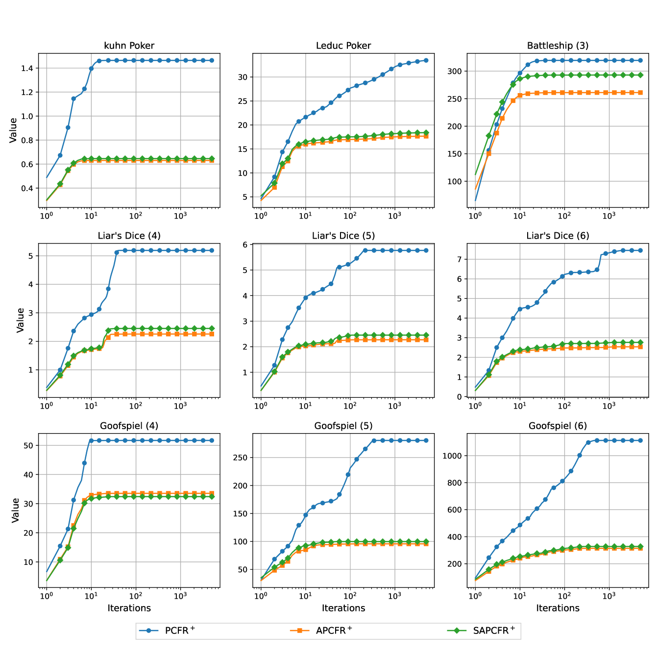
Figure 10: Dynamics of ${\sum^{T}_{t=1}(\frac{\|{\bm{r}}^{t}_{I}-{\bm{r}}^{t-1}_{I}\|^{2}_{2}}{1+\alpha^{t}_{I}}+\alpha^{t}_{I}\|{\bm{R}}^{t+1}_{I}-{\bm{R}}^{t}_{I}\|^{2}_{2})}$ in standard commonly used IIG benchmarks.

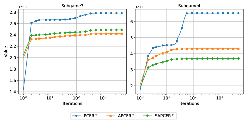
Figure 11: Dynamics of ${\sum^{T}_{t=1}(\frac{\|{\bm{r}}^{t}_{I}-{\bm{r}}^{t-1}_{I}\|^{2}_{2}}{1+\alpha^{t}_{I}}+\alpha^{t}_{I}\|{\bm{R}}^{t+1}_{I}-{\bm{R}}^{t}_{I}\|^{2}_{2})}$ in HUNL Subgames.

Figure 12: Dynamics of ${\sum^{T}_{t=1}\|{\bm{r}}^{t}_{I}-\frac{{\bm{r}}^{t-1}_{I}}{{1+\alpha^{t}_{I}}}\|^{2}_{2}}$ in standard commonly used IIG benchmarks.

Figure 13: Dynamics of ${\sum^{T}_{t=1}\|{\bm{r}}^{t}_{I}-\frac{{\bm{r}}^{t-1}_{I}}{{1+\alpha^{t}_{I}}}\|^{2}_{2}}$ in HUNL Subgames.

References

- Bowling et al. (2015) Bowling, M., Burch, N., Johanson, M., and Tammelin, O. Heads-up limit hold’em poker is solved. Science, 347(6218):145–149, 2015.
- Brown & Sandholm (2018) Brown, N. and Sandholm, T. Superhuman AI for heads-up no-limit poker: Libratus beats top professionals. Science, 359(6374):418–424, 2018.
- Brown & Sandholm (2019a) Brown, N. and Sandholm, T. Solving imperfect-information games via discounted regret minimization. In Proceedings of the 33rd AAAI Conference on Artificial Intelligence, pp. 1829–1836, 2019a.
- Brown & Sandholm (2019b) Brown, N. and Sandholm, T. Superhuman AI for multiplayer poker. Science, 365(6456):885–890, 2019b.
- Chen et al. (2017) Chen, X., Han, Z., Zhang, H., Xue, G., Xiao, Y., and Bennis, M. Wireless resource scheduling in virtualized radio access networks using stochastic learning. IEEE Transactions on Mobile Computing, 17(4):961–974, 2017.
- Farina et al. (2019) Farina, G., Kroer, C., and Sandholm, T. Online convex optimization for sequential decision processes and extensive-form games. In Proceedings of the 33rd AAAI Conference on Artificial Intelligence, pp. 1917–1925, 2019.
- Farina et al. (2021) Farina, G., Kroer, C., and Sandholm, T. Faster game solving via predictive blackwell approachability: Connecting regret matching and mirror descent. In Proceedings of the 35th AAAI Conference on Artificial Intelligence, pp. 5363–5371, 2021.
- Farina et al. (2023) Farina, G., Grand-Clément, J., Kroer, C., Lee, C.-W., and Luo, H. Regret matching+:(in) stability and fast convergence in games. arXiv preprint arXiv:2305.14709, 2023.
- Gordon (2006) Gordon, G. J. No-regret algorithms for online convex programs. In Proceedings of the 19th International Conference on Neural Information Processing Systems, pp. 489–496. MIT Press, 2006.
- Hart & Mas-Colell (2000) Hart, S. and Mas-Colell, A. A simple adaptive procedure leading to correlated equilibrium. Econometrica, 68(5):1127–1150, 2000.
- Hazan et al. (2016) Hazan, E. et al. Introduction to online convex optimization. Foundations and Trends® in Optimization, 2(3-4):157–325, 2016.
- Joulani et al. (2017) Joulani, P., György, A., and Szepesvári, C. A modular analysis of adaptive (non-)convex optimization: Optimism, composite objectives, variance reduction, and variational bounds. In Proceedings of the 30th International Conference on Algorithmic Learning Theory, pp. 681–720, 2017.
- Lanctot et al. (2009) Lanctot, M., Waugh, K., Zinkevich, M., and Bowling, M. Monte carlo sampling for regret minimization in extensive games. In Proceedings of the 22nd International Conference on Neural Information Processing Systems, pp. 1078–1086, 2009.
- Lanctot et al. (2019) Lanctot, M., Lockhart, E., Lespiau, J.-B., Zambaldi, V., Upadhyay, S., Pérolat, J., Srinivasan, S., Timbers, F., Tuyls, K., Omidshafiei, S., et al. Openspiel: A framework for reinforcement learning in games. 2019.
- Langley (2000) Langley, P. Crafting papers on machine learning. In Langley, P. (ed.), Proceedings of the 17th International Conference on Machine Learning (ICML 2000), pp. 1207–1216, Stanford, CA, 2000. Morgan Kaufmann.
- Lisỳ et al. (2016) Lisỳ, V., Davis, T., and Bowling, M. Counterfactual regret minimization in sequential security games. In Proceedings of the 30th AAAI Conference on Artificial Intelligence, pp. 544–550, 2016.
- Liu et al. (2023) Liu, M., Ozdaglar, A. E., Yu, T., and Zhang, K. The power of regularization in solving extensive-form games. In Proceedings of the 12th International Conference on Learning Representations, 2023.
- Liu et al. (2024) Liu, M., Farina, G., and Ozdaglar, A. LiteEFG: An efficient python library for solving extensive-form games. arXiv preprint arXiv:2407.20351, 2024.
- Liu et al. (2021) Liu, W., Jiang, H., Li, B., and Li, H. Equivalence analysis between counterfactual regret minimization and online mirror descent. arXiv preprint arXiv:2110.04961, 2021.
- Meng et al. (2023) Meng, L., Ge, Z., Li, W., An, B., and Gao, Y. Efficient last-iterate convergence algorithms in solving games. arXiv preprint arXiv:2308.11256, 2023.
- Moravč´ık et al. (2017) Moravčík, M., Schmid, M., Burch, N., Lisỳ, V., Morrill, D., Bard, N., Davis, T., Waugh, K., Johanson, M., and Bowling, M. Deepstack: Expert-level artificial intelligence in heads-up no-limit poker. Science, 356(6337):508–513, 2017.
- Nemirovskij & Yudin (1983) Nemirovskij, A. S. and Yudin, D. B. Problem complexity and method efficiency in optimization. 1983.
- Osborne et al. (2004) Osborne, M. J. et al. An introduction to game theory, volume 3. Oxford university press New York, 2004.
- Pérolat et al. (2021) Pérolat, J., Munos, R., Lespiau, J., Omidshafiei, S., Rowland, M., Ortega, P. A., Burch, N., Anthony, T. W., Balduzzi, D., Vylder, B. D., Piliouras, G., Lanctot, M., and Tuyls, K. From Poincaré recurrence to convergence in imperfect information games: Finding equilibrium via regularization. In Proceedings of the 38th International Conference on Machine Learning, pp. 8525–8535, 2021.
- Pérolat et al. (2022) Pérolat, J., De Vylder, B., Hennes, D., Tarassov, E., Strub, F., de Boer, V., Muller, P., Connor, J. T., Burch, N., Anthony, T., et al. Mastering the game of Stratego with model-free multiagent reinforcement learning. Science, 378(6623):990–996, 2022.
- Rakhlin & Sridharan (2013a) Rakhlin, A. and Sridharan, K. Online learning with predictable sequences. In Proceedings of the 26th Annual Conference on Learning Theory, pp. 993–1019, 2013a.
- Rakhlin & Sridharan (2013b) Rakhlin, A. and Sridharan, K. Optimization, learning, and games with predictable sequences. In Proceedings of the 26th International Conference on Neural Information Processing Systems, pp. 3066–3074, 2013b.
- Sandholm (2015) Sandholm, T. Steering evolution strategically: Computational game theory and opponent exploitation for treatment planning, drug design, and synthetic biology. In Proceedings of the 29th AAAI Conference on Artificial Intelligence, pp. 4057–4061, 2015.
- Steinberger (2019) Steinberger, E. Pokerrl. https://github.com/TinkeringCode/PokerRL, 2019.
- Tammelin (2014) Tammelin, O. Solving large imperfect information games using cfr+. arXiv preprint arXiv:1407.5042, 2014.
- Wei et al. (2021) Wei, C., Lee, C., Zhang, M., and Luo, H. Linear last-iterate convergence in constrained saddle-point optimization. In Proceedings of the 9th International Conference on Learning Representations, 2021.
- Xu et al. (2022) Xu, H., Li, K., Fu, H., Fu, Q., and Xing, J. Autocfr: learning to design counterfactual regret minimization algorithms. In Proceedings of the AAAI Conference on Artificial Intelligence, volume 36, pp. 5244–5251, 2022.
- Xu et al. (2024a) Xu, H., Li, K., Fu, H., Fu, Q., Xing, J., and Cheng, J. Dynamic discounted counterfactual regret minimization. In Proceedings of the 12th International Conference on Learning Representations, 2024a.
- Xu et al. (2024b) Xu, H., Li, K., Liu, B., Fu, H., Fu, Q., Xing, J., and Cheng, J. Minimizing weighted counterfactual regret with optimistic online mirror descent. arXiv preprint arXiv:2404.13891, 2024b.
- Zhang et al. (2024) Zhang, N., McAleer, S., and Sandholm, T. Faster game solving via hyperparameter schedules. arXiv preprint arXiv:2404.09097, 2024.
- Zinkevich et al. (2007) Zinkevich, M., Johanson, M., Bowling, M., and Piccione, C. Regret minimization in games with incomplete information. In Proceedings of the 20th International Conference on Neural Information Processing Systems, pp. 1729–1736, 2007.