Quantum critical point followed by Kondo-like behavior due to Cu substitution in itinerant, antiferromagnet ${\text{La}_{2}\text{(Cu}_{x}\text{Ni}_{1-x})_{7}}$

Abstract

$\text{La}_{2}\text{Ni}_{7}$ is an itinerant magnetic system with a small saturated moment of $\sim$ 0.1 $\mu_{B}/\text{Ni}$ and a series of antiferromagnetic (AFM) transitions at $T_{1}$ = 61.0 K, $T_{2}$ = 56.5 K and $T_{3}$ = 42.2 K. $M(H)$, and $\rho(H)$ isotherms as well as constant field $M(T)$ and $\rho(T)$ measurements on single crystalline samples manifest a complex, anisotropic $H-T$ phase diagram with multiple phase lines. Here we present the growth and characterization of single crystals of the ${\text{La}_{2}\text{(Cu}_{x}\text{Ni}_{1-x})_{7}}$ series for 0 $\leq x\leq$ 0.181. We measured powder x-ray diffraction, and composition, as well as anisotropic temperature and field dependent resistivity, temperature and field dependent magnetization and temperature dependent heat capacity on these single crystals. Using the measured data we infer a transition temperature-composition $(T-x)$ phase diagram for this system to study the evolution of the three AFM transitions upon Cu substitution. For ${0\leq x\leq 0.097}$, the system remains magnetically ordered at base temperature with $x\leq$ 0.012, showing signs of three primarily AFM phases. For the higher substitution levels, ${0.125\leq x\leq 0.181}$, there are no signatures of magnetic ordering, but an anomalous feature in resistance and heat capacity data are observed which are consistent with the Kondo effect in this system. The intermediate $x$ = 0.105 sample lies in between the magnetic ordered and the Kondo regime and is in the vicinity of the AFM-quantum critical point (QCP). Thus, ${\text{La}_{2}\text{(Cu}_{x}\text{Ni}_{1-x})_{7}}$ is an example of a small moment system that can be tuned through a QCP. Given these data combined with the fact that the $\text{La}_{2}\text{Ni}_{7}$ structure has kagome-like, Ni-sublattice running perpendicular to the crystallographic $c-$ axis, and a $3d$-electron flat band that contributes to the density of states near the Fermi energy, it becomes a promising candidate to host and study exotic physics.

I Introduction

Itinerant, metallic, magnetic systems with low transition temperatures are often explored in the condensed matter community, as their ordering temperatures can be suppressed by application of pressure, changing the chemical composition (doping), or by magnetic field [1]. Suppressing second-order phase transitions to zero temperature is associated with the emergence of several exotic physical phenomena, such as unconventional superconductivity, non Fermi liquid, etc. are found in proximity of the quantum critical point (QCP) [1, 2, 3, 4, 5, 6, 7, 8, 9, 10, 11, 12, 13]. Intensive studies have shown that although antiferromagnetic (AFM) transitions in many metallic systems can be continuously suppressed to zero temperature by the non-thermal tuning parameters discussed above [1, 14, 8, 15, 16, 17], the situation becomes quite different for ferromagnetic (FM) transitions. The current theoretical as well as experimental studies suggest that stoichiometric systems with minimum disorder generally avoid a FM quantum critical point (QCP) at zero field [2, 18, 19, 20]. Although, for AFM systems, hydrostatic pressure, and applied magnetic field are the preferred choices for suppression of transition temperature, the reason being that they do not introduce any additional disorder, chemical substitution, despite inducing a degree of disorder, is another, often more versatile, tuning parameter to access QCP and, more generally, tune the ground state in these systems.

$\text{La}_{2}\text{Ni}_{7}$, which belongs to the $\text{Ce}_{2}\text{Ni}_{7}$ (space group P6/mmm, #194) family, had been suspected to be a small moment antiferromagnet for decades, but prior studies on polycrystalline samples left the nature and even the number of its low temperature states unclear [21, 22, 23, 24, 25, 26, 27, 28, 29]. Recently large, well-faceted, hexagonal single crystalline plates of $\text{La}_{2}\text{Ni}_{7}$ were synthesized, and anisotropic transport, magnetization, and heat capacity measurements done on these crystals revealed a series of antiferromagnetic (AFM) transitions at $T_{1}$ = 61.0 K, $T_{2}$ = 56.5 K and $T_{3}$ = 42.2 K [30]. With a saturated moment of $\sim$ 0.1 $\mu_{B}/\text{Ni}$ and an effective moment of $\sim$ 1.0 $\mu_{B}/\text{Ni}$, $\text{La}_{2}\text{Ni}_{7}$, clearly is a small moment itinerant magnetic system. The anisotropic $H-T$ phase diagram constructed identified multiple magnetic regions. These findings were further confirmed by single crystal neutron diffraction [31], ARPES [32] and NMR/NQR [33] measurements on this system.

Whereas an initial study of $\text{La}_{2}\text{Ni}_{7}$ under hydrostatic pressure found the three transitions to be only weakly changed up to 2 GPa [30], the small itinerant moment found in this system may suggest close proximity to a QCP and still make this material an attractive candidate for further investigations. In particular, Fig. 1 shows that the $Ni4$ and $Ni5$ atoms, occupying respectively the Wyckoff positions 12k and 6h, [22] in $\text{La}_{2}\text{Ni}_{7}$ form Kagome-like networks. In such structures, destructive interference associated with frustrated electron hoping pathways is predicted to support flat bands, if they are close enough to the Fermi level, that may be related to magnetic (or other ) instabilities. Indeed, density functional theory (DFT) calculations predicted a flat, $Ni-3d$ band near $E_{F}$ [32]. Given that ARPES measurements did not detect this band [32], it is speculated that this flat band may be slightly above $E_{F}$, and may be accessible with electron doping.

In this paper, we report the synthesis and physical properties of electron doped ${\text{La}_{2}\text{(Cu}_{x}\text{Ni}_{1-x})_{7}}$ with ${0\leq x\leq 0.181}$. Single crystals of ${\text{La}_{2}\text{(Cu}_{x}\text{Ni}_{1-x})_{7}}$ were grown and their temperature and field dependent magnetization, temperature dependent resistivity, and temperature dependent heat capacity were investigated. Our studies reveal that for ${0\leq x\leq 0.097}$, the system remains magnetically ordered at base temperature with the low dopings $x\leq$ 0.012 showing signs of three AFM phases. The temperature of the highest transition decreases monotonically, and magnetic order is suppressed below $T$ = 1.8 K for $x>$ 0.097. The samples with higher substitution levels, ${0.125\leq x\leq 0.181}$, manifest no signatures of magnetic ordering and instead have a low temperature upturn in $\rho(T)$ and $C_{p}/T$, which are features that are associated with Kondo-like behavior. The intermediate substitution $x$ = 0.105 lies in between the magnetic ordered and the Kondo regime, shows behavior characteristic of a non-Fermi liquid (nFL) in the resistivity data, and is in the vicinity of the QCP for this system.

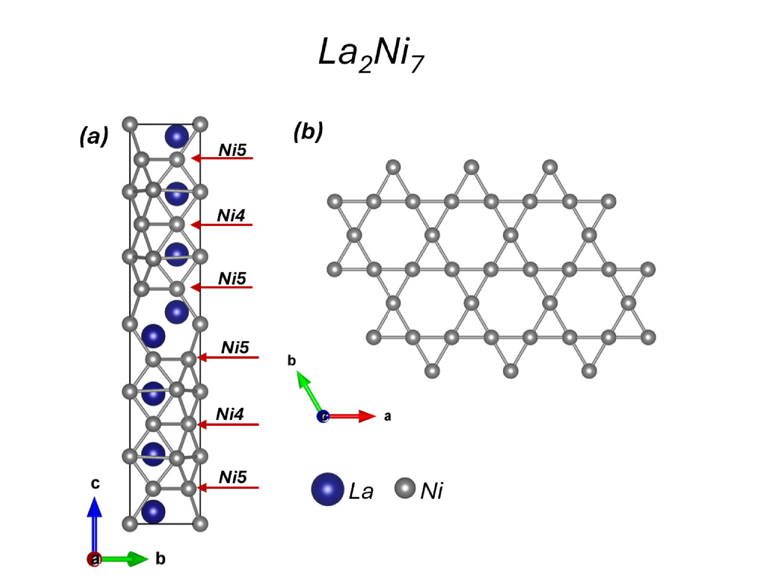
Figure 1: (Color online) (a) The crystal structure of $\text{La}_{2}\text{Ni}_{7}$ as generated by VESTA [34]. The Ni4 and Ni5 planes are equivalent and have been marked by red arrows. (b) The Ni4/Ni5 plane along the $ab-$ plane which form a kagome lattice.

II Experimental Methods

Single crystals of ${\text{La}_{2}\text{(Cu}_{x}\text{Ni}_{1-x})_{7}}$; with ${x_{nominal}}$ = 0, 0.01, 0.015, 0.02, 0.03, 0.05, 0.07, 0.09, 0.10, 0.12, 0.15, and 0.18 were synthesized using a self flux, solution growth method [35, 36, 37] in a manner similar to the growth of pure $\text{La}_{2}\text{Ni}_{7}$ [30]. Small pieces of lanthanum (Materials Preparation Center - Ames National Laboratory $99.99\%$), nickel (Alfa Aesar $99.98\%$), and copper (Ames National Laboratory $99.99\%$) with a starting composition of ${\text{La}_{33}\text{(Cu}_{x}\text{Ni}_{1-x})_{67}}$, were weighed, then placed into a tantalum, 3-cap-crucible [35, 36], and sealed in a fused silica ampoule under a partial argon atmosphere. The ampoule was heated in a box-furnace to $1180\tccentigrade$ over 10 hours, held at the temperature for 20 hours to ensure a homogeneous melt, quickly cooled down to $1020\tccentigrade$ followed by a very slow cool to $820\tccentigrade$ over 200 hours. After dwelling at $820\tccentigrade$ for a few hours, the excess solution was then decanted using a centrifuge [37, 36, 35]. Well-faceted hexagonal plates of single crystalline ${\text{La}_{2}\text{(Cu}_{x}\text{Ni}_{1-x})_{7}}$ were obtained having typical dimensions of ${\sim 4~\text{mm}\times\sim 4~\text{mm}}$ with an average thickness of ${\sim 1~\text{mm}}$ and of the same morphology as that of the undoped compound. (See the inset to Fig 2(a), or inset to Fig 1 in Ref [30] for pictures of representative crystals). Increasing the $x_{nominal}~\geq$ 0.20 in the ${\text{La}_{33}\text{(Cu}_{x}\text{Ni}_{1-x})_{67}}$ melt yielded single crystals of ${\text{La}\text{(Cu}_{x}\text{Ni}_{1-x})_{5}}$, with $x\sim 0.3$ and hence we stopped the attempts of substitution at ${x_{nominal}}$ = 0.18.

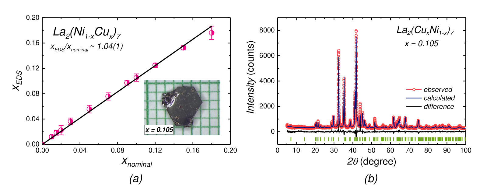
Figure 2: (a) Measured Cu substitution level, ($x_{EDS}$) values, for ${\text{La}_{2}\text{(Cu}_{x}\text{Ni}_{1-x})_{7}}$ crystals versus $x_{nominal}$ values used in the growth solution. The black line corresponds to the linear fit across the data points with the intercept fixed to (0,0), and a slope of essentially 1, clearly showing that $x_{EDS}$ $\sim$ with $x_{nominal}$. (Inset: typical crystals of ${\text{La}_{2}\text{(Cu}_{x}\text{Ni}_{1-x})_{7}}$ for $x_{EDS}$ = 0.105 on a mm grid.) (b) Powder X-Ray diffraction data for ${\text{La}_{2}\text{(Cu}_{x}\text{Ni}_{1-x})_{7}}$ for $x_{EDS}=0.105$. The data for other $x$-values are qualitatively the same.

The Cu substitution levels $x_{EDS}$ of the ${\text{La}_{2}\text{(Cu}_{x}\text{Ni}_{1-x})_{7}}$ crystals were determined by Energy Dispersive Spectroscopy (EDS) quantitative chemical analysis. All SEM images were acquired with the ThermoFisher (FEI) Teneo Lovac FE-SEM, located at the Sensitive Instrument Facility, Ames National Laboratory. The data was analyzed using an Oxford Instruments Aztec System with a X-Max-80 detector, attached to the Teneo. An acceleration voltage of 15 kV, current of 1.6 nA, working distance of 10mm and take off angle of 35${\degree}$ were used for measurements. The composition of the crystals was measured at 7-8 different spots on the crystal’s face, revealing good homogeneity of each crystal except for the highest doped sample ($x_{nominal}$ = 0.18). The standards used for reference are internal to the Oxford software.

The phase and crystal structure was confirmed using a Rigaku Miniflex-II powder diffractometer using Cu ${K_{{\alpha}}}$ radiation $(\lambda=1.5406~$\mathrm{\text{Å}}$)$. Single crystals were finely ground, and the powder was then mounted and measured on a single crystal Si, zero-background sample holder using a small amount of vacuum grease. Intensities were collected for 2$\theta$ ranging from $5\degree$ to $100\degree$ in steps of $0.01\degree$, counting each angle for 5 seconds. The patterns were refined and the lattice parameters were determined using GSAS II software. [38].

Temperature $(M(T))$ and field $(M(H))$ dependent DC magnetization measurements were made in a Quantum Design Magnetic Property Measurement System (QD-MPMS classic) SQUID magnetometer with samples mounted on a diamagnetic Poly-Chloro-Tri-Fluoro-Ethylene (PCTFE) disk, which snugly fits inside a straw, using a small amount of superglue. Each sample was measured with the external field applied parallel ($H||c$) and perpendicular ($H\perp c$) to the hexagonal $c$ - axis as was done for the parent compound [30]. Additionally, Curie-Weiss analysis was done on the magnetic susceptibility ($\chi=M(T)/H)$ data for $H||c$ and $H\perp c$ data as well as for a polycrystalline average of these data sets. The polycrystalline average susceptibility of the hexagonal samples was obtained by using $\chi_{poly}=\frac{1}{3}\chi_{||c}+\frac{2}{3}\chi_{\perp c}$ where $\chi_{||c}$ and $\chi_{\perp c}$ are the magnetic susceptibilities along $H||c$ and $H\perp c$ respectively. The signal from the disk was measured beforehand and subtracted from the combined sample-disk magnetization data for both directions so as to obtain the value of the moment due to the sample for each $H||c$ and $H\perp c$. Both $M(H)$ and $M(T)$ measurements were done under zero-field cooled (ZFC) protocol where the sample was cooled down to 1.8 K before applying the external magnetic field. In some additional cases field-cooled (FC) protocol was also employed when the samples were cooled down in presence of the externally applied field. $M(H)$ measurements were done in magnetic fields from 0 kOe to 70 kOe whereas $M(T)$ measurements were done in the temperature range between 1.8 K and 300 K.

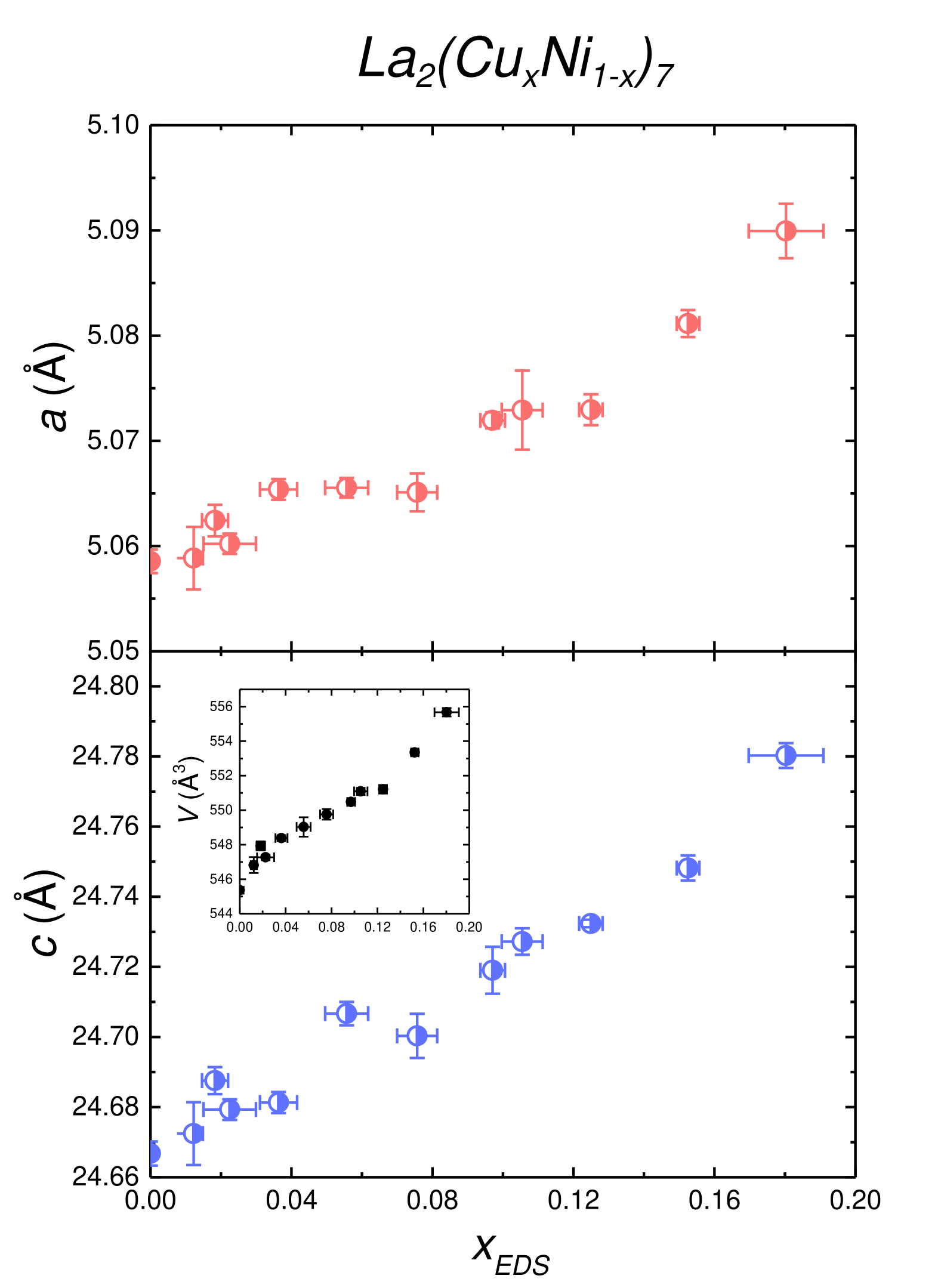
Figure 3: Lattice parameters $a-$ on the top panel, and $c-$ on the bottom panel and the unit cell volume, $V$ (as an inset in the bottom panel) as a function of the Cu substitution level $(x_{EDS})$ in ${\text{La}_{2}\text{(Cu}_{x}\text{Ni}_{1-x})_{7}}$ single crystals obtained from the refinement of the powder x-ray diffraction data.

Temperature dependent ac resistivity measurements $(\rho(T))$ were done in the standard four-probe geometry in a Quantum Design Physical Property Measurement System (QD-PPMS) using a 3 mA excitation with a frequency of 17 Hz in the $ab$ plane of the crystals. $\rho(T)$ was measured with the current flowing in the basal plane (i.e. perpendicular to the c-axis). The hexagonal plate like samples of each $x$ of ${\text{La}_{2}\text{(Cu}_{x}\text{Ni}_{1-x})_{7}}$ were cut into bars with a wire saw and had dimensions of roughly 2 mm long, 0.8 mm wide, and 0.2 mm thick (along the c direcion). Electrical contacts were made using 25 $\mu m$ diameter platinum wires attached to the bar shaped samples using Epotek-H20E epoxy. $\rho(T)$ was measured in the range of $1.8~\text{K}\leq T\leq 300~\text{K}$ under zero magnetic field and in some cases under a magnetic field (both $H\perp c$ and $H||c$ directions).

Temperature dependent heat capacity measurements were performed in a QD-PPMS. Plate-like samples were mounted on the micro-calorimeter platform using a small amount of Apeizon N-grease and measured under zero magnetic field. The addenda (contribution from the grease and the sample platform) was measured separately and subtracted from the total data to obtain the contribution only due to the sample using the PPMS software.

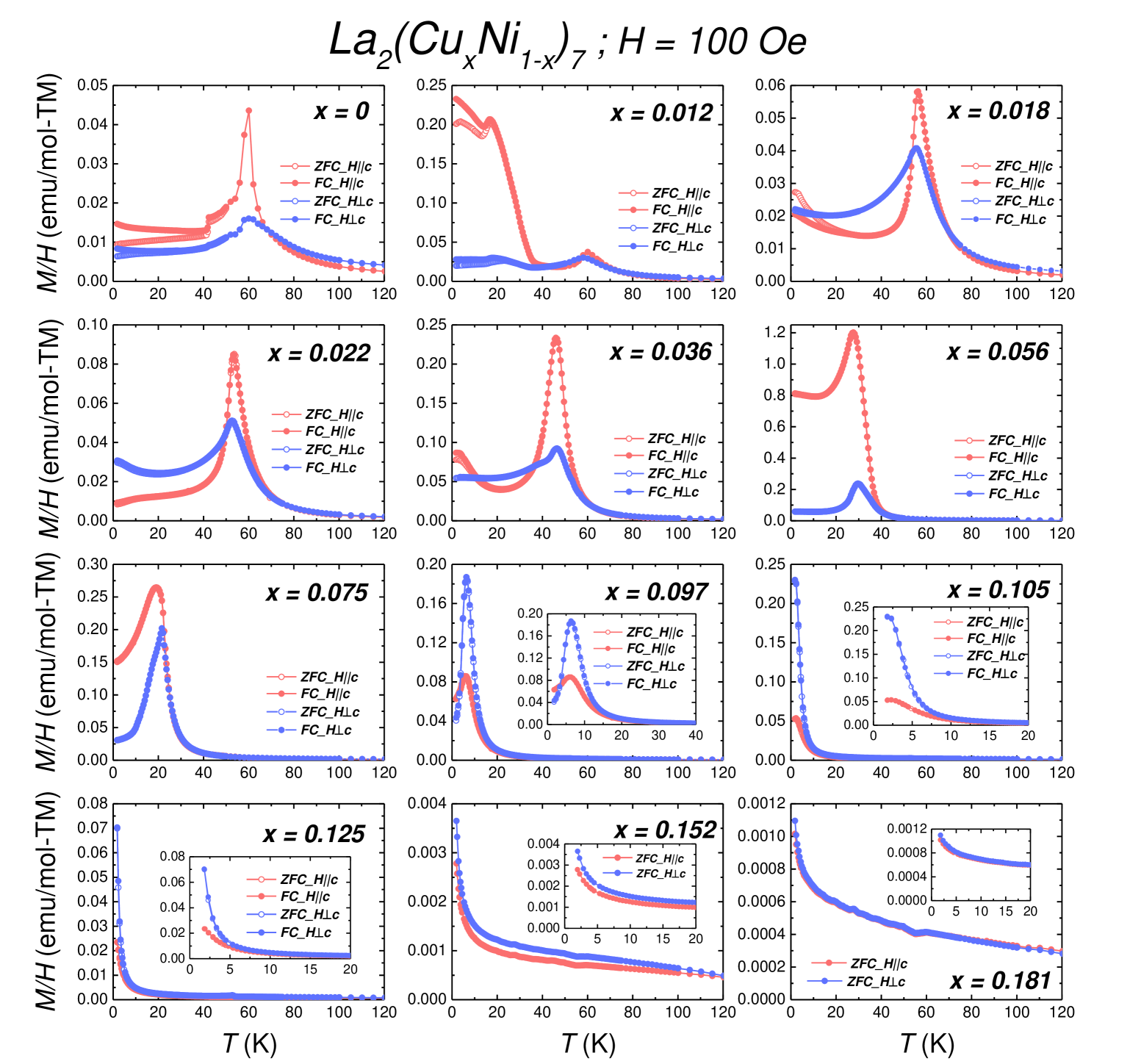
Figure 4: (Color online) Anisotropic temperature dependent magnetization ($M(T)$) measured at $H$ = 100 Oe for ${\text{La}_{2}\text{(Cu}_{x}\text{Ni}_{1-x})_{7}}$ single crystals. $M(T)$ for each Cu substituted sample is plotted in separate panels for both $H||c$ and $H\perp c$. Although measurements were done up to $T=300$ K, the data here is plotted only until T$=120$ K to highlight the transition related features. The samples were measured for both ZFC-FC mode for 0 $\leq x\leq$ 0.125 and only in ZFC mode for $x$ = 0.152 and 0.181. Some of the panels (0.097 $\leq x\leq$ 0.181) have insets to show the low temperature behavior in greater detail.

III Results

Composition and lattice parameters

The Cu substitution levels in ${\text{La}_{2}\text{(Cu}_{x}\text{Ni}_{1-x})_{7}}$ single crystals, determined by the EDS measurements $(x_{EDS})$ are plotted as a function of the nominal Cu levels $(x_{nominal})$, used for the growths are shown in Fig 2(a). As $x_{nominal}$ is increased, $x_{EDS}$ increases in a monotonic and almost linear manner. The best fit line, going through the $(x_{EDS})$ data has a slope of 1.04(1), and can be seen as operationally indistinguishable from 1.0. From this point onwards, in this paper, $x$ will refer to the Cu substitution values determined by EDS measurements in ${\text{La}_{2}\text{(Cu}_{x}\text{Ni}_{1-x})_{7}}$. In the rare case when we need to refer to the nominal Cu concentration in the growth melt we will explicitly use the $x_{nominal}$ notation.

Figure 2(b) shows a representative powder x-ray diffraction pattern for ${\text{La}_{2}\text{(Cu}_{x}\text{Ni}_{1-x})_{7}}$ for the $x=0.105$ sample. Similar x-ray patterns for crystals of each Cu substitution were refined and the lattice parameters $a=b$, and $c$ as well as the unit cell volume $V$ were obtained after refinement of the powder diffraction data. The peaks are matched with the expected peaks of the ${\text{Ce}_{2}\text{Ni}_{7}}$ hexagonal structure with space group $P6_{3}/mmc$, (No. 194) structure type [22]. Fig 3 shows the change in the lattice parameters $a$, $c$, and the unit cell volume $V$ of ${\text{La}_{2}\text{(Cu}_{x}\text{Ni}_{1-x})_{7}}$ versus $x$. There is an increase in $a$, $c$, and $V$ as we increase the Cu substitution level. Given that the difference in ionic radii between Ni and Cu is small and the substitution level is less than $x$ = 0.20, it is not surprising that the changes in the lattice parameters and volume are small, albeit clearly resolvable. The values of the lattice parameters for each of the $x$ values are shown in Table 1 in the Appendix.

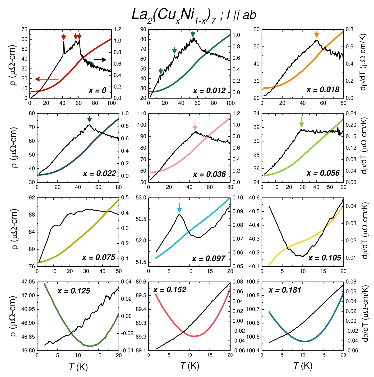
Figure 5: Temperature dependent, zero field in-plane resistivity on the left axis and its corresponding derivative on the right axis of ${\text{La}_{2}\text{(Cu}_{x}\text{Ni}_{1-x})_{7}}$ single crystals plotted in separate panels. The colored curves show the $\rho(T)$ data and the black curves the corresponding $\frac{d\rho}{dT}$. $\rho(T)$ for $0\leq x\leq 0.097$ are plotted starting above their respective magnetic ordering temperatures down to 1.8 K whereas for the higher doped samples, $0.105\leq x\leq 0.181$, which do not show magnetic ordering, resistivity is plotted from 20 K down to 1.8 K. The magnetic ordering temperatures determined from maxima in the derivative data are shown in each panel using arrows.

Zero and low-field data and $T-x$ phase diagram

Low field $M(T)$

Figure 4 shows the anisotropic $M(T)$ data measured at 100 Oe for both $H||c$ and $H\perp c$ for each Cu substituted sample and is shown. For 0 $\leq x\leq$ 0.125, the data was measured in both ZFC-FC protocols, whereas for the two highest dopings $x$ = 0.152 and 0.181 the data was measured only in ZFC mode. For the parent compound ($x$ = 0) as well as for the lowest doped sample ($x$ = 0.012), we observe signs of three magnetic transitions. Increasing the Cu substitution level suppresses the transitions, so that when $x$ reaches 0.018, only the highest temperature transition remains. This transition is further suppressed with Cu substitution, but is observable up to $x$ = 0.097. We also observe a distinct ZFC-FC split for 0 $\leq x\leq$ 0.036, but not for the higher $x$ samples which show magnetic order down to $T$ = 1.8 K (0.056 $\leq x\leq$ 0.097). This may imply that the magnetic state associated with one of the two lower transitions, has a small but finite FM component. This will be further discussed in the Appendix.

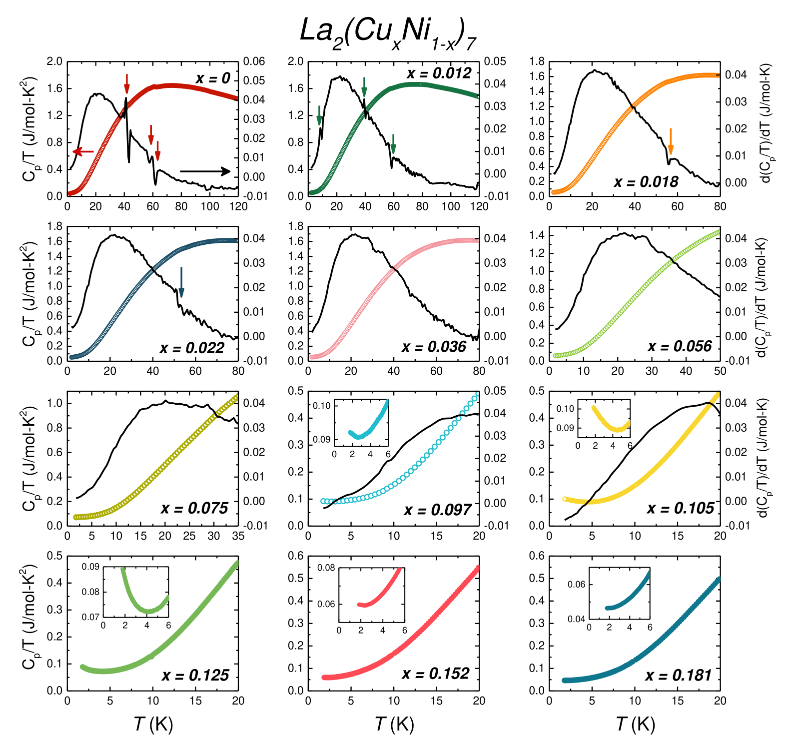
Figure 6: (Color online) Temperature dependent, zero field, $C_{p}/T$ data of the ${\text{La}_{2}\text{(Cu}_{x}\text{Ni}_{1-x})_{7}}$ single crystals on the left axis (colored curves) and its corresponding derivative plotted on the right axis (black curves) in separate panels for each concentration. The derivatives are not plotted for the three highest dopings, 0.125 $\leq x\leq$ 0.181, as there are no distinct features related to any transition. The magnetic ordering feature(s) is visible in the derivative for 0 $\leq x\leq$ 0.022 and is shown using arrows. $x$ = 0.036 and 0.056 samples have broader features in their derivatives which may be related to the transition but are not clearly resolvable. For 0 $\leq x\leq$ 0.097, the data is plotted from temperatures above their magnetic transition down to 1.8 K. For 0.105 $\leq x\leq$ 0.181, the data are plotted from 20 K down to the base temperature. The data set for the parent $x=0$ is from Ref [30]. For $x\geq$ 0.097, the plots have insets which show the low temperature behavior of the data.

For $x$ = 0.105, no feature associated with a transition is observed down to 1.8 K. Finally, for the highest doped samples, $0.125\leq x\leq 0.181$, we observe a $M(T)$ behavior characteristic of a paramagnet. Thus, the antiferromagnetic long range magnetic ordering in ${\text{La}_{2}\text{(Cu}_{x}\text{Ni}_{1-x})_{7}}$ is suppressed below the base temperature, or, completely, due to Cu substitution for $x>0.097$.

In order to more quantitatively parametrize the number and location of ordering temperatures we plot the polycrystalline average $\frac{d\chi T}{dT}$ for the $x\leq 0.097$ samples shown in Fig 17 in the Appendix. The magnetic transition temperatures inferred are plotted in the $T-x$ phase diagram in Fig 7 below.

$\rho(T)$ in zero applied magnetic field

Figure 5 shows the temperature dependent in-plane ($I||ab-$ plane) resistivity of the ${\text{La}_{2}\text{(Cu}_{x}\text{Ni}_{1-x})_{7}}$ single crystals in separate panels. For $0\leq x\leq 0.097$, the data is plotted over temperature ranges that highlight the magnetic ordering transitions, with a base temperature of 1.8 K. For the 0 $\leq x\leq$ 0.097 samples, we observe metallic behavior for temperatures above the magnetic ordering and for $0.105\leq x\leq 0.181$, metallic behavior is observed for $T\geq 15$ K . The residual resistance ratio $(RRR=\rho(300~\text{K})/\rho(1.8~\text{K}))$ decreases abruptly from $\sim$ 19 for $x=0$ to $\sim$ 6 for $x=0.012$ and then slowly decreases to attain a value of 1.8 for $x=0.105$.

The resistivity of the ${\text{La}_{2}\text{(Cu}_{x}\text{Ni}_{1-x})_{7}}$ single crystals changes its behavior with Cu substitution, especially the higher doped samples. For $0\leq x\leq 0.097$, a modest, but clear loss of spin-disorder scattering is seen in the $\rho(T)$ data upon cooling, indicating the onset of magnetic ordering, with the associated feature more evident for the low dopings ($0\leq x\leq 0.036$). This is also evident from the $\frac{d\rho}{dT}$ data that are shown along the right hand axis using black curve in Fig 5 and Fig 17 in the Appendix.

The resistivity for the highest doped ${\text{La}_{2}\text{(Cu}_{x}\text{Ni}_{1-x})_{7}}$ samples, $0.125\leq x\leq 0.181$, have an entirely different low temperature, behavior and exhibits a minimum at around $T\sim$ 12 K, such that $\rho(T)$ decreases and then further increases as the samples are cooled down to $T$ = 1.8 K. The $x$ = 0.105 sample is intermediate to the higher and lower $x$-samples. As temperature decreases, the $x$ = 0.105 data appears to be going through a resistive minimum, similar to higher $x$-value samples, such that $\rho(T)$ decreases with a linear temperature dependence as base temperature is approached. Further analysis of this sample and its transport data will be given below.

To summarize the results of the resistivity measurements on ${\text{La}_{2}\text{(Cu}_{x}\text{Ni}_{1-x})_{7}}$. (i) We initially see suppression of the magnetic order by observing loss of spin-disorder scattering in the lower doped samples $(0\leq x\leq 0.097)$. (ii) We see a resistive upturn in the highest doped samples $(0.125\leq x\leq 0.181)$, which may be an indication of a Kondo-like behavior in this system and will be discussed in detail in a separate section, below. (iii) The $x$ = 0.105 sample lies at the border of the two regimes with competing interactions and is expected to be in a quantum critical region of the $T-x$ phase diagram (i.e. near the QCP).

Specific Heat in zero applied magnetic field

We measured temperature-dependent heat capacity on the samples to get more insight into the evolution of the transition temperature(s) and the subsequent Kondo like behavior in the ${\text{La}_{2}\text{Ni}_{7}}$ system due to Cu substitution. Figure 6 shows the results of $C_{p}$ measurements on the ${\text{La}_{2}\text{(Cu}_{x}\text{Ni}_{1-x})_{7}}$ single crystals plotted as $C_{p}/T$ vs $T$. The samples were measured over different temperature ranges, depending on their respective magnetic transitions. For each sample, we started at a temperature above their respective highest magnetic transition and measured down to $T$ = 1.8 K. As reported in [30], the three phase transitions for $x$ = 0 are resolvable but the features are quite small. We also plot the corresponding derivatives on the right hand axis to delineate the features due to phase transitions.

For the lower dopings, 0 $\leq x\leq$ 0.022, we observe small features in $C_{p}/T$ and the corresponding derivative at similar temperatures as those of the transitions in the $M(T)$ (Fig 4) and $\rho(T)$ (Fig 5) data, with $x$ = 0 and 0.012 having three distinct features and $x$ = 0.018 and 0.022 only a single feature. For 0.036 $\leq x\leq$ 0.075, despite having magnetic transitions in their $M(T)$ data and clear features in the $\rho(T)$ data, we cannot resolve any associated feature in the specific heat data. Loss of a resolvable specific heat anomaly at the ordering temperature is consistent with the diminishing of an already small ordered moment and the corresponding decrease in the entropy change associated with the transition. The situation becomes different for the highest dopings, $0.097\leq x\leq 0.181$, where the low temperature data shows minima in $C_{p}/T$ at $T\sim$ 5 K, followed by a lower temperature upturn. The upturn increases as we increase the Cu substitution level and is largest (at $T$ = 2 K) for $x$ = 0.105 after which it decreases for the higher dopings, becoming very small, but still resolvable at the highest dopings.

$T-x$ phase diagram

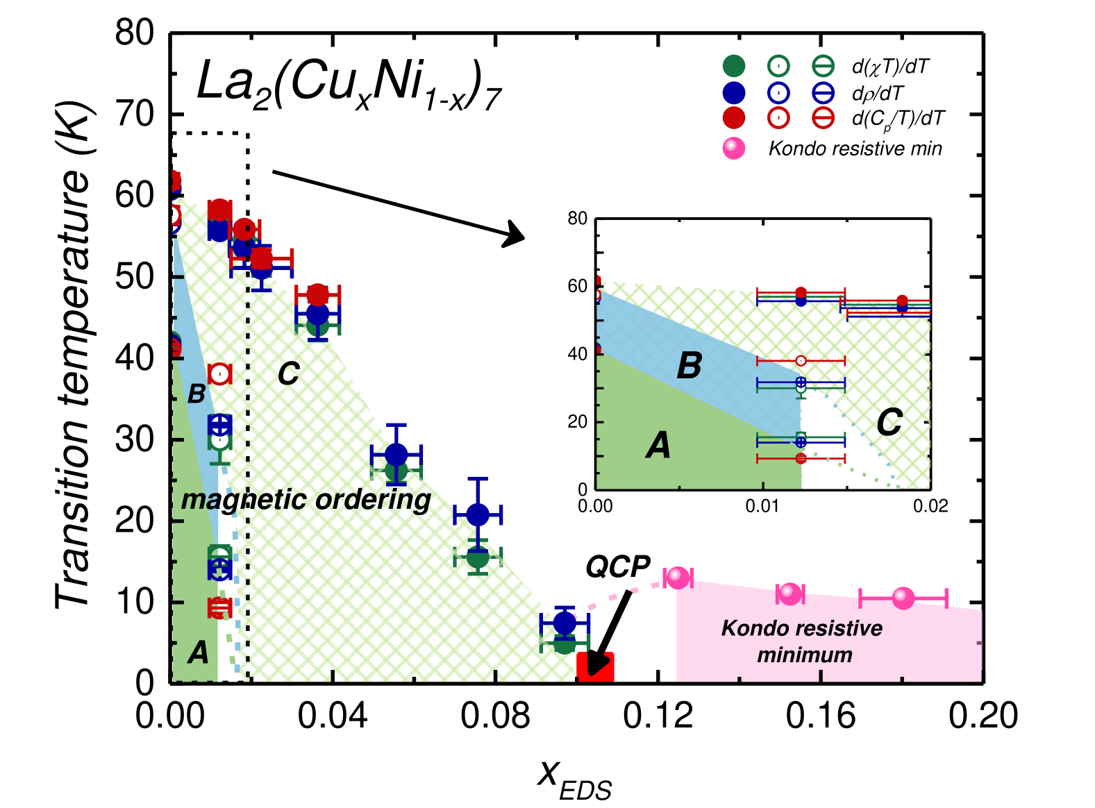
Figure 7: (Color online) The $T-x$ phase diagram for Cu substituted ${\text{La}_{2}\text{(Cu}_{x}\text{Ni}_{1-x})_{7}}$ system constructed from $M(T)$ at 100 Oe and zero field $\rho(T)$ and $C_{p}/T$ data. The 0 $\leq x\leq$ 0.097 regime manifests magnetic order above 1.8 K, with the parent and the lowest doped samples ($x$ = 0 and 0.012) showing signs of three transitions. The three ordered regimes are labeled as $A,B$, and $C$. The inset shows the behavior of the low dopings (0 $\leq x\leq$ 0.02) highlighting the extent of phases $A$ and $B$. The boundary lines for these phases have been extrapolated to T = 0 which may give us an assumption on how $A$ and $B$ might drop to below base temperature between 0.012$\leq x\leq$ 0.018. These phases do not exist for $x\geq$ 0.018. The three higher doped (0.125 $\leq x\leq$ 0.181) samples show a resistive upturn at low temperatures which probably an indicative of some type of Kondo behavior and is shown using the pink area. Like the magnetically ordered regime, the boundary line for the Kondo area has also been extrapolated to T = 0 (with pink dashed lines) towards the low dopings. The intermediate $x$ = 0.105, is in the vicinity of the QCP for this system.

Figure 7 shows the $T-x$ phase diagram of the ${\text{La}_{2}\text{(Cu}_{x}\text{Ni}_{1-x})_{7}}$ series constructed from $M(T)$ measured at 100 Oe and zero field $\rho(T)$ and $C_{p}(T)$ data. The phase diagram can be broadly divided into three distinct regimes. (i) The magnetically ordered lower dopings, 0 $\leq x\leq$ 0.097, (ii) the higher substituted 0.125 $\leq x\leq$ 0.181 regime which show a low $T$ upturn in resistivity and $C_{p}/T$ data, suggesting Kondo-like behavior, and (iii) the intermediate $x\simeq$ 0.105, very close to where the QCP is inferred for this system. We will discuss the behavior of each of these regimes separately.

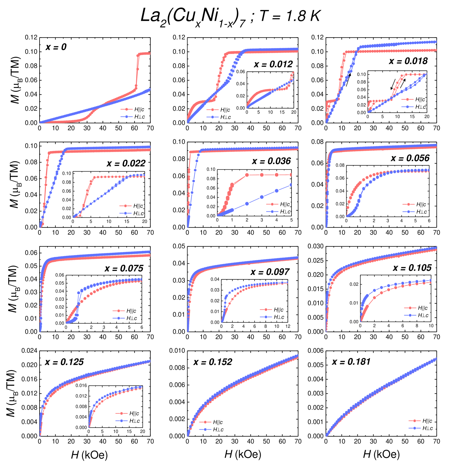
Figure 8: (Color online) Anisotropic field dependent magnetization ($M(H)$) measured at $T$ = 1.8 K for ${\text{La}_{2}\text{(Cu}_{x}\text{Ni}_{1-x})_{7}}$ single crystals. $M(H)$ for each Cu substituted sample is plotted in separate panels for both $H||c$ and $H\perp c$. The samples were cooled down to 1.8 K in the absence of an external field (ZFC) and then measured first for increasing from zero and then followed by decreasing field to zero. Some of the panels ($x$ = 0.012, 0.018, 0.022, 0.036, 0.056, 0.075, 0.097, 0.105, and 0.125) have insets to show the low field behavior in detail.

The magnetic regime is subdivided into three sub-regimes $A$, $B$, and $C$ with only the parent ($x$ = 0) and the lowest doped ($x$ = 0.012) showing all three magnetic phases. The 0.018 $\leq x\leq$ 0.097 region shows only a single magnetic transition. We anticipate that the lower phases drop to below our base temperature between $x$ = 0.012 and 0.018 and indicate this by leaving a blank low temperature region between these substitution levels. From our previous work on the parent $\text{La}_{2}\text{Ni}_{7}$ [30], we expect these phases to be primarily antiferromagnetic with some small ferromagnetic component. The nature of these transitions will be studied in details in the Appendix. As discussed earlier, the polycrystalline $\frac{d(\chi T)}{dT}$, together with $\frac{d(\rho)}{dT}$, and $\frac{dC_{p}/T}{dT}$ data are used to determine the transition temperatures [39, 40]. The position of the local extrema is each of these data determines the value of $T_{N}$. Figures 5 and 6 show the $\frac{d\rho}{dT}$ and the $\frac{dC_{p}/T}{dT}$ plots respectively whereas Fig 17 in the Appendix shows the polycrystalline $\frac{d(\chi T)}{dT}$. The paramagnetic to magnetic transition (phase $C$) decreases monotonically from a value of $\sim$ 60 K for $x$ = 0 [30] to $\sim$ 5 K for $x$ = 0.097. There is good agreement between the $T_{N}$ values inferred from $\chi(T)$, $\rho(T)$, and $C_{p}(T)$ data.

For the three highest Cu dopings, (0.125 $\leq x\leq$ 0.181) where the resistive upturn is observed, the resistive minima is plotted as a proxy for a cross over temperature into the low temperature state. The upturn regime, which maybe due to the Kondo effect, for these substitutions is shown by the pink area in Fig 7. $x$ = 0.105, which is in the vicinity of the QCP for this system is also marked in the phase diagram. The Kondo regime is extrapolated to T = 0 for the low dopings as a possible extension of this low temperature state.

Higher field magnetization measurements

The $T-x$ phase diagram was instrumental in categorizing the global features in the ${\text{La}_{2}\text{(Cu}_{x}\text{Ni}_{1-x})_{7}}$ system. The low dopings (0 $\leq x\leq$ 0.097) have magnetic ordering for temperatures above 1.8 K with $x$ = 0 and 0.012 showing signatures of three magnetic phases. The nature of these magnetic phases can be further illuminated by discussing $M(H)$ data as well as $M(T)$ measured at higher fields.

$M(H)$ at base temperature

Figure 8 shows the anisotropic field dependent magnetization ($M(H)$) measured at $T$ = 1.8 K for ${\text{La}_{2}\text{(Cu}_{x}\text{Ni}_{1-x})_{7}}$ for each Cu substituted sample on separate panels. The $M(T)$ data at 100 Oe (Fig 4) shows that the magnetic state for 0 $\leq x\leq$ 0.097 is primarily antiferromagnetic in nature. The data in Fig 8 also indicates that the base temperature magnetic state in ${\text{La}_{2}\text{(Cu}_{x}\text{Ni}_{1-x})_{7}}$ remains fundamentally antiferromagnetic (AFM) for these Cu substitutions (In the appendix we will discuss what appears to be an exceptionally small FM component to some of these low field states.). We also observe metamagnetic transitions in the data. The metamagnetic transition field $H_{C}$ changes rapidly as we increase the Cu substitution level, as shown in Fig 18 in the Appendix. For $H||c$, the transition field to the saturated paramagnetic state decreases rapidly from $\sim$ 60 kOe to $\sim$ 20 kOe just for $x$ = 0.012 and is completely suppressed by $x$ = 0.036. A lower field transition is observed near 30 kOe for the parent compound which is suppressed even more rapidly with Cu substitution and is no longer observed for $x>0.02$. For $H\perp c$, assuming there is no in-plane anisotropy, the transition to the paramagnetic state is observed and is suppressed more gradually and only dropping below our base temperature at a much higher Cu substitution level of $x$ = 0.097.

Evolution of $\mu_{s}$ and $\mu_{eff}$ with Cu-substitution

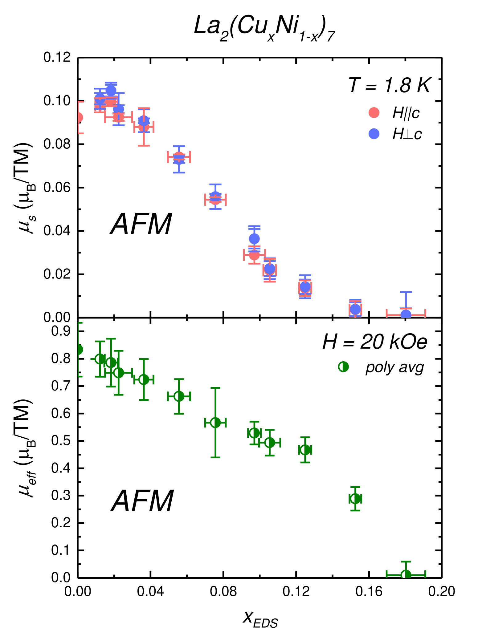
Figure 9: The evolution of the extrapolated moment $\mu_{s}$ and the effective moment $\mu_{eff}$ with $x$ in ${\text{La}_{2}\text{(Cu}_{x}\text{Ni}_{1-x})_{7}}$. The value of $\mu_{s}$ is almost an order of magnitude smaller than the $\mu_{eff}$ confirming the itinerant nature of magnetism in this system.

We can further analyze the change in the magnetic ordering with Cu substitution by studying the change in the high-field, extrapolated moment ($\mu_{s}$) and the effective moment $\mu_{eff}$ obtained from both $M(H)$ and $M(T)$ measurements respectively. Considering, $\mu_{s}$ as a proxy for the saturated moment in an itinerant magnetic system. The top panel of Fig. 9 tracks the evolution of the extrapolated $\mu_{s}$ moment with $x$. $\mu_{s}$ is estimated by extrapolating the high-field (40 kOe $\leq H\leq$ 70 kOe) linear behavior of the $M(H)$ data to zero field as shown in Fig 23 and discussed in details in the Appendix. We see that $\mu_{s}$ decreases as we increase the Cu substitution in ${\text{La}_{2}\text{(Cu}_{x}\text{Ni}_{1-x})_{7}}$ from a value $\sim$ 0.1 $\mu_{B}/TM$ for the parent compound to essentially zero for $x$ = 0.181.

We also track the evolution of the effective moment $\mu_{eff}$ with $x$ from the polycrystalline average of the $\chi(T)$ data by doing a Curie-Weiss analysis with an added temperature independent contribution, fitting the data in the high temperature paramagnetic regime to

$$\chi=\frac{C}{T-\Theta}+\chi_{0}$$ (1)

where, $C$ is the Curie constant, $\Theta$ is the Weiss temperature and $\chi_{0}$ is the temperature independent contribution to the magnetic susceptibility. $\mu_{eff}$ is obtained from the fitted Curie constant $C$ using $C=\frac{N_{A}\mu^{2}_{eff}}{3k_{B}}$, where $N_{A}$ is the Avogadro number and $k_{B}$ is the Boltzmann constant.

Previously, Curie-Weiss analysis on the parent ${\text{La}_{2}\text{Ni}_{7}}$ was conducted using data measured at $H$ = 1 kOe [30]. Here, however, the signal becomes increasingly poor at high temperatures as the Cu fraction increases (likely due to the decreasing moment). To achieve a better signal, and reliable fit, we measured the $M(T)$ of each sample at $H$ = 20 kOe (Fig. 24 in the Appendix) and used these data sets for the Curie-Weiss fits. The lower panel of Fig 9 shows the evolution of the effective moment in ${\text{La}_{2}\text{(Cu}_{x}\text{Ni}_{1-x})_{7}}$. $\mu_{eff}$ decreases as we increase the Cu substitution; the trend is similar to that of the evolution of the extrapolated moment $\mu_{s}$ in the system although the magnitude of $\mu_{eff}$ is an order of magnitude higher. This indicates that the magnetism in this system is itinerant in nature. We also obtain the Weiss temperature $\Theta$ and $\chi_{0}$ from the same fit and Table 2 in the Appendix shows the values of all these parameters.

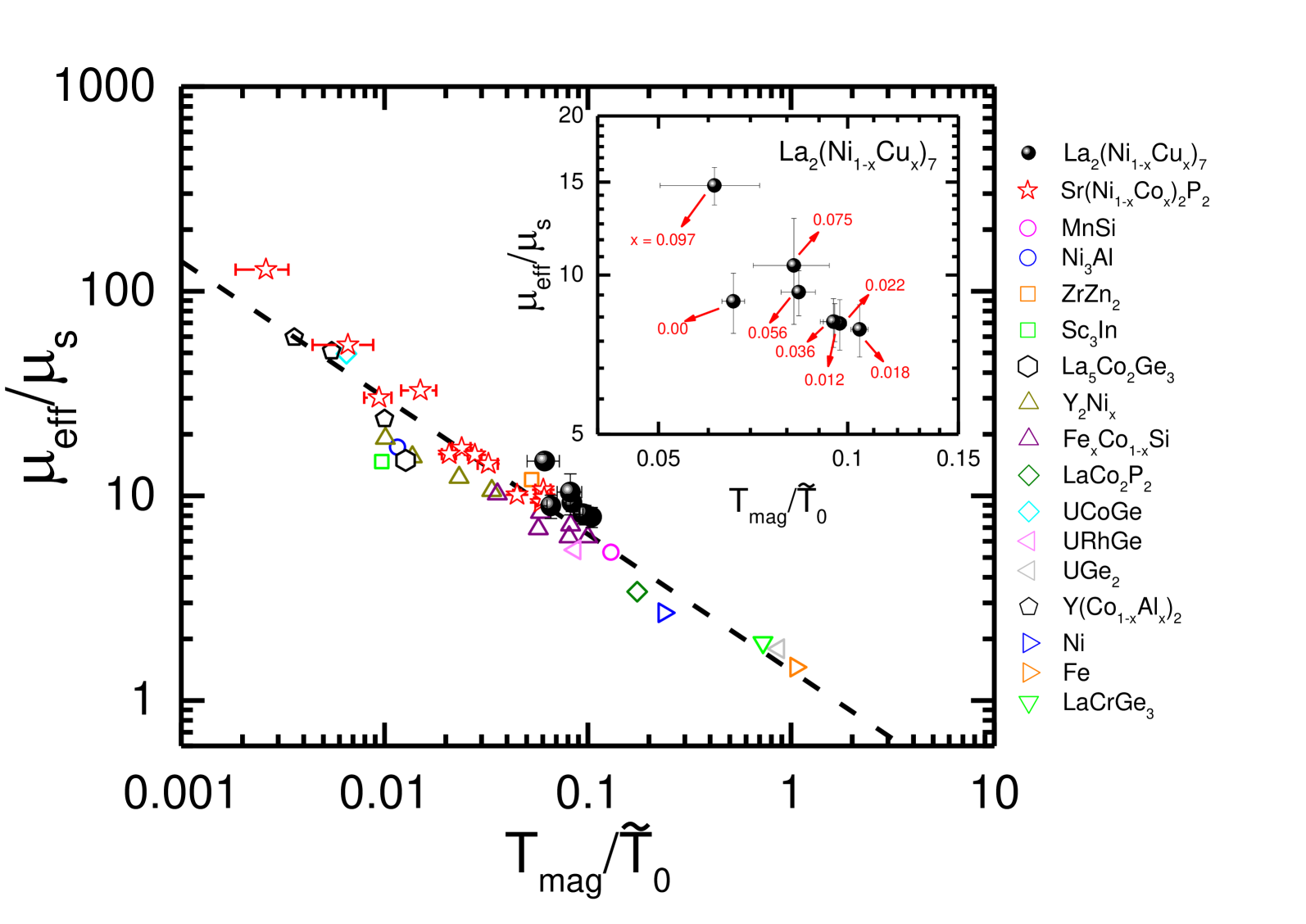
Figure 10: Modified Deguchi-Takahashi plot for La₂(Ni_1-xCu_x)₇ with $0\leq x\leq 0.097$ and other weak itinerant magnets [41, 42, 43, 44]. The dashed line represents the expected theoretical behavior [42]. Inset: enlarged scale showing only the compositions explored in this study, where the labels with red arrows are indicating the Cu fraction corresponding to each point.

To further examine the itinerant character of magnetism in this system we performed a Deguchi-Takahashi analysis [41, 42, 43, 44]. The values of $\mu_{eff}$, $\mu_{s}$, $T_{N}$ and the modified spectral parameter, $\tilde{T}_{0}$, were combined into the modified Deguchi-Takahashi plot as shown in Fig. 10 (black circles). The $M(H)$ data set at $T=1.8$ K for $0\leq x\leq 0.097$ were used to estimate the values of $\tilde{T}_{0}$ as outlined in Ref. [41]. This plot also includes other known itinerant ferromagnets and antiferromagnets [41, 42, 43, 44], as well as a dashed line for the expected theoretical behavior according to Takahashi’s spin-fluctuation therory for itinerant electron magnetism [42]. Since this plot includes both ferromagnets and antiferromagnets, the symbol $T_{mag}$ is used to generally represent $T_{C}$ and $T_{N}$, respectively. The fact that that La₂(Ni_1-xCu_x)₇ with $0\leq x\leq 0.097$ follow the expected trend is a good indication that, despite being antiferromagnetic at zero field, they exhibit typical characteristics of weak itinerant ferromagnets under a finite applied field [45, 46].

Quantum Critical Point, nFL-region and beyond

${\text{La}_{2}\text{(Cu}_{x}\text{Ni}_{1-x})_{7}}$ has a magnetically ordered low temperature state for $x<$ 0.097, whereas we observe a Kondo-like behavior for the higher doped samples. The suppression of both $T_{N}$ and the ordered moment $\mu_{s}$, along with the emergence of apparent Kondo-like behavior in the paramagnetic state suggests that there maybe a quantum critical point in between these two competing regimes. From all the $M(H,T)$, $\rho(T)$, and $C_{p}(T)$ data discussed so far, the $x$ = 0.105 sample appears to be in the vicinity of an AFM-QCP.

Given that the $x$ = 0.105 $\rho(T)$ data appears to be starting to go through a resistive minima upon cooling and then, only at lower temperatures, rolls over into a linearly decreasing $\rho(T)$, it would appear that $x$ = 0.105 may be slightly beyond the critical doping for the precise QCP. A well-established way to examine this is to do a power law analysis of the resistivity data. The $\rho(T)$ data can be analyzed by using,

$$\rho(T)=\rho_{0}+AT^{n}$$ (2)

where $\rho_{0}$ is the residual resistivity and $A$ is a co-efficient and can be interpreted as the quasiparticle scattering cross section. Alternatively, we can use the obtained value of $\rho_{0}$ and plot $\ln{(\rho-\rho_{0})}$ vs $\ln{T}$ for all Cu-substituted samples. A low temperature linear fit can be done to this data which corresponds to,

$$\ln{(\rho-\rho_{0})}=n\ln{T}+\ln{A}$$ (3)

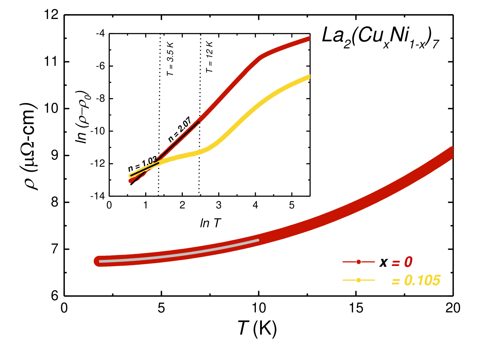
Figure 11: Plot of $\rho(T)$ for the parent $x$ = 0, ${\text{La}_{2}\text{(Cu}_{x}\text{Ni}_{1-x})_{7}}$, with the grey line showing the fit of Eqn. 2. We obtain $\rho_{0}$ from this fit, which can be further used to plot $\ln{(\rho-\rho_{0})}$ vs $\ln{T}$. (Inset: $\ln{(\rho-\rho_{0})}$ vs $\ln{T}$ for $x=0$ and $x=0.105$. A linear fit is done to low temperature data between 1.8 K $\leq T\leq$ 10 K for $x$=0 and 1.8 K $\leq T\leq$ 3.5 K for $x$=0.105 to obtain $n$ and $A$ (See text for details). The fit line is shown in black. The slope of this fit gives the value of $n$ = 2.07(2) for $x$ = 0 and $n$ = 1.03(6) for $x$ = 0.105.)

The slope of the fit gives the value of $n$. In this paper, we have estimated the value of $n$ using both Eqns. 2 and 3, and the values of each are within the uncertainty limit. From this point onwards in this paper, we will refer to the value of $n$ obtained from Eqn 3 only. The exponent, $n$, indicates whether the system is in a Fermi liquid (FL) regime $(n=2)$ where electron-electron scattering is dominant, or, in a nFL $(n\sim 1)$ regime which is the behavior expected in the vicinity of a quantum critical point (QCP) [47].

We perform such an analysis for $x<$ 0.105 samples only. The potential contribution from magnons below the ordering temperature is acknowledged, but given the very small size of the ordered moment, as well as the small resistive anomaly associated with the loss of spin disorder scattering, we assume that magnon scattering is minimal compared to the electron-electron scattering. For the higher doped $0.125\leq x\leq 0.181$ samples, the presence of the low temperature upturn in the data inhibits us from doing such an analysis.

Figure 11 shows the plot of $\rho(T)$ with the fit line to Eqn. 2 for $x$ = 0 and $\ln{(\rho-\rho_{0})}$ vs $\ln{T}$ for the parent compound as well as the other extreme member, $x=0.105$. Similar data are plotted for the other samples are shown in the Appendix in Fig 25. Using Eqn. 3, we obtain $n$ = 2.07 (2) and 1.03 (6) for $x$ = 0 and 0.105 respectively which suggests that the parent $x$ = 0 sample behaves as a Fermi liquid, whereas $n\sim$ 1 for $x$ = 0.105 sample may indicate nFL behavior. We emphasize here that for $x$ = 0.105, the fit could only be performed over a small temperature window. However, it is clear from Fig. 11 that the low temperature behavior of the $x$ = 0.105 sample does not follow a Fermi liquid behavior.

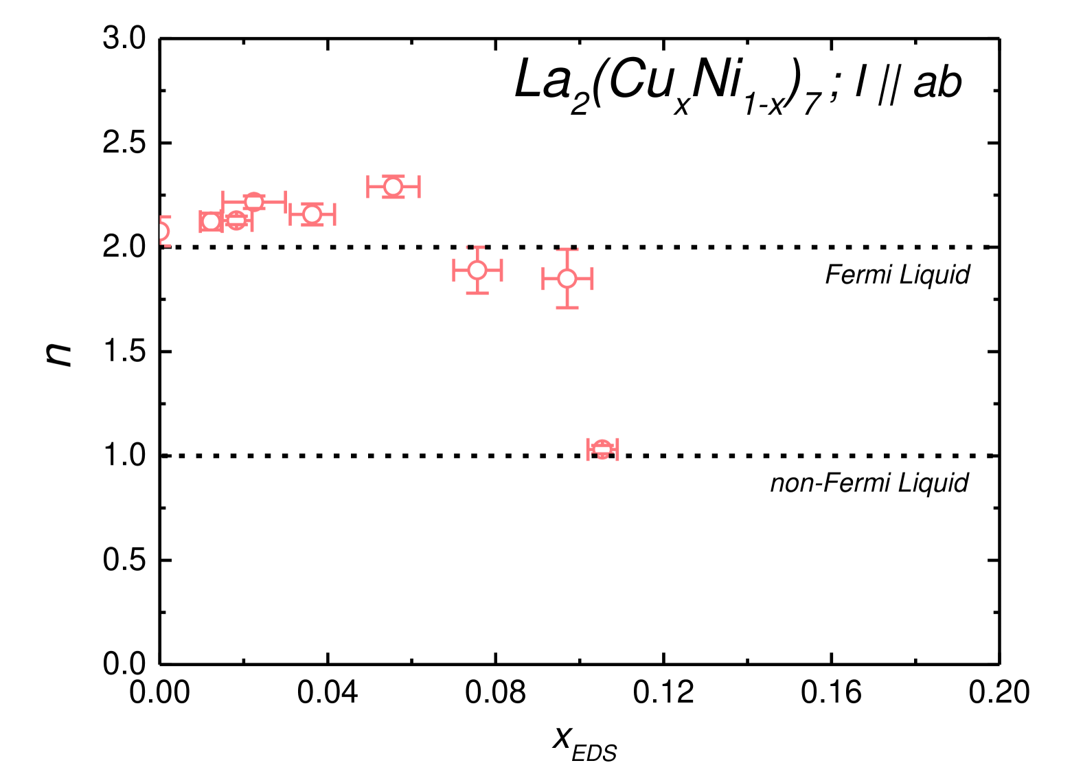
Figure 12: Plot of the slope $n$ of the linear fit to the low temperature $\ln{(\rho-\rho_{0})}$ vs $\ln{T}$ data to the ${\text{La}_{2}\text{(Cu}_{x}\text{Ni}_{1-x})_{7}}$ samples for 0 $\leq x\leq$ 0.105 obtained from their respective zero field, in-plane $\rho(T)$ data. A value of $n$ = 2 corresponds to Fermi liquid behavior whereas $n$ = 1 corresponds to a non-Fermi liquid behavior and is shown using horizontal lines. Values of $n$ for $x>$ 0.105 are not shown due to Kondo-like upturn in their $\rho(T)$ data.

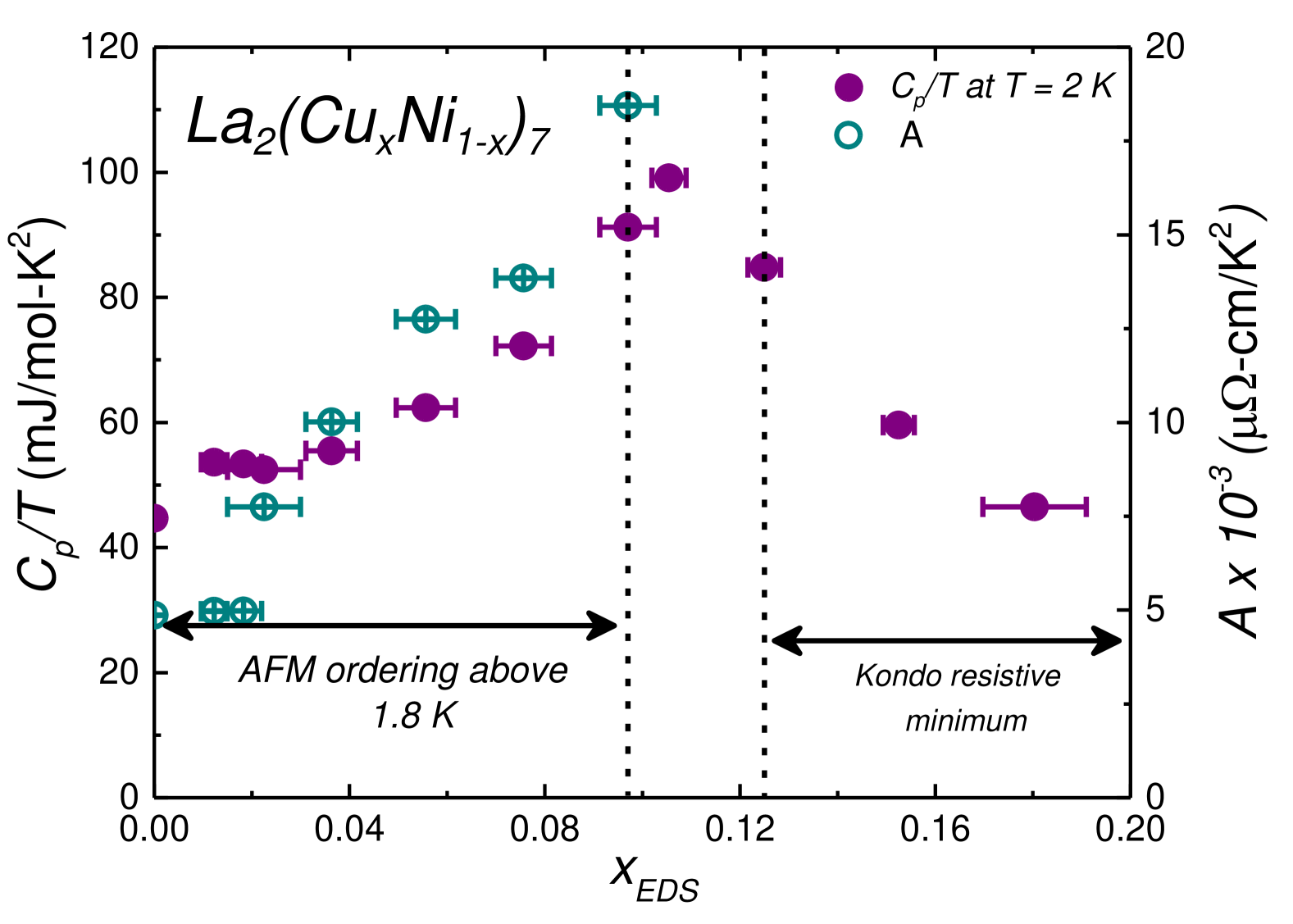
Figure 13: (Color online) ${a}$ Plot of $C_{p}/T$ measured at $T$ = 2.0 K vs $x$ for the ${\text{La}_{2}\text{(Cu}_{x}\text{Ni}_{1-x})_{7}}$ single crystals plotted on the left axis (solid circles) and $A$ obtained from fitting Eqn. 2, with a fixed $n$=2 to the low temperature $\rho(T)$ data on the right axis (hollow circles). The AFM ordered above base temperature ($T$ = 1.8 K) and the Kondo-like regime is marked.

Figure 12 shows the evolution of the slope $n$ of the linear fit to the low temperature $\ln{(\rho-\rho_{0})}$ vs $\ln{T}$ data to the ${\text{La}_{2}\text{(Cu}_{x}\text{Ni}_{1-x})_{7}}$ samples for 0 $\leq x\leq$ 0.105. The value of $n$ is $\sim$ 2 for the magnetically ordered 0 $\leq x\leq$ 0.097 samples and then decreases to a value of 1.03 for $x$ = 0.105, which may suggest nFL behavior for this doping. We again emphasize the limited temperature range used for these fits restrict the confidence with which we can draw conclusions; however, given that the inferred value of $n$ changes rather sharply at the exact Cu concentration for which magnetic order is suppressed, it is reasonably to infer a crossover between Fermi liquid and non-Fermi liquid regimes may occur near $x$ = 0.105.

In order to explore this apparent QCP, we can see how the prefactor $A$ of $\rho(T)~=~\rho_{0}~+AT^{2}$ behaves as we approach $x=$ 0.105 from below. Given that for $x<$ 0.105 we find $n\sim$2, we fit our low temperature $\rho(T)$ data to a classical $T^{2}$ temperature dependence. In Fig. 13 we plot $A$ as a function of $x$ and see that it diverges in a manner very similar to the $C_{p}/T$ data. In fact, we can see in Fig 27, in the Appendix, that our data are consistent with the Kadowaki-Woods scaling of $A$ with $\gamma$, another hallmark of Kondo-like systems.

The $\rho(T)$ behavior for $x$ = 0.105 sample is intermediate to the lower $x$-values, with magnetic ordering and power law exponent values closer to 2, and higher $x$-values which manifest no evidence of magnetic ordering and have a Kondo-like minimum in $\rho(T)$. Re-examining the data for $x$ = 0.105 shown in Fig 5, in the higher temperature range it looks like the $\rho(T)$ will go through a Kondo minimum, but just as it reaches the bottom of the Kondo minimum, it instead transitions into the linear nFL behavior. This suggests that the true QCP $x$-value for this system may be slightly below the $x$ = 0.105 sample we measured.

We further investigate the possible nFL behavior with specific heat measurements. When a system shows nFL behavior in the vicinity of a QCP, an upturn in $C_{p}/T$ at low temperatures and enhanced Sommerfeld coefficient, $\gamma$ are often observed [47]. $\gamma$ is usually obtained from the linear extrapolation of the low temperature $C_{p}/T$ vs $T^{2}$ data to $T$ = 0. But from Fig 6 and Fig 26 in the Appendix, we see that the low temperature upturn makes it difficult to do such extrapolation in a consistent manner.

Figure 13 shows the change of the $C_{p}/T$ value measured at $T$ = 2.0 K with $x$ (left axis). For $x$ = 0, its value is close to the reported value of $\gamma$ at $\sim$ 40 mJ/mol K² [30]. For 0 $\leq x\leq$ 0.075, $C_{p}/T$ increases to $\sim$ 70 mJ/mol K² as expected for a fragile moment (correlated electron) system as its magnetic transition temperature is reduced. For $x$ = 0.097 and 0.105, $C_{p}/T$ increases more rapidly and reaches its maximum value of $\sim$100 mJ/mol-K² for $x$ = 0.105, very close to where we infer the QCP in this system. For the highest dopings 0.125 $\leq x\leq$ 0.181, $C_{p}/T$ decreases monotonically as the upturn in the data decreases and returns toward more linear behavior (See Fig 26).

Although the change in the 2.0 K value of $C_{p}/T$ is smaller than would be expected in the case of QCPs associated with Ce- or Yb- based moments, there is a clear and substantial increase in $C_{p}/T$ that can be expressed as either, ”near doubling” or ”increase by roughly 50 mJ/mol-K². The observation that this peaked increase in $C_{p}/T$ occurs for the $x$-value close to the extrapolation of the suppressed $T_{N}$ line and the $x$- value for which we find nFL-like behavior in the low temperature resistivity strongly suggest that all three of these phenomenon arise from a QCP associated with a d-band based fragile magnetism.

Possible low temperature single-ion Kondo-like region; 0.125 $\leq x\leq$ 0.181

The three highest Cu substituted samples, 0.125 $\leq x\leq$ 0.181, show anomalous low temperature resistivity and specific heat behavior is reminiscent of the Kondo effect. In this section we will discuss this behavior in greater detail.

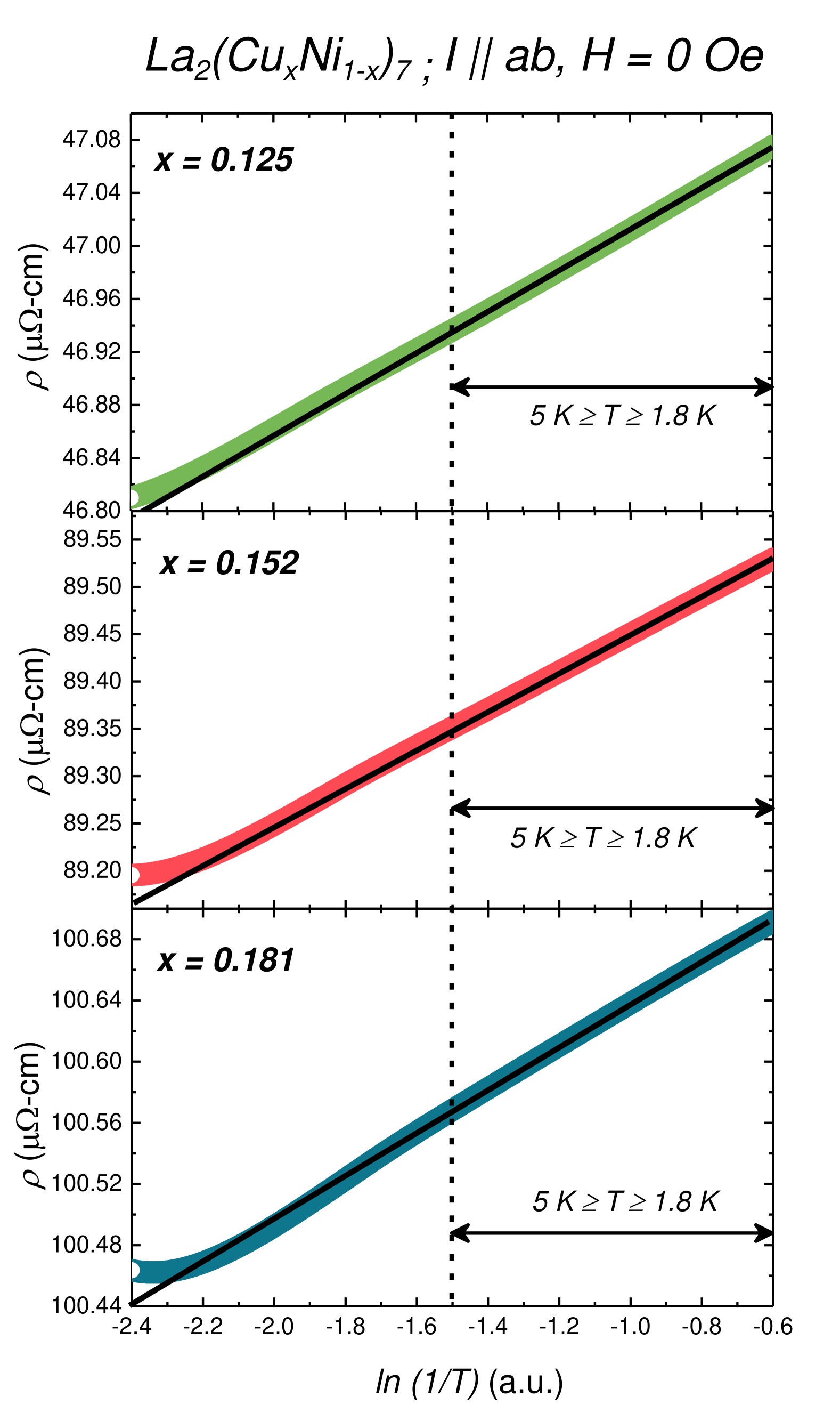
Figure 14: (Color online) Plot of $\rho$ vs $\ln{1/T}$ for $x$ = 0.125, 0.152, and 0.181 ${\text{La}_{2}\text{(Cu}_{x}\text{Ni}_{1-x})_{7}}$ single crystals in the temperature range 1.8 K $\leq x\leq$ 11 K. A linear fit to the temperature range 1.8 K $\leq T\leq$ 5 K, shown using the black line, to each of these data shows a linear $\ln{1/T}$ behavior which is expected for single ion Kondo effect. There is a clear deviation from linearity as we increase the temperature.

Such an increase in the resistivity could in principle have many potential sources. For three-dimensional systems, an increase in resistivity with decreasing temperature should follow either a $T^{-p/2}$ dependence if it is due to weak localization (p = 3/2, 2, 3, depending upon the scattering mechanism) [48, 49, 50], or a $\ln{(1/T)}$ dependence if it is due to the Kondo effect [48, 51, 52]. To ascertain the nature of the low T resistivity upturn in our samples, we plot the resistivity with respect to $T^{-p/2},(p=3/2,2,3)$ and $\ln{(1/T)}$ for $x=0.125,152,$ and 0.181 samples. The data for $\ln{(1/T)}$ behavior is shown in Fig 14 whereas the data plotted against $T^{-p/2}$ dependencies is shown in Fig 28 in the Appendix. A linear fit is done between 1.8 K $\leq T\leq$ 5 K to each of the data sets, and a good fit is only obtained for $\ln{(1/T)}$, suggesting the Kondo effect is indeed the origin of the resistance upturn.

We also measured $\rho(T)$ under an external applied field for both $H\perp c$ and $H\||c$ directions for $x$ = 0.152 sample. If the resistive upturn is due to Kondo scattering, then it is expected to be suppressed gradually with increasing magnetic field as it was observed in the case of weak Kondo effect in $\text{Zr}\text{Te}_{2}$ [51] or $\text{La}_{3}\text{Cu}_{4}\text{P}_{4}\text{O}_{2}$ [53] or the classic Yb-based system [17]. Figure 15 shows the results of $\rho(T)$ under an external field, where the resistance minima is clearly suppressed by the applied field, nearly vanishing at 70 kOe. All together, given that the specific heat as well as the $\rho(T)$ are consistent with Kondo-like behavior, it appears that after the suppression of the fragile magnetism in ${\text{La}_{2}\text{(Cu}_{x}\text{Ni}_{1-x})_{7}}$, a 3d-based single-ion Kondo-like state emerges in this system.

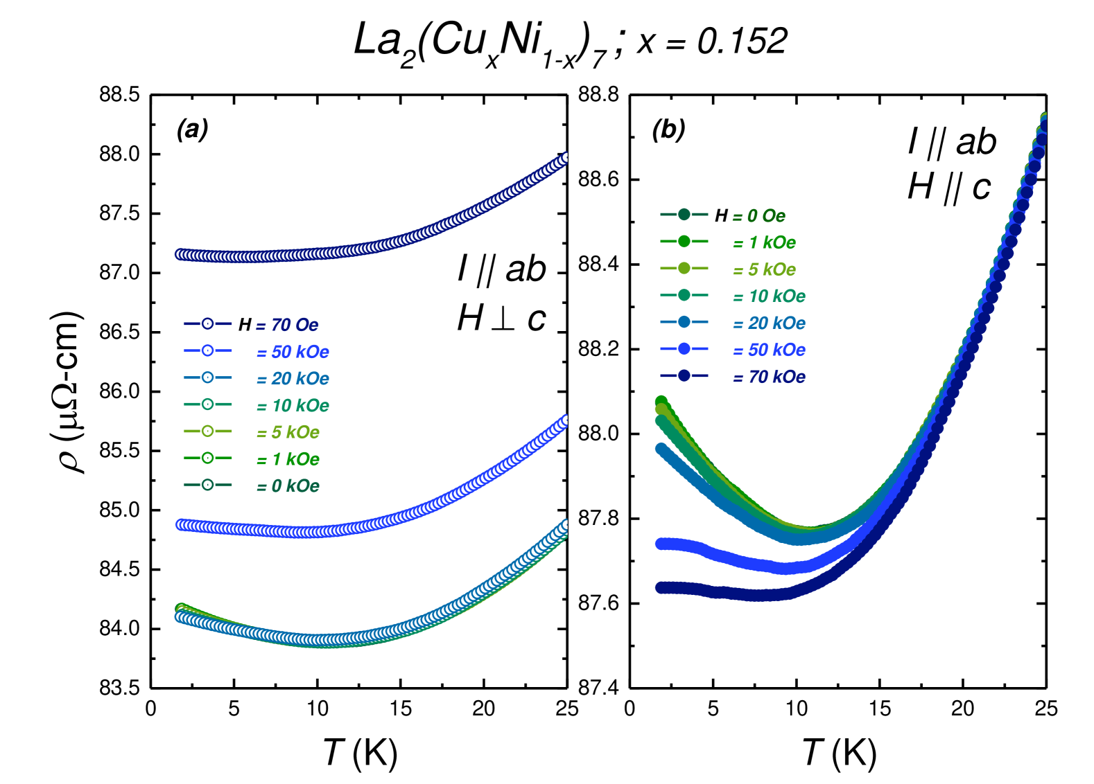
Figure 15: Plot of the transverse temperature dependent resistivity $\rho(T)$ under an external applied magnetic field for $H\perp c$ in panel $(a)$ and $H\||c$ in panel $(b)$ for $x$ = 0.152 ${\text{La}_{2}\text{(Cu}_{x}\text{Ni}_{1-x})_{7}}$ sample. In panel $(a)$, the data sets for 0 kOe $\leq H\leq$ 20 kOe essentially overlap and are not resolvable in this plot.

IV Discussion and Conclusions

To summarize, we synthesized single crystals of ${\text{La}_{2}\text{(Cu}_{x}\text{Ni}_{1-x})_{7}}$ with $x$ varying between 0 and 0.181. Powder x-ray diffraction and EDS measurements confirmed the phase and the concentration of Cu respectively. Based on a suite of anisotropic temperature and field dependent magnetic, transport, and specific heat measurements, we constructed the $T-x$ phase diagram for this system. For 0 $\leq x\leq$ 0.097, the system remains magnetically ordered with transition temperature(s) above ($T$ = 1.8 K) with the parent $x$ = 0 and the lowest doped $x$ = 0.012 showing signs of three magnetic phases $A$, $B$, and $C$ whereas only phase $C$ is observed for the others (0.018 $\leq x\leq$ 0.097). The AFM transition temperatures for all three phases decrease with increase in the Cu substitution level. The high-field saturated moment $\mu_{s}$ and the effective moment $\mu_{eff}$ also decreases with increase in $x$, with $\mu_{s}$ vanishing alongside $T_{N}$. A modified Deguchi-Takahashi analysis on the ${\text{La}_{2}\text{(Cu}_{x}\text{Ni}_{1-x})_{7}}$ series, follows the trend expected for itinerant magnetism under a finite applied field according to Takahashi’s spin-fluctuation theory. In addition, we find that there is good Kadowaki-Woods scaling of $C_{p}/T$ and the $T^{2}$-coefficient $A$, of the low temperature $\rho(T)$; another hallmark of correlated electron behavior. The three highest dopings studied, 0.125 $\leq x\leq$ 0.181, have no magnetic ordering but exhibit an upturn in resistivity with decreasing temperature below $T\sim$ 12 K, which we have interpreted as an indication of a type of Kondo behavior. The sample with an intermediate $x$ = 0.105 is in proximity of the quantum critical regime for this system. As such, then, ${\text{La}_{2}\text{(Cu}_{x}\text{Ni}_{1-x})_{7}}$ is a manifestation of a fragile magnetic system that can be tuned to an AFM-QCP by chemical substitution.

The nFL behavior for $x$ = 0.105 is suggested by power law study to the zero-field $\rho(T)$ and $C_{p}(T)$ data which point to an enhanced electron mass and possible nFL behavior as $x$ approaches $\sim$ 0.1 from both low and high dopings. Analysis of the temperature dependence of $\rho$ shows a $\ln{(1/T)}$ behavior below the resistance minimum, and measurements at different fields show that this minima is weakened with $H$ (Fig. 15). Both of these observations suggest that the Kondo effect is the origin of the anomalous low temperature behavior.

On one hand, the single ion-Kondo effect was first discovered in metals (such as gold) with minute amounts of $3-d$ transition metal impurities (such as Fe) [54]. On the other hand, Kondo physics, manifested by an anomalous upturn in resistivity data [55] in the vicinity of a QCP is traditionally associated with rare earth, especially Ce or Yb, atoms in intermetallic compounds, where the localized $f$ -orbitals hybridize with the surrounding $s-,~p-,$ or $d-$ orbital bands often revealing exotic phenomenon such as unconventional superconductivity, non-Fermi liquid, etc. [8]. Thus, the observation of Kondo-like behavior when tuning a purely $3d$ system is surprising. It is interesting to consider whether this behavior may be rooted in the kagome network formed from the Ni4 and Ni5 atoms (See Fig.1). Compact localized states associated with the kagome structure have been suggested to produce orbital currents that may act like localized moments and have been proposed to provide a mechanism for $d-$ band based Kondo physics [56, 57]. This said, having a d-shell based fragile magnetic system, by itself, is not unusual; the curious, and still unexplained, aspect of the ${\text{La}_{2}\text{(Cu}_{x}\text{Ni}_{1-x})_{7}}$ system is the change from Fermi-liquid like resistivity for low $x$ that evolves to a nFL-like behavior near a QCP to a single-ion Kondo type of resistance for $x>0.105$. Usually after the suppression of the AFM ordering and the quantum critical region, there is another Fermi-liquid region with the putative Kondo temperature rising and the $T^{2}$ coefficient (and $\gamma$) dropping. In the case of ${\text{La}_{2}\text{(Cu}_{x}\text{Ni}_{1-x})_{7}}$, for $x>0.105$ we find that the $\rho(T)$ behavior that has more resemblance to a system in the single ion Kondo impurity limit. Operationally, this simply means that any putative coherence temperature for the Kondo-lattice has dropped below our base temperature, but even with this said, x   0.1 would seem to be a small doping level for this to happen at. One possible explanation is associated with the fact that $\text{La}_{2}\text{Ni}_{7}$ has two of the 5 Ni-sites forming Kagome-like layers. These two Kagome layers accommodate only 9 of the 42 Ni-sites per unit cell. If we were to assume that the fragile moment behavior is coming from the Kagome layers, and if we assume that the Cu preferentially occupies these sites, then $x>0.105$ may feasibly lead to Ni concentrations of these sites moving to the single ion limit. Neutron diffraction experiments will be needed to see if such a preferential occupation of the Ni4 and Ni5 sites by Cu occurs.

Regardless of the origin of the single-ion Kondo-like resistivity behavior for $x>0.105$, or perhaps because of it, our detailed work on the ${\text{La}_{2}\text{(Cu}_{x}\text{Ni}_{1-x})_{7}}$ system firmly identifies it as an interesting family for the study of d-shell based AFM-QCP. In addition, this system offers the possibility of examining the role of Ni-Kagome-layers in the moment formation, ordering and possible single ion Kondo scattering.

APPENDIX

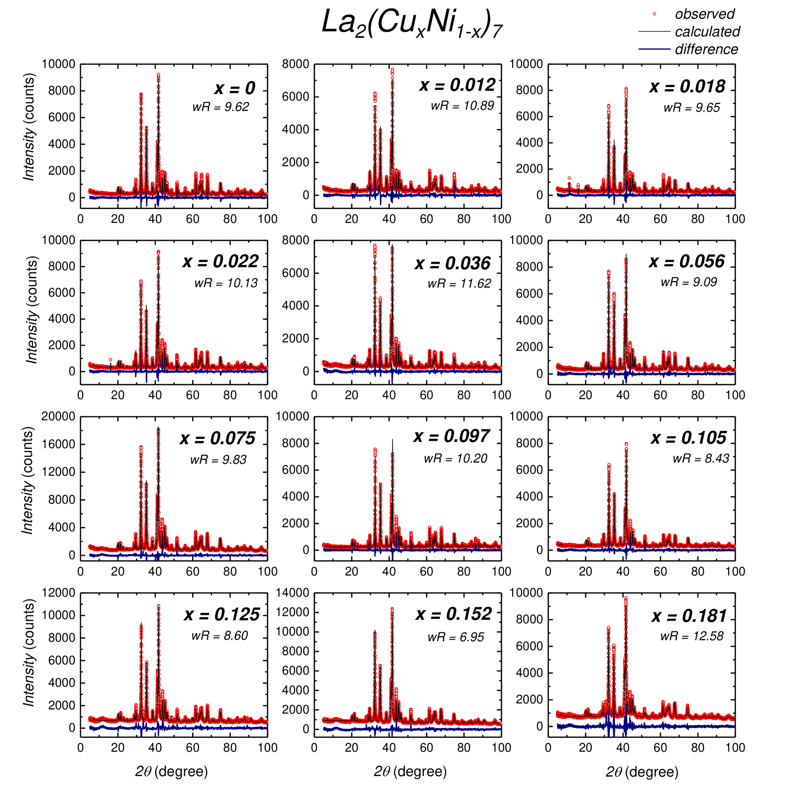
Figure 16: (Color online) Plot of the room temperature powder x-ray patterns of the ${\text{La}_{2}\text{(Cu}_{x}\text{Ni}_{1-x})_{7}}$ samples in separate panels. The patterns are refined using GSAS-II. The difference between the observed and the calculated data is shown in blue in each panel. The wR to each data is mentioned. The data for $x$ = 0.105 is the same as that in the main text in Fig 2.

Powder x-ray patterns of all the Cu substituted samples of ${\text{La}_{2}\text{(Cu}_{x}\text{Ni}_{1-x})_{7}}$ were refined (unit cell, sample displacement,etc. of the atoms) using the Rietveld method and the lattice parameters ($a,~c,\text{V}$) were obtained. In the main text we have shown the change in these parameters with $x$ in Fig 3. Here we show the values of lattice parameters ($a,~c,\text{V}$) and the associated uncertainties in Table 1. Figure 16 shows the observed x-ray patterns after refinement and the residual showing the goodness of the refinement. $wR$ also helps to parametrize the quality of the refinement. The data for $x$ = 0.105 were already shown in the main text.

Figure 17: (Color online) Plot of polycrystalline averaged $\frac{d(\chi T)}{dT}$ at an external field of $H$=100 Oe and in-plane, zero field $\frac{d\rho}{dT}$, for the ${\text{La}_{2}\text{(Cu}_{x}\text{Ni}_{1-x})_{7}}$ single crystals which show magnetic transitions (Fig. 4) and (Fig. 5). The AFM magnetic transition temperatures, $T_{N}$ for these Cu doped samples are determined using both polycrystalline $\frac{d(\chi T)}{dT}$ and $\frac{d\rho}{dT}$ (See text for details). The vertical line in each panel is the $T_{N}$ determined from the $M(T)$ data and agree with that obtained from the $\rho(T)$ data especially for the lower $x$-values. The parent compound ($x$=0) and lowest doped ($x$=0.012) show signs of three transitions whereas the other doped systems show only one.

$x$	$a(\AA )$	$c(\AA )$	$V(\AA )^{3}$	wR
0	5.0585(11)	24.667(3)	545.36(19)	9.62
0.012(2)	5.0588(29)	24.667(9)	546.82(26)	10.89
0.018(4)	5.0624(15)	24.687(4)	547.93(22)	9.65
0.022(9)	5.0602(9)	24.679(3)	547.27(16)	10.13
0.036(5)	5.0654(8)	24.681(3)	548.38(17)	11.62
0.056(6)	5.0655(9)	24.707(3)	549.03(56)	9.09
0.075(6)	5.0651(18)	24.700(6)	549.76(31)	9.83
0.097(6)	5.0719(7)	24.719(7)	550.48(13)	10.20
0.105(3)	5.0729(27)	24.727(4)	551.09(21)	8.43
0.125(7)	5.0729(15)	24.732(1)	551.11(25)	8.60
0.152(6)	5.0811(12)	24.748(4)	553.35(14)	6.95
0.181(11)	5.0899(16)	24.780(3)	555.68(24)	12.58

Table 1: The values of the lattice parameters $a$, $c$, and the volume of the unit cell V of the different $x$ in ${\text{La}_{2}\text{(Cu}_{x}\text{Ni}_{1-x})_{7}}$ with the values of $x$ obtained from EDS measurements in the leftmost column. As ${\text{La}_{2}\text{(Cu}_{x}\text{Ni}_{1-x})_{7}}$ manifests a hexagonal unit cell, the lattice parameters $a$ and $b$ are equal. The associated uncertainties are indicated in the respective parentheses. The wR parameter is the goodness of the fit obtained.

$x$	$\mu_{S}$		$\mu_{eff}$	$\Theta_{CW}$	$\chi_{0}(\times 10^{-5})$
	$(\mu_{B}/TM)$		$(\mu_{B}/TM)$	$(K)$	emu/mol-TM
	$T$=1.8 K			$H$=20 kOe
	$H||c$	$H\perp c$		poly avg
0	0.092(7)	-	0.84(9)	-71.5(3)	-4.1(8)
0.012	0.097(3)	0.100(4)	0.80(6)	-75.1(2)	-3.4(3)
0.018	0.099(2)	0.105(3)	0.78(9)	-75.4(4)	-2.1(6)
0.022	0.092(2)	0.096(2)	0.75(8)	-74.4(3)	-1.1(5)
0.036	0.088(8)	0.091(1)	0.72(7)	-71.6(3)	4.2(4)
0.056	0.074(1)	0.073(2)	0.66(6)	-61.7(4)	3.9(2)
0.075	0.054(1)	0.056(1)	0.57(12)	-45.9(15)	6.3(9)
0.097	0.029(4)	0.036(4)	0.53(4)	-32.1(4)	8.0(7)
0.105	0.022(5)	0.023(5)	0.49(5)	-17.7(6)	6.9(8)
0.125	0.014(4)	0.014(5)	0.47(4)	-11.9(14)	8.7(8)
0.152	0.004(4)	0.004(4)	0.29(4)	-9.3(16)	17.3(7)
0.181	0.001(3)	0.001(4)	09(5)	-1.3(12)	26.3(13)

Table 2: The values of the extrapolated moment $\mu_{S}$, effective moment $\mu_{eff}$, Weiss temperature $\Theta_{CW}$ and $\chi_{0}$ obtained from the magnetization measurements on the ${\text{La}_{2}\text{(Cu}_{x}\text{Ni}_{1-x})_{7}}$ single crystals. $\mu_{S}$ is obtained from $M(H)$ measurements at 1.8 K and has distinct values along $H||c$ and $H\perp c$ whereas the other parameters ($\mu_{eff}$, $\Theta_{CW}$ and $\chi_{0}$) are obtained from the Curie-Weiss fit to the polycrystalline average of the $M(T)$ data taken at an applied field of 20 kOe. The uncertainties associated with each parameter is shown in the respective parentheses.

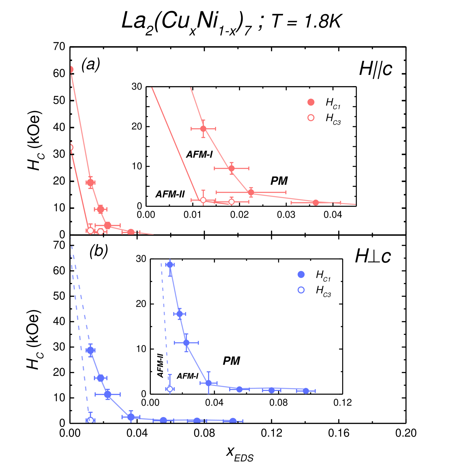
Figure 18: The metamagnetic transition field $H_{C}$ vs $x$, obtained from the $M(H)$ data measured at T=1.8 K for both (a) $H||c$ and (b) $H\perp c$ for ${\text{La}_{2}\text{(Cu}_{x}\text{Ni}_{1-x})_{7}}$ single crystals. The data has been measured for increasing magnetic field. The insets to both the panels show the low $x$ behavior up to which $H_{C}$ is suppressed. For both $H||c$ and $H\perp c$ direction, we observe two magnetically ordered regimes which are labeled as $(AFM-I)$ and $(AFM-II)$ areas. The lines are drawn as guide to the eye. $H_{C1}$ and $H_{C3}$ for $x=0$ for $H\perp c$ direction is $>$ 70 kOe as shown in [30] and is not marked in this plot. We extrapolate the guide lines (dashed lines) for this direction to H$>$ 70 kOe for $x=0$.

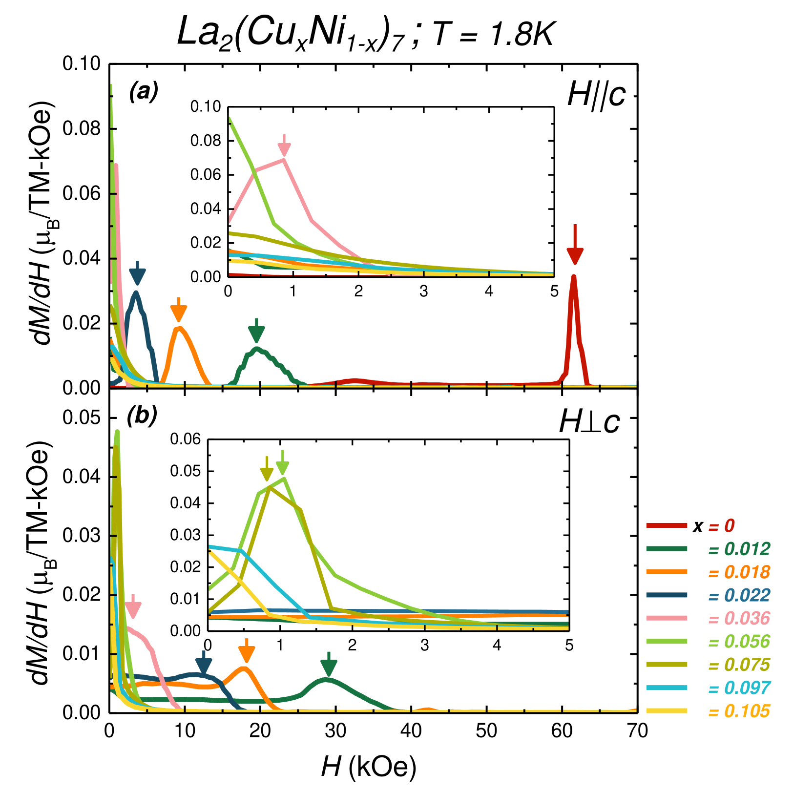
Figure 19: (Color online) Derivative of the anisotropic $M(H)$ with respect to $H$ measured at $T$ = 1.8 K for the magnetically ordered single crystals of ${\text{La}_{2}\text{(Cu}_{x}\text{Ni}_{1-x})_{7}}$, for both $H||c$ in panel $(a)$, and $H\perp c$ in panel $(b)$ respectively. For $H\perp c$ direction. The inset to both the panels shows the low field behavior for clarity, especially for the higher doped samples.

The magnetic transition temperature $T_{N}$ of the lower doped ${\text{La}_{2}\text{(Cu}_{x}\text{Ni}_{1-x})_{7}}$ samples (0 $\leq x\leq$ 0.097) is determined from the $\frac{d(\chi T)}{dT}$ at 100 Oe, zero field $\frac{d\rho}{dT}$ and zero field $C_{p}(T)$ data. Fig 17 shows the polycrystalline averaged $\frac{d(\chi T)}{dT}$ obtained by measuring anisotropic $M(T)$ at $H$ = 100 Oe. Not only the signatures of three transitions for $x$ = 0 and 0.012, but also the single transition for the other substitutions are clearly observed in the data. The value of $T_{N}$ obtained from $M(T)$ is similar to that obtained from the $\rho(T)$ measurements; we have included the $\frac{d\rho}{dT}$ (originally shown in Fig. 5 in the main text) data for easier comparison.

Field dependent $M(H)$ measured at the base temperature ($T$ = 1.8 K) (Fig 8) has signatures of metamagnetic transitions for 0 $\leq x\leq$ 0.097 samples. The presence of metamagnetic transitions in the $M(H)$ data confirms an antiferromagnetic magnetic order in the system at this temperature. We track the change of the metamagnetic transition field $H_{C}$ with $x$ in Fig. 18. We will refer to the higher field transition as $H_{C1}$ and the lower field one as $H_{C3}$. $H_{C}$ is obtained from the peak in the $\frac{dM}{dH}$ plot which is shown in Fig 19.

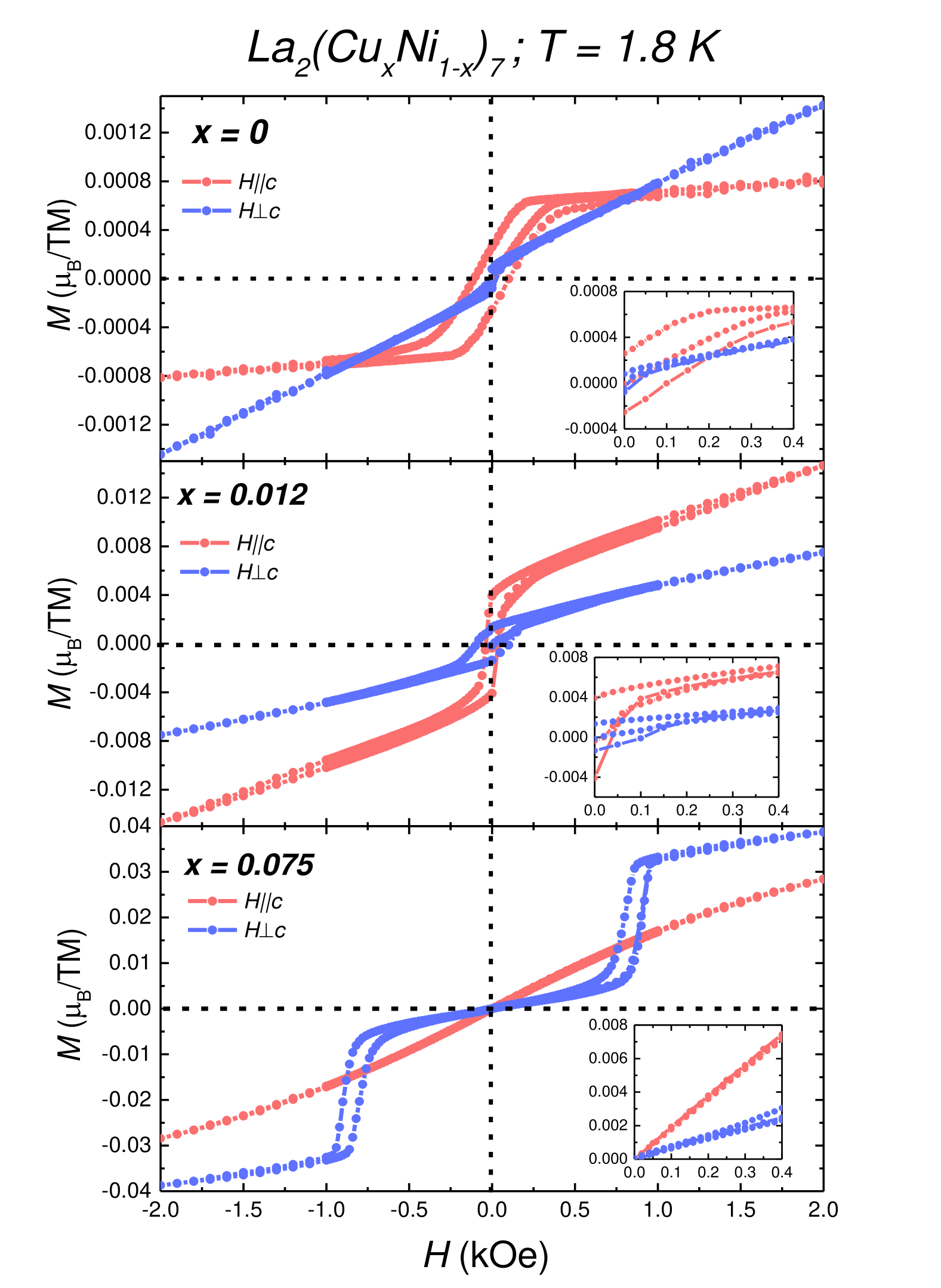
Figure 20: 5 segment $M(H)$ measured at $T$ = 1.8 K for the parent ($x$ = 0) as well as $x$ = 0.012 and 0.075 ${\text{La}_{2}\text{(Cu}_{x}\text{Ni}_{1-x})_{7}}$ for both $H||c$ and $H\perp c$ directions. (Inset to each panel shows the zoomed in data to show the low field feature.

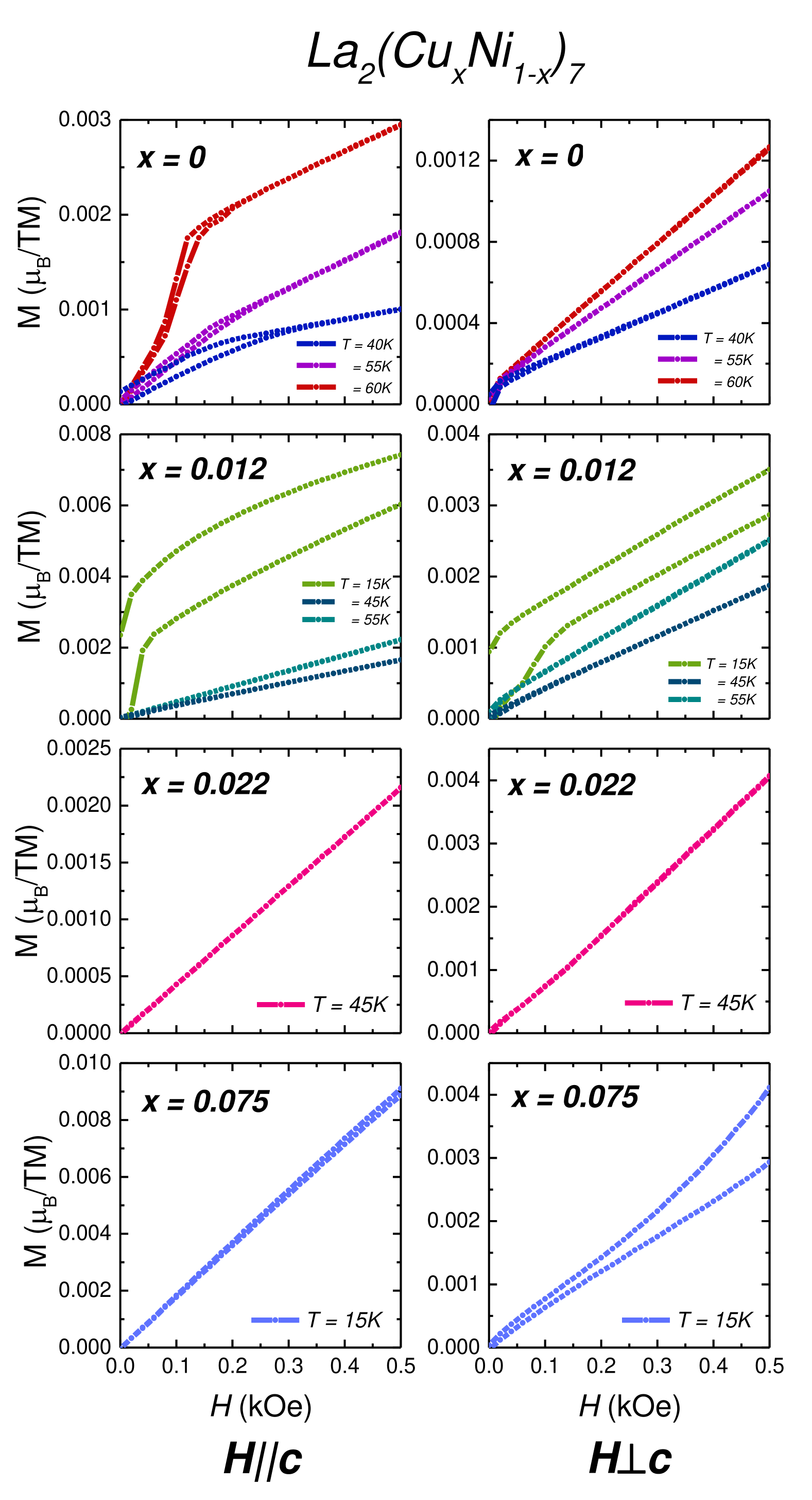
Figure 21: $M(H)$ measured at temperatures slightly below the transition temperatures for $x$ = 0, 0.012, 0.022, and 0.075 for both $H||c$ and $H\perp c$ directions. $M(H)$ is measured for both increasing and decreasing field directions to test for possible FM component to the AFM transition.

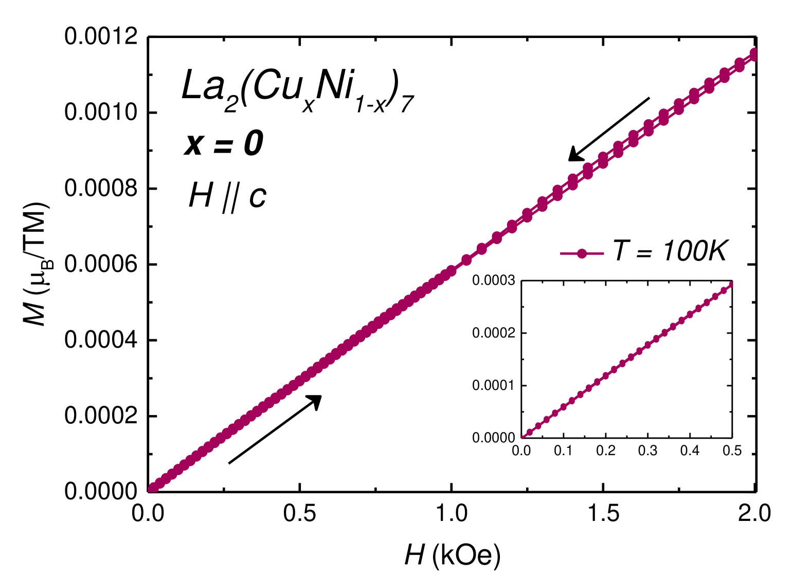
Figure 22: $M(H)$ for the parent $x$ = 0 measured at $T$ = 100 K for $H||c$ direction. The data was measured for both increasing and decreasing fields. (Inset: zoomed in data to show the low field behavior for clarity.)

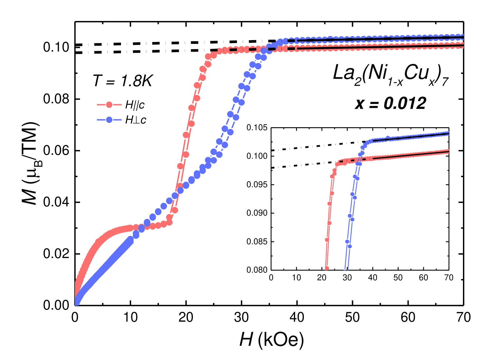
Figure 23: The extrapolated moment $\mu_{s}$, obtained by extrapolating the high-field behavior to zero field for $x$ = 0.012 for both $H||c$ and $H\perp c$. The black line intercepting the $y-$ axis is the value of the extrapolated moment. $\mu_{s}$ for all other $x$ in ${\text{La}_{2}\text{(Cu}_{x}\text{Ni}_{1-x})_{7}}$ are also obtained in the same manner. The inset shows the zoomed in y-axis to highlight the higher field behavior.

From the anisotropic $H_{C}-x$ phase diagram, we observe that $H_{C}$ is suppressed by $x\sim$ 0.04 for $H||c$ whereas at a higher doping level of $x\sim$ 0.10 for $H\perp c$. However for both directions we observe a lower field AFM region suppressed by $x\sim$ 0.012. The two magnetically ordered regimes are shown in Fig 18. For both directions, the higher [lower] field region will be referred as $AFM-I$ [$AFM-II$] respectively. The low dopings (0 $\leq x\leq$ 0.012) exhibit more than one ordered regime ($A,B$ and $C$ in the $T-x$ and $AFM-I,AFM-II$) in the $H_{C}-x$) and the higher Cu doped samples exhibit only a single AFM regime. Neutron diffraction studied will be important to determine the exact character of the magnetic ordering as a function of $x$ and $T$.

Given that we find finite ZFC-FC splitting in the 100 Oe $M(T)$ data as shown in Fig. 4 for lower $x$ concentrations, at low temperatures, we measured a 5-quadrant $M(H)$ at the base temperature of 1.8 K for $x$ = 0, 0.012, and 0.075 for both $H||c$ and $H\perp c$ directions which is shown in Fig 20. The data for $x$ = 0 and 0.012 have a more significant hysteresis in their base temperature $M(H)$ isotherms for both directions whereas for $x$ = 0.075 no observable hysteresis is seen at $H$ = 0. It should be noted that as the low field extrapolation of $H$ goes to zero, saturated moment associated with the apparent FM component is 06 $\mu_{B}/TM$ for the parent $x$=0. This is an order of magnitude smaller than the weak FM component inferred for the higher temperature $C$ phase ($\sim 0.05\mu_{B}/TM$) [30]. As such then, this seems to be a remarkably small component. We speculate that this may well be associated with dislocations of defects in the non-trivial magnetic, long wavelength antiferromagnetic order.

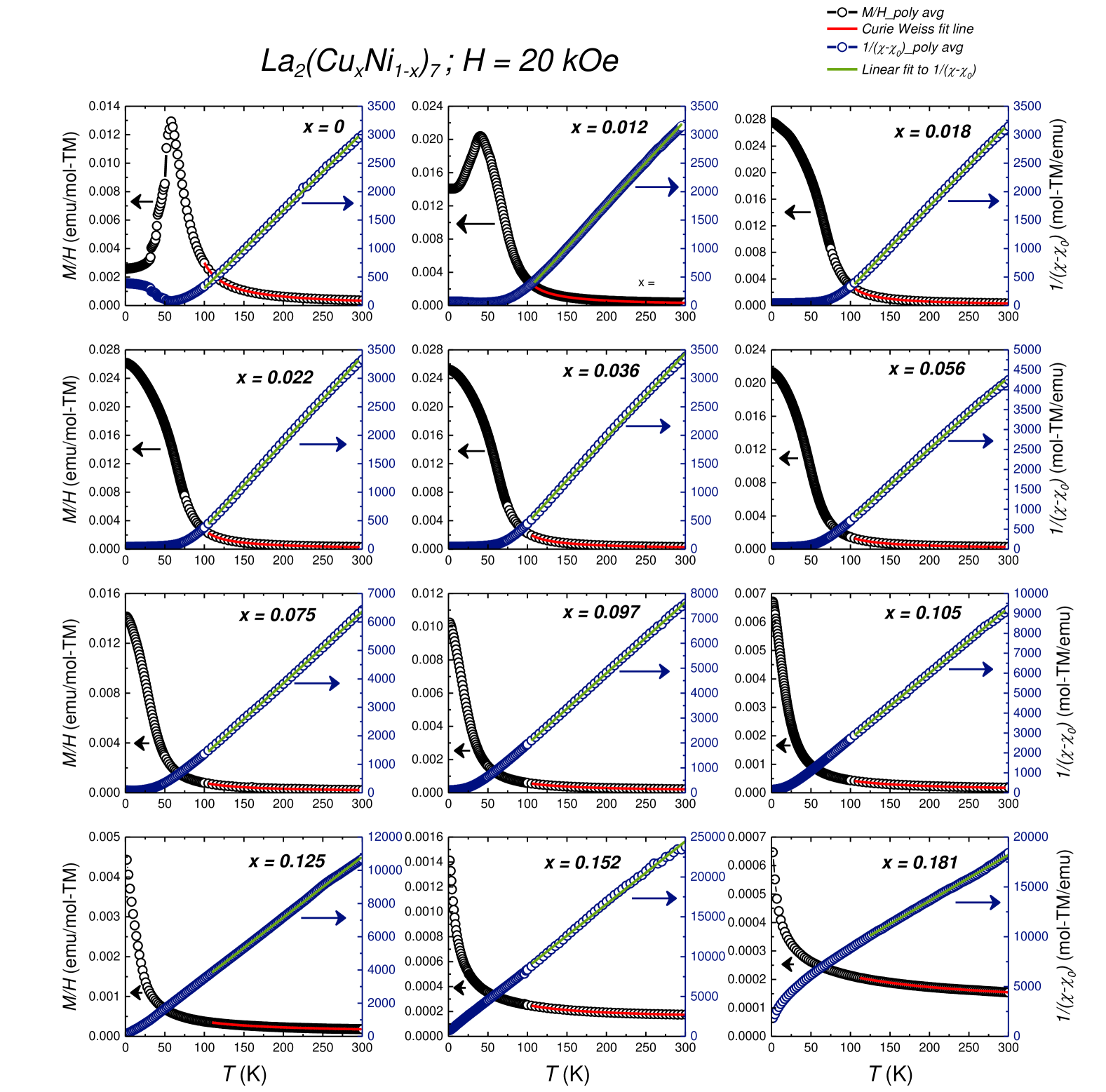
Figure 24: Temperature dependent magnetization $(M(T))$ measured at $H$ = 20 kOe presented as the polycystalline average along the left axis and $(\chi-\chi_{0})^{-1}$ along the right axis for the ${\text{La}_{2}\text{(Cu}_{x}\text{Ni}_{1-x})_{7}}$ single crystals shown in separate panels. The procedure to obtain the poly avg $(M(T))$ data is described in the main text. A Curie-Weiss like fit, as described by Eqn 1 is used in the high temperature regime (100 K $\leq T\leq$ 300 K) of the $M(T)$ data and the fit line is shown in red. The obtained value of $\chi_{0}$ from the fit is used to plot $(\chi-\chi_{0})^{-1}$ for each Cu substitution and is expected to have linear behavior. A linear fit in the same temperature range (100 K $\leq T\leq$ 300 K) is done to the $(\chi-\chi_{0})^{-1}$ plots and is shown using a green line.

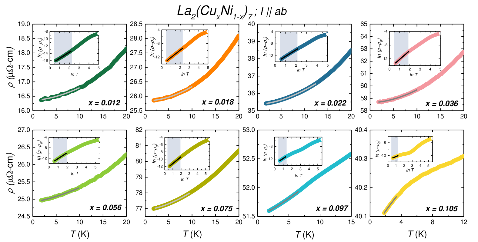
Figure 25: Low temperature $\rho(T)$ data for 0.012 $\leq x\leq$ 0.105 ${\text{La}_{2}\text{(Cu}_{x}\text{Ni}_{1-x})_{7}}$ samples, shown using colored curves and the fit to Eqn. 2 shown using a grey line. We obtained $\rho_{0}$ from these fits and used to plot $\ln{(\rho-\rho_{0})}$ vs $\ln{T}$ for each of these substitutions as shown in the respective insets. A linear fit corresponding to Eqn. 3, shown in black is done to the $\ln{(\rho-\rho_{0})}$ vs $\ln{T}$ plots. The slope and the y-intercept of these linear fits give us values of $n$ and $A$. The temperature range over which we do the linear fit is shown using the grey area in the inset.

Figure 21 addresses the question whether there is a FM component to the AFM magnetic ordering that is found just below the highest (or only) transition temperature for representative Cu substituted samples. We measure $M(H)$ at temperatures slightly below the AFM transition temperatures for $x$ = 0, 0.012, 0.022, and 0.075 for both increasing and decreasing field directions. After demagnetization, the sample was cooled and then data was collected for increasing and then decreasing the field to 0. For $x$ = 0, and 0.012, although the most significant split in the data occurs at the lowest $T$ phase (measured at $T$ = 40 K and 15 K respectively), a much smaller but observable split is seen for the higher $T$ states also for both $H||c$ and $H\perp c$ directions. For the two higher dopings $x$ = 0.022, and 0.075, the situation is slightly different. We do not observe any split in the data for $x$ = 0.022 taken at $T$ = 45 K but a small split is seen for $x$ = 0.075 measured at $T$ = 15 K only for the $H\perp c$ direction.

$M(H)$ for the parent ${\text{La}_{2}\text{Ni}_{7}}$ was also measured at the paramagnetic regime at a temperature of $T$ = 100 K and to confirm the absence of any magnetic impurity with a $T_{C}$ higher than 100 K that could lead to the small FM signal we find. Figure 22 shows the $M(H)$ for $x$ = 0 measured at $T$ = 100 K for both increasing and decreasing fields for $H||c$ direction only. The data has no finite moment and resembles that of a system in non-FM state suggesting that the FM component is magnetic phase $A$ for $x$ = 0 and 0.012 is intrinsic in nature. Thus, from the measurements shown in Figs 20-22 we get an indication that all three magnetic phases ($A$, $B$, and $C$) for $x$=0 and 0.012, and phase $C$ for the other Cu-doped samples may have a small FM component associated with the primary AFM phase. We may speculate this arises due to AFM domain wall and stacking faults in the long wavelength of the AFM ordered phase.

The extrapolated moment, $\mu_{s}$ can be estimated as a proxy for the saturated moment in an itinerant magnetic system. We obtain $\mu_{s}$ by doing a linear fit to the high field (40 kOe $\leq H\leq$ 70 kOe) $M(H)$ data, except for the parent $x$ = 0 where we used 60 kOe $\leq H\leq$ 70 kOe as the interval. The $H$ = 0 intercept of this fit gives the value of $\mu_{s}$. Figure 23 shows the procedure of obtaining $\mu_{s}$ for $x$ = 0.012 as an example. $\mu_{s}$ for all the other ordered samples (0 $\leq x\leq$ 0.097) is obtained in a similar manner and are plotted in Fig 9 of the main text.

We have shown the change of the effective moment with $x$ for ${\text{La}_{2}\text{(Cu}_{x}\text{Ni}_{1-x})_{7}}$ samples in Fig 9. $\mu_{eff}$ is obtained from doing a Curie-Weiss fit to the polycrystalline $M(T)/H$ data which has been already been explained in details in the main text. Figure 24 shows the polycrystalline $M(T)$ data measured at $H$ = 20 kOe along with the Curie-Weiss fit line described by Eqn. 1 for the ${\text{La}_{2}\text{(Cu}_{x}\text{Ni}_{1-x})_{7}}$ samples. CW fit is done over the temperature range 100 K $\leq T\leq$ 300 K and the fit is shown using a red line. To visualize the quality of the fit we plotted $1/(\chi-\chi_{0})$ vs $T$ after obtaining $\chi_{0}$ from Eqn. 1. $1/(\chi-\chi_{0})$ vs $T$ should be linear in the same temperature range as that of the CW fit (100 K $\leq T\leq$ 300 K) as shown using a green line confirming that the polycrystalline average $M(T)$ data at $H$ = 20 kOe clearly follows the Curie-Weiss behavior. The values of all these parameters are shown in Table 2. The values for the parent $x$ = 0 in Ref [30] were obtained from doing a CW fit to the data at $H$ = 1 kOe.

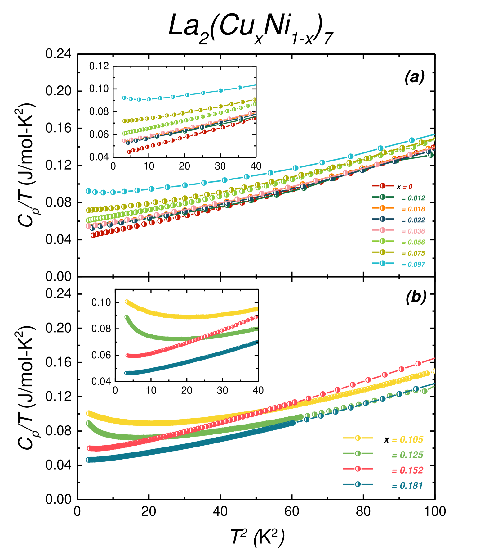
Figure 26: (Color online) Plot of $C_{p}/T$ vs $T^{2}$ for the ${\text{La}_{2}\text{(Cu}_{x}\text{Ni}_{1-x})_{7}}$ samples divided into two separate panels based on their low T behavior. Panel $(a)$ shows the low doped 0 $\leq x\leq$ 0.097 which are almost linear down to the lowest measured temperature. The inset shows the zoomed in data for clarity. Panel $(b)$ shows the $C_{p}$ vs $T^{2}$ data for 0.105 $\leq x\leq$ 0.181 which is no longer linear and has a low T upturn. The insets shows the low T data for $T^{2}\leq$ 40 K for clarity.

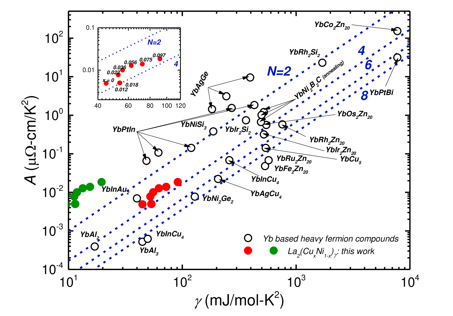
Figure 27: (Color online) Plot of Kadowaki-Woods behavior of Yb-based systems with our data on ${\text{La}_{2}\text{(Cu}_{x}\text{Ni}_{1-x})_{7}}$ plotted on it twice. Once for simple per-mole-f.u.(red circles) and a second time where we have $\gamma$ in terms of per-mole Ni-on Kagome plane (i.e. multiply $\gamma$ by 9/42) (green circles). The inset shows the data for our system identifying the $x$ values. The data for the Yb-based systems have been taken from [58]. The $N$ values shown in the plot refer to the amount of degeneracy (for example, associated with Yb-CEF splitting) that is hybridized into correlated electron state by the Kondo-effect.

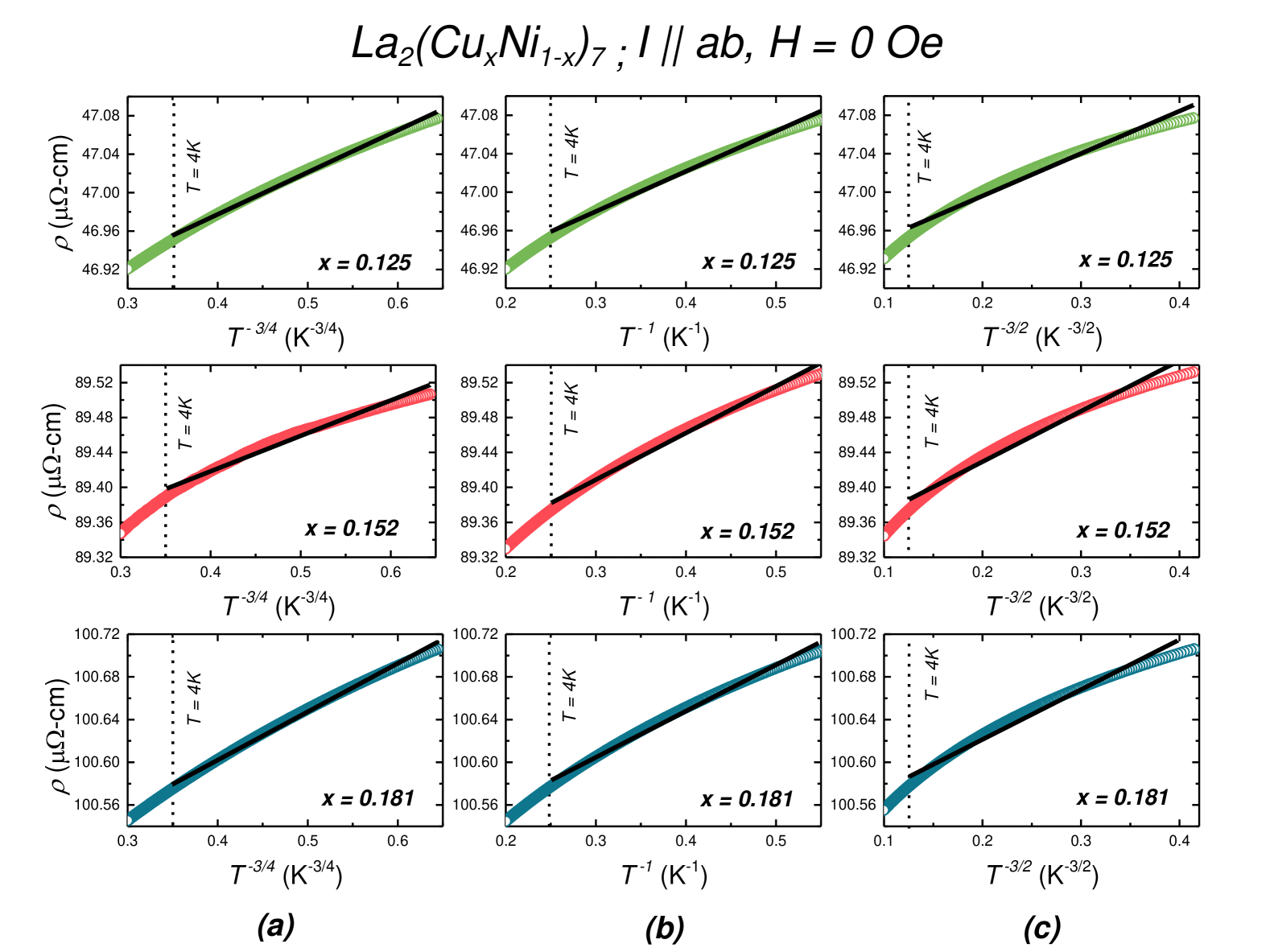
Figure 28: (Color online) Plot of resistivity vs $T^{-3/4}$ in Col$(a)$, $T^{-1}$ in Col$(b)$, and $T^{-3/2}$ in Col$(c)$, for $x=0.125,0.152,$ and $0.181$ single crystals. These particular Cu substitutions show upturn in resistivity with decreasing T (See Fig 5 in the main text). In each of these panels we mark the corresponding $T$ = 4 K value for reference. To verify the temperature dependence and subsequently the nature of the low T upturn, we do a linear fit to each of the panels in the temperature range 1.8 K $\leq x\leq$ 4 K. The linear fit line is shown using the black line. The low T upturn in resistivity is linear in $\ln{1/T}$ as seen in Fig 14 and not in any of the following T dependencies and is thus due to Kondo effect in the ${\text{La}_{2}\text{(Cu}_{x}\text{Ni}_{1-x})_{7}}$ crystals for $x=0.125,0.152,$ and $0.181$.

In the main text we explained the power law analysis of the resistivity data. A fit to Eqn. 2 was shown only for the parent compound ($x$ = 0). In Fig. 25 we show such a fit for 0.012 $\leq x\leq$ 0.105 ${\text{La}_{2}\text{(Cu}_{x}\text{Ni}_{1-x})_{7}}$ samples. We obtain $\rho_{0}$ from these fits, and use those values to plot $\ln{(\rho-\rho_{0})}$ vs $\ln{T}$. A linear fit corresponding to Eqn. 3 is done on the $\ln{(\rho-\rho_{0})}$ vs $\ln{T}$ to obtain $n$ and $A$. Figure 12 shows the evolution of $n$ and $A$ with $x$. Additionally, we can also obtain these parameters using Eqn. 2 to the low temperature $\rho(T)$ data. In both cases, the obtained values are within their uncertainty limits.

Figure 26 shows the $C_{P}/T$ vs $T^{2}$ for the ${\text{La}_{2}\text{(Cu}_{x}\text{Ni}_{1-x})_{7}}$ samples. The data are divided into two panels. For 0 $\leq x\leq$ 0.097, $C_{p}/T$ vs $T^{2}$, starts for low $x$ with almost linear temperature dependence and starts picking up an increasingly strong, low temperature upturn as $x$ approaches 0.1. For 0.105 $\leq x\leq$ 0.181, the Kondo-like upturn is largest for $x$ = 0.105 and decreased with increasing $x$. For $x\geq$ 0.152, the $C_{P}/T$ vs $T^{2}$ is still not linear.

In order to evaluate the apparent scaling of $C_{p}/T$ at $T$ = 2 K with $A$ shown in Fig. 13 (in the main text), we show in Fig. 27 a generalized Kadowaki-Woods (KW) plot for a wide variety of Yb-based heavy fermions [58] and our data on ${\text{La}_{2}\text{(Cu}_{x}\text{Ni}_{1-x})_{7}}$. It is very important to note that whereas the units of $A$ do not depend on our choice of what atoms or interactions are important, the units of $C_{p}/T$ do. For this plot all of the Yb compounds have a single Yb ion per mole formula unit, therefore ”per mole f.u.” is the same as ”per mole-Yb”. In the case of our system, we plot our data in two ways: first in a simple per-mole-f.u. notation, second in a per-mole-Ni-on-Kagome-lattice-site. The second plotting multiplies the $C_{p}/T$ by 9/42 given that only 9 of the 42 Ni atoms per unit cell are on Kagome planes. Each data manifold demonstrates that there is good KW scaling. That said, until it is determined which Ni-sites are responsible for enhanced $\gamma$ values, we cannot really say which KW-manifold (if any) that agree best with.

In the main text it was already discussed that an upturn in resistivity at low temperatures can be due to Kondo effect and we have observed that the higher doped ${\text{La}_{2}\text{(Cu}_{x}\text{Ni}_{1-x})_{7}}$ samples exhibit Kondo behavior based on a low temperature $-\ln(T)$ resistivity dependence in Fig 14. We also tried to test whether the low-temperature $\rho(T)$ upturn could be explained by weak localization by plotting the resistivity of $x$ = 0.125, 0.152 and 0.181 samples with respect to $T^{-{p/2}},(p=3/2,2,3)$. Figure 28 shows these plots. A linear fit was also done to each of these temperature dependencies to each of these Cu dopings to verify the correlation. It can be observed that the low temperature resistivity does not follow a $T^{-{p/2}}$ behavior suggesting the Kondo behavior as a more reasonable explanation for our data in the ${\text{La}_{2}\text{(Cu}_{x}\text{Ni}_{1-x})_{7}}$ system.

References

- Canfield and Bud’ko [2016] P. C. Canfield and S. L. Bud’ko, Preserved entropy and fragile magnetism, Reports on Progress in Physics 79, 084506 (2016).
- Brando et al. [2016] M. Brando, D. Belitz, F. M. Grosche, and T. R. Kirkpatrick, Metallic quantum ferromagnets, Reviews of Modern Physics 88, 025006 (2016).
- Pfleiderer et al. [2001a] C. Pfleiderer, S. R. Julian, and G. G. Lonzarich, Non-Fermi-liquid nature of the normal state of itinerant-electron ferromagnets, Nature 414, 427–430 (2001a).
- Huy et al. [2007] N. T. Huy, A. Gasparini, D. E. de Nijs, Y. Huang, J. C. P. Klaasse, T. Gortenmulder, A. de Visser, A. Hamann, T. Görlach, and H. v. Löhneysen, Superconductivity on the Border of Weak Itinerant Ferromagnetism in UCoGe, Physical Review Letters 99, 067006 (2007).
- Dagotto [1994] E. Dagotto, Correlated electrons in high-temperature superconductors, Reviews of Modern Physics 66, 763–840 (1994).
- Paglione and Greene [2010] J. Paglione and R. L. Greene, High-temperature superconductivity in iron-based materials, Nature Physics 6, 645–658 (2010).
- Pfleiderer et al. [2001b] C. Pfleiderer, M. Uhlarz, S. M. Hayden, R. Vollmer, H. v. Löhneysen, N. R. Bernhoeft, and G. G. Lonzarich, Coexistence of superconductivity and ferromagnetism in the d-band metal , Nature 412, 58–61 (2001b).
- Gegenwart et al. [2008] P. Gegenwart, Qimiao Si, and F. Steglich, Quantum criticality in heavy-fermion metals, Nature Physics 4, 186 (2008).
- Lévy et al. [2007] F. Lévy, I. Sheikin, and A. Huxley, Acute enhancement of the upper critical field for superconductivity approaching a quantum critical point in URhGe, Nature Physics 3, 460–463 (2007).
- Pfleiderer et al. [2004] C. Pfleiderer, D. Reznik, L. Pintschovius, H. v. Löhneysen, M. Garst, and A. Rosch, Partial order in the non-Fermi-liquid phase of MnSi, Nature 427, 227–231 (2004).
- Ubaid-Kassis et al. [2010] S. Ubaid-Kassis, T. Vojta, and A. Schroeder, Quantum Griffiths Phase in the Weak Itinerant Ferromagnetic Alloy , Physical Review Letters 104, 066402 (2010).
- Pfleiderer [2009] C. Pfleiderer, Superconducting phases of -electron compounds, Reviews of Modern Physics 81, 1551–1624 (2009).
- Cheng et al. [2015] J.-G. Cheng, K. Matsubayashi, W. Wu, J. P. Sun, F. K. Lin, J. L. Luo, and Y. Uwatoko, Pressure Induced Superconductivity on the border of Magnetic Order in MnP, Physical Review Letters 114, 117001 (2015).
- Shibauchi et al. [2014] T. Shibauchi, A. Carrington, and Y. Matsuda, A Quantum Critical Point Lying Beneath the Superconducting Dome in Iron Pnictides, Annual Review of Condensed Matter Physics 5, 113 (2014).
- Löhneysen et al. [1994] H. v. Löhneysen, T. Pietrus, G. Portisch, H. G. Schlager, A. Schröder, M. Sieck, and T. Trappmann, Non-Fermi-liquid behavior in a heavy-fermion alloy at a magnetic instability, Physical Review Letters 72, 3262 (1994).
- Friedemann et al. [2009] S. Friedemann, T. Westerkamp, M. Brando, N. Oeschler, S. Wirth, P. Gegenwart, C. Krellner, C. Geibel, and F. Steglich, Detaching the antiferromagnetic quantum critical point from the Fermi-surface reconstruction in , Nature Physics 5, 465–469 (2009).
- Mun et al. [2013] E. D. Mun, S. L. Bud’ko, C. Martin, H. Kim, M. A. Tanatar, J.-H. Park, T. Murphy, G. M. Schmiedeshoff, N. Dilley, R. Prozorov, and P. C. Canfield, Magnetic-field-tuned quantum criticality of the heavy-fermion system YbPtBi, Physical Review B 87, 075120 (2013).
- Gati et al. [2021] Elena Gati, J. M. Wilde, R. Khasanov, L. Xiang, S. Dissanayake, R. Gupta, M. Matsuda, F. Ye, Bianca Haberl, U. Kaluarachchi, R. J. McQueeney, A. Kreyssig, S. L. Bud’ko, and P. C. Canfield, Formation of short-range magnetic order and avoided ferromagnetic quantum criticality in pressurized LaCr, Physical Review B 103, 075111 (2021).
- Xiang et al. [2021] Li Xiang, Elena Gati, Sergey L. Bud’ko, Scott M. Saunders, and Paul C. Canfield, Avoided ferromagnetic quantum critical point in pressurized Avoided ferromagnetic quantum critical point in pressurized , Physical Review B 103, 054419 (2021).
- Das et al. [2024] Atreyee Das, T. J. Slade, R. Khasanov, S. L. Bud’ko, and P. C. Canfield, Effect of Ni substitution on the fragile magnetic system , Physical Review B 110, 075141 (2024).
- Virkar and Raman [1969] A.V. Virkar and A. Raman, Crystal structures of and rare earth-nickel phases, Journal of the Less Common Metals 18, 59–66 (1969).
- Buschow and Van Der Goot [1970] K.H.J. Buschow and A.S. Van Der Goot, The crystal structure of rare-earth nickel compounds of the type , Journal of the Less Common Metals 22, 419–428 (1970).
- Parker and Oesterreicher [1983] F.T. Parker and H. Oesterreicher, Magnetic properties of , Journal of the Less Common Metals 90, 127–136 (1983).
- Gottwick et al. [1985] U. Gottwick, K. Gloss, S. Horn, F. Steglich, and N. Grewe, Transport coefficients of intermediate valent Ce intermetallic compounds, Journal of Magnetism and Magnetic Materials 47-48, 536–538 (1985).
- Tazuke et al. [1993] Y. Tazuke, R. Nakabayashi, S. Murayama, T. Sakakibara, and T. Goto, Magnetism of and R (R=Y, La, Ce), Physica B: Condensed Matter 186-188, 596–598 (1993).
- Tazuke et al. [1997] Y. Tazuke, M. Abe, and S. Funahashi, Magnetic properties of La-Ni system, Physica B: Condensed Matter 237-238, 559–560 (1997).
- Tazuke et al. [2004] Y. Tazuke, H. Suzuki, and H. Tanikawa, Metamagnetic transitions in hexagonal , Physica B: Condensed Matter 346-347, 122–126 (2004).
- Fukase et al. [1999] M. Fukase, Y. Tazuke, H. Mitamura, T. Goto, and T. Sato, Successive Metamagnetic Transitions in Hexagonal , Journal of the Physical Society of Japan 68, 1460–1461 (1999).
- Crivello and Paul-Boncour [2020] J.-C. Crivello and V. Paul-Boncour, Relation between the weak itinerant magnetism in (A =Y, La) and their stacked crystal structures, Journal of Physics: Condensed Matter 32, 145802 (2020).
- Ribeiro et al. [2022] R. A. Ribeiro, S. L. Bud’ko, L. Xiang, D. H. Ryan, and P. C. Canfield, Small-moment antiferromagnetic ordering in single-crystalline , Physical Review B 105, 014412 (2022).
- Wilde et al. [2022] J. M. Wilde, A. Sapkota, W. Tian, S. L. Bud’ko, R. A. Ribeiro, A. Kreyssig, and P. C. Canfield, Weak itinerant magnetic phases of , Physical Review B 106, 075118 (2022).
- Lee et al. [2023] K. Lee, Na Hyun Jo, Lin-Lin Wang, R. A. Ribeiro, Y. Kushnirenko, B. Schrunk, P. C Canfield, and A. Kaminski, Electronic signatures of successive itinerant, antiferromagnetic transitions in hexagonal , Journal of Physics: Condensed Matter 35, 245501 (2023).
- Ding et al. [2023] Q.-P. Ding, J. Babu, K. Rana, Y. Lee, S. L. Bud’ko, R. A. Ribeiro, P. C. Canfield, and Y. Furukawa, Microscopic characterization of the magnetic properties of the itinerant antiferromagnet by nmr/nqr measurements, Phys. Rev. B 108, 064413 (2023).
- Momma and Izumi [2011] K. Momma and F. Izumi, VESTA for three-dimensional visualization of crystal, volumetric and morphology data, Journal of Applied Crystallography 44, 1272–1276 (2011).
- Canfield and Fisher [2001] P. C. Canfield and I. R. Fisher, High-temperature solution growth of intermetallic single crystals and quasicrystals, Journal of Crystal Growth 225, 155–161 (2001).
- Canfield [2020] P. C Canfield, New materials physics, Reports on Progress in Physics 83, 016501 (2020).
- Canfield and Fisk [1992] P. C. Canfield and Z. Fisk, Growth of single crystals from metallic fluxes, Philosophical Magazine B 65, 1117–1123 (1992).
- Toby and Von Dreele [2013] Brian H Toby and Robert B Von Dreele, GSAS-II: the genesis of a modern open-source all purpose crystallography software package, Journal of Applied Crystallography 46, 544–549 (2013).
- Fisher [1962] M. E. Fisher, Relation between the specific heat and susceptibility of an antiferromagnet, Philosophical Magazine 7, 1731–1743 (1962).
- Fisher and Langer [1968] M. E. Fisher and J. S. Langer, Resistive Anomalies at Magnetic Critical Points, Physical Review Letters 20, 665 (1968).
- Schmidt et al. [2023] J. Schmidt, G. Gorgen-Lesseux, R. A. Ribeiro, S. L. Bud’ko, and P. C. Canfield, Effects of Co substitution on the structural and magnetic properties of , Phys. Rev. B 108, 174415 (2023).
- Takahashi [2013] Y. Takahashi, Spin Fluctuation Theory of Itinerant Electron Magnetism (Springer, 2013).
- Saunders et al. [2020] S. M. Saunders, L. Xiang, R. Khasanov, T. Kong, Q. Lin, S. L. Bud’ko, and P. C. Canfield, Exceedingly small moment itinerant ferromagnetism of single crystalline , Physical Review B 101, 214405 (2020).
- Xu et al. [2023] M. Xu, S. L. Bud’ko, R. Prozorov, and P. C. Canfield, Unusual coercivity and zero-field stabilization of fully saturated magnetization in single crystals of , Phys. Rev. B 107, 134437 (2023).
- Takahashi and Moriya [1985] Y. Takahashi and T. Moriya, Quantitative aspects of the theory of weak itinerant ferromagnetism, J. Phys. Soc. Japan 54, 1592–1598 (1985).
- Sangeetha et al. [2019] N. S. Sangeetha, L.-L. Wang, A. V. Smirnov, V. Smetana, A.-V. Mudring, D. D. Johnson, M. A. Tanatar, R. Prozorov, and D. C. Johnston, Non-Fermi-liquid types of behavior associated with a magnetic quantum critical point in Sr(Co1-xNix)2As2 single crystals, Phys. Rev. B 100, 094447 (2019).
- Stewart [2001] G. R. Stewart, Non-fermi-liquid behavior in - and -electron metals, Rev. Mod. Phys. 73, 797–855 (2001).
- Barua et al. [2017] S. Barua, M. C. Hatnean, M. R. Lees, and G. Balakrishnan, Signatures of the Kondo effect in V, Scientific Reports 7, 10964 (2017).
- Maritato et al. [2006] L. Maritato, C. Adamo, C. Barone, G. M. De Luca, A. Galdi, P. Orgiani, and A. Yu. Petrov, Low-temperature resistivity of ultra thin films: Role of quantum interference effects, Phys. Rev. B 73, 094456 (2006).
- Lee and Ramakrishnan [1985] P. A. Lee and T. V. Ramakrishnan, Disordered electronic systems, Reviews of Modern Physics 57, 287–337 (1985).
- Wang et al. [2021] Y. Wang, C. Xie, J. Li, Z. Du, L. Cao, Y. Han, L. Zu, H. Zhang, H. Zhu, X. Zhang, Y. Xiong, and W. Zhao, Weak Kondo effect in the monocrystalline transition metal dichalcogenide , Physical Review B 103, 174418 (2021).
- Kumar et al. [2002] D. Kumar, J. Sankar, J. Narayan, Rajiv K. Singh, and A. K. Majumdar, Low-temperature resistivity minima in colossal magnetoresistive thin films, Phys. Rev. B 65, 094407 (2002).
- Szymon et al. [2025] K. Szymon, M.J. Winiarski, D. Yazici, S. Shin, and T. Klimczuk, Kondo-like behavior in a mixed valent oxypnictide , Scientific Reports 15, 2045–2322 (2025).
- Brewer and Gorter [1955] D.F. Brewer and C.J. Gorter, Progress in Low Temperature Physics, Series in physics No. v. 7 (North-Holland Publishing Company, 1955).
- Kondo [1964] J. Kondo, Resistance Minimum in Dilute Magnetic Alloys, Progress of Theoretical Physics 32, 37–49 (1964).
- Chen et al. [2024] L. Chen, F. Xie, S. Sur, H. Hu, S. Paschen, J. Cano, and Q. Si, Emergent flat band and topological Kondo semimetal driven by orbital-selective correlations, Nature Communications 15, 5242 (2024).
- Ye et al. [2024] L. Ye, S. Fang, M. Kang, J. Kaufmann, Y. Lee, C. John, Neves. Paul M., Zhao. S.Y. Frank, J. Denlinger, C. Jozwiak, A. Bostwick, E. Rotenberg, E. Kaxiras, D.C. Bell, O. Janson, R. Comin, and Joseph G. Checkelsky, Hopping frustration-induced flat band and strange metallicity in a kagome metal, Nature Physics 20, 610 (2024).
- Torikachvili et al. [2007] M. S. Torikachvili, S. Jia, E. D. Mun, S. T. Hannahs, R. C. Black, W. K. Neils, Dinesh Martien, S. L. Bud’ko, and P. C. Canfield, Six closely related (T = Fe, Co, Ru, Rh, Os, Ir) heavy fermion compounds with large local moment degeneracy, Proceedings of the National Academy of Sciences 104, 9960–9963 (2007).