A Multi-Objective Evaluation Framework for Analyzing Utility-Fairness Trade-Offs in Machine Learning Systems
Abstract
The evaluation of fairness models in Machine Learning involves complex challenges, such as defining appropriate metrics, balancing trade-offs between utility and fairness, and there are still gaps in this stage. This work presents a novel multi-objective evaluation framework that enables the analysis of utility-fairness trade-offs in Machine Learning systems. The framework was developed using criteria from Multi-Objective Optimization that collect comprehensive information regarding this complex evaluation task. The assessment of multiple Machine Learning systems is summarized, both quantitatively and qualitatively, in a straightforward manner through a radar chart and a measurement table encompassing various aspects such as convergence, system capacity, and diversity. The framework’s compact representation of performance facilitates the comparative analysis of different Machine Learning strategies for decision-makers, in real-world applications, with single or multiple fairness requirements. The framework is model-agnostic and flexible to be adapted to any kind of Machine Learning systems, that is, black- or white-box, any kind and quantity of evaluation metrics, including multidimensional fairness criteria. The functionality and effectiveness of the proposed framework is shown with different simulations, and an empirical study conducted on a real-world dataset with various Machine Learning systems.
Index Terms:
Multidimensional Evaluation, Multi-Objective Optimization, Pareto Frontier, Utility-Fairness Trade-offI Introduction
The increasing integration of Machine Learning (ML) systems in day-to-day activities offers significant opportunities, but it also raises critical concerns regarding demographic fairness and equity [1, 2, 3, 4]. Fairness in ML pertains to the ethical imperative of ensuring that algorithms and models do not discriminate, or display bias, against individuals or groups based on lawfully protected attributes such as race, gender, age, and/or other characteristics [5]. Fairness is a multi-faceted and complex concept with nuances directly linked to the situation considered [6, 2]. Consequently, balancing and measuring multiple fairness criteria simultaneously, both at a group and individual level, is a challenging task, resulting in different definitions of fairness appropriate for different contexts [7].
An unintended outcome when optimizing for a balanced treatment between genders is the variations in predictive performance across other groups of protected attributes. Many techniques in real-world scenarios improve fairness at the expense of model utility, with the minimum possible error of any fair classifier bounded by the difference in base rates [8]. This fundamental tension in algorithmic fairness has been previously explored to improve the understanding of model bias and the limits of artificial intelligence [9, 10]. Model biases can be introduced through the optimization of certain objectives, hyper-parameter tuning, or simply due to the inherent characteristics of the datasets used to train the models [11], such as biased training data, sampling bias, label bias, exclusion, or historical bias. For example, if features correlated with sensitive attributes (e.g. gender, race) are considered during training, the models might latch onto these attributes, potentially resulting in demographically biased outcomes.
The selection and modeling of fairness criteria is a relatively new research direction that requires clear definitions on the mathematical expression of demographic equity. Most ML approaches are currently evaluated without considering any fairness criteria [12, 13]. In recent years, some works started using unique levels of fairness and utility, which fail to characterize ML systems at every level of the utility-fairness trade-off, thus limiting subgroup and intersectional evaluation [14]. The situation worsens when multiple fairness and utility criteria come into play, i.e., the deployment of diagnostic tools in a hospital that tends to a heterogeneous community. Management may want to ensure, beyond utility, that multiple fairness criteria are satisfied, such as race, gender, and age aiming to provide fair healthcare for the patients.
On the other hand, the development of ML systems addressing multiple objectives has been extensively studied in the context of Multi-Objective Optimization (MOO) systems. In such cases, performance is evaluated following all possible trade-offs between the individual objectives resulting in an N-dimensional graph. This evaluation strategy can provide a basis to better articulate user preferences in model comparison [15]. Although multi-objective measurements have been used in recent works to incorporate single fairness constraints into developed models, to the best of our knowledge, there are no frameworks that enable a comprehensive comparison of ML systems under multiple utility and fairness criteria [16].
In this work, we present an evaluation framework, supported by MOO principles, for the challenging task of comparing ML systems under multiple utility-fairness trade-offs. This approach allows the comparison of multiple systems in a common multidimensional space, where multiple concurrent fairness criteria, can come into play. Our contributions can be summarized as follows:
-
•
A model agnostic evaluation framework with a compact yet comprehensive representation, both qualitatively and quantitatively, of multiple utility-fairness trade-offs resulting from the deployment of ML systems, facilitating system performance analysis and comparison.
-
•
The framework integrates multiple fairness metrics into the evaluation process, providing a more nuanced and multi-faceted assessment of model performance.
-
•
Detailed analysis of the proposed framework and rationale through simulations of typical ML systems on synthetically generated data.
-
•
An empirical study based on a real-world dataset demonstrating the effectiveness of the proposed framework on a concrete use-case.
The paper is organized as follows: Section II reviews previous works tackling the evaluation of utility-fairness trade-off systems. Section III thoroughly describes the proposed evaluation framework, with a set of use-cases, and MOO principles behind it. The applicability of the framework in a real-world scenario is shown in Section IV, with the analysis of ML systems for a medical imaging task. Finally, a discussion and conclusion with the key points and limitations from this study is presented in Section V and Section VI.
II Background and Related Work
Fairness in machine learning can be categorized based on criteria, sources of bias, perspectives, methodologies, and trade-offs. Fairness criteria include demographic parity, equality of opportunity, equalized odds [17], and predictive parity, each focusing on equitable outcomes or error rates across groups. Sources of bias can stem from data (e.g. underrepresentation), algorithms (e.g. prioritizing accuracy/utility over fairness), or human involvement (e.g. subjective labeling). Perspectives of fairness include individual fairness (similar individuals receive similar predictions), group fairness (equitable treatment across groups), and subgroup fairness (addressing intersectional identities). Methodologies to enforce fairness involve pre-processing data (e.g. balancing representation) [18, 19, 20], in-processing adjustments (e.g. modifying loss functions) [21, 22], and post-processing predictions (e.g. calibration techniques) [17, 23, 24]. Achieving fairness often involves trade-offs, such as balancing it with utility [25, 26], and interpretability [27].
Whereas ML systems are typically developed (and evaluated) using a single utility criteria, they are often deployed in scenarios where multiple objectives must be respected. A modern example of this condition relates to the deployment of ML systems under one or multiple demographic fairness constraints [25, 28, 29]. In this context, we argue evaluation techniques cross-pollinated from multi-objective optimization (MOO) offer a rich set of primitives allowing for a comprehensive performance characterization under multiple criteria that can streamline system evaluation in this realm.
The principal aim of MOO is to ascertain solutions that lie on, or are proximate to, the set of the optimal performance points called the Pareto Front (PF), resulting in a spectrum of ideal trade-offs among the various objectives. This methodology equips decision-makers with the means to select the most favorable compromise amidst conflicting goals, fostering more informed and balanced decision-making [30]. The trade-off selection procedure in MOO is therefore critical and affects the quality of service for the deployed system, especially in the case of conflicting objectives. Assessing the quality of these trade-off systems is comparative and encompasses criteria such as proximity to the Pareto optimal set (convergence), the distribution/spread of the points in the objective space (diversity), and the cardinality of solutions (capacity) [31]. These criteria are evaluated by MOO specific performance indicators that have been studied in previous works (refer Section III-B1 for details) [32, 30, 33, 34].
Even though the modeling of trade-off for demographic fairness-accuracy PF is well-known [9, 35], performance indicators for the quality of the PF have rarely been exploited in the context of fairness. Yang et al. developed a bias mitigation framework that incorporated the Area Under the Curve (AUC) metric, while considering both inter/intra group AUC simultaneously [36]. However, the bias mitigation framework does not provide an evaluation protocol for the utility-fairness trade-off, instead it leverages the AUC to address fairness performance. Little et al. proposed a scalar measure of the area under the curve from the trade-off between fairness and accuracy [16]. The generated curve outlines the empirical Pareto frontier consisting of the highest attained accuracy within a collection of fitted models at every level of fairness. Although, the work in [16] focuses on similar issues as in this study, it does not address the challenge of comparing multiple ML systems in high dimensions. Additionally, the analysis of the PF is superficial, ignoring important performance indicators for diversity and capacity, providing an incomplete evaluation of compared ML strategies. To tackle the aforementioned issues, a more flexible evaluation framework is needed to accommodate different fairness criteria and utility metrics, facilitating a straightforward comparison and analysis of results from different algorithms. The method should be model-agnostic, allowing for real-world comparisons among trade-off systems that may have been optimized using different objectives. Furthermore, since the utility goals of the model across multiple objectives often diverge from fairness goals, performance indicators of the optimal PF solutions can provide a deeper understanding of the trade-offs across these objectives [26]. The proposed evaluation framework bridges the gap between these issues and their solutions, providing a comprehensive guideline on how this can be achieved in the following sections.
III Methodology
In MOO, each individual objective is considered a distinct characteristic that needs to be optimized to its fullest potential. The trajectory of the optimization is determined by objective functions in a cooperative way. Conflicting objectives increase the complexity of optimization forcing cooperation, thus making it harder to achieve optimal solutions. This trade-off is measured at evaluation time by using multiple metrics directly related to each of the objectives. Likewise, utility and fairness can result in conflicting objectives challenging the optimization of both objectives through the same ML strategies. A good level of utility is typically achieved by sacrificing fairness, or through less biased models that might reduce utility.
The proposed evaluation framework considers the trade-off between objectives for assessment and evaluates the performance of each dimension with a performance metric tailored for it. There are no limitations on using performance measurements, so any typically used metric is applicable.
III-A Use-cases
To formalize the proposed method, we evaluate three ML use-cases, which are based on two scenarios as black-box and white-box, typically found in the literature, exclusively from a deployment perspective. We explicitly assume that ML models are trained and one is only seeking to characterize their performance from a multi-objective perspective including the model’s utility and one to many fairness objectives.
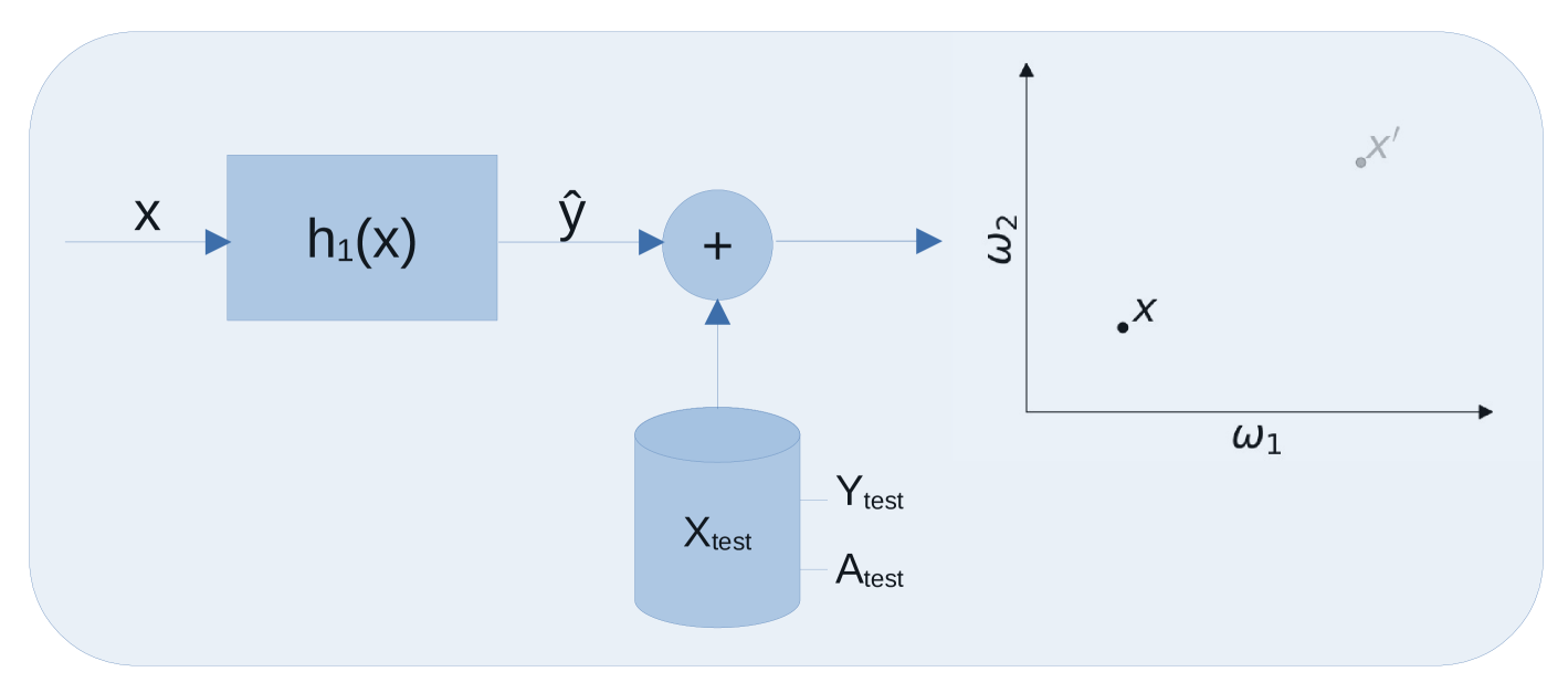
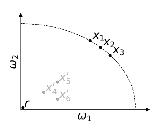
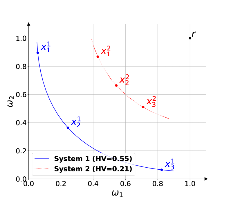
The first type of scenario considers a “black-box” ML system to provide binary outcomes for an input such that where . To measure the approximate Pareto solution , we assume the availability of a dataset that carries annotations for all considered objectives, i.e., the expected output of the classification , and demographic attributes . Fig. 1 contains a representation of this scenario in two optimization dimensions as and . As there is no tuning possibility to select the model (), this test evaluates the solution in the deployed ML system as it is provided.
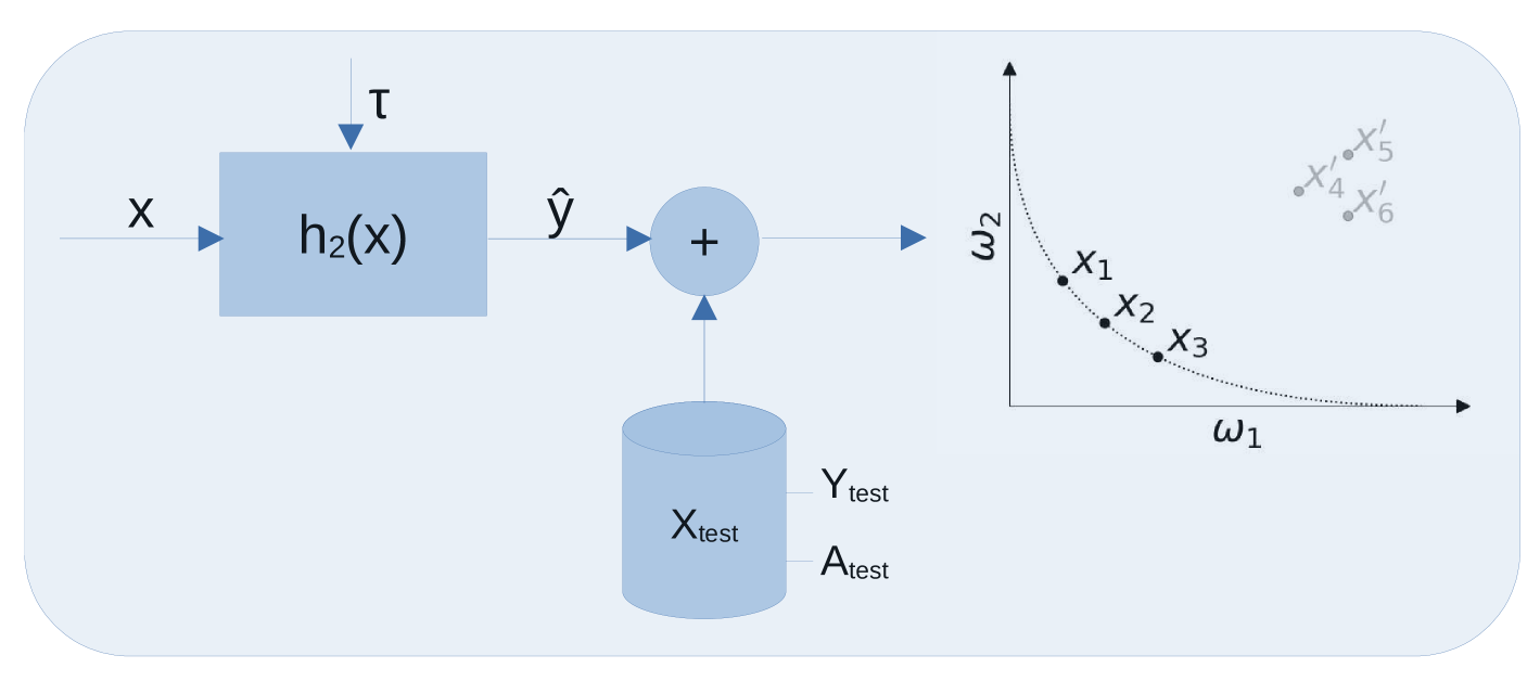
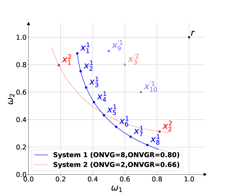
The second scenario defines the evaluation in a “white-box” manner for an ML system that is tunable over prediction scores (logits) as where . Model selection in may be achieved via so that a set of non-dominated solutions filtered by this parameter is available for performance assessment of the given ML system by using alongside and . This scenario is illustrated in Fig. 2 for two optimization dimensions, and .
In the following, we demonstrate each combination of these two scenarios in three assessment based use cases. We work with two synthetically generated approximate PF solutions, and , which represent different systems across the use cases, and evaluate them in a three dimensional setting to simulate an assessment in one direction as utility and two directions as fairness. Thus, we have an overall insight into the comparative trade-off performance of different ML systems by performing possible evaluation strategies commonly encountered during the assessment of ML systems.
III-A1 UC-1 - The comparative evaluation of two black-box systems
In this use-case, and are considered in a black-box manner as illustrated in Fig. 1 to assess their comparative performance using the proposed evaluation framework. Since both systems are assumed to be black-box, we only have the model for each as provided and assess the trade-off performance without any tuning.
III-A2 UC-2 - The comparative evaluation of one black-box system with one white-box system as a hybrid case
This is the use-case where the comparative performance of and is evaluated in a hybrid manner by applying black-box and white-box scenarios. is assumed to be deployed as it is without any tuning capability (black-box), and can be modified to have different settings based on user preference (white-box).
III-A3 UC-3 - The comparative evaluation of two white-box systems
This use-case considers the assessment of and as white-box by tuning them according to specified preferences. Thus, we demonstrate how the trade-off capacities of the systems can be assessed when tuning is feasible and how model selection is achieved by fully leveraging their capabilities.
We perform simulations for these use-cases in Section III-D to exemplify them quantitatively so that it is clarified how the proposed evaluation framework can be applied for such different assessment strategies given ML systems in comparison. These simulations are based on the synthetically generated systems, and , and exhibit the PF trend with non-dominated and dominated points as expected from the utility-fairness trade-off systems.
III-B MOO Based Performance Indicators
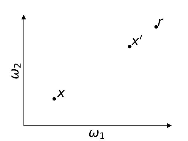
Central to MOO is the concept of the Pareto Front (PF), which delineates the set of all Pareto optimal solutions. A solution is deemed Pareto optimal if no other solution can enhance one objective without degrading another. In this regard, solutions residing on the PF are referred to as non-dominated solutions. More formally, given two points in the multidimensional solution space , the sample is said to dominate as , if is farther from the reference point than in any considered dimension of , and is strictly farther at least for one of them. We note , a.k.a. nadir point, represents the worst possible outcome for an experiment. In a minimization problem, for example, provides a smaller combined value for the target objective when compared to , see illustration in Fig. 3.

The Pareto optimal set is the set containing all the solutions that are non-dominated with respect to , defined as:
| (1) |
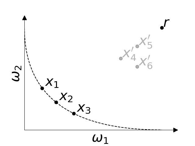
Pareto optimal solutions are called the Pareto set and the image of the Pareto set constructs the Pareto Front (PF) [37]. We note that, in real-world problems, the PF is rarely achievable. We refer to suboptimal solutions approximating the PF as [31] as shown in Fig. 4. We propose expanding on this approach for evaluating ML systems under multiple fairness constraints. This approach is analogous to the analysis of receiver operating characteristics (ROC) or detection-error trade-off curves in classical ML.
Whereas interpretation of a solution set considering two optimization dimensions is straightforward [16], concurrent analysis of multiple fairness constraints is typically done [14, 38] as a single degree of fairness by treating equity performances in isolation from one another. In this type of analysis, the dependency/correlation between different fairness criteria is not considered and the evaluation remains oversimplified. However, in a multi-task setting, every objective may conflict with each other, as one may not be improved without deteriorating others. This dependency between objectives, as is also the case for multiple fairness criteria alongside utility, should be projected into one shared space so that the multiple degrees of evaluation may be achieved in a fused way. To address this, we propose to characterize the solution set , representing an ML system using multiple criteria from MOO. These indicators will be assembled in an easy to interpret table and a plot. Qualitative analysis can still be carried out when the number of concurrently analyzed objectives is small () or when visual clutter is minimal in systems with . In all cases, the proposed evaluation framework via a PF characteristic remains usable.
III-B1 The Performance Indicators
In the design of metrics for MOO, four complementary performance criteria are typically considered to analyze the PF optimality: convergence, diversity, convergence-diversity, and capacity (or cardinality) [37, 39]. Measuring strict convergence, which denotes the proximity of the solution to the true PF, is not often attainable, we therefore focus on the other 3 properties, and describe them next.
Diversity
This indicator measures how well the non-dominated points are distributed or spread along the candidate solution set. Uniform Distribution (UD) and Overall Pareto Spread (OS) are some diversity measurements based on distribution and spread characteristics, respectively.
The UD indicator [32] evaluates the deviation characteristic of the non-dominated solution distribution and is formulated as:
| (2) |
where
| (3) |
and
| (4) |
is the niche radius that is problem dependent and can be adjusted based on the distribution of the candidate solution in the space. is the mean of the niche counts, , calculated as . The UD indicator is expected to be lower for a more uniform solution set. This indicator evaluates how uniform the solution set is spanned in the metric space based on an upper-bound distance, . For instance, a system with the lowest UD value among others exhibits the best performance as its solutions are the most uniformly distributed. Having a trade-off system with a lower UD value corresponds to a more uniformly spanned set of non-dominated points. This increases the likelihood of achieving a desired combination of utility with fairness in tuning, compared to a system with a higher UD. In this study, we apply a transformation to UD by taking its inverse as to make it consistent with other indicators so that a higher value means more uniformity. Although the UD measures the coverage of the solution space by the candidate set, it fails to characterize PF as any type of uniformly distributed solution (whether Pareto optimal or not) may yield high performance in terms of this indicator.
The OS indicator [30] assesses the spread of the solutions obtained by the trade-off system. For a minimization problem evaluated in different dimensions, this indicator is formulated as:
| (5) |
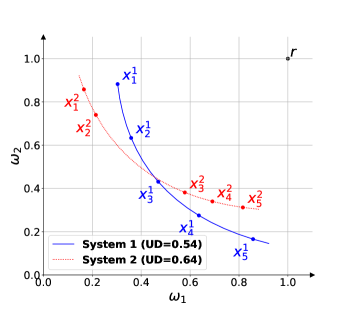
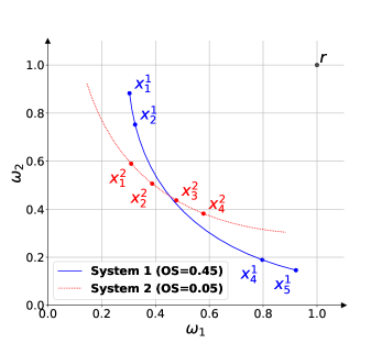
where the nominator and denominator are the absolute difference between the worst and best points for the candidate solution and Pareto optimal set , respectively. A higher OS value indicates a more widely spread solution. This indicator assesses how well the points from the candidate set spread towards the ideal of the optimal PF. For instance, a system with a higher OS score compared to others has more points close to the ideal point and fewer ones near the nadir (here, we can access the nadir and ideal points without having the exact PF solution, so there is no requirement to know the PF a priori). Having a higher OS value exhibits a more spread characteristic for non-dominated solutions, leading to an improvement in tuning performance for the trade-off system when the selection of models around the ideal point is expected. In this study, OS is in the range of and there is no transformation applied as it is scaled compatible with other indicators. Similarly to capacity and distribution, this measurement also fails to analyze Pareto optimality in a comprehensive manner as it only assesses the extreme cases without considering the entire PF space. In Fig. 5, both UD and OS indicators are exemplified in synthetically generated data. is said to have more uniformity and spread over as its points are more equally distributed, , (Fig. 5a) and it has more non-dominated points near the ideal, , (Fig. 5b).
Convergence-Diversity
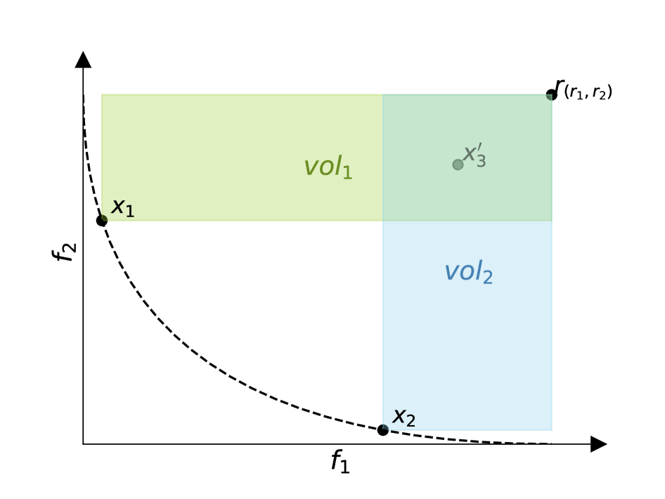
This measurement evaluates both convergence and diversity together so that the proximity (convergence) alongside the distribution/spread (diversity) of the candidate solution set are projected into a single scalar score. This unary metric measures the volume of the objective space covered by an approximation set, relying on a reference point for calculation. The HV takes distribution, spreading, and convergence into account at the same time, making it unique in this regard. Recognized for its distinctive properties, HV is Pareto-compliant, ensuring that any approximation set achieving maximum quality for a MOO contains all Pareto optimal solutions. The reference point can be simply attained by constructing a solution of worst objective function values. Given a minimization based MOO problem with two objectives, as shown in Fig. 6, it is expected to have solution sets with points that are in the best achievable state in the objective space. This should be the case even if the objectives are conflicting with each other. PF is one possible setting for such cases with non-dominated solutions. In Fig. 6, and are two non-dominated solutions drawn from the PF-like solution set (represented as a dashed curve) with one dominated solution, . The performance of such a solution set may be evaluated by the Hypervolume (HV) indicator to analyze how optimal the set is in terms of convergence and diversity. By discarding the dominated solution , which should not be part of an optimal solution set, the HV indicator is calculated as the union of two volumes constructed between each of the non-dominated solutions, and , and the reference point that is chosen as one of the poorly performing solutions in the space. The HV formulation is then as follows:
| (6) |
The formulation in (6) may be generalized as [40]:
| (7) |
In this study, HV is on the scale of as every solution in the metric space is represented by measurements between and . An illustrative example in Fig. 7 shows how two systems are evaluated in terms of HV. occupies a larger volume in 2D space compared to as it is further away from the reference point. HV reflects this situation with .
Capacity (or Cardinality)
This measurement quantifies the number of non-dominated points in the candidate solution set. The Overall Nondominated Vector Generation (ONVG) and Overall Nondominated Vector Generation Ratio (ONVGR) are some known capacity indicators. ONVG, proposed in [33], is the number of non-dominated solutions, , in the candidate solution set, , and formulated as:
| (8) |
As similarly proposed in [33], ONVGR is the ratio of the non-dominated solution cardinality against the cardinality of and it’s defined as:
| (9) |
Both ONVG and ONVGR yield higher scores for solution sets with greater capacity. These capacity-based indicators do not provide an extensive analysis like convergence or diversity do; they are only used as auxiliary indicators when other measurements are not discriminative. For instance, we can select a system with a higher ONVG over other systems when the convergence and diversity are the same for all. Furthermore, they may help analyze the effectiveness of the optimization, as a higher number of non-dominated points compared to dominated ones is a good indicator of how well the objective is approximated. Having a larger number of non-dominated points may also improve tuning the trade-off system as the possibility of finding an expected combination of utility alongside fairness would increase due to more optimal solutions in the objective space. Similarly to UD, we also apply a transformation just for ONVG by normalizing over the maximum value of it for the systems as to make it in the same range as others. On the other hand, ONVGR is in the range of with and indicating the absence of the non-dominated and dominated solutions, respectively. However, these measurements fail to capture PF optimality as the number of solutions does not provide information about the Pareto characteristic. Fig. 8 highlights that exhibits more capacity characteristic compared to in terms of ONVG and ONVGR as it has more non-dominated solutions, , and a bigger ratio on overall solutions, .
III-C Radar Chart: Compact Visualization
The assessment of a utility-fairness trade-off system with the aforementioned performance indicators can be reported as a measurement table. However, it’s also possible to convey this information in different ways such as the illustration in a chart summarizing all the performance indicators. A radar (spiderweb) chart is such a compact plot that compares different characteristics in the same projection and allows for easy comparative analysis of several systems over the same attributes.
The qualitative analysis resulting from the comparison of utility-fairness trade-offs with a radar chart makes it possible to select the optimal ML system showing more capacity, diversity, and convergence-diversity. This overall characteristic of the systems can also be quantified by calculating the areas occupied by each of them in the radar chart. The calculation of these areas allows for different systems to be comparable over very compact quantities compressed by the performance indicators in the table.
We consider the areas in the radar chart as polygons and use the Surveyor’s formula [41] for calculation. Given a polygon with ordered points as counterclockwise in the Cartesian coordinate system, , we define alongside . As we work in the Polar coordinate system to represent the systems in the radar chart, we define where is the radius and is the angle. In this stage, we need to convert the point in Polar coordinates to the counterpart in Cartesian one by and . After switching to the Cartesian coordinate system, we apply the Surveyor’s formula as shown below:
| (10) |
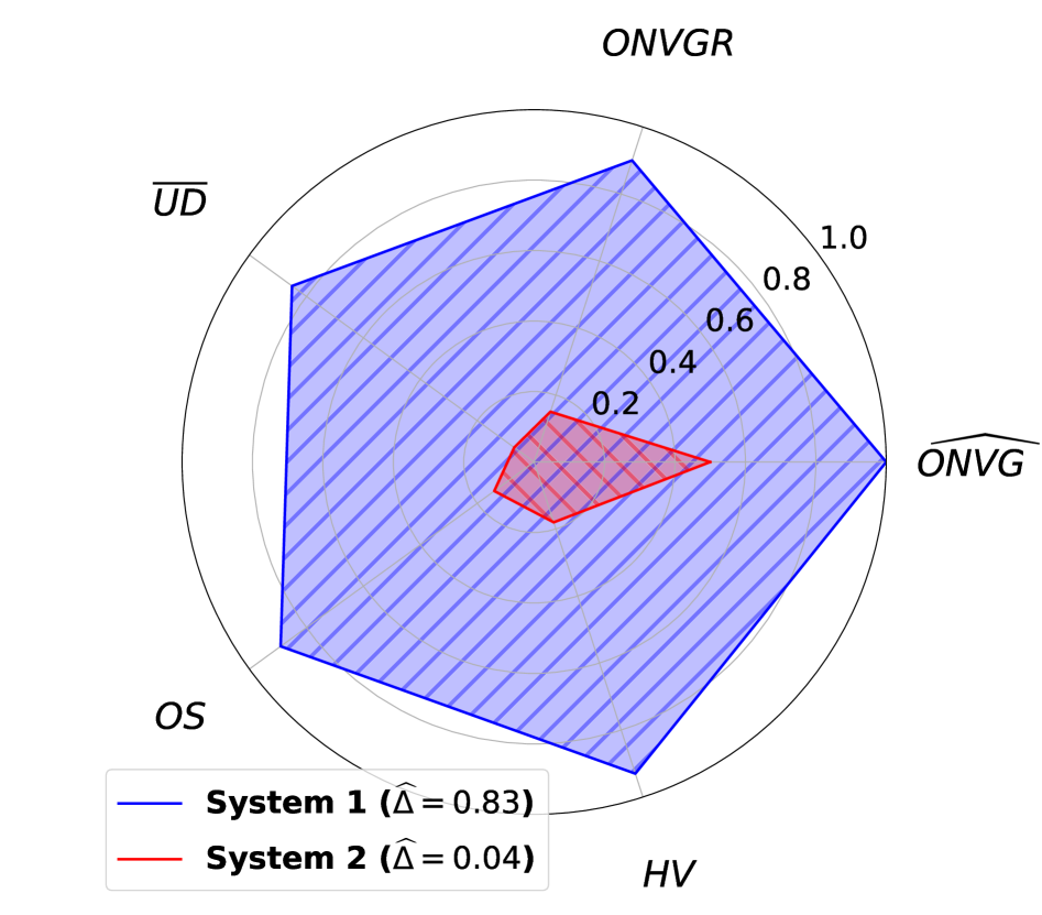
where is the determinant. The calculation of is then min-max normalized by to transform the area range to . Given a pentagon with 5 dimensions as shown in Fig. 9a, the theoretical lower and upper bounds of the area are and , respectively. This is analogous to the concept of the Area Under the Curve (AUC) over Receiver Operator Characteristic (ROC), so an area of is expected to be the best situation for a system. In the illustrative example of Fig. 9a, it can be easily seen from the radar chart that outperforms in every dimension. This can also be verified by their respective areas of and (Table 9b). We can also clearly observe that is closer to the ideal performance than , relying only on these areas.
| Convergence-Diversity | Capacity | Diversity | ||||
|---|---|---|---|---|---|---|
| Distribution | Spread | |||||
| System | ||||||
| 0.93 | 1.00 | 0.90 | 0.85 | 0.89 | 0.83 | |
| 0.18 | 0.50 | 0.15 | 0.07 | 0.14 | 0.04 | |
III-D Simulations for Use-cases
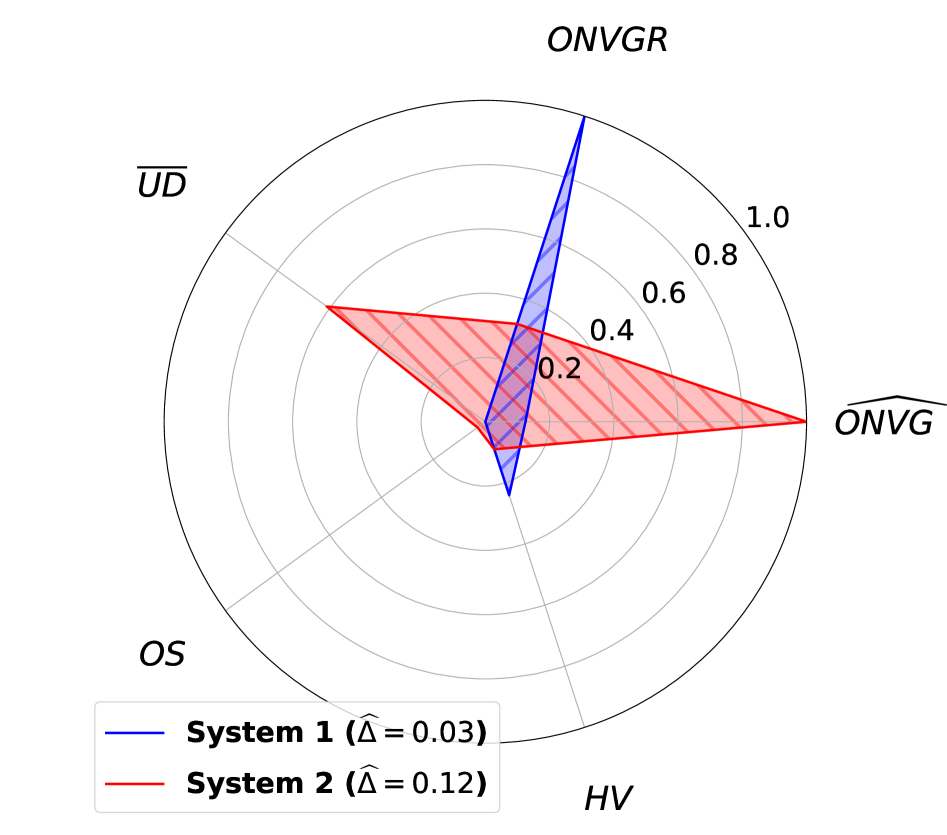
The first use-case, UC-1, focuses on black-box testing of and , corresponding to the first scenario (Fig. 1). As both systems have just non-dominated solution, they have the same and values of . In terms of the diversity measurements, it’s not possible then to evaluate both systems as there exist only one non-dominated solution. has a higher score than because its non-dominated solution is further away from the nadir point than the non-dominated solution of the other, resulting in a larger volume for . Table 10b and Fig. 10a show this comparison quantitatively and qualitatively. The radar chart in Fig. 10a illustrates the performance gap and HV dominance of over . The difference in the area is and it arises solely from the HV differences between the two systems. In this case, the proposed evaluation framework simplifies the comparison using a single indicator, HV, as the other indicators do not play a role in the model selection decision.
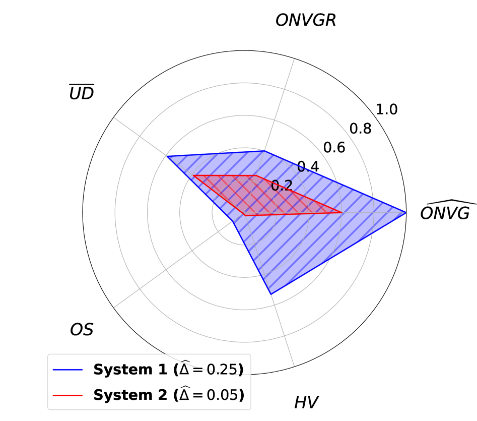
In the second use-case, UC-2, we perform hybrid testing with white (, Fig. 1) and black box cases (, Fig. 2). Eight different non-dominated solutions are considered out of , adjusting for against a single non-dominated solution for , as it is not tunable. Table 11b contains the indicator scores for both systems. outperforms for as it has more non-dominated solutions but results in a lower with a score of . Even though has distribution and spread indicators, they are not comparable since there is no score generated for . This can be observed in the radar chart shown in Fig. 11a. We can end up with a decision that outperforms overall, as seen in the difference of the areas .
| Convergence-Diversity | Capacity | Diversity | ||||
| Distribution | Spread | |||||
| System | ||||||
| 0.35 | 1.00 | 1.00 | - | 0 | 0.26 | |
| 0.03 | 1.00 | 1.00 | - | 0 | 0.20 | |
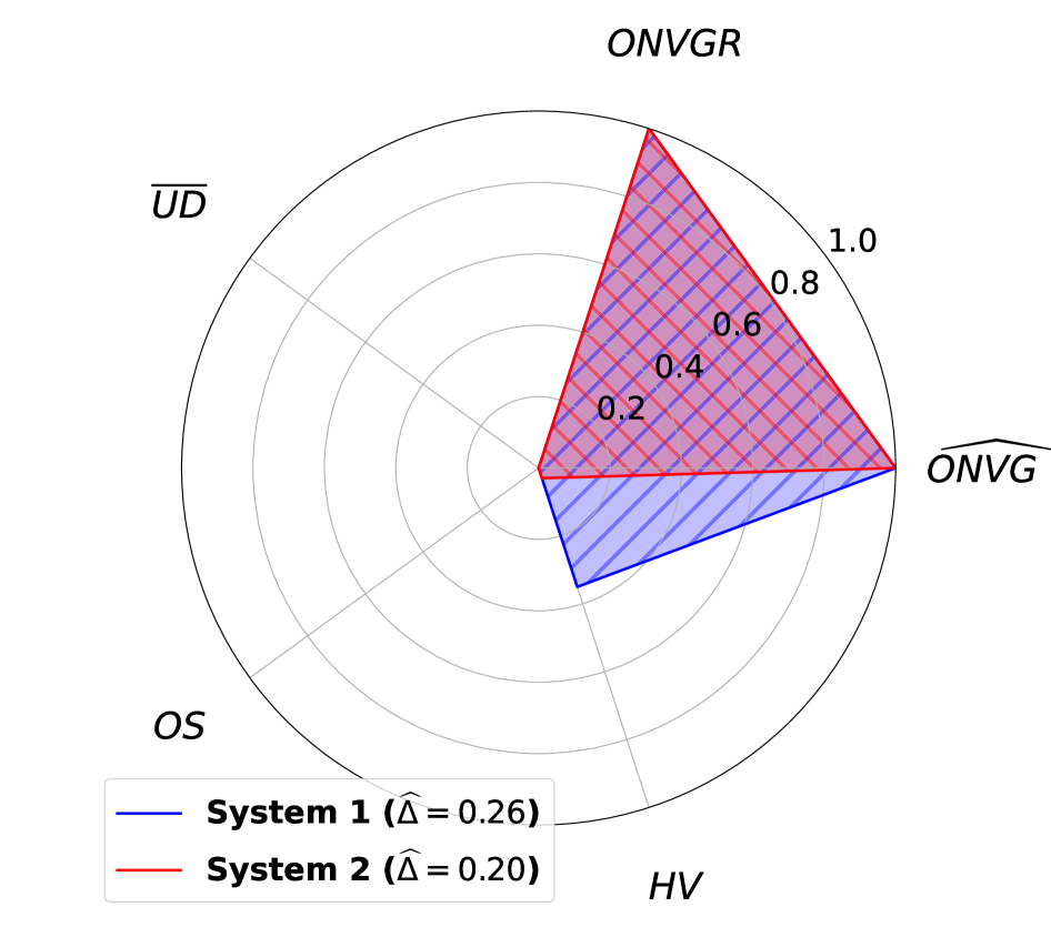
The last use-case, UC-3, considers white-box testing for both and , matching the second scenario (Fig. 2). and different non-dominated solutions were considered out of for and , respectively. As seen in Table 12b, outperforms in terms of , , , , and . This can also be interpreted through a visual inspection of the radar chart in Fig. 12a. Finally, the areas of both systems confirm this as well, .
We can derive some conclusions about performance indicators based on the observations regarding the use-cases above. Firstly, the black-box case only gives a partial characterization of the assessment since the ML system are not tunable. In this case, we obtain non-discriminative values for ONVG or ONVGR of 1.00 as seen in Fig. 10. Secondly, diversity is another issue when working with a low number of solutions. A system with only one solution does not allow us to evaluate UD and OS as there must be at least two solutions. For instance, UD is evaluated by measuring the distance between two solutions or OS is performed on the distance between the most/least optimal points from the system and the ideal/nadir points from the PF. A single point solution fails to have a score of UD and OS as seen in shown in Table 11b. Thirdly, HV may be the first decision point to select the system, which exhibits more PF characteristics, as it covers every aspect of convergence, diversity and capacity. There may be opposite cases between HV and the other indicators as seen in Fig. 12. A good indication of ONVG, ONVGR, UD, and OS does not work as well as evaluating the performance over HV, which has been proven to be a more reliable measurement for PF [37, 39].
| Convergence-Diversity | Capacity | Diversity | ||||
| Distribution | Spread | |||||
| System | ||||||
| 0.24 | 0.12 | 1.00 | - | 0 | 0.03 | |
| 0.09 | 1.00 | 0.32 | 0.61 | 3 | 0.12 | |
IV Empirical Validation
In this section, we demonstrate the effectiveness of the proposed evaluation framework empirically. A medical image dataset named the Harvard Glaucoma Fairness (HGF) containing a well-specified binary classification task and metadata with protected demographic attributes was used to showcase the novel evaluation framework in a realistic scenario [38]. The HGF dataset contains cases with a retinal nerve disease called glaucoma as well as samples of healthy patients [42]. Glaucoma is twice as common in Black patients when compared to other races, and more prevalent men [43, 38]. The dataset contains 2D retinal nerve fiber layer thickness (RNFLT) maps from three racial groups, namely Asian, Black and White, with a resolution of 200 200 pixels around the optic disk. The glaucoma/non-glaucoma ratio in the dataset is as . The prevalence of glaucoma in Asians, Blacks, and Whites in the HGF dataset is equibalanced as , and the gender distribution is as and for females and males, respectively. The ophthalmologic images from HGF are linked to sensitive attributes for race, gender, age, and ethnicity allowing the evaluation of the utility-fairness trade-off in proposed solutions.
To properly observe the full capabilities of the proposed method, we formulate the utility-fairness trade-off system as a bi-objective optimization problem. More specifically, we implement an ML solution for the demographically fair glaucoma classification using Pareto HyperNetworks (PHNs), which are tailored for Pareto optimality [40, 44]. A PHN is a Neural Network (NN) topology that is able to generate sub-NNs with varying degrees of compromise between multiple objectives. In our setting, each sub-NN corresponds to a different trade-off between utility and fairness, i.e., one sub-model represents a performance with higher utility and lower fairness, another has higher equity sacrificing from the classification accuracy. We construct the PHN topology based on the work from [40] and use ResNet-18 as the backbone alongside 25 different preference vectors that represent the sub-NNs with specific levels of utility and fairness. We optimize the utility and fairness by using weighted loss functions based on Binary Cross-Entropy (BCE) and Equalized Odds (EO), respectively, in a back-propagated manner.
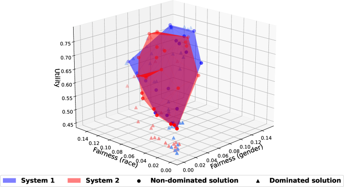
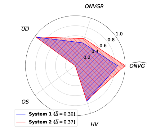
Fig. 13 summarizes the evaluation of both systems considering 3 metrics: classification accuracy (utility) alongside 2 equalized odds differences (EOD), one for race and another for gender. We follow the third analyzed scenario from Section III-A, since both systems can be evaluated through a white-box set up. Fig. 13a (a) highlights the importance of the proposed evaluation framework: even with only two fairness criteria considered besides utility, it is not possible to compare the two systems through visual inspection alone of this 3D plot. On the other hand, the proposed radar chart in Fig. 13b, helps to detect a slight advantage from when compared to . This can be further investigated by performing quantitative analysis in Table 13c. Although there is an inconsistency between HV and the other performance indicators (ONVG, ONVGR and UD), an area of over shows that is better-suited for the tuning of utility-fairness trade-offs than . In this case, it is not possible to differentiate the systems over OS as they both share an spread of . Finally, it is straightforward to interpret that both systems are far from optimality as they are below an ideal performance of .
| Convergence-Diversity | Capacity | Diversity | ||||
| Distribution | Spread | |||||
| System | ||||||
| 0.53 | 1.00 | 0.40 | 0.59 | 9 | 0.25 | |
| 0.02 | 0.60 | 0.24 | 0.39 | 1 | 0.05 | |
| Convergence-Diversity | Capacity | Diversity | ||||
|---|---|---|---|---|---|---|
| Distribution | Spread | |||||
| System | ||||||
| 0.75 | 0.84 | 0.48 | 0.97 | 0.30 | 0.30 | |
| 0.73 | 1.00 | 0.57 | 0.98 | 0.30 | 0.37 | |
V Discussion
This work presents the requirements and advantages of an evaluation framework assessing multidimensional utility-fairness trade-offs obtained with ML systems. The framework enhances the comparison of different modeling strategies, with the goal of selecting optimal solutions for real-world applications that require the assessment of multiple fairness criteria. The ease-of-use and effectiveness of the proposed framework are explored through comprehensive simulations and empirical studies using a medical image dataset designed to test fairness optimization approaches. Unlike previous evaluation frameworks, this work provides a series of steps for the selection process of ML systems in the context of multidimensional fairness exploring different criteria, supported by MOO principles. Characterizing the optimal PF is particularly useful in tasks where contradictory fairness performance indicators cannot be avoided, and trade-offs should be tuned to specific fairness requirements from decision-makers. Our framework could guide the tuning of ML systems to different notions of fairness for any sensitive attribute and metric in a simple and transparent manner.
As mentioned in Section II, the comprehensive analysis of PFs in multiple dimensions is a limitation of previously proposed fairness evaluation approaches. A summarized objective representation of performance indicators from the PFs, both as a radar chart and as a measurement table, overcomes the limitations from visualizing performance plots in multiple dimensions resulting from the assessment of different ML systems. Furthermore, analogous to AUC for ROC, our evaluation framework can transform the qualitative trend into a quantitative measurement, thus gathering all necessary information for the interpretation of the performance gap between the trade-off systems in consideration, and against an ideal solution.
There may be some limitations of the proposed evaluation framework. A restriction is the exponential cost for computing the MOO-based performance indicators as the number of objectives increases [37]. However, we argue that the majority of tasks studied in the literature focus on a small set of sensitive attributes, i.e., gender, age and race. The use of other performance indicators, such as Inverted Generational Distance [34], could be explored as alternative measurements to address this issue. Another issue to consider, is the equal weighting of all performance indicators, which normalizes the contribution of the different indicators in the final evaluation. This may not be desired in situations where an indicator can evaluate the systems in suboptimal performance and needs to have less impact on the final decision compared to others. The proposed evaluation framework could be extended to support the dynamic weighting of the indicators, so that the re-weighting can be performed based on the use-case. As a final limitation, there may also be situations in which the indicator measurements are the same or not feasible (refer OS and UD in Fig. 10, respectively) for all systems in comparison. In this case, such an indicator is useless to consider for the final decision and the proposed framework simplifies the evaluation to the joint contribution of the rest. This issue could be alleviated by using different indicators that discriminate more, as the proposed framework supports seamlessly including/excluding different types of indicators.
VI Conclusions
This paper proposes a multi-objective evaluation framework for utility-fairness trade-offs resulting from ML systems, using performance indicators based on MOO. The proposed framework is model and task agnostic, allowing for high flexibility in the comparison of ML strategies, even when they have been optimized for different objectives. This is an adaptive assessment framework that supports any kind of performance indicators, including the proposed method, for convergence, diversity and capacity analysis. The proposed framework is able to perform a comprehensive analysis of ML systems with a measurement table and radar chart, overcoming the limitations resulting from the qualitative assessment of solutions with multiple fairness requirements. These tools provide a structured and visual means to evaluate and compare multiple fairness metrics in machine learning systems. The measurement table allows for a clear, organized presentation of the data, while the radar chart offers a visual representation of how well the system performs across various fairness criteria. The effectiveness of the evaluation approach is verified by performing simulations and empirical analysis for a variety of use-cases, both with black and white box ML models. The proposed system is made available for public access to be applied in the context of multi-objective evaluation.
VII Acknowledgement
This work was supported by the Swiss National Science Foundation (SNSF) through the project FairMI - Machine Learning Fairness with Application to Medical Images under grant number 214653. We also thank Fundação de Amparo à Pesquisa do Estado de São Paulo (FAPESP), grants 21/14725-3 and 2023/12468-9.
References
- [1] V. Xinying Chen and J. N. Hooker, “A guide to formulating fairness in an optimization model,” Annals of Operations Research, vol. 326, no. 1, pp. 581–619, 2023.
- [2] D. Pessach and E. Shmueli, “A review on fairness in machine learning,” ACM Computing Surveys (CSUR), vol. 55, no. 3, pp. 1–44, 2022.
- [3] C. Starke, J. Baleis, B. Keller, and F. Marcinkowski, “Fairness perceptions of algorithmic decision-making: A systematic review of the empirical literature,” Big Data & Society, vol. 9, no. 2, p. 20539517221115189, 2022.
- [4] R. T. Rabonato and L. Berton, “A systematic review of fairness in machine learning,” AI and Ethics, pp. 1–12, 2024.
- [5] S. Barocas, M. Hardt, and A. Narayanan, Fairness and machine learning: Limitations and opportunities. MIT press, 2023.
- [6] A. Castelnovo, R. Crupi, G. Greco, D. Regoli, I. G. Penco, and A. C. Cosentini, “A clarification of the nuances in the fairness metrics landscape,” Scientific Reports, vol. 12, no. 1, p. 4209, 2022.
- [7] R. Dutt, O. Bohdal, S. Tsaftaris et al., “Fairtune: optimizing parameter efficient fine tuning for fairness in medical image analysis (2024).”
- [8] H. Zhao and G. J. Gordon, “Inherent tradeoffs in learning fair representations,” Journal of Machine Learning Research, vol. 23, no. 57, pp. 1–26, 2022.
- [9] S. Wei and M. Niethammer, “The fairness-accuracy pareto front,” Statistical Analysis and Data Mining: The ASA Data Science Journal, vol. 15, no. 3, pp. 287–302, 2022.
- [10] Z. Wang, K. Qinami, I. C. Karakozis, K. Genova, P. Nair, K. Hata, and O. Russakovsky, “Towards fairness in visual recognition: Effective strategies for bias mitigation,” in Proceedings of the IEEE/CVF conference on computer vision and pattern recognition, 2020, pp. 8919–8928.
- [11] Y. Yang, H. Zhang, J. W. Gichoya, D. Katabi, and M. Ghassemi, “The limits of fair medical imaging ai in real-world generalization,” Nature Medicine, pp. 1–11, 2024.
- [12] N. Akter, J. Fletcher, S. Perry, M. P. Simunovic, N. Briggs, and M. Roy, “Glaucoma diagnosis using multi-feature analysis and a deep learning technique,” Scientific Reports, vol. 12, no. 1, p. 8064, 2022.
- [13] Z. Lu, I. Whalen, Y. Dhebar, K. Deb, E. D. Goodman, W. Banzhaf, and V. N. Boddeti, “Multiobjective evolutionary design of deep convolutional neural networks for image classification,” IEEE Transactions on Evolutionary Computation, vol. 25, no. 2, pp. 277–291, 2020.
- [14] J. Buolamwini and T. Gebru, “Gender shades: Intersectional accuracy disparities in commercial gender classification,” in Conference on fairness, accountability and transparency. PMLR, 2018, pp. 77–91.
- [15] H. Gong and C. Guo, “Influence maximization considering fairness: A multi-objective optimization approach with prior knowledge,” Expert Systems with Applications, vol. 214, p. 119138, 2023.
- [16] C. Little, “To the fairness frontier and beyond: Identifying, quantifying, and optimizing the fairness-accuracy pareto frontier,” Master’s thesis, Rice University, 2023.
- [17] M. Hardt, E. Price, and N. Srebro, “Equality of opportunity in supervised learning,” Advances in neural information processing systems, vol. 29, 2016.
- [18] T. Jang and X. Wang, “Difficulty-based sampling for debiased contrastive representation learning,” in Proceedings of the IEEE/CVF Conference on Computer Vision and Pattern Recognition, 2023, pp. 24 039–24 048.
- [19] E. Z. Liu, B. Haghgoo, A. S. Chen, A. Raghunathan, P. W. Koh, S. Sagawa, P. Liang, and C. Finn, “Just train twice: Improving group robustness without training group information,” in International Conference on Machine Learning. PMLR, 2021, pp. 6781–6792.
- [20] P. Lahoti, A. Beutel, J. Chen, K. Lee, F. Prost, N. Thain, X. Wang, and E. Chi, “Fairness without demographics through adversarially reweighted learning,” Advances in neural information processing systems, vol. 33, pp. 728–740, 2020.
- [21] N. Jovanović, M. Balunovic, D. I. Dimitrov, and M. Vechev, “Fare: Provably fair representation learning with practical certificates,” in International Conference on Machine Learning. PMLR, 2023, pp. 15 401–15 420.
- [22] P. C. Roy and V. N. Boddeti, “Mitigating information leakage in image representations: A maximum entropy approach,” in Proceedings of the IEEE/CVF Conference on Computer Vision and Pattern Recognition, 2019, pp. 2586–2594.
- [23] J. S. Kim, J. Chen, and A. Talwalkar, “Fact: A diagnostic for group fairness trade-offs,” in International Conference on Machine Learning. PMLR, 2020, pp. 5264–5274.
- [24] T. Jang, P. Shi, and X. Wang, “Group-aware threshold adaptation for fair classification,” in Proceedings of the AAAI Conference on Artificial Intelligence, vol. 36, no. 6, 2022, pp. 6988–6995.
- [25] S. Liu and L. N. Vicente, “Accuracy and fairness trade-offs in machine learning: A stochastic multi-objective approach,” Computational Management Science, vol. 19, no. 3, pp. 513–537, 2022.
- [26] Y. Wang, X. Wang, A. Beutel, F. Prost, J. Chen, and E. H. Chi, “Understanding and improving fairness-accuracy trade-offs in multi-task learning,” in Proceedings of the 27th ACM SIGKDD Conference on Knowledge Discovery & Data Mining, 2021, pp. 1748–1757.
- [27] N. Jo, S. Aghaei, J. Benson, A. Gomez, and P. Vayanos, “Learning optimal fair decision trees: Trade-offs between interpretability, fairness, and accuracy,” in Proceedings of the 2023 AAAI/ACM Conference on AI, Ethics, and Society, 2023, pp. 181–192.
- [28] Q. Zhang, J. Liu, Z. Zhang, J. Wen, B. Mao, and X. Yao, “Fairer machine learning through multi-objective evolutionary learning,” in International conference on artificial neural networks. Springer, 2021, pp. 111–123.
- [29] K. Padh, D. Antognini, E. Lejal-Glaude, B. Faltings, and C. Musat, “Addressing fairness in classification with a model-agnostic multi-objective algorithm,” in Uncertainty in artificial intelligence. PMLR, 2021, pp. 600–609.
- [30] J. Wu and S. Azarm, “Metrics for quality assessment of a multiobjective design optimization solution set,” J. Mech. Des., vol. 123, no. 1, pp. 18–25, 2001.
- [31] E. Zitzler, L. Thiele, M. Laumanns, C. M. Fonseca, and V. G. Da Fonseca, “Performance assessment of multiobjective optimizers: An analysis and review,” IEEE Transactions on evolutionary computation, vol. 7, no. 2, pp. 117–132, 2003.
- [32] K. C. Tan, T. H. Lee, and E. F. Khor, “Evolutionary algorithms for multi-objective optimization: Performance assessments and comparisons,” Artificial intelligence review, vol. 17, no. 4, pp. 251–290, 2002.
- [33] D. A. Van Veldhuizen and G. B. Lamont, “On measuring multiobjective evolutionary algorithm performance,” in Proceedings of the 2000 congress on evolutionary computation. CEC00 (Cat. No. 00TH8512), vol. 1. IEEE, 2000, pp. 204–211.
- [34] C. A. Coello Coello and M. Reyes Sierra, “A study of the parallelization of a coevolutionary multi-objective evolutionary algorithm,” in MICAI 2004: Advances in Artificial Intelligence: Third Mexican International Conference on Artificial Intelligence, Mexico City, Mexico, April 26-30, 2004. Proceedings 3. Springer, 2004, pp. 688–697.
- [35] D. Zietlow, M. Lohaus, G. Balakrishnan, M. Kleindessner, F. Locatello, B. Schölkopf, and C. Russell, “Leveling down in computer vision: Pareto inefficiencies in fair deep classifiers,” in Proceedings of the IEEE/CVF Conference on Computer Vision and Pattern Recognition, 2022, pp. 10 410–10 421.
- [36] Z. Yang, Y. L. Ko, K. R. Varshney, and Y. Ying, “Minimax auc fairness: Efficient algorithm with provable convergence,” in Proceedings of the AAAI Conference on Artificial Intelligence, vol. 37, no. 10, 2023, pp. 11 909–11 917.
- [37] C. Audet, J. Bigeon, D. Cartier, S. Le Digabel, and L. Salomon, “Performance indicators in multiobjective optimization,” European journal of operational research, vol. 292, no. 2, pp. 397–422, 2021.
- [38] Y. Luo, Y. Tian, M. Shi, L. R. Pasquale, L. Q. Shen, N. Zebardast, T. Elze, and M. Wang, “Harvard glaucoma fairness: a retinal nerve disease dataset for fairness learning and fair identity normalization,” IEEE Transactions on Medical Imaging, 2024.
- [39] S. Jiang, Y.-S. Ong, J. Zhang, and L. Feng, “Consistencies and contradictions of performance metrics in multiobjective optimization,” IEEE transactions on cybernetics, vol. 44, no. 12, pp. 2391–2404, 2014.
- [40] A. Navon, A. Shamsian, G. Chechik, and E. Fetaya, “Learning the pareto front with hypernetworks,” arXiv preprint arXiv:2010.04104, 2020.
- [41] B. Braden, “The surveyor’s area formula,” The College Mathematics Journal, vol. 17, no. 4, pp. 326–337, 1986.
- [42] Y.-C. Tham, X. Li, T. Y. Wong, H. A. Quigley, T. Aung, and C.-Y. Cheng, “Global prevalence of glaucoma and projections of glaucoma burden through 2040: a systematic review and meta-analysis,” Ophthalmology, vol. 121, no. 11, pp. 2081–2090, 2014.
- [43] N. Khachatryan, M. Pistilli, M. G. Maguire, R. J. Salowe, R. M. Fertig, T. Moore, H. V. Gudiseva, V. R. Chavali, D. W. Collins, E. Daniel et al., “Primary open-angle african american glaucoma genetics (poaagg) study: Gender and risk of poag in african americans,” PloS one, vol. 14, no. 8, p. e0218804, 2019.
- [44] D. Ha, A. Dai, and Q. V. Le, “Hypernetworks,” arXiv preprint arXiv:1609.09106, 2016.