Computing Certificates of Strictly Positive Polynomials in Archimedean Quadratic Modules

Abstract

New results on computing certificates of strictly positive polynomials in Archimedean quadratic modules are presented. The results build upon (i) Averkov’s method for generating a strictly positive polynomial for which a membership certificate can be more easily computed than the input polynomial whose certificate is being sought, and (ii) Lasserre’s method for generating a certificate by successively approximating a nonnegative polynomial by sums of squares. First, a fully constructive method based on Averkov’s result is given by providing details about the parameters; further, his result is extended to work on arbitrary subsets, in particular, the whole Euclidean space $\mathbb{R}^{n}$, producing globally strictly positive polynomials. Second, Lasserre’s method is integrated with the extended Averkov construction to generate certificates. Third, the methods have been implemented and their effectiveness is illustrated. Examples are given on which the existing software package RealCertify appears to struggle, whereas the proposed method succeeds in generating certificates. Several situations are identified where an Archimedean polynomial does not have to be explicitly included in a set of generators of an Archimedean quadratic module. Unlike other approaches for addressing the problem of computing certificates, the methods/approach presented is easier to understand as well as implement.

Key words: Quadratic module, certificate, sum of squares, Positivstellensatz

1 Introduction

Consider a polynomial set $G=\{g_{1},\ldots,g_{s}\}$ in the multivariate polynomial ring $\mathbb{R}[\bm{x}]$. The quadratic module generated by $G$ is $\operatorname{QM}(G)=\{\sigma_{0}+\sum_{i=1}^{s}\sigma_{i}\cdot g_{i}\,|\,\sigma_{i}\mbox{ is a sum of squares in }\mathbb{R}[\bm{x}]\mbox{ for }i\!=\!0,\ldots,s\}$ [10, 12]. Quadratic modules are fundamental objects in real algebraic geometry and are heavily related to Hilbert’s 17th problem [5] and Positivstellensatz. This paper addresses the problem of computing certificates that witness the membership of polynomials in quadratic modules in $\mathbb{R}[\bm{x}]$. The certificates here are also referred to as sum-of-squares representations in the literature. In particular, we present new results and constructive methods to compute the sum-of-squares multipliers, or certificates, of strictly positive polynomials in Archimedean finitely generated quadratic modules.

Several contributions in the field identify conditions whenever representations in preorderings and quadratic modules exist. Noteworthy are the seminal results by Schmüdgen [16] and Putinar’s Positivstellensatz [15] for strictly positive polynomials over compact semialgebraic sets. However, the above-mentioned results about membership problems do not produce certificates as their proofs are non-constructive. In the case of Hilbert’s 17th problem, as an example, for a given non-negative polynomial $p$ it is nontrivial to generate a certificate consisting of rational functions $\frac{a_{i}}{b_{i}}$’s such that $p=\sum_{i}\left({\frac{a_{i}}{b_{i}}}\right)^{2}$. A solution to the certificate problem for Archimedean preorderings is discussed in [17, 18] which is constructive by including an Archimedean polynomial in the set of generators; an algorithm is described using Gröbner basis techniques to lift positivity conditions to a simplex and using Pólya bounds [14] to compute certificates.

Contributions. This paper presents new results about computing certificates of strictly positive polynomials in Archimedean quadratic modules. The results build upon (i) Averkov’s method [1] for generating a strictly positive polynomial for which a membership certificate can be more easily computed than the input polynomial whose certificate is being sought, and (ii) Lasserre’s method [6] for generating a certificate by successively approximating a non-negative polynomial by sums of squares.

A fully constructive method based on Averkov’s result in [1] is given by providing details about the parameters left out there. Further, his result is extended to work on non-compact subsets, in particular, producing globally strictly positive polynomials on $\mathbb{R}^{n}$ (compare Theorem 3.3 and Lemma 2.3 for the details). This is discussed in Section 3. Then in Section 4 we extend Lasserre’s method to reduce any globally strictly positive polynomial by a single polynomial to a sum of squares. These two extensions of Averkov’s construction and Lasserre’s method are proved in a constructive manner and they serve as the theoretical and algorithmic foundations of our method for solving the certificate problem.

To apply extended Averkov’s construction to the certificate problem, there are two technical problems to solve: construction of a polynomial in the quadratic module with a bounded non-negative set and a polynomial with a global lower bound. The former problem is easy when some generator of the quadratic module has a bounded non-negative set, otherwise we explicitly show how to construct such a polynomial in the univariate case and use an Archimedean polynomial in the multivariate case. Unlike the methods in the literature which depend on the inclusion of Archimedean polynomials in the generating sets, here we identify the situations where we can avoid inclusion of Archimedean polynomials and thus in these situations the certificates computed by our method are with respect to the original generators of the quadratic modules without the Archimedean polynomials.

After providing solutions to these two technical problems, in Section 5 we propose the algorithm (Algorithm 4) for computing certificates of strictly positive polynomials in Archimedean quadratic modules by using the extended Averkov’s construction and Lasserre’s method. Unlike other approaches for addressing the problem of computing certificates, the proposed algorithm is easier to understand as well as implement.

All the methods discussed in the paper have been implemented and their effectiveness is illustrated. Examples are given on which RealCertify, a software package for solving the certificate problem based on semidefinite programming [8], appears to struggle, whereas the proposed method succeeds in generating certificates. Several examples are given where an Archimedean polynomial does not have to be explicitly included in a given set of generators of an Archimedean quadratic module.

Related work. Among the literature most related to the topic of the paper, the following two publications stand out. In [9], the authors use the extended Gram matrix method to obtain an approximate certificate of the input polynomial in a quadratic module and a refinement step to compute sums of squares to represent the difference of the input polynomial and the approximate certificate (or the ”error term”). The method requires the polynomial set of generators to include an Archimedean polynomial as part of the assumptions. The authors also discuss time complexity for the termination of their algorithm and bounds of the degrees and bit size complexity of the coefficients in the certificates obtained; bounds of the degrees of the certificates rely on the complexity analysis discussed in [11]. Their implementation, RealCertify [8], relies on numerical methods, making them ineffective in certain situations. The performance of the approach proposed in the paper is compared with that of RealCertify later in Section 6.

More recently, [2] provides degree bounds on the sum-of-square multipliers in the certificate problem for a strictly positive polynomial $f$ in an Archimedean quadratic module $\operatorname{QM}(G)$. This is done in two steps. First, a new polynomial $h\in\operatorname{QM}(G)$ is constructed such that $f-h$ is strictly positive over the hypercube $\left[-1,1\right]^{n}$ by using a modified construction to Averkov’s result [1, Lemma 3.3]. Secondly, the construction in [7] is used to obtain a certificate of $f-h$ in the preordering generated by $1-\sum_{i=1}^{n}{x_{i}^{2}}$ that equals $\operatorname{QM}(1-\sum_{i=1}^{n}{x_{i}^{2}})$. This step relies on the Jackson kernel method, which seems highly complex and also difficult to algorithmize. Rearranging the previous results, the authors find a certificate of $f$ in $\operatorname{QM}(G\cup\{1-\sum_{i=1}^{n}{x_{i}^{2}}\})$. This approach also relies on adding an Archimedean polynomial to the generators. The authors do not report any implementation of their approach.

Because of their dependence on requiring an Archimedean polynomial as one of the generators, both of these papers are unable to compute certificates in case the generators of an Archimedean quadratic module do not explicitly include an Archimedean polynomial.

2 Preliminaries

2.1 Quadratic modules in $\mathbb{R}[x_{1},\ldots,x_{n}]$

Consider the multivariate polynomial ring $\mathbb{R}[x_{1},\ldots,x_{n}]$ over the field $\mathbb{R}$ of real numbers. We denote $\bm{x}=(x_{1},\ldots,x_{n})$, $\mathbb{R}[\bm{x}]=\mathbb{R}[x_{1},\ldots,x_{n}]$, and $\|\bm{x}\|=\sqrt{x_{1}^{2}+\cdots+x_{n}^{2}}$. For any $\bm{\alpha}=(a_{1},\ldots,a_{n})\in\mathbb{N}^{n}$, denote $\bm{x}^{\bm{\alpha}}=x_{1}^{a_{1}}\cdots x_{n}^{a_{n}}$.

A polynomial in $\mathbb{R}[\bm{x}]$ is called a sum of squares if it can be expressed as a sum of squares of polynomials in $\mathbb{R}[\bm{x}]$. We denote the set of all sums of squares in $\mathbb{R}[\bm{x}]$ by $\sum\mathbb{R}[\bm{x}]^{2}$. Any sum of squares in $\mathbb{R}[\bm{x}]$ is a polynomial of even total degree and is non-negative over $\mathbb{R}^{n}$.

Definition 2.1.

A polynomial set $M\subseteq\mathbb{R}[\bm{x}]$ is called a quadratic module in $\mathbb{R}[\bm{x}]$ if $M$ is closed under addition, $1\in M$, and for any $f\in\mathbb{R}[\bm{x}]$ and $m\in M$, $f^{2}m\in\mathbb{R}[\bm{x}]$. A quadratic module $M$ in $\mathbb{R}[\bm{x}]$ is finitely generated if there exists a finite set $G=\{g_{1},\dots,g_{s}\}\subseteq\mathbb{R}[\bm{x}]$ such that $M=\{\sigma_{0}+\sum_{i=1}^{s}\sigma_{i}g_{i}\,|\,\sigma_{i}\in\sum\mathbb{R}[\bm{x}]^{2},i\!=\!0,\ldots,s\}$. In this case, $M$ is said to be generated by $G$ and written as $M=\operatorname{QM}(G)$.

Let $G$ be a polynomial set in $\mathbb{R}[\bm{x}]$. Then the non-negative set of $G$, denoted by $\operatorname{S}(G)$, is defined to be $\{\bar{\bm{x}}\in\mathbb{R}^{n}\,|\,g_{i}(\bar{\bm{x}})\geq 0,i=1,\ldots,s\}$. A finitely generated quadratic module $\operatorname{QM}(G)$ in $\mathbb{R}[\bm{x}]$ is said to be bounded if the non-negative set $\operatorname{S}(G)$ is a bounded set in $\mathbb{R}^{n}$ and unbounded otherwise. Furthermore, a quadratic module in $\mathbb{R}[\bm{x}]$ is said to be Archimedean if it contains the polynomial $N-\sum_{i=1}^{n}x_{i}^{2}$ for some $N\in\mathbb{N}$, which is called Archimedean polynomial. It is clear that Archimedean quadratic modules are bounded.

Given a quadratic module $\operatorname{QM}(G)$ in $\mathbb{R}[\bm{x}]$, the fundamental membership problem is to determine whether an arbitrary polynomial $f$ belongs to $\operatorname{QM}(G)$, and this problem has been solved in specific cases. The well-known Putinar’s Positivstellensatz about strictly positive polynomials is recalled below.

Theorem 2.2 (Putinar Positivstellensatz, [15]).

Let $G=\{g_{1},\ldots$ $,g_{s}\}$ be a polynomial set in $\mathbb{R}[\bm{x}]$ such that $\operatorname{QM}(G)$ is Archimedean and $f\in\mathbb{R}[\bm{x}]$ be a polynomial that is strictly positive on $\operatorname{S}(G)$. Then $f\in\operatorname{QM}(G)$.

2.2 Averkov’s Lemma to aid computing certificates of Positivstellensatz theorems

Several (semi)constructive approaches exist in the literature to compute certificates of strictly positive polynomials in quadratic modules [19, 11, 1]. A common step in these approaches is the perturbation of the input polynomial $f\in\operatorname{QM}(G)$ by translating the positivity of $f$ over $\operatorname{S}(G)$ to the positivity of $f-h$ in some compact set $B$ where $h\in\operatorname{QM}(G)$. The following result due to Averkov is used in our construction. For self-containedness, the proof in [1] is sketched without giving details of the derivation.

Lemma 2.3 ([1, Lemma 3.3]).

Let $G=\{g_{1},\ldots,g_{s}\}$ be a polynomial set in $\mathbb{R}[\bm{x}]$ and $f$ be a polynomial in $\mathbb{R}[\bm{x}]$ such that $f>0$ on $\operatorname{S}(G)$. Then, for any compact subset $B$ of $\mathbb{R}^{n}$, a polynomial $h\in\operatorname{QM}(G)$ exists such that $f-h>0$ on $B$.

Proof.

Let $T=\{\bar{\bm{x}}\in B\leavevmode\nobreak\ |\leavevmode\nobreak\ f(\bar{\bm{x}})<0\}$. We use $a$ as the function $\bm{x}\mapsto(g_{1}(\bm{x}),\ldots,g_{s}(\bm{x}))$ from $\mathbb{R}^{n}$ to $\mathbb{R}^{s}$. Since $a(B)$ is compact, there exists $\gamma>0$ such that $a(B)\subseteq(-\infty,2\gamma]^{s}$. By the assumption on $f$, $a(T)\cap[0,2\gamma]^{s}=\emptyset$. As $a(T)$ and $[0,2\gamma]^{s}$ are compact, there exists $\epsilon>0$ such that $a(T)\cap[-2\epsilon,\gamma]^{s}=\emptyset$. Thus, if $\bar{\bm{x}}\in B$ and $g_{i}(\bar{\bm{x}})\geq-2\epsilon$ for each $i=1,\dots,s$, then $f(\bar{\bm{x}})>0$. Consequently, $\mu:=\min\{f(\bar{\bm{x}})\leavevmode\nobreak\ |\leavevmode\nobreak\ \bar{\bm{x}}\in B\ \mbox{and}\ g_{i}(\bar{\bm{x}})\geq-2\epsilon\mbox{ for }i=1,\ldots,s\}>0$.

Consider the polynomial

$$h=\sum_{i=1}^{s}g_{i}\left(\frac{g_{i}-\gamma}{\gamma+\epsilon}\right)^{2N}$$ (1)

and denote

$$c(N):=2\gamma\left(\frac{\gamma}{\gamma+\epsilon}\right)^{2N},\quad C(N):=2\epsilon\left(\frac{\gamma+2\epsilon}{\gamma+\epsilon}\right)^{2N}.$$

For $\bar{\bm{x}}\in B$, if $g_{i}(\bar{\bm{x}})\geq-2\epsilon$ for each $i=1\ldots,s$, we have $f(\bar{\bm{x}})-h(\bar{\bm{x}})\geq\mu-sc(N)$; otherwise if $g_{i}(\bar{\bm{x}})<-2\epsilon$ for some $i\leavevmode\nobreak\ (1\leq i\leq s)$, we have $f(\bar{\bm{x}})-h(\bar{\bm{x}})\geq\min_{y\in B}f(y)-sc(N)+C(N)$. Since $c(N)\rightarrow 0$ and $C(N)\rightarrow+\infty$ as $N\rightarrow+\infty$, by choosing $N$ sufficiently large, we deduce $f(\bar{\bm{x}})-h(\bar{\bm{x}})>0$ for every $\bar{\bm{x}}\in B$. ∎

3 Extending Averkov’s results

This section discusses two extensions to Averkov’s lemma. Firstly, details about deriving various parameters are given. Secondly, the lemma is generalized to allow arbitrary subsets of $\mathbb{R}^{n}$ for $B$, thus relaxing the requirement that $B$ be compact, as well as making the generalized lemma more useful in wider contexts.

3.1 Estimation of parameters $\epsilon$, $\gamma$, and $N$

The original proof for Lemma 2.3 is semi-constructive: a specific polynomial $h$ in (1) is constructed and proved to satisfy the conditions of the lemma; however, parameters like $\epsilon,\gamma$ and $N$ are existentially introduced without specifying proper values. We provide details on the computation of the values of these parameters in the proposition below so that with these values, the constructed polynomial $h$ in (1) satisfies the conditions of the lemma.

Proposition 3.1.

þ Let $g_{1},\ldots,g_{s},f$, and $B$ be as stated in Lemma 2.3 and the parameters $\gamma$, $\epsilon$, and $N$ be such that

$$\begin{split}\gamma&=\frac{1}{2}\max_{1\leq i\leq s}\{\max g_{i}(\bm{x})\leavevmode\nobreak\ |\leavevmode\nobreak\ \bm{x}\in B\},\\ \epsilon&<\frac{1}{2}\left|\max_{\bm{x}}\{\min_{1\leq i\leq s}g_{i}(\bm{x})\leavevmode\nobreak\ |\leavevmode\nobreak\ \bm{x}\in f^{-1}((-\infty,0))\cap B\}\right|,\\ N&>\frac{1}{2}\max\left\{\frac{\log(\mu)-\log(2s\gamma)}{\log(\gamma)-\log(\gamma+\epsilon)},\frac{\log(M+\mu)-\log(2\epsilon)}{\log(\gamma+2\epsilon)-\log(\gamma+\epsilon)}\right\},\end{split}$$ (2)

where $M=-\min_{\bm{y}\in B}f(\bm{y})$. Then the polynomial $h$ in (1) satisfies $f-h>0$ on $B$.

Proof.

From the proof of Lemma 2.3, one can see that $\gamma$ needs to satisfy the condition that $2\gamma\geq g_{i}(\bar{\bm{x}})$ for each $i=1,\ldots,s$ and any $\bar{\bm{x}}\in B$, and thus the value of $\gamma$ in (2) suffices.

The condition for $\epsilon$ is that $a(T)\cap[-2\epsilon,2\gamma]^{s}=\emptyset$. Then we claim that for any $\bar{\bm{x}}\in T$, there exists $g_{i}\leavevmode\nobreak\ (1\leq i\leq s)$ such that $g_{i}(\bar{\bm{x}})<-2\epsilon$. Otherwise, assume that there exists $\bar{\bm{x}}\in T$ such that $g_{i}(\bar{\bm{x}})\geq-2\epsilon$ for $i=1,\ldots,s$, then we have $(g_{1}(\bar{\bm{x}}),\ldots,g_{s}(\bar{\bm{x}}))\in a(T)\cap[-2\epsilon,2\gamma]^{s}$: a contradiction. From this we know that $-2\epsilon>\min_{i=1,\ldots,s}g_{i}(\bm{x})$ for all $\bm{x}\in T$, and thus the value of $\epsilon$ in (2) suffices.

In the end, we prove the inequality for $N$. Let $M=-\min_{\bm{y}\in B}f({\bm{y}})$. Then from the proof of Lemma 2.3, one can see that if both $\mu-sc(N)$ and $M-sc(N)+C(N)$ are positive, then $f-h$ is also positive. From $\mu-sc(N)>0$, it follows that $c(N)=2\gamma\left(\frac{\gamma}{\gamma+\epsilon}\right)^{2N}\!<\!\frac{\mu}{s}$. Therefore, we can set $2N>\frac{\log(\mu)-\log(2s\gamma)}{\log(\gamma)-\log(\gamma+\epsilon)}$. Then with $c(N)<\frac{\mu}{m}$, we can set $C(N)>M+\mu$ so that $-M-sc(N)+M+\mu>0$. From this constraint, we obtain the following inequality for $N$: $2N>\frac{\log(M+\mu)-\log(2\epsilon)}{\log(\gamma+2\epsilon)-\log(\gamma+\epsilon)}$. Taking the maximum of both values in the right hands of the two inequalities above, we have the value for $N$ in (2). ∎

Plugging the detailed values of the parameters in Proposition 3.3 into Averkov’s method (Lemma 2.3), Algorithm 1 below is derived, making Averkov’s result constructive.

Input: A polynomial set $G=\{g_{1},\dots,g_{s}\}\subseteq\mathbb{R}[\bm{x}]$, a polynomial $f\in\mathbb{R}[\bm{x}]$ such that $f>0$ over $\operatorname{S}(G)$, and a compact set $B\subseteq\mathbb{R}^{n}$

Output: A sequence of sum-of-squares multipliers $(\sigma_{1},\ldots,\sigma_{s})$ in $\mathbb{R}[\bm{x}]$ such that $f-\sum_{i=1}^{s}{\sigma_{i}g_{i}}>0$ over $B$

3

4$M:=\min_{\bm{y}\in B}f(\bm{y})$;

5

6if $M>0$ then

7    return $(0,0,\ldots,0)$;

8   

9 else

10    Choose $\gamma$, $\epsilon$, and $N$ as in (2);

11    return $\left(\left(\frac{g_{1}-\gamma}{\gamma+\epsilon}\right)^{2N},\ldots,\left(\frac{g_{s}-\gamma}{\gamma+\epsilon}\right)^{2N}\right)$;

12   

$\texttt{certificate}:=\operatorname{\sf Averkov}(G,f,B)$

Algorithm 1 Algorithm for Averkov’s construction

$\texttt{certificate}:=\operatorname{\sf Averkov}(G,f,B)$

Example 3.2.

We illustrate Algorithm 1 with the polynomial set $G=\{g_{1},g_{2},g_{3}\}\subset\mathbb{R}[x]$, where $g_{1}=(x+4)(x+1)(x-1)(x-4)$, $g_{2}=x+3$, and $g_{3}=-(x-3)$, and a polynomial $f=-(x+2)(x-2)$ which is positive on $\operatorname{S}(G)=[-1,1]$. Consider the compact set $B=[-5,5]$. First, we compute the minimum of $f$ over $B$, which is $M=-21$. Since it is not positive, we follow the else block in the algorithm. The values of $\epsilon$, $\gamma$, and $N$ computed with (2) are $0.446261$, $2.94026$, and $655$ respectively. One can check that the polynomial $f-\sum_{i=1}^{3}{\sigma_{i}g_{i}}$ is positive over $B$ with the returned certificates $\sigma_{i}=\left(\frac{g_{i}-\gamma}{\gamma+\epsilon}\right)^{2N}$ for $i=1,\dots,3$.

3.2 Generalization of Averkov’s Lemma

This subsection discusses how Averkov’s lemma 2.3 can be extended by generalizing the compact set $B$ to any subset in $\mathbb{R}^{n}$ when the set $G$ has a single generator. Using this result, by setting $B=\mathbb{R}$ in the univariate case, the requirement to add an Archimedean polynomial (whose certificates cannot be easily computed) to the set of generators can be relaxed, thus allowing the computation of the certificates directly with respect to the original generators $G$.

Theorem 3.3.

Let $g\in\mathbb{R}[\bm{x}]$ be a polynomial with bounded $\operatorname{S}(g)$ and $f\in\mathbb{R}[\bm{x}]$ be strictly positive on $\operatorname{S}(g)$. Then, for any subset $B$ of $\mathbb{R}^{n}$, there exists a polynomial $h\in\operatorname{QM}(g)$ such that $f-h>0$ over B.

Proof.

Choose $M>0$ such that $\operatorname{S}(g)\cap\{\bm{x}\in\mathbb{R}^{n}\leavevmode\nobreak\ |\leavevmode\nobreak\ \|\bm{x}\|\geq M\}=\emptyset$. This is always possible because $\operatorname{S}(g)$ is bounded. Let $K=-\frac{1}{2}\sup\{g(\bm{x})\leavevmode\nobreak\ |\leavevmode\nobreak\ \|\bm{x}\|=2M\}>0$. We claim that $\operatorname{S}(g+K)$ is also bounded. Suppose that otherwise $\operatorname{S}(g+K)$ is unbounded. Then by Theorem 2.4.4 in [4], the semialgebraic set $\operatorname{S}(g+K)$ has a finite number of connected components and thus an unbounded connected component. Consequently, there is a line $r:\mathbb{R}\to\mathbb{R}^{n}$ passing through this unbounded component such that the non-negative set $\{t\in\mathbb{R}\leavevmode\nobreak\ |\leavevmode\nobreak\ g(r(t))+K\geq 0\}$ of the univariate polynomial $g(r(t))+K$ is unbounded. If $g(r(t))$ is a constant function, then $g(r(t))+K<\sup\{g(\bm{x})\leavevmode\nobreak\ |\leavevmode\nobreak\ \|\bm{x}\|=2M\}+K=-K<0$. This contradiction implies that $g(r(t))$ is not a constant function. Since $\operatorname{S}(g)$ is bounded, it follows that $g(r(t))\to-\infty$ as $t\to\infty$, which contradicts the assumption.

Now let $\tilde{g}:=\|\bm{x}\|^{2}g=(\sum_{i=1}^{n}x_{i}^{2})g\in\operatorname{QM}(g)$. Then clearly $\operatorname{S}(\tilde{g})$ is bounded. If the set $B$ is bounded, then the condition falls into the case of Lemma 2.3, and thus it suffices to consider the case when $B$ is unbounded. Let $T=\{\bar{\bm{x}}\in B\leavevmode\nobreak\ |\leavevmode\nobreak\ f(\bar{\bm{x}})\leq 0\}$ and $a$ be the function sending $\bm{x}$ to $\tilde{g}(\bm{x})$ from $\mathbb{R}^{n}$ to $\mathbb{R}$. Since $\operatorname{S}(\tilde{g})$ is bounded, there exists $\gamma>0$ such that $\tilde{g}(B)\subseteq(-\infty,2\gamma]$. If there exists $\bar{\bm{x}}\in T$ such that $\tilde{g}(\bar{\bm{x}})\in[0,2\gamma]$, then $\tilde{g}(\bar{\bm{x}})\geq 0$. In other words, $\bar{\bm{x}}\in\operatorname{S}(\tilde{g})$ but $f(\bar{\bm{x}})<0$, which contradicts the fact that $f>0$ on $\operatorname{S}(\tilde{g})$. Assign $\epsilon<\frac{1}{2}\left|\max_{x}\{\tilde{g}(\bar{\bm{x}})\leavevmode\nobreak\ |\leavevmode\nobreak\ \bar{\bm{x}}\in T\}\right|$. Then $\tilde{g}(\bar{\bm{x}})<-2\epsilon$ for $\bar{\bm{x}}\in T$, and thus $\tilde{g}(T)\cap[-2\epsilon,2\gamma]=\emptyset$.

Consider the univariate polynomial $H(t):=t(\frac{t-\gamma}{\gamma+\epsilon})^{2N}\in\mathbb{R}[t]$, where $N\in\mathbb{N}$ is to be fixed below, and let $c(N)$ and $C(N)$ be defined as in the proof of Lemma 2.3. Then we have that $c(N)\geq H(t)\geq 0$ on $[0,2\gamma]$ and $C(N)\leq-H(t)$ on $(-\infty,-2\epsilon)$. Define $h(\bm{x}):=H(\tilde{g}(\bm{x}))$. Then $h=(\sum_{i=1}^{n}x_{i}^{2})(\frac{\tilde{g}-\gamma}{\gamma+\epsilon})^{2N}g\in\operatorname{QM}(g)$. Next, we prove that $f-h$ is strictly positive on $B$ with a proper choice of $N$. Note that when $\bm{x}\notin\operatorname{S}(g+K)$ and $\|\bm{x}\|\rightarrow\infty$, with $\tilde{g}(\bm{x})<-K\|\bm{x}\|^{2}$ we know that $\tilde{g}(\bm{x})$ tends to $-\infty$. Firstly we assign a real number $A>0$ such that the compact set $D:=\{\bar{\bm{x}}\in\mathbb{R}^{n}\leavevmode\nobreak\ |\leavevmode\nobreak\ \|\bar{\bm{x}}\|\leq A\}\subset\mathbb{R}^{n}$ satisfies that $\operatorname{S}(g+K)\subset D$ and $\tilde{g}(\bar{\bm{x}})<-K\|\bar{\bm{x}}\|^{2}<-\gamma-2\epsilon$ for any $\bar{\bm{x}}\in\overline{D}$, where $\overline{D}$ stands for the complement of $D$ in $\mathbb{R}^{n}$.

(1) For any $\bar{\bm{x}}\in B\cap D$, we use a similar approach to deal with it as in the proof of Lemma 2.3. If $\tilde{g}(\bar{\bm{x}})\geq-2\epsilon$, then we have $f(\bar{\bm{x}})-h(\bar{\bm{x}})\geq\mu-H(\tilde{g}(\bar{\bm{x}}))\geq\mu-c(N)$, where $\mu$ is as defined in the proof of Lemma 2.3. Otherwise $\tilde{g}(\bar{\bm{x}})<-2\epsilon$, and we have $f(\bar{\bm{x}})-h(\bar{\bm{x}})\geq f(\bar{\bm{x}})+C(N)$. Since $B\cap D$ is compact, $f$ has a lower bound $L:=\min_{\bm{y}\in B\cap D}f(\bm{y})$, and we have $f(\bar{\bm{x}})-h(\bar{\bm{x}})\geq L+C(N)$. Since $c(N)\rightarrow 0$ and $C(N)\rightarrow+\infty$ as $N\rightarrow+\infty$, we know that $f(\bar{\bm{x}})-h(\bar{\bm{x}})>0$ for any $\bar{\bm{x}}\in D$ when

$$N>\frac{1}{2}\max\left\{\frac{\log(\mu)-\log(2\gamma)}{\log(\gamma)-\log(\gamma+\epsilon)},\frac{\log(L+\mu)-\log(2\epsilon)}{\log(\gamma+2\epsilon)-\log(\gamma+\epsilon)}\right\}.$$

This conclusion follows from the proof of Proposition 3.1.

(2) For any $\bar{\bm{x}}\in B\cap\overline{D}$, we have

$$\begin{split}f-h&=f-\tilde{g}\left(\frac{\tilde{g}-\gamma}{\gamma+\epsilon}\right)^{2N}=\tilde{g}^{2k}\left(\frac{f}{\tilde{g}^{2k}}-\tilde{g}^{1-2k}(\frac{\tilde{g}-\gamma}{\gamma+\epsilon})^{2N}\right)\\ &=\tilde{g}^{2k}\left(\frac{f}{\tilde{g}^{2k}}-\tilde{g}\left(\frac{1-\frac{\gamma}{\tilde{g}}}{\gamma+\epsilon}\right)^{2k}(\frac{\tilde{g}-\gamma}{\gamma+\epsilon})^{2N-2k}\right).\end{split}$$

Suppose that $f$ is in the form $f=\sum_{\bm{\alpha}}\lambda_{\bm{\alpha}}\bm{x}^{\bm{\alpha}}$. Then we have

$$\begin{split}\left|\frac{f}{\tilde{g}^{2k}}\right|&\leq\frac{\sum_{\bm{\alpha}}|\lambda_{\bm{\alpha}}\bm{x}^{\bm{\alpha}}|}{K^{2k}\|\bm{x}\|^{2k}}\leq\frac{\sum_{\bm{\alpha}}|\lambda_{\bm{\alpha}}|\cdot\|\bm{x}\|^{|\bm{\alpha}|}}{K^{2k}\|\bm{x}\|^{2k}}\\ &=\sum_{\bm{\alpha}}\frac{|\lambda_{\bm{\alpha}}|}{K^{2k}}\cdot\|\bm{x}\|^{|\bm{\alpha}|-2k}\leq\sum_{\bm{\alpha}}\frac{|\lambda_{\bm{\alpha}}|}{K^{2k}}\cdot A^{|\bm{\alpha}|-2k}\end{split}$$

for any $\bm{x}\notin D$ when $2k\geq\deg(f)$. Denote $\Lambda:=\sum_{\bm{\alpha}}\frac{|\lambda_{\bm{\alpha}}|}{K^{2k}}\cdot A^{|\bm{\alpha}|-2k}$. With $\tilde{g}<-\gamma-2\epsilon$, we have

$$\frac{f}{\tilde{g}^{2k}}-\tilde{g}\left(\frac{1-\frac{\gamma}{\tilde{g}}}{\gamma+\epsilon}\right)^{2k}\left(\frac{\tilde{g}-\gamma}{\gamma+\epsilon}\right)^{2N-2k}>-\Lambda+\gamma\left(\frac{1}{\gamma+\epsilon}\right)^{2k}\left(\frac{2\gamma+2\epsilon}{\gamma+\epsilon}\right)^{2N-2k}$$

when $N>\frac{\log(\Lambda)+2k\log(\gamma+\epsilon)-\log(\gamma)}{2\log(2)}+k$. Note that the right-hand side of the above inequality is greater than $0$, which implies that $f-h>0$. ∎

Example 3.4.

Consider the polynomial $f=9-x^{3}-y^{3}+3xy-5x^{2}$ and an Archimedean polynomial $g=1-x^{2}-y^{2}$ in $\mathbb{R}[x,y]$. One can check that $\{(x,y):f(x,y)\leq 0\}\cap\{(x,y):g(x,y)\geq 0\}=\emptyset$, and thus $f$ is strictly positive over $\operatorname{S}(g)$.

Let $B$ in Theorem 3.3 be $\mathbb{R}^{2}$ itself. Then assign the parameters $\gamma=\frac{2}{3}$, $\epsilon=\frac{1}{6}$, and $N=2$ to make $f-\tilde{g}(\frac{\tilde{g}-\gamma}{\gamma+\epsilon})^{N}$ strictly positive on $\mathbb{R}^{2}$: one can check that $\{(x,y):f(x,y)-\tilde{g}(\frac{\tilde{g}-\gamma}{\gamma+\epsilon})^{N}(x,y)\leq 0\}=\emptyset$.

The proof of Theorem 3.3 is a constructive one, that is to say, one can explicitly construct the polynomial $h=(\sum_{i=1}^{n}x_{i}^{2})(\frac{\tilde{g}-\gamma}{\gamma+\epsilon})^{2N}g\in\operatorname{QM}(g)$ via construction of the intermediate polynomial $\tilde{g}$ and computation of involved parameters $\epsilon$, $\gamma$, and $N$. The values of $\epsilon$ and $\gamma$ are the same as in (2), but that of $N$ needs to satisfy two inequalities in the two cases and is dependent on other parameters like $M$, $K$, and $A$ in the proof, and thus its computation is a bit complex. But if we endow $f$ in Theorem 3.3 with an additional property to have a lower bound on $B$, then the proof of Theorem 3.3 will become much more simplified in the following two aspects: (i) The explicit construction of $K$ and $\tilde{g}$ becomes unnecessary. Instead, the polynomial $g$ directly replaces $\tilde{g}$. (ii) The analysis with the set $D$ can be omitted, so is case (2). This is because, in case (1), for any $\bar{\bm{x}}\in B$, when $g(\bar{\bm{x}})<-2\epsilon$, the finiteness of $L:=\min_{\bm{y}\in B}f(\bm{y})$ implies $f(\bar{\bm{x}})-h(\bar{\bm{x}})<L+C(N)$ which covers case (2).

We formalize these observations as the following Theorem 3.5 and omit its formal proof. In fact, the simplifications we discuss above due to the existence of the lower bound make the proof of Theorem 3.5 quite similar to that of Lemma 2.3: the polynomial $h$ is in the form $h=(\frac{g-\gamma}{\gamma+\epsilon})^{2N}g$ and the values of all the parameters are the same as in (2).

Theorem 3.5.

Let $g\in\mathbb{R}[\bm{x}]$ be a polynomial with bounded $\operatorname{S}(g)$ and $f\in\mathbb{R}[\bm{x}]$ be strictly positive on $\operatorname{S}(g)$. Then, for any subset $B$ of $\mathbb{R}^{n}$, if $f$ has a lower bound on $B$, there exists a polynomial $h\in\operatorname{QM}(g)$ such that $f-h>0$ over B.

Comparing Theorems 3.3 and 3.5, one can see that the former is more general, while the latter, with an additional assumption, is easier to implement. In our method for solving the certificate problem, we mainly use Theorem 3.5 and below we formulate it into Algorithm 2. In fact, our experiments show that using Theorem 3.5 by pre-construction of another polynomial with a lower bound usually leads to lower degrees of the computed certificates than using Theorems 3.3 directly.

Input: A polynomial $g\in\mathbb{R}[\bm{x}]$ with bounded $\operatorname{S}(g)$, a polynomial $f\in\mathbb{R}[\bm{x}]$ which has a lower bound on $B$ and is strictly positive over $\operatorname{S}(g)$, and a set $B\subseteq\mathbb{R}^{n}$

Output: A sum-of-squares multiplier $\sigma$ in $\mathbb{R}[\bm{x}]$ such that $f-\sigma g>0$ over $B$

1

2$M:=\min_{\bm{y}\in B}f(\bm{y})$;

3

4if $M>0$ then

5    return $0$;

6   

7 else

8    Choose $\gamma$, $\epsilon$, and $N$ as in (2);

9    return $\left(\frac{g-\gamma}{\gamma+\epsilon}\right)^{2N}$;

10   

Algorithm 2 Algorithm for extended Averkov’s construction   $\texttt{certificate}:=\operatorname{\sf ExtAverkov}(g,f,B)$

4 Extending Lasserre’s method to a monogenic Archimedean quadratic module

Lasserre gave a method in [6] to approximate a nonnegative polynomial by using sums of squares, and it shows that every real nonnegative polynomial $f$ can be approximated as closely as desired by a sequence of polynomials that are sums of squares. This method is extended to work on a monongenic Archimedean quadratic module. Lasserre’s result is reviewed below first; this is followed by the proposed extension.

Theorem 4.1 ([6, Theorem 4.1]).

Let $f\in\mathbb{R}[\bm{x}]$ be nonnegative with global minimum $f^{*}$, that is, $f(\bm{x})\geq f^{*}\geq 0$ for any $\bm{x}\in\mathbb{R}^{n}$. Then for every $\epsilon>0$, there exists some $r(\epsilon,f)\in\mathbb{N}$ such that,

$$f_{\epsilon}=f+\epsilon\sum_{k=0}^{r(\epsilon,f)}\sum_{j=1}^{n}\frac{x_{j}^{2k}}{k!}$$

is a sum of squares.

Notice that whenever $r\geq r(\epsilon,f)$, the polynomial

$$f+\epsilon\sum_{k=0}^{r}\sum_{j=1}^{n}\frac{x_{j}^{2k}}{k!}=f_{\epsilon}+\epsilon\sum_{k=r(\epsilon,f)+1}^{r}\sum_{j=1}^{n}\frac{x_{j}^{2k}}{k!}$$

is also a sum of squares. The parameter $r$ mentioned can be determined by solving a classical semi-definite programming problem. For the details in this method, one may refer to [6].

Next we extend this method to a monogenic quadratic module $\operatorname{QM}(g)$ with a bounded $\operatorname{S}(g)$. For a positive polynomial $f$, our objective is to identify an element $h\in\operatorname{QM}(g)$ with $\operatorname{S}(g)$ bounded such that $f-h$ is a sums of squares over $\mathbb{R}^{n}$.

Theorem 4.2.

Let $f\in\mathbb{R}[\bm{x}]$ be a positive polynomial with a global minimum $f^{*}>0$ and $g\in\mathbb{R}[\bm{x}]$ with $\operatorname{S}(g)$ bounded. Then there exist $\epsilon>0$ and $r\in\mathbb{N}$ such that

$$f_{\epsilon}=f-\epsilon g\sum_{k=0}^{r}\sum_{j=1}^{n}\frac{x_{j}^{2k}}{k!}$$ (3)

is a sum of squares.

Proof.

Denote the sum of squares $\sum_{k=0}^{r}\sum_{j=1}^{n}\frac{x_{j}^{2k}}{k!}$ by $p_{r}(\bm{x})$. In the proof of Proposition 3.3, we show that there exists $K>0$ such that $\operatorname{S}(g+K)$ is bounded, i.e. there exists $R>0$ such that $\operatorname{S}(g+K)\subseteq\{\bar{\bm{x}}\leavevmode\nobreak\ |\leavevmode\nobreak\ \|\bar{\bm{x}}\|^{2}\leq R\}$. Then, for any $\bar{\bm{x}}$ such that $\|\bar{\bm{x}}\|^{2}\leq R$, we have $p_{r}(\bar{\bm{x}})\leq\sum_{k=0}^{r}\sum_{j=1}^{n}\frac{R^{k}}{k!}\leq ne^{R}$ for any $r>0$.

Consider the polynomial

$$f_{\epsilon}:=f-\epsilon gp_{r}=(f-\epsilon(g+K)p_{r})+\epsilon Kp_{r}.$$

Let $M=\max_{\bm{x}}(g+K)$, which is finite, and assign $\epsilon=\frac{f^{*}}{2Mne^{R}}$. Then we have $h:=f-\epsilon(g+K)p_{r}\geq f-\frac{f^{*}}{2}>0$. Applying Theorem 4.1 to $h$ with $\epsilon K$, we know that there exists some $r(\epsilon K,h)\in\mathbb{N}$ such that $h+\epsilon Kp_{r(\epsilon K,h)}=f_{\epsilon}$ is a sum of squares. ∎

This constructive proof immediately translates to an algorithmic procedure we formulate as Algorithm 3. Instead of computing $r$ by solving a SDP problem in the algorithm, one can simply increase the value of $r$ iteratively and check whether the resulting $f_{\epsilon}=f-\epsilon gp_{r}$ becomes a sum of squares until it does.

Input: A polynomial $g\in\mathbb{R}[\bm{x}]$ with bounded $\operatorname{S}(g)$, a polynomial $f\in\mathbb{R}[\bm{x}]$ such that $f>0$ over $\mathbb{R}^{n}$

Output: A sum-of-squares multiplier $\sigma$ in $\mathbb{R}[\bm{x}]$ such that $f-\sigma g$ is a sum of squares

1 if $f$ is a sum of squares then

2    return $0$;

3   

4 else

5    Choose $K$ and $R$ in proof of Theorem 4.2;

6    $f^{*}=\min_{\bm{x}}f$; $M=\max_{\bm{x}}(g+K)$;

7    $\epsilon=\frac{f^{*}}{2Mne^{R}}$;

8    Compute $r$ by solving a SDP problem ;

9    return $\epsilon\sum_{k=0}^{r}\sum_{j=1}^{n}\frac{x_{j}^{2k}}{k!}$;

10   

Algorithm 3 Algorithm for finding certificate of globally strictly positive polynomials   $\texttt{certificate}:=\operatorname{\sf ExtLasserre}(f,g)$

Example 4.3.

Consider the polynomials $g=1-x^{4}y^{2}-x^{2}y^{4}+x^{2}y^{2}-y^{6}-x^{6}$ and $f=2+x^{4}y^{2}+x^{2}y^{4}-3x^{2}y^{2}$. The latter is the Motzkin’s polynomial plus 1, which is strictly positive over $\mathbb{R}^{2}$. Using the technique in [3, Lemma 1], one can show that $f$ is not a sum of squares. Choosing $K=1$, the minimum value of $f$ is $1$ and the maximum value of $g+K$ is $\frac{217}{108}$. Then the value of $\epsilon$ is $\frac{27}{217e^{3}}$. We start with $r=0$: now $p_{r}=n$ and $h=f-\epsilon(g+K)n$, and in fact $f_{\epsilon}=h+\epsilon Kn$ is verified to be a sum of squares.

5 Computing certificates using extended Averkov construction and Lasserre’s method

In this section, the extended Averkov construction and Lasserre’s method are integrated to compute certificates in the general case. There are two issues which need to be addressed; this is discussed in the next subsection. An algorithm to compute certificates is given in the following subsection.

5.1 Constructing a bounded polynomial with a global lower bound for applying the extended Averkov’s method

Two issues need to be addressed to apply the extended Averkov’s meth-od. Per Theorem 3.5, a polynomial $g\in\operatorname{QM}(G)$ with a bounded $\operatorname{S}(g)$ must be constructed; further, its global lower bound needs to be computed.

The univariate and multivariate cases are handled separately for computing the above $g$. If there exists a generator $g_{i}\leavevmode\nobreak\ (1\leq i\leq s)$ of $\operatorname{QM}(G)$ such that $\operatorname{S}(g_{i})$ is bounded, then use that $g_{i}$ as $g$. Otherwise, assign $g$ to be the Archimedean polynomial $g:=N-\sum x_{i}^{2}$ with a proper choice of $N$ such that $f>0$ on $\operatorname{S}(g)$. In case every $\operatorname{S}(g_{1}),\ldots,\operatorname{S}(g_{s})$ unbounded, in the univariate case, there must exist two generators $g_{i}$ and $g_{j}\leavevmode\nobreak\ (i\neq j)$ such that the leading coefficients $\operatorname{lc}(g_{i})$ and $\operatorname{lc}(g_{j})$ have opposite signs and the degrees of $g_{i}$ and $g_{j}$ are odd. Let

$$\left\{\begin{array}[]{ll}c_{i}:=\frac{1}{|\operatorname{lc}(g_{i})|},c_{j}:=\frac{(x-a)^{\deg(g_{i})-\deg(g_{j})}}{|\operatorname{lc}(g_{j})|},&\mbox{if}\deg(g_{i})>\deg(g_{j}),\\ c_{i}:=\frac{x^{2}}{|\operatorname{lc}(g_{i})|},c_{j}:=\frac{(x-a)^{2}}{|\operatorname{lc}(g_{j})|},&\mbox{if}\deg(g_{i})=\deg(g_{j}),\end{array}\right.$$ (4)

where the constant $a$ is selected such that $\operatorname{lc}(g)<0$ and $g$ is of an even degree. Then the polynomial $g:=c_{i}g_{i}+c_{j}g_{j}$ is obtained by canceling the leading odd terms of $g_{i}$ and $g_{j}$. Clearly, we have $\operatorname{S}(G)\subseteq\operatorname{S}(g)$ and $g\in\operatorname{QM}(G)$.

The next step is to to construct a new polynomial $\tilde{f}:=f-\sigma g$ such that $\tilde{f}>0$ on $\operatorname{S}(g)$, where $\sigma$ is the certificate returned by $\operatorname{\sf Averkov}(\{g\},f,\operatorname{S}(g))$. At this point $\tilde{f}$ and $g$ as constructed above, satisfy the conditions of Theorem 3.3, but using Theorem 3.5 $\tilde{f}$ still misses a critical property of possessing a lower bound, in particular a global lower bound if $B$ in Theorem 3.5 is $\mathbb{R}^{n}$. The following proposition addresses this problem.

Proposition 5.1.

Let $f,g\in\mathbb{R}[\bm{x}]$ be two polynomials with $\operatorname{S}(g)$ bounded and $f>0$ on $\operatorname{S}(g)$. Then there exists a sum of squares $\delta$ such that $f-\delta g$ is strictly positive on $\operatorname{S}(g)$ and has a lower bound over $\mathbb{R}^{n}$.

Proof.

Let $m=\deg(f)$ and consider the sum of squares

$$\delta=c\|\bm{x}\|^{2\lfloor\frac{m}{2}\rfloor+2},\mbox{ where }c=\frac{1}{2}\min_{x\in\operatorname{S}(g)}\frac{f(\bm{x})}{\|\bm{x}\|^{2\lfloor\frac{m}{2}\rfloor+2}g(\bm{x})}.$$ (5)

Next we prove that $\bar{f}:=f-\delta g$ is strictly positive on $\operatorname{S}(g)$ and has a lower bound over $\mathbb{R}^{n}$. Suppose that $f$ is in the form $f=\sum_{\bm{\alpha}}\lambda_{\bm{\alpha}}\bm{x}^{\bm{\alpha}}$ with $\lambda_{\bm{\alpha}}\in\mathbb{R}$. Then for any $\bar{\bm{x}}\in\operatorname{S}(g)$, we have $\frac{f(\bar{\bm{x}})}{\|\bm{x}\|^{2\lfloor\frac{m}{2}\rfloor+2}g(\bar{\bm{x}})}>c$ and thus we have $\bar{f}(\bar{\bm{x}})=f(\bar{\bm{x}})-\delta(\bar{\bm{x}})g(\bar{\bm{x}})>0$.

In the first paragraph of the proof of Theorem 3.3, we show that there exists $K>0$ such that $\operatorname{S}(g+K)$ is bounded. Then for any $\bm{\bar{x}}\notin\operatorname{S}(g+K)$, we have $g(\bm{x})<-K<0$, and thus $|f|\leq\sum_{\bm{\alpha}}|\lambda_{\bm{\alpha}}\bm{x}^{\alpha}|\leq\sum_{\bm{\alpha}}|\lambda_{\bm{\alpha}}|\cdot\|\bm{x}\|^{|\bm{\alpha}|}$. Now consider the rational function

$$\left|\frac{f}{\delta g}\right|\leq\left|\frac{f}{c\|\bm{x}\|^{2\lfloor\frac{m}{2}\rfloor+2}g}\right|\leq\sum_{\bm{\alpha}}\frac{|\lambda_{\bm{\alpha}}|}{cK}\|\bm{x}\|^{|\bm{\alpha}|-2\lfloor\frac{m}{2}\rfloor-2}.$$

Note that $m=\deg(f)$, therefore $|\bm{\alpha}|-2\lfloor\frac{m}{2}\rfloor-2<0$ for any $\bm{\alpha}$. When $\|\bm{x}\|\to\infty$, we have $\|\bm{x}\|^{|\bm{\alpha}|-2\lfloor\frac{m}{2}\rfloor}\to 0$, and thus there exists $M>0$ such that $|\frac{f}{\delta g}|\leq 1$ for any $\bm{x}$ such that $\|\bm{x}\|\geq M$. In other words, for any $\bar{\bm{x}}\in\overline{\operatorname{S}(g+K)}\cap\{\bar{\bm{x}}\leavevmode\nobreak\ |\leavevmode\nobreak\ \|\bm{x}\|\geq M\}$, we have $\frac{f}{\delta g}(\bar{\bm{x}})-1<0$. Note that $\bar{\bm{x}}\not\in\operatorname{S}(g)$, and thus $g(\bar{\bm{x}})<0$. Then we have $\bar{f}(\bar{\bm{x}})=f(\bar{\bm{x}})-\delta(\bar{\bm{x}})g(\bar{\bm{x}})>0$. This indicates that the set $\operatorname{S}(-\bar{f})$ is contained in $\{\|\bm{x}\|\geq M\}$ and bounded, and thus $\bar{f}$ has a lower bound over $\mathbb{R}^{n}$. ∎

5.2 Algorithm for solving the certificate problem

Integrating the extended Averkov construction and Lasserre’s method, the result is the following steps which is later formulated as Algorithm 4.

1. Find or construct $g\in\operatorname{QM}(G)$ such that $\operatorname{S}(g)$ is bounded, together with its certificates w.r.t. $\operatorname{QM}(G)$.

2. Apply Averkov’s method (Algorithm 1) for the subset $B=\operatorname{S}(g)$ to construct a polynomial $\tilde{g}\in\operatorname{QM}(G)$, together with its certificates w.r.t. $\operatorname{QM}(G)$, such that $\tilde{f}:=f-\tilde{g}>0$ over $\operatorname{S}(g)$.

3. If $\tilde{f}$ does not have a lower bound over $\mathbb{R}^{n}$ (otherwise we can skip the construction here and set $\hat{f}=\tilde{f}$), construct a sum of squares $\delta$ in (5) such that, as shown by Proposition 5.1, $\hat{f}:=\tilde{f}-\delta g\in\operatorname{QM}(g)$ is strictly positive on $\operatorname{S}(g)$ and has a lower bound over $\mathbb{R}^{n}$.

4. Applying Theorem 3.5 (Algorithm 2) to $\hat{f}$ for $B=\mathbb{R}^{n}$, construct a polynomial $\hat{g}\in\operatorname{QM}(G)$ such that $\hat{f}-\hat{g}>0$ over $\mathbb{R}^{n}$.

5. In the univariate case when $n=1$, $\hat{f}-\hat{g}$ is already a sum of squares itself.

   $$f=\underbrace{\hat{f}-\hat{g}}_{\text{sum of squares}}+\underbrace{\hat{g}+\delta g+\tilde{g}}_{\in\operatorname{QM}(g)}\in\operatorname{QM}(G).$$

   Combining the certificates of $\hat{g}$, $g$, and $\tilde{g}$ w.r.t. $\operatorname{QM}(G)$ will give those of $f$ w.r.t. $\operatorname{QM}(G)$.

6. Otherwise in the multivariate case, we apply the extended Lasserre’s method (Algorithm 3) to $\hat{f}$ to construct $\epsilon$ and $p_{r}$ such that $\hat{f}-\epsilon p_{r}\hat{g}$ is a sum of squares. In this case,

   $$f=\underbrace{\hat{f}-\epsilon p_{r}\hat{g}}_{\text{sum of squares}}+\underbrace{\epsilon p_{r}\hat{g}+\delta g+\tilde{g}}_{\in\operatorname{QM}(g)}\in\operatorname{QM}(G),$$

   and the cerficates of $f$ w.r.t. $\operatorname{QM}(G)$ also follow from combination of those of $\hat{g}$, $g$, and $\tilde{g}$ w.r.t. $\operatorname{QM}(G)$

Input: A polynomial set $G=\{g_{1},\dots,g_{s}\}\subseteq\mathbb{R}[x]$ and a polynomial $f\in\mathbb{R}[x]$ such that $f>0$ over $\operatorname{S}(G)$

Output: A sequence $(\sigma_{0},\sigma_{1},\dots,\sigma_{s+1})$ of sum-of-squares multipliers such that $f=\sigma_{0}+\sum_{i=1}^{s}{\sigma_{i}g_{i}}+\sigma_{s+1}(N-\sum_{i=1}^{s}x_{i}^{2})$

1

2for $i=1,\ldots,s+1$ do

3    $\sigma_{i}:=0$; $c_{i}:=0$;

4   

5if $\exists g_{i}\in G\mbox{ such that }\operatorname{S}(g_{i})$ is bounded then

6    $g:=g_{i};c_{i}:=1$;

7   

8else

9    if $n>1$ then

10       $g:=N-\sum_{i=1}^{s}x_{i}^{2}$; $c_{s+1}:=1$;

11      

12   else

13       Find $g_{i}$ and $g_{j}$ of odd degrees and leading coefficients of opposite signs;

14       Construct $c_{i}$ and $c_{j}$ as in (4);

15      

16   

17

18$(\sigma_{1},\ldots,\sigma_{s}):=\operatorname{\sf Averkov}(G,f,\operatorname{S}(g))$;

19 $\tilde{f}:=f-\sum_{i=1}^{s}\sigma_{i}g_{i}$;

20 if $\tilde{f}$ does not have a global lower bound then

21    Construct $\delta$ as in (5); $\tilde{f}:=\tilde{f}-\delta g$;

22   

23 $p:=\operatorname{\sf ExtAverkov}(g,\tilde{f},\mathbb{R}^{n})$;

24

25if $n=1$ then

26    $\sigma_{i}:=\sigma_{i}+(p+\delta)c_{i}$; $\sigma_{j}:=\sigma_{j}+(p+\delta)c_{j}$;

27    $\sigma_{0}:=f-\sum_{i=1}^{s}{\sigma_{i}g_{i}}$;

28   

29else

30    $q:=\operatorname{\sf ExtLasserre}(\tilde{f}-pg,g)$ ;

31    if $c_{s+1}=1$ then

32       $\sigma_{s+1}=(q+p+\delta)c_{s+1}$ ;

33      

34   else

35       $\sigma_{i}=\sigma_{i}+(p+q+\delta)c_{i}$; $\sigma_{j}=\sigma_{j}+(p+q+\delta)c_{j}$;

36      

37   $\sigma_{0}:=f-\sum_{i=1}^{s+1}{\sigma_{i}g_{i}}$;

38   

39

40return $(\sigma_{0},\sigma_{1},\dots,\sigma_{s+1})$;

41

Algorithm 4 Algorithm for solving the certificate problem for strictly positive polynomials  $\texttt{certificates}:=\operatorname{\sf Certificate}(G,f)$

Example 5.2.

Now let us illustrate Algorithm 4 with the univariate quadra-tic module $\operatorname{QM}(g_{1},g_{2})$, where

$$g_{1}=x(x-\frac{1}{2})(x-1)^{2}(x-2),\qquad g_{2}=-x(x-1)(x-2).$$

Then we have $\operatorname{S}(g_{1},g_{2})=\{0,1,2\}$. The polynomial

$$f=-26x^{7}+13x^{6}+87x^{5}+49x^{4}-464x^{3}+1512x^{2}-2211x+1050$$

is strictly positive on $\operatorname{S}(g_{1},g_{2})$, and thus $f\in\operatorname{QM}(g_{1},g_{2})$ by Putinar’s Positivstellensatz.

With neither $\operatorname{S}(g_{1})$ nor $\operatorname{S}(g_{2})$ bounded, we construct

$$g:=g_{1}+x^{2}g_{2}=-\frac{1}{2}x(x-1)(x-2)(3x-1)$$

in $\operatorname{QM}(g_{1},g_{2})$ using (4), and now we have $\operatorname{S}(g)=[0,\frac{1}{3}]\cup[1,2]$. Since $f>0$ on $\operatorname{S}(g)$, we can skip the Averkov’s method (Lemma 2.3). Now, construct the polynomial $\delta=20x^{4}$ by using (5) in line 14 of Algorithm 4. The polynomial $\tilde{f}=f-\delta g$ has a global lower bound $-159$. In line 15, by using Algorithm 2, we have $\bar{f}:=\tilde{f}-\sigma g>0$ on $\mathbb{R}$ so it is a sum of squares in $\mathbb{R}[x]$, where

$$\sigma=\left(\frac{25x(x-1)(x-2)(3x-1)}{29}+\frac{19}{29}\right)^{22}.$$

Consequently, Algorithm 4 terminates with the certificate $f=(\delta+\sigma)g_{1}+(\delta+\sigma)x^{2}g_{2}+\tilde{f}$.

To provide a comparison with the alternative method that does not construct the polynomial $\tilde{f}$ in lines 13-14 but uses Theorem 3.3 directly, we present the certificates computed by this alternative method. We have $\bar{f}:=f-\bar{\sigma}g>0$ on $\mathbb{R}$ so it is a sum of squares in $\mathbb{R}[x]$, where

$$\bar{\sigma}=\left(\frac{50x(x-1)(x-2)(3x-1)}{43}+\frac{38}{43}\right)^{52}.$$

Finally, writing $g$ in terms of $\{g_{1},g_{2}\}$, we have the certificates of $f$ w.r.t. $\{g_{1},g_{2}\}$: $f=\sigma g_{1}+\sigma x^{2}g_{2}+\bar{f}$ and the certificates computed in this way have higher degrees than those by Algorithm 4.

6 Experiments

This section reports the experimental results with our prototypical implementations in the Computer Algebra System Maple to compute certificates of strictly positive polynomial over bounded semialgebraic sets on a variety of problems. We implement the extended Lassere method discussed in Section 4 using the Julia programming language . We also compare our results with RealCertify [8], a Maple package that computes certificates of strictly positive elements in quadratic modules using a semidefinite programming approach. All experiments were performed on an M1 MacBook Air with 8GB of RAM running macOS.

6.1 Univariate certificate problems

6.1.1 Certificates of strictly positive polynomials

The objective of this benchmark is to compare the quality of certificates and the time required by RealCertify and our implementation. This benchmark uses as generators the polynomial set of the form $\{p,-p\}$ where $p:=\sum_{i=1}^{2n}{(x-a_{i})}$ and computes certificates of strictly positive polynomials of the following kinds: a linear polynomial of the form $x-a$ (left_strict in Table 1), a linear polynomial of the form $-(x-a)$ (right_strict), the product of the generators $-p^{2}+35$ (lifted_prods), and the Archimedean polynomial added to the generators for RealCertify plus $10$ (arch_poly).

We produced 100 tests for each of these kinds of problems, and Table 1 shows the results obtained. Each problem contains two rows: the first row uses RealCertify adding an Archimedean polynomial to the set of generators; the second describes the results obtained by our implementation. To compare the quality of the certificates obtained, we gather the degrees of the sum-of-squares multipliers obtained. We report these in the second column “Max. Poly Degrees” collecting the maximum value of all the tests, the average and median. The third column “Time” reports the time in seconds for the average, median, and total of the 100 tests. Finally, the fourth column reports the number among 100 tests, for which certificates were computed.

Problem	Max Poly. Degrees			Time (seconds)			Successful
	Max	Avg	Median	Avg	Median	Total	runs
left_strict	8	5.8	6	0.041	0.036	3.557	87/100
	14	7.16	6	0.092	0.057	9.185	100/100
right_strict	8	5.775	6	0.041	0.036	3.287	81/100
	8	6.88	8	0.064	0.058	6.411	100/100
lifted_prods	8	5.775	6	0.007	0.007	0.548	74/100
	8	6.88	6	0.064	0.057	6.387	100/100
arch_poly	8	5.932	6	0.039	0.037	1.667	43/100
	8	7.06	6	0.085	0.07	8.493	100/100

Table 1: Computing certificates of four kinds of strictly positive univariate polynomials

As the table shows, even though our implementation runs slower than RealCertify, it is able to find certificates for all the examples in the benchmark; in contrast, RealCertify cannot compute certificates for some of these examples. Additionally, our implementation can compute certificates using only the elements of the original set of generators given, whereas RealCertify requires a polynomial to witness the Archimedeaness of the quadratic module. The Archimedean polynomial is always a member of compact quadratic modules in the univariate case, the resulting certificates would include an additional element in the set of generators for which certificates need to be computed explicitly to obtain certificates in the original generators.

6.1.2 Strictly positive polynomials close to the semialgebraic set

For the second benchmark, we use a parameterized monogenic generator $\{(1-x^{2})^{k}\}$. It is well known in the literature [20, 13] that the degree of the certificates depends on the degree of the generators, as well as the separation of the zeros of the input polynomial and the endpoints of the semialgebraic set associated with the set of generators. We show with our experimental results that our approach and heuristics can effectively handle this problem.

The benchmark evaluates the degree obtained by our implementation and compares it with RealCertify. Since the algorithm discussed in Section 5 to compute certificates of strictly positive polynomials can handle any set of generators, we use the monogenic generator $\{(1-x^{2})^{k}\}$ where $k$ is an odd natural number. The semialgebraic set for this generator is the interval $[-1,1]$. We use different values of $\epsilon>0$ and $k$ of the strictly polynomial $(1+\epsilon)+x$ over $\operatorname{S}(\{(1-x^{2})^{k}\})$ to report the degrees of the certificates obtained and the time (in second) taken in Table 2 below.

$\epsilon$	$k$	RealCertify		Ours
		Time	Degree	Time	Degree
$\frac{1}{2}$	13	0.09	26	0.072	26
	15	0.199	30	0.075	30
	17	0.254	34	0.077	34
	19	0.288	38	0.078	38
	21	0.382	42	0.08s	42
$\frac{1}{3}$	13	0.175	26	0.05	26
	15	0.205	30	0.052	30
	17	0.247	34	0.056	34
	19	0.297	38	0.059	38
	21	0.391	42	0.074	42

Table 2: Computing certificates of strictly positive univariate polynomials with separation of $\epsilon=\frac{1}{2}$ and $\frac{1}{3}$ from endpoints

In this benchmark, RealCertify does not need an Archimedean polynomial to compute certificates. In general, our implementation is faster than RealCertify and obtains certificates with the same degree.

6.2 Certificates of globally strictly positive polynomials

This benchmark is used to test our implementation of the extended Lasserre’s method discussed in Section 4. It uses two strictly positive polynomials by adding a positive constant to the Motkzin and Robinson polynomials. These polynomials are, respectively, of the form $x^{6}+y^{4}z^{2}+y^{2}z^{4}-3x^{2}y^{2}z^{2}+1/d$ and $x^{4}y^{2}+y^{4}z^{2}+x^{2}z^{4}-3x^{2}y^{2}z^{2}+1/d$ where $d$ is a positive constant.

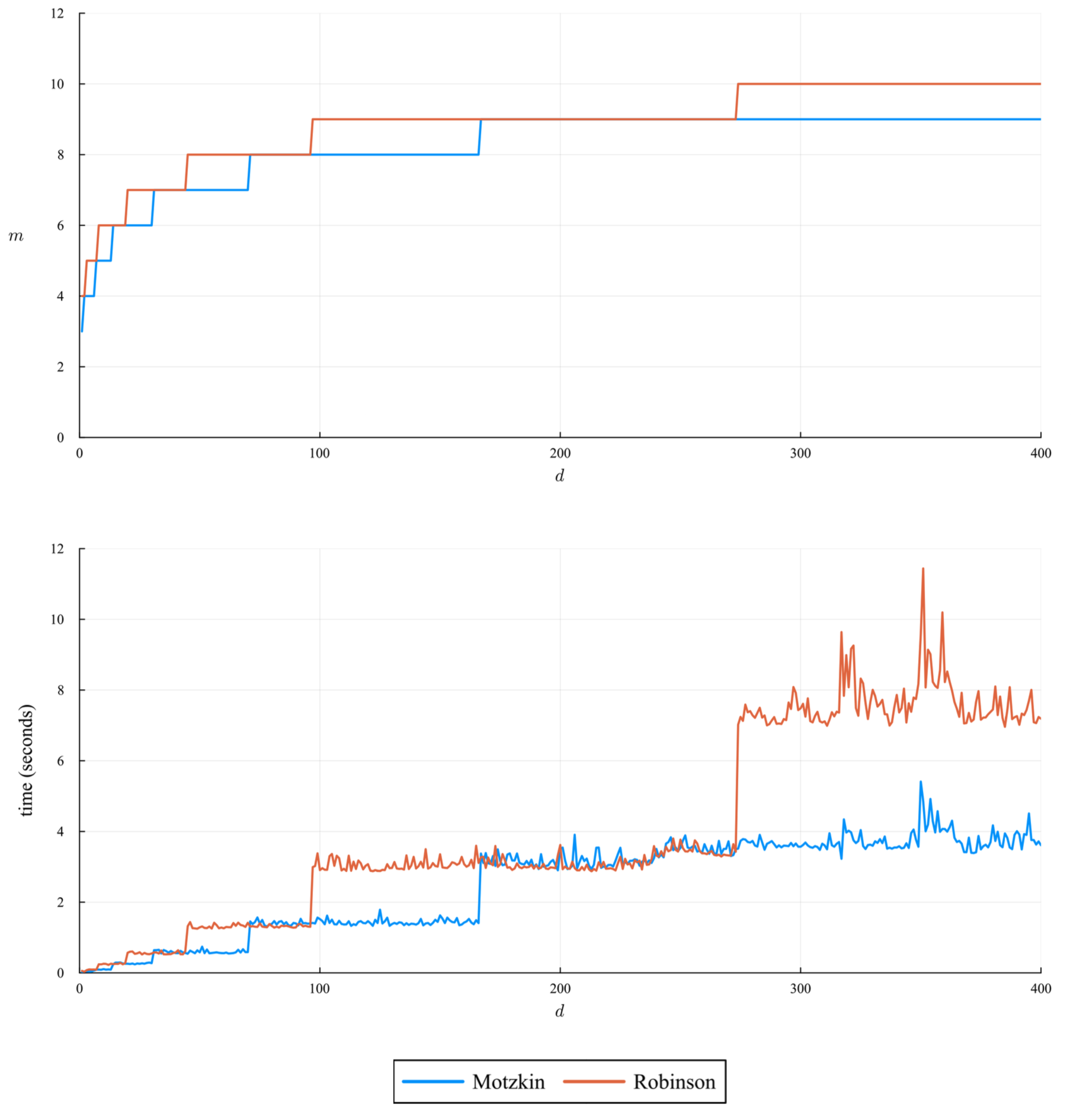
Figure 1: Performances of implementation of Algorithm 3 for modified Motkzin and Robinson polynomials

Figure 1 reports the parameter $m$ and the time (in second) used by the implementation. The parameter $m$ is the minimal degree for $f_{\epsilon}$ in (3) to become a sum of squares. The reader should note that as $d$ (horizontal axis) increases, the values of $m$ and time also increase.

7 Future work

We conclude this paper by listing several potential research problems we want to further investigate: (1) degree estimation for the certificates constructed by our method, and this may lead to interesting results for effective Putinar’s Positivstellensatz; (2) extending our method to deal with polynomials which are non-negative over $\operatorname{S}(G)$; (3) complexity analysis of Algorithm 4 and further optimization on our implementation for it; (4) identify sub cases and conditions to obtain simpler certificates.

8 Acknowlegements

The research of Weifeng Shang and Chenqi Mou was supported in part by National Natural Science Foundation of China (NSFC 12471477) and that of Jose Abel Castellanos Joo and Deepak Kapur was supported in part by U.S. National Science Foundation (CCF-1908804).

References

- [1] Gennadiy Averkov. Constructive proofs of some Positivstellensätze for compact semialgebraic subsets of . Journal of Optimization Theory and Applications, 158(2):410–418, 2013.
- [2] Lorenzo Baldi and Bernard Mourrain. On the effective Putinar’s Positivstellensatz and moment approximation. Mathematical Programming, 200(1):71–103, 2023.
- [3] Christian Berg. The multidimensional moment problem and semigroups. In Proceedings of Symposia in Applied Mathematics, volume 37, pages 110–124, 1987.
- [4] Jacek Bochnak, Michel Coste, and Marie-Françoise Roy. Real Algebraic Geometry, volume 36. Springer Science & Business Media, 2013.
- [5] David Hilbert. Ueber die Darstellung definiter Formen als Summe von Formenquadraten. Mathematische Annalen, 32(3):342–350, 1888.
- [6] Jean B Lasserre. A sum of squares approximation of nonnegative polynomials. SIAM Review, 49(4):651–669, 2007.
- [7] Monique Laurent and Lucas Slot. An effective version of Schmüdgen’s Positivstellensatz for the hypercube. Optimization Letters, 17(3):515–530, 2022.
- [8] Victor Magron and Mohab Safey El Din. RealCertify: a Maple package for certifying non-negativity. ACM Communications in Computer Algebra, 52(2):34–37, 2018.
- [9] Victor Magron and Mohab Safey El Din. On exact Polya and Putinar’s representations. In Proceedings of the 2018 ACM International Symposium on Symbolic and Algebraic Computation, pages 279–286, 2018.
- [10] Murray Marshall. Positive Polynomials and Sums of squares. Number 146. American Mathematical Society, 2008.
- [11] Jiawang Nie and Markus Schweighofer. On the complexity of Putinar’s Positivstellensatz. Journal of Complexity, 23(1):135–150, 2007.
- [12] Victoria Powers. Positive polynomials and sums of squares: Theory and practice. Real Algebraic Geometry, 1:78–149, 2011.
- [13] Victoria Powers and Bruce Reznick. Polynomials that are positive on an interval. Transactions of the American Mathematical Society, 352(10):4677–4692, 2000.
- [14] Victoria Powers and Bruce Reznick. A new bound for Pólya’s Theorem with applications to polynomials positive on polyhedra. Journal of Pure and Applied Algebra, 164(1–2):221–229, 2001.
- [15] Mihai Putinar. Positive polynomials on compact semi-algebraic sets. Indiana University Mathematics Journal, 42(3):969–984, 1993.
- [16] Konrad Schmüdgen. The K-moment problem for compact semi-algebraic sets. Mathematische Annalen, 289(1):203–206, 1991.
- [17] Markus Schweighofer. An algorithmic approach to Schmüdgen’s Positivstellensatz. Journal of Pure and Applied Algebra, 166(3):307–319, 2002.
- [18] Markus Schweighofer. On the complexity of Schmüdgen’s Positivstellensatz. Journal of Complexity, 20(4):529–543, 2004.
- [19] Markus Schweighofer. Optimization of Polynomials on Compact Semialgebraic Sets. SIAM Journal on Optimization, 15(3):805–825, 2005.
- [20] Gilbert Stengle. Complexity Estimates for the Schmüdgen Positivstellensatz. Journal of Complexity, 12(2):167–174, 1996.