A controllable theory of superconductivity due to strong repulsion in a polarized band

Abstract

Can strong repulsive interaction be shown to give rise to pairing in a controllable way? We find that for a single flavor polarized band, there is a small expansion parameter in the low density limit, once the Bloch wavefunction overlap is taken into account. A perturbative expansion is possible, even if the interaction is much stronger than the Fermi energy $\epsilon_{F}$. We illustrate our method with a two-band model that is often used to describe multi-layer rhombohedral graphene and comment on the relationship with experiments. This work opens a reliable pathway to search for topological superconductors with high-$T_{c}$ (relative to $\epsilon_{F}$) in materials with strongly interactions. We summarize the requirements and suggest some illustrative design structures.

Strong electron–electron interactions in correlated quantum systems can drive spontaneous symmetry breaking of electronic flavor degrees of freedom via Stoner-type transitions. Recent experiments have observed this phenomenon in two-dimensional flatband platforms, including twisted graphene [1, 2, 3, 4, 5], untwisted graphene multilayers[6, 7, 8, 9, 10], and moiré-patterned transition metal dichalcogenides[11, 12]. These systems exhibit interaction-driven cascades of spontaneous spin and valley polarization, often leading to a fully flavor polarized state where all electrons occupy a single spin and valley. This maximally polarized phase is found to host a rich array of exotic many-body phenomena, such as superconductivity, fractional quantum anomalous Hall states, and Wigner crystal formation [13, 14].

These experiments motivate us to study the possibility of superconducting pairing in the presence of strong repulsion, whose energy can be much larger than the Fermi energy, as dictated by the occurrence of Stoner instability to begin with. There are not many examples where pairing instability has been demonstrated starting with a purely repulsive interaction. The early work by Kohn and Luttinger [15] made use of the $2k_{F}$ singularity to show that in 3D there is attraction in some high angular momentum channel $l$ in second order perturbation which can overwhelm the first order repulsion for some large $l$. Since this is a large $l$ expansion, $T_{c}\approx\epsilon_{F}\exp(-1/g)$ is exponentially small because $g\propto 1/l^{4}$. Furthermore it does not work in 2D because the singularity exists only for $k>k_{F}.$ (For a review and extension to magnetic field polarized bands, see [16, 17].) Recently some special models on honeycomb lattices have been shown to have pairing [18, 19], but a general controllable treatment in the presence of strong repulsion seems out of reach.

To tackle this problem, a common approach is to use the random phase approximation (RPA), which keeps track of the screening of the repulsion between electrons, but ignores other high-order terms. The screened electron-electron interaction $V=\frac{V_{0}}{1+V_{0}\Pi}$ where $\Pi$ is the polarization bubble, saturates at $1/\Pi$ regardless of how strong the bare interaction $V_{0}$ is. This screened interaction therefore gives an order-1 coupling constant. Recently, several theories [20, 21, 22, 23, 24] use the RPA approach in flavor-polarized tetralayer and pentalayer graphene to explain the superconductivity observed in these systems[14]. However, this approach is not justified for fully polarized systems: there is no good reason to single out the screening processes while neglecting other processes such as vertex corrections, cross diagrams, etc. In fact, at each order of the coupling constant expansion, these types of diagrams should have comparable contributions, so what RPA accounts for is only a small part of the whole story.

In this paper, we take advantage of a special property of a fully polarized band: Fermi statistics keep electrons apart, so that a short range delta function repulsion has no effect. By slightly relaxing the delta function we show that there is a small expansion parameter in the low density limit, when the Fermi momentum is much less than a characteristic momentum scale of the repulsive interaction. By including the Bloch wavefunction, we show that a substantial superconducting $T_{c}$ can be calculated in a controlled way.

To start, we consider a charge-charge repulsion in fully flavor-polarized electrons:

$$H_{int}=\frac{1}{2}\sum_{{\boldsymbol{q}}}V_{{\boldsymbol{q}}}\rho_{{\boldsymbol{q}}}\rho_{-{\boldsymbol{q}}},\quad\rho_{{\boldsymbol{q}}}=\sum_{{\boldsymbol{k}}}\Lambda_{{\boldsymbol{k}},{\boldsymbol{k}}+{\boldsymbol{q}}}c^{\dagger}_{{\boldsymbol{k}}}c_{{\boldsymbol{k}}+{\boldsymbol{q}}}.$$ (1)

where the structure factor $\Lambda_{{\boldsymbol{k}},{\boldsymbol{k}}+{\boldsymbol{q}}}=\langle u_{{\boldsymbol{k}}}|u_{{\boldsymbol{k}}+{\boldsymbol{q}}}\rangle$, here $|u_{{\boldsymbol{k}}}\rangle$ represents the Bloch wavefunction. We start from a simplest case of electrons in tight-binding one-band model with a contact interaction, so that Bloch wavefunction and interaction are both independent of momentum: i.e. $|u_{{\boldsymbol{k}}}\rangle=1$ and $V_{{\boldsymbol{q}}}=V_{0}$. For this case, one finds the interaction effect completely vanishes through a perfect cancellation between direct and exchange processes (see Fig.1(a) that always come in a package at any order of diagrammatic expansion. This is reasonable as Pauli exclusion does not allow electrons in one flavor to interact through a contact interaction.

This motivates us to consider a small modification of this trivially solvable case in two steps.

1. We introduce some momentum-dependence by truncating the repulsion $V_{{\boldsymbol{q}}}$ at a momentum $q_{d}$ such that $k_{F}\ll q_{d}\ll G_{0}$, where $G_{0}$ is the shortest reciprocal lattice vector i.e.

   $$V_{{\boldsymbol{q}}}=V_{0}\Theta(q_{d}-|{\boldsymbol{q}}|).$$ (2)

   This can be realized by an adjacent metallic gate at a distance $d=1/q_{d}$.

2. With Eq. 2, the interaction still exactly cancels if the Bloch function $u_{{\boldsymbol{k}}}$ is independent of ${{\boldsymbol{k}}}$, as in the case of a tight-binding band with a single orbital. A non-vanishing effect comes from a weak $k$-dependence in the Bloch wave function, “weak” in the sense that the amplitude of $k$-dependent part of wavefunction is much smaller than the $k$-independent part. That will be the case for a general LDA type band when $k_{F}\ll G_{0}$. Alternatively, we need a multi-band tight binding Hamiltonian.

It is important to note that Step(1) is not really a “small” modification of the interaction in that it turns a delta function repulsion on the sub-lattice scale to one that extends over several unit cells. All higher umklapp processes needed to recover the delta function interaction has been ignored. However, this has almost no impact on the low-energy physics. This is because the scattering processes that are relevant for low-energy physics are those with all the electron’s momenta restricted within $O(k_{F})$.

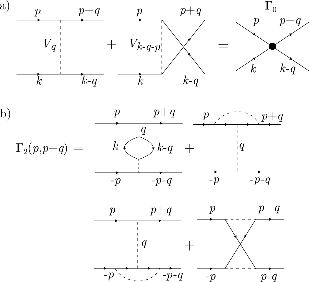
Figure 1: a) The first order diagram consists of direct repulsion and exchange. The total scattering amplitude $\Gamma_{0}$ (the filled circle) is much smaller than each single diagram due to weak momentum dependence of wavefunction and $V_{q}$ (see text around Eq.(3) and Eq.(4)). The 1st-order pairing interaction $\Gamma_{1}$ can be obtained by setting $k$ to be $-p$ in the first diagram in a). Here, $k=(\omega,{\boldsymbol{k}})$. b) The second-order pairing interaction $\Gamma_{2}$ is the sum of four diagrams (bubble, vertex correction and cross diagrams).

With Step(2), the cancellation between exchange and direct diagrams in Fig. 1a) becomes imperfect. Namely, the total scattering amplitude of two electrons at ${\boldsymbol{k}},{\boldsymbol{p}}$ to ${\boldsymbol{k}}+{\boldsymbol{q}}$ and ${\boldsymbol{p}}-{\boldsymbol{q}}$ ($|{\boldsymbol{k}}|,|{\boldsymbol{p}}|,|{\boldsymbol{q}}|\lesssim k_{0}$) through direct and exchange processes is given by

$$\Gamma_{0}({\boldsymbol{k}},{\boldsymbol{p}},{\boldsymbol{q}})=V_{0}\left[\Lambda_{{\boldsymbol{k}},{\boldsymbol{k}}+{\boldsymbol{q}}}\Lambda_{{\boldsymbol{p}},{\boldsymbol{p}}-{\boldsymbol{q}}}-\Lambda_{{\boldsymbol{k}},{\boldsymbol{p}}-{\boldsymbol{q}}}\Lambda_{{\boldsymbol{p}},{\boldsymbol{k}}+{\boldsymbol{q}}}\right]$$ (3)

This amplitude $\Gamma_{0}$ is nonvanishing and comparable to $V_{0}$ for generic ${\boldsymbol{k}}$-dependent $|u_{{\boldsymbol{k}}}\rangle$. However, for dilute electrons , this non-vanishing total scattering amplitude $\Gamma_{0}$ is controlled by a new small parameter. To see this explicitly, we use a two band model where the Fermi level lies in the band which is flat and separated by an energy gap to the other band. To estimate the amplitude $\Gamma_{0}$, we express the Bloch wavefunction in terms of its constant part and $k$-dependent part: $|u_{{\boldsymbol{k}}}\rangle=\sqrt{1-|\alpha_{{\boldsymbol{k}}}|^{2}}|v_{0}\rangle+\alpha_{{\boldsymbol{k}}}|v_{1}\rangle$, where $|v_{0}\rangle$ represents an “average” Bloch wavefunction; $|v_{1}({\boldsymbol{k}})\rangle$ is orthogonal to $|v_{0}\rangle$, representing the variation of wavefunction; $|\alpha_{k}|$ represents the magnitude of wavefunction’s variation, which is small for $k\lesssim O(k_{F})$ due to smallness of $k_{F}$. Assuming the wavefunction has an order-1 variation on some momentum scale $k_{*}$, the parameter $|\alpha_{k_{F}}|$ is small in $k_{F}/k_{*}$ ($k_{*}$ is expected to be $G_{0}$ or larger for a generic band, and is roughly $G_{0}$ for a generic Chern band. It is of order the inverse of the magnetic length $l_{B}$ for a Landau level). In other words, the new parameter $|\alpha_{k}|$ can be expressed in terms of the quantum metric $g_{ij}$ as roughly $\sim{\rm\,Tr\,}(g_{ij})k_{F}^{2}$. In the presence of a Berry curvature, $g_{ij}$ is not small and we rely on the smallness of $k_{F}$ to get a small parameter. More generally, $g_{ij}$ depends on details of the Bloch band. Plugging the expression of wavefunction $|u_{k}\rangle$ into Eq.(3) we find

$$\Gamma_{0}({\boldsymbol{k}},{\boldsymbol{p}},{\boldsymbol{q}})\sim O(|\alpha_{k_{F}}|^{2}V_{0})$$ (4)

which can be much smaller than $V_{0}$. Therefore, the effective strength of coupling in this system is described by the average of the total vertex $\Gamma_{0}$ (rather than the original vertex $V_{0}$) on the Fermi surface:

$$g_{\rm eff}=\nu_{0}\int\frac{d\theta_{p}d\theta_{p^{\prime}}}{(2\pi)^{2}}\Gamma_{0}({\boldsymbol{p}},{\boldsymbol{p}}’,0),$$ (5)

where $\theta_{p}$ is the polar angle of ${\boldsymbol{p}}$, the integrals over ${\boldsymbol{p}},{\boldsymbol{p}}^{\prime}$ are taken along Fermi surface and $\nu_{0}$ is the density of states. Even if the original coupling $g_{0}=\nu_{0}V_{0}\gg 1$, there still exists a regime of $\alpha_{k_{F}}$ such that the effective coupling constant $g_{\rm eff}$ is still sufficiently weak so that a controllable analysis through a perturbative expansion is possible.

The reader may be concerned that the bare interaction remains strong and may appear in other diagrams outside of the pairing channel considered below. Here we appear to Landau’s Fermi liquid theory which states that interaction effects, no matter how strong, that are far away from the Fermi surface only give rise to renormalized parameters such as effective mass and coupling strength for the low energy quasi-particles. Hence our treatment only deals with pairing of quasi-particles in the Landau sense and the bare interactions are treated as renormalized parameters which remains strong.

Model: Below we demonstrate this idea through a concrete model. We consider an $N$-Dirac model with following noninteracting Hamiltonian

$$H_{0}({\boldsymbol{p}})=\left(\begin{matrix}\frac{u}{2}&\frac{u\left(p_{x}-ip_{y}\right)^{N}}{2k_{0}^{N}}\\ \frac{u\left(p_{x}+ip_{y}\right)^{N}}{2k_{0}^{N}}&-\frac{u}{2}\end{matrix}\right)$$ (6)

Here $N$ can take integer values $N=1,2,3,4...$ while $u$ sets the gap between two bands and flattened them. The momentum $k_{0}$ sets the radius of the flattened band bottom(top). For $|{\boldsymbol{p}}|$ exceeding this scale, the band dispersion becomes steep. Without losing generality, we focus on the electron-doped case ($n>0$) throughout our analysis. The Bloch wavefunction in the electron band is given by $|u_{{\boldsymbol{k}}}\rangle=(\sqrt{1-|\alpha_{{\boldsymbol{k}}}|^{2}},|\alpha_{{\boldsymbol{k}}}|e^{iN\theta_{{\boldsymbol{k}}}})$ with $\theta_{{\boldsymbol{k}}}$ representing the angle of ${\boldsymbol{k}}$, $|\alpha_{{\boldsymbol{k}}}|\sim\frac{1}{2}(|{\boldsymbol{k}}|/k_{0})^{N}$ for $|{\boldsymbol{k}}|\ll k_{0}$. We note in passing that this model is a widely used as a toy model for real systems such as rhombohedral graphene with N layer (see e.g.[21]). Remarkably, SC phases are indeed seen in flavor-polarized phases in some of these systems. [14] We will come back to comment on this connection in Appendix A.

Pairing interaction: Using this model, we now proceed to study pairing in flavor-polarized electrons using the controllable perturbation theory outlined above. In this framework, the pair-scattering processes first and second order in $V_{0}$ can be expressed as diagrams in Fig.1. The first-order pair interaction is given by

$$\Gamma_{1}({\boldsymbol{p}},{\boldsymbol{p}}^{\prime})=V_{0}\langle u_{{\boldsymbol{p}}}|u_{{\boldsymbol{p}}^{\prime}}\rangle\langle u_{-{\boldsymbol{p}}}|u_{-{\boldsymbol{p}}^{\prime}}\rangle$$ (7)

While $\Gamma_{1}$ is comparable to $V_{0}$, the effective pairing interaction is implicitly small in $\alpha_{k_{F}}$. This is because, due to Fermion statistics, in $\Gamma_{1}$ only its antisymmetric part is useful for pairing. The antisymmetric part is given by, $\frac{1}{2}\left(\Gamma_{1}(\omega-\omega^{\prime};{\boldsymbol{p}},{\boldsymbol{p}}^{\prime})-\Gamma_{1}(\omega+\omega^{\prime};{\boldsymbol{p}},-{\boldsymbol{p}}^{\prime})\right)$, which is equivalent to the two diagrams in Fig.1a), therefore has the same cancellation as $\Gamma_{0}$. The second-order pairing interaction is implicitly $\propto\Gamma_{0}^{2}$, and is thus higher-order in terms of the small parameter $\alpha_{k_{F}}$. This is expected but may not be easy to see from Fig.1b). To make this more explicit, we note that the sum of four diagrams in Fig.1b) is equivalent to one bubble diagram with its two vertices replaced by two $\Gamma_{0}$’s.

Interestingly, for even-$N$ Dirac model ($N=2,4,6...$), the wavefunction has the following symmetry: $|u_{{\boldsymbol{p}}}\rangle=|u_{-{\boldsymbol{p}}}\rangle$. Therefore, the antisymmetrized pairing interaction $\frac{1}{2}\left(\Gamma_{1}({\boldsymbol{p}},{\boldsymbol{p}}^{\prime})-\Gamma_{1}({\boldsymbol{p}},-{\boldsymbol{p}}^{\prime})\right)$ always vanishes. As a result, the pairing interaction in even-$N$ Dirac model is dominated by second-order processes in Fig.1 b). In comparison, in odd-$N$ Dirac model ($N=1,3,5...$) the two first-order diagrams do not cancel each other, so $\Gamma_{1}$ is the leading order contribution.

Pairing channels and $T_{c}$: Now, we proceed to analyze the pairing problem. We will first study the pairing channel and the behavior of $T_{c}$ in Dirac model with a general integer value of $N$, and then obtain the $T_{c}$ in even-$N$ and odd-$N$ Dirac models separately. To start, we write down the linearized pairing gap equation:

$$\Delta(\omega,{\boldsymbol{p}})=T_{c}\sum_{\omega^{\prime},{\boldsymbol{p}}^{\prime}}\frac{\Gamma(\omega,\omega^{\prime};{\boldsymbol{p}},{\boldsymbol{p}}^{\prime})\Delta(\omega^{\prime},{\boldsymbol{p}}^{\prime})}{\omega^{\prime 2}+\epsilon_{{\boldsymbol{p}}^{\prime}}^{2}}$$ (8)

where $\Gamma$ is the two particle irreducible pairing interaction, whose first-order contribution is given in Eq.(7) and second-order contribution is $\Gamma_{2}$ expressed diagrammatically in Fig.1b). To proceed, we neglect the radial momentum-dependence of $\Delta$ and integrating along the direction perpendicular to Fermi surface $p_{\perp}$. Reparameterizing momenta ${\boldsymbol{p}},{\boldsymbol{p}}^{\prime}$ using the angle $\theta,\theta^{\prime}$ on Fermi surface yields:

$$\Delta(\omega;\theta)=\pi\nu_{0}T_{c}\sum_{\omega^{\prime}}\int\frac{d\theta^{\prime}}{2\pi}\frac{\Gamma(\omega,\omega^{\prime};\theta,\theta^{\prime})\Delta(\omega^{\prime};\theta^{\prime})}{|\omega^{\prime}|}$$ (9)

In our setting, $\Gamma(\theta,\theta^{\prime})$ is a function of $\theta-\theta^{\prime}$ as dictated by the U(1) symmetry of Dirac models (spatial rotation + a relative phase shift between AB sublattice). This allows labeling pairing channels with angular momenta $l$ which is a good quantum number:

$$\Delta^{(l)}(\omega)=\pi\nu_{0}T_{c}\sum_{\omega^{\prime}}\frac{\Gamma^{(l)}(\omega,\omega^{\prime})\Delta^{(l)}(\omega^{\prime})}{|\omega^{\prime}|},\quad l\in\mathcal{Z}.$$ (10)

Here we have defined the partial wave components: $\Delta^{(l)}(\omega)=\int\frac{d\theta}{2\pi}\Delta(\omega;\theta)e^{il\theta}$ and $\Gamma^{(l)}(\omega-\omega^{\prime})=\int\frac{d(\theta-\theta^{\prime})}{2\pi}\Gamma(\omega-\omega^{\prime};\theta-\theta^{\prime})e^{il(\theta-\theta^{\prime})}$. In Eq.(10), angular momentum $l$ is allowed to take either even or odd values. However, due to fermion statistic, the odd-parity pairing channels (i.e. channels with odd-valued $l$) have to be even in frequency, whereas the even-parity pairing channels have to be odd in frequency: $\Delta^{(l)}(\omega)=-\Delta^{(l)}(-\omega),l\in{\rm even}$.[25, 26] Below we work out the $T_{c}$ of even-frequency and odd-frequency channels separately:

For even-frequency odd-$l$ pairing, the solution of gap equation is similar to BCS problem, except that the bandwidth of pairing interaction, which is Debye frequency in BCS problem, is replaced with $\epsilon_{F}$, as the pairing interaction in our problem arises from 2nd-order diagram in Fig.1 which inherit the frequency dependence of the polarization bubble. Therefore, just like in BCS problem, the gap equation here can also be solved by replacing $\Gamma^{(l)}(\nu)$, which is an even function of frequency $\nu$ for $l\in{\rm odd}$, with $\Gamma^{(l)}(\nu)=\Gamma^{(l)}(0)\Theta(\epsilon_{F}-|\nu|)$. We define the dimensionless coupling constant $g^{(l)}=\nu_{0}\Gamma^{(l)}(0)$ for both even and odd $l$. They are plotted in the insets in Fig. 2 (a,b) for N=2 and 4. We find that $g^{(l)}$ are mostly positive, indicating attraction, and have a strong peak near $l=2N$. Its origin can be traced back to the fact that $\Gamma_{0}$ given by Eq. 3 has two factors of $\Lambda$. When all the momenta in the $\Lambda$’s are on the Fermi surface, there is an $e^{iN\theta}$ contribution to $\Gamma_{0}$ where $\theta$ is the angle between ${\boldsymbol{k}}$ and ${\boldsymbol{k}}^{\prime}$. To second order in $\Gamma_{0}$ we obtain a factor $e^{i2N\theta}$. This feature is specific to the $N$-Dirac model. The large peak for $g^{(l)}$ for even $l=2N$ does not contribute to conventional even frequency BCS pairing, which can make use of only of the largest odd $l$. Nevertheless, the strong $l=2N$ peak leads us to consider odd frequency pairing below.

Solving the gap equation for odd $l$ yields the standard BCS superconducting $T_{c}$

$$T_{c}^{(l)}\sim 1.13\epsilon_{F}\exp\left(-\frac{1}{g^{(l)}}\right),\quad l\in{\rm odd}$$ (11)

We find the leading pairing channel is $l=3$ for $N=2$ Dirac model, and is $l=7$ for $N=4$ Dirac model. This is reasonable because the pairing interaction is maximized for odd values of $l$ that are closest to $2N$. (see insets of Fig.2). These are topological superconductors where the gap function goes as $e^{il\theta}$.

The odd-frequency channels do not have a BCS logarithm in its susceptibility [26, 25], and instability is expected to occur above a finite threshold of coupling strength. To solve this threshold analytically, we model the frequency dependence of $\Gamma(\omega)$ using the following separable form:

$$\Gamma^{(l)}(\omega-\omega^{\prime}) =\Gamma_{1}^{(l)}+\Omega(\omega-\omega^{\prime})\Gamma^{(l)}_{2}(0),\quad l\in{\rm even}$$ (12)

$$\Omega(\omega) =\frac{1}{\mathcal{N}}\int\frac{\tau e^{i\frac{\omega}{\epsilon_{F}}\tau}d\tau}{\rm{erfi}(\frac{\tau}{\sqrt{2}})},$$

where ${\rm erfi}(x)=\frac{2}{\sqrt{\pi}}\int^{x}_{0}\exp(z^{2})dz$, $\mathcal{N}=4.6362$ is the normalization coefficient that makes $\Omega(0)=1$. Here, we isolated first-order contribution $\Gamma_{1}$ which is frequency-independent and therefore do not contribute to odd-frequency pairing. We chose this separable form as a model for $\Gamma_{2}^{(l)}(\omega)$ because it mimics the realistic bandwidth of 2nd-order interaction ($\sim\epsilon_{F}$) and meanwhile keeps the gap equation analytically solvable. Using Eq.(12), we find the following form of gap function is the odd-in-$\omega$ even-$l$ solution of $T=0$ linearized gap equation [See Appendix C] :

$$\Delta^{(l)}(\omega)=\omega\exp(-\omega^{2}/2\epsilon_{F}^{2}),\quad l\in{\rm even}$$ (13)

Plugging Eq.(13) into the $T=0$ gap equation yields:

$$1=\frac{\pi}{\mathcal{N}}g_{2}^{(l)},\quad l\in{\rm even}$$ (14)

where $g_{2}^{(l)}=\nu_{0}\Gamma_{2}^{(l)}(0)$. This equation gives the onset condition for odd-frequency SC: $g_{2}^{(l)}=\mathcal{N}/\pi=1.48$. Once coupling $g_{2}^{(l)}$ exceeds this threshold, we expect that $T_{c}$ should quickly rise to $O(\epsilon_{F})$ and saturates. We analyzed more carefully the behavior of $T_{c}$ within this model (Eq.(12)), but we leave the details to Appendix B, as the results are approximate and depend on the specific form of $\Gamma(\omega)$ we chose. We note that odd frequency pairing is gapless because $\Delta(\omega=0)=0$, and is not expected to be topological, unlike the even frequency pairing.

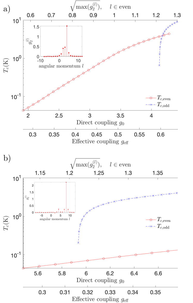
Figure 2: Dependence of $T_{c}$ on interaction strength for a) $N=2$ Dirac model and b) $N=4$ Dirac model. Red and blue curves represent $T_{c}$ in the leading even-frequency and odd-frequency channels respectively. In the bottom x-axis, we map out the value of the bare and effective couplings $g_{0},g_{\rm eff}$ defined in Eq.5 . The top x-axis shows the coupling strength in the leading odd-frequency pairing channel $\max(g^{(l)}_{2})$ with $l$ restricted to be an even integer[27]. Results in both panels are calculated at $n=5\times 10^{-3}{\rm nm}^{-2}$, $u=80{\rm meV}$, $k_{0}=0.34{\rm nm}^{-1}$. The Fermi energy in two cases are $\epsilon_{F}=5.51{\rm meV}$ for a) and $\epsilon_{F}=1.75{\rm meV}$ for b). In the regimes shown, despite the naive coupling $g_{0}\gg 1$, the effective coupling $g_{\rm eff}$ is below 1, so the perturbation theory is controllable. The insets show the angular momentum components of the pairing interaction. It is maximized at $l=4$ in $N=2$ Dirac model, and at $l=8$ in the $N=4$ one.

The analysis so far is applicable to Dirac models with arbitrary integer value of $N$. However, the strength of pairing interaction $\Gamma^{(l)}$ can be quite different for even and odd values of $N$ because, as discussed around Eq.(7), a crucial difference between even-$N$ and odd-$N$ Dirac models is whether the first-order processes contribute to pairing interaction. So below we analyze two types of models separately.

For even-$N$ Dirac model, in the controllable regime $g_{\rm eff}\ll 1$, the pairing interaction $\Gamma^{(l)}$ is just given by the 2nd order diagrams in Fig.1b) due to the cancellation of 1st order process. We numerically calculate this pairing interaction, and obtain the $T_{c}$ of even-frequency and odd-frequency channels as a function of interaction strength, as shown in Fig.4. We find the $T_{c}$ of even-frequency channel is a small fraction of $\epsilon_{F}$ since $\Gamma^{(l)}$ is small for odd-valued $l$ , but can nevertheless be a substantial fraction in the regime where the theory is controlled. For increasing repulsive strength, this is eventually taken over by odd frequency pairing. However, this is in the strong coupling regime, so our results can only be taken as a rough indication.

For the odd-$N$ Dirac model, as discussed after Eq.(7), the pairing interaction for even-frequency channel is dominated by the first-order process in the controllable regime. The first-order process is repulsive and does not support pairing. However, the first-order pairing interaction has no frequency dependence and does not contribute to odd-frequency pairing. Therefore, odd-frequency pairing may occur in the same way as in the even-$N$ Dirac model if the coupling is strong enough.

To summarize, the even-$N$ Dirac model may have both even and odd-frequency pairings, whereas for the odd-$N$ Dirac model, odd-frequency pairing is the only possibility. We note parenthetically that, in both cases, the odd-frequency pairing is not guaranteed to occur, as it is achieved in our model at a coupling close to $1$ where the controllability of perturbative analysis becomes marginal. Furthermore, the exact onset of odd-frequency pairing is nonuniversal and depends on the frequency dependence of $\Gamma$. Therefore, we do not predict definitively on whether odd-frequency channel can occur. However, our prediction of even-frequency pairing in even-$N$ Dirac model is solid, as it is safely in the controllable regime. We end by noting that this conclusion depends on the assumption of a bare interaction $V_{q}$ of the form given in Eq. 2. If there is substantial $q$ dependence on the scale of $k_{F}$, the first order process does not cancel and can be expected to be repulsive, which will tend to suppress pairing.

Finally, we emphasize that the mechanism we propose to create a topological superconductor is more general than the toy model discussed above. The requirements are: (1) a fully polarized band with low carrier density; (2) proximity to a screening metallic plane. (3) inversion symmetry so that $|u_{{\boldsymbol{p}}}\rangle=|u_{-{\boldsymbol{p}}}\rangle$ , which ensures that the first order repulsive term is cancelled. Unlike the toy model, inversion symmetry is commonplace if the band is located at the zone center. These requirements can be designed and realized in various settings. For example, in addition to gating, we can envision layer by layer growth of ferromagnetic low carrier density layers separated by conventional metals that act as screening planes, with a distance $d$ that can be nanometer or less, especially for van der Waals stacking. The ferromagnetism can be due to Stoner instability or exchange coupling to ferromagnetically aligned local moments. Low density carrier can be introduced by charge transfer from the metal. The leading interaction will likely have an attractive channel because second order perturbation theory is attractive. In this way one can search for topological superconductors with a relatively high $T_{c}.$

We thank Jason Alicea, Senthil Todadri, Zhihuan Dong, Leonid Levitov, Liang Fu, Tonghang Han and Jixiang Yang for insightful discussion. Z. D. is supported by the Gordon and Betty Moore Foundation’s EPiQS Initiative, Grant GBMF8682. P.A.L. acknowledges support from DOE (USA) office of Basic Sciences Grant No. DE-FG02-03ER46076.

Appendix A Application to rhombohedral graphene

In this appendix, we discuss the connection between this ideal solvable model and realistic systems. Here, we focus on graphene tetralayer and pentalayer, where SC is found on top of flavor-polarized parent phase, suggesting some possible connection.

The $N=4$ Dirac model we used coincides with a toy model for tetralayer graphene. In fact, the band parameter we chose in Fig.2 b) is very close to the one used in Ref.[21] that is obtained by fitting realistic band dispersion with an $N=4$ Dirac model[28].

However, there is a question whether the realistic interaction is sufficiently short-range to obey Eq. 2, which potentially affecting the controllability. To be more specific, the realistic interaction is usually modeled as a gate-screened Coulomb interaction

$$V_{q}=e^{2}\tanh(qd)/2\epsilon_{0}\epsilon_{r}q,$$ (15)

where the screening length $d$ is the gate-to-sample distance, $d\gtrsim 20{\rm nm}$ in realistic settings. It is nearly $q$-independent only for $q<1/d$. However, a naive estimate of $k_{F}$ using the measured carrier density $n\sim 0.4\times 10^{-2}{\rm nm}^{-2}$ gives a $k_{F}\sim 0.2{\rm nm}^{-1}$ which is a few times greater than $1/d$. This suggests the interaction $V_{q}$ might not be simply viewed as $q$-independent in realistic setting. Therefore, taken at face value, there seems to be no approximate cancellation, and thus no justification for controllability.

However, when there is a tiny pocket at the K point with a $k_{F,{\rm small}}\ll 1/d$, our controllable perturbation theory becomes applicable again, as all scatterings within this tiny pocket only uses the momentum-independent part of $V_{q}$.

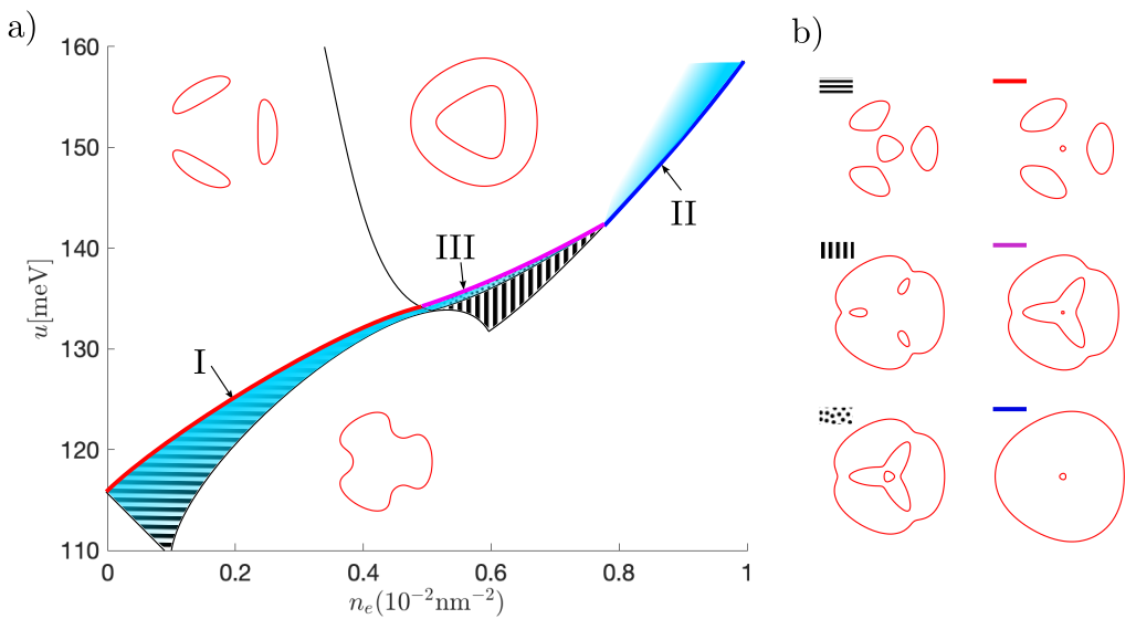
Figure 3: The prediction of SC phase position in tetralayer graphene. Insets of a) and panel b) show the fermiology of each phases obtained from the realistic eight-band model[29]. The phase boundaries I,II and III, which are highlighted in red, purple and blue respectively, are where a tiny pocket (either electron-type or hole-type pocket) emerges at the K point. In the cyan shaded regions, we expect the perturbation theory to become controllable, thus reliably predicting a superconductivity. Here the dotted phase below phase transition III is narrow, so SC there is expected to be very fragile. In comparison, the SC phases near phase boundary I and II are more stable and are likely to be visible in experiment.

Using realistic band structure, we map out the noninteracting fermiology on a phase diagram, find three situations where such tiny pocket can occur: (I) At the Lifshitz transition from three-e-pocket phase to 3+1 e-pocket phase; (II) At the Lifshitz transition from one-e-pocket phase to annular Fermi sea (i.e. one-e-pocket-one-hole-pocket phase) (III) At the Lifshitz transition where one extra e-pocket in the presence of an annular Fermi sea. (i.e. from one-e-pocket-one-hole-pocket phase to two-e-pocket-one-hole-pocket phase ). These three transitions are highlighted in phase diagram Fig.3. We expect our controllable perturbation theory to be applicable near one side of each of these lines, which is shaded cyan in Fig.3. This pattern indeed looks similar to the measured phase diagram[14] where SC1 and SC2 phases indeed occurs along a diagonal line.

There is another SC phase (called SC3 in Ref.[14]) seen near the Wigner crystal phase that occupies the lower left corner in Fig.3. We conjecture that this SC might occur in a similar way: doping a Wigner crystal gives rise to dilute itinerant carriers that form tiny pocket. It would lend further support to our scenario if there is any evidence of dilute carriers in the regime between SC3 and Wigner crystal phase.

The appearance of superconductivity is very similar in pentalayer and tetralayer graphene [14] which seems to contradict our theory. Here we note that the toy model we employ is not expected to be accurate as the layer number becomes large. In a more realistic band calculation, the electrons are known to be localized near the top two layers and not in the top and bottom layers as given in the $N$-Dirac model [30, 31, 32]. In that case, four and five layers may have similar behavior. We plan to investigate this difference with a more realistic model in the future. Meanwhile, the fact the superconductivity has not yet been seen in triple-layer graphene could be understood through the absence of even-frequency pairing in $N=3$ Dirac model in our theory.

Appendix B Detailed analysis of odd-frequency pairing channels

In main text, we have shown that odd-frequency pairing $g_{2}^{(l)}\sim O(1)$ and can reach a $T_{c}$ that is comparable to $\epsilon_{F}$. Here, we study the dependence of $T_{c}$ in odd-frequency channels on $g^{(l)}_{2}$. For that, we restore the Matsubara summation in linearized gap equation and solve it numerically. When solving it, for simplicity, we first ignore the temperature dependence of pairing interaction $\Gamma$, which we will come back to comment on shortly. The numerical result is shown in Fig.4. Here we see that SC indeed sets in when coupling strength $g^{(l)}_{2}$ exceeds a value of $0.738$ and grows with $g^{(l)}_{2}$ as expected.

However, $T_{c}$ behaves abnormally when it becomes $\sim\epsilon_{F}$: it abruptly diverges upon $g^{(l)}_{2}$ reaches a threshold of $1$. This behavior can be understood as follows. In the regime of $T_{c}\sim\epsilon_{F}$, the linearized gap equation becomes solvable again because $\Omega(\omega)$ takes nonzero values only at $\omega=0$, and therefore $W(\omega)$ is nonzero only at the two smallest nonzero Matsubara frequencies $\omega=\pm 2\pi T_{c}$. In this case, the linearized gap equation becomes

$$\Delta^{(l)}(\pm 2\pi T_{c})=T_{c}\frac{\pi\Omega(0)2g^{(l)}_{2}}{2\pi T_{c}}\Delta^{(l)}(\pm 2\pi T_{c})$$ (16)

which yields a solution of $g^{(l)}_{2}=1$, independent of $T_{c}$. It means when $g^{(l)}_{2}$ exceeds this threshold, SC can occur at any temperature, which is exactly the behavior seen in Fig.4.

However, we know that this behavior is unphysical ,as a temperature comparable to $\epsilon_{F}$ would suppress the susceptibility, thus suppress the pairing interaction. This T-dependence of pairing interaction is not accounted for in our model. Therefore, we conclude that $T_{c}$ will saturate at $O(\epsilon_{F})$.

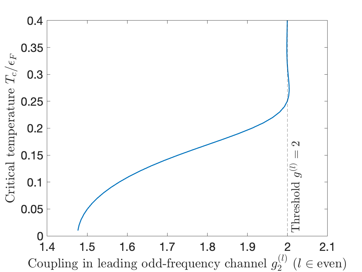
Figure 4: $T_{c}$ in odd-frequency channel as a function of coupling constant $g^{(l)}_{2}$. The behavior at $T_{c}\ll\epsilon_{F}$ agrees with analysis. The $T_{c}$ diverges at around $g^{(l)}_{2}=1$, but this is an artifact that arises due to neglecting $T$-dependence of pairing interaction in our analysis. We expect the $T_{c}$ to saturate somewhere $T\sim\epsilon_{F}$ when $T$-dependence of pairing interaction is accounted for(see text).

Appendix C Check the solution of linearized gap equation

Here we explicitly check that Eq.(13) is indeed the solution of Eq.(10). Plugging Eq.(13) back in, focusing solely on the frequency dependent parts on both left and right hand side, and Fourier transforming from frequency domain to time domain, we find the Fourier transform of left-hand side in Eq.(10) is

$$\mathcal{F}\left[{\rm LHS}\right] =\int\frac{d\omega}{2\pi}\omega\exp(-\omega^{2}/2\epsilon_{F}^{2})e^{-i\omega\tau}$$ (17)

$$=-i(2\pi)^{-1/2}\epsilon_{F}^{3}\tau e^{-\tau^{2}\epsilon_{F}^{2}/2},$$ (18)

whereas the Fourier transform of the right-hand side of Eq.(10) is

$$\mathcal{F}\left[\rm{RHS}\right] =\pi g^{(l)}_{2}\mathcal{F}\left[\Omega\right]\cdot\mathcal{F}\left[\frac{\Delta^{(l)}(\omega)}{|\omega|}\right]$$

$$=\pi g^{(l)}_{2}\left[\frac{1}{\mathcal{N}}\frac{\epsilon_{F}^{2}\tau}{\rm{erfi}(\frac{\epsilon_{F}\tau}{\sqrt{2}})}\right]\left[-i(2\pi)^{-1/2}\epsilon_{F}\exp(-\epsilon_{F}^{2}\tau^{2}/2){\rm erfi}\left(\frac{\epsilon_{F}\tau}{\sqrt{2}}\right)\right]$$

$$=-i(2\pi)^{-1/2}\frac{1}{\mathcal{N}}\pi g^{(l)}_{2}\epsilon_{F}^{3}\tau\exp(-\epsilon_{F}^{2}\tau^{2}/2)$$ (19)

Therefore, left-hand side and right -hand side indeed match when $1=\frac{\pi}{\mathcal{N}}g^{(l)}_{2}$.

References

- Cao et al. [2018a] Y. Cao, V. Fatemi, A. Demir, S. Fang, S. L. Tomarken, J. Y. Luo, J. D. Sanchez-Yamagishi, K. Watanabe, T. Taniguchi, E. Kaxiras, and et al., Correlated insulator behaviour at half-filling in magic-angle graphene superlattices, Nature 556, 80–84 (2018a).
- Cao et al. [2018b] Y. Cao, V. Fatemi, S. Fang, K. Watanabe, T. Taniguchi, E. Kaxiras, and P. Jarillo-Herrero, Unconventional superconductivity in magic-angle graphene superlattices, Nature 556, 43–50 (2018b).
- Jiang et al. [2019] Y. Jiang, X. Lai, K. Watanabe, T. Taniguchi, K. Haule, J. Mao, and E. Y. Andrei, Charge order and broken rotational symmetry in magic-angle twisted bilayer graphene, Nature 573, 91–95 (2019).
- Xie et al. [2019] Y. Xie, B. Lian, B. Jäck, X. Liu, C.-L. Chiu, K. Watanabe, T. Taniguchi, B. A. Bernevig, and A. Yazdani, Spectroscopic signatures of many-body correlations in magic-angle twisted bilayer graphene, Nature 572, 101–105 (2019).
- Zondiner et al. [2020] U. Zondiner, A. Rozen, D. Rodan-Legrain, Y. Cao, R. Queiroz, T. Taniguchi, K. Watanabe, Y. Oreg, F. von Oppen, A. Stern, et al., Cascade of phase transitions and dirac revivals in magic-angle graphene, Nature 582, 203 (2020).
- Zhou et al. [2021a] H. Zhou, T. Xie, A. Ghazaryan, T. Holder, J. R. Ehrets, E. M. Spanton, T. Taniguchi, K. Watanabe, E. Berg, M. Serbyn, and A. F. Young, Half- and quarter-metals in rhombohedral trilayer graphene, Nature 598, 429–433 (2021a).
- Zhou et al. [2021b] H. Zhou, T. Xie, T. Taniguchi, K. Watanabe, and A. F. Young, Superconductivity in rhombohedral trilayer graphene, Nature 598, 434–438 (2021b).
- Zhou et al. [2022] H. Zhou, L. Holleis, Y. Saito, L. Cohen, W. Huynh, C. L. Patterson, F. Yang, T. Taniguchi, K. Watanabe, and A. F. Young, Isospin magnetism and spin-polarized superconductivity in bernal bilayer graphene, Science 375, 774 (2022), https://www.science.org/doi/pdf/10.1126/science.abm8386 .
- Zhang et al. [2023] Y. Zhang, R. Polski, A. Thomson, É. Lantagne-Hurtubise, C. Lewandowski, H. Zhou, K. Watanabe, T. Taniguchi, J. Alicea, and S. Nadj-Perge, Enhanced superconductivity in spin–orbit proximitized bilayer graphene, Nature 613, 268–273 (2023).
- Seiler et al. [2022] A. M. Seiler, F. R. Geisenhof, F. Winterer, K. Watanabe, T. Taniguchi, T. Xu, F. Zhang, and R. T. Weitz, Quantum cascade of correlated phases in trigonally warped bilayer graphene, Nature 608, 298–302 (2022).
- Wang et al. [2020] L. Wang, E.-M. Shih, A. Ghiotto, L. Xian, D. A. Rhodes, C. Tan, M. Claassen, D. M. Kennes, Y. Bai, B. Kim, K. Watanabe, T. Taniguchi, X. Zhu, J. Hone, A. Rubio, A. N. Pasupathy, and C. R. Dean, Correlated electronic phases in twisted bilayer transition metal dichalcogenides, Nature Materials 19, 861–866 (2020).
- Regan et al. [2020] E. C. Regan, D. Wang, C. Jin, M. I. Bakti Utama, B. Gao, X. Wei, S. Zhao, W. Zhao, Z. Zhang, K. Yumigeta, M. Blei, J. D. Carlström, K. Watanabe, T. Taniguchi, S. Tongay, M. Crommie, A. Zettl, and F. Wang, Mott and generalized wigner crystal states in wse2/ws2 moiré superlattices, Nature 579, 359–363 (2020).
- Lu et al. [2024] Z. Lu, T. Han, Y. Yao, A. P. Reddy, J. Yang, J. Seo, K. Watanabe, T. Taniguchi, L. Fu, and L. Ju, Fractional quantum anomalous hall effect in multilayer graphene, Nature 626, 759 (2024).
- Han et al. [2025] T. Han, Z. Lu, Z. Hadjri, L. Shi, Z. Wu, W. Xu, Y. Yao, A. A. Cotten, O. S. Sedeh, H. Weldeyesus, J. Yang, J. Seo, S. Ye, M. Zhou, H. Liu, G. Shi, Z. Hua, K. Watanabe, T. Taniguchi, P. Xiong, D. M. Zumbühl, L. Fu, and L. Ju, Signatures of chiral superconductivity in rhombohedral graphene (2025), arXiv:2408.15233 [cond-mat.mes-hall] .
- Kohn and Luttinger [1965] W. Kohn and J. M. Luttinger, New mechanism for superconductivity, Phys. Rev. Lett. 15, 524 (1965).
- Kagan et al. [2014] M. Y. Kagan, V. V. Val’kov, V. A. Mitskan, and M. M. Korovushkin, The kohn-luttinger effect and anomalous pairing in new superconducting systems and graphene, Journal of Experimental and Theoretical Physics 118, 995–1011 (2014).
- Kagan [2016] M. Y. Kagan, Unconventional superconductivity in low density electron systems and conventional superconductivity in hydrogen metallic alloys, JETP Letters 103, 728–738 (2016).
- Slagle and Fu [2020] K. Slagle and L. Fu, Charge transfer excitations, pair density waves, and superconductivity in moiré materials, Physical Review B 102, 10.1103/physrevb.102.235423 (2020).
- Crépel and Fu [2021] V. Crépel and L. Fu, New mechanism and exact theory of superconductivity from strong repulsive interaction, Science Advances 7, 10.1126/sciadv.abh2233 (2021).
- Chou et al. [2024] Y.-Z. Chou, J. Zhu, and S. D. Sarma, Intravalley spin-polarized superconductivity in rhombohedral tetralayer graphene (2024), arXiv:2409.06701 [cond-mat.supr-con] .
- Geier et al. [2024] M. Geier, M. Davydova, and L. Fu, Chiral and topological superconductivity in isospin polarized multilayer graphene (2024), arXiv:2409.13829 [cond-mat.supr-con] .
- Yang and Zhang [2024] H. Yang and Y.-H. Zhang, Topological incommensurate fulde-ferrell-larkin-ovchinnikov superconductor and bogoliubov fermi surface in rhombohedral tetra-layer graphene (2024), arXiv:2411.02503 [cond-mat.supr-con] .
- Qin and Wu [2024] Q. Qin and C. Wu, Chiral finite-momentum superconductivity in the tetralayer graphene (2024), arXiv:2412.07145 [cond-mat.supr-con] .
- Jahin and Lin [2024] A. Jahin and S.-Z. Lin, Enhanced kohn-luttinger topological superconductivity in bands with nontrivial geometry (2024), arXiv:2411.09664 [cond-mat.supr-con] .
- Berezinskii [1974] V. Berezinskii, New model of the anisotropic phase of superfluid he 3, JETP Lett. 20 (1974).
- Linder and Balatsky [2019] J. Linder and A. V. Balatsky, Odd-frequency superconductivity, Rev. Mod. Phys. 91, 045005 (2019).
- myf [a] In this figure, we used as the variable in x-axis because this quantity scales linearly with .
- myf [b] In [M. Geier, M. Davydova and L. Fu,2024] the parameter was obtained by fiiting realistic band structure with a quadratic Dirac model plus a parabolic term. The pameter we chose here corresponds to the point where prefactor of parabolic term vanishes.
- Ghazaryan et al. [2023] A. Ghazaryan, T. Holder, E. Berg, and M. Serbyn, Multilayer graphenes as a platform for interaction-driven physics and topological superconductivity, Phys. Rev. B 107, 104502 (2023).
- Dong et al. [2024a] Z. Dong, A. S. Patri, and T. Senthil, Stability of anomalous hall crystals in multilayer rhombohedral graphene, Physical Review B 110, 10.1103/physrevb.110.205130 (2024a).
- Dong et al. [2024b] Z. Dong, A. S. Patri, and T. Senthil, Theory of quantum anomalous hall phases in pentalayer rhombohedral graphene moiré structures, Physical Review Letters 133, 10.1103/physrevlett.133.206502 (2024b).
- Dong et al. [2024c] J. Dong, T. Wang, T. Wang, T. Soejima, M. P. Zaletel, A. Vishwanath, and D. E. Parker, Anomalous hall crystals in rhombohedral multilayer graphene. i. interaction-driven chern bands and fractional quantum hall states at zero magnetic field, Physical Review Letters 133, 10.1103/physrevlett.133.206503 (2024c).