Understanding Flatness in Generative Models: Its Role and Benefits

Abstract

Flat minima, known to enhance generalization and robustness in supervised learning, remain largely unexplored in generative models. In this work, we systematically investigate the role of loss surface flatness in generative models, both theoretically and empirically, with a particular focus on diffusion models. We establish a theoretical claim that flatter minima improve robustness against perturbations in target prior distributions, leading to benefits such as reduced exposure bias—where errors in noise estimation accumulate over iterations—and significantly improved resilience to model quantization, preserving generative performance even under strong quantization constraints. We further observe that Sharpness-Aware Minimization (SAM), which explicitly controls the degree of flatness, effectively enhances flatness in diffusion models, whereas other well-known methods such as Stochastic Weight Averaging (SWA) and Exponential Moving Average (EMA), which promote flatness indirectly via ensembling, are less effective. Through extensive experiments on CIFAR-10, LSUN Tower, and FFHQ, we demonstrate that flat minima in diffusion models indeed improves not only generative performance but also robustness.

1 Introduction

What does it mean for a generative model to have a flat loss landscape? While flat minima have been extensively studied in supervised learning, where they are known to enhance generalization and robustness to distribution shifts [13, 5, 8, 17, 2, 28, 25], their role in generative models remains largely unexplored. At first glance, one might expect that flatness would be beneficial in generative models as well. However, upon deeper reflection, the connection is far less intuitive than in discriminative tasks. In supervised learning, flatter minima reduce sensitivity to small perturbations in the input space, thereby improving generalization. Yet, generative models—particularly those based on diffusion processes—operate on fundamentally different principles, as they take noise as input and iteratively refine it into structured outputs. This raises a fundamental question: “How does flatness affect generative modeling, and if beneficial, how can we induce it?”

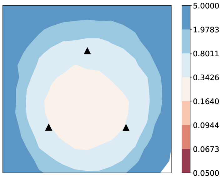
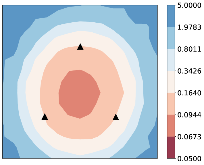
Figure 1: Loss surface of ADM (left) and ADM+SAM (right)

	FID $\downarrow$ (32 $\rightarrow$ 8)	$\|\epsilon_{\theta}\|^{2}$ gap $\downarrow$	LPF $\downarrow$
ADM	34.47 $\overset{\text{{\tiny{\color[rgb]{1,0,0}+13.65}}}}{\longrightarrow}$ 48.02	+11.39	0.097
+SAM	9.01 $\overset{\text{{\tiny{\color[rgb]{0,0.6,0}-0.07}}}}{\longrightarrow}$ 8.94	+3.32	0.063

Table 1: Comparison of the 1) Frechet Inception Distance (FID) scores under 32- and 8-bit precision with (+/-) changes, 2) the gap of $\|\epsilon\|_{2}$ with training, 3) flatness metric called LPF for ADM and +SAM in the CIFAR-10 experiments. $\downarrow$: a lower value is preferred.

(a) ADM

(b) ADM+SAM

Figure 2: Generated samples of 8-bit quantized models for CIFAR-10. Model parameters are directly converted from 32-bit to 8-bit after training, without further optimization or adaptation.

As a preview of our analysis, Figures 1, 2, and Table 1 hint at the role and benefits of the generative models with flat minima. We find that SAM [8], an optimizer designed to promote flatter loss surfaces, significantly enhances flatness when applied to a baseline, i.e., Ablated Diffusion Model (ADM) [7], as shown in Figure 1 and Table 1 (measured using Low-Pass-Filter (LPF) flatness metric [2]). Regarding the benefits from flatness, we observe improved FID, reduced exposure biases (as indicated by the $\|\epsilon\|^{2}$ gap [31]), and lower degradation from model quantization (as reflected in 8-bit precision FID and qualitative results in Figure 2).

Returning to the key question, we set out to investigate the implication of flat loss landscapes in generative models, particularly diffusion models [12]. To make progress, we first seek to refine our core research question: “Why might flatter minima be desirable in generative models, and what theoretical guarantees can we establish?” To address these questions, we conduct a theoretical and empirical analysis of flat minima in diffusion models. First, we establish a theoretical link between the model’s parameter space and data probability density (Theorem 1), showing that flatter minima improve robustness to perturbations in the target prior distribution. As a consequence, we prove that the divergence between the true distribution and the learned distribution is upper-bounded, indicating that flat minima enable diffusion models to generalize not only to the training distribution but also to variations in perturbed data densities (Theorem 2). This insight suggests that flat diffusion models exhibit superior robustness when out-of-distribution is given, demonstrating their ability to cope with error accumulation problem during iterative sampling process, known as exposure bias problem [32, 31, 22]. Moreover, the loss flatness in the parameter space directly implies the robustness against model parameter changes, which indicates that the flatness offers the robustness of generative performance when the model has been quantized.

To complement our theoretical findings, we empirically examine the effects of explicit flatness regularization. Initially, we expect that applying SAM to diffusion models would yield improvements similar to those observed in discriminative settings. However, an intriguing discovery emerges: diffusion models are inherently much flatter than anticipated. Unlike discriminative models, where typical SAM trade-off values significantly impact on flatness, applying standard regularization strengths to diffusion models produced almost no discernible change. Further analysis reveals that diffusion models naturally exhibit a flat loss landscape, likely due to the diverse range of noise levels they are trained to denoise. Building on this observation, we find that significantly stronger regularization is required in diffusion models for SAM to induce meaningful flatness, setting them apart from their discriminative counterparts.

To validate these findings, we conduct extensive experiments on CIFAR-10, LSUN Tower, and FFHQ. Our results show that flat minima in diffusion models consistently improve generative performance with enhanced generalization. This improved generalization offers several practical advantages. For instance, we observe that flat diffusion models better mitigate exposure bias, where errors in noise estimation accumulate over iterations, leading to more stable sampling dynamics. We also show that flat diffusion models results a low quantization error where the model precision is reduced from 32-bit to 8-bit.

We summarize our contributions as follows. Our work provides the first systematic investigation into the role of flat minima in generative models, offering both theoretical insights and practical implications:

• We explore diffusion models through the lens of flat loss landscapes, revealing their inherent flatness.

• We establish a theoretical link between flat minima and generalization, proving that flatness improves robustness via an upper-bound on the divergence between the target and learned distributions.

• We empirically analyze SWA [13] and EMA, showing that while they improve FID, they do not significantly enhance flatness. In contrast, SAM reshapes the loss surface and effectively promotes flatness in diffusion models.

• We demonstrate how these insights address practical challenges in generative modeling through extensive evaluations on CIFAR-10, LSUN Tower, and FFHQ, analyzing FID performance, exposure bias, model quantization error, and loss landscape properties.

2 Preliminaries and Backgrounds

2.1 Optimization for flatness

Algorithm 1 Pseudo algorithm for SWA, EMA, SAM

Input: $w_{0}$: Initial weights, $\rho$: size of perturbation,
$c$: Cycle length, $\lambda$: update momentum
Output: $w,w_{SWA},w_{EMA}$

1: $w,w_{SWA},w_{EMA}\leftarrow w_{0}${Initialize weights with $w_{0}$}

2: for $i=0,...,n-1$ do

3:  if SWA then

4:   $\alpha\leftarrow\alpha(i)$ {Calculate LR for the iteration}

5:  end if

6:  if SAM then

7:   $\hat{w}\leftarrow w+\rho\frac{\nabla\mathcal{L}_{i}(w)}{\|\nabla\mathcal{L}_{i}(w)\|}$ {Ascent step}

8:   $w\leftarrow w-\alpha\nabla\mathcal{L}_{i}(\hat{w})$ {Descent step}

9:  else

10:   $w\leftarrow w-\alpha\nabla\mathcal{L}_{i}(w)$

11:  end if

12:  if SWA & mod($i,c$)=0 then

13:   $n_{models}\leftarrow i/c$ {Number of models}

14:   $w_{SWA}\leftarrow\frac{w_{SWA}\cdot n_{models}+w}{n_{models}+1}$ {Update average}

15:  else if EMA then

16:   $w_{EMA}\leftarrow(1-\lambda)\cdot w_{EMA}+\lambda\cdot w$ {Update average}

17:  end if

18: end for

EMA. EMA is a weight-averaging method that blends a fraction of newly updated parameters with a fraction of previously accumulated parameters at each step. Formally, for parameters $\theta$, the EMA update is: $\theta_{\text{EMA}}\leftarrow(1-\lambda)\theta_{\text{EMA}}+\lambda\,\theta,\quad\lambda\in(0,1).$ Heuristically ensembling different models from multiple iterations reaches flat local minima and improves generalization capacities [10, 16, 24].

SWA. SWA [13] stabilizes training by maintaining an ongoing average of model weights across training epochs. Rather than relying on the final parameters from a single run, SWA updates this average—typically during the latter part of training—leading to an overall smoothing effect in the loss landscape. Although SWA and EMA share the idea of parameter averaging, SWA is directly motivated by the search for flatter minima, which improves generalization.

SAM. SAM [8] is an optimization technique that promotes generalization by steering model parameters toward flatter regions of the loss landscape. It incorporates a sharpness term into the objective, defined as the maximal increase in loss within an $\ell_{2}$-ball of radius $\rho$ around the current parameters $\theta$: $\max_{\|p\|_{2}\leq\rho}\big{[}L(\theta+p)-L(\theta)\big{]}.$ By minimizing this sharpness term alongside the original loss, SAM encourages solutions that are robust to small perturbations in the parameters, thus improving generalization. The pseudocode for SWA, EMA, and SAM is provided in Algorithm 1.

2.2 Score-based Generative Models

Score-based generative models (SGMs) [38, 39, 40, 41] leverage the score function of a data distribution to iteratively generate samples by solving Stochastic Differential Equations (SDEs). Let $p_{\text{data}}(\mathbf{x})$ be the unknown data distribution. The score function is defined as the gradient of the log-density:

$$\nabla_{\mathbf{x}}\log p_{\text{data}}(\mathbf{x}).$$ (1)

Instead of modeling $p_{\text{data}}(\mathbf{x})$ explicitly, SGMs learn a neural network $s_{\theta}(\mathbf{x},t)$ to approximate the score function under slight noise perturbations, $t$ is timestep.

SGMs can be formulated as a stochastic process where noise is gradually added to the data in the forward direction and removed in the backward direction.

Forward SDE. The forward diffusion process is defined by the following SDE:

$$d\mathbf{x}=f(\mathbf{x},t)dt+g(t)d\mathbf{w},$$ (2)

where $f(\mathbf{x},t)$ is the drift coefficient that controls deterministic changes, $g(t)$ is the diffusion coefficient that controls noise intensity, and $d\mathbf{w}$ denotes a standard Wiener process.

Reverse SDE. Using the learned score function, we can reverse the diffusion process to generate new samples. The backward SDE is given by:

$$d\mathbf{x}=\left[f(\mathbf{x},t)-g^{2}(t)\nabla_{\mathbf{x}}\log p_{t}(\mathbf{x})\right]dt+g(t)d\bar{\mathbf{w}},$$ (3)

where $\nabla_{\mathbf{x}}\log p_{t}(\mathbf{x})$ is the time-dependent score function, approximated by $s_{\theta}(\mathbf{x},t)$, and $d\bar{\mathbf{w}}$ is a standard Wiener process running in reverse time. To successfully estimate the score function, score matching objective is defined as:

$$\mathcal{L}_{\text{SGM}}=\mathbb{E}_{t}\left[\lambda(t)\cdot\mathbb{E}_{p_{t}(\mathbf{x})}\left[\left\|s_{\theta}(\mathbf{x},t)-\nabla_{\mathbf{x}_{t}}\log p_{t}(\mathbf{x})\right\|_{2}^{2}\right]\right].$$ (4)

2.3 Diffusion models

SGMs are closely related to diffusion probabilistic models (DPMs) [37, 12], which DPMs can be viewed as a discrete-time approximation of SGM with following forward diffusion process:

$$q(\mathbf{x}_{t}|\mathbf{x}_{t-1}):=\mathcal{N}(\mathbf{x}_{t};\sqrt{1-\beta_{t}}\mathbf{x}_{t-1},\beta_{t}\mathbf{I}),$$ (5)

where $\beta_{t}$ is a predefined parameter by variance scheduling, $\mathcal{N}(m;\sigma^{2})$ is a Guassian distribution with mean $m$ and variance $\sigma^{2}$, and $\mathbf{I}$ is an identity matrix. Given an initial sample $\mathbf{x}_{0}$, the noisy sample at timestep $t$ is generated as follows:

$$\mathbf{x}_{t}=\sqrt{\bar{\alpha}_{t}}\mathbf{x}_{0}+\sqrt{1-\bar{\alpha}_{t}}\epsilon_{t},\quad\epsilon_{t}\sim\mathcal{N}(0,\mathbf{I})$$ (6)

where $\alpha_{t}:=1-\beta_{t}$ and $\bar{\alpha}_{t}:=\prod_{s=1}^{t}\alpha_{s}$.

Then, we can analytically derive the posterior distribution of injected gaussian noise as follows:

$$q(\mathbf{x}_{t-1}|\mathbf{x}_{t}) =\mathcal{N}(\mathbf{x}_{t-1};\tilde{\mu}(\mathbf{x}_{t},\mathbf{x}_{0}),\tilde{\beta}_{t}\mathbf{I}),$$ (7)

$$\tilde{\mu}(\mathbf{x}_{t},\mathbf{x}_{0}) =\frac{\sqrt{\bar{\alpha}_{t-1}}\beta_{t}}{1-\bar{\alpha}_{t}}\mathbf{x}_{0}+\frac{\sqrt{\alpha_{t}}(1-\bar{\alpha}_{t-1})}{1-\bar{\alpha}_{t}}\mathbf{x}_{t},$$ (8)

$$\tilde{\beta}_{t} =\frac{1-\bar{\alpha}_{t-1}}{1-\bar{\alpha}_{t}}\beta_{t}$$ (9)

To estimate the posterior distribution, diffusion models parameterize $\tilde{\mu}(\mathbf{x}_{t},\mathbf{x}_{0})$ or instead $\epsilon_{t}$ after applying reparameterization trick. Once trainig is over, diffusion model produce the clean images by iteratively removing the gaussian noise as follows:

$$\mathbf{x}_{t-1}=\frac{1}{\sqrt{\alpha_{t}}}(\mathbf{x}_{t}-\frac{1-\alpha_{t}}{\sqrt{1-\bar{\alpha}_{t}}}\epsilon_{\theta}(\mathbf{x}_{t},t))+\beta_{t}\mathbf{z},.$$ (10)

where $\mathbf{z}\sim\mathcal{N}(0,\mathbf{I})$.

While these iterative denoising frameworks successfully learn the underlying distribution and synthesize images with exceptional fidelity, previous works [32, 31, 22] have raised an input discrepancy problem between the training and sampling phases, known as exposure bias problem. Specifically, during training, the diffusion model is provided with ground truth noisy images (Equation (6)), whereas during sampling, it receives a denoised image (Equation (10)) came from the previous timestep. The presence of errors in these inputs makes it challenging for the diffusion model to accurately predict noise. As these errors accumulate over iterative timesteps, they cause the generated samples to significantly deviate from the desired trajectory.

3 Theoretical Analysis on Flatness

We here theoretically analyze the effect of flat minima in SGMs, with an emphasis on diffusion models.

3.1 Notations

Our analysis is built upon the settings of SGM, which is a fundamental form of diffusion models. Beyond the brief preliminaries in Section 2.2, we introduce additional notations and formulations to be used in our analysis. By following [23], we formulate the score model $s_{\boldsymbol{\theta}}(\cdot,\cdot)$ as a random feature model:

$$s_{\boldsymbol{\theta}}(\mathbf{x},t):=\frac{1}{m}\mathbf{\boldsymbol{\theta}}\sigma\big{(}\mathbf{W}^{T}\mathbf{x}+\mathbf{U}^{T}\mathbf{e}_{t}\big{)},$$ (11)

where $\mathbf{x}\in\mathbb{R}^{d\times 1}$ is the given input, $\mathbf{e}_{t}$ is the timestep embedding for $t$, a group of parameters includes $\boldsymbol{\theta}\in\mathbb{R}^{d\times m}$, $\mathbf{W}\in\mathbb{R}^{d\times m}$ and $\mathbf{U}\in\mathbb{R}^{d_{e}\times m}$, and a few positive integers include $d$, $m$, and $d_{e}$. By following the training procedures of diffusion models, $\boldsymbol{\theta}$ is the learnable parameter, while others, i.e., $\mathbf{W}$ and $\mathbf{U}$, which respectively embed $\mathbf{x}$ and $\mathbf{e}_{t}$, are set to be frozen. For a given timestep $t$, the score matching loss objective defined in Equation 4

$$\mathcal{L}(\mathbf{x};\boldsymbol{\theta},t,p_{t}):=\|s_{\boldsymbol{\theta}}(\mathbf{x},t)-\nabla_{\mathbf{x}}\log{p_{t}(\mathbf{x})}\|_{2}^{2},$$ (12)

where $p_{t}(\mathbf{x})$ is the probability density function for the prior distribution of $\mathbf{x}$.

3.2 Mathematical Claims

For the main claims, we follow the formulation of Equation (12), while omitting timestep $t$ without loss of generality. Our mathematical claims are valid for all timesteps. We start from defining flat minima in SGMs (Definition 1), and the robustness against the gap of ground truth prior $p(\mathbf{x})$ and the estimated prior $\hat{p}(\mathbf{x})$ (Definition 2). For the flat minima definition, we rehearse the definition of flat minima for the supervised learning case [36], thus $\Delta$-flat minima of SGMs with the score matching loss is defined as follows:

Definition 1.

($\Delta$-flat minima) Let us consider a SGM with loss function $\mathcal{L}(\mathbf{x};\boldsymbol{\theta},p)$. A minimum $\boldsymbol{\theta^{*}}$ is $\Delta$-flat minima when the following constraints are hold:

$$\forall\>\delta\in\mathbb{R}^{d\times m}\text{ s.t. }\|\delta\|_{2}\leq\Delta,\>\>\mathcal{L}(\mathbf{x};\boldsymbol{\theta}^{*}+\delta,p)=l^{*}$$

$$\exists\>\delta\in\mathbb{R}^{d\times m}\text{ s.t. }\|\delta\|_{2}>\Delta,\>\>\mathcal{L}(\mathbf{x};\boldsymbol{\theta}^{*}+\delta,p)>l^{*},$$

where $l^{*}:=\mathcal{L}(\mathbf{x};\boldsymbol{\theta}^{*},p)$ and $\Delta\in\mathbb{R}^{+}$.

To extend to robustness against the erroneous estimation of prior probability, we further define the $\mathcal{E}$-distribution gap robustness of SGMs, where $\mathcal{E}$ indicates the divergence between the ground truth $p$ and the estimated $\hat{p}$:

Definition 2.

($\mathcal{E}$-distribution gap robustness) A minimum $\boldsymbol{\theta^{*}}$ is $\mathcal{E}$-distribution gap robust when the following constraints are hold:

$$\forall\>\hat{p}(\mathbf{x})\text{ s.t. }D(p||\hat{p})\leq\mathcal{E},\>\>\mathcal{L}(\mathbf{x};\boldsymbol{\theta}^{*},\hat{p})=l^{*}$$

$$\exists\>\hat{p}(\mathbf{x})\text{ s.t. }D(p||\hat{p})>\mathcal{E},\>\>\mathcal{L}(\mathbf{x};\boldsymbol{\theta}^{*},\hat{p})>l^{*},$$

where $D(\cdot||\cdot)$ is the divergence between two probability density functions, $\hat{p}$ is the perturbed prior distribution of $\mathbf{x}$, and $\mathcal{E}$ is a positive real number.

Let us then bridge the flatness and the robustness. First, based on the definitions of flat minima (Definition 1) and distributional gap robustness (Definition 2), we try to formulate how the perturbation of the parameter, i.e., $\boldsymbol{\theta}+\delta$, links to the perturbed prior distribution $\hat{p}$, with the given equality as follows:

$$\mathcal{L}(\mathbf{x};\boldsymbol{\theta}+\delta,p)=\mathcal{L}(\mathbf{x};\boldsymbol{\theta},\hat{p}).$$ (13)

This means how the parameter perturbation is translated into the shift of the prior, while keeping the loss unchanged. Let us provide a mathematical claim of it:

Theorem 1.

(A perturbed distribution) For a given prior distribution of $p(\mathbf{x})$ and the $\delta$-perturbed minimum, i.e., $\boldsymbol{\theta}+\delta$, the following $\hat{p}(\mathbf{x})$ satisfies the equality (13):

$$\hat{p}(\mathbf{x})=e^{-I(\mathbf{x},\delta)}p(\mathbf{x}),$$ (14)

where $I(\mathbf{x},\delta):=\frac{1}{2}\mathbf{x}^{T}(\delta\mathbf{W}^{T})\mathbf{x}+\mathbf{x}^{T}\delta(\mathbf{U}^{T}\mathbf{e})+C$, and $C\in\mathbb{R}$ is set to satisfy $\displaystyle\int_{\mathbb{R}^{d}}e^{-I(\mathbf{x},\delta)}p(\mathbf{x})d\mathbf{x}=1$.

This theorem shows that the parameter perturbation can be translated into the “scaling” of probability density function. However, the scaling depends on various parameters, thus it is nontrival to imagine the behavior of $\hat{p}$. Let us narrow our view to the diffusion model, where it predicts a noise signal sampled from Gaussian distribution, i.e., $\mathcal{N}(0,\mathbf{I})$. It changes our focus on handling the noise distribution, i.e., $\epsilon$, rather than the distribution of data side, i.e., $p$. The following corollary describes how the perturbed $\hat{\epsilon}$ looks like:

Corollary 1.

(Diffusion version of Theorem 1) For a given prior Gaussian distribution of noise $\epsilon\sim\mathcal{N}(0,\mathbf{I})$ and the $\delta$-perturbed minimum, i.e., $\boldsymbol{\theta}+\delta$, the following $\hat{\epsilon}$ satisfies the equality (13):

$$\hat{\epsilon}=e^{-I(\mathbf{x},\delta)}\epsilon=\mathcal{N}(\boldsymbol{\mu}_{\delta},\Sigma_{\delta}),$$ (15)

where $\Sigma_{\delta}:=\bigg{(}\mathbf{I}+\displaystyle\frac{\delta_{w}}{m}\bigg{)}^{-1}$, $\boldsymbol{\mu}_{\delta}:=\displaystyle\frac{1}{m}\Sigma_{\delta}\delta_{u}$.

Remark 1.

($\hat{\epsilon}$ becomes perturbed Gaussian) For the diffusion models, we emphasize that the perturbation in the parameter space, $\delta$, leads to the perturbation of distribution, which follows the Gaussian distribution.

Next, let us consider all possible perturbations within the ball of norm, i.e., $\|\Delta\|_{2}\leq\Delta$. The resulting set of perturbed distributions induced by the parameter perturbation is defined as follows:

Definition 3.

(A set of perturbed distribution) For a given distribution of $p(\mathbf{x})$, a set of distributions $\hat{\mathcal{P}}(\mathbf{x};p,\Delta)$ is defined as the set of perturbed distributions $\hat{p}(\mathbf{x})$:

$$\hat{\mathcal{P}}(\mathbf{x};p,\Delta):=\{e^{-I(\mathbf{x},\delta)}p(\mathbf{x})\>|\>\|\delta\|_{2}\leq\Delta\}.$$ (16)

From the definition, $\Delta$-flat minimum flattens all loss values of the perturbed parameters. Consequently, the flat minimum achieves flat loss values for all possible distributions within $\hat{\mathcal{P}}$, as formally shown in the following proposition:

Proposition 1.

(A link from $\Delta$-flatness to $\hat{\mathcal{P}}$) A $\Delta$-flat minimum $\boldsymbol{\theta}^{*}$ achieves the flat loss values for all distributions sampled from the set of perturbed distribution:

$$\forall\>p\sim\hat{\mathcal{P}}(\mathbf{x};p,\Delta),\>\>\mathcal{L}(\mathbf{x};\boldsymbol{\theta}^{*},p)=l^{*}$$ (17)

$$\exists\>p\nsim\hat{\mathcal{P}}(\mathbf{x};p,\Delta),\>\>\mathcal{L}(\mathbf{x};\boldsymbol{\theta}^{*},p)>l^{*}.$$ (18)

We finally link flatness to the distributional gap, i.e., connecting Definitions 1 and 2. Let us anticipate the distribution in $\hat{\mathcal{P}}$ with the maximal divergence from $p$. The distribution gap $\mathcal{E}$ is then upper bounded by the divergence of the most outreached distribution:

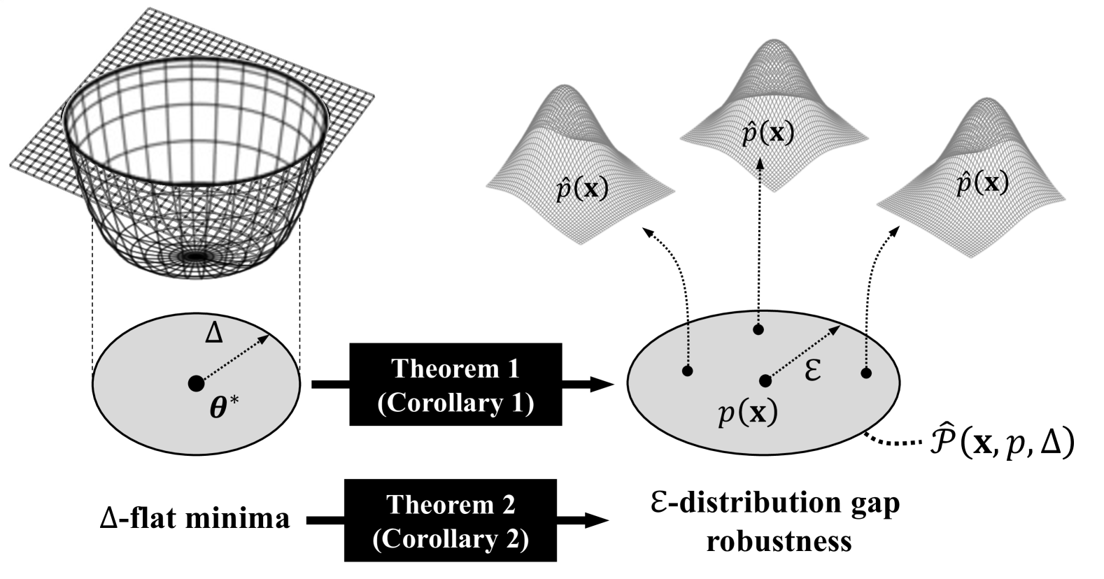
Figure 3: A conceptual illustration of theoretical analysis. Theorem 1 (Corollary 1 for diffusion model) translates the perturbation in the parameter space into the set of perturbed distributions. Theorem 2 (Corollary 2 for diffusion model) shows that flat minima leads to the robustness against the distribution gap.

FID Score	Dataset	CIFAR-10 (32x32)		LSUN Tower (64x64)		FFHQ (64x64)
	$T^{\prime}$	20 steps	100 steps	20 steps	100 steps	20 steps	100 steps
Algorithms	ADM	34.47	8.80	36.65	8.57	30.81	7.53
	+EMA	10.63	4.06	7.87	2.49	19.03	6.19
	+SWA	11.00	3.78	8.72	2.31	17.93	5.49
	+SAM	9.01	3.83	16.02	4.79	31.89	12.43
	+SAM+EMA	7.00	3.18	6.66	2.30	21.48	6.44
	+SAM+SWA	7.27	2.96	6.50	2.27	21.11	5.32

Table 2: FID Scores for ADM baselines with different algorithms on CIRAR-10, LSUN Tower, and FFHQ dataset. We use DDPM sampling with shorter respacing timesteps, $T^{\prime}=20,100$.

Theorem 2.

(A link from $\Delta$-flatness to $\mathcal{E}$-gap robustness) A $\Delta$-flat minimum achieves $\mathcal{E}$-distribution gap robustness, such that $\mathcal{E}$ is upper-bounded as follows:

$$\mathcal{E}\leq\operatorname*{arg\,max}_{\hat{p}\sim\hat{\mathcal{P}}(\mathbf{x};p,\Delta)}D(p||\hat{p}).$$ (19)

Let us further manipulate the upper bound for the diffusion model case. From Corollary 1, $\hat{p}$ is a form of Gaussian distribution; thus it is possible to achieve the closed form of the upperbound as follows:

Corollary 2.

(Diffusion version of Theorem 2) For a diffusion model, a $\Delta$-flat minimum achieves $\mathcal{E}$-distribution gap robustness, such that $\mathcal{E}$ is upper-bounded as follows:

$$\mathcal{E} \leq\operatorname*{arg\,max}_{\|\delta\|_{2}\leq\Delta}\frac{1}{2}\Bigg{[}\log|\Sigma_{\delta}|-d+tr(\Sigma_{\delta}^{-1})+{\boldsymbol{\mu}_{\delta}}^{T}{\Sigma_{\delta}}^{-1}\boldsymbol{\mu}_{\delta}\Bigg{]}$$

$$\leq\frac{1}{2}\Bigg{[}\sum_{i=1}^{d}\log\frac{m}{m+\sigma_{i}}+\sum_{i=1}^{d}\frac{\sigma_{i}}{m}+\frac{\sigma_{d}}{m^{2}}\|\mathbf{U}^{T}\mathbf{e}\|_{2}^{2}\Delta^{2}\Bigg{]},$$ (20)

where $\sigma_{i}$ is an eigenvalue of $\Sigma_{\delta}^{-1}$ with the increasing order of $\sigma_{1}\,\leq\,\sigma_{2}\,\leq\,\dots\,\leq\,\sigma_{d}$.

Remark 2.

(Flatter minima enhance distribution gap robustness) It is noteworthy that flatter minima with a large $\Delta$ flatten the loss values for the far-pushed away perturbed distribution $\hat{p}$ with large divergence, leading to the larger bound of $\mathcal{E}$. It indicates that flattening the loss surface makes the generative model zero-force the loss values of diversified prior distribution, thus enhancing the robustness against the prior distribution gap. On the other hand, $m$ is the number of trainable parameters, which is quite large, so that the first and second terms are negligible.

Flatness reduces exposure bias (a gap of $\hat{\epsilon}$ and $\epsilon$): A clear advantage of flatness is robustness to exposure bias, where the errors in noise estimation accumulate over iterations, thus severely deteriorates the generative performance. In formula, $\hat{\epsilon}$ deviates from $\epsilon$. We argue that a generative model with a flat minimum suppresses the loss values of perturbed estimation, so that the error accumulation is sufficiently relieved. To be shown in experiments, we empirically confirm that flat minima tend to show a smaller exposure bias, leading to the robust generative performance.

Flatness becomes robust to model quantization (a compression from $\boldsymbol{\theta}$ to $\hat{\boldsymbol{\theta}}$): For another benefit, flat minima make the model robust to the performance degradation caused by the model quantization. Recently, quantization of generative models becomes crucial, when enabling real-time applications of generative tasks [44, 26, 27]. We claim that flat minima inherently bolster the robustness against the degradation due to the quantization, because the quantized model, $\hat{\boldsymbol{\theta}}$, can be viewed as a perturbed version of the full-precision parameter, i.e., $\hat{\boldsymbol{\theta}}=\boldsymbol{\theta}+\Delta$; thus the loss remains flat for the perturbation [27]. In experiments, we clearly demonstrate that the diffusion model with flatness is remarkably resilient to the degradation from quantization than other methods.

A conceptual overview of our theoretical analysis is illustrated in Figure 3. The proof of Theorem 1, and Corollary 1, 2 are given in Appendix 1 in Supplementary.

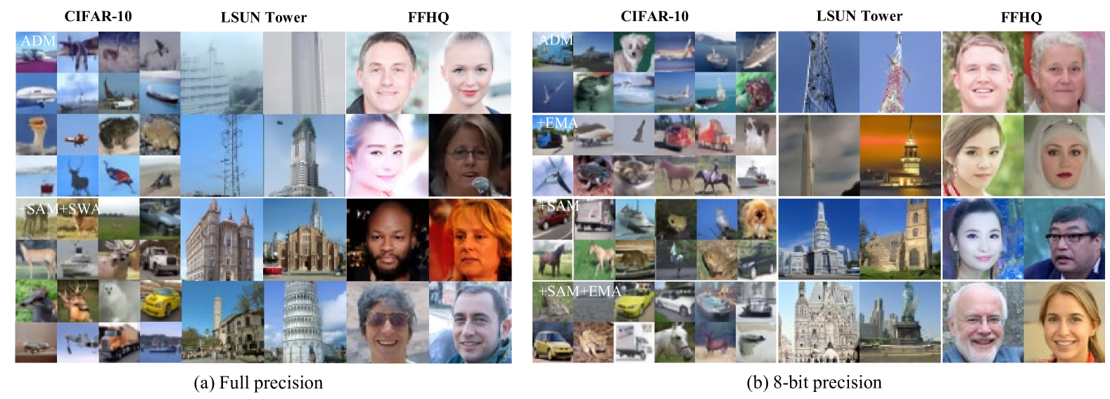
Figure 4: Generation results of (a) full precision (32-bit) and (b) 8-bit quantized models. We use respaced timesteps $T^{\prime}=20$ for sampling. For the 8-bit case, we selectively compare +EMA, +SAM and their combinations, where the relatively flatter minima have been found.

4 Experiments

4.1 Experiments Settings

Datasets. Similar to the setup in [32], we use CIFAR-10 (32x32), LSUN-tower (64x64), and FFHQ (64x64).

Baselines. We use ADM baselines [7] for training unconditional DDPM. We incorporate flatness-enhancing approaches such as SWA [8] and SAM [8] to deliberately enhance flatness and reveal the effects of that. Because EMA may influence flatness [16], we distinguish between baselines with and without EMA. Additionally, we compare DDPM-IP [32] that introduces input perturbation during training to encourage smoothness in the diffusion model.

Experimental details. We trained the model for 200K steps on the CIFAR-10 and LSUN Tower datasets, and 120K steps on the FFHQ dataset. We employed the Adam optimizer for all experiments with a learning rate of $1e^{-}{4}$, following  [7, 30]. For +IP, we used an input perturbation strength of 0.1 following [32], and for SWA, we set the cycle length $c$ to 100 and start averaging from 180K steps for CIFAR-10 and LSUN Tower datasets. Finally, for +SAM, we tuned the $\rho\in[1e^{-1},1e^{-2},1e^{-3}]$ parameters.

Evaluation metrics. We evaluate generative performance by comparing Fréchet Inception Distance (FID) scores [11] using subsequence of timesteps $(T^{\prime}<T)$. We assess Low-Pass Filter (LPF) [2] values and loss plots under perturbation [5] to determine whether the baselines successfully identify a flat loss surface. To further investigate generalization ability of diffusion models, we investigate exposure bias and quantization error. For exposure bias [31], we compare the square norm of the predicted noise, $\left\|\epsilon_{\theta}\right\|^{2}$ when models are conditioned on ground truth noisy images during training versus when they receive error-contained inputs at different sampling timesteps [30]. For quantization error, we compare the FID before and after quantization.

4.2 Generative Performance

The quantitative and qualitative results presented in Table. 2 and Figure. 4 demonstrate the generative performance of baselines. From Table. 2, we observe that applying EMA consistently improves FID scores across all datasets and respaced timesteps, demonstrating its effectiveness in stabilizing model updates and enhancing sample quality. SWA also provides notable improvements but does not outperform EMA in most cases. The introduction of SAM, however, leads to the lowest FID scores, particularly in the +SAM+SWA setting, suggesting that explicitly controlling flatness results in a more robust and generalizable generative model. The trend is particularly evident in the 100-step respacing setting, where SAM-based models consistently outperform baselines, indicating that flat minima contribute to better sample quality, especially under reduced sampling steps. Figure. 4 further supports these findings by providing visual comparisons of generated images.

LPF $\downarrow$	w/o	+EMA	+SWA
ADM	0.097	0.099	0.099
+IP	0.103	0.101	0.102
+SAM	0.063	0.063	0.063

$\downarrow$: a lower value is preferred.

Table 3: Flatness measure on CIFAR-10. We calculate the loss with the perturbed model with Gaussian noise. Lower values indicate a flatter loss landscape.

4.3 Flatness Measurement

In Table. 3, we compare LPF flatness measures [2], where lower values indicate a flatter loss landscape. We observe that ADM already possesses a certain level of flatness. Interestingly, we find that ensemble-like averaging, such as +SWA and +EMA, fail to induce additional flatness. In contrast, +SAM finds a flatter loss surface by explicitly perturbing model weights, as evidenced by SAM-applied models consistently achieving the lowest LPF values and significantly superior performance to other baselines. Also, we plot another measurement to support these findings further. Figure. 5 shows how the loss value increases as the model perturbation is imposed for CIFAR-10. +IP, +EMA, and +SWA show no significant differences, coincide with the result of LPF, where these fail to find additional flatness. In this setting, +SAM shows a flatter behavior than other algorithms. It shows that diffusion models already show flatter loss landscapes, and ensemble-like averaging, such as +SWA and EMA, shows less impact. Moreover, finding flat minima explicitly leads to the flatness in diffusion models. We provide plots for other algorithms, including +IP+EMA, +IP+SWA, +SAM+EMA, +SAM+SWA, in the Appendix.

4.4 Flat Diffusion Models are Robust

We show that flat diffusion models perform well under input shifts. As an instantiation, we set two cases: 1) exposure bias and 2) quantization error. Both scenarios share the common characteristic that diffusion models receive error-accumulated inputs, leading to performance degradation.

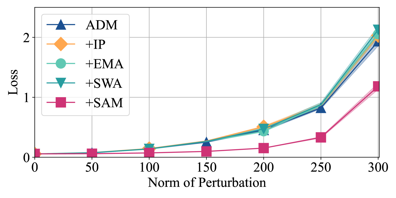
Figure 5: Loss plots under perturbation for CIFAR-10. As the norm of model perturbation increases, we plot the corresponding loss values. A smaller slope indicates a flatter loss landscape.

Exposure bias. In Figure. 6, we compare the L2 norm of the predicted noise in diffusion models. A model that closely aligns with the training trajectory is expected to exhibit lower exposure bias, thereby mitigating distribution shifts over iterative sampling steps. We observe that SAM-applied models consistently maintain L2 norms closer to the training curve, indicating a lower degree of exposure bias. This result aligns well with their superior FID performance reported in Table. 2, suggesting that flat diffusion models generalize better across sampling timesteps and effectively combat error accumulation.

Model quantazation error. Table. 4 presents the FID scores of quantization across baselines, when reducing precision from 32-bit to 8-bit. Here, we quantize model parameters to 8-bit values using scaling and rounding, without any additional fine-tuning or retraining. Thanks to +SAM that aims to the robustness of model perturbation, flatter diffusion models results in surprisingly better robustness under quantization. These findings also support that +SAM is robust to model quantization.

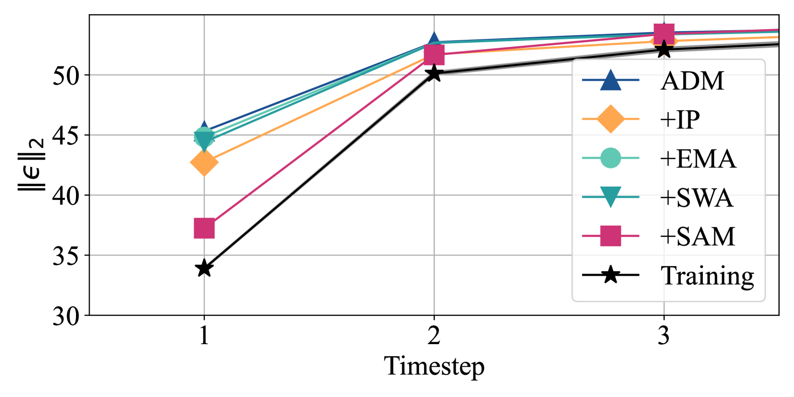
Figure 6: L2 norm of the predicted noise for CIFAR-10. As the gap with “Training” decreases, the predicted noise norm during sampling approaches the ground truth.

5 Related works

Diffusion models. Diffusion probabilistic models (DPMs) [12, 7, 38, 39, 41] have been recently emerged as powerful generative frameworks, achieving state-of-the-art performance in image [35, 33] and video [15, 3] synthesis. Despite extensive research on improving diffusion models through architecture modifications [29, 14, 33], enhanced training strategies [43], and novel noise scheduling techniques [41, 42], relatively little attention has been given to understanding their loss landscape properties.

Flat minima in various tasks. Flat minima have garnered significant attention in classification and domain generalization tasks with the view of loss landscape  [13, 9, 21] and objective function [8, 17]. Other tasks also adopt the flatness for their performance. In federated learning, for example, where client devices collect and train on heterogeneous datasets, ensuring robust generalization across diverse data distributions is a core challenge. Recent works such as [34, 4, 20] have employed flat minima strategies to mitigate this data heterogeneity issue by obtaining the model robust to distribution shift. Some findings encouraging flat reward in RL leads to learning of robust policies [19, 18].

Flat minima on diffusion models. Recent empirical findings suggest that diffusion models inherently exhibit flatter loss landscape [45]. This observation aligns with the broader literature on the benefits of flat minima, particularly in supervised learning, where flatter loss surfaces are known to enhance generalization and improve robustness to perturbations. However, the implications of flat minima in the context of diffusion models remain largely unexplored. While some prior works have attempted to leverage smooth function properties to improve generative modeling [1, 6, 32], they primarily focus on enforcing Lipschitz continuity or reducing gradient penalties rather than explicitly studying the role of flatness in diffusion models. To the best of our knowledge, no prior research has systematically investigated how flat minima influence diffusion models, how they impact generative performance, or whether they can be intentionally optimized to enhance diffusion model robustness. This gap in understanding motivates us, where we aim to establish a theoretical and empirical foundation for analyzing the effect of flat minima on diffusion models.

32-bit $\rightarrow$ 8-bit	20 steps	100 steps
ADM	34.47 $\overset{\text{{\tiny{\color[rgb]{1,0,0}+13.65}}}}{\longrightarrow}$ 48.02	8.80 $\overset{\text{{\tiny{\color[rgb]{1,0,0}+3.98}}}}{\longrightarrow}$ 12.78
+EMA	10.63 $\overset{\text{{\tiny{\color[rgb]{1,0,0}+10.02}}}}{\longrightarrow}$ 20.65	4.06 $\overset{\text{{\tiny{\color[rgb]{1,0,0}+3.3}}}}{\longrightarrow}$ 7.36
+SAM	9.01 $\overset{\text{{\tiny{\color[rgb]{0,0.6,0}-0.07}}}}{\longrightarrow}$ 8.94	3.83 $\overset{\text{{\tiny{\color[rgb]{1,0,0}+0.19}}}}{\longrightarrow}$ 4.02
+SAM+EMA	7.00 $\overset{\text{{\tiny{\color[rgb]{1,0,0}+0.2}}}}{\longrightarrow}$ 7.20	3.18 $\overset{\text{{\tiny{\color[rgb]{0,0.6,0}-0.06}}}}{\longrightarrow}$ 3.12

Table 4: FID performance on CIFAR-10 when model parameters are quantized to 8-bit. We apply direct quantization by clipping and rounding 32-bit parameters without additional fine-tuning. The 32-bit performance results are identical to those in Table. 2.

6 Conclusion

We presented an in-depth investigation of the role and benefits of flat loss surfaces in generative models, which have remained unknown despite the great success of deep generative models. Our study explored this unknown by analyzing how flatness influences generative modeling and demonstrating its possible impact on robustness. First, our theoretical analysis reveals that the loss flatness of the generative models enhances the robustness against the disruptions of the target data distributions or the perturbations of model parameters. These insights naturally link to the reduced exposure bias problem and the model quantization error. Based on the evaluations on CIFAR-10, LSUN Tower, and FFHQ, we demonstrated that 1) SAM is suitable to seek flatter minima of diffusion models rather than SWA and EMA, 2) flat minima reduce exposure bias with a minimal gap between testing and training, and 3) a flat model keeps its generative performance even with a strong model quantization; coinciding with our theory.

Supplementary material

Appendix A Mathematical claims and proofs

For the main claims, we follow $\mathcal{L}(\mathbf{x};\boldsymbol{\theta},t,p_{t}):=||s_{\boldsymbol{\theta}}(\mathbf{x},t)-\nabla_{\mathbf{x}}\log{p_{t}(\mathbf{x})}||_{2}^{2}$, while dropping the timestep $t$ without loss of generality. Our mathematical claims are valid for all timesteps.

Definition 1. ($\Delta$-flat minima) Let us consider a SGM with loss function $\mathcal{L}(\mathbf{x};\boldsymbol{\theta},p)$. A minimum $\boldsymbol{\theta^{*}}$ is $\Delta$-flat minima when the following constraints are hold:

$$\forall\>\delta\in\mathbb{R}^{d\times m}\text{ s.t. }\|\delta\|_{2}\leq\Delta,\>\>\mathcal{L}(\mathbf{x};\boldsymbol{\theta}^{*}+\delta,p)=l^{*}$$

$$\exists\>\delta\in\mathbb{R}^{d\times m}\text{ s.t. }\|\delta\|_{2}>\Delta,\>\>\mathcal{L}(\mathbf{x};\boldsymbol{\theta}^{*}+\delta,p)>l^{*},$$

where $l^{*}:=\mathcal{L}(\mathbf{x};\boldsymbol{\theta}^{*},p)$ and $\Delta\in\mathbb{R}^{+}$.

Definition 2. ($\mathcal{E}$-distribution gap robustness) A minimum $\boldsymbol{\theta^{*}}$ is $\mathcal{E}$-distribution gap robust when the following constraints are hold:

$$\forall\>\hat{p}(\mathbf{x})\text{ s.t. }D(p||\hat{p})\leq\mathcal{E},\>\>\mathcal{L}(\mathbf{x};\boldsymbol{\theta}^{*},\hat{p})=l^{*}$$

$$\exists\>\hat{p}(\mathbf{x})\text{ s.t. }D(p||\hat{p})>\mathcal{E},\>\>\mathcal{L}(\mathbf{x};\boldsymbol{\theta}^{*},\hat{p})>l^{*},$$

where $D(\cdot||\cdot)$ is the divergence between two probability density functions, $\hat{p}$ is the perturbed prior distribution of $\mathbf{x}$, and $\mathcal{E}$ is a positive real number.

Theorem 1. (A perturbed distribution) For a given prior distribution of $p(\mathbf{x})$ and the $\delta$-perturbed minimum, i.e., $\boldsymbol{\theta}+\delta$, the following $\hat{p}(\mathbf{x})$ satisfies the $\mathcal{L}(\mathbf{x};\boldsymbol{\theta}+\delta,p)=\mathcal{L}(\mathbf{x};\boldsymbol{\theta},\hat{p})$:

$$\hat{p}(\mathbf{x})=e^{-I(\mathbf{x},\delta)}p(\mathbf{x}),$$ (21)

where $I(\mathbf{x},\delta):=\frac{1}{2}\mathbf{x}^{T}(\delta\mathbf{W}^{T})\mathbf{x}+\mathbf{x}^{T}\delta(\mathbf{U}^{T}\mathbf{e})+C$, and $C\in\mathbb{R}$ is set to satisfy $\displaystyle\int_{\mathbb{R}^{d}}e^{-I(\mathbf{x},\delta)}p(\mathbf{x})d\mathbf{x}=1$.

Proof.

By following [23], we formulate the score model $s_{\boldsymbol{\theta}}(\cdot,\cdot)$ as a random feature model:

$$s_{\boldsymbol{\theta}}(\mathbf{x},t):=\frac{1}{m}\boldsymbol{\theta}\sigma(\mathbf{W}^{T}\mathbf{x}+\mathbf{U}^{T}\mathbf{e}_{t})$$ (22)

where $\mathbf{x}\in\mathbb{R}^{d\times 1}$, $\boldsymbol{\theta}\in\mathbb{R}^{d\times m}$, $\mathbf{W}\in\mathbb{R}^{d\times m}$, $\mathbf{U}\in\mathbb{R}^{d_{e}\times m}$, $\mathbf{e}_{t}\in\mathbb{R}^{d_{e}\times 1}$, and $d$, $m$, $d_{e}$ are positive integers.

The score matching loss objective is defined as

$$\mathcal{L}(\mathbf{x};\boldsymbol{\theta},p):=||s_{\boldsymbol{\theta}}(\mathbf{x})-\nabla_{\mathbf{x}}\log{p(\mathbf{x})}||_{2}^{2},$$ (23)

For the perturbation $\delta\in\mathbb{R}^{d\times m}$ in the diffusion model parameters $\boldsymbol{\theta}$, the perturbed loss value becomes:

$$\mathcal{L}(\mathbf{x};\boldsymbol{\theta}+\delta,p):=||s_{\boldsymbol{\theta}+\delta}(\mathbf{x})-\nabla_{\mathbf{x}}\log{p(\mathbf{x})}||_{2}^{2}.$$ (24)

$$s_{\boldsymbol{\theta}+\delta}(\mathbf{x})-\nabla_{\mathbf{x}}\log{p(\mathbf{x})}$$ (25)

$$=\frac{1}{m}(\boldsymbol{\theta}+\delta)\sigma(\mathbf{W}^{T}\mathbf{x}+\mathbf{U}^{T}\mathbf{e})-\nabla_{\mathbf{x}}\log{p(\mathbf{x})}$$ (26)

$$=\frac{1}{m}\boldsymbol{\theta}\sigma(\mathbf{W}^{T}\mathbf{x}+\mathbf{U}^{T}\mathbf{e})+\frac{1}{m}\delta\sigma(\mathbf{W}^{T}\mathbf{x}+\mathbf{U}^{T}\mathbf{e})-\nabla_{\mathbf{x}}\log{p(\mathbf{x})}$$ (27)

Let us focus on the second and third terms with the assumptions of the positive outputs for the activation function:

$$\frac{1}{m}\delta(\mathbf{W}^{T}\mathbf{x}+\mathbf{U}^{T}\mathbf{e})-\nabla_{\mathbf{x}}\log{p(\mathbf{x})}$$ (28)

Here, let us define $I(\mathbf{x})$ as a function of $\mathbf{x}$, whose derivative is the first term of the previous equation:

$$\frac{\partial I(\mathbf{x})}{\partial\mathbf{x}}=\frac{1}{m}\delta(\mathbf{W}^{T}\mathbf{x}+\mathbf{U}^{T}\mathbf{e})$$ (29)

Based on it, $I(\mathbf{x})\in\mathbb{R}$ is

$$I(\mathbf{x})=\frac{1}{2}\mathbf{x}^{T}(\delta\mathbf{W}^{T})\mathbf{x}+\mathbf{x}^{T}\delta(\mathbf{U}^{T}\mathbf{e})+C,$$ (30)

with the assumption $\delta\mathbf{W}^{T}$ is symmetric and where $C$ is a constant real number.

$$\frac{1}{m}\delta(\mathbf{W}^{T}\mathbf{x}+\mathbf{U}^{T}\mathbf{e})-\nabla_{\mathbf{x}}\log{p(\mathbf{x})}$$ (31)

$$=\nabla_{\mathbf{x}}I(\mathbf{x})-\nabla_{\mathbf{x}}\log{p(\mathbf{x})}$$ (32)

$$=-\nabla\log{\Big{(}e^{-I(\mathbf{x})}p(\mathbf{x})\Big{)}}$$ (33)

When $C$ is the real number that satisfies the following condition for the function $I$ with $C$:

$$\int_{\mathbb{R}^{d}}e^{-I(\mathbf{x})}p(\mathbf{x})=1,$$ (34)

then we can define $\hat{p}(\mathbf{x})$ to be a perturbed PDF of inputs:

$$\hat{p}(\mathbf{x}):=e^{-I(\mathbf{x})}p(\mathbf{x})$$ (35)

$$=\exp{\Big{\{}-\frac{1}{2m}\mathbf{x}^{T}(\delta\mathbf{W}^{T})\mathbf{x}-\frac{1}{m}\mathbf{x}^{T}\delta(\mathbf{U}^{T}\mathbf{e})-C^{*})\Big{\}}}p(\mathbf{x})$$ (36)

∎

Corollary 1. (Diffusion version of Theorem 1) For a given prior Gaussian distribution of noise $\epsilon\sim\mathcal{N}(0,\mathbf{I})$ and the $\delta$-perturbed minimum, i.e., $\boldsymbol{\theta}+\delta$, the following $\hat{\epsilon}$ satisfies the $\mathcal{L}(\mathbf{x};\boldsymbol{\theta}+\delta,p)=\mathcal{L}(\mathbf{x};\boldsymbol{\theta},\hat{p})$:

$$\hat{\epsilon}=e^{-I(\mathbf{x},\delta)}\epsilon=\mathcal{N}(\boldsymbol{\mu}_{\delta},\Sigma_{\delta}),$$ (37)

where $\Sigma_{\delta}:=\bigg{(}\mathbf{I}+\displaystyle\frac{\delta_{w}}{m}\bigg{)}^{-1}$, $\boldsymbol{\mu}_{\delta}:=\displaystyle\frac{1}{m}\Sigma_{\delta}\delta_{u}$.

Proof.

We provide the theoretical link that the model satisfying the $\mathcal{E}$-flat in Theorem 1 is also robust to distribution shift caused by the exposure bias.

Before that, we introduce the notations:

• $p(\mathbf{x})$: the true data distribution that is known in the training process.

• $\hat{p}(\mathbf{x})$: the perturbed distribution that caused by the $\mathbf{\epsilon}$ model perturbation in Eq. (35).

When we train the diffusion model, we add the noise $\boldsymbol{\epsilon}$ in the forward process and want the diffusion model to predict the $\boldsymbol{\epsilon}$ in the reverse process where $\boldsymbol{\epsilon}$ follows the normal Gaussian distribution, i.e., $\epsilon\sim\mathcal{N}(0,\mathbf{I})$. Therefore, the distribution that the model trains is the normal Gaussian, and we can define the perturbed Gaussian distribution as follows:

$$\hat{\epsilon}_{t}(\mathbf{x}) :=e^{-I(\mathbf{x},\delta)}\epsilon_{t}$$ (38)

$$=\exp\bigg{(}-\frac{1}{2m}\mathbf{x}^{T}\delta_{w}\mathbf{x}-\frac{1}{m}\mathbf{x}^{T}\delta_{u}-C\bigg{)}\cdot\frac{1}{\sqrt{(2\pi)^{d}}}\exp\bigg{(}-\frac{1}{2}\mathbf{x}^{T}\mathbf{x}\bigg{)},$$ (39)

$$\qquad\text{ where }\mathbf{\delta}_{w}:=\delta\mathbf{W}^{T},\delta_{u}:=\delta\mathbf{U}^{T}\mathbf{e},\text{ and }\epsilon\sim\mathcal{N}(0,\mathbf{I})$$

$$=\frac{1}{\sqrt{(2\pi)^{d}}}\exp\bigg{(}-\frac{1}{2}\mathbf{x}^{T}(\mathbf{I}+\frac{1}{m}\mathbf{\delta}_{w})\mathbf{x}-\frac{1}{m}\mathbf{x}^{T}\delta_{u}-C\bigg{)}$$ (40)

$$=\frac{1}{C^{\prime}}\exp\bigg{(}-\frac{1}{2}\bigg{\{}\mathbf{x}^{T}(\mathbf{I}+\frac{\delta_{w}}{m})\mathbf{x}+\frac{2}{m}\mathbf{x}^{T}\delta_{u}\bigg{\}}\bigg{)},C^{\prime}:=\frac{1}{(\sqrt{2\pi})^{d}}\exp(-C)$$ (41)

$$=\frac{1}{\sqrt{(2\pi)^{d}|\Sigma_{\delta}|}}\exp\bigg{(}-\frac{1}{2}(\mathbf{x}-\boldsymbol{\mu}_{\delta})^{T}{\Sigma_{\delta}}^{-1}(\mathbf{x}-\boldsymbol{\mu}_{\delta})\bigg{)},\text{ where }{\Sigma_{\delta}}:=\bigg{(}\mathbf{I}+\frac{\delta_{w}}{m}\bigg{)}^{-1},\text{ and }\boldsymbol{\mu}_{\delta}:=\frac{1}{m}\Sigma_{\delta}\delta_{u}$$ (42)

Because the $\hat{\epsilon}(\mathbf{x})$ is also the Gaussian distribution, we present the KL Divergence between $p(\mathbf{x})$ and $p^{*}_{\epsilon}(\mathbf{x})$ as follows:

$$D_{KL}(\hat{\epsilon}\|\epsilon) =\frac{1}{2}\Bigg{[}\log\frac{|\Sigma_{\delta}|}{|\Sigma|}-d+tr({\Sigma_{\delta}}^{-1}{\Sigma}^{-1})+{\boldsymbol{\mu}_{\delta}}^{T}{\Sigma_{\delta}}^{-1}\boldsymbol{\mu}_{\delta}\Bigg{]}$$ (43)

$$=\frac{1}{2}\Bigg{[}\log|\Sigma_{\delta}|-d+tr({\Sigma_{\delta}}^{-1})+{\boldsymbol{\mu}_{\delta}}^{T}{\Sigma_{\delta}}^{-1}\boldsymbol{\mu}_{\delta}\Bigg{]},\because\Sigma=\mathbf{I}$$ (44)

∎

Definition 3. (A set of perturbed distribution) For a given distribution of $p(\mathbf{x})$, a set of distributions $\hat{\mathcal{P}}(\mathbf{x};p,\Delta)$ is defined as the set of perturbed distributions $\hat{p}(\mathbf{x})$:

$$\hat{\mathcal{P}}(\mathbf{x};p,\Delta):=\{e^{-I(\mathbf{x},\delta)}p(\mathbf{x})\>|\>\|\delta\|_{2}\leq\Delta\}.$$ (45)

Proposition 1. (A link from $\Delta$-flatness to $\hat{\mathcal{P}}$) A $\Delta$-flat minimum $\boldsymbol{\theta}^{*}$ achieves the flat loss values for all distributions sampled from the set of perturbed distribution:

$$\forall\>p\sim\hat{\mathcal{P}}(\mathbf{x};p,\Delta),\>\>\mathcal{L}(\mathbf{x};\boldsymbol{\theta}^{*},p)=l^{*}$$ (46)

$$\exists\>p\nsim\hat{\mathcal{P}}(\mathbf{x};p,\Delta),\>\>\mathcal{L}(\mathbf{x};\boldsymbol{\theta}^{*},p)>l^{*}.$$ (47)

Theorem 2. (A link from $\Delta$-flatness to $\mathcal{E}$-gap robustness) A $\Delta$-flat minimum achieves $\mathcal{E}$-distribution gap robustness, such that $\mathcal{E}$ is upper-bounded as follows:

$$\mathcal{E}\leq\operatorname*{arg\,max}_{\hat{p}\sim\hat{\mathcal{P}}(\mathbf{x};p,\Delta)}D(p||\hat{p}).$$ (48)

Corollary 2. (Diffusion version of Theorem 2) For a diffusion model, a $\Delta$-flat minimum achieves $\mathcal{E}$-distribution gap robustness, such that $\mathcal{E}$ is upper-bounded as follows:

$$\mathcal{E} \leq\operatorname*{arg\,max}_{\|\delta\|_{2}\leq\Delta}\frac{1}{2}\Bigg{[}\log|\Sigma_{\delta}|-d+tr(\Sigma_{\delta}^{-1})+{\boldsymbol{\mu}_{\delta}}^{T}{\Sigma_{\delta}}^{-1}\boldsymbol{\mu}_{\delta}\Bigg{]}$$ (49)

$$\leq\frac{1}{2}\Bigg{[}\sum_{i}^{d}\log\frac{m}{m+\sigma_{i}}+\sum_{i}^{d}\frac{\sigma_{i}}{m}+\frac{\sigma_{d}}{m^{2}}\|\mathbf{U}^{T}\mathbf{e}\|_{2}^{2}\Delta^{2}\Bigg{]},$$ (50)

where $\sigma_{i}$ is an eigenvalue of $\Sigma_{\delta}^{-1}$ with the increasing order of $\sigma_{1}\,\leq\,\sigma_{2}\,\leq\,\dots\,\leq\,\sigma_{d}$.

Proof.

From the definition 2, a minimum $\theta^{*}$ hold following:

$$\forall\>\hat{p}(\mathbf{x})\text{ s.t. }D(p||\hat{p})\leq\mathcal{E},\>\>\mathcal{L}(\mathbf{x};\boldsymbol{\theta}^{*},\hat{p})=l^{*}.$$

Let $\sigma_{i}$ is an eigenvalue of $\Sigma_{\delta}^{-1}$ with the increasing order $\sigma_{1}\,\leq\,\sigma_{2}\,\leq\,\dots\,\leq\,\sigma_{d}$. Then, the Diffusion version of Theorem 2 is represented as follows:

$$\mathcal{E} \leq\operatorname*{arg\,max}_{\|\delta\|_{2}\leq\Delta}\frac{1}{2}\Bigg{[}\log|\Sigma_{\delta}|-d+tr(\Sigma_{\delta}^{-1})+{\boldsymbol{\mu}_{\delta}}^{T}{\Sigma_{\delta}}^{-1}\boldsymbol{\mu}_{\delta}\Bigg{]}$$ (51)

$$\leq\frac{1}{2}\Bigg{[}\sum_{i}^{d}\log\frac{m}{m+\sigma_{i}}-d+\sum_{i}^{d}\bigg{(}1+\frac{\sigma_{i}}{m}\bigg{)}+\frac{\sigma_{d}}{m^{2}}\|\mathbf{U}^{T}\mathbf{e}\|_{2}^{2}\Delta^{2}$$ (52)

$$\leq\frac{1}{2}\Bigg{[}\sum_{i}^{d}\log\frac{m}{m+\sigma_{i}}+\sum_{i}^{d}\frac{\sigma_{i}}{m}+\frac{\sigma_{d}}{m^{2}}\|\mathbf{U}^{T}\mathbf{e}\|_{2}^{2}\Delta^{2}\Bigg{]},$$ (53)

where inequality Eq. (53) holds when $\boldsymbol{\mu}_{\delta}$ is the eigenvector satisfying $\Sigma_{\delta}^{-1}\boldsymbol{\mu}_{\delta}=\sigma_{d}\boldsymbol{\mu}_{\delta}$. ∎

Appendix B Additional experimental results

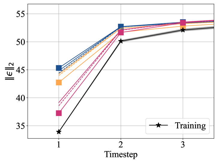
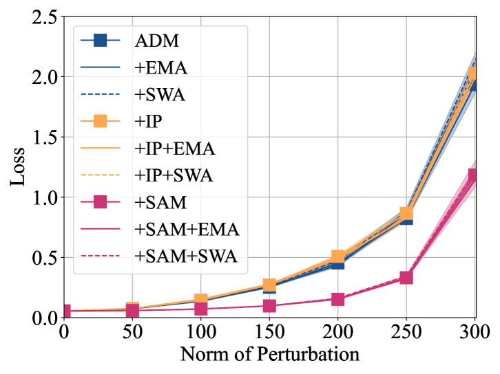
Figure 7: Additional results for CIFAR-10. We measure the L2 norm of predicted noise and loss plots under perturbation for all algorithms including +IP+EMA, +IP+SWA, +SAM+EMA, +SAM+SWA.

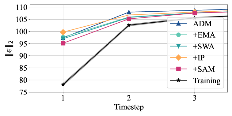
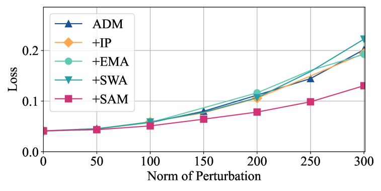
Figure 8: (Left)L2 norm of the predicted noise for LSUN Tower dataset, (Right) Loss plots under perturbation for LSUN Tower.

LPF $\downarrow$	w/o	+EMA	+SWA
ADM	0.091	0.090	0.092
+IP	0.089	0.092	0.097
+SAM	0.072	0.070	0.071

$\downarrow$: a lower value is preferred.

Table 5: Flatness measure on LSUN Tower. We calculate the loss with the perturbed model with Gaussian noise. Lower values indicate a flatter loss landscape.

In Fig. 7, we report additional results for +IP+EMA, +IP+SWA, +SAM+EMA, +SAM+SWA for CIFAR-10. We observe that ADM already possesses a certain level of flatness supporting +SWA and +EMA fail to induce additional flatness. We also report L2 norm of predicted noise loss plots under perturbation in Fig. 8 and LPF flatness in Table. 5 for LSUN Tower dataset. It coincides with the result of CIFAR-10 that +SAM induces the lower exposure bias and flatter minima.

References

- Arjovsky et al. [2017] Martin Arjovsky, Soumith Chintala, and Léon Bottou. Wasserstein generative adversarial networks. In International conference on machine learning, pages 214–223. PMLR, 2017.
- Bisla et al. [2022] Devansh Bisla, Jing Wang, and Anna Choromanska. Low-pass filtering sgd for recovering flat optima in the deep learning optimization landscape. In International Conference on Artificial Intelligence and Statistics, pages 8299–8339. PMLR, 2022.
- Blattmann et al. [2023] Andreas Blattmann, Tim Dockhorn, Sumith Kulal, Daniel Mendelevitch, Maciej Kilian, Dominik Lorenz, Yam Levi, Zion English, Vikram Voleti, Adam Letts, et al. Stable video diffusion: Scaling latent video diffusion models to large datasets. arXiv preprint arXiv:2311.15127, 2023.
- Caldarola et al. [2022] Debora Caldarola, Barbara Caputo, and Marco Ciccone. Improving generalization in federated learning by seeking flat minima. In European Conference on Computer Vision (ECCV), pages 654–672. Springer, 2022.
- Cha et al. [2021] Junbum Cha, Sanghyuk Chun, Kyungjae Lee, Han-Cheol Cho, Seunghyun Park, Yunsung Lee, and Sungrae Park. Swad: Domain generalization by seeking flat minima. Advances in Neural Information Processing Systems, 34:22405–22418, 2021.
- Chen et al. [2020] Dingfan Chen, Tribhuvanesh Orekondy, and Mario Fritz. Gs-wgan: A gradient-sanitized approach for learning differentially private generators. Advances in Neural Information Processing Systems, 33:12673–12684, 2020.
- Dhariwal and Nichol [2021] Prafulla Dhariwal and Alexander Nichol. Diffusion models beat gans on image synthesis. Advances in neural information processing systems, 34:8780–8794, 2021.
- Foret et al. [2021] Pierre Foret, Ariel Kleiner, Hossein Mobahi, and Behnam Neyshabur. Sharpness-aware minimization for efficiently improving generalization. In International Conference on Learning Representations, 2021.
- Garipov et al. [2018] Timur Garipov, Pavel Izmailov, Dmitrii Podoprikhin, Dmitry P Vetrov, and Andrew G Wilson. Loss surfaces, mode connectivity, and fast ensembling of dnns. Advances in neural information processing systems, 31, 2018.
- Granziol et al. [2020] Diego Granziol, Xingchen Wan, Samuel Albanie, and Stephen Roberts. Iterative averaging in the quest for best test error. arXiv preprint arXiv:2003.01247, 2020.
- Heusel et al. [2017] Martin Heusel, Hubert Ramsauer, Thomas Unterthiner, Bernhard Nessler, and Sepp Hochreiter. Gans trained by a two time-scale update rule converge to a local nash equilibrium. Advances in neural information processing systems, 30, 2017.
- Ho et al. [2020] Jonathan Ho, Ajay Jain, and Pieter Abbeel. Denoising diffusion probabilistic models. Advances in neural information processing systems, 33:6840–6851, 2020.
- Izmailov et al. [2018] Pavel Izmailov, Dmitrii Podoprikhin, Timur Garipov, Dmitry Vetrov, and Andrew Gordon Wilson. Averaging weights leads to wider optima and better generalization. arXiv preprint arXiv:1803.05407, 2018.
- Karras et al. [2022] Tero Karras, Miika Aittala, Timo Aila, and Samuli Laine. Elucidating the design space of diffusion-based generative models. Advances in neural information processing systems, 35:26565–26577, 2022.
- Kim et al. [2024] Kihong Kim, Haneol Lee, Jihye Park, Seyeon Kim, Kwanghee Lee, Seungryong Kim, and Jaejun Yoo. Hybrid video diffusion models with 2d triplane and 3d wavelet representation. In European Conference on Computer Vision, pages 148–165. Springer, 2024.
- Klinker [2011] Frank Klinker. Exponential moving average versus moving exponential average. Mathematische Semesterberichte, 58:97–107, 2011.
- Kwon et al. [2021] Jungmin Kwon, Jeongseop Kim, Hyunseo Park, and In Kwon Choi. Asam: Adaptive sharpness-aware minimization for scale-invariant learning of deep neural networks. In International Conference on Machine Learning, pages 5905–5914. PMLR, 2021.
- Lee et al. [2023] Hojoon Lee, Hanseul Cho, Hyunseung Kim, Daehoon Gwak, Joonkee Kim, Jaegul Choo, Se-Young Yun, and Chulhee Yun. Plastic: Improving input and label plasticity for sample efficient reinforcement learning. Advances in Neural Information Processing Systems, 36:62270–62295, 2023.
- [19] Hyun Kyu Lee and Sung Whan Yoon. Flat reward in policy parameter space implies robust reinforcement learning. In The Thirteenth International Conference on Learning Representations.
- Lee and Yoon [2024] Taehwan Lee and Sung Whan Yoon. Rethinking the flat minima searching in federated learning. In Forty-first International Conference on Machine Learning, 2024.
- Li et al. [2018] Hao Li, Zheng Xu, Gavin Taylor, Christoph Studer, and Tom Goldstein. Visualizing the loss landscape of neural nets. Advances in neural information processing systems, 31, 2018.
- Li et al. [2023a] Mingxiao Li, Tingyu Qu, Ruicong Yao, Wei Sun, and Marie-Francine Moens. Alleviating exposure bias in diffusion models through sampling with shifted time steps. arXiv preprint arXiv:2305.15583, 2023a.
- Li et al. [2023b] Puheng Li, Zhong Li, Huishuai Zhang, and Jiang Bian. On the generalization properties of diffusion models. Advances in Neural Information Processing Systems, 36:2097–2127, 2023b.
- Li et al. [2024a] Siyuan Li, Zicheng Liu, Juanxi Tian, Ge Wang, Zedong Wang, Weiyang Jin, Di Wu, Cheng Tan, Tao Lin, Yang Liu, et al. Switch ema: A free lunch for better flatness and sharpness. arXiv preprint arXiv:2402.09240, 2024a.
- Li et al. [2024b] Tao Li, Pan Zhou, Zhengbao He, Xinwen Cheng, and Xiaolin Huang. Friendly sharpness-aware minimization. In Proceedings of the IEEE/CVF Conference on Computer Vision and Pattern Recognition (CVPR), pages 5631–5640, 2024b.
- Li et al. [2023c] Xiuyu Li, Yijiang Liu, Long Lian, Huanrui Yang, Zhen Dong, Daniel Kang, Shanghang Zhang, and Kurt Keutzer. Q-diffusion: Quantizing diffusion models. In Proceedings of the IEEE/CVF International Conference on Computer Vision, pages 17535–17545, 2023c.
- Li et al. [2021] Yuhang Li, Ruihao Gong, Xu Tan, Yang Yang, Peng Hu, Qi Zhang, Fengwei Yu, Wei Wang, and Shi Gu. Brecq: Pushing the limit of post-training quantization by block reconstruction. arXiv preprint arXiv:2102.05426, 2021.
- Liu et al. [2022] Yong Liu, Siqi Mai, Minhao Cheng, Xiangning Chen, Cho-Jui Hsieh, and Yang You. Random sharpness-aware minimization. In Advances in Neural Information Processing Systems, pages 24543–24556. Curran Associates, Inc., 2022.
- Nichol and Dhariwal [2021] Alexander Quinn Nichol and Prafulla Dhariwal. Improved denoising diffusion probabilistic models. In International conference on machine learning, pages 8162–8171. PMLR, 2021.
- Ning et al. [2023a] Mang Ning, Mingxiao Li, Jianlin Su, Albert Ali Salah, and Itir Onal Ertugrul. Elucidating the exposure bias in diffusion models. arXiv preprint arXiv:2308.15321, 2023a.
- Ning et al. [2023b] Mang Ning, Mingxiao Li, Jianlin Su, Albert Ali Salah, and Itir Onal Ertugrul. Elucidating the exposure bias in diffusion models. arXiv preprint arXiv:2308.15321, 2023b.
- Ning et al. [2023c] Mang Ning, Enver Sangineto, Angelo Porrello, Simone Calderara, and Rita Cucchiara. Input perturbation reduces exposure bias in diffusion models. arXiv preprint arXiv:2301.11706, 2023c.
- Peebles and Xie [2023] William Peebles and Saining Xie. Scalable diffusion models with transformers. In Proceedings of the IEEE/CVF international conference on computer vision, pages 4195–4205, 2023.
- Qu et al. [2022] Zhe Qu, Xingyu Li, Rui Duan, Yao Liu, Bo Tang, and Zhuo Lu. Generalized federated learning via sharpness aware minimization. In International Conference on Machine Learning (ICML), pages 18250–18280. PMLR, 2022.
- Rombach et al. [2022] Robin Rombach, Andreas Blattmann, Dominik Lorenz, Patrick Esser, and Björn Ommer. High-resolution image synthesis with latent diffusion models. In Proceedings of the IEEE/CVF conference on computer vision and pattern recognition, pages 10684–10695, 2022.
- SHI et al. [2021] Guangyuan SHI, JIAXIN CHEN, Wenlong Zhang, Li-Ming Zhan, and Xiao-Ming Wu. Overcoming catastrophic forgetting in incremental few-shot learning by finding flat minima. In Advances in Neural Information Processing Systems, pages 6747–6761. Curran Associates, Inc., 2021.
- Sohl-Dickstein et al. [2015] Jascha Sohl-Dickstein, Eric Weiss, Niru Maheswaranathan, and Surya Ganguli. Deep unsupervised learning using nonequilibrium thermodynamics. In International conference on machine learning, pages 2256–2265. pmlr, 2015.
- Song and Ermon [2019] Yang Song and Stefano Ermon. Generative modeling by estimating gradients of the data distribution. Advances in neural information processing systems, 32, 2019.
- Song and Ermon [2020] Yang Song and Stefano Ermon. Improved techniques for training score-based generative models. Advances in neural information processing systems, 33:12438–12448, 2020.
- Song et al. [2020a] Yang Song, Sahaj Garg, Jiaxin Shi, and Stefano Ermon. Sliced score matching: A scalable approach to density and score estimation. In Uncertainty in artificial intelligence, pages 574–584. PMLR, 2020a.
- Song et al. [2020b] Yang Song, Jascha Sohl-Dickstein, Diederik P Kingma, Abhishek Kumar, Stefano Ermon, and Ben Poole. Score-based generative modeling through stochastic differential equations. arXiv preprint arXiv:2011.13456, 2020b.
- Song et al. [2023] Yang Song, Prafulla Dhariwal, Mark Chen, and Ilya Sutskever. Consistency models. 2023.
- Wang et al. [2023] Zhendong Wang, Yifan Jiang, Huangjie Zheng, Peihao Wang, Pengcheng He, Zhangyang Wang, Weizhu Chen, Mingyuan Zhou, et al. Patch diffusion: Faster and more data-efficient training of diffusion models. Advances in neural information processing systems, 36:72137–72154, 2023.
- Wu et al. [2025] Junyi Wu, Haoxuan Wang, Yuzhang Shang, Mubarak Shah, and Yan Yan. Ptq4dit: Post-training quantization for diffusion transformers. Advances in Neural Information Processing Systems, 37:62732–62755, 2025.
- [45] Tianshuo Xu, Peng Mi, Ruilin Wang, and Yingcong Chen. Why diffusion models are stable and how to make them faster: An empirical investigation and optimization.