Self-calibration in two dimensional aperture mask optical interferometry: a new method for wavefront sensing

Abstract

We present a new methodology in optical aperture masking interferometry involving Fourier analysis of the complex visibilities (real and imaginary, or amplitude and phase), derived from the interferometric images. The analysis includes use of a non-redundant aperture mask, and self-calibration of the hole-based complex voltage gains to correct for non-uniform illumination and phase fluctuations across the mask. The technique is demonstrated using the Synchrotron Radiation Interferometry (SRI) facility at the ALBA synchrotron light source. Application of the technique results in a joint derivation of the Gaussian shape of the electron beam, and of the hole-based voltage gain amplitude and phase distribution over the mask area. The gain phases are linearly related to the photon path-lengths through the optical system for the ray to each hole, and hence represent an accurate wavefront sensor (WFS) determining the path-length distortions across the wavefront. Wavefront sensing is a vital technology in fields ranging from adaptive optics to metrology to optometry. We calculate that the rms precision of this WFS method is better than 1 nm per frame in the current experiment. We compare the technique to the standard Shack-Hartman WFS. We also show that a structure-agnostic imaging and deconvolution process can be used with the visibility data to determine the beam shape without assuming a Gaussian model, and hence the technique is generalizable to more complex source morphologies.

1 Introduction

Aperture masking interferometry of optical synchrotron radiation is commonly used in monitoring the relativistic electron beam size and shape at synchrotron light sources [1, 2]. The most common practice of synchrotron radiation interferometry (SRI) at accelerators involves simple two-slit interferometry with Gaussian model fitting to the measured sinusoidal fringe amplitudes (coherences), and slit rotation to obtain the 2-dimensional (2-D) measurement. Recently, we introduced a technique using a 2-D aperture mask involving Fourier analysis of the measured coherences, or visibilities, in the u,v-plane, incorporating a non-redundantly sampled mask to avoid decoherence of redundant samples [3], and self-calibration of the voltage amplitudes at each hole to correct for non-uniform illumination across the mask [4, 5].

In this report, we expand the Fourier analysis to include self-calibration of the full complex visibilities (real and imaginary or amplitude and phase), which provides both a measurement of the source size and shape, as well as the element-based voltage gain amplitude and phase corrections, where an interferometric element corresponds to a hole in the mask. The element-based gain phases provide a measure of the relative photon path-lengths through the optical system to the aperture plane, and hence represent an accurate wavefront sensor for the distortions across the wavefront.

In our previous analysis, we relied on the fact that the electron beam shape is known to be Gaussian in order to limit the self-calibration and model fitting to just the amplitudes of the visibilities, and hence to derive both source size and hole gain amplitudes. We also employed a second method for beam size determination from the visibility data which relies on quantities known as ‘closure amplitudes’. Closure amplitude is a combination of visibilities which is invariant to variations in the illumination pattern [6]. This method also relies on the fundamental assumption of a Gaussian shaped source, and results in a beam size determination consistent to within a few percent of other methods [7].

Our expanded self-calibration analysis now includes the visibility phases in the generalized complex voltage gain solutions. Including both phase and amplitude gain solutions allows for a more general approach to the Fourier imaging, self-calibration, and deconvolution process. Such a more general analysis has been applied to sources of complex morphological shape in radio astronomy [8, 9, 10, 11]. We also demonstrate that the Gaussian shape of the source can be recovered from the self-calibrated visibilities through a structure-agnostic Fourier imaging and deconvolution process.

In Section 6 we present the process of wavefront sensing using the element-based phases from the self-calibration process. We discuss the potential advantages, disadvantages, precision, and dynamic range of this process compared to the standard Shack-Hartmann wavefront sensor.

2 Basic Concepts

3 Basics of Interferometric (Fourier) Imaging and Self-Calibration

The spatial coherence (or visibility), $V_{ab}(\nu)$, corresponds to the cross correlation of two quasi-monochromatic voltages of frequency $\nu$ of the same polarization measured by two spatially distinct elements in the aperture plane of an interferometer. The visibility relates to the intensity distribution of an incoherent source in the far field, $I(\hat{\mathbf{s}},\nu)$, via the van Cittert-Zernike theorem [12, 13], which after certain approximations reduces to a Fourier transform [6, 14]:

$$V_{ab}(\nu) =\int_{\textrm{source}}A_{ab}(\hat{\mathbf{s}},\nu)I(\hat{\mathbf{s}},\nu)e^{-i2\pi\mathbf{u}_{ab}\cdot\hat{\mathbf{s}}}\mathrm{d}\Omega\,,$$ (1)

where, $a$ and $b$ denote a pair of array elements (eg. holes in a mask), $\hat{\boldsymbol{s}}$ denotes a unit vector in the direction of any location in the image, $A_{ab}(\hat{\mathbf{s}},\nu)$ is the spatial response (the ‘power pattern’) of each element (in the case of circular holes in the mask, the power pattern is the Airy disk), $\mathbf{u}_{ab}=\mathbf{x}_{ab}(\nu/c)$ is referred to as the “baseline” vector which is the vector spacing ($\mathbf{x}_{ab}$) between the element pair expressed in units of wavelength, and $\mathrm{d}\Omega$ is the differential solid angle element on the image (focal) plane. In practice, a visibility is charactrized by a ’spatial fringe’ of sinusoidal spatial frequency and orientation determined by the baseline vector, and has an amplitude, corresponding to the power of the source mutual coherence at that fringe spacing, and a phase corresponding to the position of that fringe relative to the adopted phase center.

In radio interferometry, the voltages at each element are measured by phase coherent receivers and amplifiers, and visibilities are generated through subsequent cross-correlation of these voltages using digital multipliers [6]. In the case of optical aperture masking, interferometry is performed by focusing the light that passes through the mask (the aperture plane element array), using reimaging optics (effectively putting the mask in the far-field, or Fraunhofer diffraction), and generating an interferogram on a CCD detector at the focus. The visibilities can then be generated via a Fourier transform of the interferogram or by sinusoidal fitting in the image plane.

However, the measurements can be corrupted by distortions introduced by the propagation medium, or the relative illumination of the holes, or other effects in the optics, that can be described, in many instances, as a multiplicative element-based complex voltage gain factor, $G_{a}(\nu)$. Thus, the corrupted measurements are given by:

$$V_{ab}^{\prime}(\nu) =G_{a}(\nu)\,V_{ab}(\nu)\,G_{b}^{\star}(\nu)\,,$$ (2)

where, $\star$ denotes a complex conjugation.

The process of interferometric self-calibration determines these complex voltage gain factors in parallel with determining source structure. A physically reasonable starting model for the source is assumed, $V_{ab}(\nu)$. Using the measurements, $V_{ab}^{\prime}(\nu)$, Equation (2) is then inverted to derive the complex voltage gains, $G_{a}(\nu)$, using an optimization criterion, such as least squares fitting [15, 11, 10, 16]. A new source model is then derived from the gain-corrected visibilities through model fitting or imaging (Fourier inversion) and deconvolution, and the process is iterated until convergence. The process converges since there are typically more measurements ($[N(N-1)]/2$ complex cross correlations, or visibilities, where $N$ is the number of interferometric elements), than fitted parameters ($N$ element-based complex gains, and model parameters), at least for reasonably sampled visibility data and a not-too-complex source [15, 11]. In our experiment, for a single 7-hole mask image, there are 43 measurements (the real and imaginary parts, or amplitude and phase, from each of the 21 complex-valued visibilities, plus one positive-valued autocorrelation). And there are 17 unknowns: the Gaussian source flux, major and minor axes, and major axis position angle, and the voltage gain amplitude and phase for each element.

In the case of SRI at ALBA, we have previously employed self-calibration assuming a Gaussian shape for the synchrotron source, the details of which are presented in [4]. In [4], the source shape recovery and self-calibration process considered only the gain voltage amplitudes, corresponding to the square root of the flux through an aperture (recall, power $\rm\propto voltage^{2}$), dictated by the illumination pattern across the mask. Coupled with the assumption of a Gaussian shape for the source (well documented via eg. X-ray pinhole measurements [17]), both the element-based voltage amplitudes and source shape parameters can be derived with this process, without use of the visibility phases.

In this report, we perform a generalized complex self-calibration process, starting from a point source model. In particular, we now include both element-based voltage phase and amplitude self-calibration. Such a generalized process, while not absolutely necessary in this case where the source is known to be of Gaussian shape, will allow for future imaging of more complex sources. And again, the gain phases represent a new type of wavefront sensing, which we discuss in Section 6.

4 Rotated mask data and CASA self-calibration

4.1 Data processing

All measurements were made at the optical SRI lab at the ALBA synchrotron light source. The details of the optical system are presented in the recent papers by [4, 5]. Figure 1 shows a simplified schematic of the SRI system optics, without showing the full optical path, which includes 8 flat mirrors before the mask, including the cooled pickoff mirror closest to the source (1.64 m, [17]). Figure 1 also shows a cartoon of the corrugation of the wavefront that may occur during propagation through the optical system (see Section 6).

In our new analysis we employ a 7-hole non-redundant mask with 2 mm diameter holes. The mask geometry is a stretched and scaled version of the aperture mask employed at the James Web Space Telescope [18]. The JWST mask was optimized for imaging of exoplanetary systems. A schematic of the mask is shown in Figure 2.

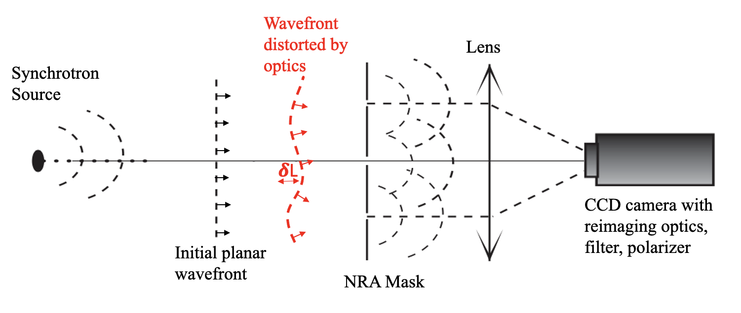
Figure 1: Idealized optical SRI system without showing all the mirrors (total of 8 flat mirrors from the source to the mask). A cartoon of the wavefront distorted by the optics and/or laboratory turbulence is shown.

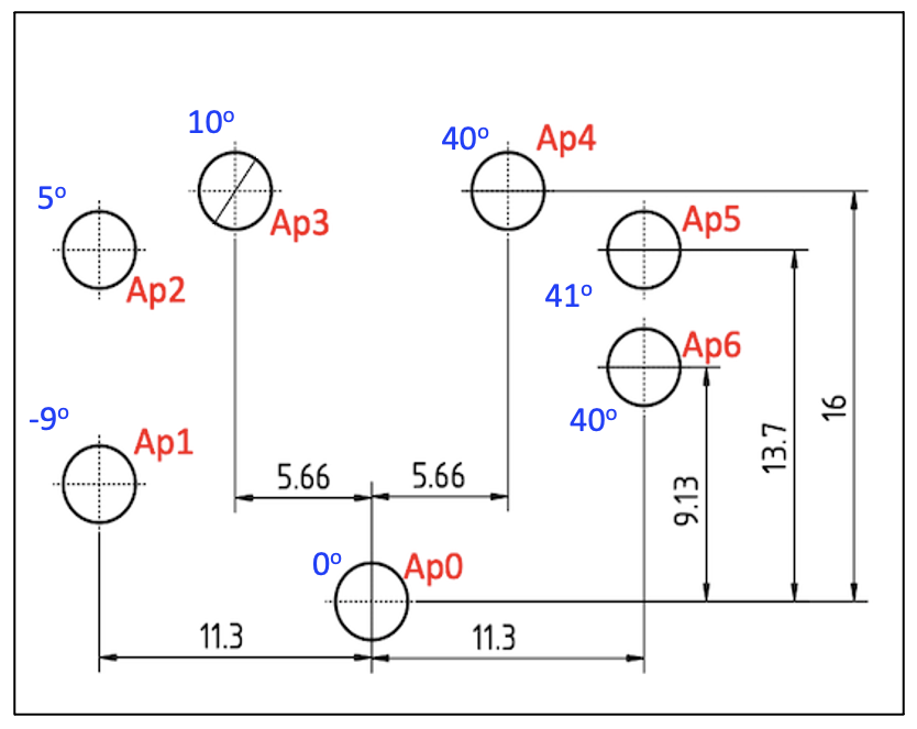
Figure 2: Scale drawing of the 7 hole mask with the hole numbers listed in red. Hole phase gains for one frame in the time series are shown, after subtracting the mean gain phase for the time series.

A CCD camera was employed to obtain images of the diffraction pattern with a narrow band filter at 400 nm. Each frame exposure was 0.3 ms in duration, and 30 frames were taken with a frame separation of 1 s for each experiment. In the following analysis, we employ four mask rotation angles to increase the coverage of the aperture plane: 0^∘, 27^∘, 335^∘, 341^∘.

Figure 3 shows the Fourier spacing, or $u,v$ coverage, for the interferometric baselines defined by the mask hole distribution. The coverage for all four rotation angles is shown, as well as the coverage for just the 0^∘ mask.

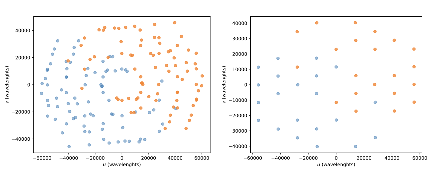
Figure 3: Left: $u,v$ coverage for the 400 nm data for all four mask rotation angle images. Right: same but for only the 0^∘ rotation image.

We employ the same Fourier processing steps to go from CCD images to visibilities as in [4]. For reference, a CCD bias of 3.25 was used, and images were padded to 2048 pixels prior to Fourier transforming. Each padded image frame was centered on the mean Airy disk peak from all 30 frames in a given experiment, before Fourier transforming. The visibilities were derived from the complex Fourier transform product images by locating the positions of each visibility and using aperture photometry with a radius of four $u,v$ pixels.

Note that we perform our analysis in angular coordinates. For reference, given the geometry of the optical system, in the image plane the FWHM of the Airy disk for a 2mm hole is given by: $\textrm{FWHM}=1.03\times\lambda/D~\textrm{rad}=41^{\prime\prime}$, where $\lambda$ is the wavelength and $D$ is the diameter of the aperture. The fringe spacing (peak to peak) for an interferometric baseline, $B$, is $\lambda/B$ rad. For a 22mm baseline in the mask, the fringe spacing is then $3.7^{\prime\prime}$. For comparison, the FWHM of the electron beam synchroton source at ALBA is $1.9^{\prime\prime}\times 0.70^{\prime\prime}$ (140 $\mu$m $\times$ 56 $\mu$m at 15 m distance). While the source is smaller than the fringe spacing, the very high signal-to-noise of the measurements (millions of photons per frame), allows for very accurate model fitting to obtain information on source structure smaller than the fringe spacing [19].

4.2 CASA self-calibration

The visibilities were then loaded into a CASA measurement set format for analysis using the CASA software. An empty measurement set was generated using the SIMOBSERVE task, preserving the $u,v$ plane angular geometry as well as the primary beam (Airy disk) size. A PYTHON routine was written to then fill the empty visibilities with the SRI measurements. CASA has a well developed software suite of interferometric calibration, model fitting, and imaging with deconvolution long used in radio astronomy, but equally applicable in the current context [20].

Figure 4 shows the Fourier transform of the $u,v$ coverage for all four mask rotation angles, then the same but for just the 0^∘ rotation angle These images represent the point spread function (PSF) in the image plane of the $u,v$ coverage, meaning the convolution function for the imaging response of the interferometric mask. The $u,v$ coverage for a single mask image shows a regular spacing between columns in the horizontal direction, and a less pronounced, but still extant, grid-spacing in the vertical directions. This grid-like spacing leads to grating lobes (secondary peaks also referred to as sidelobes), as seen in the PSF. Including all 4 rotations decreases these grating lobes substantially (30% vs. 71%), which is the primary impact of the improved $u,v$ coverage with rotation (84 visibilities vs. 21). Note that for a simple, small source, such as is the case herein, the grating lobes will not have a major impact on image quality after deconvolution, because there are no issues with ’confusing’ sources across the field, as is often the case in astronomical applications.

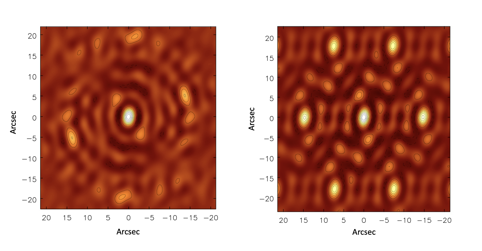
Figure 4: Left: Point spread function with all 4 rotation angle $u,v$ data. Contour levels start at 10% and increase in increments of 10%. Right: Point spread function for the 0^∘ frame.

As a check on the validity of the self-calibration process in CASA, we have analyzed one frame from each of the 7-hole rotated mask dataset, performing self-calibration in two ways. First is the amplitude-only self-calibration assuming a Gaussian model via GAUSSFIT routine as used in [4]. The second method is full complex self-calibration (real and imaginary, or amplitude and phase), in CASA using the best Gaussian model from the [4] analysis for the gain calibration, and then using UVMODELFIT in CASA to fit a Gaussian to the self-calibrated data. All of the results agree to within 5% in the derived major and minor axis dispersions for the source, and within $3^{\circ}$ for the major axis position angle. We also compare the derived hole-based amplitude voltage gains as derived in CASA, with those from the amplitude-only process in [4] , and find agreement typically within 1%.

5 CASA self-calibration starting from a point source model

5.1 Self-calibration and model fitting

The standard astronomical self-calibration procedure involves starting the process with visibility self-calibration using a very simple model, such as a point source. A new source model is then derived from the self-calibrated data either through model fitting or some form of PSF deconvolution, and a second iteration of self-calibration is then performed using the new model. The process then continues until the model and gain solutions no longer change substantially between iterations.

In our case, each calibration step of the self-calibration cycle must be done on data from rotated masks exposures separately, since the gain phases vary between exposures due to vibration of the optics and/or laboratory turbulence. However, the updated model in each step can be obtained by joint fitting to all the self-calibrated data. Hence, the self-calibration has 21 visibilities per rotation, but the model fitting has 84 visibilities.

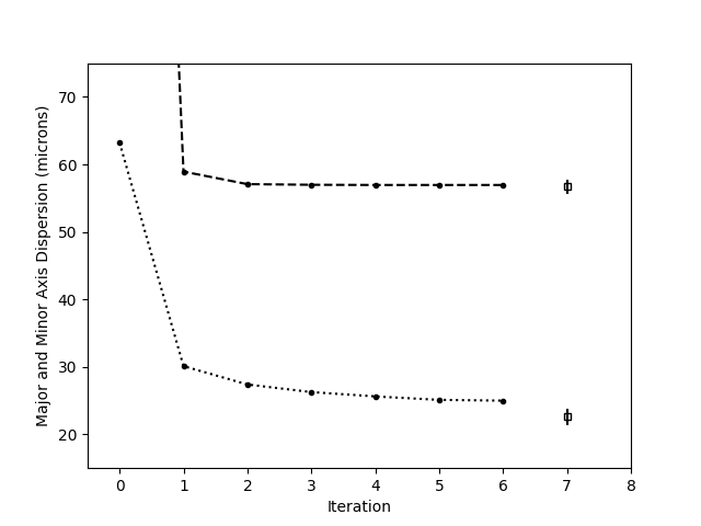
Figure 5: Derived major and minor axis dispersions for each iteration of self-calibration in CASA. The zero iteration point is with no self-calibration, and the fitting results are poor since there is little phase coherence. The first iteration (phase-only point source self-cal), already guides the process toward the correct answer. The point at iteration 7 shows the mean value derived from the amplitude only self-cal process in [4], applied to each rotation angle data set individually. The error bars indicate the peak to peak scatter in the four measurements.

As a demonstration, we employ one data frame from each mask rotation, and start the self-calibration process with a point-source model and perform phase-only self-calibration, to improve coherence. The subsequent model is derived by Gaussian fitting using the CASA routine UVMODELFIT. The resulting Gaussian parameters are used to generate a new model for self-calibration, and the process is iterated.

Figure 5 shows the results from the self-calibration process as a function of iteration. The 0 iteration corresponds to the raw data (no self-cal). In this case, the fitted Gaussian parameters are nonsensical, due to the lack of visibility coherence (semi-random phases), ie. the fitted major axis is almost a factor 5 larger than the expected value. However, iteration 1, corresponding to a single phase-only self-calibration with a point source model, lines up the visibility phases, thereby restoring coherence in the image plane, and improves the fitting dramatically, with the axes within 20% of the expected value.

Subsequent iterations involve phase and amplitude self-calibration, to correct for both the phase screen and non-uniform illumination across the mask. The process converges quickly. The open symbols at iteration 7 show the mean values of the parameters derived from the amplitude-only self-calibration and Gaussian fitting process in [4]. The major and minor axes derived in the CASA processing converge to within 2$\mu$m of the size expected, or better than 10%. The major axis position angle converges to 19.0^∘ in CASA, within $1^{o}$ of the expected value, where the expected values are based on both the amplitude-only self-calibration process, as well as independent methods, such as the X-ray pinhole [17].

5.2 Deconvolution

As opposed to Gaussian model fitting to the visibilities to obtain source parameters, an alternative, potentially more general, method of recovering source morpohology is by using a deconvolution process, in which the image convolution kernel (the point spread function of the interferometer), is deconvolved from the image, making physically reasonable assumptions about the expected true source brightness distribution. One standard method for deconvolution is the CLEAN algorithm, in which the source is assumed to be comprised of delta functions, and their locations and brightnesses are iteratively found in the ’dirty’ image (ie. the image convolved with the PSF), and subtracted from the $u,v$ data [21, 22]. CLEAN can be considered a ’model fitting’ approach, in which the model is comprised of point sources [23].

We have performed such a CLEAN deconvolution of the ALBA visibility data using the task IMAGR in the Astronomical Image Processing Software (AIPS). For Fourier imaging and deconvolution, we used an image cell size of 0.1$"$, an image size of 1024, and 500 CLEAN iterations with a CLEAN loop gain of 0.02. The Gaussian fitted beam to the PSF for the 400 nm data has: $\rm FWHM=3.40"\times 2.10"$, with a major axis position angle of $-8.1^{\circ}$ (Figure 4). Again, the measurement has very high signal-to-noise, so we restore the CLEAN components with a Gaussian convolution kernel of $\rm B_{maj}=B_{min}=1.5"$, meaning a modest ’hyper-resolution’.

The resulting image is shown in Figure 6, along with the surface brightness profile along the major axis. A Gaussian fit to the CLEAN image (not to the $u,v$ data as previously), results in a deconvolved source size of $1.79"\times 0.28"$, PA = $16.8^{\circ}$. The expected major axis size and the position angle are reproduced in the deconvolved image to within a few percent, but the minor axis is poorly determined. The poor fit to the minor axis reflects the limits of such a deconvolution process with hyper-resolution in the case of sparse $u,v$ coverage.

The fact that we can reproduce the expected Gaussian source, at least in the major axis and position angle, with limited $u,v$ coverage, using CLEAN deconvolution (which is a relatively source-structure agnostic deconvolution process), lends confidence that more complex sources, such as is the case for free electron lasers [24, 25], can be recovered using interferometric masks with more complete $u,v$ coverage, through an iterative deconvolution and self-calibration process. This iterative reconstruction technique has been abundantly demonstrated in radio astronomical interferometric imaging of very complex celestial sources [23].

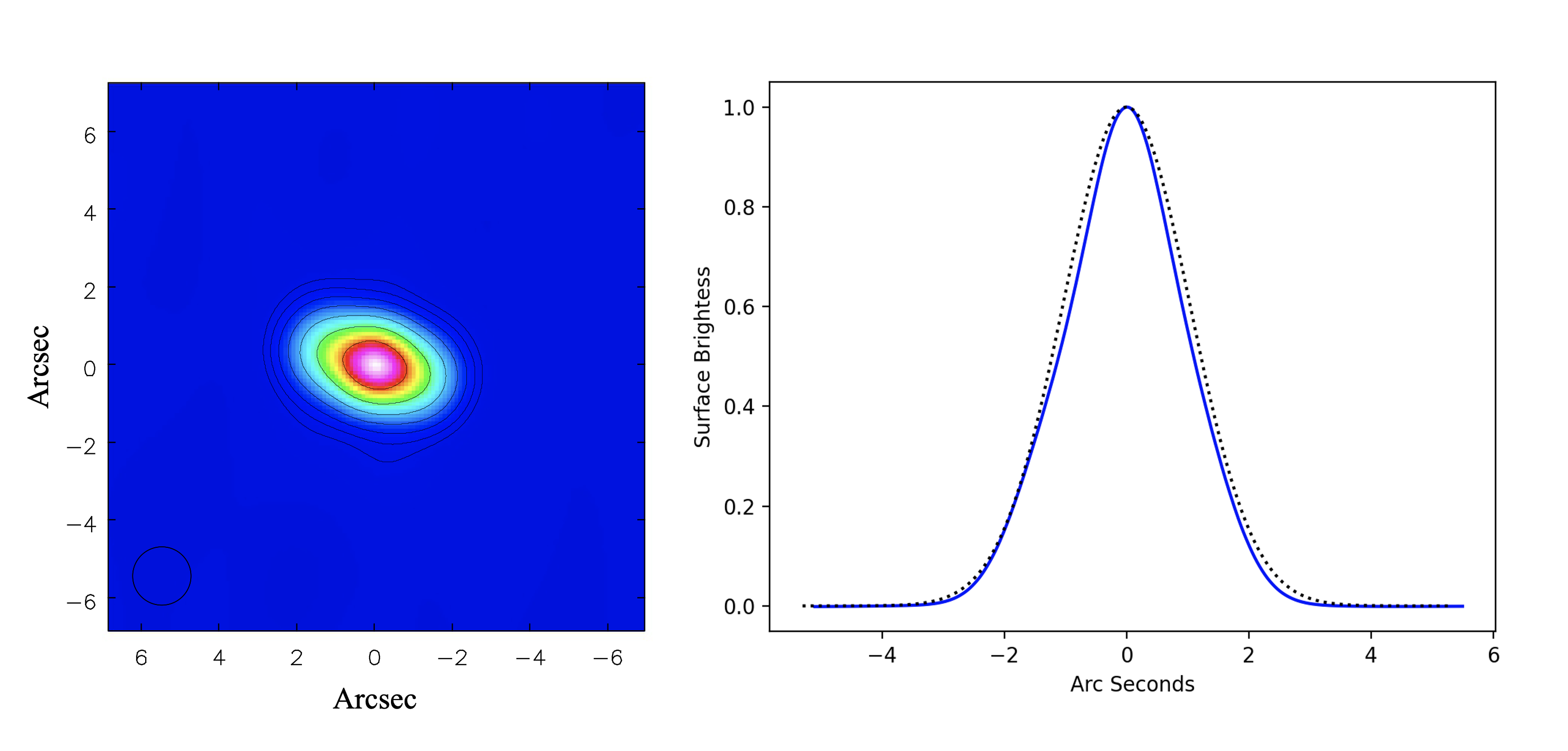
Figure 6: Left: CLEAN deconvolved image from IMAGR in AIPS of the self-calibrated 400nm data. The CLEAN delta function components have been convolved with a circular Gaussian of $\rm FWHM=1.5"$. The contour levels are a geometric progression in factors of 2, starting at 1%. Right: The surface brightness profile along the major axis. The blue line is the image, and the dotted line is the expected source size, also convolved with a $1.5"$ Gaussian.

6 Wavefront Sensing

6.1 General Concepts

An electromagnetic wavefront is defined as the plane perpendicular to the direction of propagation of the EM wave, corresponding to the plane of equal phase. Wavefront distortions due to non-ideal optical components, or due to turbulence in the laboratory atmosphere, can lead to ’corrugations’ in an initially planar wavefront, corresponding to path-length delays across the wavefront as it transverses the optical system (see Figure 1). Wavefront sensing corresponds to methods designed to determine these path-length delays [26].

Wavefront sensing has a wide range of uses, including: (i) real-time adaptive optics to correct for turbulence or vibrations of optical components in astronomical and laboratory systems [27], (ii) surface metrology of physical components to high accuracy [28], and (iii) even in medical optometry to determine the shape of the cornea in order to then apply corrective methods, such as Lasik surgery [29, 30, 31].

The principle methods of wavefront sensing in use today fall into two categories [32]: (i) reference wave interference methods, and (ii) angle-based wavefront sensors. The reference wave technique is based on Fizeau-interferometry, where beam splitting is used to interfere the target wavefront with a ’reference wavefront’, either a copy of the original wavefront reflected off a known reference surface, or an independently generated reference wavefront. This method requires a well calibrated and stable reference surface, or second light source, in order to determine the target wavefront distortions. Recent application of a Talbot WFS at the LCLS can be classified into the reference wave method, where the ‘Talbot images can be treated as interferograms formed by sheared copies of the original wavefront’ [33].

The most common form of angle-based wavefront sensor is the widely used and developed Shack-Hartmann wavefront sensor [34], and variations thereof. The SHWFS involves a lenslet aperture array which images a planar incoming wavefront into a uniform grid of sources in the focal plane. Wavefront corrugations then distort this grid due to the different angle of incidence at each lenslet. The local offsets of a source from the expected grid point determines the phase gradient of the incident plane wave across that particular lenslet. SHWFS therefor measures the wavefront gradient distribution across the wavefront (first derivative). Fitting of smooth functions to the gradient distribution, such as 2D Zernike polynomials, is then used to determined the dominant modes for path-length distortions of the wavefront across the aperture [35]. SHWFS have been developed with few nanometer accuracy and with dynamic ranges in the hundreds, or even a thousand, where dynamic range corresponds to the largest optical path-length distortion measurable, in units of wavelengths.

The self-calibration phase solutions in our processing represent a new approach to wavefront sensing, in which the gain phases, $\phi_{G}$, are linearly proportional to wavefront path-length delays across the mask, $\rm\delta L(t)$, relative to the reference hole, through the simple relation:

$$\rm\delta L=\lambda\times(\phi_{G}/360^{\circ}),$$ (3)

where $\rm\phi_{G}$ is in degrees. Hence, the gain phases correspond to an accurate (small fraction of a wavelength), high time resolution wavefront sensor. We discuss phase wraps in Section 7.2.

In the following sections, we consider the gain phase solutions from our self-calibration process in the context of potential application to wavefront sensing. We also analyze visibility phases as a demonstration of the spatial correlations indicative of wavefront distortions across the aperture. We consider both short timescale phase distortions, relevant for adaptive optics systems, and slow or static wavefront distortions, more relevant for metrology or optometry. In Section 7.2 we consider limitations to the process, including precision and dynamic range.

6.2 Rapid Variations: Phase jitter (seconds)

In this section, we investigate the visibility phases both before and after calibration on one second timescales from the 30 frames in a given experiment, using the best Gaussian model for the 7 hole data. We then consider the hole-based gain phase variations on the same timescale.

Note that our exposure time per frame is 0.3 ms, but the frame rate is one per second, so we have no direct information on the phase variation on timescales shorter than one second. However, we have performed tests with longer frame exposure times (1 ms or greater), and find that the visibility amplitudes decrease with increasing exposure time, suggesting decoherence due to phase jitter on timescales of order 1 ms [36].

Figure 7 shows the visibility phase time series for all baselines to hole 5 before calibration. Phase variations with an rms scatter of tens of degrees are evident. Two trends are clear: first, spatially close baselines (eg. 1-5 and 2-5), show correlated phase structure in their time series. Second, the longer baselines show larger phase fluctuations than the shorter baselines. Figure 7 also shows the rms of the phase time series for all baselines vs. baseline length. A powerlaw fit results in a close to linear increase in rms phase fluctuations with baseline length, with index of $0.87\pm 0.14$.

The path-length delay, or phase jitter, at ALBA is thought to be dominated by vibration of the optics, with a possible contribution from turbulence in the laboratory atmosphere. A linear increase of visibility phase rms with baseline length (Figure 7), and a correlation between close baselines (see also Figure 8), would be expected if the dominant vibration term is tip-tilt, corresponding to the lowest spatial mode.

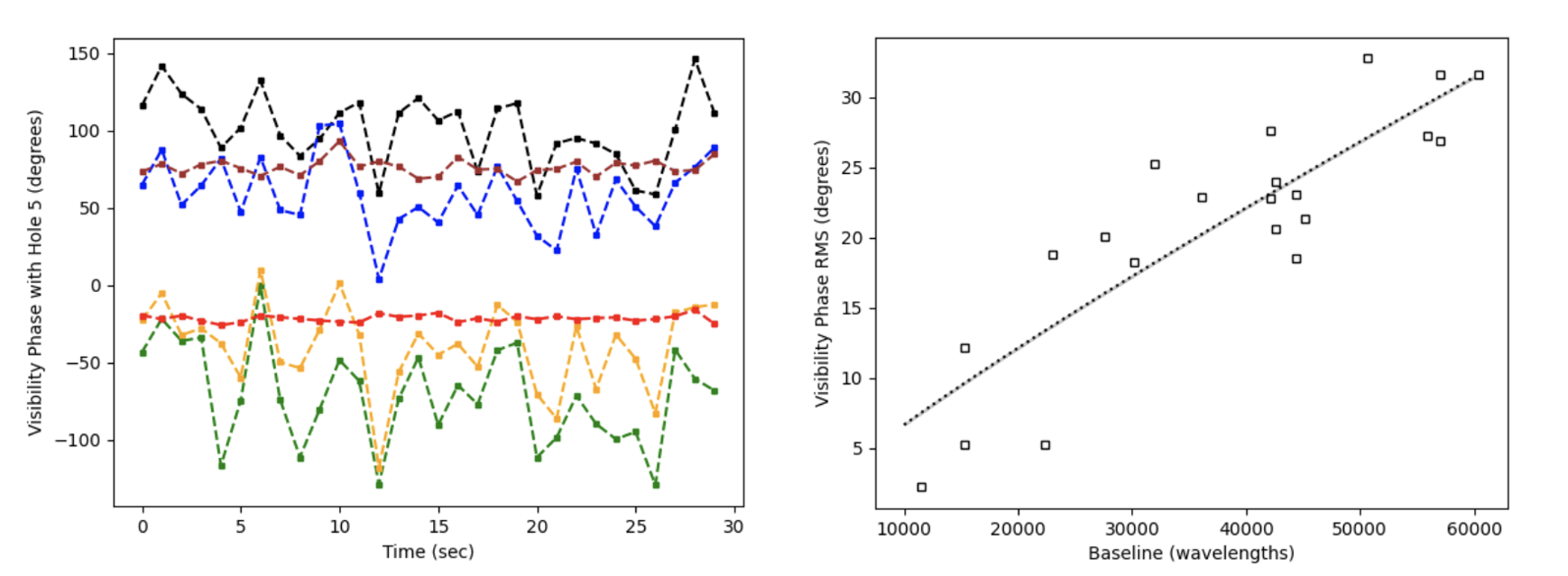
Figure 7: Left: visibility phase time series for all baselines to hole 5. Black = 0-5; Green = 1-5; Orange = 2-5; Blue = 3-5; Brown = 4-5; Red = 5-6. Right: The rms of the visibility phase time series vs. baseline length, in wavelengths. The dotted line is a powerlaw fit with an index of $0.87\pm 0.14$.

Figure 8 shows a comparison of the visibility phases on two close, parallel baselines, namely 1-6 and 2-5, both before and after calibration. In this case, the baselines do not share a hole, as was the case in Figure 7. Before calibration, the phase fluctuations of the time series are large (rms values $\sim 30^{\circ}$), and closely correlated between the two baselines, even though, in this case, the baselines do not share a hole.

After calibration, the rms variations in Figure 8 over the 30 time samples are $\sim 1.2^{\circ}$, and there is no residual correlation between baselines. Recall there are of order $10^{6}$ photon counts per visibility in our analysis, so the root(N) noise due to photon counting statistics should be of order 0.1%, which, in phase implies $\sim 0.4^{\circ}$, or a factor three lower than our empirical rms measurement. There are other steps in the processing that might add a random noise-like term other than the minimum set by photon counting statistics, as summarized in [4]. One possible contribution comes from the pixelization of the image: the phase of a visibility is the shift of the fringe pattern on the CCD relative to the reference pixel, and the accuracy with which this can be measured is determined by the pixel size and signal to noise. We note that the rms fluctuations of the closure phase time series for the ALBA SRI experiment are also around $\sim 1^{o}$ [36]. Closure phase is a quantity that is invariant to hole-based complex gain phases, hence lending credence to the post-calibration rms phase fluctuations in Figure 8 representing a noise-like (uncorrelated) limit to the visibility phase measurements.

The analysis of Figure 8 has two important implications. First, the fact that before calibration the visibility phase fluctuations correlate between close, parallel baselines that do not share a hole implies that the pre-calibration phase jitter is not due to a random noise term, such as photon counting statistics, but reflects some systematics of propagation that has spatial correlation, such as vibration of optical components or lab turbulence. And second, the fact that the noise-like post-calibration phase jitter is a factor 30 lower than pre-calibration phase jitter, implies that the vibrational or turbulence induced phase jitter is being measured at high signal-to-noise. We return to this point in Section 7.2 below.

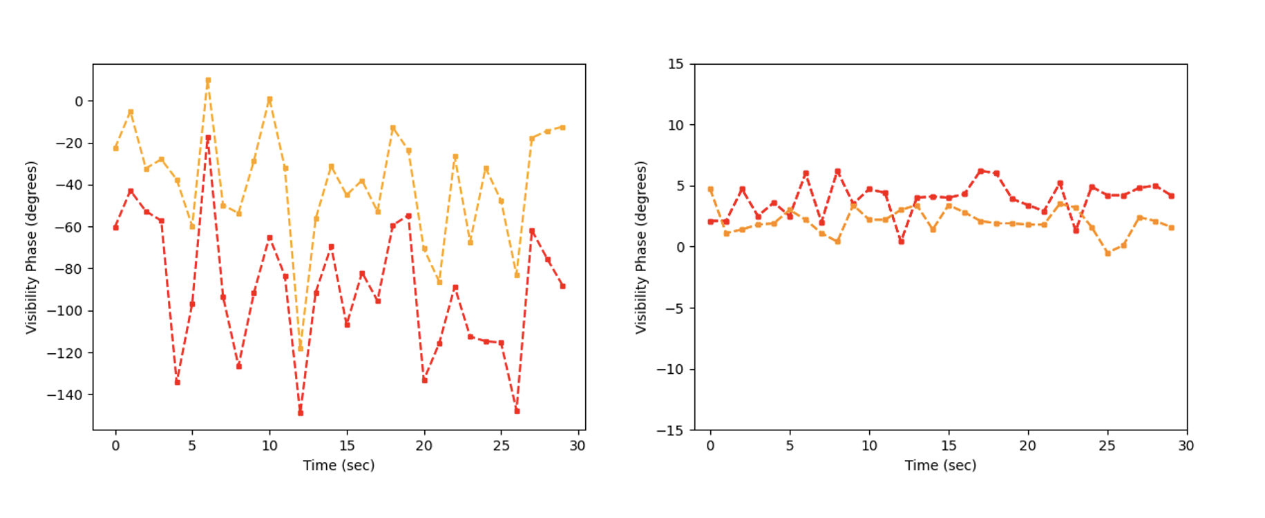
Figure 8: Visibility phase time series of baseline 1-6 (red) and 2-5 (orange). These are two close and parallel baselines that do not share a hole. Left: before calibration. Right: after calibration. The phase fluctuations are clearly correlated between baselines before calibration even though these baselines do not share a hole, implying some coherence of the phase screen across the mask, and not random phase noise. After calibration, there is no correlation of the residual phase jitter between baselines. Note the Y-axis range is much larger for the left-hand figure.

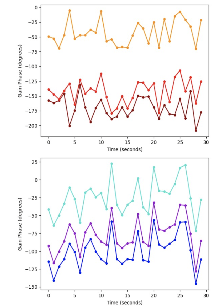
Figure 9: Gain phase solutions vs. time for the 6 holes. Holes on the left side of the mask are shown in the upper plot (1=dark red, 2=red, 3=orange), and the lower plot shows the three holes on the right side of the mask (4=turquoise, blue=5, violet=6; hole 0 is the phase reference hole with gain phase of $0^{\circ}$ by construction).

Turning to phase gains from self-calibration, Figure 9 shows the gain phase solution for the 30 second time series for the holes. The plots are separated into the three holes on the left side of the mask (1,2,3), and the three on the right of the mask (4,5,6) (Figure 2). The gain phase solutions correlate between closer holes, with little or no correlation seen for large hole separations. A cross-correlation analysis of the time series shows that gain phases for close separation holes (such as 1 and 2, or 5 and 6), are well correlated at $>5\sigma$ for the zero-lag point, while more widely separated holes (like 1 and 6), show no clear correlation in phase gains ($<2\sigma$ at zero lag, where $\sigma$ is derived as the rms scatter of the non-zero lag points).

Referring back to Figure 2, the phase gains for each hole in one exposure are shown, after subtracting the mean phase from the full time series. These residual gain phases per frame are measured also after mean Airy disk centering of the frame prior to Fourier transfer (Section 4.1). Hence, these residuals represent the jitter of the wavefront after removing the static terms (mean centering and mean gain phase).

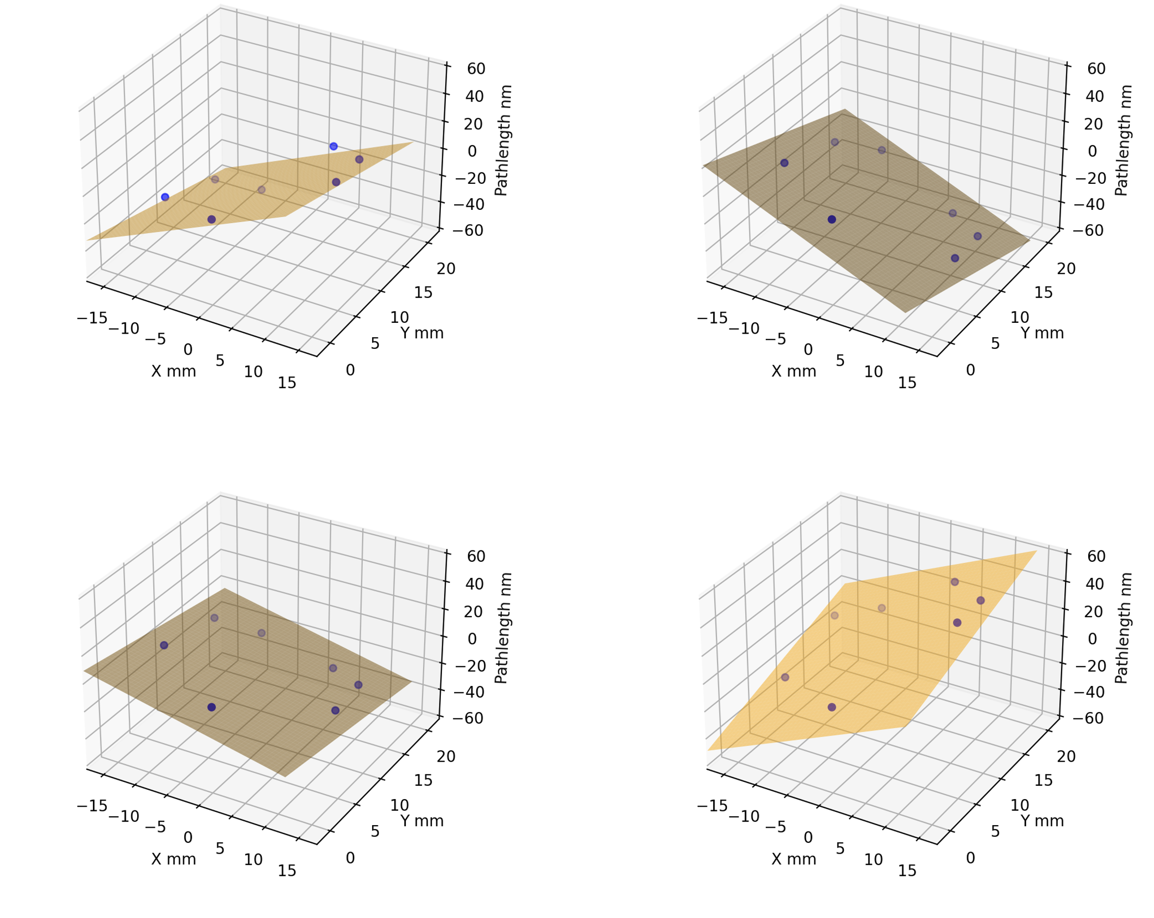
Figure 10: Three-dimensional projections of the residual path-length variations for four frames from the 7-hole mask, after mean Airy disk centering and subtracting the mean gain phase for the full time series, and converted to pathlength in nanometers using Equation 3. These residual path-lengths represent the jitter of the wavefront after removing the static terms. Also shown is a best-fit planar wavefront to the points, corresponding to the dominant tip-tilt term for the wavefront.

We can convert these residual gain phases to path-length using Equation 3. Figure 10 shows the result of a planar tip-tilt fit to the residual path-lengths for the 7-hole mask for four frames in the time series. The planar fits show a peak-to-peak tilt of $\leq\pm 50$ nm across the mask. The plane orientation varies randomly between frames taken every one second, as expected since the jitter occurs on millisecond timescales, as implied by analysis of the visibility coherence with exposure time [36].

The points scatter above and below the plane by typically a few to 10 nm. This scatter corresponds to higher order corrugation modes in the wavefront due to flexing of the optical components, and/or laboratory turbulent structure across the wavefront, with a contribution from random noise (see Section 7.2). Aperture masks with better sampling (more holes) will allow for fitting of the higher order modes.

6.3 Slow and Static Variations (hourly): Mirror Temperature Tests

The existence of static, or very slowly varying, path-length differences across the field can be seen even in the visibility phases. Figure 7 shows that, before calibration, the distribution of the mean phases for the different baselines covers a wide range ($\sim-75^{\circ}$ to $+100^{\circ}$), while after calibration, the mean phases converge to zero phase, as expected for a Gaussian source at the field center (Figure 8). The pre-calibration mean visibility phases represent roughly static path-length differences through the optical system.

We next consider long timescale (hourly) changes in the phase gain solutions, as other aspects of the system slowly change. We perform a test where measurements are made every hour for 24 hours, starting with the insertion of the optical pick-off mirror. The pick-off flat mirror is the one closest to the light source (1.64 m), and it is located in vacuum. The pick-off mirror will heat up over a few hours, from $24$ C to about $28.5$ C. Further, the heating is not uniform: the optical pick-off mirror is necessarily off-axis to avoid the narrower X-ray photon beam, such that there is an illumination gradient across the mirror which is ultimately reflected in the illumination pattern on the interferometric the mask. This gradient can be seen by eye in the illumination of the aperture mask, where the area of the lower two holes (0 and 1) show lower brightness (see Figure 1 in [36]). This illumination gradient is quantified in the derived amplitude voltage gains, which imply an incident power difference from the bottom to the top of the mask of about 50% [36].

We note [37] performed a similar temperature test at ALBA as that presented herein. They monitored mirror surface rms using a Hartmann mask. The results implied the rms of the mirror surface increased by about 20 nm during heating.

Figure 11 shows three quantities over 24 hrs: (i) the mean centering pixel position from Airy-disk centering, which corresponds to the dominant mean tip-tilt correction (see Section 4.1), (ii) the temperature of the mirror over time measured by thermo-couples attached to the in-vacuum mirror, (iii) mean self-calibration gain phase solutions each hour.

The most dramatic correlation between time series is between the Airy disk centering position and the rise in mirror temperature. The X-center pixel rises, then falls, by 22 pixels in the first 4 hours or so. This change occurs when the temperature is changing most quickly, by about 4 C. The CCD pixels are $0.14^{\prime\prime}$, so a center shift of 22 pixels = $3.1^{\prime\prime}$. For a linear phase gradient across the mask the formula for the path-length difference relative to a zero gradient wavefront is: $\rm\delta L=B\times tan(\theta)$, where B is the mask baseline length and $\theta$ is the measured angular shift in the focal plane. So a shift of $3.1^{\prime\prime}$ implies a path-length delay change for a 22 mm baseline of 330 nm. This result may represent a large-scale twist of the structure, then relaxation as the temperature equilibrates.

The gain phases show a slow phase gradient of around $20^{\circ}$ over the first 10 hours for most holes as the temperature rises from 24 C to 28.5 C. After the temperature stabilizes, there are still variations at a similar level on hourly timescales. The slow variations are clearly correlated between most holes, with the exception of hole 1. Recall that hole 1 is closest to the reference hole 0. This may reflect flexure particular to the lower left side of the optics system (meaning, the area around holes 0 and 1), relative to the rest of the holes. While the phase gain changes do correlate between holes, there is no obvious correlation between the hourly changes in gain phase with temperature. We do not know the origin of these hourly changes of gain phase, but for completeness, a gain phase change of $20^{\circ}$ corresponds to a path-length delay variation of $\rm(20^{\circ}/360^{\circ})\times\lambda=22~nm$. Hence, the magnitude of the variations seen in our temperature test are similar to the rms distortions of the mirror surface derived using the Hartmann mask in the previous similar temperature test cited above [37].

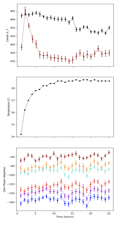
Figure 11: From Top to Bottom: (1) Airy disk centering pixel for the 24 hour data. Red is X, black is Y. The centering pixel corresponds to a correction of the tip-tilt term in the path-length delay. (2) Pick-off mirror temperature. (3) Hole-based gain phase from the self-calibration (20^∘ was added to the gain phase for hole 1 to avoid overlap; 1=dark red, 2=red, 3=orange, 4=turquoise, blue=5, violet=6).

7 Discussion

7.1 Full complex visibility self-calibration, imaging, and deconvolution

We have shown that iterative complex self-calibration and model optimization starting from a point source model, converges on the correct Gaussian beam shape at ALBA. We have further shown that a Fourier imaging and PSF deconvolution process using the self-calibrated visibilities recovers much of the source structure accurately (major axis size and position angle). These results are encouraging for future characterization of more complex sources with non-Gaussian morphologies using masking interferometric imaging, deconvolution, and self-calibration, as may be the case for free electron lasers [24, 25], and for the core-halo problem in some particle accelerators [38].

Interferometric self-calibration and imaging has long been used with radio astronomical interferometers, even for very complex sources [39, 6, 8, 40]. While these techniques were known to optical astronomers employing interferometry, self-calibration techniques have not been used in optical astronomical interferometry because of the very low signal to noise per visibility per coherence time (typically a few source photons per coherence time, even for large apertures [41]).

There has been an application of masking interferometry including visibility phases in the context of alignment of mirrors in a segmented mirror telescope, [42]. However, this technique focused on mirror tilt and piston alignment based principally on phase structure across individual $u,v$ samples, with fine piston tuning using visibility mean phase. The technique does not entail a full complex Fourier analysis including joint solution for both source structure and the complex gains of the individual interferometer elements.

As for laboratory optical interferometry with very bright sources, such as with synchrotron light sources where each exposure frame may contain millions of photons, it is unclear why full complex self-calibration has never been considered, but we note that most previous analyses involved sinusoidal fringe fitting in the image plane (the native measurement space for the optical measurements), to derive visibility coherences from the relative strength of the fringe peak to the first trough, along the lines first employed in the Michelson stellar interferometer in 1891 [43]. Consideration of element-based self-calibration in the Fourier conjugate voltage plane (the native measurement space that allows for self-calibration), has never been adopted, as far as we know.

7.2 Wavefront sensing

We have considered the gain phase solutions from self-calibration in the context of wavefront sensing in an optical system. The gain phases reflect path-length delays through the system for the wavefront along different rays to the aperture. Using both visibility phase time series, as well as the gain phase solutions, we have shown there is delay jitter on short timescales (likely of order milliseconds), at the level of tens of degrees in phase or tens of nanometers in path-length. For the visibilities this phase jitter correlates between neighboring baselines, and for phase gains the jitter correlates between neighboring holes. This jitter is likely dominated by vibration in the optics, with a contribution by laboratory turbulence. The residual visibility phase jitter after calibration is more noise-like (uncorrelated), and much lower than before calibration, implying that the vibration-induced phase variations are being measured with high signal-to-noise. Such short timescale measurements, which we have made with a frame exposure time of 0.3 ms, could be employed as part of an adaptive optics system with much higher frame rate.

We have also demonstrated long timescale delays (hours), likely reflecting slow flexure of the optical components. This flexure appears to be at the level of tens up to a few hundred nanometers. Such slow, or static, path-length delay measurements are relevant to surface metrology and optometry.

Unfortunately, none of our tests demonstrate a quantitative relationship between a known path-length delay and the measured gain phase solutions. Such a demonstration awaits a proper test by inserting a deformable mirror into the optical path that can be calibrated with a known wavefront distortion. The goal would be to recover the path-length distortion through self-calibration via the gain phase measurements. Such tests are being considered, but currently beyond our laboratory apparatus. However, we note that the quantitative relationship between self-calibration complex phase gains and path-length delays has been amply demonstrated in radio astronomical interferometry [44, 45, 6].

This paper represent a first consideration of the concept of using self-calibration phase gains as a wavefront sensor in optical masking interferometry. We briefly compare some of the limitations of this self-calibration approach with industry standard SHWFS, in terms of precision and dynamic range.

In terms of precision, the smallest wavefront distortion measurable by a SHWFS is essentially set by how well a grid spot can be centered relative to the unperturbed grid. The accuracy of centering depends ultimately on the pixel size and the signal to noise. SHWFS have been built with quoted precisions of a few nanometers for path-length delays [46, 30]. Likewise, nanometer precision has been demonstrated with reference wave-type WFS, such as the Talbot WFS [33].

For our self-calibration approach, the precision is set by the accuracy with which the phase gain can be determined by the self-calibration. This accuracy depends principally on the signal-to-noise per visibility. In Figures 8, after calibration the visibility phase rms for the time series is $\sim 1.2^{\circ}$, and it is uncorrelated between baselines. We consider this rms after calibration our empirical estimate of the random (uncorrelated) noise on each visibility phase measurement per frame.

This visibility-based phase noise then sets the noise-floor for the gain phases derived with self-calibration process. In our 7-hole experiment, each gain phase is derived from 6 visibilities, such that we expect the noise on the gain phases to decrease relative to the visibility phase noise by a factor root(6). Hence, the noise-like limit to the gain phase measurements per frame is $\sim 0.5^{\circ}$. At 400 nm, this gain phase rms limit then implies a path-length precision of 0.6 nm.

The dynamic range of a wavefront sensor is defined as the maximum path-length distortion measurable, in units of wavelengths. For a Shack-Hartmann lenslet array, the maximum wavefront tilt per lenslet is set by the need to avoid shifting the source image to the next grid cell. The total dynamic range is then set by the sum of these shifts across the array [31]. SHWFS have now been designed with dynamic ranges in the many hundreds, or even a thousand [47].

For the self-calibration approach, for a single wavelength measurement, the maximum phase change between holes is limited by a phase wrap of $360^{\circ}$, or one wavelength between pairs of holes. One could populate the mask with holes that sample the wavefront incrementally, such that the wraps could be determined, as is done in SHWFS, but that will still only increase the dynamic range to a few wavelengths. However, the dynamic range can be greatly enhanced by adding a frequency axis to the analysis. Gain phases for a physical path-length distortion are linear in wavelength, so making a closely spaced measurement in frequency can determine the phase wraps. For example, making two measurements of the phase screen separated in wavelength by 5% would increase the dynamic range by factor 20 relative to a single measurement.

Using the frequency axis to determine phase wraps is a well known technique in radio Very Long Baseline interferometry, where interference fringes are generated between antennas separated by 10,000 km, or more for space VLBI. VLBI fringe fitting determines path-length delays directly, without resorting to gain phases, by using spectral measurements with fine frequency channel resolution. Linear fits to the phase slope with frequency then determine the path-length delay. This technique is know as ’global fringe fitting’, in which all the visibility spectra are incorporated into a least squares, or other, optimization approach to derive factorizable delays for each interferometric element [45, 48].

A final limitation of self-calibration as a wavefront sensor using a non-redundant mask is that the sampling of the aperture plane, or wavefront, is necessarily sparse in order to maintain non-redundancy to avoid decoherence. For comparison, the SHWSF has a fairly complete sampling of the aperture plane, besides the edges of the lenslets. However, there should be methods to increase the aperture plane sampling for the interferometric masking technique. First, a mask could be designed with much better coverage of the aperture, even close to complete (but necessarily redundant), but then the optics is designed to select out non-redundant subsets of the holes for interferometry through use of optical fibers [49]. Hence, an independent set of non-redundant aperture diffraction images will be created that covers much of the aperture plane. The complication is then tying the ’reference phase’ point between subsets. Tying the reference phase between subsets may require making one hole in common between subsets by using beam splitters.

A second method to improve aperture coverage for the diffraction mask is to use the fact that self-calibration is an over-constrained problem (see Section 3). Hence, partial redundancy might be tolerated for larger N masks, by simply ignoring the redundant samples in the self-calibration solutions. Selecting sub-sets of well sampled $u,v$ data for calibration is a common practice in radio astronomy [8].

Wavefront sensing using self-calibration to determine element-based phases in an interferometer is a demonstrable technique, as employed for decades in radio astronomy. This report represents the first exploration of the technique in laboratory optical interferometry. The technique differs from either reference wave or angle-based WFS in that the path-length delays along each ray are measured directly, relative to the adopted reference point in the aperture. We are considering the relative merits or disadvantages of this technique versus existing techniques. These will likely depend strongly on application.

Acknowledgments. The National Radio Astronomy Observatory is a facility of the National Science Foundation operated under cooperative agreement by Associated Universities, Inc.. Image processing was performed using the Software: Astronomical Image Processing System (AIPS) [50] and Common Astronomical Software Applications (CASA) [20]. Related patents and patent applications: Patent No. US 12,104,901 B2; Provisional Patent No. No. 63/355,174 (RL 8127.032.USPR); Provisional Patent No. 63/648,303 (RL 8127.306.USPR).

Disclosure Statement: The authors declare no conflicts of interest.

Data availability: The ALBA interferograms underlying the results presented in this paper are not publicly available at this time but may be obtained from the authors upon reasonable request.

References

- [1] T. M. Mitsuhashi, “Recent Trends in Beam Size Measurements using the Spatial Coherence of Visible Synchrotron Radiation,” in Proceedings of the 6th International Particle Accelerator Conference, (2015), Proceedings of IPAC.
- [2] L. Torino and U. Iriso, “Transverse beam profile reconstruction using synchrotron radiation interferometry,” \JournalTitlePhys. Rev. Accel. Beams 19, 122801 (2016).
- [3] A. C. S. Readhead, T. S. Nakajima, T. J. Pearson, G. Neugebauer, J. B. Oke, and W. L. W. Sargent, “Diffraction-Limited Imaging with Ground-Based Optical Telescopes,” \JournalTitleAJ 95, 1278 (1988).
- [4] B. Nikolic, C. L. Carilli, N. Thyagarajan, L. Torino, and U. Iriso, “Two-dimensional synchrotron beam characterization from a single interferogram,” \JournalTitlePhysical Review Accelerators and Beams 27, 112802 (2024).
- [5] U. Iriso, L. Torino, C. Carilli, B. Nikolic, and N. Thyagarajan, “New interferometric aperture masking technique for full transverse beam characterization using synchrotron radiation,” \JournalTitlearXiv e-prints arXiv:2409.11135 (2024).
- [6] A. R. Thompson, J. M. Moran, and J. Swenson, George W., Interferometry and Synthesis in Radio Astronomy, 3rd Edition (Springer, Cham, 2017).
- [7] N. Thyagarajan, B. Nikolic, C. L. Carilli, , L. Torino, and U. Iriso, “Two-dimensional Synchrotron Beam Shape Characterization using Interferometric Closure Amplitudes,” \JournalTitlein-prep (2025).
- [8] T. Cornwell and E. B. Fomalont, “Self-Calibration,” in Synthesis Imaging in Radio Astronomy II, vol. 180 of Astronomical Society of the Pacific Conference Series G. B. Taylor, C. L. Carilli, and R. A. Perley, eds. (1999), p. 187.
- [9] T. J. Pearson and A. C. S. Readhead, “Image Formation by Self-Calibration in Radio Astronomy,” \JournalTitleAnnual Reviews of Astronomy and Astrophysics 22, 97–130 (1984).
- [10] A. C. S. Readhead and P. N. Wilkinson, “The mapping of compact radio sources from VLBI data.” \JournalTitleApJ 223, 25–36 (1978).
- [11] F. R. Schwab, “Robust Solution for Antenna Gains,” \JournalTitleNRAO VLA Scientific Memoranda 136 (1981).
- [12] P. H. van Cittert, “Die Wahrscheinliche Schwingungsverteilung in Einer von Einer Lichtquelle Direkt Oder Mittels Einer Linse Beleuchteten Ebene,” \JournalTitlePhysica 1, 201–210 (1934).
- [13] F. Zernike, “The concept of degree of coherence and its application to optical problems,” \JournalTitlePhysica 5, 785–795 (1938).
- [14] M. Born and E. Wolf, Principles of Optics (1999).
- [15] F. R. Schwab, “Processing of three-dimensional data,” in 1980 International Optical Computing Conference I, vol. 231 of Society of Photo-Optical Instrumentation Engineers (SPIE) Conference Series W. T. Rhodes, ed. (1980), p. 18.
- [16] T. J. Cornwell and P. N. Wilkinson, “A new method for making maps with unstable radio interferometers,” \JournalTitleMNRAS 196, 1067–1086 (1981).
- [17] L. Torino and U. Iriso, “Transverse beam profile reconstruction using synchrotron radiation interferometry,” \JournalTitlePhys. Rev. Accel. Beams 19, 122801 (2016).
- [18] A. Sivaramakrishnan, P. Tuthill, J. P. Lloyd, A. Z. Greenbaum, D. Thatte, R. A. Cooper, T. Vandal, J. Kammerer, J. Sanchez-Bermudez, B. J. S. Pope, D. Blakely, L. Albert, N. J. Cook, D. Johnstone, A. R. Martel, K. Volk, A. Soulain, É. Artigau, D. Lafrenière, C. J. Willott, S. Parmentier, K. E. S. Ford, B. McKernan, M. B. Vila, N. Rowlands, R. Doyon, M. Beaulieu, L. Desdoigts, A. W. Fullerton, M. De Furio, P. Goudfrooij, S. T. Holfeltz, S. LaMassa, M. Maszkiewicz, M. R. Meyer, M. D. Perrin, L. Pueyo, J. Sahlmann, S. T. Sohn, P. S. Teixeira, and S.-h. Zheng, “The Near Infrared Imager and Slitless Spectrograph for the James Webb Space Telescope. IV. Aperture Masking Interferometry,” \JournalTitlePublication of the Astronomical Society of the Pacific 135, 015003 (2023).
- [19] E. B. Fomalont, “Image Analysis,” in Synthesis Imaging in Radio Astronomy II, vol. 180 of Astronomical Society of the Pacific Conference Series G. B. Taylor, C. L. Carilli, and R. A. Perley, eds. (1999), p. 301.
- [20] J. P. McMullin, B. Waters, D. Schiebel, W. Young, and K. Golap, “CASA Architecture and Applications,” in Astronomical Data Analysis Software and Systems XVI, vol. 376 of Astronomical Society of the Pacific Conference Series R. A. Shaw, F. Hill, and D. J. Bell, eds. (2007), p. 127.
- [21] B. G. Clark, “An efficient implementation of the algorithm ’CLEAN’,” \JournalTitleAstronomy & Astrophysics 89, 377 (1980).
- [22] J. A. Högbom, “Aperture Synthesis with a Non-Regular Distribution of Interferometer Baselines,” \JournalTitleAstronomy & Astrophysics Supplement 15, 417 (1974).
- [23] T. Cornwell, R. Braun, and D. S. Briggs, “Deconvolution,” in Synthesis Imaging in Radio Astronomy II, vol. 180 of Astronomical Society of the Pacific Conference Series G. B. Taylor, C. L. Carilli, and R. A. Perley, eds. (1999), p. 151.
- [24] Y. Kayser, S. Rutishauser, T. Katayama, T. Kameshima, H. Ohashi, U. Flechsig, M. Yabashi, and C. David, “Shot-to-shot diagnostic of the longitudinal photon source position at the spring-8 angstrom compact free electron laser by means of x-ray grating interferometry,” \JournalTitleOpt. Lett. 41, 733–736 (2016).
- [25] M. Schneider, C. M. Günther, B. Pfau, F. Capotondi, M. Manfredda, M. Zangrando, N. Mahne, L. Raimondi, E. Pedersoli, D. Naumenko, and S. Eisebitt, “In situ single-shot diffractive fluence mapping for x-ray free-electron laser pulses,” \JournalTitleNature Communications 9 (2018).
- [26] J. M. Geary, Introduction to Wavefront Sensors, vol. 18 of Tutorial Texts in Optical Engineering (SPIE Press, 1995).
- [27] R. Davies and M. Kasper, “Adaptive Optics for Astronomy,” \JournalTitleAnnual Reviews of Astronomy and Astrophysics 50, 305–351 (2012).
- [28] C. R. Forest, C. R. Canizares, D. R. Neal, M. McGuirk, and M. L. Schattenburg, “Metrology of thin transparent optics using Shack-Hartmann wavefront sensing,” \JournalTitleOptical Engineering 43, 742-753 (2004).
- [29] R. R. Rammage, D. R. Neal, and R. J. Copland, “Application of Shack-Hartmann wavefront sensing technology to transmissive optic metrology,” in Advanced Characterization Techniques for Optical, Semiconductor, and Data Storage Components, vol. 4779 A. Duparré and B. Singh, eds., International Society for Optics and Photonics (SPIE, 2002), pp. 161 – 172.
- [30] D. R. Neal, J. Copland, and D. A. Neal, “Shack-Hartmann wavefront sensor precision and accuracy,” in Advanced Characterization Techniques for Optical, Semiconductor, and Data Storage Components, vol. 4779 A. Duparré and B. Singh, eds., International Society for Optics and Photonics (SPIE, 2002), pp. 148 – 160.
- [31] J. Liang, B. Grimm, S. Goelz, and J. F. Bille, “Objective measurement of wave aberrations of the human eye with the use of a hartmann–shack wave-front sensor,” \JournalTitleJ. Opt. Soc. Am. A 11, 1949–1957 (1994).
- [32] S. Yi, J. Xiang, M. Zhou, Z. Wu, L. Yang, and Z. Yu, “Angle-based wavefront sensing enabled by the near fields of flat optics,” \JournalTitleNature Communications 12, 6002 (2021).
- [33] Y. Liu, M. Seaberg, D. Zhu, J. Krzywinski, F. Seiboth, C. Hardin, D. Cocco, A. Aquila, B. Nagler, H. J. Lee, S. Boutet, Y. Feng, Y. Ding, G. Marcus, and A. Sakdinawat, “High-accuracy wavefront sensing for x-ray free electron lasers,” \JournalTitleOptica 5, 967–975 (2018).
- [34] M. Mansuripur, The Shack–Hartmann wavefront sensor (Cambridge University Press, 2009), p. 624–631.
- [35] M. Vacalebre, R. Frison, C. Corsaro, F. Neri, S. Conoci, E. Anastasi, M. C. Curatolo, and E. Fazio, “Advanced optical wavefront technologies to improve patient quality of vision and meet clinical requests,” \JournalTitlePolymers 14 (2022).
- [36] C. Carilli, B. Nikolic, L. Torino, U. Iriso, and N. Thyagarajan, “Deriving the size and shape of the ALBA synchrotron light source with optical aperture masking: technical choices,” Tech. rep., ALBA, arXiv:2406.02114 (2024).
- [37] L. Torino, “Longitudinal and Transverse Beam Diagnostic using Synchrotron Radiation at ALBA,” Ph.D. thesis, U. Pisa (main) (2017).
- [38] A. Gorzawski, R. B. Appleby, M. Giovannozzi, A. Mereghetti, D. Mirarchi, S. Redaelli, B. Salvachua, G. Stancari, G. Valentino, and J. F. Wagner, “Probing lhc halo dynamics using collimator loss rates at 6.5 tev,” \JournalTitlePhys. Rev. Accel. Beams 23, 044802 (2020).
- [39] R. A. Perley, “High Dynamic Range Imaging,” in Synthesis Imaging in Radio Astronomy II, vol. 180 of Astronomical Society of the Pacific Conference Series G. B. Taylor, C. L. Carilli, and R. A. Perley, eds. (1999), p. 275.
- [40] R. A. Perley, J. W. Dreher, and J. J. Cowan, “The jet and filaments in Cygnus A.” \JournalTitleAstrophysical Journal Letters 285, L35–L38 (1984).
- [41] D. F. Buscher, Practical optical interferometry: imaging at visible and infrared wavelengths, Cambridge observing handbooks for research astronomers (Cambridge University Press, Cambridge, 2015).
- [42] A. C. Cheetham, N. Cvetojevic, A. Sivaramakrishnan, B. Norris, and P. G. Tuthill, “Fizeau interferometric cophasing of segmented mirrors,” in Space Telescopes and Instrumentation 2014: Optical, Infrared, and Millimeter Wave, vol. 9143 of Society of Photo-Optical Instrumentation Engineers (SPIE) Conference Series J. M. Oschmann, Jr., M. Clampin, G. G. Fazio, and H. A. MacEwen, eds. (2014), p. 914352.
- [43] A. A. Michelson, “Visibility of Interference-Fringes in the Focus of a Telescope,” \JournalTitlePublication of the Astronomical Society of the Pacific 3, 217–220 (1891).
- [44] L. T. Maud, R. P. J. Tilanus, T. A. van Kempen, M. R. Hogerheijde, M. Schmalzl, I. Yoon, Y. Contreras, M. C. Toribio, Y. Asaki, W. R. F. Dent, E. Fomalont, and S. Matsushita, “Phase correction for ALMA. Investigating water vapour radiometer scaling: The long-baseline science verification data case study,” \JournalTitleAstronomy & Astrophysics 605, A121 (2017).
- [45] R. C. Walker, “Very Long Baseline Interferometry,” in Synthesis Imaging in Radio Astronomy II, vol. 180 of Astronomical Society of the Pacific Conference Series G. B. Taylor, C. L. Carilli, and R. A. Perley, eds. (1999), p. 433.
- [46] B. R. Adapa, “The application of wavefront sensing methods to optical surface metrology,” Theses, Université Grenoble Alpes [] (2020).
- [47] M. Lombardo and G. Lombardo, “New methods and techniques for sensing the wave aberrations of human eyes,” \JournalTitleClinical and Experimental Optometry 92, 176–186 (2009).
- [48] F. Schwab and W. Cotton, “Global fringe search techniques for vlbi,” \JournalTitleThe Astronomical Journal 88, 688–694 (1983).
- [49] R. Bacon, M. Accardo, L. Adjali, H. Anwand, S. Bauer, I. Biswas, J. Blaizot, D. Boudon, S. Brau-Nogue, J. Brinchmann, P. Caillier, L. Capoani, C. M. Carollo, T. Contini, P. Couderc, E. Daguisé, S. Deiries, B. Delabre, S. Dreizler, J. Dubois, M. Dupieux, C. Dupuy, E. Emsellem, T. Fechner, A. Fleischmann, M. François, G. Gallou, T. Gharsa, A. Glindemann, D. Gojak, B. Guiderdoni, G. Hansali, T. Hahn, A. Jarno, A. Kelz, C. Koehler, J. Kosmalski, F. Laurent, M. Le Floch, S. J. Lilly, J. L. Lizon, M. Loupias, A. Manescau, C. Monstein, H. Nicklas, J. C. Olaya, L. Pares, L. Pasquini, A. Pécontal-Rousset, R. Pelló, C. Petit, E. Popow, R. Reiss, A. Remillieux, E. Renault, M. Roth, G. Rupprecht, D. Serre, J. Schaye, G. Soucail, M. Steinmetz, O. Streicher, R. Stuik, H. Valentin, J. Vernet, P. Weilbacher, L. Wisotzki, and N. Yerle, “The MUSE second-generation VLT instrument,” in Ground-based and Airborne Instrumentation for Astronomy III, vol. 7735 of Society of Photo-Optical Instrumentation Engineers (SPIE) Conference Series I. S. McLean, S. K. Ramsay, and H. Takami, eds. (2010), p. 773508.
- [50] E. W. Greisen, AIPS, the VLA, and the VLBA (2003), vol. 285, p. 109.