Synthesis with Guided Environments

Abstract

In the synthesis problem, we are given a specification, and we automatically generate a system that satisfies the specification in all environments. We introduce and study synthesis with guided environments (SGE, for short), where the system may harness the knowledge and computational power of the environment during the interaction. The underlying idea in SGE is that in many settings, in particular when the system serves or directs the environment, it is of the environment’s interest that the specification is satisfied, and it would follow the guidance of the system. Thus, while the environment is still hostile, in the sense that the system should satisfy the specification no matter how the environment assigns values to the input signals, in SGE the system assigns values to some output signals and guides the environment via programs how to assign values to other output signals. A key issue is that these assignments may depend on input signals that are hidden from the system but are known to the environment, using programs like “copy the value of the hidden input signal $x$ to the output signal $y$.” SGE is thus particularly useful in settings where the system has partial visibility.

We solve the problem of SGE, show its superiority with respect to traditional synthesis, and study theoretical aspects of SGE, like the complexity (memory and domain) of programs used by the system, as well as the connection of SGE to synthesis of (possibly distributed) systems with partial visibility.

I Introduction

Synthesis is the automated construction of a system from its specification [1]. Given a linear temporal logic (LTL) formula $\varphi$ over sets $I$ and $O$ of input and output signals, the goal is to return a transducer that realizes $\varphi$. At each moment in time, the transducer reads a truth assignment, generated by the environment, to the signals in $I$, and generates a truth assignment to the signals in $O$. This process continues indefinitely, generating an infinite computation in $(2^{I\cup O})^{\omega}$. The transducer realizes $\varphi$ if its interactions with all environments generate computations that satisfy $\varphi$ [2].

The fact the system has to satisfy its specification in all environments has led to a characterization of the environment as hostile. In particular, in the game that corresponds to synthesis, the objective of the environment is to violate the specification $\varphi$. In real-life applications, the satisfaction of the specification is often also in the environment’s interest. In particular, in cases where the system serves or guides the environment, we can expect the environment to follow guidance from the system. We introduce and study synthesis with guided environments (SGE, for short), where the system may harness the knowledge and computational power of the environment during the interaction, guiding it how to assign values to some of the output signals.

Specifically, in SGE, the set $O$ of output signals is partitioned into sets $C$ and $G$ of controlled and guided signals. Then, a system that is synthesized by SGE assigns values to the signals in $C$ and guides the environment how to assign values to the signals in $G$. Clearly, not all output signals may be guided to the environment. For example, physical actions of the system, like closing a gate or raising a robot arm, cannot be performed by the environment. In addition, it may be the case that the system cannot trust the environment to follow its guidance. As argued above, however, in many cases we can expect the environment to follow the system’s guidance, and require the system to satisfy the specification only when the environment follows its guidance. Indeed, when we go to the cinema and end up seeing a bad movie, we cannot blame a recommendation system that guided us not to choose this movie. The recommendation system is bad (violates its specification, in our synthesis story) only if a user that follows its guidance is disappointed.

One advantage of SGE is that it enables a decomposition of the satisfaction task between the system and the environment. We will get back to this point after we describe the setting in more detail. The main advantage of SGE, however, has to do with partial visibility, namely the setting where the set $I$ of input signals is partitioned into sets $V$ and $H$ of visible and hidden signals, and the systems views only the signals in $V$. Partial visibility makes synthesis much harder, as the hidden signals still appear in the specification, yet the behavior of the system should be independent of their truth values.

Synthesis with partial visibility has been the subject of extensive research. One line of work studies the technical challenges in solving the problem [5, 6, 7]. Essentially, in a setting with full visibility, the interaction between the system and the environment induces a single computation and hence a single run of a deterministic automaton for the specification. Partial visibility forces the algorithm to maintain subsets of states of the automaton. Indeed, now the interaction induces several computations, obtained by the different possible assignments to the hidden signals. This makes synthesis with partial visibility exponentially harder than synthesis with full visibility for specifications given by automata. When the specification is given by an LTL formula, this exponential price is dominated by the doubly-exponential translation of LTL formulas to deterministic automata, thus LTL synthesis with partial visibility is 2EXPTIME-complete, and is not harder than LTL synthesis with full visibility [8].

A second line of work studies different settings in which partial visibility is present. This includes, for example, distributed systems [9, 10, 11], systems with controlled sensing [12, 13] or with assumptions about visibility [14], and systems that maintain privacy [15, 16]. Finally, researchers have studied alternative forms of partial visibility (e.g., perspective games, where visibility of all signals is restricted in segments of the interaction), as well as partial visibility in richer settings (e.g., multi-agent [17, 18, 19] or stochastic [20, 21] systems) or in problems that are strongly related to synthesis (e.g., control [22], planning [23], and rational synthesis [24, 25]).

To the best of our knowledge, in all settings in which synthesis with partial visibility has been studied so far, there is no attempt to make use of the fact that the assignments to the hidden signals are known to the environment. In SGE, the guidance that the system gives the environment may refer to the values of the hidden signals. Thus, the outcome of SGE is a transducer with a guided environment (TGE): a transducer whose transitions depend only on the assignments to the signals in $V$, it assigns values to the signals in $C$, and guides the environment how to assign values to the signals in $G$ using programs that may refer to the values of the signals in $H$.

Consider, for example, a system in a medical clinic that directs patients “if you come for a vaccine, go to the first floor; if you come to the pharmacy, go to the second floor”. Such a system is as correct as a system that asks customers for the purpose of their visit and then outputs the floor to which they should go. Clearly, if the customers prefer not to reveal the purpose of their visit, we can direct them only with a system of this type. This is exactly what SGE does: it replaces assignments that depend on hidden signals or are complicated to compute with instructions to the environment. As another example, consider a smart-home controller that manages various smart devices within a home by getting inputs from devices like thermostats and security cameras, and generating outputs to devices like lighting systems or smart locks. When it is desirable to hide from the controller information like sleep patterns or number of occupants, we can do that by limiting its input, and guiding the user about the activation of some output devices, for example with instructions like, “if you expect guests, unlock the backyard gate”. In Examples II.1 and II.2, we describe more elaborated examples, in particular of a server that directs users who want to upload data to a cloud. The users may hide from the server the sensitivity level of their data, and we can expect them to follow instructions that the server issues, for example instructions to use storage of high security only when the data they upload is sensitive.

We study several aspects of SGE. We start by examining the memory used by the environment. Clearly, this memory can be used to reduce the state space of the TGE. To see this, note that in an extreme setting in which the TGE can guide all output signals, it can simply instruct the environment to execute a transducer that realizes the specification. Beyond a trade-off between the size of the TGE and the memory of the environment, we discuss how the size of the memory depends on the sets of visible and guided signals. For example, we show that, surprisingly, having more guided signals does not require more memory, yet having fewer guided signals may require more memory.

We then describe an automata-based solution for SGE. The main challenge in SGE is as follows. Consider a system that views only input signals in $V$. Its interactions with environments that agree on the signals in $V$ generate the same response. In synthesis with partial visibility, this is handled by universal tree automata that run on trees with directions in $2^{V}$, thus trees whose branches correspond to the interaction from the point of view of the system [6]. In the setting of SGEs, the interactions with different environments that agree on the signals in $V$ still generate the same response, but this response now involves programs that guide the environment on how to assign values to signals in $G$ based on the values assigned to the signals in $H$. As a result, the computations induced by these interactions may differ (not only on $H$ but also on $G$). This differences between SGE and traditional synthesis with partial visibility is our main technical challenge. We show that we can still reduce SGE to the nonemptiness problem of universal co-Büchi tree automata, proving that SGE for LTL specifications is 2EXPTIME-complete. In more detail, given an LTL formula $\varphi$ and a bound $k$ on the memory that the environment may use, the constructed automaton is of size exponential in $|\varphi|$ and linear in $k$, making SGE doubly-exponential in $|\varphi|$ and exponential in $k$. Finally, we prove a doubly-exponential upper bound on the size of the memory needed by the environment, leading to an overall triply-exponential upper bound for the SGE problem with unbounded environment memory.

We continue and study the domain of programs that TGEs use. Recall that these programs guides the environment how to update its memory and assign values to the guided signals, given a current memory state and the current assignment to the hidden signals. Thus, for a memory state space $M$, each program is of the form $p:M\times 2^{H}\rightarrow M\times 2^{G}$. We study ways to reduce the domain $2^{H}$, which is the most dominant factor. The reduction depends on the specification $\varphi$ we wish to synthesize. We argue that the SGE algorithm can restrict attention to tight programs: ones whose domain is a set of predicates over $H$ obtained by simplifying propositional sub-formulas of $\varphi$. Further simplification is achieved by exploiting the fact that programs are called after an assignment to the signals in $V\cup C$ has been fixed, and exploiting dependencies among all signals.

Finally, we compare our solution with one that views a TGE as two distributed processes that are executed together in a pipeline architecture: the TGE itself, and a transducer with state space $M$ that implements the instructions of the TGE to the environment. We argue that the approach we take is preferable and can lead to a quadratic saving in their joint state spaces, similar to the saving obtained by defining a regular language as the intersection of two automata. Generating programs that manage the environment’s memory efficiently is another technical challenge in SGE.

We conclude with directions for future research. Beyond extensions of the many settings in which synthesis has been studied to a setting with guided environments, we discuss two directions that are more related to “the guided paradigm” itself: settings with dynamic hiding and guidance of signals, thus when $H$ and $G$ are not fixed throughout the interaction; and bounded SGE, where, as in traditional synthesis [26, 27], beyond a bound on the memory used by the environment, there are bounds on the size of the state space of the TGE and possibly also on the size of the state space of its environment.

II Preliminaries

We describe on-going behaviors of reactive systems using the linear temporal logic LTL [28]. We consider systems that interact via sets $I$ and $O$ of input and output signals, respectively. Formulas of LTL are defined over $I\cup O$ using the usual Boolean operators and the temporal operators $\mathbf{G}$ (“always”) and $\mathbf{F}$ (“eventually”), $\mathbf{X}$ (“next time”) and $\mathbf{U}$ (“until”). The semantics of LTL is defined with respect to infinite computations in $(2^{I\cup O})^{\omega}$. Thus, each LTL formula $\varphi$ over $I\cup O$ induces a language $L_{\varphi}\subseteq(2^{I\cup O})^{\omega}$ of all computations that satisfy $\varphi$.

The length of an LTL formula $\varphi$, denoted $|\varphi|$, is the number of nodes in the generating tree of $\varphi$. Note that $|\varphi|$ bounds the number of sub-formulas of $\varphi$.

We model reactive systems that interact with their environments by finite-state transducers. A transducer is a tuple $\hskip 1.5pt{\mathcal{T}}=\langle I,O,S,s_{0},\delta,\tau\rangle$, where $I$ and $O$ are sets of input and output signals, $S$ is a finite set of states, $s_{0}\in S$ is an initial state, $\delta:S\times 2^{I}\rightarrow S$ is a transition function, and $\tau:S\times 2^{I}\rightarrow 2^{O}$ is a function that labels each transition by an assignment to the output signals. Given an infinite sequence $w_{I}=i_{1}\cdot i_{2}\cdots\in(2^{I})^{\omega}$ of assignments to input signals, $\hskip 1.5pt{\mathcal{T}}$ generates an infinite sequence $w_{O}=o_{1}\cdot o_{2}\cdots\in(2^{O})^{\omega}$ of assignments to output signals. Formally, a run of $\hskip 1.5pt{\mathcal{T}}$ on $w_{I}$ is an infinite sequence of states $s_{0}\cdot s_{1}\cdot s_{2}\cdots$, where for all $j\geq 1$, we have that $s_{j}=\delta(s_{j-1},i_{j})$. Then, the sequence $w_{O}$ is obtained from the assignments along the transitions that the run traverses. Thus for all $j\geq 1$, we have that $o_{j}=\tau(s_{j-1},i_{j})$. We define the computation of $\hskip 1.5pt{\mathcal{T}}$ on $w_{I}$ to be the word $\hskip 1.5pt{\mathcal{T}}(w_{I})=(i_{1}\cup o_{1})\cdot(i_{2}\cup o_{2})\cdots\in(2^{I\cup O})^{\omega}$.

For a specification language $L_{\varphi}\subseteq(2^{I\cup O})^{\omega}$, we say that $\hskip 1.5pt{\mathcal{T}}$ $(I,O)$-realizes $L_{\varphi}$ if for every input sequence $w_{I}\in(2^{I})^{\omega}$, we have that $\hskip 1.5pt{\mathcal{T}}(w_{I})\in L_{\varphi}$. In the synthesis problem, we are given a specification language $L_{\varphi}$ and a partition of the signals to $I$ and $O$, and we have to return a transducer that $(I,O)$-realizes $L_{\varphi}$ (or determine that $L_{\varphi}$ is not realizable). The language $L_{\varphi}$ is typically given by an LTL formula $\varphi$. We then talk about realizability or synthesis of $\varphi$ (rather than $L_{\varphi}$).

In synthesis with partial visibility, we seek a system that satisfies a given specification in all environments even when it cannot observe the assignments to some of the input signals. Formally, the set of input signals is partitioned into visible and hidden signals, thus $I=V\cup H$. The specification $\varphi$ is still over $V\cup H\cup O$, yet the behavior of the transducer that models the system is independent of $H$. Formally, $\hskip 1.5pt{\mathcal{T}}=\langle V,H,O,S,s_{0},\delta,\tau\rangle$, where now $\delta:S\times 2^{V}\rightarrow S$ and $\tau:S\times 2^{V}\rightarrow 2^{O}$. Given an infinite sequence $w_{I}=(v_{1}\cup h_{1})\cdot(v_{2}\cup h_{2})\cdots\in(2^{V\cup H})^{\omega}$, the run and computation of $\hskip 1.5pt{\mathcal{T}}$ on $w_{I}$ is defined as in the case of full visibility, except that now, for all $j\geq 1$, we have that $s_{j}=\delta(s_{j-1},v_{j})$ and $o_{j}=\tau(s_{j-1},v_{j})$.

We can now define a transducer with a guided environment (TGE for short). TGEs extend traditional transducers by instructing the environment how to manage its guided signals. A TGE may be executed in a setting with partial visibility, thus $I=V\cup H$. It uses the fact that the assignments to the signals in $H$ are known to the environment, and it guides the assignment to some of the output signals to the environment. As discussed in Section I, in practice not all output signals can be guided. Formally, the set of output signals is partitioned into controlled and guided signals, thus $O=C\cup G$. In each transition, the TGE assigns values to the signals in $C$ and instructs the environment how to assign values to the signals in $G$. The environment may have a finite memory, in which case the transducer also instructs the environment how to update the memory in each transition. The instructions that the transducer generates are represented by programs, defined below.

Consider a finite set $M$ of memories, and sets $H\subseteq I$ and $G\subseteq O$ of input and output signals. Let $\mathcal{P}_{M,H,G}=(M\times 2^{G})^{M\times 2^{H}}$ denote the set of propositional programs that update the memory state and assign values to signals in $G$, given a memory in $M$ and an assignment to the signals in $H$. Note that each member of $\mathcal{P}_{M,H,G}$ is of the form $p:M\times 2^{H}\rightarrow M\times 2^{G}$. For a program $p\in\mathcal{P}_{M,H,G}$, let $p_{M}:M\times 2^{H}\rightarrow M$ and $p_{G}:M\times 2^{H}\rightarrow 2^{G}$ be the projections of $p$ onto $M$ and $G$ respectively. Thus, $p(m,h)=\langle p_{M}(m,h),p_{G}(m,h)\rangle$ for all $\langle m,h\rangle\in M\times 2^{H}$. In Section V we discuss ways to restrict the set of programs that a TGE may suggest to its environment without affecting the outcome of the synthesis procedure.

Now, a TGE is $\hskip 1.5pt{\mathcal{T}}=\langle V,H,C,G,S,s_{0},\delta,M,m_{0},\tau\rangle$, where $V$ and $H$ are sets of visible and hidden input signals, $C$ and $G$ are sets of controlled and guided output signals, $S$ is a finite set of states, $s_{0}\in S$ is an initial state, $\delta:S\times 2^{V}\rightarrow S$ is a transition function, $M$ is a set of memories that the environment may use, $m_{0}\in M$ is an initial memory, and $\tau:S\times 2^{V}\rightarrow 2^{C}\times\mathcal{P}_{M,H,G}$ labels each transition by an assignment to the controlled output signals and a program. Note that $\delta$ and $\tau$ are independent of the signals in $H$, and that $\tau$ assigns values to the signals in $C$ and instructs the environment how to use the signals in $H$ in order to assign values to the signals in $G$. The latter reflects the fact that the environment does view the signals in $H$, and constitute the main advantage of TGEs over standard transducers.

Given an infinite sequence $w_{I}=(v_{1}\cup h_{1})\cdot(v_{2}\cup h_{2})\cdots\in(2^{V\cup H})^{\omega}$, the run of $\hskip 1.5pt{\mathcal{T}}$ on $w_{I}$ is obtained by applying $\delta$ on the restriction of $w_{I}$ to $V$. Thus, $r=s_{0}\cdot s_{1}\cdot s_{2}\cdots$, where for all $j\geq 1$, we have that $s_{j}=\delta(s_{j-1},v_{j})$. The interaction of $\hskip 1.5pt{\mathcal{T}}$ with the environment generates an infinite sequence $w_{C}=c_{1}\cdot c_{2}\cdot c_{3}\cdots\in(2^{C})^{\omega}$ of assignments to the controlled signals, an infinite sequence $w_{M}=m_{0}\cdot m_{1}\cdot m_{2}\cdots\in M^{\omega}$ of memories, and an infinite sequence $w_{P}=p_{1}\cdot p_{2}\cdot p_{3}\cdots\in(\mathcal{P}_{M,H,G})^{\omega}$ of programs, which in turn generates an infinite sequence $w_{G}=d_{1}\cdot d_{2}\cdot d_{3}\cdots\in(2^{G})^{\omega}$ of assignments to the guided signals. Formally, for all $j\geq 1$, we have that $\langle c_{j},p_{j}\rangle=\tau(s_{j-1},v_{j})$ and $\langle m_{j},d_{j}\rangle=p_{j}(m_{j-1},h_{j})$. The computation of $\hskip 1.5pt{\mathcal{T}}$ on $w_{I}$ is then $\hskip 1.5pt{\mathcal{T}}(w_{I})=(v_{1}\cup h_{1}\cup c_{1}\cup d_{1})\cdot(v_{2}\cup h_{2}\cup c_{2}\cup d_{2})\cdots\in(2^{V\cup H\cup C\cup G})^{\omega}$.

Note that while the domain of the programs in $\mathcal{P}_{M,H,G}$ is $M\times 2^{H}$, programs are chosen in $\hskip 1.5pt{\mathcal{T}}$ along transitions that depend on $2^{V}$. Thus, effectively, assignments made by programs depend on signals in both $H$ and $V$.

For a specification language $L_{\varphi}\subseteq(2^{I\cup O})^{\omega}$, partitions $I=V\cup H$ and $O=C\cup G$, and a bound $k\geq 1$ on the memory that the environment may use, we say that a TGE $\hskip 1.5pt{\mathcal{T}}$, $(V,H,C,G)$-realizes $L_{\varphi}$ with memory $k$, if $\hskip 1.5pt{\mathcal{T}}=\langle V,H,C,G,S,s_{0},\delta,M,m_{0},\tau\rangle$, with $|M|=k$, and $\hskip 1.5pt{\mathcal{T}}(w_{I})\in L_{\varphi}$, for every input sequence $w_{I}\in(2^{I})^{\omega}$. Then, in the synthesis with guided environment problem (SGE, for short), given such a specification $L_{\varphi}\subseteq(2^{I\cup O})^{\omega}$, a bound $k\geq 1$ and partitions $I=V\cup H$ and $O=C\cup G$, we should construct a TGE with memory $k$ that $(V,H,C,G)$-realizes $L_{\varphi}$ (or determine that no such TGE exists).

Let us consider the special case of TGEs that operate in an environment with no memory, thus $M=\{m\}$, for a single memory state $m$. Consider first the setting where $\hskip 1.5pt{\mathcal{T}}$ has full visibility, thus $V=I$ and $H=\emptyset$. Then, programs are of the form $p:{\{m\}}\times 2^{\emptyset}\rightarrow{\{m\}}\times 2^{G}$, and so each program is a fixed assignment to the signals in $G$. Hence, TGEs that have full visibility and operate in an environment with no memory coincide with traditional transducers. Consider now a setting with partial visibility, thus $V\neq I$. Now, programs are of the form $p:{\{m\}}\times 2^{H}\rightarrow{\{m\}}\times 2^{G}$, allowing the TGE to guide the environment in a way that depends on signals in $H$.

In Examples II.1 and II.2 below, we demonstrate how collaboration from the environment can lead to the realizability of specifications that are otherwise non-realizable.

Example II.1

[TGEs for simple specifications] Let $I=\{i\}$, $O=\{o\}$, and consider the simple specification $\varphi_{1}=\mathbf{G}(i\leftrightarrow o)$. Clearly, $\varphi_{1}$ is realizable in a setting with full visibility, yet is not realizable in a setting with partial visibility and $H=\{i\}$. A TGE can realize $\varphi_{1}$ even in the latter setting. Indeed, even when the environment has no memory, it can delegate the assignment to $o$ to the environment and guide it to copy the value of $i$ into $o$. Formally, $\varphi_{1}$ is realizable by the $\hskip 1.5pt{\mathcal{T}}_{1}=\langle\emptyset,\{i\},\emptyset,\{o\},\{s\},\{s\},\delta,\{m\},m,\tau\rangle$, with $\delta(s,\emptyset)=s$ and $\tau(s,\emptyset)=\langle\emptyset,p\rangle$, where the program $p\in\mathcal{P}_{\{m\},\{i\},\{o\}}$ is the command $o:=i$.

Consider now the specification $\varphi_{2}=\mathbf{G}(i\leftrightarrow\mathbf{X}o)$. Here, a TGE in a setting in which $i$ is not visible needs an environment with at least one register, inducing a memory of size $2$. Then, the TGE can instract the environment to store the value of $i$ in the register, and use the stored value when assigning a value to the signal $o$ in the next round. Formally, $\varphi_{2}$ is realizable by the TGE $\hskip 1.5pt{\mathcal{T}}_{2}=\langle\emptyset,\{i\},\emptyset,\{o\},\{s\},\{s\},\delta,\{m_{0},m_{1}\},m_{0},\tau\rangle$,with $\delta(s,\emptyset)=s$ and $\tau(s,\emptyset)=\langle\emptyset,p\rangle$, where $p\in\mathcal{P}_{\{m_{0},m_{1}\},\{i\},\{o\}}$ instructs the environment to move to $m_{0}$ when $i=\mathtt{F}$ and to $m_{1}$ when $i=\mathtt{T}$, and to assigns $\mathtt{F}$ to $o$ when it is in $m_{0}$ and $\mathtt{T}$ when it is in $m_{1}$. ∎

Example II.2

[A TGE implementing a server] Consider a server that directs users who want to upload data to a cloud. The set of input signals is $I=\{{\it req},{\it sens}\}$, where ${\it req}$ holds when a user requests to upload data, and ${\it sens}$ holds when the data is sensitive. The set of output signals is $O=\{{\it open},{\it high}\}$, where ${\it open}$ holds when the cloud is open for uploading, and ${\it high}$ holds when the storage space is of high security. Users pay more for storage of high security. Therefore, in addition to guaranteeing that all requests are eventually responded by ${\it open}$, we want the server to direct the users to use storage of high security only when the data they upload is sensitive. In addition, the cloud cannot stay always open to uploads. Formally, we want to synthesize a transducer that realizes the conjunction $\varphi$ of the following LTL formulas.

• $\varphi_{1}=\mathbf{G}(({\it req}\wedge{\it sens})\rightarrow((\neg{\it open})\mathbf{U}({\it open}\wedge{\it high})))$.

• $\varphi_{2}=\mathbf{G}(({\it req}\wedge\neg{\it sens})\rightarrow((\neg{\it open})\mathbf{U}(({\it open}\wedge\neg{\it high})\vee({\it req}\wedge{\it sens})))$.

• $\varphi_{3}=\mathbf{G}\mathbf{F}\neg{\it open}$.

A server that has full visibility of $I$ can realize $\varphi$. To see this, note that a server can open the cloud for uploading whenever a request arrives, storing the data in a storage of high security iff it is sensitive. Then, in order to satisfy $\varphi_{3}$, the server should delay the response to successive requests, but this does not prevent it from satisfying $\varphi_{1}$ and $\varphi_{2}$.

Users may prefer not to share with the server information about the sensitivity of their data. In current settings of synthesis with partial visibility, this renders $\varphi$ to be unrealizable. Indeed, when the sensitivity of the data is hidden from the scheduler, thus when $V=\{{\it req}\}$ and $H=\{{\it sens}\}$, the behavior of the server is independent of ${\it sens}$, making it impossible to assign values to ${\it high}$ in a way that satisfies $\varphi$ in all environments.

While the output signal ${\it open}$ controls access to the cloud, the output signal ${\it high}$ only directs the user which type of storage to use, and it is of the user’s interest to store her data in a storage of an appropriate security level. Accordingly, the environment can be guided with the assignment to ${\it high}$. Thus, $C=\{{\it open}\}$ and $G=\{{\it high}\}$.

Figure 1: A transducer with a guided environment.

In Figure 1, we present a TGE that implements such a guidance and realizes $\varphi$. Each transition of the TGE is labeled by a guarded command of the form $v/[c,p]$, where $v\in 2^{V}$ is an assignment to the visible input signals (or a predicate describing several assignments), $c\in 2^{C}$ is an assignment to the controlled output signals, and $p$ is a program that instructs the environment how to assign values to the guided signals and how to update its memory. The environment uses a memory with one register $r$. Accordingly, the transitions of the TGE are guarded by the truth value of ${\it req}$, they include an assignment to ${\it open}$, and then a program that instructs the environment how to assign a value to ${\it high}$ and to the register $r$. The key advantage of TGEs is that these instructions may depend on the hidden input signals. Indeed, the environment does know their values. For example, when the TGE moves from $s_{1}$ to $s_{2}$, it instructs the environment to assign to $r$ the value of ${\it sens}$. Then, when the TGE moves from $s_{2}$ to $s_{1}$, it instructs the environment to use the value stored in $r$ (as well as the current value of ${\it sens}$) when it assigns a value to ${\it high}$. ∎

III On the Memory Used by the Environment

In this section we examine different aspects of the memory used by the environment. We discuss a trade-off between the size of the memory and the size of the TGE, and how the two depend on the partitions $I=V\cup H$ and $O=C\cup G$ of the input and output signals.

Example III.1

In order to better understand the need for memory and the technical challenges around it, consider the tree appearing in Figure 2.

Figure 2: Two rounds of interaction with a TGE $\hskip 1.5pt{\mathcal{T}}$.

The tree describes two rounds of an interaction between a TGE $\hskip 1.5pt{\mathcal{T}}$ and its environment. In both rounds, $\hskip 1.5pt{\mathcal{T}}$ views the assignment $v\in 2^{V}$. Consider two assignments $h_{1},h_{2}\in 2^{H}$. The tree presents the four possible extensions of the interaction by assignments in $\{h_{1},h_{2}\}$. Since the signals in $H$ are hidden, $\hskip 1.5pt{\mathcal{T}}$ cannot distinguish among the different branches of the tree. In particular, it has to suggest to the environment the same program in all the transitions from the root to its successors, and the same program in all the transitions from these successors to the leaves. While these programs may depend on $H$, a program with no memory would issue the same assignment to the signals in $G$ along the two dashed transitions $\langle h_{1},h_{1}.h_{2}\rangle$ and $\langle h_{2},h_{2}.h_{2}\rangle$. Indeed, in both transitions, the environment assigns $h_{2}\in 2^{H}$ to the hidden signals. Using memory, $\hskip 1.5pt{\mathcal{T}}$ can instruct the environment to maintain information about the history of the computation, and thus distinguish between computations with the same visible component and the same current assignment to the hidden signals. For example, by moving to memory state $m_{1}$ with $h_{1}$ and to memory state $m_{2}$ with $h_{2}$, a program may instruct the environment to assign different values along the dashed lines. ∎

We first observe that in settings in which all output signals can be guided, the TGE can instruct the environment to simulate a transducer that realizes the specification. Also, in settings with full visibility, the advantage of guided environments is only computational, thus specifications do not become realizable, yet may be realizable by smaller systems. Formally, we have the following.

Theorem III.2

Consider an LTL specification $\varphi$ over $I\cup O$.

1. If $\varphi$ is realizable by a transducer with $n$ states, then $\varphi$ is $(\emptyset,I,\emptyset,O)$-realizable by a one-state TGE with memory $n$.

2. For every partition $I=V\cup H$ and $O=C\cup G$, if $\varphi$ is $(V,H,C,G)$-realizable by a TGE with $n$ states and memory $k$, then $\varphi$ is $(I,O)$-realizable (in a setting with full visibility) by a transducer with $n\cdot k$ states. In particular, if $\varphi$ is $(\emptyset,I,\emptyset,O)$-realizable by a one-state TGE with memory $k$, then $\varphi$ is $(I,O)$-realizable (in a setting with full visibility) by a transducer with $k$ states.

Proof:

We start with the first claim. Given a transducer $\hskip 1.5pt{\mathcal{T}}=\langle I,O,S,s_{0},\delta,\tau\rangle$, we define a program $p\in\mathcal{P}_{S,I,O}$ that instructs the environment to simulate $\hskip 1.5pt{\mathcal{T}}$. Formally, for every $s\in S$ and $i\in 2^{I}$, we have that $p(s,i)=\langle\delta(s,i),\tau(s,i)\rangle$. Consider the TGE $\hskip 1.5pt{\mathcal{T}}^{\prime}=\langle\emptyset,I,\emptyset,O,\{s\},s,\delta^{\prime},S,s_{0},\tau^{\prime}\rangle$, with $\delta^{\prime}(s,\emptyset)=s$ and $\tau^{\prime}(s,\emptyset)=\langle\emptyset,p\rangle$. It is easy to see that for every $w_{I}\in(2^{I})^{\omega}$, we have that $\hskip 1.5pt{\mathcal{T}}(w_{I})=\hskip 1.5pt{\mathcal{T}}^{\prime}(w_{I})$. In particular, if $\hskip 1.5pt{\mathcal{T}}$ realizes $\varphi$, then so does $\hskip 1.5pt{\mathcal{T}}^{\prime}$.

We continue to the second claim. Note that the special case where $V=C=\emptyset$ is the “only if” direction of the first claim. Given a TGE $\hskip 1.5pt{\mathcal{T}}=\langle V,H,C,G$, $S,s_{0}$, $\delta,M$, $m_{0},\tau\rangle$, consider the transducer $\hskip 1.5pt{\mathcal{T}}^{\prime}=\langle H\cup V,C\cup G,S\times M,\langle s_{0},m_{0}\rangle,\delta^{\prime},\tau^{\prime}\rangle$, where for all $\langle s,m\rangle\in S\times M$ and $i\in 2^{H\cup V}$ with $\tau(s,i\cap H)=\langle c,p\rangle$, we have that $\delta^{\prime}(\langle s,m\rangle,i)=\langle\delta(s,i\cap V),p_{M}(i\cap H)\rangle$ and $\tau^{\prime}(\langle s,m\rangle,i)=c\cup p_{G}(i\cap H)$. It is easy to see that for every $w_{I}\in(2^{I})^{\omega}$, we have that $\hskip 1.5pt{\mathcal{T}}(w_{I})=\hskip 1.5pt{\mathcal{T}}^{\prime}(w_{I})$. In particular, if $\hskip 1.5pt{\mathcal{T}}$ realizes $\varphi$, then so does $\hskip 1.5pt{\mathcal{T}}^{\prime}$. ∎

Note that Theorem III.2 also implies that an optimal balance between controlled and guided signals in a setting with full visibility can achieve at most a quadratic saving in the combined states space of the TGE and its memory. This is similar to the quadratic saving in defining a regular language by the intersection of two automata. Indeed, handling of two independent specifications can be partitioned between the TGE and the environment. Formally, we have the following.

Theorem III.3

For all $\,k\geq 1$, there exists a specification $\varphi_{k}$ over $I={\{i_{1},i_{2}\}}$ and $O={\{o_{1},o_{2}\}}$, such that $\varphi_{k}$ is $({\{i_{1}\}},{\{i_{2}\}},{\{o_{1}\}},{\{o_{2}\}})$-realizable by a TGE with $k$ states and memory $k$, yet a transducer that $(I,O)$-realizes $\varphi_{k}$ needs at least $k^{2}$ states.

Proof:

For a proposition $p$, let $\mathbf{F}^{1}p=\mathbf{F}p$, and for $j\geq 1$, let $\mathbf{F}^{j+1}p=\mathbf{F}(p\wedge\mathbf{X}(\mathbf{F}^{j}p))$. Thus, $\mathbf{F}^{j}p$ holds in a computation $\pi$ iff $p$ holds in at least $j$ positions in $\pi$.

We define $\varphi_{k}=\varphi^{1}_{k}\wedge\varphi^{2}_{k}$, where for $l\in\{1,2\}$, we have that $\varphi^{l}_{k}=(\mathbf{F}^{k}i_{l})\leftrightarrow\mathbf{F}o_{l}$. That is, $\varphi^{l}_{k}$ is over ${\{i_{l},o_{l}\}}$, and it holds in a computation $\pi$ if $o_{l}$ is always $\mathtt{F}$ in $\pi$, unless there are $k$ positions in $\pi$ in which $i_{l}$ is $\mathtt{T}$, in which case $o_{l}$ has to be $\mathtt{T}$ in at least one position.

We prove that an $(I,O)$-transducer that realizes $\varphi_{k}$ needs $k^{2}$ states, yet there is a TGE that $({\{i_{1}\}},{\{i_{2}\}},{\{o_{1}\}},{\{o_{2}\}})$-realizes $\varphi_{k}$ with state space and memory set both of size $k$.

It is easy to see that $\varphi_{k}$ is $({\{i_{l}\}},{\{o_{l}\}})$-realizable by a transducer $\hskip 1.5pt{\mathcal{T}}_{l}^{k}$ with $k$ states $\{s_{0},\ldots,s_{k-1}\}$. The state space serves like a counter. Transitions from state $s_{j}$, for $0\leq j<k-1$, assign $\mathtt{F}$ to $o_{l}$, looping when $i_{1}$ is $\mathtt{F}$ and moving to $s_{j+1}$ when $i_{1}$ is $\mathtt{T}$. From state $s_{k-1}$, the transducer always loops, copying the value of $i_{l}$ to $o_{l}$.

A TGE that $({\{i_{1}\}},{\{i_{2}\}},{\{o_{1}\}},{\{o_{2}\}})$-realizes $\varphi_{k}$ can have the state space of $\hskip 1.5pt{\mathcal{T}}_{1}^{k}$, and label its transitions by a program $p$ that instructs the environment to simulates $\hskip 1.5pt{\mathcal{T}}_{2}^{k}$, with memory that corresponds to the state space of $\hskip 1.5pt{\mathcal{T}}_{2}^{k}$. The details are similar to the simulation described in the proof of Theorem III.2 (1).

On the other hand, a transducer that $(I,O)$-realizes $\varphi_{k}$ needs to maintain both a counter for $i_{1}$ and a counter for $i_{2}$, and so it needs at least $k^{2}$ states. The formal proof is similar to the proof that an automaton for $F^{k}i_{1}\wedge F^{k}i_{2}$ needs $k^{2}$ states. Essentially, a transducer with fewer states would reach the same state $s$ after reading two input sequences that differ in the number of occurrences of $i_{1}$ or $i_{2}$, and would then err on the output of at least one continuation of these sequences. ∎

Unsurprisingly, larger memory of the environment enables TGEs to synthesize more specifications. Formally, we have the following.

Theorem III.4

For every $k\geq 1$, the LTL specification $\varphi_{k}=\mathbf{G}(i\leftrightarrow\mathbf{X}^{k}o)$ is $(\emptyset,\{i\},\emptyset,\{o\})$-realizable by a TGE with memory $2^{k}$, and is not with memory $2^{k-1}$.

Proof:

We first describe a TGE with memory that is composed of $k$ registers ${\{r_{1},r_{2},\ldots,r_{k}\}}$, that $(\emptyset,\{i\},\emptyset,\{o\})$-realize $\varphi_{k}$. The TGE has a single state in which it instructs the environment to assign to $o$ the value stored in $r_{k}$, and to shift the stored values to the right, thus with $r_{1}$ getting the current value of $i$ and $r_{j+1}$ getting the value stored in $r_{j}$, for $1\leq j<k$. This guarantees that the value assigned to $o$ agrees with the value that $i$ was assigned with $k$ rounds earlier, and so $\varphi_{k}$ is satisfied in all environments.

We continue and prove the lower bound. I.e., that a TGE with less than $2^{k-1}$ memory states cannot $(\emptyset,\{i\},\emptyset,\{o\})$-realize $\varphi_{k}$. Consider a TGE $\hskip 1.5pt{\mathcal{T}}$ that $(\emptyset,\{i\},\emptyset,\{o\})$-realizes $\varphi$ with memory set $M$. As $\hskip 1.5pt{\mathcal{T}}$ has no visibility, it generates the same sequence $\langle\emptyset,p^{1}\rangle,\langle\emptyset,p^{2}\rangle,\langle\emptyset,p^{3}\rangle,\ldots\in(2^{\{\emptyset\}}\times\mathcal{P}_{M,\{i\},\{o\}})^{\omega}$, for all input sequences. Consider the function $f:(2^{\{i\}})^{*}\rightarrow M$ that maps a finite input sequence $x\in(2^{\{i\}})^{*}$ to the memory in $M$ that is reached after the environment generated $x$. Thus, $f(\varepsilon)=m_{0}$, and for every $x\in(2^{\{i\}})^{*}$ and $a\in 2^{\{i\}}$, we have $f(x\cdot a)=p^{|x|+1}_{M}(f(x),a)$.

We prove that $f$ is injective on $(2^{\{i\}})^{k}$. That is, we prove that for every two input sequences $x,y\in(2^{\{i\}})^{k}$, if $x\neq y$, then $f(x)\neq f(y)$. It will then follow that $|M|\geq 2^{k}$, as required.

Assume by way of contradiction that there are two input sequences $x=x_{1}\cdot x_{2}\cdots x_{k-1}\in(2^{\{i\}})^{k-1}$ and $y=y_{1}\cdot y_{2}\cdots y_{k-1}\in(2^{\{i\}})^{k-1}$, such that $x\neq y$, yet $f(x)=f(y)=m$. Since $x\neq y$, there is some position $t\leq k-1$ such that $x_{t}\neq y_{t}$.

Consider the infinite input sequences $x^{\prime}=x\cdot\emptyset^{\omega}$ and $y^{\prime}=y\cdot\emptyset^{\omega}$. By our assumption, $\hskip 1.5pt{\mathcal{T}}$ reaches the same memory state $m$ after the first $k-1$ rounds of its interaction with environments that generate $x^{\prime}$ and $y^{\prime}$. Since $x^{\prime}$ and $y^{\prime}$ agree on their suffix after these rounds, we have that $\hskip 1.5pt{\mathcal{T}}(x^{\prime})$ and $\hskip 1.5pt{\mathcal{T}}(y^{\prime})$ agree on the assignment to $o$ on all positions after $k$. In particular, $\hskip 1.5pt{\mathcal{T}}(x^{\prime})$ and $\hskip 1.5pt{\mathcal{T}}(y^{\prime})$ agree on the assignment to $o$ in position $k+t$, contradicting the fact that $i$ holds only in one of the assignments $x_{t}$ and $y_{t}$. Thus, $\hskip 1.5pt{\mathcal{T}}$ does not $(\emptyset,\{i\},\emptyset,\{o\})$-realizes $\varphi$, and we have reached a contradiction. ∎

We turn to consider how changes in the partition of the input signals to visible and hidden signals, and the output signals to controlled and guided ones, may affect the required size of the TGE and the memory required to the environment. In Theorem III.5, we show that increasing visibility or decreasing control, does not require more states or memory. On the other hand, in Theorem III.6, we show that increasing control by the system may require the environment to use more memory. Thus, surprisingly, guiding more signals does not require more memory, yet guiding fewer signals may require more memory. Intuitively, it follows from the can that guiding fewer signals may force the TGE to satisfy the specification in alternative (and more space consuming) ways.

Theorem III.5

Consider an LTL specification $\varphi$ that is $(V,H,C,G)$-realizable by a TGE with $n$ states and memory $k$.

1. For every $I^{\prime}\subseteq H$, we have that $\varphi$ is $(V\cup I^{\prime},H\setminus I^{\prime},C,G)$-realizable by a TGE with $n$ states and memory $k$.

2. For every $O^{\prime}\subseteq C$, we have that $\varphi$ is $(V,H,C\setminus O^{\prime},G\cup O^{\prime})$-realizable by a TGE with $n$ states and memory $k$.

Proof:

Let $\hskip 1.5pt{\mathcal{T}}=\langle V,H,C,G,S,s_{0},\delta,M,m_{0},\tau\rangle$ be a TGE that $(V,H,C,G)$-realizes $\varphi$. We start with the first claim. Given $I^{\prime}\subseteq H$, consider the TGE $\hskip 1.5pt{\mathcal{T}}^{\prime}=\langle V\cup I^{\prime},H\setminus I^{\prime},C,G,S,s_{0},\delta^{\prime},M,m_{0},\tau^{\prime}\rangle$, where for every $s\in S$ and $u\in 2^{V\cup I^{\prime}}$, we have that $\delta^{\prime}(s,u)=\delta(s,u\cap V)$, and if $\tau(s,u\cap V)=\langle c,p\rangle$, then $\tau^{\prime}(s,u)=\langle c,p^{\prime}\rangle$, where for all $g\in 2^{H\setminus I^{\prime}}$, we have that $p^{\prime}(g)=p(g\cup(u\cap I^{\prime}))$. It is easy to see that $\hskip 1.5pt{\mathcal{T}}^{\prime}$ has the same size and memory as $\hskip 1.5pt{\mathcal{T}}$, and that for every $w_{I}\in(2^{I})^{\omega}$, we have that $\hskip 1.5pt{\mathcal{T}}(w_{I})=\hskip 1.5pt{\mathcal{T}}^{\prime}(w_{I})$. In particular, if $\hskip 1.5pt{\mathcal{T}}$ realizes $\varphi$, then so does $\hskip 1.5pt{\mathcal{T}}^{\prime}$.

We continue to the second claim. Given $O^{\prime}\subseteq C$, consider the TGE $\hskip 1.5pt{\mathcal{T}}^{\prime}=\langle V,H,C\setminus O^{\prime},G\cup O^{\prime},S,s_{0},\delta,M,m_{0},\tau^{\prime}\rangle$, where for every $s\in S$ and $v\in 2^{V}$ with $\tau(s,v)=\langle c,p\rangle$, we have that $\tau^{\prime}(s,v)=\langle c\setminus O^{\prime},p^{\prime}\rangle$, where for every $h\in 2^{H}$ with $p(h)=\langle m,d\rangle$, we have $p^{\prime}(h)=\langle m,d\cup(c\cap O^{\prime})\rangle$. It is easy to see that $\hskip 1.5pt{\mathcal{T}}^{\prime}$ has the same size and memory as $\hskip 1.5pt{\mathcal{T}}$, and that for every $w_{I}\in(2^{I})^{\omega}$, we have that $\hskip 1.5pt{\mathcal{T}}(w_{I})=\hskip 1.5pt{\mathcal{T}}^{\prime}(w_{I})$. In particular, if $\hskip 1.5pt{\mathcal{T}}$ realizes $\varphi$, then so does $\hskip 1.5pt{\mathcal{T}}^{\prime}$. ∎

Theorem III.6

For every $m\geq 2$, there is an LTL specification $\varphi_{m}$ over $\{i,o_{0}$, $o_{1}$, $\ldots,o_{m}\}$ such that for every $0\leq j\leq m$, we have that $\varphi_{m}$ is $(\emptyset$, $\{i\}$, $\{o_{0},\ldots,o_{j-1}\}$, $\{o_{j},\ldots,o_{m}\})$-realizable by a TGE with memory $2^{j}$ and is not $(\emptyset,\{i\}$, $\{o_{0},\ldots,o_{j-1}\}$, $\{o_{j},\ldots,o_{m}\})$-realizable by a TGE with memory $2^{j}-1$.

Proof:

We define $\varphi_{m}=\psi_{0}\vee\psi_{1}\vee\cdots\vee\psi_{m}$, where for all $0\leq j\leq m$, we have that $\psi_{j}=\mathbf{G}(i\leftrightarrow\mathbf{X}^{j}o_{j})$. That is, $\varphi_{m}$ requires the existence of $0\leq j\leq m$ such that $o_{j}$ always copies $i$ with a delay of $j$ steps.

A TGE that does not guide $o_{0},\ldots,o_{j-1}$, cannot realize the disjunction $\psi_{0}\lor\ldots\lor\psi_{j-1}$, as $i$ is hidden, and should thus guide the environment in a way that causes the realization of $\psi_{j}\vee\cdots\vee\psi_{m}$. This, however, must involve at least $j$ registers that maintain the last $j$ values of $i$, enabling the TGE to realize $\psi_{j}$ and hence requires a memory of size $2^{j}$. ∎

IV Solving the SGE Problem

Recall that in the SGE problem, we are given an LTL specification $\varphi$ over $I\cup O$, partitions $I=V\cup H$ and $O=C\cup G$, and a bound $k\geq 1$, and we have to return a TGE that $(V,H,C,G)$-realizes $\varphi$ with memory $k$. The main challenge in solving the SGE problem is that it adds to the difficulties of synthesis with partial visibility the fact that the system’s interactions with environments that agree on the visible signals may generate different computations. Technically, the system should still behave in the same way on input sequences that agree on the visible signals. Thus, the interaction should generate the same assignments to the controlled output signals and the same sequence of programs. However, these programs may generate different computations, as they also depend on the hidden signals.

Our solution uses alternating tree automata, and we start by defining them.

IV-A Words, trees, and automata

An automaton on infinite words is $\mathcal{A}=\langle\Sigma,Q,q_{0},\eta,\alpha\rangle$, where $\Sigma$ is an alphabet, $Q$ is a finite set of states, $q_{0}\in Q$ is an initial state, $\eta:Q\times\Sigma\to 2^{Q}$ is a transition function, and $\alpha$ is an acceptance condition to be defined below. If $|\eta(q,\sigma)|=1$ for every state $q\in Q$ and letter $\sigma\in\Sigma$, then $\mathcal{A}$ is deterministic.

A run of $\mathcal{A}$ on an infinite word $w=\sigma_{1}\cdot\sigma_{2}\cdots\in\Sigma^{\omega}$ is an infinite sequence of states $r=r_{0}\cdot r_{1}\cdot r_{2}\cdots\in Q^{\omega}$, such that $r_{0}=q_{0}$, and for all $i\geq 0$, we have that $r_{i+1}\in\eta(r_{i},\sigma_{i+1})$. The acceptance condition $\alpha$ defines a subset of $Q^{\omega}$, indicating which runs are accepting. We consider here the Büchi, co-Büchi, and parity acceptance conditions. All conditions refer to the set ${\it inf}(r)\subseteq Q$ of states that $r$ traverses infinitely often. Formally, ${\it inf}(r)=\{q\in Q:q=r_{i}\text{ for infinitely many $i$'s}\}$. In a Büchi automaton, the acceptance condition is $\alpha\subseteq Q$ and a run $r$ is accepting if ${\it inf}(r)\cap\alpha\neq\emptyset$. Thus, $r$ visits $\alpha$ infinitely often. Dually, in a co-Büchi automaton, a run $r$ is accepting if ${\it inf}(r)\cap\alpha=\emptyset$. Thus, $r$ visits $\alpha$ only finitely often. Finally, in a parity automaton $\alpha:Q\to\{1,...,k\}$ maps states to ranks, and a run $r$ is accepting if the maximal rank of a state in ${\it inf}(r)$ is even. Formally, $\max_{q\in{\it inf}(r)}\{\alpha(q)\}$ is even. A run that is not accepting is rejecting.

Note that when $\mathcal{A}$ is not deterministic, it has several runs on a word. If $\mathcal{A}$ is a nondeterministic automaton, then a word $w$ is accepted by $\mathcal{A}$ if there is an accepting run of $\mathcal{A}$ on $w$. If $\mathcal{A}$ is a universal automaton, then a word $w$ is accepted by $\mathcal{A}$ if all the runs of $\mathcal{A}$ on $w$ are accepting. The language of $\mathcal{A}$, denoted $L(\mathcal{A})$, is the set of words that $\mathcal{A}$ accepts.

Given a set $\Upsilon$ of directions, the full $\Upsilon$-tree is the set $T=\Upsilon^{*}$. The elements of $T$ are called nodes, and the empty word $\varepsilon$ is the root of $T$. An edge in $T$ is a pair $\langle x,x\cdot a\rangle$, for $x\in\Upsilon^{*}$ and $a\in\Upsilon$. The node $x\cdot a$ is called a successor of $x$. A path $\pi$ of $T$ is a set $\pi\subseteq T$ such that $\varepsilon\in\pi$ and for every $x\in\pi$, there exists a unique $a\in\Upsilon$ such that $x\cdot a\in\pi$. We associate an infinite path $\pi$ with the infinite word in $\Upsilon^{\omega}$ obtained by concatenating the directions taken along $\pi$.

Given an alphabet $\Sigma$, a $\Sigma$-labeled $\Upsilon$-tree is a pair $\langle T,\ell\rangle$, where $T=\Upsilon^{*}$ and $\ell$ labels each edge of $T$ by a letter in $\Sigma$. That is, $\ell(x,x\cdot a)\in\Sigma$ for all $x\in T$ and $a\in\Upsilon$. Note that an infinite word in $\Sigma^{\omega}$ can be viewed as a $\Sigma$-labeled $\{a\}$-tree.

A universal tree automaton over $\Sigma$-labeled $\Upsilon$-trees is $\mathcal{A}=\langle\Sigma,\Upsilon$, $Q$, $q_{0},\eta,\alpha\rangle$, where $\Sigma$, $Q$, $q_{0}$, and $\alpha$ are as in automata over words, $\Upsilon$ is the set of directions, and $\eta:Q\times\Upsilon\times\Sigma\rightarrow 2^{Q}$ is a transition function.

Intuitively, $\mathcal{A}$ runs on an input $\Sigma$-labeled $\Upsilon$-tree $\langle T,\ell\rangle$ as follows. The run starts with a single copy of $\mathcal{A}$ in state $q_{0}$ that has to accept the subtree of $\langle T,\ell\rangle$ with root $\varepsilon$. When a copy of $\mathcal{A}$ in state $q$ has to accept the subtree of $\langle T,\ell\rangle$ with root $x$, it goes over all the directions in $\Upsilon$. For each direction $a\in\Upsilon$, it proceeds according to the transition function $\eta(q,a,\sigma)$, where $\sigma$ is the letter written on the edge $\langle x,x\cdot a\rangle$ of $\langle T,\ell\rangle$. The copy splits into $|\eta(q,a,\sigma)|$ copies: for each $q^{\prime}\in\eta(q,a,\sigma)$, a copy in state $q^{\prime}$ is created, and it has to accept the subtree with root $x\cdot a$.

Formally, a run of $\mathcal{A}$ over a $\Sigma$-labeled $\Upsilon$-tree $\langle T,\ell\rangle$, is a tree with directions in $\Upsilon\times Q$ and nodes labeled by pairs in $T\times Q$ that describe how the different copies of $\mathcal{A}$ proceed. Formally, a run is a pair $\langle T_{r},r\rangle$, where $T_{r}\subseteq(\Upsilon\times Q)^{*}$ and $r:T_{r}\rightarrow T\times Q$ are defined as follows.

• $\varepsilon\in T_{r}$ and $r(\varepsilon)=\langle\varepsilon,q_{0}\rangle$. Thus, the run starts with a single copy of $\mathcal{A}$ that reads the root of $\langle T,\ell\rangle$ and is in state $q_{0}$.

• Consider a node $y\in T_{r}$ with $r(y)=\langle x,q\rangle$. Recall that $y$ corresponds to a copy of $\mathcal{A}$ that reads the node $x$ of $\langle T,\ell\rangle$ and is in state $q$. For a direction $a\in\Upsilon$ let $\sigma_{a}=\ell(x,x\cdot a)$. For every state $q^{\prime}\in\eta(q,a,\sigma_{a})$, we have that $y\cdot\langle a,q^{\prime}\rangle\in T_{r}$ and $r(y\cdot\langle a,q^{\prime}\rangle)=\langle x\cdot a,q^{\prime}\rangle$. Thus, the run sends $|\eta(q,a,\sigma_{a})|$ copies to the subtree with root $x\cdot a$, one for each states in $\eta(q,a,\sigma_{a})$.

Acceptance is defined as in automata on infinite words, except that now we define, given a run $\langle T_{r},r\rangle$ and an infinite path $\pi\subseteq T_{r}$, the set $inf(\pi)\subseteq Q$ as the set of states that are visited along $\pi$ infinitely often, thus $q\in inf(\pi)$ if and only if there are infinitely many nodes $y\in\pi$ for which $r(y)\in T\times\{q\}$. We denote by $L(\mathcal{A})$ the set of all $\Sigma$-labeled $\Upsilon$-trees that $\mathcal{A}$ accepts.

We denote the different classes of automata by three-letter acronyms in $\{\text{D,N,U}\}\times\{\text{B,C,P}\}\times\{\text{W,T}\}$. The first letter stands for the branching mode of the automaton (deterministic, nondeterministic, or universal); the second for the acceptance condition type (Büchi, co-Büchi, or parity); and the third indicates we consider automata on words or trees. For example, UCTs are universal co-Büchi tree automata.

IV-B An automata-based solution

Each TGE $\hskip 1.5pt{\mathcal{T}}=\langle V,H,C,G,S,s_{0},\delta,M,m_{0},\tau\rangle$ induces a $(2^{C}\times\mathcal{P}_{M,H,G})$-labeled $2^{V}$-tree $\langle(2^{V})^{*},\ell\rangle$, obtained by simulating the interaction of $\hskip 1.5pt{\mathcal{T}}$ with all input sequences. Formally, let $\delta^{*}:(2^{V})^{*}\rightarrow S$ be an extension of $\delta$ to finite sequence in $(2^{V})^{*}$, starting from $s_{0}$. Thus, $\delta^{*}(w)$ is the state that $\hskip 1.5pt{\mathcal{T}}$ visits after reading $w\in(2^{V})^{*}$. Formally, $\delta^{*}(\varepsilon)=s_{0}$, and for $w\in(2^{V})^{*}$ and $v\in 2^{V}$, we have that $\delta^{*}(w\cdot v)=\delta(\delta^{*}(w),v)$. Then, the tree $\langle(2^{V})^{*},\ell\rangle$ is such that $\ell(w,w\cdot v)=\tau(\delta^{*}(w),v)$.

Given $w_{V}=v_{1}\cdot v_{2}\cdot v_{3}\cdots\in(2^{V})^{\omega}$, let $\ell(w_{V})=\langle c_{1},p_{1}\rangle\cdot\langle c_{2},p_{2}\rangle\cdot\langle c_{3},p_{3}\rangle\cdots\in(2^{C}\times\mathcal{P}_{M,H,G})^{\omega}$ be the sequence of labels along the path induced by $w_{V}$. For every $j\geq 1$, $\langle c_{j},p_{j}\rangle=\ell(\langle v_{1},v_{2},\ldots v_{j-1}\rangle,\langle v_{1},v_{2},\ldots,v_{j}\rangle)$. It is convenient to think of $\ell(w_{V})$ as the operation of $\hskip 1.5pt{\mathcal{T}}$ while interacting with an environment that generates an input sequence $(v_{1}\cup h_{1})\cdot(v_{2}\cup h_{2})\cdot(v_{2}\cup h_{2})\cdots$, for some $w_{H}=h_{1}\cdot h_{2}\cdot h_{3}\cdots\in(2^{H})^{\omega}$. $\hskip 1.5pt{\mathcal{T}}$ sees only $V$, knowing its assignments to $C$ and the programs for the environment, but not the $H$ assignments, and thus neither the memory state nor the $G$ assignments.

The environment, which does know $w_{H}$, can complete $\ell(w_{V})$ to a computation in $(2^{V\cup H\cup C\cup G})^{\omega}$. Indeed, given a current memory state $m\in M$ and assignment $h\in 2^{H}$ to the hidden signals, the environment can apply the last program sent $p\in\mathcal{P}_{M,H,G}$, $p(m,h)=\langle m^{\prime},g\rangle$, and thus obtain the new memory state and assignment to the guided signals. Formally, for all $j\geq 1$, we have that $\langle m_{j},g_{j}\rangle=p_{j}(m_{j-1},h_{j})$. Then, the operation of $\ell(w_{V})$ on $w_{H}$, denoted $\ell(w_{V})\circ w_{H}$, is the sequence $(v_{1}\cup h_{1}\cup c_{1}\cup g_{1})\cdot(v_{2}\cup h_{2}\cup c_{2}\cup g_{2})\cdots\in(2^{V\cup H\cup C\cup G})^{\omega}$.

For an LTL specification $\varphi$, we say that a $(2^{C}\times\mathcal{P}_{M,H,G})$-labeled $2^{V}$-tree $\langle(2^{V})^{*},\ell\rangle$ is $\varphi$-good if for all $w_{V}\in(2^{V})^{\omega}$ and $w_{H}\in(2^{H})^{\omega}$, we have that $\ell(w_{V})\circ w_{H}$ satisfies $\varphi$. By definition, a TGE $(V,H,C,G)$-realizes $\varphi$ iff its induced $(2^{C}\times\mathcal{P}_{M,H,G})$-labeled $2^{V}$-tree is $\varphi$-good.

Theorem IV.1

Given an LTL specification $\varphi$ over $I\cup O$, partitions $I=V\cup H$ and $O=C\cup G$, and a set $M$ of memories, we can construct a UCT $\mathcal{A}$ with $2^{|\varphi|}\cdot|M|$ states such that $\mathcal{A}_{\varphi}$ runs on $(2^{C}\times\mathcal{P}_{M,H,G})$-labeled $2^{V}$-trees and accepts a labeled tree $\langle(2^{V})^{*},\ell\rangle$ iff $\langle(2^{V})^{*},\ell\rangle$ is $\varphi$-good.

Proof:

Given $\varphi$, let $\mathcal{A}_{\varphi}=\langle 2^{I\cup O},Q,q_{0},\eta,\alpha\rangle$ be a UCW over the alphabet $2^{I\cup O}$ that recognizes $L_{\varphi}$. We can construct $\mathcal{A}_{\varphi}$ by dualizing an NBW for $\neg\varphi$. By [29], the latter is of size exponential in $|\varphi|$, and thus, so is $\mathcal{A}_{\varphi}$.

We define $\mathcal{A}=\langle 2^{C}\times\mathcal{P}_{M,H,G},2^{V},Q\times M,\langle q_{0},m_{0}\rangle,\eta^{\prime},\alpha\times M\rangle$, where $m_{0}\in M$ is arbitrary, and $\eta^{\prime}$ is defined for every $\langle q,m\rangle\in Q\times M$, $v\in 2^{V}$, and $\langle c,p\rangle\in 2^{C}\times\mathcal{P}_{M,H,G}$, as follows.

$$\eta^{\prime}(\langle q,m\rangle,v,\langle c,p\rangle)=\bigcup_{h\in 2^{H}}\eta(q,v\cup h\cup c\cup p_{G}(m,h))\times\{p_{M}(m,h)\}.$$

Thus, to direction $v\in 2^{V}$, the UCT $\mathcal{A}$ sends copies that correspond to all possible assignments in $2^{H}$, where for every $h\in 2^{H}$, a copy is sent for each state in $\eta(q,v\cup h\cup c\cup p_{G}(m,h))$, all with the same memory $p_{M}(m,h)$. Accordingly, for all $2^{C}\times\mathcal{P}_{M,H,G}$-labeled $2^{V}$-tree $\langle(2^{V})^{*},\ell\rangle$, there is a one to one correspondence between every infinite branch in the run tree $\langle T_{r},r\rangle$ of $\mathcal{A}$ over $\langle(2^{V})^{*},\ell\rangle$, and an infinite run of the UCW $\mathcal{A}_{\varphi}$ over $\ell(w_{V})\circ w_{H}$, for some $w_{V}\in(2^{V})^{\omega}$ and $w_{H}\in(2^{H})^{\omega}$. It follows that $\mathcal{A}$ accepts a tree $\langle(2^{V})^{*},\ell\rangle$ iff $\langle(2^{V})^{*},\ell\rangle$ is $\varphi$-good. ∎

The construction of $\mathcal{A}_{\varphi}$ allows us to conclude the following complexity result of the SGE problem.

Theorem IV.2

The LTL SGE problem is 2EXPTIME-complete. Given an LTL formula $\varphi$ over sets of signals $V$, $H$, $C$, and $G$, and a integer $k$, deciding whether $\varphi$ is $(V,H,C,G)$-realizable by a TGE with memory $k$ can be done in time doubly exponential in $|\varphi|$ and exponential in $k$.

Proof:

We start with the lower bound which follows immediately by the fact that traditional LTL synthesis is 2EXPTIME-complete [8]. The traditional synthesis of a specification $\varphi$ above $I\cup O$ is cleary reduced to the synthesis of a TGE that $(I,\emptyset,O,\emptyset)$-realizes $\varphi$. Indeed, a TGE with $H=\emptyset$ and $G=\emptyset$ is simply a traditional transducer as its transmitted programs are redundant and do not affect the generated computation. Thus, since LTL synthesis is 2EXPTIME-hard, we conclude that so is the SGE problem.

We continue and prove the upper bound. Let $M$ be a memory of size $k$, and let $\mathcal{A}$ be the UCT constructed for $\varphi,V,H,C,G$, and $M$ in Theorem IV.1. As $\mathcal{A}$ accepts exactly all $\varphi$-good $(2^{C}\times\mathcal{P}_{M,H,G})$-labeled $2^{V}$-trees, we can reduce SGE to the non-emptiness problem for $\mathcal{A}$, returning a witness when it is non-empty.

In [30] the authors solved the non-emptiness problem for UCTs by translating a UCT $\mathcal{A}$ into an NBT $\mathcal{A}^{\prime}$ such that $L(\mathcal{A}^{\prime})\subseteq L(\mathcal{A})$ and $L(\mathcal{A}^{\prime})\neq\emptyset$ iff $L(\mathcal{A})\neq\emptyset$. The translation goes from a UCT with $n$ states to an NBT with $2^{O(n^{2}\log n)}$ states.

Consider an NBT with state space $S$ that runs on $\Sigma$-labeled $\Upsilon$-trees. Each nondeterministic transition of the NBT maps an assignment $\Sigma^{\Upsilon}$ (of labels along the branches that leave the current node) to a set of functions in $S^{\Upsilon}$ (describing possible labels by states of the successors of the current node in the run tree). Accordingly, non-emptiness of the NBT can be solved by deciding a Büchi game in which the OR-vertices are the states in $S$, and the AND-vertices are functions in $S^{\Upsilon}$ [31].

In our case, as $\mathcal{A}$ has $k\cdot 2^{|\varphi|}$ states, we have that $S$ is of size $2^{O(k^{2}\log k2^{O(|\varphi|)})}$ and $|\Upsilon|=2^{|V|}$. Hence, $|S^{\Upsilon}|$, which is the main factor in the size of the game, is $2^{O(k^{2}\log k2^{O(|\varphi|)}2^{|V|})}$. Since $|V|\leq|\varphi|$ and since Büchi games can be solved in quadratic time [32], we end up with the required complexity. ∎

IV-C Bounding the size of $M$

As discussed in Example III.1, programs that can only refer to the current assignment of the hidden signals may be too weak: in some specifications, the assignment to the guided output signals have to depend on the history of the interaction so far. The full history of the interaction is a finite word in $(2^{I\cup O})^{*}$, and so apriori, an unbounded memory is needed in order to remember all possible histories. A deterministic automaton $D_{\varphi}$ for $\varphi$ partitions the infinitely many histories in $(2^{I\cup O})^{*}$ into finitely many equivalence classes. Two histories $w,w^{\prime}\in(2^{I\cup O})^{*}$ are in the same equivalence class if they reach the same state of $D_{\varphi}$, which implies that $w\cdot t\models\varphi$ iff $w^{\prime}\cdot t\models\varphi$ for all $t\in(2^{I\cup O})^{\omega}$. In the case of traditional synthesis, we know that a transducer that realizes $\varphi$ does not need more states than $D_{\varphi}$. Intuitively, if two histories of the interaction are in the same equivalence class, the transducer can behave the same way after processing them.

In the following theorem we prove that the same holds for the memory used by a TGE: if two histories of the interaction reach the same state of $D_{\varphi}$, there is no reason for them to reach different memories. Formally, we have the following.

Theorem IV.3

Consider a specification $\varphi$, and let $Q$ be the set of states of a DPW for $\varphi$. If there is a TGE that $(V,H,C,G)$-realizes $\varphi$ with memory $M$, then there is also a TGE that $(V,H,C,G)$-realizes $\varphi$ with memory $Q$.

Proof:

Let $\hskip 1.5pt{\mathcal{T}}=\langle V,H,C,G,S,s_{0},\delta,M,m_{0},\tau\rangle$ be a TGE that $(V,H,C,G)$-realizes $\varphi$, and let $\hskip 1.5pt{\mathcal{T}}_{(V/C)}=\langle V,C,S,s_{0},\delta,\tau_{C}\rangle$ be the $(V,C)$-transducer induced by $\hskip 1.5pt{\mathcal{T}}$. The labeling function $\tau_{C}:S\times 2^{V}\rightarrow 2^{C}$ is obtained by projecting $\tau$ on its $2^{C}$ component. Let $D_{\varphi}=\langle 2^{I\cup O},Q,q_{0},\eta,\alpha\rangle$ be a DPW for $\varphi$. We show that there exists a labeling function $\tau_{G}:S\times 2^{V}\rightarrow\mathcal{P}_{Q,H,G}$ such that $\hskip 1.5pt{\mathcal{T}}_{Q}=\langle V,H,C,G,S,s_{0},\delta,Q,q_{0},\tau^{\prime}\rangle$, with $\tau^{\prime}(s,v)=\langle\tau_{C}(s,v),\tau_{G}(s,v)\rangle$ is a TGE that $(V,H,C,G)$-realizes $\varphi$.

Consider the following two player game ${\cal G}_{\hskip 1.5pt{\mathcal{T}},D_{\varphi}}$ played on top of the product of $\hskip 1.5pt{\mathcal{T}}_{(V/C)}$ with $D_{\varphi}$. The game is played between the environment, which proceeds in positions in $S\times Q$, and the system, which proceeds in positions in $S\times Q\times 2^{I}$. The game is played from the initial position $\langle s_{0},q_{0}\rangle$, which belongs to the environment. From a position $\langle s,q\rangle$, the environment chooses an assignment $i\in 2^{I}$ and moves to $\langle s,q,i\rangle$. From a position $\langle s,q,i\rangle$, the system chooses an assignment $g\in 2^{G}$ and moves to $\langle s^{\prime},q^{\prime}\rangle$, where $s^{\prime}=\delta(s,i\cap V)$ and $q^{\prime}=\eta(q,i\cup\tau_{C}(s,i\cap V)\cup g)$. The system wins the game if the $Q$ component of the generated play satisfies $\alpha$.

Note that the system wins iff there exists a strategy $f:(2^{I})^{*}\rightarrow 2^{G}$ that generates for each $w_{I}\in(2^{I})^{\omega}$, a word $f(w_{I})\in(2^{G})^{\omega}$ such that $w_{I}|_{H}\oplus\hskip 1.5pt{\mathcal{T}}_{(V/C)}(w_{I}|_{V})\oplus f(w_{I})\in L(D_{\varphi})$. Indeed, the $Q$-component in the outcome of the game when the environment plays $w_{I}\in(2^{I})^{\omega}$ is precisely the run of $D_{\varphi}$ on the word $w=w_{I}\cup w_{C}\cup f(w_{I})$, where $w_{C}$ is the word generated by the $(V/C)$-transducer $\hskip 1.5pt{\mathcal{T}}_{(V/C)}$ on the input word $w_{I}|_{V}$, and, by definition $\hskip 1.5pt{\mathcal{T}}_{(V/C)}(w_{I}|_{V})=w_{I}|_{V}\oplus w_{C}$. Moreover, by the memoryless determinacy of parity games, such a strategy $f$ exists iff there exists a winning positional strategy $g:S\times Q\times 2^{I}\rightarrow 2^{G}$. Thus, instead of considering the entire history in $(2^{I})^{*}$, the system has a winning strategy that only depends on the current position in $S\times Q$.

For all $s\in S$ and $v\in 2^{V}$, let $p_{s,v}:Q\times 2^{H}\rightarrow Q\times 2^{G}$ be defined by $p_{s,v}(q,h)=\langle q^{\prime},d\rangle$, where $d=g(s,q,v\cup h)$ and $q^{\prime}=\eta(q,v\cup h\cup\tau_{C}(s,v)\cup d)$. Finally, let $\tau_{Q}:S\times 2^{V}\rightarrow\mathcal{P}_{Q,H,G}$ be defined by $\tau_{Q}(s,v)=p_{s,v}$, and $\hskip 1.5pt{\mathcal{T}}_{Q}=\langle V,H,C,G,S,s_{0},\delta,Q,q_{0},\tau_{Q}\rangle$ be the TGE with memory $Q$ that is obtained from $\hskip 1.5pt{\mathcal{T}}$ by replacing $M$, $m_{0}$, and $\tau$ with $Q$, $q_{0}$, and $\tau_{Q}$, respectively.

It is not hard to see that for all $w_{I}\in(2^{I})^{\omega}$, the computation $\hskip 1.5pt{\mathcal{T}}_{Q}(w_{I})$ is exactly the outcome of the game when Sys plays with the winning strategy $g$. I.e., $\hskip 1.5pt{\mathcal{T}}_{Q}(w_{I})=w_{I}|_{H}\oplus\hskip 1.5pt{\mathcal{T}}_{(V/C)}(w_{I}|_{V})\oplus g(w_{I})$. Hence, $\hskip 1.5pt{\mathcal{T}}_{Q}(w_{I})\in L(D_{\varphi})$, for all $w_{I}\in(2^{I})^{\omega}$, as required. ∎

Theorem IV.4

If there is a TGE that $(V,H,C,G)$-realizes an LTL specification $\varphi$, then there is also a TGE that $(V,H,C,G)$-realizes $\varphi$ with memory doubly exponential in $|\varphi|$, and this bound is tight.

Proof:

The upper bound follows from Theorem IV.3 and the doubly-exponential translation of LTL formulas to DPWs [29, 33, 34]. The lower bound follows from the known doubly-exponential lower bound on the size of transducers for LTL formulas [8], applied when $I=H$ and $O=G$. ∎

While Theorem IV.4 is of theoretical interest, we find the current formulation of the SGE problem, which includes a bound on $M$, more appealing in practice: recall that SGE is doubly-exponential in $|\varphi|$ and exponential in $|M|$. As $|D_{\varphi}|$ is already doubly exponential in $|\varphi|$, solving SGE with no bound on $M$ results in an algorithm that is triply-exponential in $|\varphi|$. Thus, it makes sense to let the user provide a bound on the memory.

V Programs

Recall that TGEs generate in each transition a program $p:M\times 2^{H}\rightarrow M\times 2^{G}$ that instructs the environment how to update its memory and assign values to the guided output signals. In this section we discuss ways to represent programs efficiently, and, in the context of synthesis, restrict the set of programs that a TGE may suggest to its environment without affecting the outcome of the synthesis procedure. Note that the number of programs in $\mathcal{P}_{M,H,G}$ is $2^{(\log|M|+|G|)\cdot|M|\cdot 2^{|H|}}$. Our main goal is to reduce the domain $2^{H}$, which is the most dominant factor.

Naturally, the reduction depends on the specification we wish to synthesize. For an LTL formula $\psi$, let ${\it prop}(\psi)$ be the set of maximal predicates over $I\cup O$ that are subformulas of $\psi$. Formally, ${\it prop}(\psi)$ is defined by an induction on the structure of $\psi$ as follows.

• If $\psi$ is a propositional assertions, then ${\it prop}(\psi)=\{\psi\}$.

• Otherwise, $\psi$ is of the form $*\psi_{1}$ or $\psi_{1}*\psi_{2}$ for some (possibly temporal) operator $*$, and ${\it prop}(\psi)={\it prop}(\psi_{1})\cup{\it prop}(\psi_{2})$.

Note that the definition is sensitive to syntax. For example, the formulas $(i_{1}\vee o)\wedge\mathbf{X}i_{2}$ and $(i_{1}\wedge\mathbf{X}i_{2})\vee(o\wedge\mathbf{X}i_{2})$ are equivalent, but have different sets of maximal propositional assertions. Indeed, ${\it prop}((i_{1}\vee o)\wedge\mathbf{X}i_{2})=\{i_{1}\vee o,i_{2}\}$, whereas ${\it prop}((i_{1}\wedge\mathbf{X}i_{2})\vee(o\wedge\mathbf{X}i_{2}))=\{i_{1},i_{2},o\}$.

It is well known that the satisfaction of an LTL formula $\psi$ in a computation $\pi\in(2^{I\cup O})^{\omega}$ depends only on the satisfaction of the formulas in ${\it prop}(\psi)$ along $\pi$: if two computations agree on ${\it prop}(\psi)$, then they also agree on $\psi$. Formally, for two assignments $\sigma,\sigma^{\prime}\in 2^{I\cup O}$, and a set $\Theta$ of predicates over $I\cup O$, we say that $\sigma$ and $\sigma^{\prime}$ agree on $\Theta$, denoted $\sigma\approx_{\Theta}\sigma^{\prime}$, if for all $\theta\in\Theta$, we have that $\sigma\models\theta$ iff $\sigma^{\prime}\models\theta$. Then, two computations $\pi=\sigma_{1}\cdot\sigma_{2}\cdots$ and $\pi^{\prime}=\sigma^{\prime}_{1}\cdot\sigma^{\prime}_{2}\cdots$ in $(2^{I\cup O})^{\omega}$ agree on $\Theta$, denoted $\pi\approx_{\Theta}\pi^{\prime}$, if for all $j\geq 1$, we have $\sigma_{j}\approx_{\Theta}\sigma^{\prime}_{j}$.

Proposition V.1

Consider two computations $\pi,\pi^{\prime}\in(2^{I\cup O})^{\omega}$. For every LTL formula $\psi$, if $\pi\approx_{{\it prop}(\psi)}\pi^{\prime}$, then $\pi\models\psi$ iff $\pi^{\prime}\models\psi$.

As we shall formalize below, Proposition V.1 enables us to restrict the set of programs so that only one computation from each equivalence class of the relation $\approx_{{\it prop}(\psi)}$ may be generated by the interaction of the system and the environment.

For an LTL formula $\psi$, let ${\it cl}_{H}(\psi)$ be the set of maximal subformulas of formulas in ${\it prop}(\psi)$ that are defined only over signals in $H$. Formally, ${\it cl}_{H}(\psi)=\bigcup_{\theta\in{\it prop}(\psi)}{\it cl}_{H}(\theta)$, where ${\it cl}_{H}(\theta)$ is defined for a propositional formula $\theta$ as follows.

• If $\theta$ is only over signals in $H$, then ${\it cl}_{H}(\theta)=\{\theta\}$.

• If $\theta$ is only over signals in $V\cup O$, then ${\it cl}_{H}(\theta)=\emptyset$.

• Otherwise, $\theta$ is of the form $\neg\theta_{1}$ or $\theta_{1}\ast\theta_{2}$ for $\ast\in{\{\vee,\wedge\}}$, in which case ${\it cl}_{H}(\theta)={\it cl}_{H}(\theta_{1})$ or ${\it cl}_{H}(\theta)={\it cl}_{H}(\theta_{1})\cup{\it cl}_{H}(\theta_{2})$, respectively.

For example, if $H=I=\{i_{1},i_{2},i_{3}\}$ and $O=\{o\}$, then ${\it cl}_{H}((i_{1}\vee i_{2})\wedge(i_{3}\vee o))=\{i_{1}\vee i_{2},i_{3}\}$. Note that formulas in ${\it cl}_{H}(\psi)$ are over $H$, and that the relation $\approx_{{\it cl}_{H}(\psi)}$ is an equivalence relation on $2^{H}$. We say that a program $p:M\times 2^{H}\rightarrow M\times 2^{G}$ is tight for $\psi$ if for every memory $m\in M$ and two assignments $h,h^{\prime}\in 2^{H}$, if $h\approx_{{\it cl}_{H}(\psi)}h^{\prime}$, then $p(m,h)=p(m,h^{\prime})$.

In Theorem V.2 below, we argue that in the context of LTL synthesis, one can always restrict attention to tight programs (see Example V.3 for an example for such a restriction).

Theorem V.2

If $\varphi$ is $(V,H,C,G)$-realizable by a TGE, then it is $(V,H,C,G)$-realizable by a TGE that uses only programs tight for $\varphi$.

Proof:

Let $\hskip 1.5pt{\mathcal{T}}=\langle V,H,C,G,S,s_{0},\delta,M,m_{0},\tau\rangle$ be a TGE that realizes $\varphi$ with arbitrary programs. We define a labeling function $\tau^{\prime}:S\times 2^{V}\rightarrow 2^{C}\times\mathcal{P}_{M,H,G}$ that uses only programs tight for $\varphi$, and argue that the TGE $\hskip 1.5pt{\mathcal{T}}^{\prime}=\langle V,H,C,G$, $S,s_{0}$, $\delta,M$, $m_{0},\tau^{\prime}\rangle$, obtained from $\hskip 1.5pt{\mathcal{T}}$ by replacing $\tau$ by $\tau^{\prime}$, realizes $\varphi$.

Recall that the relation $\approx_{{\it cl}_{H}(\varphi)}$ is an equivalence relation on $2^{H}$. Let ${\it rep}:2^{H}\rightarrow 2^{H}$ map each assignment $h\in 2^{H}$ to an assignment that represents the $\approx_{{\it cl}_{H}(\varphi)}$-equivalence class of $h$; for example, we can define the representative assignment to be the minimal equivalent assignment according to some order on $2^{H}$.

We define $\tau^{\prime}$ such that for every $s\in S$ and $v\in 2^{V}$ with $\tau(s,v)=\langle c,p\rangle$, we have $\tau^{\prime}(s,v)=\langle c,p^{\prime}\rangle$, where the program $p^{\prime}$ is such that for all $m\in M$ and $h\in 2^{H}$, we have that $p^{\prime}(m,h)=p(m,{\it rep}(h))$. Clearly, $\hskip 1.5pt{\mathcal{T}}^{\prime}$ uses only tight programs. Indeed, all the assignments in the same equivalence class of $\approx_{{\it cl}_{H}(\varphi)}$ are mapped to the same program.

We continue and prove that $\hskip 1.5pt{\mathcal{T}}^{\prime}$ realizes $\varphi$. Consider an input sequence $w_{I}=\langle v_{1},h_{1}\rangle\cdot\langle v_{2},h_{2}\rangle\cdot\langle v_{3},h_{3}\rangle\cdots\in(2^{V}\times 2^{H})^{\omega}$. Let $r=s_{0}\cdot s_{1}\cdot s_{2}\cdots\in S^{\omega}$ be the run of $\hskip 1.5pt{\mathcal{T}}$ on $w_{I}$, and let $\langle c_{1},p_{1}\rangle\cdot\langle c_{2},p_{2}\rangle\cdot\langle c_{3},p_{3}\rangle\cdots\in(2^{C}\times\mathcal{P}_{M,H,G})^{\omega}$ be the sequence of labels along the transitions of $r$. Thus, $\langle c_{j},p_{j}\rangle=\tau(s_{j-1},v_{j})$ for all $j\geq 1$. Since $\hskip 1.5pt{\mathcal{T}}^{\prime}$ differs from $\hskip 1.5pt{\mathcal{T}}$ only in the programs that $\tau^{\prime}$ generates, the run $r$ is also the run of $\hskip 1.5pt{\mathcal{T}}^{\prime}$ on $w_{I}$, and the sequence of labels along the transitions in it is $\langle c_{1},p^{\prime}_{1}\rangle\cdot\langle c_{2},p^{\prime}_{2}\rangle\cdot\langle c_{3},p^{\prime}_{3}\rangle\cdots$, where $\langle c_{j},p^{\prime}_{j}\rangle=\tau^{\prime}(s_{j-1},v_{j})$ for all $j\geq 1$. Hence, if we let $\langle m_{j},d_{j}\rangle=p^{\prime}_{j}(m_{j-1},h_{j})$ for all $j\geq 1$, then $w_{G}=d_{1}\cdot d_{2}\cdot d_{3}\cdots\in(2^{G})^{\omega}$ is sequence of assignments to the output signals in $G$ that $\hskip 1.5pt{\mathcal{T}}^{\prime}$ instructs the environment to perform when it reads $w_{I}$.

Consider now the input sequence $w^{\prime}_{I}=\langle v_{1},{\it rep}(h_{1})\rangle$, $\langle v_{2},{\it rep}(h_{2})\rangle$, $\langle v_{3},{\it rep}(h_{3})\rangle$, $\ldots\in(2^{V}\times 2^{H})^{\omega}$. Since $w_{I}$ and $w^{\prime}_{I}$ agree on the input signals in $V$, and since $\delta$ and $\tau$ depend only on the input signals in $V$, the run of $\hskip 1.5pt{\mathcal{T}}$ on $w^{\prime}_{I}$ is also $r$, and the sequence of labels along $r$ is also $\langle c_{1},p_{1}\rangle,\langle c_{2},p_{2}\rangle,\langle c_{3},p_{3}\rangle,\ldots\in(2^{C}\times\mathcal{P}_{H,G})^{\omega}$. Thus if we define $m^{\prime}_{0}=m_{0}$ and $\langle m^{\prime}_{j},d^{\prime}_{j}\rangle=p_{j}(m^{\prime}_{j-1},{\it rep}(h_{j}))$, for all $j\geq 1$, then $w^{\prime}_{G}=d^{\prime}_{1}\cdot d^{\prime}_{2}\cdot d^{\prime}_{3}\cdots\in(2^{G})^{\omega}$ is the sequence of assignments to the output signals in $G$ that $\hskip 1.5pt{\mathcal{T}}$ instructs the environment to perform when it reads $w^{\prime}_{I}$.

We prove that $\langle m_{j},d_{j}\rangle=\langle m^{\prime}_{j},d^{\prime}_{j}\rangle$ for all $j\geq 1$. Recall that by definition of $\tau^{\prime}$, for all $m\in M$ and $h\in 2^{H}$, we have that $p^{\prime}_{j}(m,h)=p_{j}(m,{\it rep}(h))$. Hence, for all $j\geq 1$ we have $\langle m^{\prime}_{j},d^{\prime}_{j}\rangle=p_{j}(m^{\prime}_{j-1},{\it rep}(h_{j}))=p^{\prime}_{j}(m^{\prime}_{j-1},h_{j})$. Thus, as $m^{\prime}_{0}=m_{0}$, it follows by induction that $\langle m_{j},d_{j}\rangle=p^{\prime}_{j}(m^{\prime}_{j-1},h_{j})=p^{\prime}_{j}(m_{j-1},h_{j})=\langle m^{\prime}_{j},d^{\prime}_{j}\rangle$, for all $j\geq 1$. In particular, $w^{\prime}_{G}=w_{G}$, and so $\hskip 1.5pt{\mathcal{T}}$ generates on $w^{\prime}_{I}$ the same assignments to the signals in $G$ as $\hskip 1.5pt{\mathcal{T}}^{\prime}$ generates on $w_{I}$.

Thus, for the input sequence $w^{\prime}_{I}$, the TGE $\hskip 1.5pt{\mathcal{T}}$ generates the computation $\hskip 1.5pt{\mathcal{T}}(w^{\prime}_{I})=\sigma_{1}\cdot\sigma_{2}\cdot\sigma_{3}\cdots\in(2^{I\cup O})^{\omega}$, with $\sigma_{j}=v_{j}\cup{\it rep}(h_{j})\cup c_{j}\cup d_{j}$, for all $j\geq 1$. Since $\hskip 1.5pt{\mathcal{T}}$ realizes $\varphi$, we know that $\pi\models\varphi$. Then, for the input sequence $w_{I}$, the TGE $\hskip 1.5pt{\mathcal{T}}^{\prime}$ generates the computation $\hskip 1.5pt{\mathcal{T}}^{\prime}(w_{I})=\sigma^{\prime}_{1}\cdot\sigma^{\prime}_{2}\cdot\sigma^{\prime}_{3}\cdots\in(2^{I\cup O})^{\omega}$, with $\sigma^{\prime}_{j}=v_{j}\cup h_{j}\cup c_{j}\cup d_{j}$, for all $j\geq 1$.

Note that the computations $\hskip 1.5pt{\mathcal{T}}(w^{\prime}_{I})$ and $\hskip 1.5pt{\mathcal{T}}^{\prime}(w_{I})$ agree on $V\cup O$, and also agree on all the formulas in $cl_{H}(\varphi)$. Hence, as all the formulas in ${\it prop}(\varphi)$ are composed of predicates over $V\cup O\cup cl_{H}(\varphi)$, we have that $\hskip 1.5pt{\mathcal{T}}(w^{\prime}_{I})\approx_{{\it prop}(\varphi)}\hskip 1.5pt{\mathcal{T}}^{\prime}(w_{I})$. By Proposition V.1, we thus have that $\hskip 1.5pt{\mathcal{T}}^{\prime}(w_{I})\models\varphi$, and we are done. ∎

Example V.3

[Simplifying programs] Let $H=\{i_{1},i_{2}\}$ and $G=\{o\}$. Consider the propositional specification $\varphi=(i_{1}\wedge i_{2})\leftrightarrow\neg o$. Consider the program $p:2^{H}\rightarrow\{T,F\}$ that assigns values to $o$ as follows (note that in a setting with no memory and a single guided output signal, programs are indeed of this type).

$$\begin{array}[]{|c|c||c|}i_{1}&i_{2}&p(i_{1},i_{2})\\ \hline\cr\hline\cr F&F&T\\ \hline\cr F&T&T\\ \hline\cr T&F&F\\ \hline\cr T&T&T\\ \hline\cr\end{array}$$

Let $\theta=i_{1}\wedge i_{2}$. Note that ${\it cl}_{H}(\varphi)=\{\theta\}$, and so $p$ above is not tight, as $\{i_{1}\}\approx_{\{\theta\}}\{i_{2}\}$, yet $p_{1}(\{i_{1}\})\neq p_{1}(\{i_{2}\})$. Also, while there are $16$ programs in $\mathcal{P}_{\{i_{1},i_{2}\},\{o\}}$, there are only four tight programs in it:

$$\begin{array}[]{|c||c|c|c|c|}\theta&p_{1}(\theta)&p_{2}(\theta)&p_{3}(\theta)&p_{4}(\theta)\\ \hline\cr\hline\cr F&F&F&T&T\\ \hline\cr T&F&T&F&T\\ \hline\cr\end{array}$$

Among these tight programs, program $p_{3}$ satisfies the specification, in the sense that $\varphi$ is valid for all assignments in $2^{I}$. Indeed, program $p_{3}$ induces the following assignments:

$$\begin{array}[]{|c|c|c|c|c|}i_{1}&i_{2}&\theta&o&\varphi\\ \hline\cr\hline\cr F&F&F&T&T\\ \hline\cr F&T&F&T&T\\ \hline\cr T&F&F&T&T\\ \hline\cr T&T&T&F&T\\ \hline\cr\end{array}$$

Thus, $\varphi$ can be realized by a TGE that uses a tight program.

Theorem V.2 enables us to replace the domain $M\times 2^{H}$ by the more restrictive domain $M\times 2^{{\it cl}_{H}(\varphi)}$. Below we discuss how to reduce the domain further, taking into account the configurations in which the programs are going to be executed.

Recall that whenever a TGE instructs the environment which program to follow, the signals in $V$ and $C$ already have an assignment. Indeed, $\tau:S\times 2^{V}\rightarrow 2^{C}\times\mathcal{P}_{M,H,G}$, and when $\langle c,p\rangle\in\delta(s,v)$, we know that the program $p$ is going to be executed when the signals in $V$ and $C$ are assigned $v$ and $c$. I

Below we discuss and demonstrate how the known assignments to $V$ and $C$ can be used to make the equivalence classes of $2^{H}$ coarser. Note that the formulas in ${\it cl}_{H}(\theta)$ are over $H$, thus the assignment to the signals in $V\cup C$ does not affect them. Rather, it can “eliminate” from ${\it prop}(\varphi)$ formulas that are evaluated to $\mathtt{T}$ or $\mathtt{F}$. For example, if ${\it prop}(\varphi)=\{(v_{1}\wedge h_{1}\wedge h_{3})\vee d_{1},(c_{1}\vee h_{2})\wedge d_{2}\}$, then an assignment of $\mathtt{T}$ to $v_{1}$ and $c_{1}$ simplifies the formulas to $\{(h_{1}\wedge h_{3})\vee d_{1},d_{2}\}$. Formally, we have the following.

For a set $\Theta$ of propositional formulas over $I\cup O$ and an assignment $f\in 2^{V\cup C}$, let $\Theta_{|f}$ be the set of non-trivial (that is, different from $\mathtt{T}$ or $\mathtt{F}$) propositional formulas over $H\cup G$ obtained by simplifying the formulas in $\Theta$ according to the assignment $f$ to the signals in $V\cup C$. For example, if $\Theta=\{(v_{1}\wedge h_{1})\vee d_{1},(c_{1}\vee h_{2})\wedge d_{2}\}$, and $f(v_{1})=f(c_{1})=\mathtt{F}$, then $\Theta_{|f}=\{d_{1},h_{2}\wedge d_{2}\}$.

For an LTL formula $\psi$, and an assignment $f\in 2^{V\cup C}$, let ${\it cl}_{H,f}(\psi)$ be the set of maximal subformulas of formulas in ${\it prop}(\psi)_{|f}$ defined only over signals in $H$. Formally, ${\it cl}_{H,f}(\psi)=\bigcup_{\theta\in{\it prop}(\psi)_{|f}}{\it cl}_{H}(\theta)$. For example, for $\varphi$ with ${\it prop}(\varphi)=\{(v_{1}\wedge h_{1}\wedge h_{3})\vee d_{1},(c_{1}\vee h_{2})\wedge d_{2}\}$, while ${\it cl}_{H}{(\varphi)}=\{h_{1}\wedge h_{3},h_{2}\}$, we have the simplification presented in the table below.

$$\begin{array}[]{|c|c||c|}f(v_{1})&f(c_{1})&{\it cl}_{H,f}(\varphi)\\ \hline\cr\hline\cr F&F&\{h_{2}\}\\ \hline\cr F&T&\emptyset\\ \hline\cr T&F&\{h_{1}\wedge h_{3},h_{2}\}\\ \hline\cr T&T&\{h_{1}\wedge h_{3}\}\\ \hline\cr\end{array}$$

Now, we say that a program $p:M\times 2^{H}\rightarrow M\times 2^{G}$ is $f$-tight if for every memory $m\in M$ and two assignments $h,h^{\prime}\in 2^{H}$, if $h\approx_{{\it cl}_{H,f}(\varphi)}h^{\prime}$, then $p(m,h)=p(m,h^{\prime})$.

Then, a TGE is tight if for every state $s\in S$ and assignments $v\in V$ with $\delta(s,v)=\langle c,p\rangle$, we have that $p$ is $(v\cup c)$-tight. It is easy to extend the proof of Theorem V.2 to tight TGEs. Indeed, now, for every position $j\geq 1$ in the computation, the equivalence class of $h_{j}\in 2^{H}$ is defined with respect to ${\it cl}_{H,v_{j}\cup c_{j}}(\varphi)$, and all the considerations stay valid.

Remark V.1

Typically, a specification to a synthesized system is a conjunction of sub-specifications, each referring to a different functionality of the system. Consequently, the assignment to each output signal may depend only on a small subset of the input signals – these that participate in the sub-specifications of the output signal. For example, in the specification $\varphi=\mathbf{G}(o_{1}\leftrightarrow i_{1})\wedge\mathbf{G}(o_{2}\leftrightarrow i_{2})$, the two conjuncts are independent of each other, and so the assignment to $o_{1}$ can depend only on $i_{1}$, and similarly for $i_{1}$ and $o_{2}$. Accordingly, further reductions to the set of programs can be achieved by decomposing programs to sub-programs in which different subsets of $H$ are considered when assigning values to different subsets of $G$. In addition, by analyzing dependencies within each sub-specification, the partition of the output signals and their corresponding “affecting sets of hidden signals” can be refined further, and as showed in [35], finding dependent output signals may lead to improvements in state of the art synthesis algorithms. ∎

VI Viewing a TGE as a Distributed System

Consider a TGE $\hskip 1.5pt{\mathcal{T}}$ with memory $M$ that $(V,H,C,G)$-realizes a specification. As shown in Figure 3 (left), the TGE’s operation can be viewed as two distributed processes executed together: the TGE $\hskip 1.5pt{\mathcal{T}}$ itself, and a transducer $\hskip 1.5pt{\mathcal{T}}_{G}$ with state space $M$, implementing $\hskip 1.5pt{\mathcal{T}}$’s instructions to the environment. In each round, the transducer $\hskip 1.5pt{\mathcal{T}}_{G}$ receives from the environment an assignment to the signals in $H$, received from $\hskip 1.5pt{\mathcal{T}}$ a program, and uses both in order to generate an assignment to the signals in $G$ and update its state.

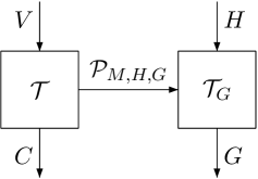
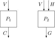
Figure 3: A TGE that interacts with a guided environment (left) and the corresponding distributed system architecture (right).

We examine whether viewing TGEs this way can help reduce SGE to known algorithms for the synthesis of distributed systems. We argue that the approach here, where we do not view $\hskip 1.5pt{\mathcal{T}}_{G}$ as a process in a distributed system, is preferable. In distributed-systems synthesis, we are given a specification $\varphi$ and an architecture describing the communication channels among processes. The goal is to design strategies for these processes so that their joint behavior satisfies $\varphi$. Synthesis of distributed systems is generally undecidable [9], primarily due to information forks – processes with incomparable information (e.g., when the environment sends assignments of disjoint sets of signals to two processes) [11]. The SGE setting corresponds to the architecture in Figure 3: Process $P_{1}$ is the TGE $\hskip 1.5pt{\mathcal{T}}$, which gets assignments to $V$ and generates assignments to $C$. Instead of designing $P_{1}$ to generate instructions for the environment, the synthesis algorithm also returns $P_{2}$, which instructs the environment on generating assignments to $G$. The process $P_{2}$ gets (in fact generates) assignments to both $V$ and $H$, eliminating information forks, making SGE solvable by solving distributed-system synthesis for this architecture. A solution in the TGE setting, that is composed of a TGE $\hskip 1.5pt{\mathcal{T}}$ and an environment transducer $\hskip 1.5pt{\mathcal{T}}_{G}$, induces a solution in the distributed setting: $P_{1}$ follows $\hskip 1.5pt{\mathcal{T}}$, and $P_{2}$ simulates the joint operation of $\hskip 1.5pt{\mathcal{T}}$ and $\hskip 1.5pt{\mathcal{T}}_{G}$, assigning values to $G$ as instructed by $\hskip 1.5pt{\mathcal{T}}$. Conversely, a TGE can encode through $\mathcal{P}_{M,H,G}$ the current assignment to $V$ together with a description of the structure of $P_{2}$, achieving the architecture in Figure 3 (right).

Using programs in $\mathcal{P}_{M,H,G}$ goes beyond sending $V$’s values, which are already known to the environment. Programs leverage the TGE’s computation, particularly its current state, to save resources and utilize less memory. Not using the communication channel between the TGE and the environment could result in a significant increase in the size of process $P_{2}$. For example, when $|M|=1$ (specifications where $G$’s assignment depends only on $V$’s history and $H$’s current assignment), the process $P_{2}$ is redundant. An explicit example is in Theorem VI.1, similar to the proof of Theorem III.3. As demonstrated in Section V, programs in $\mathcal{P}_{M,H,G}$ can be described symbolically. Formally, we have the following.

Theorem VI.1

For every $k\geq 1$, there exists a specification $\varphi_{k}$ over $V\cup H\cup G$, such that $\varphi_{k}$ is $(V,H,C,G)$-realizable by a TGE with a set of states and a memory set both of size $O(k)$, yet the size of $P_{2}$ in a distributed system that realizes $\varphi_{k}$ is at least $\Omega(k^{2})$.

Proof:

Let $V={\{v\}},H={\{h\}}$, and $G={\{d\}}$. Consider the specification $\varphi_{k}=Fd\leftrightarrow((F^{k}v)\wedge(F^{k}h))$, where the operator $F^{k}$ stands for “at least $k$ occurrences in the future” (see formal definition in Theorem III.3). Accordingly, the specification $\varphi_{k}$ requires that $d$ is eventually turned on iff both signals $v$ and $h$ are turned on at least $k$ times.

We prove that in the distributed setting, Process $P_{2}$ needs to implement two $k$-counters simultaneously, while a TGE may decompose the two counters between the system and the environment, implying the stated quadratic saving.

Note that the synthesis of $\varphi_{k}$ in a distributed setting forces the process $P_{2}$ to implement two $k$-counters, one for the number of times $v$ is on, and one for the number of times $h$ is on. Accordingly, $P_{2}$ needs at $\Omega(k^{2})$ states. On the other hand, synthesis of $\varphi_{k}$ by a TGE enables a decomposition of the two counters: The TGE $\hskip 1.5pt{\mathcal{T}}$ maintains a counter for $v$, and the environment transducer $\hskip 1.5pt{\mathcal{T}}_{G}$ needs to implement only a counter for $h$. Indeed, as long that the $v$ counter has a value below $k$, the TGE $\hskip 1.5pt{\mathcal{T}}$ sends to $\hskip 1.5pt{\mathcal{T}}_{G}$ a program that instruct it to assign $d$ with $\mathtt{F}$, and update its state according to $h$. Once the counter of $v$ reaches $k$, the TGE instructs $\hskip 1.5pt{\mathcal{T}}_{G}$ to turn $d$ on if its counter of $h$ reached $k$. Thus, there is a TGE with state space and memory set both linear in $k$. ∎

VII Discussion

We introduced synthesis with guided environments, where the system can utilize the knowledge and computational power of the environment. Straightforward directions for future research include extensions of the many settings in which synthesis has been studied to the “the guided paradigm”. Here we discuss two directions that are more related to the paradigm itself.

Dynamic hiding and guidance. In the setting studied here, the partition of $I$ and $O$ into visible, hidden, controlled, and guided signals is fixed throughout the computation. In some settings, these partitions may be dynamic. For example, when visibility depends on sensors that the system may activate and deactivate [13] or when signals are sometimes hidden in order to maintain the privacy of the system and the environment [16]. The decision which signals to hide in each round may depend on the system (e.g., when it instructs the environemnt which signals to hide in order to maintain its privacy), the environment (e.g., when it prefers not to share sensitive information), or an external authority (e.g., when signals become hidden due to actual invisibility). As for output signals, their guidance may depend on the history of the interaction (e.g., we may be able to assume amenability from the environment only after some password has been entered).

Bounded SGE. SGE involves a memory that can be used by the environment. As in the study of traditional bounded synthesis [26, 27], it is interesting to study SGE with given bounds on both the state spaces of the system and the environment. In addition to better modeling the setting, the bounds are used in order to improve the complexity of the algorithm, and they can also serve in heuristics, as in SAT-based algorithms for bounded synthesis [36]. In the setting of SGE, it is interesting to investigate the tradeoffs among the three involved bounds. It is easy to see that the two bounds that are related to the environment, namely the bound on its state space and the bound on the memory supervised by the system, are dual: an increase in the memory supervised by the system makes more specifications realizable, whereas an increase in the size of the state space of the environment makes fewer specifications realizable.

Another parameter that is interesting to bound is the number of different programs that a TGE may use, or the class of possible programs. In particular, restricting SGE to programs in which guided output signals can be assigned only the values of hidden signals or values stored in registers, will simplify an implementation of the algorithm. Likewise, the update of the memory during the interaction may be global and fixed throughout the computation.

References

- [1] R. Bloem, K. Chatterjee, and B. Jobstmann, “Graph games and reactive synthesis,” in Handbook of Model Checking. Springer, 2018, pp. 921–962.
- [2] A. Pnueli and R. Rosner, “On the synthesis of a reactive module,” in Proc. 16th ACM Symp. on Principles of Programming Languages, 1989, pp. 179–190.
- [3] R. Bloem, R. Ehlers, and R. Könighofer, “Cooperative reactive synthesis,” in 13th Int. Symp. on Automated Technology for Verification and Analysis, 2015, pp. 394–410.
- [4] A. Anand, K. Mallik, S. Nayak, and A.-K. Schmuck, “Computing adequately permissive assumptions for synthesis,” in Proc. 29th Int. Conf. on Tools and Algorithms for the Construction and Analysis of Systems. Springer, 2023, pp. 211–228.
- [5] J. Reif, “The complexity of two-player games of incomplete information,” Journal of Computer and Systems Science, vol. 29, pp. 274–301, 1984.
- [6] O. Kupferman and M. Vardi, “Synthesis with incomplete information,” in Advances in Temporal Logic. Kluwer Academic Publishers, 2000, pp. 109–127.
- [7] K. Chatterjee, L. Doyen, T. Henzinger, and J.-F. Raskin, “Algorithms for omega-regular games with imperfect information,” Logical Methods in Computer Science, vol. 3, no. 3, 2007.
- [8] R. Rosner, “Modular synthesis of reactive systems,” Ph.D. dissertation, Weizmann Institute of Science, 1992.
- [9] A. Pnueli and R. Rosner, “Distributed reactive systems are hard to synthesize,” in Proc. 31st IEEE Symp. on Foundations of Computer Science, 1990, pp. 746–757.
- [10] O. Kupferman and M. Vardi, “Synthesizing distributed systems,” in Proc. 16th ACM/IEEE Symp. on Logic in Computer Science, 2001, pp. 389–398.
- [11] S. Schewe, “Synthesis of distributed systems,” Ph.D. dissertation, Saarland University, Saarbrücken, Germany, 2008.
- [12] K. Chatterjee, R. Majumdar, and T. A. Henzinger, “Controller synthesis with budget constraints,” in Proc 11th International Workshop on Hybrid Systems: Computation and Control, ser. Lecture Notes in Computer Science, vol. 4981. Springer, 2008, pp. 72–86.
- [13] S. Almagor, D. Kuperberg, and O. Kupferman, “Sensing as a complexity measure,” Int. J. Found. Comput. Sci., vol. 30, no. 6-7, pp. 831–873, 2019.
- [14] B. Finkbeiner, N. Metzger, and Y. Moses, “Information flow guided synthesis with unbounded communication,” in Proc. 36th Int. Conf. on Computer Aided Verification. Springer Nature Switzerland, 2024, pp. 64–86.
- [15] Y. Wu, V. Raman, B. Rawlings, S. Lafortune, and S. Seshia, “Synthesis of obfuscation policies to ensure privacy and utility,” Journal of Automated Reasoning, vol. 60, no. 1, pp. 107–131, 2018.
- [16] O. Kupferman and O. Leshkowitz, “Synthesis of privacy-preserving systems,” in Proc. 42nd Conf. on Foundations of Software Technology and Theoretical Computer Science, ser. Leibniz International Proceedings in Informatics (LIPIcs), vol. 250, 2022, pp. 42:1–42:23.
- [17] R. Alur, T. Henzinger, and O. Kupferman, “Alternating-time temporal logic,” Journal of the ACM, vol. 49, no. 5, pp. 672–713, 2002.
- [18] R. Berthon, B. Maubert, A. Murano, S. Rubin, and M. Vardi, “Strategy logic with imperfect information,” in Proc. 32nd ACM/IEEE Symp. on Logic in Computer Science, 2017, pp. 1–12.
- [19] J. Gutierrez, G. Perelli, and M. J. Wooldridge, “Imperfect information in reactive modules games,” Inf. Comput., vol. 261, pp. 650–675, 2018.
- [20] A. Krausz and U. Rieder, “Markov games with incomplete information,” Mathematical Methods of Operations Research, vol. 46, pp. 263–279, 1997.
- [21] K. Chatterjee, L. Doyen, S. Nain, and M. Vardi, “The complexity of partial-observation stochastic parity games with finite-memory strategies,” in Proc. 17th Int. Conf. on Foundations of Software Science and Computation Structures, ser. Lecture Notes in Computer Science, vol. 8412. Springer, 2014, pp. 242–257.
- [22] R. Kumar and M. Shayman, “Formulae relating controllability, observability, and co-observability,” Autom., vol. 34, no. 2, pp. 211–215, 1998.
- [23] G. De Giacomo and M. Y. Vardi, “Ltlf and ldlf synthesis under partial observability,” in Proc. 25th Int’l Joint Conf. on Artificial Intelligence. IJCAI/AAAI Press, 2016, pp. 1044–1050.
- [24] P. Bouyer, N. Markey, and S. Vester, “Nash equilibria in symmetric graph games with partial observation,” Information and Computation, vol. 254, pp. 238–258, 2017.
- [25] E. Filiot, R. Gentilini, and J.-F. Raskin, “Rational synthesis under imperfect information,” in Proc. 33rd ACM/IEEE Symp. on Logic in Computer Science. ACM, 2018, pp. 422–431.
- [26] S. Schewe and B. Finkbeiner, “Bounded synthesis,” in 5th Int. Symp. on Automated Technology for Verification and Analysis, ser. Lecture Notes in Computer Science, vol. 4762. Springer, 2007, pp. 474–488.
- [27] O. Kupferman, Y. Lustig, M. Vardi, and M. Yannakakis, “Temporal synthesis for bounded systems and environments,” in Proc. 28th Symp. on Theoretical Aspects of Computer Science, 2011, pp. 615–626.
- [28] A. Pnueli, “The temporal semantics of concurrent programs,” Theoretical Computer Science, vol. 13, pp. 45–60, 1981.
- [29] M. Vardi and P. Wolper, “Reasoning about infinite computations,” Information and Computation, vol. 115, no. 1, pp. 1–37, 1994.
- [30] O. Kupferman and M. Vardi, “Safraless decision procedures,” in Proc. 46th IEEE Symp. on Foundations of Computer Science, 2005, pp. 531–540.
- [31] Y. Gurevich and L. Harrington, “Trees, automata, and games,” in Proc. 14th ACM Symp. on Theory of Computing. ACM Press, 1982, pp. 60–65.
- [32] M. Vardi and P. Wolper, “Automata-theoretic techniques for modal logics of programs,” Journal of Computer and Systems Science, vol. 32, no. 2, pp. 182–221, 1986.
- [33] S. Safra, “On the complexity of -automata,” in Proc. 29th IEEE Symp. on Foundations of Computer Science, 1988, pp. 319–327.
- [34] J. Esparza, J. Kretínský, and S. Sickert, “A unified translation of linear temporal logic to -automata,” J. ACM, vol. 67, no. 6, pp. 33:1–33:61, 2020.
- [35] S. Akshay, E. Basa, S. Chakraborty, and D. Fried, “On dependent variables in reactive synthesis,” in Proc. 30th Int. Conf. on Tools and Algorithms for the Construction and Analysis of Systems. Springer Nature Switzerland, 2024, pp. 123–143.
- [36] R. Ehlers, “Symbolic bounded synthesis,” in Proc. 22nd Int. Conf. on Computer Aided Verification, ser. Lecture Notes in Computer Science, vol. 6174. Springer, 2010, pp. 365–379.