Effective conductivity of conduit networks with random conductivities

Abstract

The effective conductivity ($T^{eff}$) of 2D and 3D Random Resistor Networks (RRNs) with random edge conductivity is studied. The combined influence of geometrical disorder, which controls the overall connectivity of the medium and leads to percolation effects, and conductivity randomness is investigated. A formula incorporating connectivity aspects and second-order averaging methods, widely used in the stochastic hydrology community, is derived and extrapolated to higher orders using a power averaging formula based on a mean-field argument. This approach highlights the role of the so-called resistance distance introduced by graph theorists. Simulations are performed on various RRN geometries constructed from 2D and 3D bond-percolation lattices. The results confirm the robustness of the power averaging technique and the relevance of the mean-field assumption.

I Introduction

Modeling transport in strongly heterogeneous materials is a generic issue that was addressed long ago in the 19th century[1], and later enriched[2, 3, 4, 5] among others in their respective research areas. Applications range from modeling mechanical properties of composite media, heat transfers, electrical currents, to momentum transfers in porous media at different scales. Restricting ourselves mainly to the former area, many theoretical approaches have been proposed by theoretical hydrologists [6, 7, 8, 9, 10], by mathematicians [11, 12] and physicists [13, 14, 15, 16, 17, 18, 19, 20, 21, 19, 22, 23, 24], reflecting the diversity of backgrounds such as volume averaging, homogenization, multiple-scale expansion methods, and stochastic perturbation theory.
In order to model flow in porous network models or fractured media, that correspond to extremely contrasted local flow properties, the framework of percolation theory is more adapted [25, 26, 27, 28, 29, 30, 31, 32]. Karstic aquifers are even more extreme and complex underground multiscale structures, that include caves, sinkholes, and fracture networks. Modeling groundwater motion within such systems is a major societal issue in the context of overall climate change. The increasing occurrence of extreme events (droughts, floods) justifies building predictive models that remain robust even when forced by extreme data [33, 34, 35]. This requires constructing a model that captures the main subsurface processes involved in such systems while representing their internal geometrical complexity as accurately as possible. It is appealing to adapt a model based on a network of conduits that can be characterized through direct exploration, staying close to the so-called distributed model approach. It differs from reservoir models and neural networks [36, 37] the aim of which is to relate input data (recharge) to rates at springs without refereeing to an explicit knowledge of the subsurface. The model is calibrated through data history, so working well in generic recharge conditions, but accuracy may be lost if extreme forcing conditions are not present in the calibration data basis.

A natural representation of these structures can be achieved using a graph-theoretical framework as proposed by [38] and references therein, which captures the interconnections of different elements. To describe fluid flow in these networks, assuming they are saturated and within the linear (Darcean) assumptions, they can be modeled as a Random Resistor Network (RRN). These RRNs can be mathematically described using a graph or a lattice where each connection, or edge, between vertices $i$ and $j$ (points in the lattice) is assigned an element that can be assimilated to a resistor with a conductivity $T_{ij}$ that does not depend on the local potential difference, up to a first approximation.

In this study, we explore the interplay between the geometry of the underlying network and the conductivity distribution, and how both randomness influence the effective conductivity of RRNs. Before using more formal definitions, the effective conductivity can be defined as the scaling factor that matches the response of the heterogeneous network to that of its “average” counterpart under a given large-scale forcing. The imposed forcing may correspond to the usual forced flow in a given direction, as provided by homogenization and fluxes averaging theories. It can also correspond to forcing boundary conditions such as recharge areas, catchments, etc. This allows the definition of a so-called effective conductivity that summarizes the overall behavior of the RRN and may help in devising a reduced-order model described by less degrees of freedom. The situation may be more subtle when starting from a purely network approach that does not refer to any underlying Euclidean metric, precluding the idea of an imposed large-scale head gradient. The corresponding fluxes and potential drops are studied to highlight localization phenomena (channeling) where a small subset of the network controls the overall flow properties, carrying most of the flow.

As stated above, two kinds of disorder may coexist: a geometrical disorder, encapsulated in the so-called adjacency matrix of the graph that summarizes the connections between vertices, and a conductivity disorder, which describes the various conduit conductivity that may be encountered. In the porous network or karst case, these values depend on network sub-scale details, the precise pore or conduit geometry [39]. As a first approximation, these can be considered positive random variables, assumed to be independent on the network geometry.

Considering a uniform conductivity distribution with a value $T_{0}$, the dominant descriptor is an order-parameter $p$ that controls the overall connectivity of the network. It is typically the proportion of active bonds (or edge in a graph-theoretic language). The framework offered by percolation theory is well-known among the physics and hydrology communities. The critical behavior and localization phenomena leading to critical path analysis can be found in review papers and textbooks [26, 27, 40, 30]. Investigations in this area have been carried out by researchers interested in flow through Discrete Fracture Networks (DFN), such as [41, 42, 43]. This field has long incorporated graph theory to model flow in DFNs.

On the other hand, if the geometric disorder is low and the randomness of the conductivity values dominates, it is common practice, particularly within the geoscience community, to use upscaled numerical models. The discretized flow equations are solved using a simulator that uses a coarse grid that smooths the fine scale details of the input conductivity map. In such approaches, it is customary to determine coarse grid properties from their corresponding high resolution counterpart provided by geologists [44] using simplified approaches. Many techniques exist, as presented in review papers on the subject already cited above. Among these techniques we focus on power averaging [4, 45, 46, 47]. It allows quick characterization of the effective conductivity of heterogeneous formations by spatially averaging the conductivity field over a volume that may correspond to any coarse grid block employed by flow simulators, its expression is given by:

$$K^{eff} = \langle K^{\omega}\rangle^{\frac{1}{\omega}}$$ (1)

Here, $\omega$ is an exponent such that $-1\leq\omega\leq 1$, which depends on the dimension $D=1,2,3$ of the space and on the spatial arrangement of the conductivity. Upon computing the limit, the value $\omega=0$ corresponds to the geometric mean $K_{g}=\exp(\langle\log(K)\rangle)$. This provides a practical way to approximate conductivity upscaling, even though its theoretical foundations are mainly limited to specific models and conditions. Numerical tests show that power averaging is quite robust, even for large value of the log-conductivity variance [47, 24, 32].
Fewer studies exist where both disorders are present [48, 49]. Such combined models are more realistic since most natural conductive systems may be well-connected but not necessarily close to any percolation threshold, implying to be studied using more case by case basis because the so-called universal results of percolation theory may be lost. In many cases, local conductivity variability may compete with connectivity effect on large-scale flow behavior. In situations where it dominates, many studies and classical textbooks address this topic in the hydrology or oil and gas literature [4, 10, 50, 51, 52, 24]. The basic concepts involve averaging and upscaling models that provides solutions to following issue: how to propagate heterogeneity from the fine scale to the overall scale of the system, which is more relevant for applications. In these fields, simulations are carried out using flow simulators that solve discrete forms of the conservation equations. Great care is taken to account for boundary conditions at aquifer boundaries or at wells, if present. In this context, current practice in upscaling mainly involves grid coarsening and pragmatic solutions to following issue: how to coarsen the mesh while accounting for as many sub-coarse grid details as possible, which can drastically change the overall flow behavior.

In present paper that interaction between geometry and heterogeneity is studied considering model RRN’s described by a proportion of active edges controlling the overall connectivity, and an heterogeneity described by means of a conductivity distribution. The former will be carried out considering model networks constructed from 2D or 3D lattices having various connectivity descriptor (typically a proportion $p$ of active edges), using conductivity distributions following a log-normal law.
The paper is organized as follows. In next Sec. II.1, the model and notations are introduced. Then in Sec. II.2, we develop a perturbation theory with respect to the conductivity fluctuation variance, starting from an arbitrary average connected network. Percolation theory overall framework is not presented, we refer to classical textbooks. That allows to set-up some connections between percolation and perturbation theory. The basic approach is to average over the conductivity disorder at fixed network geometry. The aim is to answer the following question: is it possible to replace RRN’s with random conductivities by another so-called equivalent RRN characterized by a so called equivalent conductivity that may be computed from the local conductivity distribution using e.g. a power averaging formula. Such an extrapolation of second-order perturbation results may be justified using a mean-field argument presented in Appendix A. Another approach in which an overall effective conductivity is determined such that the response of the full RRN to an overall forcing are similar: that is closer to standard definitions of effective parameters used by hydrologists. As will be shown in Sec. II.3, it is possible to achieve this up to the second order while retaining the same underlying network of active edges. A similar mean-field argument presented in Appendix B allows to present the result under a more robust power averaging form valid for higher variances. That allows to discard the conductivity disorder, focusing on overall connectivity issues. Upscaling methods where it is looked for a sparsified network involving less degrees of freedom are not addressed in present paper and will be the topic of another study. In next Sec. III, the numerical methodology is presented, including RRN generation procedures that were carried out. Then numerical results are treated within the proposed theoretical framework in Secs. II.4 and IV. It is shown that replacing the RRN with random conductivities by an “homogeneous” one with rescaled conductivities by means of a power law formula can be efficient, even for quite large log conductivity variance for which perturbation theory results breakdown.

II Theoretical considerations

II.1 Model and notations

We consider a RRN represented by a connected undirected graph of N vertices $G=(V,E)$. To each edge $<i,j>\in E$ connecting vertices $i$ and $j$, a conductivity $T_{ij}=T_{ji}\neq 0$ is selected randomly on a distribution of positive real number of pdf $p_{ij}$. They are assumed to be independent on each other. The number of edges is $N_{E}$.
We consider the set of potentials $\mathbf{P}=(P_{1},...,P_{N})^{\top}$ solution of the linear system corresponding to solving Kirchoff’s laws:

$$\forall i\sum_{j\in<i>}T_{ij}(P_{j}-P_{i})=Q_{i}$$ (2)

$$\sum_{i}P_{i}=0$$ (3)

The last equation allows to get a well-defined set of equations, as potentials are defined up to an arbitrary additive constant.

Similarly, the source terms $Q_{i}$ are such that $\sum_{i}Q_{j}=0$. The set of labels $<i>$ denotes the set of vertices connected to vertex $i$ by one edge. As the graph is connected, the normalization conditions for both $\mathbf{P}$ and $\mathbf{Q}$ give a well-defined unique solution. For short, this linear system may be written $\mathbf{L\cdot P=Q}$, in which $\mathbf{L}$ summarizes the corresponding matrix of the linear system Eqs. 2 and  3.

II.2 Averaging procedure

In most practical cases, we are interested by the average solution $\bar{P}_{i}=\langle P_{i}\rangle$, which unfortunately is not the solution of the average set of equations. The average $\langle\dots\rangle$ is to be evaluated over all the set of $T_{ij}$’s weighted by their respective pdf’s. More specifically, we look for an effective equation relating $\bar{P}_{i}$ to $\mathbf{Q}$. So, we seek whether $\bar{P}_{i}$ satisfies an effective set of averaged equations of the form:

$$\forall i\sum_{j}T^{eff}_{ij}(\bar{P}_{j}-\bar{P}_{i})=Q_{i}$$ (4)

$$\sum_{i}\bar{P}_{i}=0$$ (5)

Note that in that equation, it is not assumed that summations over $j$ are restricted to the initial set of vertices $<i>$ incident to $i$ in the starting point problem. In addition, it is implicitly assumed that the average potentials follow a Kirchoff’s like set of equations, that will be justified right now. In formal terms, we are investigating the following matrix $\mathbf{L}^{eff}=\langle\mathbf{L}^{-1}\rangle^{-1}$. Although at first sight $\mathbf{L}$ is not invertible, the condition 5 combined with the no net source term condition $\sum_{i}Q_{j}=0$ gives sense to the inverse in the relevant subspace. It can be observed that $\mathbf{L}^{eff}$ is obviously symmetric, being the invert of a symmetric matrix.
In order to check that $\mathbf{L}^{eff}$ possesses the structure of a Laplacian matrix, it is useful to decompose $\mathbf{L}$ under the form $\mathbf{L}=\mathbf{L_{0}}+\delta\mathbf{L}$. The matrix $\mathbf{L_{0}}$ is determined using average conductivities $\langle T_{ij}\rangle$ and $\delta\mathbf{L}$ corresponds thus to the fluctuating part of the Laplace operator written using $\delta T_{ij}$ of null average. Thus, $\mathbf{L_{0}}$ corresponds to the average set of equations.
Writing $(\mathbf{L_{0}}+\delta\mathbf{L})^{-1}=\mathbf{L_{0}}^{-1}(\mathbf{1}+\delta\mathbf{L}\mathbf{L_{0}}^{-1})^{-1}$, one obtain: $\mathbf{L}^{eff}=\langle(\mathbf{1}+\delta\mathbf{L}\mathbf{L_{0}}^{-1})^{-1}\rangle^{-1}\mathbf{L_{0}}$. Assuming that $\mathbf{M}=\langle(\mathbf{1}+\delta\mathbf{L}\mathbf{L_{0}}^{-1})^{-1}\rangle^{-1}$ is a well-defined matrix. $\mathbf{L_{0}}$ is a Laplacian matrix such that $\sum_{j}L_{i,j}=0$, so a similar property may be derived for $\mathbf{L}^{eff}=\mathbf{M}.\mathbf{L_{0}}$ because $\mathbf{L}^{eff}_{ij}=\sum_{k}M_{ik}L_{kj}$, so $\sum_{j}\mathbf{L}^{eff}_{ij}=\sum_{k}\sum_{j}M_{ik}L_{kj}=0$. As $\mathbf{L}^{eff}$ is symmetric, gathering these equalities, that confirms that $\mathbf{L}^{eff}$ has the structure of a Laplacian matrix leading to an effective set of equations sharing the form 5. Notice that this result is quite general and does not rely on a specific conductivity distributions nor on any order of a perturbation expansion.

That procedure corresponds physically to most averaging techniques employed in that class of issues, in which the source terms such as boundary conditions, imposed potentials are known on few points, and internal degrees of freedom of the bulk that follow conservation equations are to be eliminated from the problem, resulting in solving local equations. In analogy with continuous Laplace equations averaging [16], it can be anticipated that $\mathbf{L}$ being a sparse matrix having ($N\leq N_{non\ zero\ entries}\ll N^{2}$ non zero elements), $\langle\mathbf{L}^{-1}\rangle$, can be expected to be a full matrix of $N^{2}$ elements (reflecting the long-ranged character of Laplace equation Green’s function). But it can also be anticipated that $\langle\mathbf{L}^{-1}\rangle^{-1}$ may be sparse, or have exponentially small matrix elements far from the diagonal (although in the context of graphs, a more precise meaning should be given to that statement in terms on an intrinsic distance on the graph) such as the chemical distance between nodes. That may be justified studying carefully the matrix $\mathbf{M}=\langle(\mathbf{1}+\delta\mathbf{L}\mathbf{L_{0}}^{-1})^{-1}\rangle^{-1}$. Extrapolating results obtained in the continuous case context [16], it can be observed that $\mathbf{M}$ may be similar to the inverse Fourier transform of $\dfrac{1}{1+(qa)^{2}+\cdots}$ in which … represent higher powers of $q$. Coming back to real domain, that provides an operator having exponentially decreasing elements in the real domain. Having a direct and rigorous derivation in the graph theoretic context would be useful.
In the case of the continuous Laplace equation, it can be shown [16] that for an infinite system, such a definition coincides with the usual, more intuitive definitions involving estimations of the mean flux as a response to an imposed head gradient. Following that procedure, effective conductivities $T_{ij}^{eff}$ are to be estimated from the input data, which requires the use of perturbation expansion methods to obtain explicit results.

II.3 Second order perturbation expansion results

In order to set-up a perturbation expansion, we write $(\mathbf{L_{0}}+\delta\mathbf{L})^{-1}=\mathbf{L_{0}}^{-1}(\mathbf{1}+\delta\mathbf{L}\mathbf{L_{0}}^{-1})^{-1}$, then the second factor may be expanded in Neumann series, that is equivalent to solve the equations by an iterative geometric sequence. After some manipulations we obtain:

$$\langle\mathbf{L}^{-1}\rangle^{-1}=[\mathbf{L_{0}}^{-1}\langle(\mathbf{1}+\delta\mathbf{L}\mathbf{L_{0}}^{-1})^{-1}\rangle]^{-1}$$

$$=\mathbf{L_{0}}[\mathbf{L_{0}}+\sum_{n=1}^{\infty}(-1)^{n}\langle(\delta\mathbf{L}\mathbf{L_{0}}^{-1})^{n}\rangle\mathbf{L_{0}}]^{-1}\mathbf{L_{0}}$$ (6)

The averaging process can be carried out using that series expansion, but due to the inversion of the series of matrices between brackets in equation 6, computation of high order terms becomes quickly cumbersome at high orders. In the continuous case, considering a D-dimensional random conductivity problem, some general results allowing to get an alternative form of a series expansion of $\langle\mathbf{L}^{-1}\rangle^{-1}$ in terms of a series involving so-called 1P irreducible Feynman diagrams containing correlation functions of conductivity fluctuations of increasing order can be obtained [16]. That summation by-passes the inversion of the sum of series of matrices between brackets in equation 6. That confirms the fact that $\langle\mathbf{L}^{-1}\rangle^{-1}$ shares essentially the same structure than the original average Laplace operator $L_{0}$.
We were not able to derive such a summation formula in present discrete case, so right now the analysis is limited to the second order expansion that is given by:

$$\langle\mathbf{L}^{-1}\rangle^{-1}=[\mathbf{L_{0}}^{-1}\langle(\mathbf{1}+\delta\mathbf{L}\mathbf{L_{0}}^{-1})^{-1}\rangle]^{-1}$$

$$\simeq\mathbf{L_{0}}[\mathbf{L_{0}}+\langle(\delta\mathbf{L}\mathbf{L_{0}}^{-1})^{2}\rangle\mathbf{L_{0}}]^{-1}\mathbf{L_{0}}$$

$$=\mathbf{L_{0}}-\langle\delta\mathbf{L}\mathbf{L_{0}}^{-1}\delta\mathbf{L}\rangle$$ (7)

$$=\mathbf{L_{0}}-\mathbf{\Sigma}$$ (8)

The matrix $\mathbf{\Sigma}\simeq\langle\delta\mathbf{L}\mathbf{L_{0}}^{-1}\delta\mathbf{L}\rangle$ is called the self-energy in condensed matter physics [16].

The net second order result can be evaluated, computing the product $\mathbf{\Sigma}.\mathbf{P}$:

Using the equality: $\langle\delta T_{ik}\delta T_{lj}\rangle=\sigma_{ik}^{2}[\delta_{il}\delta_{kj}+\delta_{ij}\delta_{kl}]$, one gets:

$$(\mathbf{\Sigma}\cdot\mathbf{P})_{i}=\sum_{j\in<i>}\sigma_{ij}^{2}[{L_{0}}^{-1}_{ij}+{L_{0}}^{-1}_{ji}-{L_{0}}^{-1}_{ii}-{L_{0}}^{-1}_{jj}](P_{j}-P{{}_{i}})$$ (9)

It appears that up at second order, the matrix $\langle\mathbf{L}^{-1}\rangle^{-1}$ couples the same vertices than the average input $\mathbf{{L}_{0}}$, so the associated connectivity matrix is the equal to the initial one up to that order. The symmetry of $\mathbf{\Sigma}$ appears clearly as it should. The quantity $R_{ij}=[{L_{0}}^{-1}_{ij}+{L_{0}}^{-1}_{ji}-{L_{0}}^{-1}_{ii}-{L_{0}}^{-1}_{jj}]$ has a sound physical interpretation, it corresponds to the potential difference between vertices i and j computed using the average RRN given that a unit strength source/sink dipole is located on vertices i and j. In graph theory it corresponds to the so-called resistance distance introduced by [53], a major topic in modern graph theory context [54]. The edge effective conductivity $T_{ij}^{eff}$ can be estimated up to second-order from that formula. In order to get a more robust estimator capturing higher variance, a mean-field theory is presented in Appendix A that allows to justifies the power-average extrapolation Eq. 1 sharing the same second order expansion.

II.4 Results for structured RRN, percolation networks

The preceding calculations can be specialized for D dimensional structured networks, such as those resulting from the discretization of a Laplace equation in a D dimensional space using finite differences with a 2D+1 stencil. In such a case, the corresponding RRN equations read:

$$\sum_{\epsilon_{i{{}_{k}=}}\pm 1}T_{i_{1},\dots i_{D};i_{1}+\epsilon_{i_{1}},\dots i_{D}+\epsilon_{i_{D}}}(P_{i_{1}+\epsilon_{i_{1}},\dots i_{D}+\epsilon_{i_{D}}}-P_{i_{1},\dots i_{D}})=Q_{i_{1},\dots i_{D}}$$

The average matrix $\mathbf{L_{0}}$ is symmetric, it has 2D+1 diagonals, a generic line having the form

$$\langle T\rangle(0\cdots 1,1,..,-2D,1,1,1,0\cdots 0)$$

with $2D\times$ unit values off diagonal, and -2D on the diagonal. Assuming a uniform conductivity variance $\sigma^{2}$, one obtains in the limit of a large network, Appendix B:

$$(\mathbf{\Sigma}\cdot\mathbf{P})_{\bf i}=\sum_{{\bf j}\in<{\bf i}>}\frac{\sigma^{2}}{\langle T\rangle D}(P_{{\bf j}}-P{{}_{\bf i}})$$ (10)

Here ${\bf i}$ (resp. ${\bf j}$) denotes the multi-index ${\bf i}=(i_{1},\dots i_{D})$ (resp. ${\bf j}=(j_{1},\dots j_{D}))$. For D=1, considering a path graph such as those considered in Appendix C, the formula is exact without any large N assumption. In other cases, assuming a large RRN, and that the statistical properties of $T_{ij}$ do not depend on the edge $ij$, it can be shown that up to second order, the system behaves as an effective RRN with conductivities:

$$T^{eff}_{\bf ij} = \langle T_{\bf ij}\rangle\left(1-\frac{1}{D}\frac{\sigma^{2}}{\langle T_{\bf ij}\rangle^{2}}+\cdots\right)$$ (11)

$$\simeq \langle T_{g\bf ij}\rangle exp(1/2-1/D)\sigma_{\log T}^{2}=\langle T_{\bf ij}^{(1-2/D)}\rangle^{\frac{1}{(1-2/D)}}.$$

Here, $T_{g\bf ij}=exp\langle\log T_{\bf ij}\rangle$ and $\sigma_{\log T}^{2}$ are respectively the geometric average of the edge ij conductivity and the associated log-conductivity variance. A mean-field argument allowing to justify that extrapolation is given in A. We used textbooks formula for estimating power averages of log-normal distributions. This last form that shares the same second order expansion is a result known under the name of Landau-Lifshitz-Matheron conjecture [2, 4, 15] that was derived in the context of continuous Laplace problems in heterogeneous media. That conjecture is exact at all orders for D=1, in which a complete analytical solution is available (Appendix C). In 2D, it is exact for specific log-normal distribution or close to percolation thresholds [4, 55]. In the 3D continuous case, it was shown to be inexact using 6 th order expansion [56, 9, 22], although it was observed to be very accurate in the numerical practice [47, 57, 58].
In cases where connections are kept with probability $p$ close to 1 (full network), an estimation of $\omega$ is given by a quite simple formula (derivation in Appendix B).

$$\omega\approx 1-2*\frac{N_{\text{p}}}{N_{\text{E}}}$$ (12)

Here, $N_{\text{E}}$ represents the number of active edges, the set of edges that are available to flow. $N_{\text{p}}$ denotes the number of vertices connected to these edges (active vertices). The equation can be expressed in terms of $k$, the average degree of a node in the graph, where $k=\frac{2N_{\text{E}}}{N_{\text{p}}}$, thus $\omega=1-\frac{4}{k}$. This expression satisfies two conditions: (1) As $p\to 1$, it yields the value of $\omega$ known for 2D and 3D full networks with a lognormal conductivity distribution, where $\omega=0$ for 2D and $\omega=\frac{1}{3}$ for 3D networks; and (2), when $\frac{N_{\text{p}}}{N_{\text{E}}}=1$, it results in $\omega=-1$, the exact value for 1D networks (corresponding to the harmonic mean). A 1D backbone network may behave as a 1D network when $p=p_{c}$.

III Numerical Methodology

This section details the methodology used to generate Random Resistor Networks (RRNs) for investigating the impact of conductivity and geometric disorders on the effective conductivity, $T^{eff}$. In these networks, geometric disorder is introduced through the random removal of edges, while conductivity disorder is implemented by varying the conductivity values assigned to the edges.

III.1 Generation of RRNs

III.1.1 Generation of 2D and 3D lattice RRN with r=1

Nodes are placed on a regular square (2D) or cubic (3D) grid. In this configuration, each node is connected only to its immediate orthogonal neighbors (excluding diagonal connections) to emulate a lattice structure commonly explored in classical percolation theory [55]. This connectivity setup, defined by a radius r$=1$, ensures that nodes interact only with their nearest orthogonal neighbors. Geometry is varied by selectively removing edges, effectively setting their conductivity to zero. The connectivity proportion $p$ directly dictates the probability of an edge being retained, simulating different scenarios from sparse to fully connected networks as $p$ varies from the percolation threshold $p_{c}$ to 1. On the other hand, conductivities are assigned independently from a lognormal distribution with a unitary geometric mean, reflecting the natural variability of conduit sizes [39]. The variance of the logarithm of this distribution, $\sigma^{2}_{\log T}$, controls the heterogeneity within the network. Examples of these network configurations can be seen in Fig. 1, which illustrates structured networks at the critical degree ($p=p_{c}$) near the percolation threshold.

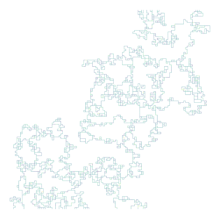
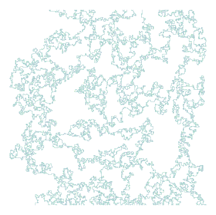
Figure 1: Networks at the critical degree ($p\approx p_{c}$), with 2D networks ($128\times 128$ nodes) on the left and 3D networks ($48\times 48\times 48$ nodes) on the right. Edge colors represent conductivity values.

III.1.2 Structured RRNs with $r>1$

For networks where the connectivity radius $r$ extends beyond the immediate neighbors, we simulate a transition from local to global connectivity. The radius $r$ serves as a scaling parameter that, along with $p$, adjusts connectivity and shapes the network’s structure. This scaling allows for the exploration of network behaviors across a continuum of connectivity regimes.

The proportion $p$ is defined as $p=k/k_{r}$, where $k$ represents the average degree of connectivity after edge removal, and $k_{r}$ represents the average degree of a node in a network where all nodes within a distance $r$ from each other are connected. This degree depends on the radius $r$, as a larger radius increases the number of neighboring nodes that can be connected to each other. Similar strategies are employed to study ad hoc wireless networks under varying parameters of radius and connectivity [59]. Examples of these network configurations are visually represented in Fig. 2, which displays structured networks at connectivity near the critical degree ($k\approx k_{c}$) for a radius of $r=5$.

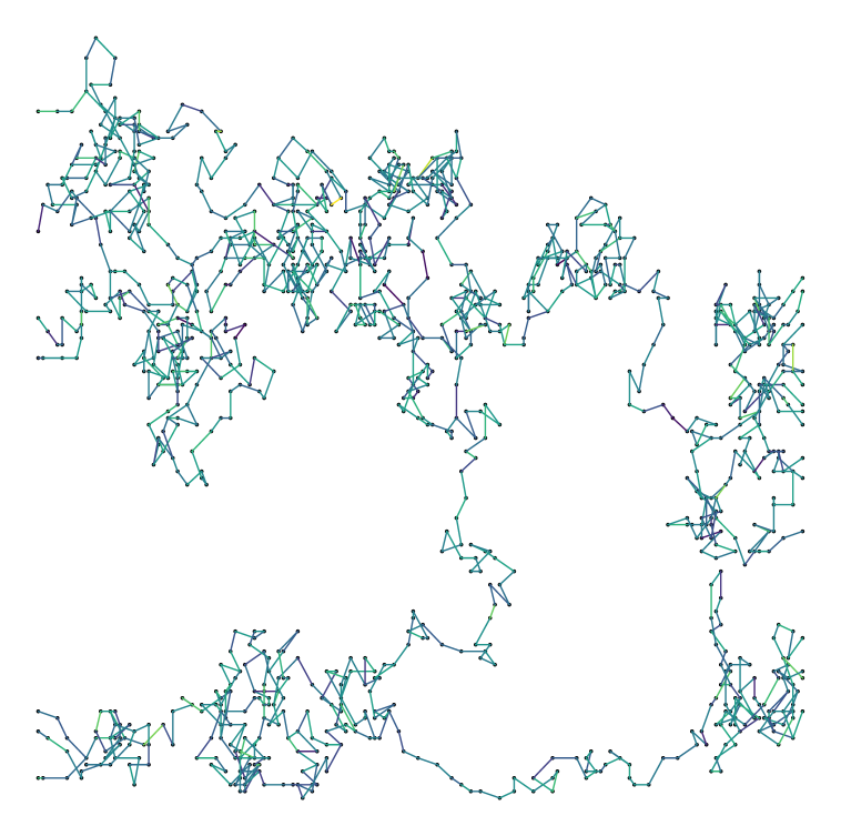
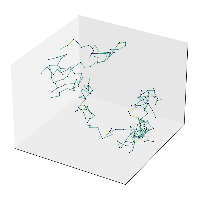
Figure 2: Examples of structured networks at critical connectivity ($p\approx p_{c}$): on the left, a 2D network with $200\times 200$ nodes, and on the right, a 3D network with $48\times 48\times 48$ nodes. These networks incorporate a connectivity radius $r=5$, that extends beyond nearest neighbors, altering the overall connectivity. Edge colors represent conductivity values.

III.2 Simulation of Flow and postprocessing of the solution

The potential at each node is computed by solving Kirchhoff’s laws, as shown in Eq. 3, with a potential difference $\Delta P$ applied between the nodes in the inlet and the nodes in the outlet. In structured networks, where nodes are systematically arranged on a regular grid, the inlet is designated on one face of the domain, and the outlet is positioned on the opposite face.

The distance $L$ between the inlet and outlet is defined as the number of edges $N_{x}-1$. The cross-sectional area $A$, perpendicular to the flow direction, is calculated as $(N_{y}-1)\times(N_{z}-1)$. Here, $N_{x}$, $N_{y}$, and $N_{z}$ represent the original number of nodes along each dimension before any removal of edges.

Effective conductivity, $T^{eff}$, encapsulates the hydraulic response of the network under a given large-scale forcing, and is computed by:

$$T^{eff}=\frac{Q_{T}}{\Delta P}\frac{L}{A}$$ (13)

where $Q_{T}$ denotes the total flow.

To optimize the simulation process and minimize computational costs, a network pruning process is implemented prior to conducting flow simulations is applied before simulations begin [60]. This process removes nodes of degree zero and one, which do not contribute to flow, and retains only nodes within the largest cluster. Following the pruning process, the linear system is solved to determine the potential at each node, leading to the computation of flow at each edge. This solution enables the computation of the number of active edges $N_{\text{E}}$ and active nodes $N_{\text{p}}$, and the calculation of the parameter $\omega$ using Eq. 12.

In order to get a better understanding of the influence of both disorders about the effective large scale conductivity, the following procedure was employed. The main idea is to account for the conductivity disorder by modifying the power law averaging method.

Firstly, for a lognormal distribution of conductivities, the power average of the input distribution is given by:

$$\langle T^{\omega}\rangle^{\frac{1}{\omega}}=T_{g}\exp{\left(\omega\frac{\sigma_{\log T}^{2}}{2}\right)}$$ (14)

Here, $T_{g}$ represents the geometric mean of the lognormal distribution, and $\sigma_{\log T}^{2}$ is the variance of its logarithm. For a specified set of parameters $\sigma_{\log T}^{2},p$, an effective conductivity $T^{eff}(\sigma_{\log T}^{2},p)$ can be calculated by solving the Kirchhoff equations. In the case of a fully connected RRN, the exponent $\omega$ is determined by matching this formula with the numerically obtained $T^{eff}$. This involves replacing the conductivity of each edge with a uniform value given by $T^{eff}$, resulting in an equivalent homogeneous RRN.

However, introducing topological disorder by removing edges alters the network’s connectivity and the distribution of conductive pathways, which requires adjustments to the effective conductivity model to accurately reflect these changes. The modified effective conductivity can be determined using the following equation [49]:

$$T^{eff}(\sigma_{\log T}^{2},p)=T^{eff}(0,p)\exp{\left(\omega\frac{\sigma_{\log T}^{2}}{2}\right)}$$ (15)

In this expression, $T^{eff}(0,p)$ represents the effective conductivity calculated for a network without conductivity disorder ($\sigma_{\log T}^{2}=0$) but with geometric disorder. Therefore, flow simulations must be conducted twice: once without conductivity disorder ($\sigma_{\log T}^{2}=0$) and once with conductivity disorder ($\sigma_{\log T}^{2}>0$) to accurately determine the parameter $\omega$ for the network under study. The resulting parameter $\omega$, obtained by matching, will thus depend on $p$. The relevance of this procedure will be tested with the theoretical elements provided in Sec. II.3. Additionally, the validity of the power-law averaging must be evaluated, specifically its robustness against significant inputs of $\sigma_{\log T}^{2}$.

III.3 Setup of Simulation Parameters

The structured networks are configured on grids with dimensions $N_{x}=N_{y}=512$ for two-dimensional (2D) setups and $N_{x}=N_{y}=N_{z}=64$ for three-dimensional (3D) setups. For the generation of network geometry and the assignment of conductivity values, variability is managed through seed-based Monte Carlo methods. Specifically, two separate seeds are used: one for generating the network geometry ($n_{G}$) and another for the conductivity distribution ($n_{C}$). The results, as shown in the left panel of Fig. 3, indicate that a relatively small number of realizations are sufficient to achieve a relative error below 1%. However, a large number of realizations were performed to ensure statistically representative results. A total of 900 realizations ($n_{G}\times n_{C}$) with $n_{G}=30$ and $n_{C}=30$ were conducted to achieve statistical convergence of $T^{eff}$. This methodological choice enhances the robustness of the analysis, particularly near the percolation threshold, where fluctuations in $T^{eff}$ are expected [32, 61]. Furthermore, for values of Proportion of conductive edges $p$ close to 1, the influence of geometric disorder becomes negligible, and statistical convergence is primarily governed by $n_{C}$.

Given that the effective conductivity $T^{eff}$ is notably dependent on the network size $L$, additional tests were conducted to identify the scale at which simulations should be executed to approximate the asymptotic value of $T^{eff}$. The findings are presented in the right panel of Fig. 3. Based on these results, simulations were performed using network sizes of $L=512$ for 2D configurations and $L=64$ for 3D to minimize size-dependent effects and ensure robust results.

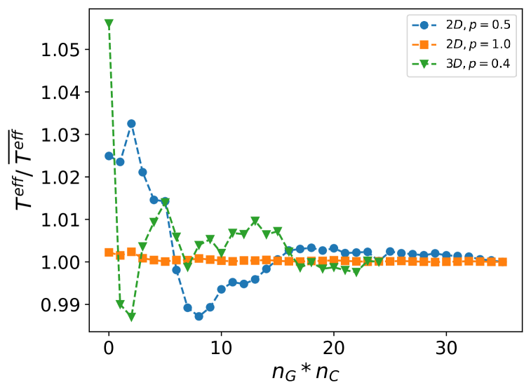
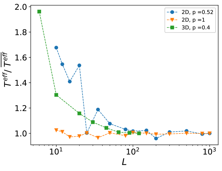
Figure 3: (Left) Influence of the number of realizations $N_{real}=n_{C}\times n_{G}$ on the average effective conductivity $T^{eff}$, normalized by $\overline{T^{eff}}$ for $N_{real}=1000$, for structured networks of size $512\times 512$ (2D) and $64\times 64\times 64$ (3D), and $\sigma^{2}_{\log T}=5$. (Right) Dependence of $T^{eff}$ on network size $L$, normalized by $\overline{T^{eff}}$ for the largest $L$, with $r=1$ and $\sigma^{2}_{\log T}=5$.

To explore the effects of geometric disorder on $T^{eff}$, the proportion $p$ was adjusted from values close to the percolation threshold to those representing full connectivity. The variance of the lognormal distribution, $\sigma^{2}_{\log T}$, was varied from zero (where all conductivities are uniform) to a highly heterogeneous scenario with $\sigma^{2}_{\log T}=5$. The simulation parameters are detailed in Table 1.

Table 1: Simulation Parameters

Parameter	Description	Values
$N_{x},N_{y},(N_{z})$	Dimensions	512 (2D), 64 (3D)
$r$	Radius	[1,..,5]
$p$	Proportion of conductive edges	[$p_{c}$,..,1]
$\sigma^{2}_{\log T}$	Variance of log conductivity	[0,.., 5]
$N_{real}$	Total number of realizations	900

IV Results

IV.1 Effective conductivity and power average exponent of 2D and 3D lattice RRN with r=1

In this section, we analyze the behavior of the average of the effective conductivity over the $N_{real}$, $\langle T^{eff}\rangle$, as a function of the connectivity parameter $p$ across structured Random Resistor Networks (RRNs) with $r=1$. The effective conductivity is computed for each parameter combination, and the results are presented in Fig. 4.

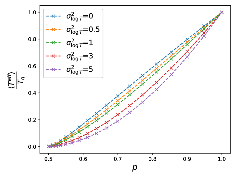
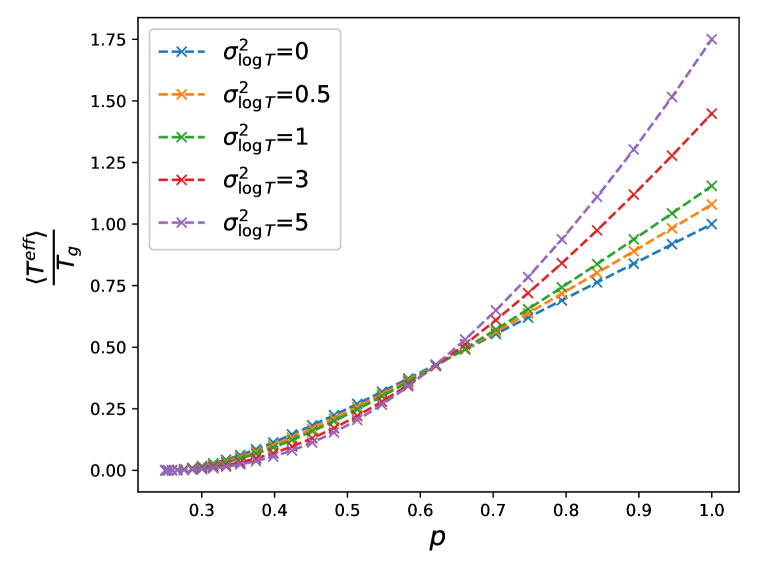
Figure 4: Arithmetic mean of $T^{eff}$ for structured RRNs: (left) in 2D, and (right) in 3D. In 2D networks, $T^{eff}$ decreases uniformly with increasing $\sigma_{\log T}^{2}$ across all $p$ values. Conversely, in 3D networks, $T^{eff}$ decreases when $\sigma_{\log T}^{2}$ increases at $p$ values below 0.63, and increases for $p$ values above this threshold. Notably, at full connectivity ($p=1$) for 2D and $p=0.63$ for 3D, $T^{eff}$ remains stable despite changes in variance, demonstrating effective compensation by the network’s geometry.

In 2D networks, effective conductivity consistently decreases with increasing $\sigma_{\log T}^{2}$, regardless of $p$. In 3D networks, the response to increasing $\sigma_{\log T}^{2}$ is more nuanced: effective conductivity decreases when $p$ is less than approximately 0.63, but increases for larger $p$ values.

The increase in variance, $\sigma_{\log T}^{2}$, depending on the network’s geometry, can lead to the formation of high-conductivity paths or to situations where the low conductivity of certain edges dominates the total flow. In opposition, at $p=1$ for 2D networks and at $p=0.63$ for 3D networks, $T^{eff}$ shows independence from the variance. This indicates a unique point of compensation where the network’s geometry or connectivity counterbalances the effects of increased variance.

The mean value of the power average exponent $\omega$, for a RRN with a given $\sigma_{\log T}^{2}$, computed from the numerical results of $T^{eff}$, are shown in Fig. 5.

At this stage, the exponent $\omega$ appears only as a particular data post processing, although its value may be estimated from theory for $p=1$. In that case, it was shown by numerical simulations that Eq. 14 provides a robust estimator of $T^{eff}$ even far from its theoretical validity limited to small log-conductivity variance. In present case, that treatment may be of interest if the exponent $\omega$ has little dependence with $\sigma_{\log T}^{2}$ and if its dependence with $p$ may be related to overall geometrical properties of the supporting connected network.

It can be observed that both set of curves depend on $\sigma_{\log T}^{2}$ at the notable exception for D=2, $p=1$ that corresponds to the exact result of Matheron (1967). In 3D, for $p$ close to 0.72, the apparent exponent $\omega$ vanishes, corresponding to an apparent flow dimension of 2. As exponent $\omega$ depends on the variance, it means that the mean-field hypothesis breaks down, even if it provides a quite good first approximations. As a preliminary conclusion, in spite of their simplicity, power-law averaging formulae can provide a fast determination of the average conductivity of a random network.

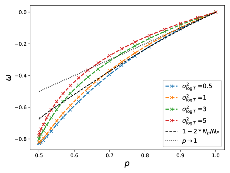
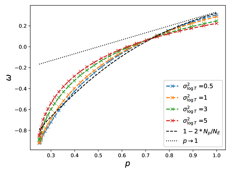
Figure 5: Power average exponent $\omega$, obtained from the results shown in Fig. 4, along with the approximation given by Eq. 12 (represented by the full black line). The results are presented for 2D (Left) and 3D (Right).

IV.2 Effective conductivity and power average exponent of 2D and 3D Structured RRN with $r>1$

In Sec. IV.1, we analyzed the behavior of the effective conductivity $T^{eff}$ in RRNs with a connectivity radius $r$ of 1. Extending this analysis, Fig. 6 presents $T^{eff}$ of RRNs where the connectivity radius $r$ extends beyond immediate neighbors ($r=5$), as a function of the connectivity degree $k$.

In 2D networks, for values of $k$ close to 3.2, $T^{eff}$ shows an independence from $\sigma_{\log T}^{2}$, analogous to the compensation point observed at $p=1$ ($k=4$) for $r=1$. As $k$ increases beyond this point, there is a pronounced increase in $T^{eff}$ with the variance.

For 3D networks, the compensation point similarly occurs around $k=3.2$. Beyond this threshold, $T^{eff}$ increases significantly faster with the variance for higher values of $k$ compared to 2D configurations. Getting a full understanding of the dependence of $\omega$ with $p$ will be the topic of another study.

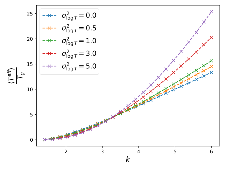
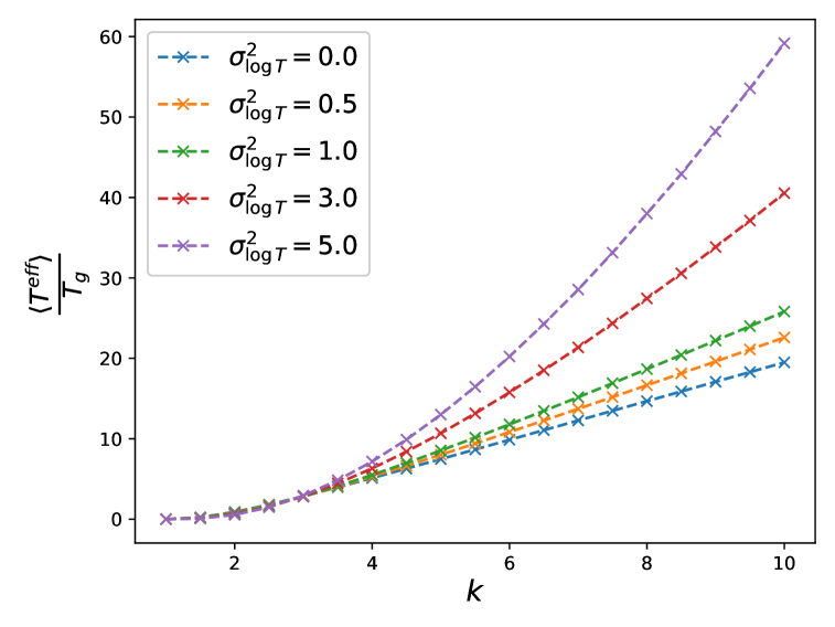
Figure 6: Variation of effective conductivity, $T^{eff}$, as a function of the mean degree $k$ for structured networks with a connectivity radius of $r=5$. The results are presented for 2D (left) and 3D (right).

The mean value of $\omega$, for a RRN with a given $\sigma_{\log T}^{2}$, is derived from the numerical results of $T^{eff}$ and displayed in Fig. 7 for networks with a connectivity radius of $r=5$. The exponent $\omega$ maintains stability even in networks with enhanced connectivity. Notably, the compensation point—where $\omega$ is independent of the variance at $k=4$ for both 2D and 3D networks.

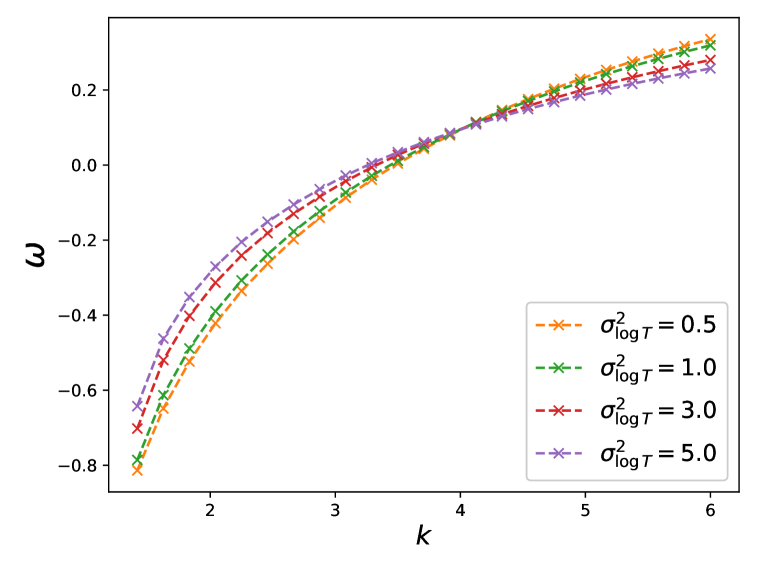
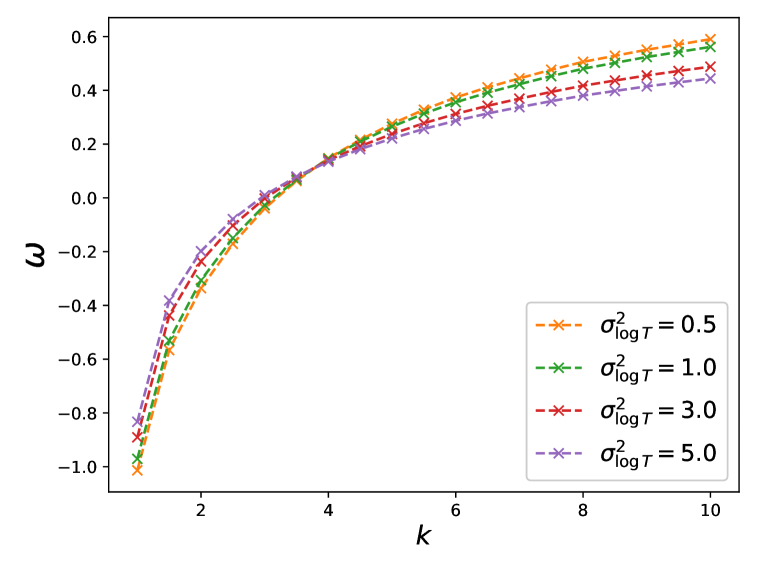
Figure 7: Power average exponent $\omega$ as a function of the mean degree $k$ for structured networks with a connectivity radius of $r=5$. The results, derived from the effective conductivity data shown in Fig. 6, are presented for 2D networks on the left and 3D networks on the right.

The results presented in Fig. 8 illustrates the variation of the power average exponent $\omega$ with respect to the mean degree $k$ in structured networks for different values of $r$, under conditions of high conductivity variance ($\sigma_{\log T}^{2}=5$). These observations are consistent with percolation theory and stochastic modeling predictions, highlighting a decreased influence of $r$ as $k$ increases. This trend emphasizes the percolation transition, wherein the network transitions to a state of effective homogeneity at larger scales. Notably, the dimensionality of 3D networks results in a more expansive percolation threshold, consequently enhancing the network’s overall transport capacity.

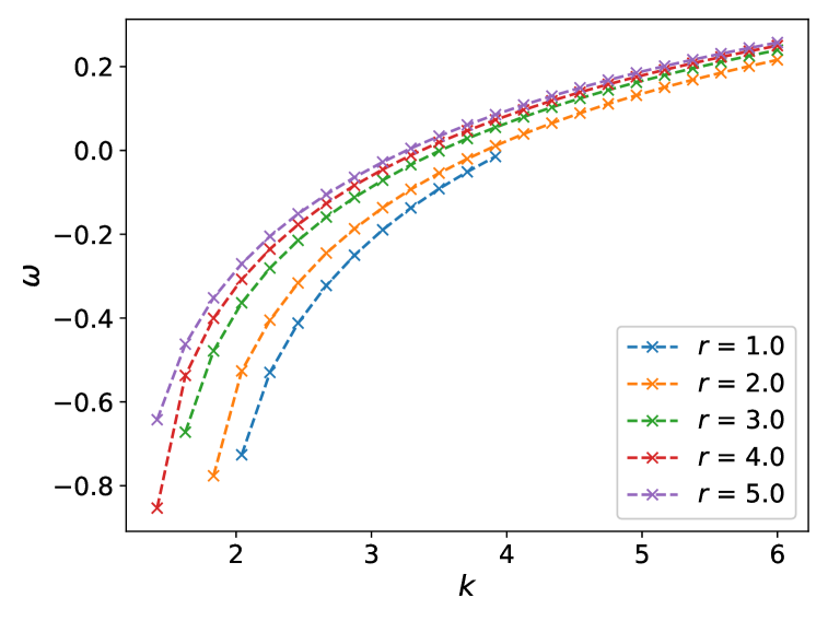
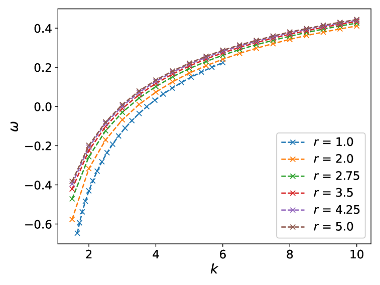
Figure 8: Variation of the power average exponent $\omega$ with the mean degree $k$ for structured networks, calculated for a high conductivity variance of $\sigma_{\log T}^{2}=5$. This set of graphs illustrates the influence of different connectivity radius on $\omega$ for 2D networks shown on the left and 3D networks on the right.

IV.2.1 Effective Conductivity of RRN with $p=1$

In this section, we present results for the effective conductivity $T^{eff}$ and the parameter $\omega$ for networks with r$>$1, where no edges have been removed. This setup provides a baseline understanding of the system’s behavior under maximal connectivity conditions. The difference between those networks with Erdős–Rényi networks, which are characterized by edges placed randomly between nodes with a fixed probability, is that the underlying 2D or 3D structure imposes a natural way of computing effective parameters with well-defined inlet and outlet boundary conditions.

The left panel of Fig. 9 depicts the variation of $T^{eff}$ as a function of the mean degree $k$, normalized by the geometric mean of the conductivity $T_{g}$. The relationship between $T^{eff}$ and $k$ suggests a power-law behavior, indicative of the network’s scaling properties under full connectivity. The right panel shows the parameter $\omega$ across different values of $k$, illustrating how changes in network connectivity influence flow characteristics even without the introduction of disorder by edge removal. For full networks with edges sharing the same conductivity, it can be showed that the overall conductivity scales with the square of its size. That size may be replaced by $r$ in the case of large structured networks of connectivity radius $r$. That is mainly due to the number of connections growing as the square of the number of nodes. That is confirmed in the left panel of Fig. 9 for $\sigma_{\log T}^{2}=0$. Interestingly, $\omega$ shows a rapid increase from values close to zero at low $k$, corresponding to the classical Matheron’s (1967) result for 2D networks, towards values approaching one, suggesting nearly parallel flow paths in the network as connectivity increases. This behavior highlights the transition from highly localized to more distributed flow as the network becomes increasingly connected, aligning with theoretical expectations for RRNs under varying connectivity and structural conditions.

The analysis of $T^{eff}$ and $\omega$ in fully connected networks sets the groundwork for understanding the impact of introducing disorder. It helps in distinguishing the effects of structural changes from those induced by altering connectivity and conductivity variance.

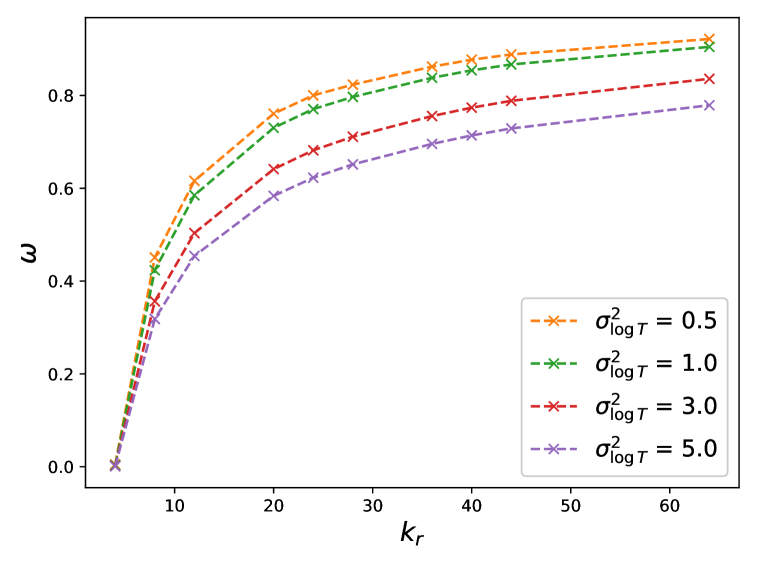
Figure 9: On the left, $T^{eff}$, of 2D RRN, normalized by the geometric mean $T_{g}$, is plotted against the mean degree $k$ on a logarithmic scale. The solid lines represent the fit to a power-law, with the power-law exponent listed in Table 2. On the right, the parameter $\omega$ is shown as a function of $k$, highlighting how network connectivity influences flow dynamics and transitions from localized to distributed flow regimes. These results establish a reference for the behavior of RRNs under maximum connectivity without edge removal.

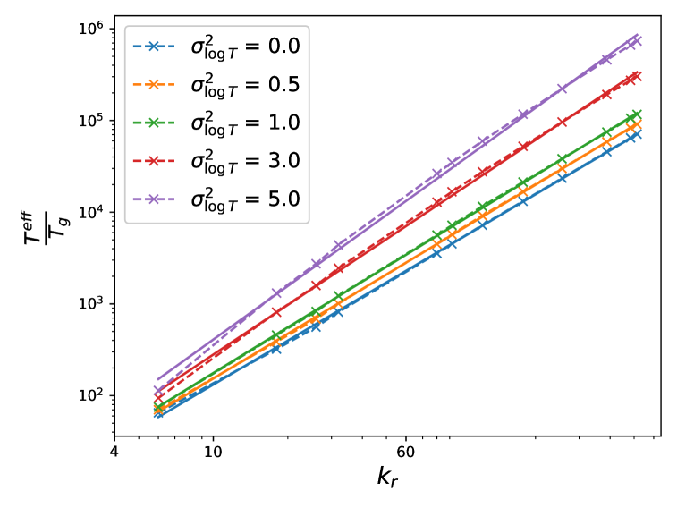
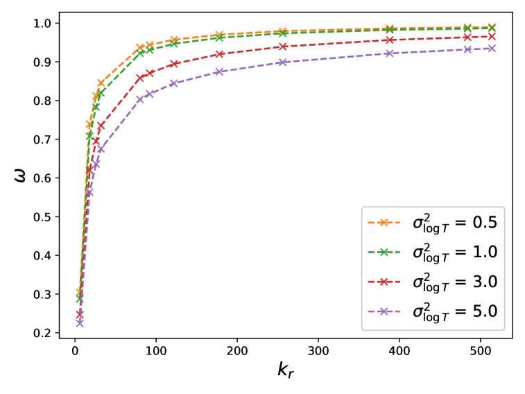
Figure 10: On the left, $T^{eff}$, of 3D RRN, normalized by the geometric mean conductivity $T_{g}$, is plotted against $k$ on a logarithmic scale. The solid lines represent the fit to a power-law, with the power-law exponent listed in Table 2. On the right, the parameter $\omega$ is shown as a function of $k$, highlighting how network connectivity influences flow dynamics and transitions from localized to distributed flow regimes.

Table 2: Fitting Parameters for the Power Law Relationship $\frac{T^{eff}}{T_{g}}=Ck_{r}^{t}$ for 2D and 3D Networks

Dimension	$\sigma^{2}_{\log T}$
	0.0	0.5	1.0	3.0	5.0
$t$ (2D)	1.88	1.96	2.04	2.32	2.56
$t$ (3D)	1.59	1.62	1.66	1.80	1.94

This comprehensive analysis of $T^{eff}$ and $\omega$ under varying degrees of connectivity provides insights into the foundational dynamics of flow in RRNs. By comparing these results with those obtained from networks with introduced disorder (edge removal), we can better understand the intrinsic properties of RRNs and their response to structural perturbations.

V Conclusions and discussion

Results about the interplay between the randomness of edge conductivity and the geometry of the supporting network are reported. Using perturbation methods quite popular in hydrologist community, we have a better understanding of the effect of the local conductivity randomness about the overall behaviour of the RRN. The role of the so-called resistance distance is highlighted, connections with up to date random graph/network theories can still lead useful and orginal results. The conductivity randomness dominates for well connected networks, while the topological disorder controls the overall behaviour of the system close to the percolation threshold. The results can be summarized as follows:

• A procedure to average RRN’s with respect to random conductivities fluctuations of the conductivity of its edges was set-up. The net result is an effective RRN with effective conductivities. Mathematically, it corresponds to estimating the harmonic average of the associated weighted laplacian matrix of the RRN. The averaged operator keeps a Laplacian structure.

• A suitable perturbation expansion was carried out. Strictly speaking, even with independent conductivities, the averaged RRN couples all the nodes, not just the input edges of the supporting RRN. However, up to the second order in a series expansion with respect to the logarithmic conductivity variance, the effective averaged RRN remains similar to the original one.

• The averaged RRN is characterized by a set of local effective conductivities $T_{ij}^{eff}$ that depends on the set of so-called resistance distances introduced in graph theory. A mean-field theory allows to propose a more robust estimation of the effective RRN using local power averaging of the local conductivities $T_{ij}$. The local averaging exponent depends on the geometry of the network.

• A relation between the so-called overall effective conductivity of the RRN and the statistical properties of the conductivity was derived up-to second order with respect to the Log conductivity variance, regardless on the geometry of the network. A robust extrapolation under the form of a power-averaging formula was established. A mean-field approach was proposed to provide a more solid foundation for this claim in Appendix B.

• Numerical simulations carried-out starting from Cartesian lattices in 2D or 3D are in correct agreement with that theoretical prediction, although some discrepancy may be observed close to percolation threshold.

• For large networks, the results are independent on the realization of both the network and the conductivity map, except close to the percolation threshold as it can be anticipated. So the proportion of active edges, (more generally connectivity parameter) and the input conductivity distribution variances are the most relevant parameters

• The corresponding averaging exponent $\omega$ is quite stable with the input variance and may be related to the proportion $p$ of active edges.

VI Perspectives

Several perspectives can be sketched:

• On the theoretical side, the overall structure of the harmonic average of the weighted laplacian should be studied for general log conductivity variance in order to justify that its structure remains essentially similar to the structure of $L_{0}$, with weights decreasing exponentially with the distance between vertices. In that direction, in analogy with averaging continuous Laplace equations with random coefficients, spectral methods appear as being a useful tool.

• In continuous up-scaling theories of Darcy’s law, a related approach involves analyzing the spectrum of the Laplacian matrix via Fourier transform techniques. Investigating the small frequency eigenvalues and eigenvectors of $\langle\mathbf{L}^{-1}\rangle^{-1}$, which describe the system’s overall behavior may be a possible avenue of investigation.

• The mean-field approach that allows to extrapolate a second-order expansion to the power law Eq. 1 must be tested numerically, as well as the approximations underlying the exponential solutions of Eqs. 22 and 29, by evaluating numerically the variations of the products $R_{ij}T_{ij}$ as long as the log conductivity variance is increased.

• Performing a similar study using as supporting network non-structured RRNs, closer to networks encountered in practice, in particular in geosciences applications.

• A related issue is to select various input conductivity distributions, indeed choosing identically log-normally distributed independent conductivity is a strong hypothesis.

• We addressed the averaging issue that is closely related in the continuous case to the up-scaling question (coarsening/homogenizing) of the flow equations. This is still relevant for RRN’s in which in analogy, the associated up-scaling issue may be related to a suitable grouping of vertices and edges. Methods of graph sparsification relying on the resistance distance were developed by previous authors [54] and may be useful for these up-scaling/degrees of freedom reduction purposes.

• Studying local flow, dissipation, and pressure drop distributions is essential for a deeper understanding of tracer transport, simplifying network models, and predicting the impact of specific edges on global flow, as well as addressing potential non-linearities in natural systems like karstic aquifers [52].

Appendix A Mean-field argument

We want to give some support to the power-law averaging extrapolated to higher log conductivity variance. We introduce $T_{gij}=exp\langle\log T_{ij}\rangle$ and $\sigma^{2}_{\log T_{ij}}\simeq\sigma^{2}_{ij}/\langle T_{ij}\rangle^{2}$. Combining equations 8 and 9, one gets up to second order using the resistance distance $R_{ij}$:

$$\langle\mathbf{L}^{-1}\rangle^{-1}_{ij}=\langle T_{ij}\rangle-R_{ij}\sigma^{2}_{ij}$$ (16)

So we get in terms of effective RRN:

$$T_{ij}^{eff}=\langle T_{ij}\rangle(1-\langle T_{ij}\rangle R_{ij}\sigma^{2}_{\log T_{ij}})$$ (17)

or equivalently up to second order:

$$T_{ij}^{eff}=T_{gij}+T_{gij}(1/2-\langle T_{ij}\rangle R_{ij})\sigma^{2}_{\log T_{ij}}$$ (18)

Because up to second order $\langle T_{ij}\rangle=\langle exp[\langle\log T_{ij}\rangle+\sigma_{\log T_{ij}}\zeta]\rangle\simeq T_{gij}(1+1/2\sigma^{2}_{\log T_{ij}}+\dots)$ where $\zeta$ is a random variable such that $\langle\zeta\rangle=0$ and $\langle\zeta^{2}\rangle=1$. The resistance distance between i and j is lower than 1/$T_{ij}$ because the current can flow through any path joining vertices i and j, including edge i j so we get the following inequality $0\leq T_{ij}R_{ij}\leq 1$.
Now, the main idea is to add heterogenity layer by layer by writing

$$T_{ij}=T_{gij}exp(\sum_{K=1}^{M}\zeta_{Kij}\sigma_{\log T_{ij}}/\sqrt{M})$$ (19)

where the $\zeta_{Kij}$ are independent random variables with respect to K, i and j such that $\langle\zeta_{Kij}\rangle=0$ and $\langle\zeta_{Kij}^{2}\rangle=1$. Central limit theorem states that when $M\rightarrow\infty$, the variable $\sum_{K=1}^{M}\zeta_{Kij}\sigma_{\log T_{ij}}/\sqrt{M}$ tends to a gaussian variable of mean 0 and of variance $\sigma_{\log T_{ij}}^{2}$. That implies that $T_{ij}$ is log-normal, corresponding to a product of a large number of positive random variables.

Then $T_{ij}^{eff,\ K}$ with $0\leq K\leq M$ is computed using equation 16 that can be applied recursively, by averaging over $\zeta_{kij}$ sequentially and using the fact that $\sigma_{\log T_{ij}}^{2}/N$ is small, and replacing $\bf{L_{0}}$ by $\mathbf{L}^{(K-1)}$ built using the K-1 previous heterogeneities. We obtain:

$$T_{ij}^{eff,\ K}=T_{gij}^{(K-1)}+T_{gij}^{(K-1)}(1/2-T_{gij}^{(K-1)}R_{ij}^{(K-1)})\sigma_{\log T_{ij}}^{2}/M$$ (20)

Our main hypothesis is to replace $\langle T_{ij}^{(K-1)}\rangle$ by $T_{ij}^{eff,\ K-1}$. That replacement means that the K-th conductivity fluctuation interacts through the effective medium corresponding to the K-1 preceding heterogeneity fluctuations. It corresponds to mean-field hypothesis. So we obtain:

$$T_{ij}^{eff,\ K}=T_{ij}^{eff,\ K-1}+T_{ij}^{eff,\ K-1}(1/2-T_{ij}^{eff,\ K-1}R_{ij}^{(K-1)})\sigma_{\log T_{ij}}^{2}/M$$ (21)

Setting $t=K/M$ and $dt=1/M$, letting $M\rightarrow\infty$, that equation can be written under the form of an ordinary differential equation given by:

$$\dfrac{dT_{ij}^{eff}(t)}{dt}=T_{ij}^{eff}(t)(1/2-T_{ij}^{eff}(t)R_{ij}(t))\sigma_{\log T_{ij}}^{2}$$ (22)

To be integrated for $t\in[0,1]$ with initial condition $T_{ij}^{eff}(t=0)=T_{gij}$. It remains to estimate the variations of $T_{ij}^{eff}(t)R_{ij}(t)$. The simplest hypothesis is to set $T_{ij}^{eff}(t)R_{ij}(t)\rightarrow T_{gij}R_{ij}(t=0)$. It corresponds to the product of the geometric mean of the local conductivity by the corresponding edge resistance, evaluated for the starting geometrically averaged network. That quantity is likely to depend mainly on the overall graph geometry and to present smooth variations. Such an hypothesis remains to be tested numerically. Using that assumption, the differential equation becomes linear and may be integrated, the desired value being its value for t=1:

$$T_{ij}^{eff}=T_{gij}exp[(1/2-T_{gij}R_{ij}(t=0))\sigma_{\log T_{ij}}^{2}]$$ (23)

For $T_{ij}$ log-normally distributed, it may be written under the equivalent power-averaging form.

$$T_{ij}^{eff}=\langle T_{ij}^{(1-2T_{gij}R_{ij}(t=0))}\rangle^{1/(1-2T_{gij}R_{ij}(t=0))}$$ (24)

That compact form can be used even if the input $T_{ij}$’s share another distribution, but with a more limited range of validity. Notice that for an edge such that $T_{gij}R_{ij}=1$, one obtains the harmonic average of the associated conductivity. That corresponds to an edge such that all the current flows through if its vertices are connected to a battery, a physically sound result. That product of the conductivity $T_{gij}$ and of the resistance $R_{ij}$ is likely to have quite smooth variations and to depend on the overall supporting network geometry.

Appendix B Derivation of effective conductivity Eq. 11 and Eq. 12 up to second order and of its associated power average extrapolation

In this Appendix, instead of determining local edges effective conductivities, that require quite heavy determination of a whole set of $R_{ij}$’s implying solving the number of edges $N_{E}$ times Laplace equations that can be costly, the focus is given about determining a single effective conductivity called $\lambda_{eff}$ such that the laplacian $\lambda_{eff}\bf T_{0}$ mimics the action of $\langle\bf{L}^{-1}\rangle^{-1}$.
The simplest criterion is to identify the corresponding trace by writing

$$Tr[\lambda_{eff}\mathbf{L_{0}}]=Tr\langle\bf{L}^{-1}\rangle^{-1}$$ (25)

which implies that the trace of the effective Laplacian is conserved. That requirement, which may seem arbitrary, may be heuristically justified by analogy with averaging flow in heterogeneous porous media or electrical conductivity when one identifies the energy dissipation associated to a uniform pressure or potential gradient $\simeq\sum_{edges<i,j>}L_{ij}=-TrL$ due to the structure of Laplacian matrices. So $\lambda_{eff}$ is given by $\lambda_{eff}=\dfrac{Tr\langle\bf{L}^{-1}\rangle^{-1}}{Tr\mathbf{L_{0}}}$.
In order to evaluate the dependence of $\lambda_{eff}$ with the conductivity heterogeneity variance, a reasoning similar to the one presented in Appendix A can be developed using the mean-field approach. Second order perturbation theory provides:

$$Tr\langle\mathbf{L}^{-1}\rangle^{-1}_{ij}=Tr\bf{L_{0}}-\sum_{edges}R_{ij}\sigma^{2}_{ij}$$ (26)

We can thus employ the same strategy than in Appendix A by adding randomness layer by layer, and expanding up to second-order using as average the preceding layer. We introduce thus the sequence

$$\lambda_{eff}^{K}=\dfrac{Tr\langle\bf{L}^{K,\ -1}\rangle^{-1}}{Tr\mathbf{L_{0}}}$$ (27)

In order to set-up the recursion, we can write:

$$\lambda_{eff}^{K}=\dfrac{Tr\langle\mathbf{{L}^{K,\ -1}}\rangle^{-1}}{Tr\langle\mathbf{{L}^{K-1,\ -1}}\rangle^{-1}}\times\lambda_{eff}^{K-1}$$ (28)

Then, the perturbation equation equation 26 can be used by replacing $\bf{L_{0}}$ by $\mathbf{L}^{K-1}$.

We add the following hypothesis: the log conductivity variance $\sigma^{2}_{Log(T_{ij})}=\sigma^{2}_{Log(T)}$ does not depend on the edge.
The machinery developed in Appendix A yields the following differential equation, once the mean-field hypothesis is assumed:

$$\dfrac{d\lambda^{eff}(t)}{dt}=\lambda^{eff}(t)(1/2-\dfrac{\sum_{edges\ ij}[T_{gij}^{eff}(t=0)]^{2}R_{ij}(t)}{\sum_{edges\ ij}T^{eff}_{gij(t)}})\sigma_{\log T}^{2}$$ (29)

Then, assuming that the nonlinear term retains its initial value at t=0, we obtain a linear equation that can be integrated.

$$\dfrac{d\lambda^{eff}(t)}{dt}=\lambda^{eff}(t)(1/2-\dfrac{\sum_{edges\ ij}T_{gij}^{2}R_{ij}}{\sum_{edges\ ij}T_{gij}})\sigma_{\log T}^{2}$$ (30)

Its solution is given by

$$\lambda^{eff}(t)=exp(1/2-\dfrac{\sum_{edges\ ij}T_{gij}^{2}R_{ij}}{\sum_{edges\ ij}T_{gij}})\sigma_{\log T}^{2}t$$ (31)

So finally at t=1.

$$\mathbf{L}^{eff}=\mathbf{L}_{g}exp(1/2-\dfrac{\sum_{edges\ ij}T_{gij}^{2}R_{ij}}{\sum_{edges\ ij}T_{gij}})\sigma_{\log T}^{2}$$ (32)

This justifies the relevance of power averaging in the log normal case with an exponent $\omega$ given by

$$\omega=1-2\dfrac{\sum_{edges\ ij}T_{gij}^{2}R_{ij}}{\sum_{edges\ ij}T_{gij}}$$ (33)

This overall exponent that appears to be a weighted average over the whole network of $T_{gij}^{2}R_{ij}$ is likely to be more stable than its local counter part of Appendix A.
In order to estimate $\omega$ in the cases presented in Sec. II.4, considering a large structured RRN of $N^{D}$ vertices in $D$ dimensions, corresponding to a finite difference approximation of a continuous Laplace equation using a $2D+1$ stencil. This corresponds to our lattice RRN with the parameter $r$ set to 1. Boundary effects are neglected due to the large value of $N$. We have to compute $\sum_{<i,j>}R_{ij}=\sum_{<i,j>}[{L_{0}}^{-1}_{ij}+{L_{0}}^{-1}_{ji}-{L_{0}}^{-1}_{ii}-{L_{0}}^{-1}_{jj}]$

That may be carried out by remarking $\mathbf{L_{0}}\mathbf{L_{0}}^{-1}=\mathbf{1}$, using the specific form of $\mathbf{L_{0}}$, that expression can be simplified. We obtain, using Eq. 33, $\omega=1-2/D$ with Eq. 11.
A similar analysis can be carried out in the case of percolation networks, built from full preceding lattices, in which a proportion $p$ of edges are kept, so changing $\mathbf{L_{0}}$ accordingly, removing finite clusters and using again the relation $\mathbf{L_{0}}\mathbf{L_{0}}^{-1}=\mathbf{1}$, combined with the specific form of $\mathbf{L_{0}}$ one gets:

$$\omega\approx 1-2\frac{N_{p}}{N_{E}}$$ (34)

Notice that strictly speaking such a formula is valid only at second order, even if using the mean-field argument appears to be a rather robust extrapolation. It is exact for 1D path graphs, and more generally for full D dimensional lattices were the result $\omega=1-2/D$ is recoverd.

Appendix C Analytical solution for path graphs

Consider a path graph of $N_{p}$ vertices ordered from 1 to $N_{p}$, listed in the order $v_{1}$, $v_{2}$, …, $v_{N_{p}}$ such that the edges are ($v_{i}$, $v_{i+1}$) where i = 1, 2, …, $N_{p}$ - 1. The set of equations of the RRN may be written as:

$$(1-\delta_{i,1})T_{i-1,i}(P_{i-1}-P_{i})+(1-\delta_{i,N_{p}})T_{i,i+1}(P_{i+1}-P_{i})=Q_{i}.$$

(35)

The two Kronecker symbols $\delta_{.,.}$ for i=1 or $N_{p}$, account for the special case of extreme vertices 1 and N. An elementary recursion permits to rewrite the RRN equations under the equivalent form:

$$\forall i=1,\cdots N_{p}-1,P_{i+1}-P_{i}=\frac{1}{T_{i,i+1}}\sum_{k=1}^{i}Q_{k}$$ (36)

Specializing this expression for i=$N_{p}$-1, we get

$$P_{N_{p}}-P_{N_{p}-1}=\frac{1}{T_{N_{p}-1,N_{p}}}\sum_{k=1}^{N_{p}-1}Q_{k}=-\frac{1}{T_{N_{p}-1,N_{p}}}Q_{N_{p}},$$

because $\sum_{j}Q_{j}=0$. That corresponds to the conservation relation Eq. 35 written at vertex $v_{N_{p}}$. The existence of a solution is thus ensured, that could be made explicit using the normalization condition $\sum_{j}P_{j}=0$. Averaging Eq. 36 over the disorder of the $T_{i,j}$, shows that the effective average RRN shares the same form than the original one, by replacing the set of conductivities by an effective set, sharing values given by the harmonic averages $\langle\frac{1}{T_{i,i+1}}\rangle^{-1}$, as it could be anticipated.
Coming back to the corresponding second-order expansion, considering source terms on the form $Q_{k}=Q(\delta_{kj}-\delta_{ki})$, the preceding solution Eq 36 shows that

$$[{L_{0}}^{-1}_{ij}+{L_{0}}^{-1}_{ji}-{L_{0}}^{-1}_{ii}-{L_{0}}^{-1}_{jj}]Q=(P_{i}-P_{j})=-\frac{Q}{\langle T\rangle}|j-i|$$ (37)

So

$$[{L_{0}}^{-1}_{ij}+{L_{0}}^{-1}_{ji}-{L_{0}}^{-1}_{ii}-{L_{0}}^{-1}_{jj}]=1/\langle T\rangle$$

for $j\in<i>$. That shows the consistency of the second-order expansion with the exact result for path graphs. The associated mean-field result leading to harmonic power averaging appears to be exact.

References

- Maxwell [1873] J. C. Maxwell, A treatise on electricity and magnetism, Vol. 1 (Oxford: Clarendon Press, 1873).
- Landau and Lifshitz [1960] L. Landau and E. Lifshitz, Electrodynamics of continuous media, Vol. 8 (Pergamon Press, 1960) p. 15.
- Hashin and Shtrikman [1962] Z. Hashin and S. Shtrikman, “A variational approach to the theory of the effective magnetic permeability of multiphase materials,” Journal of applied Physics 33, 3125–3131 (1962).
- Matheron [1967] G. Matheron, Eléments pour une théorie des milieux poreux (Masson, 1967).
- Torquato and Haslach Jr [2002] S. Torquato and H. W. Haslach Jr, “Random heterogeneous materials: microstructure and macroscopic properties,” Appl. Mech. Rev. 55, B62–B63 (2002).
- Gelhar [1993] L. W. Gelhar, Stochastic subsurface hydrology (Prentice-Hall, 1993).
- Dagan [1989] G. Dagan, Flow and transport in porous formations (Springer-Verlag GmbH & Co. KG., 1989).
- Indelman and Abramovich [1994] P. Indelman and B. Abramovich, “A higher-order approximation to effective conductivity in media of anisotropic random structure,” Water resources research 30, 1857–1864 (1994).
- Abramovich and Indelman [1995] B. Abramovich and P. Indelman, “Effective permittivity of log-normal isotropic random media,” Journal of Physics A: Mathematical and General 28, 693 (1995).
- Renard and De Marsily [1997] P. Renard and G. De Marsily, “Calculating equivalent permeability: a review,” Advances in water resources 20, 253–278 (1997).
- Jikov, Kozlov, and Oleinik [2012] V. V. Jikov, S. M. Kozlov, and O. A. Oleinik, Homogenization of differential operators and integral functionals (Springer Science & Business Media, 2012).
- Armstrong, Kuusi, and Mourrat [2019] S. Armstrong, T. Kuusi, and J.-C. Mourrat, Quantitative stochastic homogenization and large-scale regularity, Vol. 352 (Springer, 2019).
- King [1987] P. King, “The use of field theoretic methods for the study of flow in a heterogeneous porous medium,” Journal of Physics A: Mathematical and General 20, 3935 (1987).
- Quintard and Whitaker [1994] M. Quintard and S. Whitaker, “Transport in ordered and disordered porous media ii: Generalized volume averaging,” Transport in porous media 14, 179–206 (1994).
- Noetinger [1994] B. Noetinger, “The effective permeability of a heterogeneous porous medium,” Transport in porous media 15, 99–127 (1994).
- Noetinger and Gautier [1998] B. Noetinger and Y. Gautier, “Use of the Fourier-Laplace transform and of diagrammatical methods to interpret pumping tests in heterogeneous reservoirs,” Advances in Water Resources 21, 581–590 (1998).
- Hristopulos and Christakos [1999] D. Hristopulos and G. Christakos, “Renormalization group analysis of permeability upscaling,” Stochastic Environmental Research and Risk Assessment 13, 131–161 (1999).
- Nœtinger [2000] B. Nœtinger, “Computing the effective permeability of log-normal permeability fields using renormalization methods,” Comptes Rendus de l’Académie des Sciences - Series IIA - Earth and Planetary Science 331, 353 – 357 (2000).
- Teodorovich [2002] E. Teodorovich, “Renormalization group method in the problem of the effective conductivity of a randomly heterogeneous porous medium,” Journal of Experimental and Theoretical Physics 95, 67–76 (2002).
- Attinger [2003] S. Attinger, “Generalized coarse graining procedures for flow in porous media,” Computational Geosciences 7, 253–273 (2003).
- Eberhard, Attinger, and Wittum [2004] J. Eberhard, S. Attinger, and G. Wittum, “Coarse graining for upscaling of flow in heterogeneous porous media,” Multiscale Modeling & Simulation 2, 269–301 (2004).
- Stepanyants and Teodorovich [2003] Y. A. Stepanyants and E. Teodorovich, “Effective hydraulic conductivity of a randomly heterogeneous porous medium,” Water Resources research 39 (2003).
- Hristopulos [2020] D. T. Hristopulos, Random Fields for Spatial Data Modeling A Primer for Scientists and Engineers (Springer, 2020).
- Colecchio et al. [2020] I. Colecchio, A. Boschan, A. D. Otero, and B. Noetinger, “On the multiscale characterization of effective hydraulic conductivity in random heterogeneous media: a historical survey and some new perspectives,” Advances in Water Resources 140, 103594 (2020).
- King [1989] P. King, “The use of renormalization for calculating effective permeability,” Transport in porous media 4, 37–58 (1989).
- Berkowitz and Balberg [1993] B. Berkowitz and I. Balberg, “Percolation theory and its application to groundwater hydrology,” Water Resources Research 29, 775–794 (1993).
- Sahimi [2011] M. Sahimi, Flow and transport in porous media and fractured rock: from classical methods to modern approaches (John Wiley & Sons, 2011).
- Sahimi [1994] M. Sahimi, Applications of percolation theory (CRC Press, 1994).
- Renard and Allard [2013] P. Renard and D. Allard, “Connectivity metrics for subsurface flow and transport,” Advances in Water Resources 51, 168–196 (2013).
- Hunt, Ewing, and Ghanbarian [2014] A. Hunt, R. Ewing, and B. Ghanbarian, Percolation theory for flow in porous media, Vol. 880 (Springer, 2014).
- Maillot et al. [2016] J. Maillot, P. Davy, R. Le Goc, C. Darcel, and J.-R. De Dreuzy, “Connectivity, permeability, and channeling in randomly distributed and kinematically defined discrete fracture network models,” Water Resources Research 52, 8526–8545 (2016).
- Colecchio et al. [2021] I. Colecchio, A. D. Otero, B. Noetinger, and A. Boschan, “Equivalent hydraulic conductivity, connectivity and percolation in 2d and 3d random binary media,” Advances in Water Resources 158, 104040 (2021).
- Halihan and Wicks [1998] T. Halihan and C. M. Wicks, “Modeling of storm responses in conduit flow aquifers with reservoirs,” Journal of Hydrology 208, 82–91 (1998).
- Naughton et al. [2017] O. Naughton, P. Johnston, T. McCormack, and L. Gill, “Groundwater flood risk mapping and management: examples from a lowland karst catchment in ireland,” Journal of Flood Risk Management 10, 53–64 (2017), https://onlinelibrary.wiley.com/doi/pdf/10.1111/jfr3.12145 .
- Mayaud et al. [2019] C. Mayaud, F. Gabrovsek, M. Blatnik, B. Kogovšek, M. Petrič, and N. Ravbar, “Understanding flooding in poljes: A modelling perspective,” Journal of Hydrology 575, 874–889 (2019).
- Jeannin et al. [2013] P. Jeannin, U. Eichenberger, M. Sinreich, et al., “Karsys: a pragmatic approach to karst hydrogeological system conceptualisation. assessment of groundwater reserves and resources in switzerland,” Environmental Earth Sciences 69, 999–1013 (2013).
- Jeannin et al. [2021] P.-Y. Jeannin, G. Artigue, C. Butscher, Y. Chang, J.-B. Charlier, L. Duran, L. Gill, A. Hartmann, A. Johannet, H. Jourde, A. Kavousi, T. Liesch, Y. Liu, M. Lüthi, A. Malard, N. Mazzilli, E. Pardo-Igúzquiza, D. Thiéry, T. Reimann, P. Schuler, T. Wöhling, and A. Wunsch, “Karst modelling challenge 1: Results of hydrological modelling,” Journal of Hydrology 600, 126508 (2021).
- Gouy et al. [2024] A. Gouy, P. Collon, V. Bailly-Comte, E. Galin, C. Antoine, B. Thebault, and P. Landrein, “Karstnsim: A graph-based method for 3d geologically-driven simulation of karst networks,” Journal of Hydrology 632, 130878 (2024).
- Frantz et al. [2021] Y. Frantz, P. Collon, P. Renard, and S. Viseur, “Analysis and stochastic simulation of geometrical properties of conduits in karstic networks,” Geomorphology 377, 107480 (2021).
- Adler, Thovert, and Mourzenko [2013] P. M. Adler, J.-F. Thovert, and V. V. Mourzenko, Fractured Porous Media, Vol. 9780199666515 (Oxford University Press, 2013) p. 1 – 184.
- de Dreuzy, Méheust, and Pichot [2012] J.-R. de Dreuzy, Y. Méheust, and G. Pichot, “Influence of fracture scale heterogeneity on the flow properties of three-dimensional discrete fracture networks (dfn),” Journal of Geophysical Research: Solid Earth 117 (2012), https://doi.org/10.1029/2012JB009461, https://agupubs.onlinelibrary.wiley.com/doi/pdf/10.1029/2012JB009461 .
- Nœtinger and Jarrige [2012] B. Nœtinger and N. Jarrige, “A quasi steady state method for solving transient darcy flow in complex 3d fractured networks,” Journal of Computational Physics 231, 23–38 (2012).
- Hyman et al. [2019] J. D. Hyman, M. Dentz, A. Hagberg, and P. K. Kang, “Linking structural and transport properties in three-dimensional fracture networks,” Journal of Geophysical Research: Solid Earth 124, 1185–1204 (2019), https://agupubs.onlinelibrary.wiley.com/doi/pdf/10.1029/2018JB016553 .
- Noetinger [2023] B. Noetinger, “Random fields and up scaling, towards a more predictive probabilistic quantitative hydrogeology,” Comptes Rendus. Géoscience 355, 559–572 (2023).
- Journel et al. [1986] A. Journel, C. Deutsch, A. Desbarats, et al., “Power averaging for block effective permeability,” in SPE California Regional Meeting (Society of Petroleum Engineers, 1986).
- Desbarats [1992] A. Desbarats, “Spatial averaging of hydraulic conductivity in three-dimensional heterogeneous porous media,” Mathematical Geology 24, 249–267 (1992).
- Neuman and Orr [1993] S. P. Neuman and S. Orr, “Prediction of steady state flow in nonuniform geologic media by conditional moments: Exact nonlocal formalism, effective conductivities, and weak approximation,” Water resources research 29, 341–364 (1993).
- Charlaix, Guyon, and Roux [1987] E. Charlaix, E. Guyon, and S. Roux, “Permeability of a random array of fractures of widely varying apertures,” Transport in Porous Media 2, 31–43 (1987).
- de Dreuzy et al. [2010] J.-R. de Dreuzy, P. de Boiry, G. Pichot, and P. Davy, “Use of power averaging for quantifying the influence of structure organization on permeability upscaling in on-lattice networks under mean parallel flow,” Water Resources Research 46 (2010), https://doi.org/10.1029/2009WR008769, https://agupubs.onlinelibrary.wiley.com/doi/pdf/10.1029/2009WR008769 .
- Sanchez-Vila, Guadagnini, and Carrera [2006] X. Sanchez-Vila, A. Guadagnini, and J. Carrera, “Representative hydraulic conductivities in saturated groundwater flow,” Reviews of Geophysics 44 (2006).
- Dagan, Fiori, and Jankovic [2013] G. Dagan, A. Fiori, and I. Jankovic, “Upscaling of flow in heterogeneous porous formations: Critical examination and issues of principle,” Advances in Water Resources 51, 67–85 (2013), 35th Year Anniversary Issue.
- Noetinger [2013] B. Noetinger, “An explicit formula for computing the sensitivity of the effective conductivity of heterogeneous composite materials to local inclusion transport properties and geometry,” Multiscale Modeling & Simulation 11, 907–924 (2013).
- Klein and Randic [1993] D. J. Klein and M. Randic, “Resistance distance,” Journal of Mathematical Chemistry 12, 81–95 (1993).
- Spielman and Srivastava [2008] D. A. Spielman and N. Srivastava, “Graph sparsification by effective resistances,” in Proceedings of the fortieth annual ACM symposium on Theory of computing (2008) pp. 563–568.
- Stauffer and Aharony [2014] D. Stauffer and A. Aharony, Introduction to percolation theory: revised second edition (CRC press, 2014).
- De Wit [1995] A. De Wit, “Correlation structure dependence of the effective permeability of heterogeneous porous media,” Physics of fluids 7, 2553–2562 (1995).
- Romeu and Noetinger [1995] R. Romeu and B. Noetinger, “Calculation of internodal transmissivities in finite difference models of flow in heterogeneous porous media,” Water Resources Research 31, 943–959 (1995).
- Wang et al. [2017] M. Wang, Y.-F. Wang, Z.-F. Liu, X.-H. Wang, Y. Wang, and W.-D. Cao, “Finite analytic numerical method for three-dimensional quasi-laplace equation with conductivity in tensor form,” Numerical Methods for Partial Differential Equations 33, 1475–1492 (2017).
- Broutin et al. [2014] N. Broutin, L. Devroye, N. Fraiman, and G. Lugosi, “Connectivity threshold of bluetooth graphs,” Random Structures and Algorithms 44, 45 – 66 (2014).
- Knackstedt, Sahimi, and Sheppard [2000] M. A. Knackstedt, M. Sahimi, and A. P. Sheppard, “Invasion percolation with long-range correlations: First-order phase transition and nonuniversal scaling properties,” Phys. Rev. E 61, 4920–4934 (2000).
- Boschan and Noetinger [2012] A. Boschan and B. Noetinger, “Scale dependence of effective hydraulic conductivity distributions in 3d heterogeneous media: a numerical study,” Transport in porous media 94, 101–121 (2012).