SO(3)-Equivariant Neural Networks for Learning Vector Fields on Spheres

Abstract

Analyzing vector fields on the sphere, such as wind speed and direction on Earth, is a difficult task. Models should respect both the rotational symmetries of the sphere and the inherent symmetries of the vector fields. In this paper, we introduce a deep learning architecture that respects both symmetry types using novel techniques based on group convolutions in the 3-dimensional rotation group. This architecture is suitable for scalar and vector fields on the sphere as they can be described as equivariant signals on the 3-dimensional rotation group. Experiments show that our architecture achieves lower prediction and reconstruction error when tested on rotated data compared to both standard CNNs and spherical CNNs.

1 Introduction

It is well known that one of the reasons behind CNNs effectiveness is the use of convolutional layers that are translational equivariant, allowing weight sharing in the form of convolution kernels. In developing a neural network for signals on non-linear spaces such as the sphere, our convolution should respect the symmetries of our space of interest. Following the geometric blueprint outlined in [3], we have seen several examples of convolutional neural nets adapted to the sphere, such as [5] and [7] who independently developed spherical CNNs for rotation-invariant classification of scalar functions on the sphere. These are both based on replacing the usual Euclidean convolution layers with layers employing group convolution of the group $\operatorname{SO}(3)$ of 3-dimensional rotation matrices, which is the sphere’s symmetry group. Furthermore, [8] points out how vector fields on the sphere can be represented as equivariant signals on the group $\operatorname{SO}(3)$ of rotations, something which was also described in more generality and for general groups and tensors in [6] and [4]. Recently computationally efficient implementations of spherical CNNs that scale to more complex datasets have been presented [9].

In this paper, we showcase our take on how to construct a neural network whose output is a tensor on the sphere, with special attention to vector fields. As data, we use the ERA5 dataset to predict wind either from wind from an earlier time or from temperature at the same time. When predicting a tensor on a non-linear space, we are dealing with two kinds of equivariance. The model equivariance, which ensure that our model’s predictions are not dependent on how the sphere is embedded in $\mathbb{R}^{3}$, and the signal equivariance, in that we are considering signals on $\operatorname{SO}(3)$ together with an equivariance property so that they correspond to vector fields.

We present a group-convolution layer, which enforces the required symmetries of the data only after a full group-convolution on $\operatorname{SO}(3)$. Imposing the symmetry constraints after the group-convolution enables the possibility of adding non-equivariant activation functions, dropout layers, pooling layers, and the use of residual blocks, which can potentially result in a more expressive network. The ability to use residual blocks also allows for the development of UNet-type architectures, which can process the data at different scales of coarseness. linearities for more expressive outputs.

We remark that the current state-of-the-art models for weather prediction, such as GraphCast [18] and GenCast [20], are already models that take the geometry of the earth into account, through respectively a graph neural net on the sphere in a first case, and in using spherical normal distributions in the second case. Our model now opens up the possibility for weather prediction based on geometric convolutions, which can incorporate both scalar and tensor-valued data through the use of a smoothing operator. Furthermore, rotating observations is a simple way to obtain out-of-distribution examples to test our model with.

Compared to the models spherical-cnn [7], our network architecture does not use rotationally equivariant non-linearities, and can therefore also use more weights and have less trouble with dominating frequencies in the longitudinal direction and with signals of mixed type, see Remark 2.3 for details. As such, out network architecture, has more in common with s2cnn [5], unlike their classification experiments, we will also need to deal with preserving sample equivariance.

Our contributions can be summarized as follows:

• We present our take on $\operatorname{SO}(3)$ group-convolution networks that replace equivariant non-linearities with a smoothing operator, allowing more expressive activation functions to be used.

• We present a UNet-type architecture that can work with mixtures of scalar and vector field data throughout the network.

• We demonstrate that our $\operatorname{SO}(3)$-equivariant neural network outperforms previous work in experiments on global wind data forecasting and autoencoding.

2 Learning vector fields on the sphere

2.1 Differential tensors on the sphere and equivariant functions

Consider the sphere $S^{2}$ as a subspace of $\mathbb{R}^{3}$ comprised of unit vectors, and a differential tensor or a $\binom{i}{j}$-tensor as a section of the bundle $\Gamma(T^{*}(S^{2})^{\otimes i}\otimes T(S^{2})^{\otimes j})$. For example, scalar functions on $S^{2}$ are $\binom{0}{0}$-tensors, vector fields are $\binom{0}{1}$-tensors, and Riemannian metrics are $\binom{2}{0}$-tensors. By the hairy ball theorem [19] we cannot construct a global basis for the tangent bundle $TS^{2}$ and therefore we cannot represent these tensors globally as functions with values in a vector space. Instead, we will take advantage of the structure of $S^{2}$ as a homogeneous reductive space, and the structure of the group $\operatorname{SO}(3)$.

Any differential tensor on $S^{2}$ can be considered as an equivariant function on $\operatorname{SO}(3)$ called the associated function, where the form of the equivariance property depends on the type of differential tensor under consideration. This means that working on a specific class of equivariant functions on $\operatorname{SO}(3)$ is equivalent to working with differential tensors on $S^{2}$. We list a few examples here.

Example 2.1.

If $Z(\theta)$ is the matrix corresponding to a positive rotation by an angle $\theta$ around the $z$-axis then real functions $f:S^{2}\to\mathbb{R}$ are in unique correspondence with functions $\mathbf{f}:\operatorname{SO}(3)\to\mathbb{R}$ satisfying $\mathbf{f}(AZ(\theta))=\mathbf{f}(A)$, while vector fields $\xi:S^{2}\to TS^{2}$ are uniquely represented as functions $\boldsymbol{\xi}:\operatorname{SO}(3)\to\mathbb{C}$ satisfying the equivaraince condition $\boldsymbol{\xi}(A\cdot Z(\theta))=e^{-i\theta}\boldsymbol{\xi}(A)$, $A\in\operatorname{SO}(3)$. For a third example, we mention that any $\binom{l}{0}$-symmetric tensor $\Sigma:S^{2}\to(T^{*}(S^{2})^{\otimes i})$ is in unique correspondence with ${\boldsymbol{\Sigma}}:\operatorname{SO}(M)\to\mathbb{V}_{l}$ taking values in the space of complex polynomials $\mathbb{V}_{l}$ of degree $l$, which satisfy ${\boldsymbol{\Sigma}}(A\cdot Z(-\theta))(z)={\boldsymbol{\Sigma}}(A)(e^{-i\theta}z)$ for any $A\in\operatorname{SO}(3)$, $z\in\mathbb{C}$, $\theta\in\mathbb{R}$. We refer the reader to Appendix A for more details.

2.2 Vector field on $S^{2}$, signal equivariance, and model equivariance

Let $\operatorname{SO}(3)$ be the special orthogonal matrix group with unit Haar measure $\mu$. Consider the space $\mathcal{X}=L^{2}(\operatorname{SO}(3),\mathbb{C})$ of complex-valued square-integrable functions with respect to the inner product $\langle x,y\rangle_{L^{2}}=\int_{\operatorname{SO}(3)}x\bar{y}d\mu$. We define a left- and a right action of $\operatorname{SO}(3)$ on $\mathcal{X}$ by respectively $(\ell_{B}x)(A)=x(B^{-1}A)$ and $(r_{B}x)(A)=x(AB^{-1})$ for $A,B\in\operatorname{SO}(3)$.

Let $Z(\theta)$ be the matrix corresponding to a rotation around the $z$-axis by angle $\theta$. We can then define subspaces $\mathcal{X}_{n}\subseteq\mathcal{X}$ of functions satisfying $r_{Z(\theta)}x=e^{in\theta}x$, which will all be orthogonal to each other relative to the $L^{2}$-inner product. In particular, the subspaces $\operatorname{Re}\mathcal{X}_{0}$ and $\mathcal{X}_{1}$ uniquely correspond to respectively functions and vector fields on the sphere as outlined in Example 2.1. It follows that a neural network with weights $\psi$ which maps signals in $\mathcal{Y}$ to vector fields on $S^{2},$ $F_{\psi}:\mathcal{Y}\to\mathcal{X}_{1}$, must satisfy the property $r_{Z(\theta)}F_{\psi}(x)=e^{i\theta}F_{\psi}(x)$.

We will always consider neural networks where the input $\mathcal{Y}$ is a subspace of $\mathcal{X}$, more specifically, we consider either $\operatorname{Re}\mathcal{X}_{0}$ or $\mathcal{X}_{1}$. Ideally, we would like our network $F_{\psi}:~\mathcal{Y}~\to~\mathcal{X}$ not to depend on how we embed the sphere $S^{2}$ into euclidean space, i.e. a change in choice of the north pole and zero meridian line should not impact the ability of the network in making predictions. We can encode this independence by the equivariance $\ell_{A}F_{\psi}(x)=F_{\psi}(\ell_{A}x)$ for any $A\in\operatorname{SO}(3)$. In our experiments, data in $\mathcal{X}_{1}$ will represent wind data, while data in $\operatorname{Re}\mathcal{X}_{0}$ represents temperature.

In summary, we want the neural network to satisfy the following two properties:

1. signal equivariance: $r_{Z(\theta)}F_{\psi}(x)=e^{i\theta}F_{\psi}(x)$ for $x~\in~\mathcal{Y}$, $\theta\in\mathbb{R}$;

2. model equivariance: $\ell_{A}F_{\psi}(x)=F_{\psi}(\ell_{A}x)$ for any $x\in\mathcal{Y}$, $A\in\operatorname{SO}(3)$.

A natural way to achieve equivariance, in both (i) and (ii), is to construct the neural network using building blocks (layers), made of group-convolutions, activation function, and pooling, that are themselves equivariant.

2.3 Equivariant layers and group-convolutions

In order to construct equivariant linear layers, we need to introduce convolutions on the domain $\operatorname{SO}(3)$. We define the (left) convolution,

$$x*_{\ell}\psi(A)=\langle x,\ell_{A}\psi\rangle_{L^{2}},\qquad x,\psi\in\mathcal{X}.$$

Remark that if $L(x)=x*_{\ell}\psi$, then $L$ satisfies the model equivariance condition $L(\ell_{A}x)=\ell_{A}L(x)$. Furthermore, these are the only such equivariant linear maps from “the convolution is all you need” theorem, see Remark B.5. In order to efficiently compute these convolutions, we resort to describing them in the spectral domain, by making use of the Fourier transform on $\operatorname{SO}(3)$.

By combining the Peter-Weyl theorem, see Theorem IV.4.20 in [15] with representation theory of $\operatorname{SO}(3)$, e.g. [21], we can use the coefficient of the irreducible representations known as the Wigner D-matrices $D^{l}$, $l=0,1,2,\dots$ as a basis for $\mathcal{X}=L^{2}(\operatorname{SO}(3),\mathbb{C})$. For each $l=0,1,2,\dots$, the coefficient functions of $D^{l}~=~(D_{m,n}^{l}):\operatorname{SO}(3)~\to~U(2l+1)$, which are commonly indexed from $-l$ to $l$, satisfy the orthogonality condition

$$\langle D_{m,n}^{l},D_{b,c}^{a}\rangle_{L^{2}}=\frac{1}{2l+1}\delta_{l,a}\delta_{m,b}\delta_{n,c}.$$

Furthermore, the D-matrices satisfy the condition $r_{Z(\gamma)}D_{m,n}^{l}~=~e^{in\gamma}D_{m,n}^{l}$, meaning that

$$\mathcal{X}_{n}=\operatorname{span}_{\mathbb{C}}\{D^{l}_{m,n}\}^{-l\leq m\leq l}_{l=0,1,2,\dots}.$$

Thus for any function $x\in\mathcal{X}$ we can write the corresponding Fourier expansion

$$\mathscr{F}(x)=\hat{x}=(\hat{x}_{m,n}^{l})_{I}\qquad x=\sum_{I}\hat{x}_{-m,-n}^{l}D_{m,n}^{l}.$$ (2.1)

with $I$ being the indexing set of triples $(l,m,n)$ with $l$ a non-negative integer and $-l\leq m,n\leq l$. Fourier coefficients of the convolution $x*_{\ell}\psi$ can then be directly computed using the Fourier transform

$$\widehat{x*_{\ell}\psi}_{m,n}^{l}=\frac{1}{2l+1}\sum_{s=-l}^{l}\hat{x}_{m,s}^{l}\overline{\hat{\psi}_{n,s}^{l}},\qquad x,\psi\in\mathcal{X}.$$

Observe that if $x\in\mathcal{X}_{p}$, then it holds that $\widehat{x*_{\ell}\psi}_{m,n}^{l}~=~\frac{1}{2l+1}\hat{x}_{m,p}^{l}\overline{\hat{\psi}_{n,p}^{l}}$, $x,\psi\in\mathcal{X}$, so that if $\psi$ is playing the role of weights in the neural network, only its Fourier coefficients $\hat{\psi}_{n,q}^{l}=\hat{\psi}_{n}^{l}$ need to be taken into consideration, as when $s\neq p$ no contribution is given to the summation. We write the inverse of the Fourier transform as $\mathscr{F}^{-1}(y_{m,n}^{l})_{I}$.

Remark 2.2.

By using our own version of the approach given in [14], we can use the usual FFT and iFFT in three dimensions for $2\pi$-periodic signals for fast computations of the Fourier transform on $\operatorname{SO}(3)$. For exact formulation, see Appendix B. We make the convention of negative indexing in (2.1) to simplify the correspondence with the usual Fourier coefficients.

2.4 Layers of our model

We will now describe the layers that make up our proposed architecture, see also Figure 1. If $\sigma$ is a non-linearity, we can define

$$PreL(x)=\sigma(x*_{\ell}\psi).$$

This layer will satisfy the model equivariance since the left action on $\mathcal{X}$ is defined through pre-composition, while the non-linearity is used in post-composition. On the other hand, neither the convolution nor the non-linearity will preserve the signal equivariance. Hence, if we want to define layers $L:\mathcal{X}_{p}\to\mathcal{X}_{q}$ which respects signal equivariance, then we will need to include a smoothing operator, following the terminology in [2], which is an orthogonal projection $\mathscr{S}_{q}:\mathcal{X}\to\mathcal{X}_{q}$ defined by $\mathscr{S}_{q}(x)=\frac{1}{2\pi}\int_{0}^{2\pi}e^{iq\theta}r_{Z(-\theta)}x\,d\theta$, which satisfies $\mathscr{S}_{q}(x)=\delta_{p,q}x$ for $x\in\mathcal{X}_{p}$, $p\in\mathbb{Z}$, and hence for a general signal $x\in\mathcal{X}$ the computation in the spectral domain boils down to

$$\widehat{\mathscr{S}_{q}x}=(\hat{x}_{m,q}^{l}\delta_{n,q})_{I}.$$

As a consequence, the smoothing operator can be applied by simply restricting the signal on a subset of the Fourier coefficients, rather than performing the integral in the spatial domain. Since smoothing operators commute with the left action, we can define our convolution layer $L:\mathcal{X}_{p}\to\mathcal{X}_{q}$ as

$$L(x)=\mathscr{S}_{q}\left(\sigma\left(\mathscr{F}^{-1}\left(\tfrac{1}{2l+1}\hat{x}_{m,p}^{l}\overline{\psi_{n}^{l}}\right)_{I}\right)\right),$$

where $\psi_{n}^{l}$, $-l\leq n\leq l$ are the weights to be learned. We will only use $p,q=0,1$ in our examples, as these correspond to the type of data we are interested in.

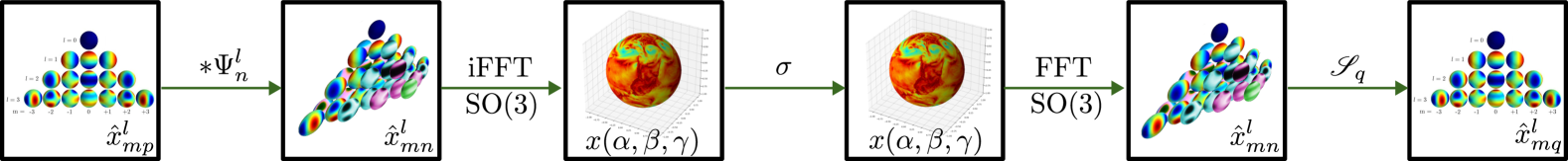
Figure 1: The proposed $\operatorname{SO}(3)$-equivariant layer, mapping a $p$-equivariant signal to a $p$-equivariant signal. It consists of a group-convolution, inverse Fourier transformation ($\operatorname{SO}(3)$), nonlinearity, Fourier transformation ($\operatorname{SO}(3)$) and smoothing in $p$. A scalar field is encoded with $p=0$ while $p=1$ corresponds to a vector field.

Remark 2.3.

If we choose a rotationally equivariant non-linearity, i.e., one satisfying $\sigma(e^{i\theta}\cdot)=e^{i\theta}\sigma(\cdot)$, then we can also create a layer $L:\mathcal{X}_{p}\to\mathcal{X}_{q}$

$$L(x) =\sigma\left(\mathscr{S}_{q}\left(\mathscr{F}^{-1}\left(\tfrac{1}{2l+1}\hat{x}_{m,p}^{l}\overline{\psi_{n}^{l}}\right)_{I}\right)\right)$$

$$=\sigma\left(\mathscr{F}^{-1}\left(\tfrac{1}{2l+1}\hat{x}_{m,p}^{l}\overline{\psi^{l}}\delta_{q,n}\right)_{I}\right).$$

We remark the illustrative special case that if $\hat{x}_{m,p}^{l}=0$ for $m\neq m_{1}$ and $y=L(x)$, then $\hat{y}_{m,q}^{l}$ will also vanish when $m=m_{1}$. In general, if the size of $(x_{m_{1},p}^{l})_{l=0,1,\dots}$ dominate compared to the other values of $m$, then this $m_{1}$ will also dominate the output unless sufficiently compensated for by the weights.

Another problem is with signals of mixed type, as while a rotationally equivariant non-linearity preserves $\mathcal{X}_{p}$, it will not preserve $\mathcal{X}_{p}+\mathcal{X}_{p_{2}}$, and hence with mixed inputs, there will be some final smoothing required to get the desired outputs.

Remark 2.4.

Smoothing after every layer, as opposed to only performing it as a last step in the network, comes at a cost in terms of working with fewer Fourier coefficients. This is however a trade-off in that such a network requires not only fewer weights but also allows higher throughput on the GPU, compared to only applying smoothing at the final output. It also enables the ability to use non-equivariant nonlinearities and residual blocks when dealing with data of different natures (e.g. scalar, vector, …) without compromising the equivariance of the signal.

3 The proposed network architecture

In this section, we aim to describe the proposed architecture in more detail. The pytorch implementation of the network and the experiments can be found at
https://git.app.uib.no/francesco.ballerin/gdl-wind.

3.1 Filters

An $\operatorname{SO}(3)$-(left) equivariant filter in our proposed architecture is computed in the Fourier domain in the form

$$\hat{y}_{m,n}^{l}=\frac{1}{2l+1}\sum_{s=-l}^{l}\hat{x}_{m,s}^{l}\hat{\psi}_{n,s}^{l},\qquad x,\psi\in\mathcal{X},$$

where $y\in\mathcal{X}$ is the output function with Fourier coefficients $\hat{y}_{m,n}^{l}$. We can drop the complex conjugation on the weights $\psi_{n,s}^{l}$ as learning on $\psi_{n,s}^{l}$ is equivalent to learning on $\overline{\psi_{n,s}^{l}}$.

In the specific cases of $x\in\mathcal{X}$ being a band-limited signal, limited by order $L$, either $x\in\mathcal{X}_{0}$ or $x\in\mathcal{X}_{1}$, the filter coefficients $\psi_{n,s}^{l}$ will be one dimension lower as there will be a natural restriction to $s=0$ or $s=1$. In these cases, the weights can be encoded as an array of $L*(L+2)+1$ complex values for $x\in\mathcal{X}_{0}$ and $L*(L+2)$ complex values for $x\in\mathcal{X}_{1}$.

3.2 Nonlinearities / activation functions

The use of a smoothing operator following the nonlinearity guarantees that the output signal is in $x\in\mathcal{X}_{p}$, thus possessing the correct signal-equivariance we are interested in (which in our experiments are $p=0$ for scalar fields and $p=1$ for vector fields). We can therefore use any nonlinearity we please in the spatial domain, and not restrict ourselves to nonlinearities that preserve the signal equivariance of choice.

Nonlinearities in the spectral domain are known not to mix frequencies belonging to two different orders ($l$ indexes) but only Fourier coefficients within the same order. Due to this behavior, we compute the activation functions in the spatial domain.

All implementations of our proposed architecture use weighted leaky ReLUs for both the real and the imaginary parts of the signal.

3.3 Spectral pooling

Pooling can be achieved by truncating the order of the Fourier series of Wigner-D-matrices following a nonlinearity in the spatial domain.

Other types of poolings have been suggested, such as performing pooling in the spatial domain, which is only approximately equivariant, or performing a weighted pooling to account for the surface area measure as outlined in [7].

3.4 UNet-like Architecture

We introduce a UNet-like architecture for signals $x\in\mathcal{X}_{p}$, with pooling performed in the spectral domain to produce a coarser signal to manipulate in the ”deeper” layers of the network (see Figure 2). The unpool component of the network is performed by padding the coarser signal with zeros and stacking the features with the residues from the residual block.

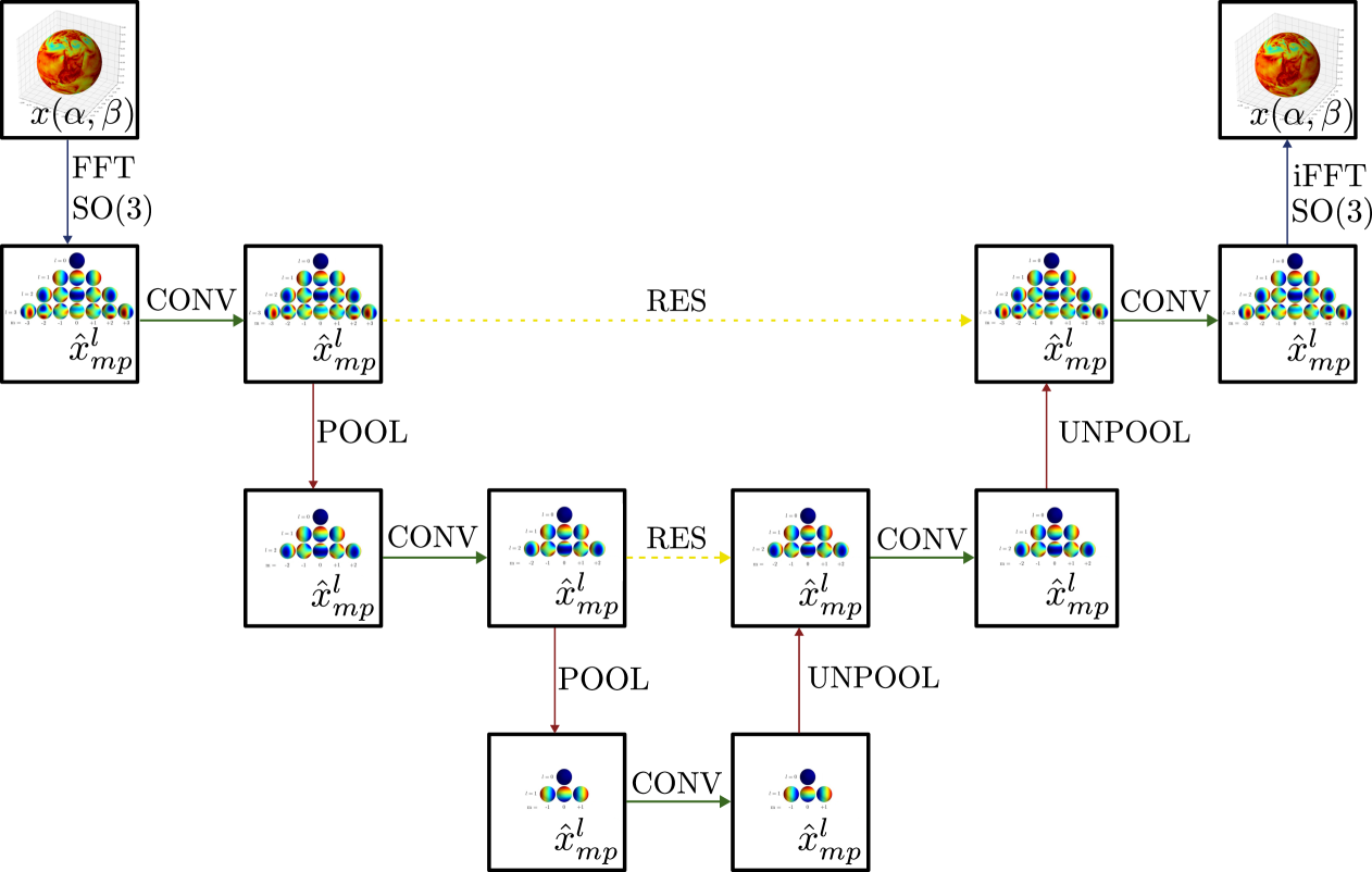
Figure 2: The proposed $\operatorname{SO}(3)$-equivariant UNet-type architecture. CONV layers as presented in Section 2.3 and as visualized in Figure 1. Yellow dotted lines (RES) correspond to the residual blocks. Pool and Unpool are performed in the spectral domain.

3.5 Loss function on $S^{2}$

The loss chosen to be used during training is a weighted MSE loss, weighted by a factor $\sin(\beta)^{2}$ to account for the surface area measure on $S^{2}$, in correspondence with the performance measure. For two vector signals on the sphere X, Y in lon/lat coordinates $\alpha$, $\beta$ the weighted MSE loss is explicitly defined as

$$\mathcal{L}(\textbf{X},\textbf{Y})=\sum_{\alpha,\beta}(\sin\beta)^{2}[(x_{1}^{\alpha\beta}-y_{1}^{\alpha\beta})^{2}+(x_{2}^{\alpha\beta}-y_{2}^{\alpha\beta})^{2}].$$

3.6 Equivariance by rotation

All our proposed models guarantee equivariance by $\operatorname{SO}(3)$ left-actions up to numerical errors, i.e. if $F:\mathcal{X}\to\mathcal{X}$ is our proposed network and $\ell_{B}$, where $B\in\operatorname{SO}(3)$, is a left -action, then $\ell_{B}F(x)=F(\ell_{B}x)$. In other words, applying a 3D rotation to the input or to the output produces the same result. This property is not held by a classical CNN, as the translational equivariance on the Euclidean domain does not correspond to a rotational equivariance on the sphere (the only exception being the class of rotations $Z(\theta)$ which rotate $S^{2}$ around the $z$-axis). This stark difference can be appreciated with an example in Table 1.

Model	Ground truth	Predicted $\beta=0$	Predicted $\beta=\frac{\pi}{4}$	Rotation error
CNN
Ours
0 km/h 28 km/h

Table 1: The table shows a comparison between an $\operatorname{SO}(3)$-equivariant Neural Network and a CNN in the task of predicting vector fields. Both Networks have been trained without data augmentation, corresponding to $\operatorname{SO}(3)$ group actions. For visualization purposes, only the magnitude is displayed. The second column shows the ground truth (same for both rows) for a vector field inside the training distribution (not data-augmented). The third column shows the predicted result for both Networks. The fourth column shows the prediction when the sample in input is rotated by Euler angle $Y(\pi/4)\in\operatorname{SO}(3)$, visualized in the original orthonormal frame for visualization purposes. The last column shows the error that is incurred when performing such a rotation.

4 Experiments

To evaluate the proposed architecture, we conducted a proof-of-concept experiment based on meteorological data, in the form of vector fields and scalar fields (wind speed/direction and temperatures). This preliminary study aimed to validate the architecture’s functionality and compare the performances of our proposed $SO(3)$-equivariant architecture with a classical CNN architecture and an example of spin-weighted spherical CNN [9], in particular when dealing with data augmented by applying $\operatorname{SO}(3)$ rotations. All three models have been trained with a comparable number of parameters, by tuning the number of features in use in the hidden layers, and similar architectures.

4.1 Performance measure

For two vectors $\textbf{x},\textbf{y}$ belonging to the same tangent space on $S^{2}$ we can measure their distance by the $\ell_{2}$ norm on $\mathbb{R}^{2}$, $d(\textbf{x},\textbf{y})=\sqrt{(x_{1}-y_{1})^{2}+(x_{2}-y^{2})^{2}}$. This, together with the surface area element $dS=\sin\beta d\alpha d\beta$, induces a natural distance for vector fields on the sphere

$$\mathcal{D}(\textbf{X},\textbf{Y})=\int_{S^{2}}\sqrt{(x_{1}^{\alpha\beta}-y_{1}^{\alpha\beta})^{2}+(x_{2}^{\alpha\beta}-y_{2}^{\alpha\beta})^{2}}dS$$

which can be interpreted as the average deviation in magnitude between vectors at the same point. In the discrete setting of a longitude/latitude grid with $A$ meridians and $B$ parallels is

$$\mathcal{D}(\textbf{X},\textbf{Y})=\frac{1}{AB}\sum_{\alpha,\beta}\sin\beta\sqrt{(x_{1}^{\alpha\beta}-y_{1}^{\alpha\beta})^{2}+(x_{2}^{\alpha\beta}-y_{2}^{\alpha\beta})^{2}}.$$

4.2 Dataset

The data used during training, validation, and testing is a subset of the ERA5 hourly dataset [13] concerning temperature at 2m (2m temperature) and wind speed and direction at 100m (100m u-component of wind, 100m v-component of wind).

For training and model selection we have extracted a subset of 52 datapoints per year for both wind and temperature, corresponding to temporally equally distanced weekly measurements. Our choice to consider such a coarse dataset is due to the excessively long training time on the full dataset. Years from 2000 to 2009 (included) have been used for training, while the years 2020 and 2021 have been used for validation and model selection. When performing model selection the validation dataset in the canonical rotation was used if the training was performed on non-rotated data, while a fixed rotated validation dataset was used if training was performed on rotated copies of the training data.

For testing, we have considered a subset of 365 datapoints for each 2022 and 2023, corresponding to daily measurements at 12:00 noon. When testing a model the test dataset in the canonical rotation has been used if training was performed on non-rotated data, while a fixed randomly rotated test dataset has been used if training was performed on rotated copies of the training data.

4.3 Future wind prediction

The task of the models in this experiment is to predict wind speed and direction at $t$+24hrs given wind speed and direction at time $t$, providing a proof of concept for an equivariant vector-to-vector neural network. The baseline model is a CNN UNet [22] with depth 4 and layers made of two 3x3 convolutions with ReLU, for a total model weight of 29.62 MB. Our proposed $\operatorname{SO}(3)$-equivariant model is a UNet-type architecture where the convolutional layers of the CNN have been substituted for $\operatorname{SO}(3)$-(left)equivariant fully connected layers with smoothing operator at $n=1$, for a total model weight of 26.85 MB. Our implementation of the spherical CNN by Esteves et al. [9], also as a UNet-type architecture, has a total weight of 28.42 MB.

A detailed description of the UNet-type architecture, including pooling and activation functions, can be found in Appendix 3.

4.4 Temperature to wind estimation

The task of the models in this experiment is to predict wind speed and direction at time $t$ given the temperature at the same time $t$, providing a proof of concept for an equivariant scalar-to-vector neural network. The models used in this test are the same ones employed in the ”future wind prediction” task, with the only difference being the change of smoothing operator (at $n=0$ for all layers except the last one). We did not run this task on the spherical CNN as the lack of a smoothing operator layer made it incompatible with the UNet-type architecture which has mixed inputs for $p\neq q$ ($p=0$ for temperature, and $q=1$ for wind).

4.5 $\operatorname{SO}(3)$-equivariant wind autoencoder

The task of the models in this experiment is to perform data compression on vector fields by employing autoencoders to fit the data into a fixed latent space of a given dimension. The baseline model is a CNN autoencoder of 8+8 layers with latent dimension 512, resulting in a total model weight of 7.52 MB. Our proposed $\operatorname{SO}(3)$-equivariant autoencoder exchanges the convolution/deconvolution layers in favor of $\operatorname{SO}(3)$-(left)equivariant flayers, resulting in a model with a weight of 10.55 MB. Analogously to the Task 4.3 we have adapted our implementation to reflect the architecture proposed by Esteves et al. [9] and increase the number of hidden features to achieve a similar number of weights, for a total model weight of 6.43 MB.

4.6 Results

Table 2 shows the results for different types of tasks and data types (vector fields in $\mathcal{X}_{1}$ for wind and scalar fields in $\operatorname{Re}\mathcal{X}_{0}$ for temperature), differentiating between data augmentation on $\operatorname{SO}(3)$ rotations has been used in training and/or test. Figure 3 shows a comparison between the different models under examination in the task of wind prediction $\mathcal{X}_{1}\to\mathcal{X}_{1}$ when training on a dataset of variable size (from 1 to 10 years between 2000 and 2009).

Although the models had a comparable size in terms of number of parameters, they differed when comparing training speeds. For example, when considering the Task 4.3, our implementation of a spherical CNN was roughly 280 times slower than a classical CNN, while our proposed architecture was roughly 6850 times slower when taking into consideration the number of samples in a minibatch. This is due, on one hand, to the efficient out-of-the-box implementation for classical CNNs, which easily scale with the batch dimension, and on the other hand, to the fact that the Fourier coefficients in our proposed architecture have an extra dimension compared to spherical CNNs that slows down the Fourier transform computation. It is also worth mentioning that some of the speed during both the forward pass and the backward pass could be recovered by writing efficient low-level implementations of both the $\operatorname{SO}(3)$-convolutions and the $\operatorname{SO}(3)$-FFT. This was however out of the scope of this work.

Task	Model	NR/NR	NR/R	R/R
Wind to wind	CNN	.042927	.060793	.041455
	sCNN	.049591	.049228	.049055
	Ours	.045662	.045254	.045187
Temp. to wind	CNN	.048644	.092276	.063269
	Ours	.055538	.055306	.055235
Wind autoencoder	CNN	.069540	.084329	.073603
	sCNN	.063897	.063594	.064374
	Ours	.063609	.063329	.062071

Table 2: Average performance of a convolutional UNet (CNN), our implementation of spherical CNN network (sCNN), and our proposed architecture (Ours) evaluated on the test dataset (2022, 2023). In this table R = rotated, NR = non-rotated and X / Y denotes that the network was trained on X and evaluated on Y. Training, both in the R and NR case, was performed with years 2000 to 2009. Rotations are computed as described in Section 4.2.

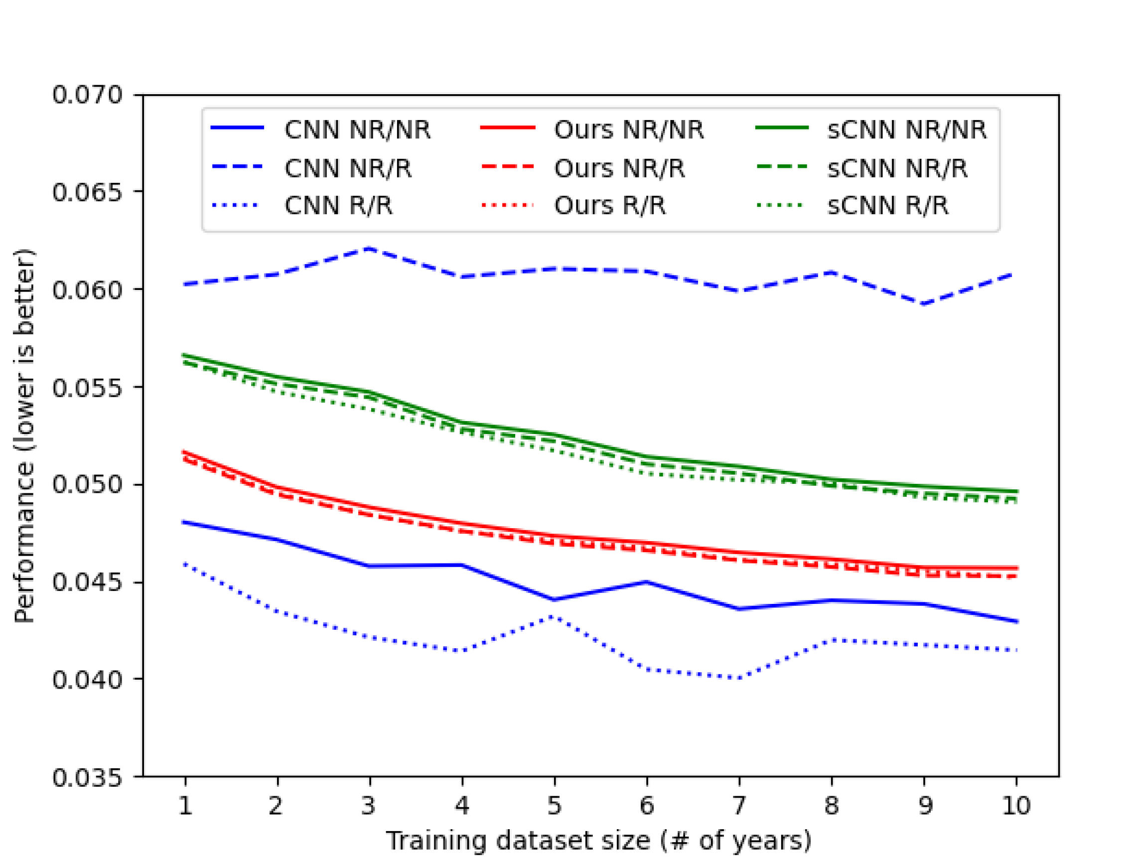
(a) Wind to Wind t+24h prediction.

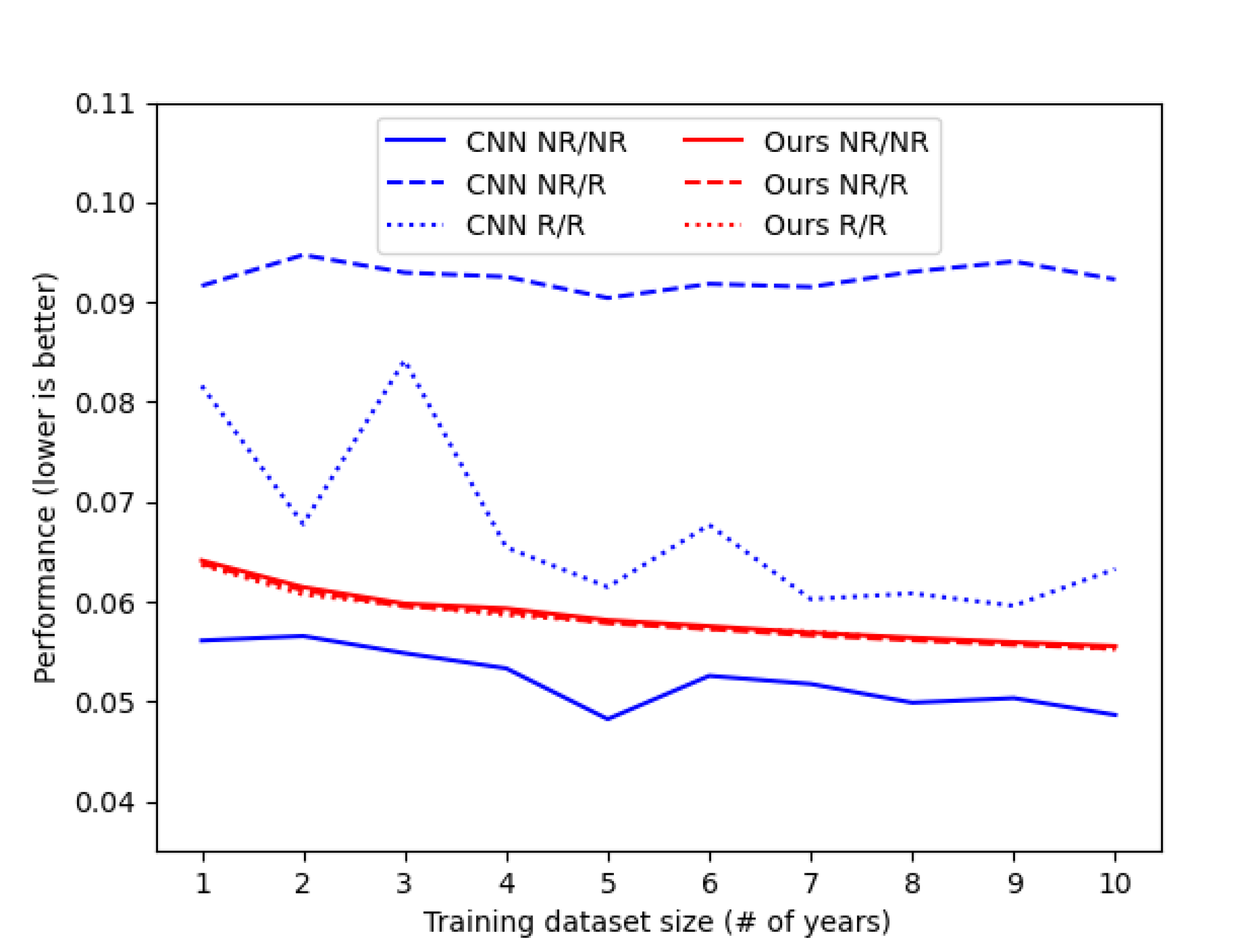
(b) Temperature to Wind estimation.

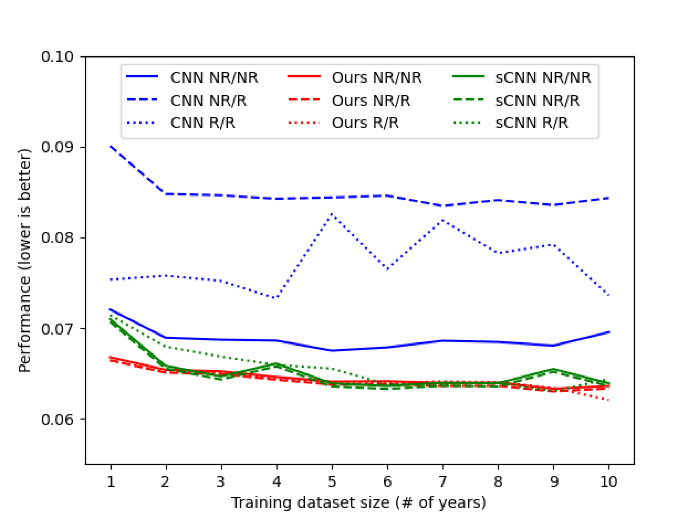
(c) Autoencoder compression on wind data.

Figure 3: Comparison in performance on the test dataset (2022, 2023) between a convolutional UNet (CNN), our implementation of spherical CNN network (sCNN) , and our proposed architecture (Ours), trained on a variable number of years in the training set (years from 2000 to 2009). Our proposed architecture generalizes to unseen rotations even without data augmentation. Increasing the size of the training dataset does not improve the performance of a classic CNN on rotated test samples if data augmentation has not been used during training.

5 Conclusions

Although just a proof of concept, our proposed architecture employing smoothing operators seems to offer a viable alternative to spherical CNNs, trading computational performance for expressivity and accuracy.

In particular, our proposed architecture, which applies a smoothing operator after a non-linearity, consistently outperforms architectures restricting the weights of the convolutions and employing only non-linearities that are signal-equivariant (spherical CNN).

Although in the wind-to-wind prediction, a conventional CNN achieves slightly better performance when rotational data augmentation is used for training, our model outperforms a conventional CNN in the task of temperature-to-wind, where two types of signal-equivariance come into play, even if the CNN is trained using rotational data augmentation.

Impact Statement

This paper presents work whose goal is to advance the field of Machine Learning. There are many potential societal consequences of our work, none of which we feel must be specifically highlighted here.

Appendix A Differential tensors on homogeneous spaces

A.1 Reductive homogeneous spaces and tensors

We want to consider the case where our manifold is a reductive homogeneous space, see e.g. Chapter 5.6 in [23]. Let $G$ be a connected Lie Group with a transitive action on a manifold $M$, making the latter a homogeneous space. If $H=G_{p_{0}}$ is the subgroup of $G$ fixing an arbitrary point $p_{0}\in G$, then we can identify $M$ with the quotient $G/H$ and define a submersion $\pi:G\to M$ by $\pi(g)=g\cdot p_{0}$. Let $\mathfrak{h}$ and $\mathfrak{g}$ be the Lie algebras of $H$ and $G$ respectively. The kernel $\ker\pi_{*}$ of the differential of $\pi:G\to M$ is then given by left translation of $\mathfrak{h}$. We assume that $M$ is a reductive homogeneous space, meaning that we assume that there is a decomposition $\mathfrak{g}=\mathfrak{m}\oplus\mathfrak{h}$, such that $\operatorname{Ad}(H)\mathfrak{m}\subseteq\mathfrak{m}$. It follows that we can consider $\rho(h)X=\operatorname{Ad}(h)X$, $h\in G$, $X\in\mathfrak{m}$ as a representation of $H$ on $\mathfrak{m}$. Furthermore, since $\pi_{*}|_{g\cdot\mathfrak{m}}:g\cdot\mathfrak{m}\to T_{\pi(g)}M$ is a bijective map, any vector field $\xi$ on $M$ can uniquely be described by a function $\boldsymbol{\xi}:G\to\mathfrak{m}$ satisfying

$$\pi_{*}(g\cdot\boldsymbol{\xi}(g))=\xi(\pi(g)),\qquad\text{for any $g\in G$.}$$

Observe that by definition

$$\boldsymbol{\xi}(g\cdot h^{-1})=\rho(h)\boldsymbol{\xi}(g),\qquad g\in G,h\in H,$$

and conversely, any such equivariant function corresponds to a vector field. In a similar way, any $\binom{i}{j}$-tensor $\tau$ on $M$ can be uniquely represented by a $\rho$-equivariant function $\boldsymbol{\tau}:G\to\mathfrak{m}^{*,\otimes i}\otimes\mathfrak{m}^{\otimes j}$ which is called associated to $\tau$. In other words, there exists a unique correspondence between differential tensors on $M$ and equivariant functions $\boldsymbol{\tau}:G\to\mathfrak{m}^{*,\otimes i}\otimes\mathfrak{m}^{\otimes j}$.

A.2 Associated maps on the sphere

We can see the sphere $S^{2}$ as a reductive homogeneous space of the group $\operatorname{SO}(3)$, of $3\times 3$ orthogonal matrices with determinant 1. Such matrices can be written as $A=(A_{1},A_{2},A_{3})$, where the listed columns form a positively oriented orthonormal basis of $\mathbb{R}^{3}$. The Lie algebra $\operatorname{\mathfrak{so}}(3)$ of $\operatorname{SO}(3)$ is spanned by matrices

$$X=\begin{pmatrix}0&0&0\\ 0&0&-1\\ 0&1&0\end{pmatrix}\qquad Y=\begin{pmatrix}0&0&1\\ 0&0&0\\ -1&0&0\end{pmatrix}\qquad Z=\begin{pmatrix}0&-1&0\\ 1&0&0\\ 0&0&0\end{pmatrix},$$

corresponding to infinitesimal rotations around the $x$, $y$ and $z$-axis respectively. With a slight abuse of notation, for $\theta\in\mathbb{R}$, we will also use $Z(\theta)=e^{\theta Z}$ for the rotation matrices themselves and define $X(\theta)$ and $Y(\theta)$ similarly.

We consider the sphere $S^{2}\subseteq\mathbb{R}^{3}$ of 3d-unit vectors. We then have a transitive action by $\operatorname{SO}(3)$ on $S^{2}$ since $Ap$ is a unit vector whenever $p$ is a unit vector. Define a projection $\pi:\operatorname{SO}(3)\to S^{2}$ by $\pi(A)=Ae_{z}=A_{3}$, where the matrix $A$ has columns $(A_{1},A_{2},A_{3})$ and where $e_{z}$ is the unit vector in the $z$-direction. Observe that $\pi(AZ(\theta))=\pi(A)$ and so $\pi$ is invariant under the right action of $H=\{Z(\theta)\}_{\theta\in\mathbb{R}}$. The Lie algebra of $H$ is $\mathfrak{h}=\operatorname{span}\{Z\}$, while $\mathfrak{m}=\operatorname{span}\{X,Y\}$ is an invariant complement, which we can identify with the complex numbers $\mathbb{C}$ with $H$ acting by rotation.

Example A.1 (Functions).

If $f:S^{2}\to\mathbb{R}$ is a real function, the associated function is $\mathbf{f}=f\circ\pi$. Any such function satisfies invariance condition $\mathbf{f}(AZ(\theta))=\mathbf{f}(A)$ for $A\in\operatorname{SO}(3)$, $\theta\in\mathbb{R}$. Conversely, for any such $H$-invariant function $\mathbf{f}:\operatorname{SO}(3)\to\mathbb{R}$ is associated with a function on the sphere defined by

$$f(p)=\textbf{f}\begin{pmatrix}u_{1}&u_{2}&p\end{pmatrix}$$

where $u_{1}$, $u_{2}$ are any unit vectors such that $u_{1}\times u_{2}=p$.

Example A.2 (Vector fields).

Let $\xi$ be a vector field on $S^{2}$. If $A=(A_{1},A_{2},A_{3})$ and $\pi(A)=A_{3}$, then by definition $A_{1},A_{2}$ is an othonormal basis of $T_{A_{3}}S^{2}$. We can hence associate $\xi$ with the function $\boldsymbol{\xi}:\operatorname{SO}(3)\to\mathbb{C}$ defined by

$$\boldsymbol{\xi}(A)=\langle A_{1},\xi(A_{3})\rangle+i\langle A_{2},\xi(A_{3})\rangle.$$

The associated function satisfies equivariance condition

$$\boldsymbol{\xi}(A\cdot Z(\theta))=e^{-i\theta}\boldsymbol{\xi}(A),\qquad A\in\operatorname{SO}(3),\quad\theta\in\mathbb{R}.$$

Conversely, any such equivariant map $\boldsymbol{\xi}:\operatorname{SO}(3)\to\mathbb{C}$ corresponds to a vector field defined by

$$\xi(p)=A\begin{pmatrix}\operatorname{Re}(\boldsymbol{\xi}(A))\\ \operatorname{Im}(\boldsymbol{\xi}(A))\\ 0\end{pmatrix},\qquad p=A_{3}.$$

Example A.3 (Symmetric tensors).

Let $\Sigma$ be a symmetric $\binom{l}{0}$-tensor on $S^{2}$. Let $\mathbb{V}_{l}$ be the space of real-valued polynomials of homogeneous degree $l$ in the variables $x$ and $y$. Then we can describe the tensor $\Sigma$ as a map ${\boldsymbol{\Sigma}}:\operatorname{SO}(M)\to\mathbb{V}_{l}$ with

$${\boldsymbol{\Sigma}}(A)(x,y)=\Sigma(xA_{1}+yA_{2},\dots,xA_{1}+yA_{2}).$$

If we use complex notation $z=x+iy$, then we have equivariance conditions

$${\boldsymbol{\Sigma}}(A\cdot Z(-\theta))(z)={\boldsymbol{\Sigma}}(A)(e^{-i\theta}z),$$

which uniquely define functions associated with symmetric tensors. If we look at coefficients, which for $l$ even is

$${\boldsymbol{\Sigma}}(A)(z)=c_{0}(A)|z|^{l}+\sum_{m=1}^{l/2}\left(c_{2m}(A)z^{l/2+m}\bar{z}^{l/2-m}+\bar{c}_{2m}(A)z^{l/2-m}\bar{z}^{l/2+m}\right),$$

and for $l$ odd

$${\boldsymbol{\Sigma}}(A)(z)=\sum_{m=0}^{(l-1)/2}\left(c_{2m+1}(A)z^{(l+1)/2+m}\bar{z}^{(l-1)/2-m}+\bar{c}_{2m+1}(A)z^{(l-1)/2-m}\bar{z}^{(l+1)/2+m}\right),$$

where $c_{0}$ is real, and $c_{m}(A\cdot Z(-\theta))=e^{-im\theta}c_{m}(A)$.

Appendix B Fourier Analysis and convolutions

B.1 Fourier transform in Euler angles

We can decompose any matrix in $\operatorname{SO}(3)$ as

$$A=Z(\alpha)Y(\beta)Z(\gamma),\qquad 0\leq\alpha,\gamma\leq 2\pi,\quad 0\leq\beta\leq\pi,$$

called the Euler $ZYZ$-representation, see e.g. [24] or Remark B.3 for explicit formula. We note that

$$\pi(Z(\alpha)Y(\beta)Z(\gamma))=p(\alpha,\beta),$$

where $p(\alpha,\beta)$ is the point on the sphere with longitude $\alpha$ and latitude $\beta$. In terms of the $ZYZ$-representation, the unit Haar measure $\mu$ on $\operatorname{SO}(3)$ is given by

$$d\mu=\frac{1}{8\pi^{2}}\sin\beta d\alpha d\beta d\gamma.$$ (B.1)

We have the corresponding $L^{2}$-inner product of signals given by $\langle x,y\rangle_{L^{2}}=\int_{\operatorname{SO}(3)}x\bar{y}\,d\mu$. Consider the space $\mathcal{X}=L^{2}(\operatorname{SO}(3),\mathbb{C})$ of complex-valued square-integrable functions. We define a left and a right action of $\operatorname{SO}(3)$ on $\mathcal{X}$ by $(\ell_{B}x)(A)=x(B^{-1}A)$ and $(r_{B}x)(A)=x(A\cdot B^{-1})$. Consider the subspace $\mathcal{X}_{n}\subseteq\mathcal{X}$ of functions satisfying $(r_{Z(\theta)}x)=e^{in\theta}x$.

In order to discribe the $L^{2}$-space on $\operatorname{SO}(3)$, we will need to describe all its irreducible unitary representations. We follow e.g. [8], Appendix in [12], [10], [21] and [14] in this section. Consider unitary representations $D^{l}:\operatorname{SO}(3)\to U(2l+1)$, $l=0,1,\dots$. To describe these representations, we consider $(2l+1)\times(2l+1)$-matrices, with entries indexed from $-l$ to $l$, defined by

$$\Lambda^{l}=\operatorname{diag}\{m\}_{-l\leq m\leq l},\qquad Q^{l}=(q_{m}^{l}\delta_{m+1,n})_{-l\leq m,n\leq l},\qquad q_{n}^{l}=\sqrt{(l-n)(l+n+1)}.$$

The representation $D^{l}$ is then defined by properties $D^{l}(AB)=D^{l}(A)D^{l}(B)$ and by

$$D^{l}(Z(\alpha))=e^{-i\alpha\Lambda^{l}},\qquad D^{l}(Y(\beta))=d^{l}(\beta):=e^{\beta(Q^{l}-(Q^{l})^{\top})}.$$

Explicitly, the matrix entries are then given by

$$D^{l}_{m,n}(Z(\alpha)Y(\beta)Z(\gamma))=e^{-im\alpha-in\gamma}d_{m,n}^{l}(\beta),$$

where $d^{l}$ is a real, orthogonal matrix. Observe that $r_{Z(\theta)}D_{m,n}^{l}=e^{in\theta}D_{m,n}^{l}$. We also have orthogonality relations

$$\langle D_{m,n}^{l},D_{b,c}^{a}\rangle_{L^{2}}=\frac{1}{2l+1}\delta_{l,a}\delta_{m,b}\delta_{n,c}.$$

Consider the Fourier expansion $x=\sum_{I}\hat{x}_{-m,-n}^{l}D_{m,n}^{l}$. We use the numbering convention such that the Fourier coefficient $\hat{x}_{m,n}^{l}$ corresponds to terms with $e^{im\alpha+in\gamma}d_{-m,-n}^{l}$, in order to have better correspondence with the usual Fourier transform for periodic functions. We can take advantage of the identity

$$Y(\beta)=Z(-\pi/2)Y(-\pi/2)Z(\beta)Y(\pi/2)Z(\pi/2),$$

to obtain a diagonalization of $d^{l}$. If $C^{l}=D^{l}(Z(\pi/2))=\operatorname{diag}\{i^{-m}\}_{-l\leq m\leq l}$ and $\Delta^{l}=D^{l}(Y(\pi/2))=d^{l}(\pi/2)$, then

$$d^{l}(\beta) =C^{l,*}\Delta^{l,*}e^{-i\beta\Lambda^{l}}\Delta^{l}C^{l}=C^{l,*}\Delta^{l,*}\operatorname{diag}\{e^{-im\beta}\}_{-l\leq m\leq l}\Delta^{l}C^{l}$$

$$=C^{l}\Delta^{l,*}e^{i\beta\Lambda^{l}}\Delta^{l}C^{l,*}=C^{l}\Delta^{l,*}\operatorname{diag}\{e^{im\beta}\}_{-l\leq m\leq l}\Delta^{l}C^{l,*},$$

where we have used that $d^{l}$ is real. Explicitly,

$$d^{l}_{m,n}(\beta)=i^{n-m}\sum_{s=-l}^{l}\Delta_{s,m}^{l}\Delta_{s,n}^{l}e^{is\beta}=i^{m-n}\sum_{s=-l}^{l}\Delta_{s,m}^{l}\Delta_{s,n}^{l}e^{-is\beta}.$$

We present the following way of computing the Fourier transform and the inverse Fourier transform on $\operatorname{SO}(3)$, by using the usual Fast Fourier Transform and its inverse.

Lemma B.1.

Let $Y(\beta)$ denote the matrix corresponding to positive rotation around the $y$-axis by an angle $\beta$. Define a matrix $\Delta^{l}=D^{l}(Y(\frac{\pi}{2}))$.

1. For any $x\in\mathcal{X}$, define a periodic function $x^{exp}:\mathbb{R}^{3}/(2\pi\mathbb{Z})^{3}\to\mathbb{C}$

   $$x^{exp}(\alpha,\beta,\gamma)=\left\{\begin{array}[]{cc}x(Z(\alpha)Y(\beta)Z(\gamma))\cdot\sin\beta&\text{if $0\leq\beta\leq\pi$,}\\ 0&\text{if $\pi<\beta<2\pi$,}\end{array}\right.$$

   and write $x^{ext}=\sum_{m,s,n=-\infty}^{\infty}\hat{x}_{m,s,n}^{ext}e^{i(m\alpha+s\beta+n\gamma)}$ for its (usual) Fourier coefficients. Then

   $$\hat{x}_{m,n}^{l}=(-1)^{m+n}i^{m-n}\pi\cdot(2l+1)\sum_{s=-l}^{l}\Delta_{s,m}^{l}\Delta_{s,n}^{l}x^{ext}_{m,s,n}.$$

2. Conversely, if $\mathscr{F}(x)=(\hat{x}_{m,n}^{l})_{I}$ are Fourier coefficients, define a $[0,2\pi]^{3}$-periodic function $X$ by

   $$X(\alpha,\beta,\gamma) =\sum_{m,n,s=-\infty}^{\infty}(-1)^{m+n}i^{n-m}\left(\sum_{l=\max\{|m|,|s|,|n|\}}^{\infty}\hat{x}_{m,n}^{l}\Delta^{l}_{s,m}\Delta^{l}_{s,n}\right)e^{im\alpha+is\beta+in\gamma},$$

   then

   $$X(\alpha,\beta,\gamma)=x(Z(\alpha)Y(\beta)Z(\beta)),\qquad 0\leq\alpha,\gamma\leq 2\pi,0\leq\beta\leq\pi.$$

Proof.

We observe that

$$\frac{1}{2l+1}\hat{x}^{l}_{m,n}=\langle x,D_{-m,-n}^{l}\rangle_{L^{2}}$$

$$=\frac{1}{8\pi^{2}}\int_{0}^{2\pi}\int_{0}^{2\pi}\int_{0}^{\pi}\sum_{s=-l}^{l}i^{m-n}\Delta_{-s,-m}^{l}\Delta_{-s,-n}^{l}xe^{-i(m\alpha+n\gamma+s\beta)}\sin\beta d\beta d\gamma d\alpha$$

$$=\frac{1}{8\pi^{2}}\sum_{s=-l}^{l}i^{m-n}\Delta_{-s,-m}^{l}\Delta_{-s,-n}^{l}\int_{[0,2\pi]^{3}}x^{ext}e^{-i(m\alpha+n\gamma+s\beta)}d\beta d\gamma d\alpha$$

$$=i^{m-n}\pi\sum_{s=-l}^{l}\Delta_{-s,-m}^{l}\Delta_{-s,-n}^{l}x^{ext}_{m,s,n}=(-1)^{m+n}i^{m-n}\pi\sum_{s=-l}^{l}\Delta_{s,m}^{l}\Delta_{s,n}^{l}x^{ext}_{m,s,n},$$

where we have used that $\Delta_{-s,-m}^{l}=(-1)^{s-m}\Delta_{s,m}^{l}$.

Conversely, since

$$x =\sum_{I}\hat{x}_{m,n}^{l}D_{-m,-n}^{l}$$

$$=\sum_{m,n,s=-\infty}^{\infty}i^{n-m}\left(\sum_{l=\max\{|m|,|s|,|n|\}}^{\infty}\hat{x}_{m,n}^{l}\Delta^{l}_{-s,-m}\Delta^{l}_{-s,-n}\right)e^{im\alpha+is\beta+in\gamma}$$

$$=\sum_{m,n,s=-\infty}^{\infty}(-1)^{m+n}i^{n-m}\left(\sum_{l=\max\{|m|,|s|,|n|\}}^{\infty}\hat{x}_{m,n}^{l}\Delta^{l}_{s,m}\Delta^{l}_{s,n}\right)e^{im\alpha+is\beta+in\gamma},$$

we obtain the opposite transformation. ∎

Remark B.2 (Further simplifications).

Since we are developing our method for Fourier transforms for left and right covariances with a filter $\psi$ acting as the (complex) weights in a neural net, we can introduce further simplifications. Including $(2l+1)\cdot\pi$ into the weights, we could just use $\mathbf{R}_{m,s,n}^{l}=(-i)^{m-n}\Delta_{s,m}\Delta_{s,m}$ and

$$\tilde{x}_{m,n}^{l} =\sum_{s=-l}^{l}\mathbf{R}^{l}_{m,s,n}x^{ext}_{m,s,n}.$$

$$X(\alpha,\beta,\gamma) =\sum_{m,n,s=-\infty}^{\infty}\left(\sum_{l=\max\{|m|,|s|,|n|\}}^{\infty}\overline{\mathbf{R}^{l}_{m,s,n}}\tilde{x}_{m,n}^{l}\right)e^{im\alpha+is\beta+in\gamma},$$

If $x_{m,s,n}^{ext}$ only is non-zero for one value of $n$, such as $n=0$ or $n=1$ in our case, then by using a combination of redefining weights and cancellation of constants when taking FFT and then the inverse, we can just use $\mathbf{R}_{m,s,n}^{l}=\Delta_{s,m}\Delta_{s,m}$.

Remark B.3.

Any Euler’s angles decomposition can be explicitly written in terms of $\alpha,\beta,\gamma$ as

$$Z(\alpha)Y(\beta)Z(\gamma)=\begin{pmatrix}\cos(\alpha)\cos(\beta)\cos(\gamma)-\sin(\alpha)\sin(\gamma)&-\cos(\gamma)\sin(\alpha)-\cos(\alpha)\cos(\beta)\sin(\gamma)&\cos(\alpha)\sin(\beta)\\ \cos(\alpha)\sin(\gamma)+\cos(\beta)\cos(\gamma)\sin(\alpha)&\cos(\alpha)\cos(\gamma)-\cos(\beta)\sin(\alpha)\sin(\gamma)&\sin(\alpha)\sin(\beta)\\ -\cos(\gamma)\sin(\beta)&\sin(\beta)\sin(\gamma)&\cos(\beta)\end{pmatrix}.$$

B.2 Convolutions

We will use an approach similar to [5], using conventions in [17]. See also Section 5.4 in [11]. Let $G$ be a compact Lie group which we will assume is unimodular, meaning that its left and right Haar measure coincide. Introduce left and right action on signals by

$$\ell_{g}(x)(h)=x(g^{-1}\cdot h),\qquad r_{g}(x)(h)=x(h\cdot g^{-1}),\qquad g,h\in G,x\in\mathcal{X}(G),$$

where $\mathcal{X}(G)$ are real or complex valued $L^{2}$ functions on $G$. We define the group convolution $x*_{G}y$ as the signal $x*_{G}y(g)=\int_{G}x(h)\overline{y(h^{-1}g)}\,d\mu(h)$. We also introduce left and right covariance defined by

$$x*_{\ell}y(g)=\langle x,\ell_{g}y\rangle_{L^{2}}=\langle\ell_{g^{-1}}x,y\rangle_{L^{2}},\qquad x*_{r}y(g)=\langle x,r_{g}y\rangle_{L^{2}}.$$

related to the convolutions by $x*_{\ell}y=x*_{G}y_{-1}$ and $x*_{r}y=\overline{y_{-1}*_{G}x}$, where $y_{-1}(g)=y(g^{-1})$. We observe equivariance relations that $(\ell_{g}x)*_{\ell}y=\ell_{g}(x*_{\ell}y)$, $(r_{g}x)*_{r}y=r_{g}(x*_{r}y)$. Next, if $x\in\mathcal{X}(G,\mathcal{W})$ is a signal taking values in a real or complex vector space $\mathcal{W}$, and if $\psi\in\mathcal{X}(G)$ is a respectively real or complex valued signal, then both $x*_{\ell}\psi$ and $x*_{r}\psi$ make sense as $\mathcal{W}$-valued functions. Assume that there is a representation $\rho$ of a closed subgroup $H\subseteq G$ on $\mathcal{W}$. If $x$ satisfies $r_{h}x=\rho(h^{-1})x$, we then verify that $r_{h}x*_{r}\psi=\rho(h)x*_{r}\psi$ satisfies the same equivariance property, with a similar relation holding for left covariance.

For the special case of $G=\operatorname{SO}(3)$, we can use the Fourier expansion to write the coefficients these convolutions.

Lemma B.4.

Consider complex-valued signals $x,\psi\in\mathcal{X}=L^{2}(\operatorname{SO}(3),\mathbb{C})$, and write $x=\sum_{I}\hat{x}_{-m,-n}^{l}D_{m,n}^{l}$ and $\psi=\sum_{I}\hat{\psi}_{-m,-n}^{l}D_{m,n}^{l}$. We have Fourier coefficients:

$$\widehat{x*_{\ell}\psi}_{m,n}^{l}=\frac{1}{2l+1}\sum_{s=-l}^{l}\hat{x}_{m,s}^{l}\overline{\hat{\psi}_{n,s}^{l}}.$$

Proof.

Since $D^{l}$ is a representation, we have $D^{l}_{m,n}(AB)=\sum_{s=-l}^{l}D_{m,s}^{l}(A)D_{s,n}^{l}(B)$. It follows that $\ell_{A^{-1}}D_{m,n}^{l}=\sum_{s=-l}^{l}D_{m,s}^{l}(A)D_{s,n}^{l}$. Hence

$$x*_{\ell}\psi(A)=\langle\ell_{A^{-1}}x,\psi\rangle =\sum_{(l,m,n)\in I}\sum_{(a,b,c)\in I}\sum_{s=-l}^{l}\hat{x}_{-m,-n}^{l}\overline{\hat{\psi}_{-b,-c}^{a}}D_{m,s}^{l}(A)\langle D_{s,n}^{l},D_{b,c}^{a}\rangle_{L^{2}}$$

$$=\sum_{(l,m,n)\in I}\frac{1}{2l+1}\sum_{s=-l}^{l}\hat{x}_{-m,s}^{l}\overline{\hat{\psi}_{-n,s}^{l}}D_{m,n}^{l}(A).\qed$$

Similarly, we have $\widehat{y*_{r}\psi}_{m,n}^{l}=\frac{1}{2l+1}\sum_{s=-l}^{l}\hat{x}_{s,n}^{l}\overline{\hat{\psi}_{s,m}^{l}}$. With slight abuse of terminology, we will use convolution for left covariance, as we only use the latter operation in our network layers.

Remark B.5.

Under appropriate bounds, left/right equivariant maps $f:\mathcal{X}(G,\mathcal{W})\to\mathcal{X}(G,\mathcal{W})$ on $L^{2}$ spaces on unimodular Lie groups can be written as left/right covariance with a given filter $\psi\in\mathcal{X}(G)$, see [1] and also [16, 6].

B.3 Interpretation of left- and right-action

Let $\xi$ be a vector field on the sphere $S^{2}$ and let $\boldsymbol{\xi}$ be its associated function on $\operatorname{SO}(3)$. For a fixed $B\in\operatorname{SO}(3)$, consider first the function $\boldsymbol{\xi}_{B}(A)=\boldsymbol{\xi}(B^{-1}A)$. We observe that $\boldsymbol{\xi}_{B}\in\mathcal{X}_{1}$, so it corresponds to a vector field.

$$\xi_{B}(\pi(A)) =\xi_{B}(A_{3})=(\operatorname{Re}\boldsymbol{\xi}(B^{-1}A))A_{1}+(\operatorname{Im}\boldsymbol{\xi}(B^{-1}A))A_{2}$$

$$=\langle B^{-1}A_{1},\xi(B^{-1}A_{3})\rangle A_{1}+\langle B^{-1}A_{2},\xi(B^{-1}A_{3})\rangle A_{2}=B\xi(B^{-1}A).$$

Hence, if we consider the isometry $h(p)=Bp$ of the sphere, then $\xi_{B}$ is the result of the action of this isometry on the vector field

$$\xi_{B}(p)=h_{*}\xi(h^{-1}(p)).$$

Remark B.6.

For $x\in\mathcal{X}_{1}$ the right translation $r_{B}x$ is generally not in $\mathcal{X}_{1}$. However, we observe that $x*_{r}\psi\in\mathcal{X}_{1}$ for any $\psi\in\mathcal{X}$. If we use a rotationally equivariant non-linearity, then we can build a neural network based on layers

$$L(x)=\sigma(x*_{r}\psi).$$

Such a network would map $\mathcal{X}_{1}$ to $\mathcal{X}_{1}$ in a right equivariant way, but our initial experiments with such network also gave inferior results compared to their left invariant counterpart, which is why we did non pursue these beyond their initial testing.

Appendix C Wind data

C.1 Wind directions

Approximate the Earth surface by $S^{2}$ and let $\xi$ be a vector field on $S^{2}$ representing the direction and velocity of the wind. Assume that our data is given in terms of real functions $U(\alpha,\beta)$ and $V(\alpha,\beta)$ determining the signed strength of the wind in the eastward and northward directions respectively, at point $p(\alpha,\beta)\in S^{2}$ where $\beta\neq 0,\pi$. In our setting, $\alpha$ corresponds to the longitude coordinate starting at the Greenwich meridian, while $\beta$ corresponds to the latitude coordinate starting at the north pole. The vector field pointing north outside of the poles is

$$\vec{n}(p)=\frac{1}{\sqrt{1-\langle p,e_{z}\rangle^{2}}}\left(e_{z}-\langle e_{z},p\rangle p\right),$$

which in turn provides us with the east vector in the form $\vec{e}(p)=\vec{n}(p)\times p$. We can write

$$\xi(p(\alpha,\beta))=V(\alpha,\beta)\vec{n}(p(\alpha,\beta))+U(\alpha,\beta)\vec{e}(p(\alpha,\beta))$$

for $p=p(\alpha,\beta)$. Its associated function $\boldsymbol{\xi}(A)=\langle A_{1},\xi(A_{3})\rangle+i\langle A_{2},\xi(A_{3})\rangle$ is computed by

$$\langle A_{j},\vec{n}(A_{3})\rangle=\frac{1}{\sqrt{1-A_{33}^{2}}}A_{3j}\qquad\langle A_{j},\vec{n}(A_{3})\times A_{3}\rangle=\langle A_{3}\times A_{j},\vec{n}(A_{3})\rangle,\qquad j=1,2,$$

we obtain the expression expression

$$\boldsymbol{\xi}(A) =\frac{1}{\sqrt{1-A_{33}^{2}}}\left(U(\alpha,\beta)(A_{32}-iA_{31})+V(\alpha,\beta)(A_{31}+iA_{32})\right)=i(U(\alpha,\beta)+iV(\alpha,\beta))e^{-i\gamma},$$

for Euler angles decomposition $A=Z(\alpha)Y(\beta)Z(\gamma)$.

C.2 Change of coordinate system

When performing a change of coordinates, corresponding to a choice of orthogonal frame for $S^{2}$ we incur interpolation errors due to the non-homogeneous density of the latitude/longitude sampling grid. To minimize unnecessary interpolation errors in the spatial domain we can perform a change of coordinates in the spectral domain. Here we use that if $x\in\mathcal{X}$, $\mathscr{F}(x)=(\hat{x}_{m,n}^{l})_{I}$, then $\mathscr{F}(\ell_{B}x)=(\sum_{s=-l}^{l}\hat{x}_{s,n}b_{s,m})$ with $b_{m,n}^{l}=D_{-m,-n}^{l}(B^{-1})$. For the particular case of $B=Y(\beta)$, we have $b_{m,n}^{l}=d_{-m,-n}^{l}(-\beta)$, thus we can also re-use the precomputed d-matrices that were used for the FFT algorithm.

References

- [1] J. Aronsson. Homogeneous vector bundles and g-equivariant convolutional neural networks. Sampling Theory, Signal Processing, and Data Analysis, 20(2):10, 2022.
- [2] A. Bietti, L. Venturi, and J. Bruna. On the sample complexity of learning under geometric stability. Advances in neural information processing systems, 34:18673–18684, 2021.
- [3] M. M. Bronstein, J. Bruna, T. Cohen, and P. Veličković. Geometric deep learning: Grids, groups, graphs, geodesics, and gauges. arXiv preprint arXiv:2104.13478, 2021.
- [4] T. Cohen. Equivariant convolutional networks. PhD thesis, University of Amsterdam, 2021.
- [5] T. S. Cohen, M. Geiger, J. Köhler, and M. Welling. Spherical cnns. Proceedings of The 6th International Conference on Learning Representations, 2018.
- [6] T. S. Cohen, M. Geiger, and M. Weiler. A general theory of equivariant cnns on homogeneous spaces. Advances in neural information processing systems, 32, 2019.
- [7] C. Esteves, C. Allen-Blanchette, A. Makadia, and K. Daniilidis. Learning equivariant representations with spherical CNNs. In Proceedings of the European Conference on Computer Vision (ECCV), pages 52–68, 2018.
- [8] C. Esteves, A. Makadia, and K. Daniilidis. Spin-weighted spherical cnns. Advances in Neural Information Processing Systems, 33:8614–8625, 2020.
- [9] C. Esteves, J.-J. Slotine, and A. Makadia. Scaling spherical CNNs. 202:9396–9411, 23–29 Jul 2023.
- [10] X. Feng, P. Wang, W. Yang, and G. Jin. High-precision evaluation of wigner’s d matrix by exact diagonalization. Physical Review E, 92(4):043307, 2015.
- [11] G. B. Folland. Harmonic Analysis in Phase Space. Princeton University Press, Princeton, NJ, USA, Mar. 1989.
- [12] J. E. Hansen. Spherical near-field antenna measurements, volume 26. Iet, 1988.
- [13] H. Hersbach, B. Bell, P. Berrisford, S. Hirahara, A. Horányi, J. Muñoz-Sabater, J. Nicolas, C. Peubey, R. Radu, D. Schepers, A. Simmons, C. Soci, S. Abdalla, X. Abellan, G. Balsamo, P. Bechtold, G. Biavati, J. Bidlot, M. Bonavita, G. De Chiara, P. Dahlgren, D. Dee, M. Diamantakis, R. Dragani, J. Flemming, R. Forbes, M. Fuentes, A. Geer, L. Haimberger, S. Healy, R. J. Hogan, E. Hólm, M. Janisková, S. Keeley, P. Laloyaux, P. Lopez, C. Lupu, G. Radnoti, P. de Rosnay, I. Rozum, F. Vamborg, S. Villaume, and J.-N. Thépaut. The ERA5 global reanalysis. Q. J. R. Meteorolog. Soc., 146(730):1999–2049, July 2020.
- [14] K. M. Huffenberger and B. D. Wandelt. Fast and exact spin-s spherical harmonic transforms. The Astrophysical Journal Supplement Series, 189(2):255, 2010.
- [15] A. W. Knapp. Lie groups beyond an introduction, volume 140. Springer, 1996.
- [16] R. Kondor and S. Trivedi. On the generalization of equivariance and convolution in neural networks to the action of compact groups. In International conference on machine learning, pages 2747–2755. PMLR, 2018.
- [17] P. J. Kostelec and D. N. Rockmore. FFTs on the rotation group. Journal of Fourier analysis and applications, 14:145–179, 2008.
- [18] R. Lam, A. Sanchez-Gonzalez, M. Willson, P. Wirnsberger, M. Fortunato, F. Alet, S. Ravuri, T. Ewalds, Z. Eaton-Rosen, W. Hu, et al. Learning skillful medium-range global weather forecasting. Science, 382(6677):1416–1421, 2023.
- [19] J. Milnor. Analytic proofs of the “hairy ball theorem” and the brouwer fixed point theorem. The American Mathematical Monthly, 85(7):521–524, 1978.
- [20] I. Price, A. Sanchez-Gonzalez, F. Alet, T. R. Andersson, A. El-Kadi, D. Masters, T. Ewalds, J. Stott, S. Mohamed, P. Battaglia, et al. Gencast: Diffusion-based ensemble forecasting for medium-range weather. arXiv preprint arXiv:2312.15796, 2023.
- [21] T. Risbo. Fourier transform summation of legendre series and d-functions. Journal of Geodesy, 70:383–396, 1996.
- [22] O. Ronneberger, P. Fischer, and T. Brox. U-Net: Convolutional Networks for Biomedical Image Segmentation. SpringerLink, pages 234–241, Nov. 2015.
- [23] R. W. Sharpe. Differential geometry: Cartan’s generalization of Klein’s Erlangen program, volume 166. Springer Science & Business Media, 2000.
- [24] J. Shen, J. Xu, and P. Zhang. Approximations on so (3) by wigner d-matrix and applications. Journal of Scientific Computing, 74:1706–1724, 2018.