The translation geometry of Pólya’s shires

Abstract.

In his shire theorem, G. Pólya proves that the zeros of iterated derivatives of a meromorphic function in the complex plane accumulate on the union of edges of the Voronoi diagram of the poles of this function. By recasting the local arguments of Pólya into the language of translation surfaces, we prove its generalisation describing the asymptotic distribution of the zeros of a meromorphic function on a compact Riemann surface under the iterations of a linear differential operator $T_{\omega}:f\mapsto\frac{df}{\omega}$ where $\omega$ is a given meromorphic $1$-form. The accumulation set of these zeros is the union of edges of a generalised Voronoi diagram defined by the initial function $f$ together with the singular flat metric on the Riemann surface induced by $\omega$. This result provides the ground for a novel approach to the problem of finding a flat geometric presentation of a translation surface initially defined in terms of algebraic or complex-analytic data.

1. Introduction

1.1. Short historical account

The classical shire theorem of G. Pólya claims that for a meromorphic function $f$ with the set $S$ of its poles, the zeros of its iterated derivatives $f^{(n)}$ accumulate when $n\to+\infty$ along the edges of the Voronoi diagram associated with $S$, see [9]. An illustration of this famous result is shown in Figure 1.

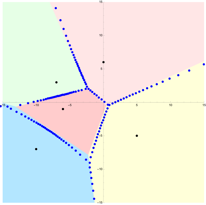
Figure 1. The Voronoi diagram determined by the five poles (black dots) of a rational function $f$, together with the zeros of $f^{(20)}$ in blue dots.

Several prominent mathematicians including N. Wiener, E. Hille, and R. P. Boas have continued Pólya’s line of study soon after the publication of the latter theorem, see references in  [17]. Over the years a number of articles extending and generalising the original result has appeared, see e.g. [5, 6, 7, 18, 19, 21].

More recent publications have concentrated on the weak limits of the root-counting measures for the zeros of $f^{(n)}$. In particular, Ch. Hägg and R. Bøgvad obtained a measure-theoretic refinement of Pólya’s shire theorem for rational functions, see [2]. Using currents they also proved a similar result for Voronoi diagrams associated with generic hyperplane arrangements in $\mathbb{C}^{m}$.

Later Ch. Hägg extended the main result of [2] by considering meromorphic functions of the form $f=Re^{U}$ where $R$ is a rational function with at least $2$ distinct poles and $U$ is a non-constant polynomial, see [8]. The class of such functions coincides with the class of meromorphic functions which are quotients of two entire functions of finite order, each having a finite number of zeros, see [22].

In  [11], V. Keo extended the results of  [2] and  [8] by studying a particular meromorphic function of a different type, namely, $f(z)=1/\left(1-e^{z}\right)$, which has an infinite number of poles and whose iterated derivatives are related to the Eulerian polynomials. In addition, he considered iterations of rational functions under the action of differential operators of the form $\mathcal{D}=g(z)\dfrac{\partial}{\partial z}$, where $g(z)$ is a polynomial in $z$, and studied in details the differential operator $z\dfrac{\partial}{\partial z}$, as well as formulated some conjectures. These cases are closely related to the topic of the present paper.

Finally, in [25], M. Weiss provided a generalisation of Pólya’s classical theorem to automorphic functions in the half-plane.

1.2. Our set-up

There are (at least) two natural ways to generalise the geometry of the complex plane to surfaces of higher genus such as:

• hyperbolic surfaces (the metric still has constant curvature, but it is no longer flat);

• translation surfaces (the metric is still flat, but it has conical singularities).

Below we generalise Pólya’s shire theorem to the case of meromorphic functions on compact Riemann surfaces equipped with a flat metric with conical singularities and study a class of linear differential operators corresponding to the complex-analytic data defining a translation structure, i.e. we use the second of the above generalisations. (For the background on translation surfaces see [28]).

Namely, let $X$ be a compact Riemann surface with a fixed meromorphic $1$-form $\omega$. We associate to the pair $(X,\omega)$ the linear differential operator $T_{\omega}$ acting on meromorphic functions on $X$ as

$$T_{\omega}:f\mapsto\frac{df}{\omega}.$$ (1.1)

Now given a meromorphic function $f$ on $X$, we are interested in the asymptotic of zeros for the sequence $(f_{n})_{n\in\mathbb{N}}$ of meromorphic functions defined inductively as

$$f_{0}=f,~f_{n+1}=T_{\omega}(f_{n})=T_{\omega}^{n+1}(f),~n\geq 1.$$

Definition 1.1.

For a meromorphic function $f$ on a Riemann surface $X$ and any operator $T$ acting on the space of meromorphic functions, define the limit set $\mathcal{L}(T,f)\subseteq X$ as the set of points $z\in X$ such that any open neighbourhood of $z$ in $X$ contains a zero of $T^{n}(f)$ for infinitely many $n$.

In the classical shire theorem, the limit set coincides with the Voronoi diagram in $\mathbb{C}$ associated with the set of poles of a meromorphic function. In our generalised settings, the Voronoi diagram of a meromorphic function on a Riemann surface is defined with respect to the so-called principal polar locus and the singular flat metric induced by the translation structure on the surface.

Definition 1.2.

Consider a (compact) Riemann surface $X$ with a meromorphic $1$-form $\omega$. Given a point $z_{0}\in X$ which is not a pole of $\omega$, we say that a meromorphic function $f$ is locally factorised by a primitive of $\omega$ having no pole at $z_{0}$ if there exist:

• a neighbourhood $U$ of $z_{0}$ in $X$,

• a holomorphic function $\phi$ defined on $U$;

• a holomorphic function $g$ defined on a neighbourhood of $\phi(z_{0})$ in $\mathbb{C}$

such that $\omega=d\phi$ and $f=g\circ\phi$ in $U$.

Below by a non-zero meromorphic $1$-form we always mean a $1$-form not vanishing identically on the underlying Riemann surface.

Definition 1.3.

Consider a non-zero meromorphic $1$-form $\omega$ and a fixed meromorphic function $f$ on a compact Riemann surface $X$. The principal polar locus $\mathcal{PPL}(\omega,f)$ of the pair $(\omega,f)$ is the subset of $X$ containing:

• the poles of $f$ that are not poles of $\omega$;

• the zeros of $\omega$ at which $f$ is not locally factorised by a primitive of $\omega$ (see Definition 1.2).

Remark 1.4.

In the original shire theorem, the Riemann surface is the extended complex plane $\mathbb{C}P^{1}=\mathbb{C}\cup\{{\infty\}}$, $\omega=dz$ and $\mathcal{PPL}(\omega,f)$ is the set of the affine poles of $f$ (i.e. poles different from $\infty$).

The main result of our paper is as follows.

Theorem 1.5.

Consider a non-zero meromorphic $1$-form $\omega$ on a compact Riemann surface $X$, its associated differential operator $T_{\omega}$ and any meromorphic function $f$ on $X$ such that $\mathcal{PPL}(\omega,f)\neq\emptyset$. Then the following two facts are valid.

(i) The limit set $\mathcal{L}(T_{\omega},f)$ is the union of:

• the Voronoi diagram $\mathcal{V}_{\omega,f}$ defined by $\mathcal{PPL}(\omega,f)$ (see Definition 2.10 below);

• the poles of $\omega$ of order at least two;

• the simple poles of $\omega$ that are not poles of $f$.

(ii) The asymptotic root-counting measure of the sequence $(T_{\omega}^{n}(f))_{n\in\mathbb{N}}$ is given by

$$\frac{\mu_{\omega,f}}{A}+\frac{1}{A}\sum\limits_{p\in\mathcal{P}}(d_{p}-1)\delta_{p},$$

where $\mu_{\omega,f}$ is the Cauchy measure of the Voronoi diagram $\mathcal{V}_{\omega,f}$ (see Definition 2.14 below), $\mathcal{P}$ is the set of poles of $\omega$, and $A=\sum\limits_{z\in\mathcal{PPL}(\omega,f)}(a_{z}+1)$ where $z$ is a zero of $\omega$ of order $a_{z}$ and $p\in\mathcal{P}$ is a pole of $\omega$ of order $d_{p}$.

Remark 1.6.

In Polya’s original setup Theorem 1.5 only covers the case of meromorphic functions on $\mathbb{C}P^{1}$, i.e., rational functions. It does not apply to meromorphic functions in $\mathbb{C}$ which have an essential singularity at $\infty$. But following our proof, one might extend Theorem 1.5 to the case of meromorphic functions with possibly essential singularities at any of the poles of $\omega$. We describe this extension briefly in § 7.1.

For a translation surface defined in terms of complex analysis (via a Fuchsian group and a modular form) or algebraic geometry, finding a presentation in terms of flat geometry—specifically, as a polygon with identified edges—is generally a difficult problem. A crucial outcome of Theorem 1.5 is that it determines the incidence structure of the cells of the Voronoi diagram from analytic data. In principle, computing the periods of the relative homology classes of arcs dual to the edges of this diagram is sufficient to construct a flat model. We discuss this perspective in more detail in § 7.2.

1.3. Organisation of the paper

• In Section 2, we provide background on translation surfaces and structures, and introduce the analytic construction of Voronoi diagrams in this setting.

• In Section 3, we characterise asymptotically zero-free regions in terms of Voronoi diagrams.

• In Section 4, we describe the asymptotic distribution of zeros of $T_{\omega}^{n}f$ on Voronoi edges and prove Theorem 1.5.

• In Section 5, we generalise previous results of Prather-Shaw [19] on sequences of derivatives of algebraic functions using the approach of the present paper.

• In Section 6, we describe the limit sets for a number of examples.

• In Section 7, we outline several areas of application for the obtained results, as well as potential generalisations.

Acknowledgements. The second author wants to acknowledge the financial support of his research provided by the Swedish Research Council grant 2021-04900. He is sincerely grateful to Beijing Institute for Mathematical Sciences and Applications for the hospitality in Fall 2023 where the major part of this research has been carried out. Research by the third author is supported by the Beijing Natural Science Foundation IS23005. The authors want to thank Vincent Delecroix, Yi Huang, Pavel Kurasov, Aud Lundholm, and Dmitry Novikov for their interest, valuable remarks and discussions.

2. Preliminary notions and results

2.1. Growth of the order of poles under iterations of $T_{\omega}$

Notice that unless a function $f$ is very special, one expects it to develop poles at the zeros of $\omega$ under iterative applications of the operator $T_{\omega}$. The following lemma describes this phenomenon explicitly.

Lemma 2.1.

Consider a non-zero meromorphic $1$-form $\omega$ and a meromorphic function $f$ on a Riemann surface $X$. Then for any point $z_{0}\in X$ which is not a pole of $\omega$ the following statements are equivalent:

• no function in the sequence $(f_{n})_{n\in\mathbb{N}}$ has a pole at $z_{0}$;

• $f$ is locally factorised at $z_{0}$ by a primitive of $\omega$ (see Definition 1.2).

Proof.

Up to local biholomorphic change of variable $z$, we can assume that $z_{0}=0$ and that $\omega=z^{m}dz$ for some $m\in\mathbb{N}$. An arbitrary locally defined holomorphic function $f$ can be written as a power series in $z$, i.e.,

$$f(z)=\sum\limits_{k=0}^{+\infty}a_{k}z^{k}.$$

Then $T_{\omega}(f)$ is given by a Laurent series of the form:

$$T_{\omega}(f)=\sum\limits_{k=0}^{+\infty}a_{k}kz^{k-m-1}.$$

It follows immediately that if no function in the sequence $(f_{n})_{n\in N}$ has a pole at $0$, then $a_{k}=0$ for all $k\notin(m+1)\mathbb{Z}$.
Introducing the local primitive $\phi=\frac{z^{m+1}}{m+1}$ of $\omega$, we obtain

$$f(z)=\sum\limits_{k=0}^{+\infty}a_{k(m+1)}(m+1)^{k}\phi^{k}.$$

Therefore, in a neighbourhood of $0$, $f$ factorises as $g\circ\phi$ where $g$ is a holomorphic function given by the above series and well-defined near $0$.

Conversely, for any meromorphic function $f$ which locally factorises as $g\circ\phi$, direct computation proves that for any $k$, we have:

$$T_{\omega}^{k}(f)=g^{(k)}\circ\phi.$$

Therefore no iterate $T_{\omega}^{k}(f)$ of $f$ has a pole at $z_{0}$. ∎

The following statement establishes a dichotomy between the points belonging to the principal polar locus $\mathcal{PPL}(\omega,f)$ and the points outside it (see Definition 1.3). On the principal polar locus, the function $T^{k}_{\omega}(f)$ has poles whose orders grow linearly with $k$ while the sum of orders of the poles outside $\mathcal{PPL}(\omega,f)$ remains bounded. In particular, we obtain that when the sum of orders of poles (and thus the sum of orders of zeros) grows to infinity when $k\to\infty$, the principal polar locus must be non-empty. We prove that the sum of orders of poles has linear growth and provide a formula for the leading coefficient of the latter linear dependence.

Proposition 2.2.

Consider a non-zero meromorphic $1$-form $\omega$ and a meromorphic function $f$ on a compact Riemann surface $X$. Then there is an integer $M>0$ such that:

• for any $k>M$ and any point $p\in\mathcal{PPL}(\omega,f)$, $p$ is a pole of $T_{\omega}^{k}(f)$ of order $\alpha_{p}+k(d_{p}+1)$, where $d_{p}$ is the order of $\omega$ at $p$ and $\alpha_{p}$ is some constant;

• for any $k>M$, the sum of orders of the poles of $T_{\omega}^{k}(f)$ outside $\mathcal{PPL}(\omega,f)$ is constant. All these poles are located at the simple poles of $\omega$.

Proof.

Iterating $T_{\omega}$ we get that for any $k\in\mathbb{N}$, any pole of $T_{\omega}^{k}(f)$ is either a pole of $f$ or a zero of $\omega$. Since $X$ is compact, we have only finitely many such points to examine.
Let us first consider the case of a point $p$ which is a pole of $f$ of order $m$ and a pole of $\omega$ of order $-d_{p}$. Direct computation shows that the function $T_{\omega}^{k}(f)$ has at $p$ either a zero or a pole of order $-m-k(d_{p}+1)$. Therefore, if $p$ is a simple pole of $\omega$, it still remains a pole of $T_{\omega}^{k}(f)$ of order $m$ for any $k\in\mathbb{N}$. On the other hand, if $p$ is a pole of $\omega$ of order at least two, then $T_{\omega}^{k}(f)$ is holomorphic at $p$ provided that $k$ is large enough. In both cases, $p$ does not belong to $\mathcal{PPL}(\omega,f)$.

Now, let us consider the case when $p$ is a zero of $\omega$ and $f$ is locally factorised by a primitive of $\omega$. If $p$ is not a pole of $f$, then Lemma 2.1 proves that $p$ is not a pole of any function in the sequence $(f_{n})_{n\in N}$. Thus, we have shown that after finitely many steps, the sum of orders of the poles of $T_{\omega}^{k}(f)$ outside $\mathcal{PPL}(\omega,f)$ stabilises to the sum of orders of the poles of $f$ coinciding with the simple poles of $\omega$.

Lemma 2.1 implies that for any point $p$ of $\mathcal{PPL}(\omega,f)$, there exists $k_{p}\in\mathbb{N}$ such that $T_{\omega}^{k_{p}}(f)$ has a pole at $p$. Then direct computation proves that the order of the pole increases by $d_{p}+1$ with each application of $T_{\omega}$ which finishes the proof. ∎

Corollary 2.3.

Consider a non-zero meromorphic $1$-form $\omega$ and a meromorphic function $f$ on a compact Riemann surface $X$ such that $\mathcal{PPL}(\omega,f)\neq\emptyset$. For any $z\in\mathcal{PPL}(\omega,f)$, let $a_{z}$ be the order of $\omega$ at $z$.

Then the sum $\mathcal{Z}_{n}$ of orders of the poles of the meromorphic function $T_{\omega}^{n}(f)$ (and therefore the sum of orders of its zeros) grows when $n\rightarrow\infty$ as $\mathcal{Z}_{n}\sim A\cdot n$ where

$$A=\sum\limits_{z\in\mathcal{PPL}(\omega,f)}(a_{z}+1).$$

2.2. Translation structures

Any non-zero meromorphic $1$-form $\omega$ on a (possibly open) Riemann surface $X$ defines on $X$ a geometric structure called translational. Denote by

• $X^{\ast}$ the surface $X$ punctured at the poles of $\omega$;

• $X^{\ast\ast}$ the surface $X$ punctured at the zeros and the poles of $\omega$.

Local primitives of $\omega$ are locally injective on $X^{\ast\ast}$. They form an atlas of local biholomorphisms from $X$ to $\mathbb{C}$. Additionally, since any two local primitives of the same differential $1$-form $\omega$ differ by a constant, transition maps between two distinct charts of the atlas are translations of the complex plane. Therefore, we say that $\omega$ endows the Riemann surface $X$ with a translation structure. The pair $(X,\omega)$ is called a translation surface; see [28] for general background on translation surfaces.

Differential $\omega$ induces a flat metric $|\omega|$ in the following way: for any point $z_{0}\in X^{\ast\ast}$, the distance between $z_{0}$ and any other point $z$ in a small enough neighbourhood of $z_{0}$ is defined as $\lvert\int\limits_{z_{0}}^{z}\omega\rvert$. For example, the standard differential $dz$ endows the complex plane $\mathbb{C}$ with the standard Euclidean metric $|dz|$. Any chart $\phi$ of the translation atlas, i.e. a local primitive of $\omega$, conjugates the standard differential $dz$ in the complex plane with a differential $\omega$ defined on $X$. In other words, we have $\phi^{\ast}dz=\omega$. Thus we can think of a translation surface as formed by pieces of the standard complex plane $\mathbb{C}$ glued together with the help of translations.

In this way the punctured surface $X^{\ast\ast}$ obtains a flat metric $|\omega|$. The latter naturally extends to the zeros of $\omega$ as follows. A neighbourhood of a zero of $\omega$ of order $k$ is mapped (by any local primitive) to the complex plane as a ramified cyclic cover of degree $k+1$. It follows that the flat metric $|\omega|$ extends to such a zero as having a conical singularity of angle $2(k+1)\pi$. Therefore the punctured surface $X^{\ast}$ is a Euclidean surface with conical singularities, see [23].

Remarkably, as soon as a meromorphic differential defined on a compact Riemann surface has poles, the metric structure it defines on the surface punctured at these poles is no longer compact. The following fact is well known (see [3] for a reference on the flat geometry of meromorphic $1$-forms)

Lemma 2.4.

Let $X$ be a compact Riemann surface with a non-zero meromorphic $1$-form $\omega$. Then the punctured surface $X^{\ast}$ is a complete metric space for the singular flat metric $|\omega|$.

Proof.

We have to prove that any Cauchy sequence $(z_{n})_{n\in\mathbb{N}}$ of points in $X^{\ast}$ converges to some limit point in $X^{\ast}$. Since $X^{\ast}$ is locally compact and $\omega$ has finitely many poles, the question reduces to the only case when $(z_{n})_{n\in\mathbb{N}}$ converges in $X$ to some point $z_{\infty}$ which is a pole of $\omega$. We will prove that no such sequence can be a Cauchy sequence in the flat metric $|\omega|$.

Indeed, let $k\in\mathbb{N}^{\ast}$ and $\lambda\in\mathbb{C}$ be the order and the residue of $\omega$ at the pole $z_{\infty}$ respectively. Up to a biholomorphic change of $z$, we can assume that $z_{\infty}=0$ and normalise $\omega$ as $(\frac{\lambda}{z}+\frac{1}{z^{k}})dz$ for $k\geq 2$ and as $\frac{\lambda dz}{z}$ for $k=1$; see Section 2.3 in [3] for the details on the local models of poles in translation surfaces.

Up to a choice of a subsequence, we can assume that the sequence $(z_{n})_{n\in\mathbb{N}}$ belongs to the domain of a unique chart $\phi:z\mapsto\lambda\ln(z)-\frac{1}{(k-1)z^{k-1}}$ if $k\geq 2$ and $\phi:z\mapsto\lambda\ln(z)$ if $k=1$. The fact that this sequence $(z_{n})_{n\in\mathbb{N}}$ is a Cauchy sequence with respect to the metric $|\omega|$ means exactly that the sequence $(\phi(z_{n}))_{n\in\mathbb{N}}$ is a Cauchy sequence in the complex plane and therefore it converges to some point. It is therefore disjoint from any sufficiently small neighbourhood of $z_{\infty}$ when $n\to\infty$ which finishes the proof. ∎

2.3. Voronoi functions

For a meromorphic function $f$ in $\mathbb{C}$, the Voronoi diagram of its set of poles can be defined in terms of maximal embedded disks disjoint from these poles. Voronoi functions play a similar role on translation surfaces.

Definition 2.5.

Consider a compact Riemann surface $X$ with a non-zero meromorphic $1$-form $\omega$ and a meromorphic function $f$ on $X$. Let $z\in X^{\ast}\setminus\mathcal{PPL}(\omega,f)$.

Denote by $\phi$ a local primitive of $\omega$ such that $\phi(z)=0$. The Voronoi function $g_{z}$ is the holomorphic function defined in a neighbourhood of the origin in the complex plane $\mathbb{C}$ and satisfying $g_{z}\circ\phi=f$ (see Definitions 1.2 and 1.3 for the existence and uniqueness of $g_{z}$ if $z$ is a zero of $\omega$).

The critical radius $\rho(z)$ is the radius of convergence of $g_{z}$ at $0$. Immediate computation shows that for any $k\geq 1$, $g_{z}^{(k)}\circ\phi=T_{\omega}^{k}(f)$.

Our next result shows that the behaviour of $g_{z}$ on the boundary of its disk of convergence at $0$ reflects the geometry of the translation surface $(X,\omega)$.

Lemma 2.6.

Consider a compact Riemann surface $X$ with a non-zero meromorphic $1$-form $\omega$ and a meromorphic function $f$. Let $z\in X^{\ast}\setminus\mathcal{PPL}(\omega,f)$, and denote by $\tilde{z}$ some preimage of $z$ in the universal cover $\pi:\tilde{X^{\ast}}\rightarrow X^{\ast}$. Consider the primitive $\tilde{\phi}$ of $\pi^{\ast}\omega$ in $\tilde{X^{\ast}}$ such that $\tilde{\phi}(z)=0$.

Then for any path $\sigma:[0,1]\rightarrow\mathbb{C}$ such that

• $\sigma(0)=0$;

• $|\sigma(s)|<\rho(z)$ for any $s\in[0,1[$;

• $|\sigma(1)|\leq\rho(z)$;

there exists a path $\tilde{\gamma}:[0,1]\rightarrow\tilde{X^{\ast}}$ such that $\tilde{\phi}\circ\tilde{\gamma}=\sigma$. In addition one of the following two statements holds:

1. either $\pi\circ\tilde{\gamma}(1)\notin\mathcal{PPL}(\omega,f)$ and $g_{z}$ extends to $\sigma(1)$ as a holomorphic function;

2. or $\pi\circ\tilde{\gamma}(1)\in\mathcal{PPL}(\omega,f)$ and $g_{z}$ does not extends to $\sigma(1)$ as a holomorphic function. However, it extends in a neighbourhood of $\sigma(1)$ as a convergent Puiseux series.

Proof.

The existence of a path $\tilde{\gamma}:[0,1]\rightarrow\tilde{X^{\ast}}$ satisfying $\tilde{\phi}\circ\tilde{\gamma}=\sigma$ follows from the metric completeness of $(X^{\ast},|\omega|)$ (see Lemma 2.4).

Analytic continuation along the path $\tilde{\gamma}$ proves that the function $g_{z}\circ\tilde{\phi}$ coincides with $f\circ\pi$. (Recall that $\pi$ is the projection of $\tilde{X^{\ast}}$ to $X^{\ast}$).)

We first consider the case when $\pi\circ\tilde{\gamma}(1)\notin\mathcal{PPL}(\omega,f)$. Following Definitions 1.2 and 1.3, there is a neighbourhood of $\pi\circ\tilde{\gamma}(1)$ in $X^{\ast}$ in which $f$ is factorised by $\phi$. Thus $g_{z}$ extends to $\sigma(1)$ as a holomorphic function.

If $\pi\circ\tilde{\gamma}(1)\in\mathcal{PPL}(\omega,f)$ but is not a zero of $\omega$, then $\phi$ is locally injective in a neighbourhood of $\pi\circ\tilde{\gamma}(1)$ and the meromorphic function $f$ can be factorised by $\phi$. Therefore $g_{z}$ extends to $\sigma(1)$ as a pole of a meromorphic function.

In the latter case, $\pi\circ\tilde{\gamma}(1)$ is a zero of $\omega$ of order $k$. Equivalently, $\tilde{\gamma}(1)$ is a critical point of $\tilde{\phi}$ of order $k$. The equation $f\circ\pi=g\circ\tilde{\phi}$ can be locally solved at $\tilde{\gamma}(1)$ if we consider $g$ as a convergent Puiseux series with exponents belonging to $\frac{1}{k+1}\mathbb{Z}$. This provides the correct extension of $g_{z}$ to $\sigma(1)$. The function $g_{z}$ cannot extend to $\sigma(1)$ holomorphically because in this case, $f$ will be locally factorised (see Definition 1.2) by a primitive of $\omega$ and $\tilde{\gamma(1)}$ would not belong to the principal polar locus. ∎

Corollary 2.7.

Consider a compact connected Riemann surface $X$ with a non-zero meromorphic $1$-form $\omega$ and a meromorphic function $f$ on $X$ such that $\mathcal{PPL}(\omega,f)\neq\emptyset$. Then any point $z\in X^{\ast}\setminus\mathcal{PPL}(\omega,f)$ has a finite critical radius $\rho(z)$.

Proof.

We assume by contradiction that $\rho(z)=+\infty$, i.e. that $g_{z}$ is an entire function. Since $X$ is connected and $\mathcal{PPL}(\omega,f)\neq\emptyset$, there is a real-analytic path $\gamma:[0,1]\rightarrow X^{\ast}$ such that $\gamma(0)=0$ and $\gamma(1)=z_{0}$ where $z_{0}\in\mathcal{PPL}(\omega,f)$. The path $\gamma$ lifts to a path $\tilde{\gamma}$ on the universal cover $\tilde{X^{\ast}}$. The path $\tilde{\gamma}$ satisfies the assumptions of Lemma 2.6 and we conclude that $g_{z}$ is not holomorphic at $\tilde{\phi}\circ\tilde{\gamma}(1)$ which is a contradiction. ∎

2.4. Voronoi diagrams

Let us now stratify the translation surface $(X,\omega)$ into cells according to the values of the Voronoi index defined below.

Definition 2.8.

Let $X$ be a compact connected Riemann surface $X$ with a non-zero meromorphic $1$-form $\omega$ and a meromorphic function $f$ such that $\mathcal{PPL}(\omega,f)\neq\emptyset$. For any point $z\in X^{\ast}\setminus\mathcal{PPL}(\omega,f)$, let $g_{z}$ be the Voronoi function of $z$ and let $\rho(z)$ be the critical radius at $z$.

Then the Voronoi index $\nu_{z}$ is the number of points on the circle of radius $\rho(z)$ centered at $0$ at which $g_{z}$ does not extend as a holomorphic function.

Lemma 2.9.

For any point $z\in X^{\ast}\setminus\mathcal{PPL}(\omega,f)$, $\nu_{z}$ is a positive integer.

Proof.

Following Corollary 2.7, the radius $\rho(z)$ of convergence of $g_{z}$ at $0$ is finite and $g_{z}$ fails to extend to a holomorphic function at least at one point of the circle of radius $\rho(z)$. At each of these singular points, $g_{z}$ extends as a Puiseux series converging in some neighbourhood of such a point (see Lemma 2.6). Compactness argument then proves that there can be at most finitely many such points inside the considered circle. ∎

All points in a punctured neighbourhood of a point $z\in\mathcal{PPL}(\omega,f)$ will satisfy $\nu=1$, and we extend the definition by setting $\nu_{z}=1$. Assuming that the principal polar locus is nonempty, the values of the Voronoi index decompose the underlying surface $X$ into:

• the Voronoi cells (for which $\nu=1$);

• the Voronoi edges (for which $\nu=2$);

• the Voronoi vertices (for which $\nu\geq 3$).

Definition 2.10.

Consider a compact Riemann surface $X$ with a non-zero meromorphic $1$-form $\omega$ and a meromorphic function $f$ on $X$ such that $\mathcal{PPL}(\omega,f)\neq\emptyset$. The Voronoi diagram $\mathcal{V}_{\omega,f}$ of pair $(\omega,f)$ is the union of all points $z\in X$ such that $\nu_{z}\geq 2$; i.e. the union of Voronoi edges and vertices.

Proposition 2.11.

Consider a compact Riemann surface $X$ with a non-zero meromorphic $1$-form $\omega$ and a meromorphic function $f$ on $X$ such that $\mathcal{PPL}(\omega,f)\neq\emptyset$. Then $\mathcal{V}_{\omega,f}$ is the union of geodesic segments in the (singular) flat metric $|\omega|$.

Proof.

For any point $z_{0}\in\mathcal{V}_{\omega,f}$ of critical radius $r$ and Voronoi index $\nu$, let us denote by $\alpha_{1},\dots,\alpha_{\nu}$ the points of $\{{t\in\mathbb{C}~|~|t|=r\}}$ where the Voronoi function $g_{z_{0}}$ does not extend as a holomorphic function.

Actually, there exists $\epsilon>0$ such that $g_{z_{0}}$ extends as a holomorphic function to a domain $\mathcal{D}$ formed by the points of the open disk $\{{x\in\mathbb{C}~|~|x|<r+\epsilon\}}$ which do not belong to the cuts $[1,\frac{r+\epsilon}{r}[\alpha_{i}$ for $1\leq i\leq\nu$.

For any two distinct $i,j\in\{{1,\dots,\nu\}}$, let the line $L_{ij}$ be the midline of the segment $[\alpha_{i},\alpha_{j}]$, i.e. the line perpendicular to $[\alpha_{i},\alpha_{j}]$ and passing through its midpoint. Denote by $\mathcal{L}$ the union of all these lines $L_{ij}$ for $1\leq i<j\leq\nu$.

Consider a small neighbourhood $U$ of $z_{0}$ in $X$ in which $\omega$ has a well-defined primitive $\phi$ satisfying the condition $\phi(z_{0})=0$. We can assume that for any $z\in U$, $|\phi(z)|<\delta$ where $\delta<\frac{\epsilon}{2}$. It follows that for any $z\in U$, the disk of convergence of $g_{z}$ in $\phi(z)$ is contained in $\mathcal{D}$, see Figure 2. Moreover, unless $\phi(z)\in\mathcal{L}$, we have $\nu(z)=1$.

In the open set $U$, $\phi^{-1}(\mathcal{L})$ is the union of straight segments in the flat coordinate $\phi$ which finishes the proof. ∎

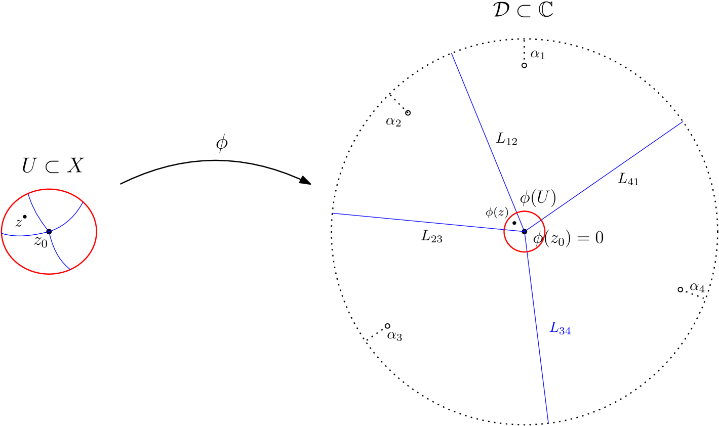
Figure 2. The Voronoi function $g_{z_{0}}$ extends to a holomorphic function in the domain $\mathcal{D}$. The blue lines form the union $\mathcal{L}$ of the midline rays contained in $\mathcal{D}$. The preimage $\phi^{-1}(\mathcal{L})$ is the union of the straight segments with respect to the coordinate $\phi$ in $U$.

Remark 2.12.

Observe that the Voronoi diagrams cannot be defined in purely metric terms, as demonstrated by the following example. Consider $\omega=zdz$ and $f(z)=\frac{1}{z^{2}-1}$. Since $f$ is factorised by a primitive $\phi:z\mapsto\frac{1}{2}z^{2}$ of $\omega$, we have $\mathcal{PPL}(\omega,f)=\{{\pm 1\}}$.

The points equidistant to $1$ and $-1$ (with respect to $|zdz|$) satisfy the equation $\operatorname{Re}(z)=0$. However, since $1$ and $-1$ have the same image under $\phi$, there is no point $z$ in $\mathbb{C}\setminus\{{\pm 1\}}$ such that the corresponding Voronoi function $g_{z}$ has more than one singular point on its critical circle. Therefore the Voronoi diagram is empty and, in particular, it does not coincide with the imaginary axis as a purely metric definition might suggest.

2.5. Cauchy measure of a Voronoi diagram

We shall define the Cauchy measure $\mu_{\omega,f}$ of the Voronoi diagram $\mathcal{V}_{\omega,f}$ by using central angles at points of $\mathcal{PPL}(\omega,f)$,. It is obtained as the pullback of a certain differential form by a local primitive of $\omega$.

Definition 2.13.

Let $A,B$ be two distinct points in the complex plane. Denote by $L_{AB}$ their midline, i.e. the line perpendicular to the segment $[A,B]$ and passing through its middle point. We define the unnormalised Voronoi angular measure $\theta$ on $L_{AB}$ as follows. For any segment $[M,N]$ contained in $L_{AB}$, let $\theta([M,N])$ be the angle at the vertex $A$ of the triangle $AMN$ (see Figure 3). Obviously, $\theta(L_{AB})=\pi$.

We define the normalised Voronoi measure as $\Theta=\frac{1}{\pi}\theta$. It is a probability measure on $L_{AB}$. We note for the later use that the density of $\Theta$ on $L_{AB}$ is given by

$$d\Theta_{AB}(P):=\frac{|A-B|}{2\pi|P-A||P-B|}d\lambda(P),$$

where $d\lambda$ is the Euclidean length on $L_{AB}$.

Figure 3. Illustration of the angular measure $\theta$ on the midline $L_{AB}$ of two points $A$ and $B$ in the plane.

Definition 2.14.

Consider a compact Riemann surface $X$ together with a non-zero meromorphic $1$-form $\omega$ and a meromorphic function $f$ such that $\mathcal{PPL}(\omega,f)\neq\emptyset$.

Then the Cauchy measure $\mu_{\omega,f}$ of the Voronoi diagram $\mathcal{V}_{\omega,f}$ is obtained by the integration of the differential form obtained as the pullback of the differential form $d\Theta_{AB}$ at each point $z$ such that $\nu_{z}=2$, by a local primitive $\phi$ of $\omega$ satisfying $\phi(z)=0$, see Definition 2.13.

Remark 2.15.

Since the principal polar locus contains finitely many points with a finite conical angle at each of them, the Cauchy measure $\mu_{\omega,f}$ of the whole Voronoi diagram is finite. Besides, it is invariant under the rescaling $\omega\mapsto\lambda\omega$ where $\lambda\in\mathbb{C}^{\ast}$.

3. Zero-free regions

In this section, we prove that zeros of iterates of the operator $T_{\omega}$ applied to a meromorphic function $f$ cannot accumulate inside Voronoi cells, i.e. in the complement to the Voronoi diagram $\mathcal{V}_{\omega,f}$.

Proposition 3.1.

Let $X$ be a compact connected Riemann surface $X$ with a non-zero meromorphic $1$-form $\omega$ and a meromorphic function $f$ such that $\mathcal{PPL}(\omega,f)\neq\emptyset$.

Then

$$\lim_{n\to\infty}\dfrac{1}{n}\log\left|\frac{T_{\omega}^{n}f(z)}{n!}\right|=\log\frac{1}{\rho(z)}$$

on every compact subset of the union of the Voronoi cells, i.e., on the open subset $U\subset X^{\ast\ast}$ formed by all points $z$ satisfying $\nu_{z}=1$, (see Definition 2.8). Here $\rho(z)$ is the critical radius of the Voronoi function $g_{z}$, see Definition 2.5.

In particular, for any compact subset $K\subset U$, there is a positive integer $N$ such that for any $n>N$, $T_{\omega}^{n}(f)$ has no zeros in $K$.

Proposition 3.1 will be deduced from a purely analytic lemma about the asymptotics of the coefficients of the Taylor series of a Puiseux series, due to Orlov in [15]. Lemma 3.2 applies a uniform version of his result, see Corollary A.2 below.

Lemma 3.2.

Let $g$ be a holomorphic function on the open centered disk $D(0,R)\subset\mathbb{C}$ of radius $R>0$. Suppose that $g$ can be extended holomorphically to $\partial D(R)$, except at only one point $d$ on the boundary circle $\partial D(R)$ around which it extends as a Puiseux series(with non-integer exponents). Then, there exists $\delta>0$ such that

$$\frac{1}{n}\log\left|\frac{g^{(n)}(x)}{n!}\right|\to\log\frac{1}{|x-d|}$$

uniformly on the closed disk $\overline{D}(0,\delta)$ of radius $\delta$.

Proof.

Suppose that the Puiseux series at $d$ has a leading exponent $m_{0}$, meaning that $B_{m_{0}}(d-x)^{m_{0}}$ is the term with the smallest non-integer or the smallest negative exponent.

By Corollary A.2, there exist $\epsilon,\delta>0$ such that on $\overline{D}(0,\delta)$ one has the asymptotic behavior

$$\frac{g^{(n)}(x)}{n!}=b(n,x)(d-x)^{-n}+O\left((|d-x|(1+\epsilon))^{-n}\right),$$

where

$$b(n,x)=K(x-d)^{m_{0}}n^{-(m_{0}+1)}(M+O(n^{-\frac{1}{M}}|x-d|^{\frac{1}{M}})),$$

with all constants depending only on $g$ and $R$. Then,

$$\left|\frac{g^{(n)}(x)}{n!}\right|=|d-x|^{-n}\left|b(n,x)+O((1+\epsilon)^{-n})\right|.$$ (3.1)

We claim that the expression $\frac{1}{n}\log|b(n,x)+O((1+\epsilon)^{-n})|$ converges as $n\to\infty$ to 0 uniformly on $\overline{D}(0,\delta)$. It suffices to check that $\log|b(n,x)|$ grows at a slower rate than a power of $n$ in $\overline{D}(0,\delta)$. This holds because there exist constants $C_{1},C_{2}$ for which the inequality

$$C_{1}n^{-(m_{0}+1)}\leq|b(n,x)|\leq C_{2}n^{-(m_{0}+1)}$$

holds for all $x$ and sufficiently large $n$. Therefore, taking log of (3.1), dividing by $n$, and taking limits results in

$$\lim\limits_{n\to+\infty}\frac{1}{n}\log\left|\frac{g^{(n)}(x)}{n!}\right|=-\log|x-d|$$

where the convergence is uniform in $\overline{D}(\delta)$ as claimed. ∎

We now prove Proposition 3.1 by applying Lemma 3.2 to the Voronoi function of a point contained in a Voronoi cell.

Proof of Proposition 3.1.

For any $z_{0}\in U$, the Voronoi function $g_{z_{0}}$ converges in the open disk of radius $\rho(z_{0})$ centered at $0$ and extends as a holomorphic function to every point of its boundary circle, except at one point $d$, to a neighbourhood of which $g_{z_{0}}$ extends as a Puiseux series (see Lemma 2.6 and Definition 2.8). Using Lemma 3.2 we then deduce the existence of a neighbourhood $W$ of $0$ in which the sequence of functions ${\frac{1}{n}}\log\left|\frac{g^{(n)}_{z_{0}}(x)}{n!}\right|$ converges to $-\log|x-d|$ uniformly. Therefore, there is a neighbourhood of $z_{0}$ in $X$ in which

$${\frac{1}{n}}\log\left|\frac{T_{\omega}^{n}(f)(z)}{n!}\right|={\frac{1}{n}}\log\left|\frac{g^{(n)}_{z_{0}}(\phi(z))}{n!}\right|$$

converges uniformly to $-\log{\rho(z)}$ where $\rho(z)$ is the radius of convergence of $g_{z}$. The last claim follows immediately. ∎

4. Edges in the limit set

The remaining part of the proof of Theorem 1.5 is an application of certain results of the logarithmic potential theory. We will first show that

$$\lim_{n\to\infty}\dfrac{1}{n}\log\left|\frac{T_{\omega}^{n}f(z)}{n!}\right|=\log\frac{1}{\rho(z)}$$

in the space $L^{1}_{loc}(X^{\ast})$ of locally integrable with respect to the measure $\omega\wedge\overline{\omega}$ functions on $X^{\ast}$. Next introducing the Laplace operator $\Delta_{\omega}$ induced by the flat metric $|\omega|$ on $X^{\ast}$, we prove that (up to normalisation) the Laplacian of $\dfrac{1}{n}\log\left|\frac{T_{\omega}^{n}f(z)}{n!}\right|$ considered as a distribution coincides with the root-counting measure of $T_{\omega}^{n}f(z)$. When $n\to\infty$, the sequence of these Laplacians converges as a distribution or a measure to $\frac{\mu_{\omega,f}}{A\pi}+\frac{1}{A}\sum\limits_{p\in\mathcal{P}}(d_{p}-1)\delta_{p}$. This claim is exactly the second part of Theorem 1.5. After that we will deduce the first part of Theorem 1.5 from this convergence.

4.1. Convergence in $L^{1}_{loc}(X^{\ast})$

Proposition 3.1 shows that $\frac{1}{n}\log\left|\frac{T_{\omega}^{n}f(z)}{n!}\right|$ converges uniformly to $\log\frac{1}{\rho(z)}$ on every compact subset inside the union of the Voronoi cells of $X$, not containing the singularities. Oscillations of $T_{\omega}^{n}f(z)$ near the edges of the Voronoi diagram force us to work with the weaker type of convergence, namely, with the $L^{1}_{loc}$-convergence.

Proposition 4.1.

Let $\omega$ be a meromorphic 1-form and $f$ a meromorphic function on a compact Riemann surface $X$. Assume that $\mathcal{PPL}(\omega,f)\neq\emptyset$. For any $z\in X^{\ast}$, there exists a neighbourhood $U$ of $z$ such that on any compact subset $K\subset U$, one has

$$\lim_{n\to\infty}\int\limits_{K}\bigg{|}\frac{1}{n}\log\big{|}\frac{T_{\omega}^{n}f(z)}{n!}\big{|}-\log\frac{1}{\rho(z)}\bigg{|}\ \omega\wedge\overline{\omega}=0,$$

where $\rho(z)$ is the critical radius of the Voronoi function $g_{z}$.

To do this, we first need to check that $\log\frac{1}{\rho(z)}$ is a locally integrable function.

Lemma 4.2.

In the notation as Proposition 4.1, assuming that $\mathcal{PPL}(\omega,f)\neq\emptyset$, the function $z\mapsto\log\frac{1}{\rho(z)}$ belongs to $L^{1}_{loc}(X^{\ast})$.

Proof.

For any $z_{0}\in X^{\ast}\setminus\mathcal{PPL}(\omega,f)$, consider its Voronoi function $g_{z_{0}}$ and a local primitive $\phi$ of $\omega$ such that $\phi(z_{0})=0$. Let $d_{1},\dots,d_{k}$ be the points of the critical circle where $g_{z_{0}}$ does not extend holomorphically, with $k$ being the Voronoi index of $z_{0}$, see Lemma 2.9. Then, there is a neighbourhood $U$ of $z_{0}$ such that for any $z\in U$, $\rho(z)=\min\limits_{1\leq i\leq k}|\phi(z)-d_{i}|$.

Calculating a simple integral we can show that the function $w\mapsto\log|w-b|$ for some constant $b\in\mathbb{C}$ is locally integrable, in any compact set, possibly containing $b$. It follows that $x\mapsto-\min\limits_{1\leq i\leq k}\log|x-d_{i}|$ is locally integrable in $\mathbb{C}$. We deduce that $z\mapsto\log\frac{1}{\rho(z)}$ is integrable in a small enough neighbourhood of $z_{0}$ in $X^{\ast}$. The claim follows. ∎

Proposition 4.1 follows from Lemma 4.3 below whose proof is postponed until Section 4.2.

Lemma 4.3.

Let $g$ be a holomorphic function on the open centered disk (at 0) $D(\rho)\subset\mathbb{C}$ of radius $\rho>0$. Suppose that $g$ can be extended holomorphically to $\partial D(\rho)$, except for finitely many points $d_{1},\dots,d_{k}$ on the boundary circle $\partial D(\rho)$ where it extends as a Puiseux series. Then, setting

$$M(x)=-\min\limits_{1\leq i\leq k}\log|x-d_{i}|,$$

there exists $\delta>0$ such that

$$\int\limits_{\overline{D}(\delta)}\left|\frac{1}{n}\log\big{|}\frac{g^{(n)}(x)}{n!}\big{|}-M(x)\right|d\lambda\longrightarrow 0$$

where $\overline{D}(\delta)$ is the closed centered disk of radius $\delta$ and $d\lambda$ is the standard Lebesgue measure.

Proof of Proposition 4.1.

For any $z_{0}\in X^{\ast}\setminus\mathcal{PPL}(\omega,f)$, we can apply Lemma 4.3 to the Voronoi function $g_{z_{0}}$. Notice that $\omega\wedge\overline{\omega}=\phi^{\ast}d\lambda$ and $T_{\omega}^{k}(f)=g^{(k)}\circ\phi$. This shows the required convergence to 0 in a compact set not containing $\mathcal{PPL}(\omega,f)$, and it remains to prove that in a small enough neighbourhood of a point $a$ in $\mathcal{PPL}(\omega,f)$, the integral can be made arbitrarily small independent of $n$. We argue as follows. Note that if the statement is true for the derivative $g^{(k)}$ then it is also true for $g$, since $\frac{1}{n}\log\big{(}\frac{(k+n)!}{n!}\big{)}\to 0$ as $n\to\infty$. Hence we take a derivative of our function of sufficiently large order and, in particular, assume that $m_{0}+1\leq-\frac{1}{M}$ in a neighbourhood given by $|z-a|<1$. This allows us to rewrite the asymptotic estimate of Corollary A.2 as

$$\left|\frac{g^{(n)}(x)}{n!}\right|=|a-x|^{-n+m_{0}}n^{-m_{0}+1}(C+O(n^{-1/M})),$$ (4.1)

where $C\neq 0$. Taking the logarithm of the absolute value, dividing by $n$, and applying the triangle inequality, we see that the integral over a small neighbourhood of $a$ behaves like a multiple of the integral of $\log|x-a|$, i.e. it can be made arbitrarily small by choosing a sufficiently small neighbourhood. This proves the proposition. ∎

4.2. Minimum modulus principle

This subsection is devoted to the proof of Lemma 4.3. We recall that $d_{1},\dots,d_{k}$ are the points on the critical circle to which $g$ does not extend holomorphically. Let us assume that $k\geq 2$ since if $k=1$, Lemma 4.3 immediately follows from Lemma 3.2.

Assuming that $d_{1},\dots,d_{k}$ are cyclically ordered by their arguments, we introduce $k$ points $c_{1},\dots,c_{k}$ on the critical circle of radius $\rho$ in such a way that $c_{i}$ is the midpoint of the circle arc $(d_{i},d_{i+1})$. We define the subset $A\subset\mathbb{C}$ formed by the $k$ segments $[0,c_{1}],\dots,[0,c_{k}]$. We denote by $A_{\epsilon}$ the open tubular $\epsilon$-neighbourhood of $A$ in the centered disk $D(\rho)$ (centered at the origin), see Figure 4.

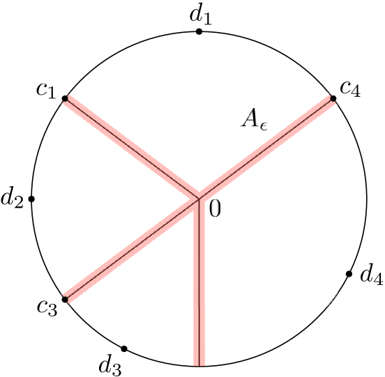
Figure 4. The open tubular neighbourhood $A_{\epsilon}$ of $A$.

In order to prove Lemma 4.3, we need, in particular, to show that the contribution of an $\epsilon$-neighbourhood of $A$ to the value of the integral of the function $\left|\frac{1}{n}\log\big{|}\frac{g^{(n)}(x)}{n!}\big{|}\right|$ can be made arbitrarily small by the choice of $\epsilon$. The rest of the integral will be computed/estimated using Lemma 3.2.

Lemma 4.4.

Under the assumptions of Lemma 4.3, there exists a constant $C$ depending only on $g$ such that for any small enough $\epsilon>0$ and $\delta>0$, and all large enough $n$, one has the inequality

$$\frac{1}{n}\int\limits_{\overline{A_{\epsilon}\cap D(\delta)}}\left|\log\big{|}\frac{g^{(n)}(x)}{n!}\big{|}\right|d\lambda<C\epsilon,$$

where $d\lambda$ is the standard Lebesgue measure on $\mathbb{C}$ and $\overline{A_{\epsilon}\cap D(\delta)}$ is the closure of the intersection of $A_{\epsilon}$ with the disk of radius $\delta$ centered at the origin

The key ingredient of the proof is the classical Cartan-Boutroux lemma (i.e., the Minimum Modulus Principle) which provides an estimate of the growth of $\log|g(x)|$ near its singularities in a form suitable for integration. For the sake of completeness, let us quote the following result from [13] (see also [27]). (In Lemma 4.5, $e$ stands for the standard Euler number, i.e. the base of the natural logarithm.)

Lemma 4.5.

([13, Lecture 11, Theorem 4]) Consider a holomorphic function $g$ on the closed disk $\overline{D(0,2er)}$ with $|g(0)|=1$ and $r>0$. Let $\eta$ be an arbitrary number satisfying $0<\eta<3e/2$ and denote by $M$ the maximal value of $\big{|}g(x)\big{|}$ on the circle $|x|=2er$.

Then there exists a family of (excluded) disks in $\overline{D(0,2er)}$ the sum of radii of which does not exceed $4\eta r$ and such that in the complement to the union of these disks one has the inequality

$$\log|g(x)|>-H(\eta)\log M,$$ (4.2)

where $H(\eta)=2+\log\frac{3e}{2\eta}$.

Remark 4.6.

We want to apply this result for small $\eta$. Note that our condition on $\eta$ implies that:

1. $H(\eta)\geq 2>0$;

2. $H(\eta)\sim-\log\eta$ as $\eta\to 0$;

3. the total area of the excluded discs in Lemma 4.5 is less than $\pi(4\eta R)^{2}$ (since the maximal area occurs in the case of one excluded disk).

Remark 4.7.

If $g(0)\neq 0$, we apply Lemma 4.5 to $g(z)/g(0)$ and modify (4.2) obtaining

$$\log|g(x)|-\log|g(0)| >-H(\eta)(\log M-\log|g(0)|)$$

$$\iff\log|g(x)| >-H(\eta)\log M+(1+H(\eta))\log|g(0)|.$$ (4.3)

We will also make use of a specific covering of $A_{\epsilon}$ by a family of disks.

Lemma 4.8.

For every sufficiently small $\epsilon>0$, there exist $r>0$, $h>0$, and $s_{\epsilon}$ points $x_{1},\dots,x_{s_{\epsilon}}\in A_{\epsilon}\setminus A$ such that the following $3$ conditions are satisfied.

1. $A_{\epsilon}$ is covered by the union of the disks $\bigcup\limits_{i=1}^{s_{\epsilon}}D(x_{i},r)$ of radius $r$ centered at $x_{i}$.

2. The area of the union $\bigcup\limits_{i=1}^{s_{\epsilon}}D(x_{i},r)$ is smaller than $\epsilon C_{A}$ where $C_{A}$ is a constant depending only on $A$.

3. The union $\bigcup\limits_{i=1}^{s_{\epsilon}}D(x_{i},2er+h)$ lies at the distance at least $d/2$ from the points $\{d_{1},\ldots,d_{k}\}$ where $d$ is the distance between $A$ and $\{d_{1},\ldots,d_{k}\}$.

Proof.

Observe that for (3) to be true it suffices that $r$ and $\epsilon$ satisfy the inequality $2er+h<d/2-\epsilon$. Given $\epsilon<d/2$, this is clearly a feasible constraint on $r$ and $h$. The rest of the argument is intuitively clear and can be made precise by using Euclidean geometry. Namely, the domain $A_{\epsilon}$ decomposes into a central $k$-gon (contained in a disk of radius $\epsilon$) and $k$ strips (each contained in a rectangle of length $\rho$ and width $2\epsilon$), see Figure 4. Each of these polygonal pieces can be covered by a family of equilateral triangles of size $\epsilon$ where the number of these equilateral triangles grows at most as $\frac{\rho}{\epsilon}$. We construct a family of disks, each circumscribing an equilateral triangle of the family. Then, the linear in $\epsilon$ bound on the area of the covering family of disks is easily realised. An arbitrarily small deformation of the covering ensures that the centers of the disks do not belong to $A$. Finally, we notice that since $r=r(\epsilon)\to 0$ as $\epsilon$, we have $\lim\limits_{\epsilon\to 0}d/2-\epsilon-2er=d/2$, and we can choose the constant $h$ such that it works for all sufficiently small $\epsilon$. ∎

Let us now settle Lemma 4.4.

Proof of Lemma 4.4.

The argument consists of four steps.

4.2.1. First step

Choose $0<\epsilon<\delta<\rho$ so small that $g$ is holomorphic in $A_{\epsilon}\cap D(\delta)$. Let $r>0$ be such that $\overline{A_{\epsilon}\cap D(\delta)}$ is covered by the disks $D(x_{i},r)$, $i=1,\ldots,s_{\epsilon}$ as in Lemma 4.8. Decreasing if necessary $\delta$ and $\epsilon$, we require that each $D(x_{i},2er+h)$ is contained in $D(\rho)$, where $h$ is a constant independent of $\epsilon$, see the end of the proof of Lemma 4.8. Then, since $x_{i}$ lies outside of $A$, Lemma 3.2 implies that

$$\lim_{n\to+\infty}\frac{1}{n}\log\bigg{|}\frac{g^{(n)}(x_{i})}{n!}\bigg{|}=-\log|x_{i}-d_{i}|=M(x_{i}),$$ (4.4)

where $d_{i}$ is the point nearest to $x_{i}$ among $\{d_{1},\ldots,d_{k}\}$. In particular, $\frac{g^{(n)}(x_{i})}{n!}\neq 0$ for all sufficiently large $n$. Let $n_{0}\in\mathbb{N}$ be such that for all $i=1,\dots,s_{\epsilon}$,

$$\bigg{|}M(x_{i})-\frac{1}{n}\log\big{|}\frac{g^{(n)}(x_{i})}{n!}\big{|}\bigg{|}\leq|M(x_{i})|\text{ if }n>n_{0}.$$ (4.5)

Therefore,

$$\bigg{|}\log\big{|}\frac{g^{(n)}(x_{i})}{n!}\big{|}\bigg{|}\leq C\cdot n,\text{ if }n>n_{0},$$ (4.6)

where $C$ is the maximum of $2|M(x)|$ in a region containing $\overline{A_{\epsilon}\cap D(\delta)}$.

4.2.2. Second step

Condition (3) in Lemma 4.8 and the choice of a small $\delta>0$ ensure that $g$ is holomorphic on the union of the disks $\bigcup\limits_{i=1}^{s_{\epsilon}}D(x_{i},2er+h)$. Let $B$ be the maximal value of $|g(x)|$ on this union. Since circles of radius $h$ around a point $x$ on the circle $|x-x_{i}|=2er$ are contained in $D(x_{i},2er+h)$, we can apply Cauchy’s bound for the (absolute) values of the derivatives of $g$ at a point $x$ with $|x-x_{i}|\leq 2er$ and obtain an estimate

$$\bigg{|}\frac{g^{(n)}(x)}{n!}\bigg{|}\leq h^{-n}B.$$ (4.7)

This inequality is hence true for any $x\in\bigcup\limits_{i=1}^{s_{\epsilon}}D(x_{i},2er)$.

4.2.3. Third step

We now apply Lemma 4.5 to $\frac{g^{(n)}(x)}{n!}$ in each disk $D_{i}=D(x_{i},r)$. Let $M_{n}\leq h^{-n}B$ be the maximum of $\big{|}\frac{g^{(n)}(x)}{n!}\big{|}$ on the circle $|x-x_{i}|=2er$. (This inequality follows from (4.7).)

For small $\eta>0$, let us introduce the subset $O_{\eta,i}\subset D_{i}$ such that for $x\in O_{\eta,i}$, we have

$$\log\left|\frac{g^{(n)}(x)}{n!}\right|>-H(\eta)\left(\log M_{n}-\log\left|\frac{g^{(n)}(x_{i})}{n!}\right|\right)+\log\left|\frac{g^{(n)}(x_{i})}{n!}\right|.$$ (4.8)

Following Lemma 4.5 and Remark 4.7, the subset $O_{\eta,i}$ satisfies the relation

$$\lambda(D_{i}\setminus O_{\eta,i})\leq\pi(4\eta r)^{2}.$$ (4.9)

Inequality 4.9 gives a rough estimate of $\big{|}\log|\frac{g^{(n)}(x)}{n!}|\big{|}$ as follows. First, by (4.7),

$$\log(h^{-n}B)\geq\log\big{|}\frac{g^{(n)}(x)}{n!}\big{|}.$$ (4.10)

Then, by the Maximum Modulus principle,

$$\log(h^{-n}B)-\log\left|\frac{g^{(n)}(x_{i})}{n!}\right|\geq\log M_{n}-\log\left|\frac{g^{(n)}(x_{i})}{n!}\right|\geq 0.$$

Using the latter inequality and the fact that $-H(\eta)<0$, we have that (4.8) implies

$$\log\left|\frac{g^{(n)}(x)}{n!}\right|\geq-H(\eta)\left(\log(h^{-n}B)-\log\left|\frac{g^{(n)}(x_{i})}{n!}\right|\right)+\log\left|\frac{g^{(n)}(x_{i})}{n!}\right|.$$ (4.11)

The standard triangle inequality then implies that for any triple of real numbers $c\geq b\geq a$, we have $|a|+|c|\geq|b|.$ So, (4.10) and (4.11), together with (4.6), imply

$$(|H(\eta)|+1)(|\log(h^{-n}B)|+Cn)\geq\bigg{|}\log\big{|}\frac{g^{(n)}(x)}{n!}\big{|}\bigg{|}.$$ (4.12)

Since $\bigcup\limits_{i=1}^{s_{\epsilon}}D(x_{i},r)=\bigcup\limits_{i=1}^{s_{\epsilon}}D_{i}$ covers $A_{\epsilon}\cap D(\delta)$, we can finally deduce from (4.9) that the subset $O_{\eta}=\bigcup\limits_{i=1}^{s_{\epsilon}}O_{\eta,i}\subset\bigcup\limits_{i=1}^{s_{\epsilon}}D_{i}$, for which the inequality (4.12) holds, satisfies the relation

$$\lambda(\overline{A_{\epsilon}\cap D(\delta)}\setminus O_{\eta})\leq s_{\epsilon}\pi(4\eta r)^{2}=L\eta^{2}\epsilon,$$ (4.13)

for some constant $L$.

4.2.4. Fourth step

Fix some $\epsilon>0$. The inequality (4.13) implies that as $\eta\longrightarrow 0$ the sets $O_{\eta}$ form an exhausting sequence of open subsets for $\overline{A_{\epsilon}\cap D(\delta)}$.

Now, we can estimate the integral

$$\frac{1}{n}\int\limits_{\overline{A_{\epsilon}\cap D(\delta)}}\left|\log\big{|}\frac{g^{(n)}(x)}{n!}\big{|}\right|d\lambda.$$

Set $\eta_{j}=1/j$ and $O_{0}:=\emptyset$ and subdivide the integral as follows:

$$\frac{1}{n}\int\limits_{\overline{A_{\epsilon}\cap D(\delta)}}\left|\log\big{|}\frac{g^{(n)}(x)}{n!}\big{|}\right|d\lambda=\frac{1}{n}\sum\limits_{j=0}^{+\infty}\int_{O_{\eta_{j+1}}\setminus O_{\eta_{j}}}\left|\log\big{|}\frac{g^{(n)}(x)}{n!}\big{|}\right|d\lambda.$$ (4.14)

By (4.12) and (4.13), the last sum is dominated by

$$\frac{1}{n}\sum\limits_{j=1}^{+\infty}\frac{L\epsilon}{j^{2}}|(|H(1/j)|+1)(|\log(h^{-n}B)|+Cn).$$ (4.15)

Now, observe that $|H(1/j)|+1\sim\log j$ by Remark 4.6. Secondly, $\frac{|\log(h^{-n}B)|+Cn}{n}$ is globally bounded (recall that $h$ is a constant, independent of $\epsilon$). Hence, (4.15) converges to $\epsilon S_{n}$, for some uniformly bounded $S_{n}$. This is the desired bound, and Lemma 4.4 is proved.

4.2.5. Proof of Lemma 4.3

By choosing sufficiently small $\epsilon$ and $\delta$, Lemma 3.2 guarantees that the integral of $\left|\frac{1}{n}\log\left|\frac{g^{(n)}(x)}{n!}\right|-M(x)\right|d\lambda$ on $\overline{D}(\delta)\setminus A_{\epsilon}$ converges uniformly to zero. It remains to show that the integral of the same measure over $\overline{A_{\epsilon}\cap D(\delta)}$ can be made arbitrarily small as $\epsilon\rightarrow 0$.

By choosing a small enough $\delta$, we achieve that $|M(x)|$ can be globally bounded on $\overline{D}(\delta)$ while the area of $A_{\epsilon}\cap D(\delta)$ can be bounded by a linear expression in $\epsilon$. Together we obtain that

$$\int\limits_{\overline{A_{\epsilon}\cap D(\delta)}}\left|M(x)\right|d\lambda<B\cdot\epsilon$$

for some constant $B>0$.

Using the estimate of Lemma 4.4 (proved in Sections 4.2.1 - 4.2.4), we conclude that

$$\int\limits_{\overline{A_{\epsilon}\cap D(\delta)}}\left|\frac{1}{n}\log\left|\frac{g^{(n)}(x)}{n!}\right|\right|d\lambda<C\cdot\epsilon$$

for some constant $C$ independent of $n$.

By the triangle inequality, we deduce that $\int\limits_{\overline{A_{\epsilon}\cap D(\delta)}}\left|\frac{1}{n}\log\left|\frac{g^{(n)}(x)}{n!}\right|-M(x)\right|d\lambda$ can be made arbitrarily small as $\epsilon\rightarrow 0$. This proves the convergence of the integral over $\overline{D}(\delta)$ to zero. ∎

4.3. Laplace operator acting on $L^{1}_{loc}(X^{\ast})$

As we discussed above, on the surface $X^{\ast}$ obtained from $X$ by puncturing it at the poles of $\omega$, there is a natural singular flat metric $|\omega|$ with conical singularities at the zeros of $\omega$. Let us denote by $\Delta_{\omega}$ the corresponding Laplace operator defined on $L^{1}_{loc}(X^{\ast})$; see [10, 12] for details on Laplace operators for singular flat metrics.

It acts on $L^{1}_{loc}(X^{\ast})$, and in particular, with respect to the parametrising variable it coincides with the standard Laplace operator $\Delta=\frac{\partial^{2}}{\partial x^{2}}+\frac{\partial^{2}}{\partial y^{2}}$ acting on test functions in a local parametrisation, even at the singular points of the flat metric, see [10, Proposition 3.3 and (4.3)]. This allows us to compute the Laplacian of $T_{\omega}^{n}f$, considered first as a distribution.

Lemma 4.9.

For some $N\in\mathbb{N}$ and any $n\geq N$, one has

$$\frac{1}{2\pi}\Delta_{\omega}\log\left|T_{\omega}^{n}f(z)\right|=\sum_{z\in Z(T_{\omega}^{n}f)}\ \delta_{z}-n\left(\sum_{p\in\mathcal{PPL}(\omega,f)}\delta_{p}\right)-\nu,$$

where $Z(T_{\omega}^{n}f)$ is the set of the zeros of $T_{\omega}^{n}f$ in $X^{\ast}$ (counted with multiplicities) and $\nu$ is a fixed measure of finite mass and support.

Proof.

Take $z_{0}\in X^{\ast\ast}$ obtained from $X$ by puncturing it at the zeros and the poles of $\omega$. For any small enough neighbourhood $U$ of $z_{0}$, a local primitive $\phi$ of $\omega$ such that $\phi(z_{0})=0$ defines a local flat chart in which the operator $\Delta_{\omega}$ is conjugated to the standard Laplace operator $\Delta$. Since $T_{\omega}^{k}(f)=g^{(k)}\circ\phi$ in $U$, we have

$$\Delta_{\omega}\log\left|T_{\omega}^{n}f(z)\right|=(\Delta\log\left|g^{(n)}\right|)\circ\phi(z).$$ (4.16)

It is well-known that the standard Laplacian of the logarithm of the absolute value of a meromorphic function $f$, considered as a $L^{1}_{loc}$-function (and hence as a distribution), is the divisor of $f$ expressed in terms of Dirac measures. We deduce that on any open subset of $X^{\ast\ast}$, $\frac{1}{2\pi}\Delta_{\omega}\log\left|T_{\omega}^{n}f(z)\right|$ coincides with the divisor of the zeros and poles of $f^{(n)}$ (taken as a distribution). Following the results of Section 2.1, the poles of $T_{\omega}^{n}f$ lying in $X^{\ast\ast}$ are located at the poles of $f$. They belong to $\mathcal{PPL}(\omega,f)$ and the order of each of them increases by one after each application of $T_{\omega}$. This proves the required claim for any open subset of $X^{\ast}$ not containing a zero of $\omega$.

Now consider an arbitrarily small open neighbourhood $U$ of a zero $z_{0}$ of $\omega$. There locally exists a primitive $\zeta=\phi$ of $\omega$ that maps the open set $U$ to an open set $V$ in the $\zeta$-plane as a branched cover.

In the first case, $z_{0}\notin\mathcal{PPL}(\omega,f)$ and $f=g\circ\phi$ is locally factorised by a primitive $\zeta=\phi$ of $\omega$ (see Definition 1.2). By the remark on the Laplacian before the proof, the equality (4.16) still holds, and the same argument as above gives that

$$\Delta_{\omega}\log\left|T_{\omega}^{n}f(z)\right|=\sum_{z\in Z(T_{\omega}^{n}f)\cap U}\ \delta_{z}$$

as a distribution on $X^{\ast}$ (where we use the local coordinates of the complex structure on the Riemann surface).

In the second case, $z_{0}\in\mathcal{PPL}(\omega,f)$ and $T_{\omega}^{n}f$ has a pole in $z_{0}$ provided $n$ is large enough, see Proposition 2.2. Moreover, if $U$ is small enough, Proposition 3.1 shows that $T_{\omega}^{n}f$ has no zeros in $U$. In terms of the local variable $\zeta=\phi(z)$, we have that the function $f(z)=g(\zeta^{1/k})$ can be expanded in a Puiseux series, and then, by Lemma A.4, locally in $U$ we have the equality

$$\frac{1}{2\pi}\Delta_{\omega}\log\left|T_{\omega}^{n}f(z)\right|=-(n+\alpha(n))\delta_{p},$$

where $\alpha(n)$ is bounded. Finally, let $\nu$ be the measure given as the sum of all constant parts $\alpha(n)\delta_{p}$ together with a similar sum coming from the poles of $f$ at the regular points. ∎

In Proposition 4.1 we have shown that $\dfrac{1}{n}\log\left|\frac{T_{\omega}^{n}f(z)}{n!}\right|$ converges to $\log\frac{1}{\rho(z)}$ in $L^{1}_{loc}(X^{\ast}\setminus\mathcal{PPL}(\omega,f))$. We deduce that $\Delta_{\omega}\dfrac{1}{n}\log\left|\frac{T_{\omega}^{n}f(z)}{n!}\right|$ converges to $\Delta_{\omega}\log\frac{1}{\rho(z)}$ as a distribution. Let us prove that the Laplacian of $\log\frac{1}{\rho(z)}$ can be computed in terms of the Cauchy measure of the Voronoi diagram defined by $f$ and $\omega$.

Lemma 4.10.

We have the equality of distributions on $X^{\ast}$ given by

$$\frac{1}{2\pi}\Delta_{\omega}\log\frac{1}{\rho(z)}=\mu_{\omega,f}-\sum_{p\in\mathcal{PPL}(\omega,f)}\ \delta_{p}.$$

where $\rho(z)$ is the critical radius of the Voronoi function $g_{z}$ (see Definition 2.5) and $\mu_{\omega,f}$ is the Cauchy measure of $\mathcal{V}_{\omega,f}$ (see Section 2.5).

Proof.

Note first that in a chart $\zeta=\phi(z)$ the Laplace operator acting on test or real analytic functions such as as $\log(\frac{1}{\rho(z)})$ can be expressed as

$$\frac{1}{2\pi}\Delta_{\omega}=\frac{2}{\pi}\frac{\partial^{2}}{\partial\bar{\zeta}\partial\zeta}.$$

Thus it suffices to prove Lemma 4.10 in a distinguished parameter $\zeta$ and for a corresponding open set $V$. In a small enough neighbourhood of $p\in\mathcal{PPL}(\omega,f)$, we have that $\rho(\zeta)=|\zeta-p|$, and $\frac{1}{2\pi}\Delta_{\omega}\log(\frac{1}{\rho(\zeta)})=-\delta_{p}$. This gives the Dirac delta function part in the formulation of the lemma. Besides these terms, the support of the Laplacian will be contained in the Voronoi skeleton, since $\rho$ is harmonic in each (open) Voronoi cell. Next, take a small neighbourhood $N$ intersecting the Voronoi skeleton and containing no points of $\mathcal{PPL}(\omega,f)$. Let $p_{i}\ i=1,\dots$ be the points in $\mathcal{PPL}(\omega,f)$ such that the relation $\rho(\zeta)=|\zeta-p_{i}|$ is valid in a non-zero open subset $O_{i}$ of $N$. Define $H_{i}(\zeta):=-\log|\zeta-p_{i}|$ which is a harmonic function in the complex plane except for $\zeta=p_{i}$. Let $\chi_{i}$ be the characteristic function of $O_{i}$. One has the equality of $L^{1}_{loc}$-functions given by $M(z):=\log(\frac{1}{\rho(\zeta)})=\sum H_{i}(\zeta)\chi_{i}$.

Next, we need to recall how to calculate the derivatives of a characteristic function using the Sokhotski-Plemelj formula. Let $g$ be a test function (with compact support) which by assumption, vanishes on the part of each $\partial O_{i}$ not contained in the Voronoi skeleton. Finally, let $\partial_{v}$ denote the directional derivative associated to a vector $v=(\alpha,\beta)$ in $\mathbb{C}\simeq\mathbb{R}^{2}$.

Green’s theorem (in its normal form) implies that

$$-\langle\partial_{v}\chi_{i},g\rangle=\int\int_{O_{i}}\partial_{v}gdxdy=\int_{\partial O_{i}}(\alpha,\beta)\cdot Ngds,$$ (4.17)

where the boundary $\partial O_{i}$ is oriented so that $O_{i}$ is located to the left, and $N_{i}$ is the unit normal pointing away from $O_{i}$. Note that, in the chosen orientation we get $Nds=(dy,-dx)$. In terms of distributions (and with a slight abuse of notation), this can be formulated as

$$\partial_{v}\chi_{i}=-(\alpha,\beta)\cdot Nds=-\alpha dy+\beta dx,$$ (4.18)

which remains true even if $v$ is a complex vector. As a first corollary, Leibniz’ rule implies the following equality of distributional derivatives

$$\frac{\partial M(\zeta)}{\partial\zeta}=\sum\frac{\partial H_{i}(\zeta)}{\partial\zeta}\chi_{i},$$ (4.19)

since each part of the boundary $V_{ij}$ between the cells $O_{i}$ and $O_{j}$ occurs twice with opposite normals in the second part of the sum

$$\frac{\partial M(\zeta)}{\partial\zeta}=\sum_{i}\frac{\partial H_{i}(\zeta)}{\partial\zeta}\chi_{i}-\sum_{i}H_{i}(\zeta)(\frac{1}{2})(1,-i)\cdot N_{i}ds,$$

and $M(\zeta)$ is continuous on $V_{ij}$. (Clearly the endpoints of $V_{ij}$ (at which the normal is undefined) do not contribute to the integral (4.17)). Thus the distributional derivative coincides almost everywhere with the pointwise derivative (and is also a bona fide $L^{1}_{loc}$-function). Applying (4.18) and one more Leibniz rule to (4.19) we get

$$\frac{\partial^{2}M(\zeta)}{\partial\bar{\zeta}\partial\zeta}=\sum\frac{\partial^{2}H_{i}(\zeta)}{\partial\bar{\zeta}\partial\zeta}\chi_{i}-\sum\frac{1}{2}\frac{\partial H_{i}(\zeta)}{\partial\zeta}(1,i)\cdot Nds,$$ (4.20)

since $\frac{\partial}{\partial\zeta}=\frac{1}{2}(\frac{\partial}{\partial x}+i\frac{\partial}{\partial y})$. The first sum vanishes by our assumptions on $N$. Concerning the second sum, note that a) $\frac{\partial H_{i}(\zeta)}{\partial\zeta}=1/(2(\zeta-a_{i}))$, and b) since $Nds=(dy,-dx)$ we get $(1,i)\cdot N\mathop{}\!\mathrm{d}s=\mathop{}\!\mathrm{d}y-i\mathop{}\!\mathrm{d}x=-i\mathop{}\!\mathrm{d}\zeta$.

Each piece of $V_{ij}$ separating the Voronoi cell $O_{i}$ (located to the left) from $O_{j}$, will occur twice in the sum, and thus

$$(-i/4)(\frac{1}{z-a_{i}}-\frac{1}{z-a_{j}})\mathop{}\!\mathrm{d}z=(i/4)\frac{a_{j}-a_{i}}{(z-a_{i})(z-a_{j})}\mathop{}\!\mathrm{d}z.$$ (4.21)

Observe that $V_{ij}$ is an interval of the orthogonal midline to the straight segment between $a_{i}$ and $a_{j}$, which is given by the equation

$$\zeta=(1/2)(a_{i}+a_{j})+ti(a_{j}-a_{i})=(1/2-ti)a_{i}+(1/2+ti)a_{j},\ t\in\mathbb{R}.$$

Then, if $\zeta\in V_{ij}$, we get $\zeta-a_{i}=(a_{j}-a_{i})(1/2+ti)$ and $\zeta-a_{j}=-(a_{j}-a_{i})(1/2-ti)$. Using the orientation which places $O_{i}$ to the left of $V_{ij}$, and $\mathop{}\!\mathrm{d}\zeta=i(a_{j}-a_{i})\mathop{}\!\mathrm{d}t$, the measure in (4.21) is given by

$$\frac{\mathop{}\!\mathrm{d}t}{4(1/4+t^{2})}=\frac{|a_{i}-a_{j}|^{2}dt}{4|\zeta-a_{i}||\zeta-a_{j}|}.$$

Here we use the relation $|\zeta-a_{i}||\zeta-a_{j}|=|\zeta-a_{i}|^{2}=|a_{j}-a_{i}|^{2}((1/4)+t^{2})$. The standard length measure on $V_{ij}$ is given by $\mathop{}\!\mathrm{d}s=|a_{j}-a_{i}|\mathop{}\!\mathrm{d}t.$ To finish the proof, it just remains to observe that the latter relation multiplied by $\frac{2}{\pi}$ is exactly the Cauchy measure, see Definitions 2.13 and 2.14. ∎

4.4. Tying up the loose ends

We are now ready to prove our main result.

Proof of Theorem 1.5.

In Proposition 4.1, we have shown that $\dfrac{1}{n}\log\left|\frac{T_{\omega}^{n}f(z)}{n!}\right|$ converges to $\log\frac{1}{\rho(z)}$ in the space of locally integrable functions on $X^{\ast}\setminus\mathcal{PPL}(\omega,f)$. Introducing the Laplace operator $\Delta_{\omega}$ corresponding to the flat metric $|\omega|$ on $X^{\ast}$ (see Section 4.3), we obtained that $\Delta_{\omega}\log\left|T_{\omega}^{n}f(z)\right|^{1/n}$ converges to $\Delta_{\omega}\log\frac{1}{\rho(z)}$ as distributions on $X^{\ast}$.

These distributions have been computed in Lemma 4.9 and Lemma 4.10. We concluded that $\frac{1}{n}\sum_{z\in Z(T_{\omega}^{n}f)}\ \delta_{z}$ converges to $\mu_{\omega,f}$ as positive distributions of finite weight on $X^{\ast}$. In other words, the zeros of $T_{\omega}^{n}f$ in the punctured surface $X^{\ast}$ asymptotically distribute according to the Cauchy measure of the Voronoi diagram $\mathcal{V}_{\omega,f}$ (see Section 2.5). In particular, the Voronoi diagram is contained in the limit set $\mathcal{L}(T_{\omega},f)$.

An immediate computation proves that at a pole $p$ of $\omega$ of order $d$, for any large enough $n$, $T_{\omega}^{n}(f)$ has a zero at $p$ of order $(d-1)n+b$ where $b$ is some constant determined by the order of $f$ at $p$. From this fact we conclude the following:

• if $d\geq 2$, then $p\in\mathcal{L}(T_{\omega},f)$;

• if $d=1$, then $p\in\mathcal{L}(T_{\omega},f)$ if and only if $p$ is not a pole of $f$.

Combining this information with Proposition 3.1 claiming that any relatively compact open subset in a Voronoi cell is zero-free provided $n$ is large enough, we obtain the complete description of $\mathcal{L}(T_{\omega},f)$ as a subset of $X$, proving claim (i) of Theorem 1.5.

It remains to compute the asymptotic root-counting measure of the sequence $(T_{\omega}^{n}(f))_{n\in\mathbb{N}}$. It has been shown in Corollary 2.3 that the sum $\mathcal{Z}_{n}$ of orders of the poles of meromorphic function $T_{\omega}^{n}(f)$ (and therefore the sum of orders of its zeros) has the asymptotics $\mathcal{Z}_{n}\sim An$ as $n\rightarrow\infty$ where

$$A=\sum\limits_{z\in\mathcal{PPL}(\omega,f)}(a_{z}+1).$$

Therefore the asymptotic root-counting measure of the sequence $(T_{\omega}^{n}(f))_{n\in\mathbb{N}}$ is the sum of $\frac{1}{A}\mu_{\omega,f}$ (corresponding to the contribution of the punctured surface $X^{\ast}$) and the term $\frac{1}{A}(d_{p}-1)\delta_{p}$ for each pole of $\omega$. ∎

Remark 4.11.

The computation of the asymptotic root-counting measure proves in particular that the Cauchy measure $\mu_{\omega,f}$ of the Voronoi diagram $\mathcal{V}_{\omega,f}$ is an integer multiple of $\pi$ which is a topological invariant of the pair $(\omega,f)$ in the spirit of the Gauss-Bonnet formula.

5. Application to derivatives of algebraic functions

Our approach strengthens and generalises the earlier results of Prather-Shaw in [18, 19] on the derivatives of (a restricted class of) algebraic functions.

Notation 5.1.

Consider a plane algebraic curve $\Gamma\subset\mathbb{C}_{z}\times\mathbb{C}_{w}$ with coordinates $(z,w)$ given as the zero locus of a bivariate polynomial $\Phi(z,w)=0$. Take the projectivization $\widetilde{\Gamma}\subset\mathbb{C}P^{1}_{z}\times\mathbb{C}P^{1}_{w}$ of $\Gamma$ in $\mathbb{C}P^{1}_{z}\times\mathbb{C}P^{1}_{w}$ with homogeneous coordinates $(Z_{0}:Z_{1}),(W_{0}:W_{1})$. Denote the bidegree of $\widetilde{\Gamma}$ by $(k,\ell)$. To avoid trivialities we assume that both $k$ and $\ell$ are positive. The case of rational functions considered by Pólya corresponds to the situation $\ell=1,\;k\geq 2$.

Notation 5.2.

In the above notation, consider the projection $\pi_{z}:\widetilde{\Gamma}\to\mathbb{C}P^{1}_{z}$. Under the assumption that $\Gamma$ is reduced the preimage $\pi_{z}^{-1}(\hat{z})\subset\widetilde{\Gamma}$ of a generic point $\hat{z}\in\mathbb{C}P^{1}$ consists of $\ell$ distinct points. By the branching locus $\mathcal{B}(\Gamma)\subset\mathbb{C}P^{1}_{z}$ we mean the set of points $\hat{z}\in\mathbb{C}P^{1}_{z}$ for which $\pi_{z}^{-1}(\hat{z})\subset\mathbb{C}P^{1}_{w}$ is a positive divisor of degree $\ell$ with less than $\ell$ distinct points, i.e. some point has multiplicity exceeding $1$. Points of multiplicity more than $1$ in the preimage $\pi_{z}^{-1}(\hat{z})$ of a branching point $\hat{z}$ will be called the critical points of (the meromorphic function) $\pi_{z}:\widetilde{\Gamma}\to\mathbb{C}P^{1}_{z}$.

The affine branching locus $\mathcal{B}_{a}(\Gamma)$ is not just the restriction of $\mathcal{B}(\Gamma)$ to $\mathbb{C}_{z}$, but is its subset for which we additionally require that for $\hat{z}\in\mathcal{B}_{a}(\Gamma)$ at least one critical point of the divisor $\pi^{-1}_{z}(\hat{z})$ is affine, i.e. lies in $\mathbb{C}_{w}$ and not at $\infty_{w}\in\mathbb{C}P^{1}_{w}$.

We call a critical point $\hat{w}\in\pi_{z}^{-1}(\hat{z})|_{\mathbb{C}_{w}}$ essential if at least one of the local branches of $\Gamma$ near $\hat{w}$ has a critical point at $\hat{w}$ as well, i.e. its projection on a small neighbourhood of $\hat{z}$ is not a local biholomorphism. (In other words, this branch needs fractional powers for its presentation as a Puiseux series at $\hat{z}$ or, alternatively, $\hat{z}$ is a branch point of the lift $n\pi_{z}:N\widetilde{\Gamma}\to\mathbb{C}P^{1}_{z}$ where $N\widetilde{\Gamma}$ is the normalisation of $\widetilde{\Gamma}$.) The branching point $\hat{z}\in\mathcal{B}_{a}(\Gamma)$ obtained as projection of an essential critical point $\hat{w}$ to $\mathbb{C}P^{1}_{z}$ is called essential as well. Let $\mathcal{B}_{a}^{ess}(\Gamma)\subset\mathcal{B}_{a}(\Gamma)$ denote the set of all essential affine branching points.

Finally, by the locus of poles $\mathcal{P}(\Gamma)\subset\mathbb{C}P^{1}_{z}$ we mean the set of points $\hat{z}\in\mathbb{C}P^{1}_{z}$ for which $\pi_{z}^{-1}(\hat{z})\subset\mathbb{C}P^{1}_{w}$ contains $\infty_{w}\in\mathbb{C}P^{1}_{w}$ where $\mathbb{C}P^{1}_{w}=\mathbb{C}_{w}\cup\infty$. The affine locus of poles $\mathcal{P}_{a}(\Gamma)\subset\mathcal{P}(\Gamma)$ is the restriction of $\mathcal{P}(\Gamma)$ to $\mathbb{C}_{z}$.

Definition 5.3.

Given $\Gamma$ as above and a positive integer $n$, define the algebraic curve $\Gamma^{(n)}\subset\mathbb{C}_{z}\times\mathbb{C}_{w}$, called the affine $n$-th derivative curve, obtained by taking the $n$-th derivatives of all branches of $\Gamma$ considered as (local) algebraic function $w(z)$ with respect to the variable $z$. The $n$-th derivative curve of $\Gamma$ is the projectivization $\widetilde{\Gamma}^{(n)}\subset\mathbb{C}P^{1}_{z}\times\mathbb{C}P^{1}_{w}$ of $\Gamma^{(n)}$.

Definition 5.4.

We define the (projective) zero locus $\widetilde{\mathcal{Z}}^{(n)}(\Gamma)$ of the $n$-th derivative of the algebraic function given by the algebraic curve $\Gamma$ as the intersection locus of $\widetilde{\Gamma}^{(n)}$ with $(\mathbb{C}P^{1}_{z},0)\subset\mathbb{C}P^{1}_{z}\times\mathbb{C}P^{1}_{w}$. The affine zero locus $\mathcal{Z}_{a}^{(n)}(\Gamma)$ is the restriction of $\widetilde{\mathcal{Z}}^{(n)}(\Gamma)$ to $\mathbb{C}_{z}\subset\mathbb{C}P^{1}_{z}$. The (projective) limit set $\mathcal{F}(\Gamma)\subset\mathbb{C}P^{1}_{z}$ is the limiting set of the supports of the sequence $\{\widetilde{\mathcal{Z}}^{(n)}(\Gamma)\}$ and the affine limit set $\mathcal{F}_{a}(\Gamma)\subset\mathbb{C}_{z}$ is the limit set of the supports of the sequence $\{\widetilde{\mathcal{Z}}^{(n)}_{a}(\Gamma)\}\subset\mathbb{C}_{z}$.

Remark 5.5.

In Pólya’s original definition, see [16], the limit set for the usual derivative of a rational function consists of all points every neighbourhood of which contains points from infinitely many $\widetilde{\mathcal{Z}}_{a}^{(n)}(\Gamma)$.

Problem 5.6.

Given an affine (resp. projective) reduced algebraic curve $\Gamma$ as above, describe its affine (resp. projective) limit set.

Remark 5.7.

Obviously, if the bidegree of $\Gamma$ is $(k,1)$ we recover the classical question of Pólya about the accumulation of zeros of consecutive derivatives of a rational function. Moreover for algebraic functions given by a certain class of algebraic curves, their limit sets have been described in [19]. However, to the best of our knowledge, the description of the limit set for general reduced algebraic curves is new.

To derive results about the limit sets of general algebraic curves, i.e. about the accumulation of the zeros of consecutive derivatives of algebraic functions from the material of the previous sections we proceed as follows. Our main objects are as follows.

Definition 5.8.

Given a reduced affine curve $\Gamma\subset\mathbb{C}_{z}\times\mathbb{C}_{w}$, take the normalisation $N\widetilde{\Gamma}$ of the projectivization $\widetilde{\Gamma}\subset\mathbb{C}P^{1}_{z}\times\mathbb{C}P^{1}_{w}$ and define the meromorphic $1$-form $\tilde{\omega}$ on $\widetilde{\Gamma}$ as the pullback of the standard meromorphic $1$-form $dz$ on $\mathbb{C}P^{1}_{z}$ under the projection $\pi_{z}:\widetilde{\Gamma}\to\mathbb{C}P^{1}_{z}$. Then take the pullback $\omega$ of $\tilde{\omega}$ from $\tilde{\Gamma}$ to $N\widetilde{\Gamma}$. The meromorphic function $f:N\widetilde{\Gamma}\to\mathbb{C}P^{1}_{w}$ is obtained as composition of the normalisation map $n:N\widetilde{\Gamma}\to\widetilde{\Gamma}$ with the projection $\pi_{w}:\widetilde{\Gamma}\to\mathbb{C}P^{1}_{w}$.

Lemma 5.9.

In the above notation, the principal polar locus (see Definition 1.3) $\mathcal{PPL}(\omega,f)$ of the pair $(\omega,f)$ on Riemann surface $N\widetilde{\Gamma}$ is given by:

• preimage under the normalisation map $n:N\widetilde{\Gamma}\to\widetilde{\Gamma}$ of the intersection $\widetilde{\Gamma}\cap(\mathbb{C}P^{1}_{z},\infty_{w})$ except possibly for the point $(\infty_{z},\infty_{w}$), see Remark 5.10;

• preimage under the normalisation map $n:N\widetilde{\Gamma}\to\widetilde{\Gamma}$ of the set of all affine essential critical points of $\widetilde{\Gamma}$.

The principal polar locus is non-empty provided $\ell\geq 2$.

Remark 5.10.

There is a simple criterion when the projectivization in $\mathbb{C}P^{1}_{z}\times\mathbb{C}P^{1}_{w}$ of an algebraic curve $\Gamma\subset\mathbb{C}_{z}\times\mathbb{C}_{w}$ given by a bivariate polynomial $\Phi(z,w)=0$ passes through the point $(\infty_{z},\infty_{w})$. Obviously, this happens if and only if there is a branch of the algebraic function $w(z)$ which tends to $\infty_{w}$ when $z\to\infty_{z}$. The latter condition can be reformulated in terms of the Newton polygon $\mathcal{N}_{\Phi}$ of $\Phi(z,w)$. Namely, this happens if and only if $\mathcal{N}_{\Phi}$ contains an edge with a negative slope and such that $\mathcal{N}_{\Phi}$ lies below the line spanned by this edge. This statement can be easily deduced from the known results of Section 38, Th. 63–66 in [4] and Ch. 4, Sections 3 and 4 in [24].

Proof of Lemma 5.9.

Firstly we describe the poles of $f$ and the zeros and poles of $\omega$. Poles of $f$ coincide with $f^{-1}(\infty_{w})$ where $\mathbb{C}P^{1}_{w}=\mathbb{C}_{w}\cup\infty_{w}$. In other words, it is the set of points on $N\widetilde{\Gamma}$ where $\widetilde{\Gamma}$ intersects the projective line $\mathbb{C}P^{1}_{z}\times\infty_{w}\subset\mathbb{C}P^{1}_{z}\times\mathbb{C}P^{1}_{w}$.

Next, the singular points on $\widetilde{\Gamma}$ which project to the affine part $\mathbb{C}_{z}\subset\mathbb{C}P^{1}_{z}$ give rise to zeros of $\omega$ on $N\widetilde{\Gamma}$. We will show a bit later that the singularities of $\widetilde{\Gamma}$ projecting to $\infty_{z}\in\mathbb{C}P^{1}_{z}$ result in poles of $\omega$.

Indeed each local singular branch of $\widetilde{\Gamma}$ near a point $z_{0}\in\mathbb{C}_{z}$ can be represented by a Puiseux series

$$w(z)=\sum_{j\geq\ell}a_{j}(z-z_{0})^{j/k}$$

where $k\geq 2$. This branch can be parameterised by $z(t)=z_{0}+t^{k}$ and $w(t)=\sum_{j=\ell}^{\infty}a_{j}t^{j}$. Here $t$ can be considered as a local chart on $N\widetilde{\Gamma}$ centered at the point mapped to the singularity of the singular branch of $\widetilde{\Gamma}$ under consideration. Since $z=z_{0}+t^{k}$ one has that $dz=t^{k-1}dt$. Therefore $\omega$ being the pullback of $dz$ acquires a zero of order $k-1>1$ at this point.

Furthermore let $y=\frac{1}{z}$ be the local coordinate near $\infty_{z}\in\mathbb{C}P^{1}_{z}$. With respect to $y$, one has $dz=-\frac{1}{y^{2}}dy.$ For any branch of $\widetilde{\Gamma}$ which is non-singular in a small neighbourhood of $\infty_{z}$, i.e. $y=0$ the pullback of $dz$ to this branch will acquire a pole of order $2$.

Finally, let us assume that $\widetilde{\Gamma}$ has a singular local branch near infinity whose Puiseux series is given by

$$w(y)=\sum_{j\geq\ell}a_{j}y^{j/k}.$$

We can parametrise this branch as $y=t^{k}$ and $w(t)=\sum_{j\geq\ell}a_{j}t^{j}.$ The pullback of $dz=-\frac{1}{y^{2}}dy$ to the local coordinate $t$ on $N\widetilde{\Gamma}$ equals $-\frac{k}{t^{k+1}}dt,$ i.e. it has a pole of order $k+1>2$ at the respective point.

Now by definition, $\mathcal{PPL}(\omega,f)$ consists of (a) poles of $f$ that are not poles of $\omega$ and (b) zeros of $\omega$ at which $f$ is not locally factorised by a primitive of $\omega$. Poles of $f$ which are also poles of $\omega$ are preimages of the point $(\infty_{z},\infty_{w})\in\mathbb{C}P^{1}_{z}\times\mathbb{C}P_{w}^{1}$. If $\Gamma$ has branches which tend to $\infty_{w}$ when $z\to\infty_{z}$ then $\widetilde{\Gamma}$ contains $(\infty_{z},\infty_{w})$ and such points exist. Whether $\Gamma$ has such branches is described in the above Remark.

Finally let us show that at each zero of $\omega$ the function $f$ can not be locally factorised by a primitive of $\omega$. As we have already shown zeros of $\omega$ come from the singularities of $\widetilde{\Gamma}$ which project to $\mathbb{C}_{z}$. Since $\omega$ is the pullback of $dz$ and $f$ is the pullback of the coordinate $w$ the factorisability of $f$ by a primitive of $\omega$ in simple words means that for the original branch of $\Gamma$, the algebraic function $w(z)$ is (locally) holomorphic in $z$ which contradicts the assumption that we consider a singular branch.

In order to prove that the principal polar locus is non-empty, we just observe that for $\ell\geq 2$ the meromorphic function $f:N\widetilde{\Gamma}\to\mathbb{C}P^{1}_{w}$ is a ramified cover branched over at least two points of $\mathbb{C}P^{1}_{w}$. Since at least one of these two points is not $\infty_{w}$ and $\ell\geq 2$, $\omega$ has at least one zero. ∎

Applying Theorem 1.5 we obtain that the zeros of $T^{n}_{\omega}(f)$ accumulate on the Voronoi diagram of the Riemann surface $N\widetilde{\Gamma}$ with the measure described in Section 2.5. The limit set of the algebraic function given by the curve $\Gamma$ and the respective measure of this limit set on $\mathbb{C}P^{1}_{z}$ are obtained as the push-forward of the respective objects from $\mathcal{N}\widetilde{\Gamma}$ to $\mathbb{C}P^{1}_{z}$.

More explicitly, we get the following.

Corollary 5.11.

For any reduced algebraic curve $\Gamma\subset\mathbb{C}_{z}\times\mathbb{C}_{w}$, the affine limit set $\mathcal{F}_{a}(\Gamma)\subset\mathbb{C}_{z}$ coincides with the push-forward of the Voronoi diagram of the pair $(\omega,f)$ on $N\widetilde{\Gamma}$ under the projection $\pi_{z}$ to $\mathbb{C}P^{1}_{z}$.

Let us present some explicit examples of $\Gamma=\Gamma_{0}$, $\Gamma_{n}$ for $n\geq 1$ and illustration of the zeros of consecutive derivatives of the occurring algebraic functions.

Example 1. Let $\Gamma_{0}:=\Gamma$ be the curve defined by $w^{\ell}=\frac{P(z)}{Q(z)}$ for some polynomials $P(z)$ and $Q(z)$.

Lemma 5.12.

The curve $\Gamma_{n}:=\Gamma^{(n)}$ is given by the equation

$$w^{\ell}=\frac{V_{n}^{\ell}(z)}{\ell^{n\ell}P(z)^{n\ell-1}Q(z)^{n\ell+1}}$$ (5.1)

where $V_{n}(z)$ is a polynomial determined by the recurrence relation

• $V_{0}(z)=1$,

• $V_{n+1}(z)=\ell P(z)Q(z)V_{n}^{\prime}(z)-((n\ell-1)P^{\prime}(z)Q(z)+(n\ell+1)P(z)Q^{\prime}(z))V_{n}(z)$.

In particular, if $P$ and $Q$ has degrees $d_{1}$ and $d_{2}$, respectively, then

1. $V_{n}(z)$ has degree $n(d_{1}+d_{2}-1)$ and

2. $\Gamma_{n}$ has bidegree $(\max\{n\ell(d_{1}+d_{2})-n\ell,n\ell(d_{1}+d_{2})+(d_{2}-d_{1})\},\ell)$.

Proof.

The base case $n=0$ is clear. Assuming $\Gamma_{n}$ has the form in (5.1) and writing the denominator in (5.1) as $W_{n}$, we have

$$\ell(w^{(n)})^{\ell-1}w^{(n+1)}=\frac{V_{n}^{\ell-1}(\ell W_{n}V_{n}^{\prime}-V_{n}W_{n}^{\prime})}{W_{n}^{2}}$$

and

$$(w^{(n+1)})^{\ell} =\left(\frac{W_{n}^{(\ell-1)/\ell}}{\ell V_{n}^{\ell-1}}\cdot\frac{V_{n}^{\ell-1}(\ell W_{n}V_{n}^{\prime}-V_{n}W_{n}^{\prime})}{W_{n}^{2}}\right)^{\ell}$$

$$=\frac{(\ell W_{n}V_{n}^{\prime}-V_{n}W_{n}^{\prime})^{\ell}}{\ell^{\ell}W_{n}^{\ell+1}}.$$

Substituting back $W_{n}$ and simplifying yields

$$(w^{(n+1)})^{\ell} =\frac{(\ell^{n\ell}P^{n\ell-2}Q^{n\ell})^{\ell}(\ell PQV_{n}^{\prime}-V_{n}((n\ell+1)PQ^{\prime}+(n\ell-1)P^{\prime}Q)^{\ell}}{\ell^{\ell}(\ell^{n\ell}P^{n\ell-1}Q^{n\ell+1})^{\ell+1}}$$

$$=\frac{(\ell PQV_{n}^{\prime}-V_{n}((n\ell+1)PQ^{\prime}+(n\ell-1)P^{\prime}Q)^{\ell}}{\ell^{\ell(n+1)}P^{\ell(n+1)-1}Q^{\ell(n+1)+1}}.$$

The claims about the degrees follow directly. ∎

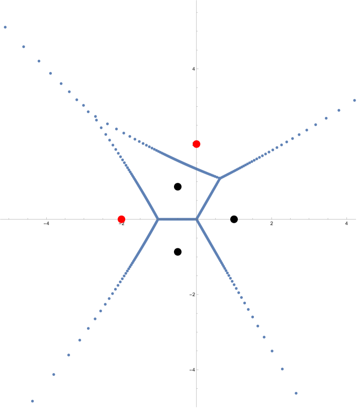
Figure 5. Root distribution of $V_{100}(z)$ for $P=(z+2)(z-2i)$, $Q=z^{3}-1$ and $\ell=3$.

Remark 5.13.

Fig. 5 illustrates the above Example 1. In this case the curve $\Gamma$ is given by $(z^{3}-1)w^{3}=(z+2)(z-2i)$. It is smooth and its projection onto $\mathbb{C}P^{1}_{z}$ has $6$ branching points at the cubic roots of $1$ (shown by black dots in Fig. 5), $-2$ and $2i$ (shown by red dots in Fig. 5), and $\infty$. All of them have multiplicity $2$. The cubic roots of $1$ are also poles of the algebraic function. From Riemann-Hurwitz formula follows that genus of $N\widetilde{\Gamma}$ is $4$. The Voronoi diagram involves only five of the branching points since $\infty$ is a pole of $\omega$.

Example 2. As a concrete special case of the above construction take $\Gamma:=\Gamma_{0}$ as the unit circle given by $z^{2}+w^{2}=1\leftrightarrow w^{2}=1-z^{2}$.

Lemma 5.12 implies the following.

Corollary 5.14.

The curve $\Gamma^{(n)}:=\Gamma_{n}$ is given by the equation

$$w^{2}=-\frac{U^{2}_{n}(z)}{(z^{2}-1)^{2n-1}},$$

where the polynomial sequence $\{U_{n}(z)\}$ is given by the recurrence relation:

$$U_{1}(z)=z;\;U_{n}(z)=(2n-3)zU_{n-1}(z)+(1-z^{2})U^{\prime}_{n-1}(z)\;\text{for \;}n\geq 2.$$

Remark 5.15.

In the latter case the branching points are located at $\pm 1$ and all roots of $U_{n}$ are purely imaginary.

6. Further examples

In the previous sections we discussed the asymptotic root-counting measures of $T_{\omega}^{n}(f)$ which we applied to the study of consecutive derivatives of algebraic functions. Below we provide other types of examples.

6.1. Monomial linear operator applied to a function with one simple pole

Assume that we have a first order linear differential operator of the form $T=R(z)\frac{d}{dz}$ where $R(z)$ is some rational function which we want to apply iteratively to another rational function $f(z)$ and study the asymptotic of the zeros of the iterates. If we can find a change of variable calling the new variable $\phi$ such that $\frac{d}{d\phi}=R(z)\frac{d}{dz}$ then we can in a sense reduce our problem to that about the usual derivative with respect to the variable $\phi$. In fact this procedure corresponds to taking the appropriate Riemann surface defined by $\phi$, its branched covering of $\mathbb{C}P^{1}$ and using Theorem 1.5, see the next example.

For any $\ell\in\mathbb{Z}$, set $T_{\ell}=z^{\ell}\frac{d}{dz}$ and $\omega_{\ell}=z^{-\ell}dz$. Let us calculate the root asymptotic of the sequence $\{T_{\ell}^{n}\left(-\frac{1}{z+a}\right)\}$ with $a\neq 0$ when $n\to\infty$.

Theorem 1.5 in the case under consideration claims the following. For any $\ell\geq 2$, $\omega=\frac{dz}{z^{\ell}}=d\phi$ where $\phi=\frac{z^{1-\ell}}{1-\ell}$. The principal polar locus $\mathcal{PPL}(\omega,\frac{1}{z+a})$ is $\{{-a,\infty\}}$. The image of the Voronoi diagram under $\phi$ is the midline of $[\phi(\infty),\phi(-a)]$. It is a straight line $L$ parametrised by $t\mapsto(\frac{1}{2}+it)\phi(-a)$ (where $t\in\mathbb{R}$).

The inverse image of line $L$ under ramified cover $\phi$ is a planar algebraic curve of equation $\operatorname{Re}(\frac{z}{a})^{\ell-1}=\frac{(-1)^{\ell-1}}{2}$. It is a curve formed by $\ell-1$ loops attached to $0$ each contained in a cone of angle $\frac{2\pi}{\ell-1}$. The limit set $\mathcal{L}(T,\frac{1}{z+a})$ is the branch of the curve contained in the cone containing $-a$. An illustration of the above root distribution can be found in Fig. 6. (The explicit formula for the lemniscate is obtained from the above equation by using $\ell=4$ and $a=1$).

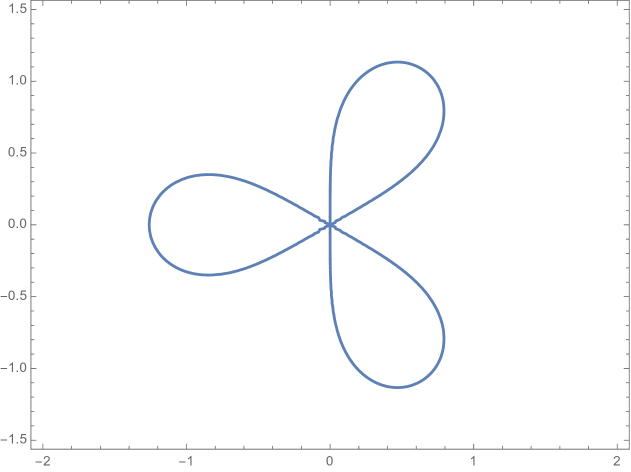
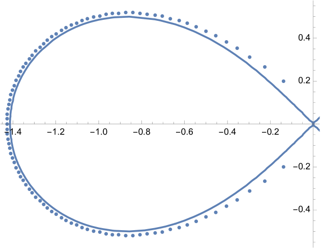
Figure 6. The lemniscate $x^{6}+3x^{4}y^{2}+3x^{2}y^{4}+y^{6}+2x^{3}-6xy^{2}=0$ (left) and its oval together with the roots of $T_{4}^{65}\left(-\frac{1}{z+1}\right)$ (right).

From the latter example it is not difficult to derive the asymptotic root distribution of $T_{\ell}^{n}\left(\sum_{j}\frac{\alpha_{j}}{z-z_{j}}\right)$ when $n\to\infty$.

6.2. Examples in genus one

In the complex plane $\mathbb{C}$, we consider the lattice $\Lambda=\mathbb{Z}+\tau\mathbb{Z}$, where $\tau=\exp(\pi i/3)$. Let $X=\mathbb{C}/\Lambda$ be the associated elliptic curve.

1. Let $\omega=dz$ be the holomorphic 1-form and let $\wp(z)$ be the Weierstraß elliptic function on $X$, where $z$ is the coordinate on $\mathbb{C}$. Since $f$ has one pole of order 2 at 0 and $\omega$ has neither zeros nor poles, the principal polar locus $\mathcal{PPL}(T_{\omega},\wp)$ in $X$ is $\{0\}$. Using the primitive $\phi(z)=z$ of $\omega$, it is easy to see that the Voronoi diagram in $X$ is the quotient by $\Lambda$ of the usual Voronoi diagram on $\mathbb{C}$ determined by the points in $\Lambda$, see Figure 7.

2. For a more complicated example, we consider the derivative of the Weierstraß elliptic function on $X$, which we denote by $\wp_{z}$. Let $\omega=\wp_{z}(z)dz$ be the meromorphic 1-form and $f(z)=\wp_{z}(z)$ be the meromorphic function on $X$. It is a standard fact that $\frac{1}{2},\frac{\tau}{2},\frac{1+\tau}{2}$ are the three simple zeros of $\omega$ in $X$. These points become poles of $T_{\omega}^{n}(f)$ for all $n\geq 1$, so $f$ is not locally factorised by a primitive of $\omega$ there by Lemma 2.1. Hence, they belong to $\mathcal{PPL}(T_{\omega},f)$. Moreover, since the poles of $\omega$ and $f$ are the same, we have that $\mathcal{PPL}(T_{\omega},f)$ is $\{\frac{1}{2},\frac{\tau}{2},\frac{1+\tau}{2}\}$.

   The limit set $\mathcal{L}(T_{\omega},f)$ on $X$ is the preimage under the ramified cover $\wp$ of the Voronoi diagram in the $\mathbb{C}$-plane determined by $\wp(\mathcal{PPL}(T_{\omega},f))$, where the ramification points are precisely the points in $\mathcal{PPL}(T_{\omega},f)$, see Figure 8.

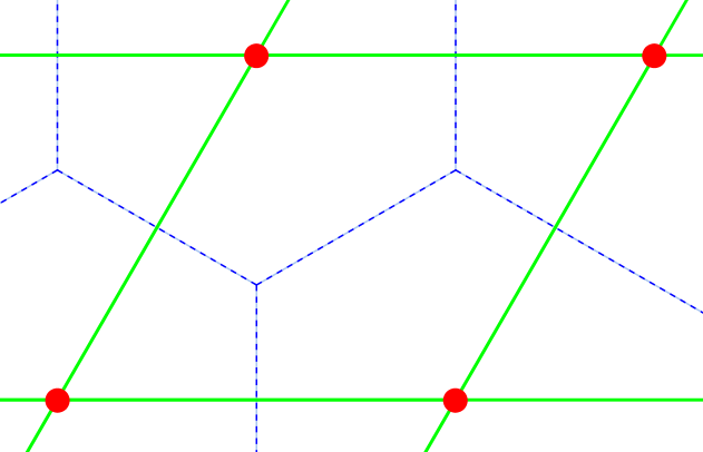
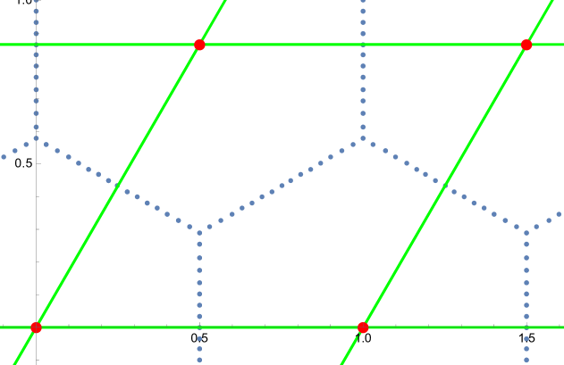
Figure 7. Let $\Lambda=\mathbb{Z}+e^{\frac{i\pi}{3}}\mathbb{Z}$. Left: The Voronoi diagram determined by the poles of $\wp(z)$ (red dots) consists of the blue dashed lines. Right: The zeros of $\wp^{(45)}$ are in blue dots. In this case, parallelograms cut out by the green lines are fundamental domains of the action of $\Lambda$ on $\mathbb{C}$.

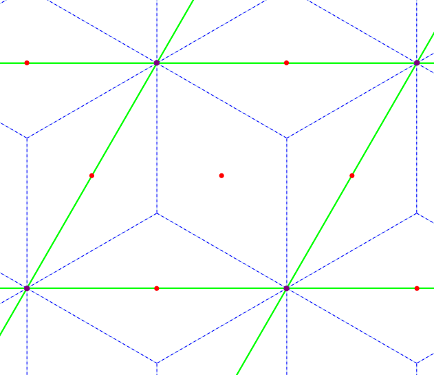
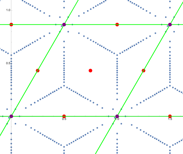
Figure 8. Let $\Lambda=\mathbb{Z}+e^{\frac{i\pi}{3}}\mathbb{Z}$. Left: The red dots are the points of $\mathcal{PPL}(\omega,f)$ where $\omega=\wp_{z}(z)dz$ and $f(z)=\wp_{z}(z)$, which determine the Voronoi diagram in blue dashes. The green lines cut out fundamental domains of the action of $\Lambda$ on $\mathbb{C}$. Right: The dark blue dots are the zeros of $T_{\omega}^{25}(f)$.

7. Outlook

1. (Open Riemann surfaces) The original shire theorem deals with $\mathbb{C}$ which is open and meromorphic functions on it. In particular, the main result of [8] shows that for an entire function of the form $R(z)e^{U(z)}$ with polynomial $U$ a certain part of the total mass of the limiting root-counting measure will be placed at $\infty$. In the present paper we only consider compact Riemann surface $X$, but appropriate modifications of our results work in broader settings.

The crucial hypothesis underlying the constructions of Section 2 is that our translation surfaces are metrically complete. It follows that the first part of Theorem 1.5 still holds for the class of meromorphic functions defined on the surface $X^{\ast}$ punctured at the poles of $\omega$ (and having possibly essential singularities there). The latter class includes the functions studied by Ch. Hägg in [8], that globally have a finite number of zeros and whose asymptotic zero counting measure converges.

If the second part of the theorem is reformulated in the following way, then it also will hold for the class of meromorphic functions defined on the surface $X^{\ast}$. Let $U$ be a relatively compact set in $X^{\ast}$, and let $\mu_{n}(f,U):=\frac{1}{|Z(n,U)|}\sum_{z\in Z(n,U)}\delta_{z}$, where $Z(n,U)$ is the set of zeros of $T_{\omega}^{n}f$ in $U$. This is a probability measure, since $Z(n,U)$ is compact and $f$ meromorphic. The reformulation of the theorem is then that $\mu_{n}(f,U)$ will converge to the right hand side of

$$\mu_{\omega,f}+\sum\limits_{p\in\mathcal{P}}(d_{p}-1)\delta_{p},$$

normalised to a probability measure with support in $U$ in the same manner. Then this reformulation covers [8] as well and gives a more conceptual proof of similar results for meromorphic functions in the plane in [6].

2. (Global geometry of translation surfaces) An essential feature of the theory of translation surfaces is that the same objects have a complex-analytic side (a Riemann surface with a holomorphic differential) and a geometric side (a polygon with pairs of sides identified by translations). Although these two descriptions are theoretically equivalent, going from one side to another is a delicate question in practice.

In a translation surface obtained by the gluing of a family of triangles, the lengths and the slopes of the edges are respectively the module and the argument of the periods of some differential over the corresponding relative homology classes. However, starting with a complex structure (defined by a Fuchsian group for example) and an explicit holomorphic differential (in terms of modular forms), it is a difficult problem to determine which relative homology classes are represented by simple geodesic segments (in order to construct a triangulation).

In the current state of the art, the standard approach to obtain a geometric presentation of a translation surface is to discretise the circle of directions and integrate the differential equation corresponding to the differential form to find saddle connections.

If we can call the latter approach “classical”, Theorem 1.5 suggests a “quantum” way from the complex-analytic data to the flat picture. For a given translation surface $(X,\omega)$, we consider a meromorphic function $f$ with poles located at the zeros of $\omega$. As $n\rightarrow+\infty$, zeros of $T_{\omega}^{n}(f)$ accumulate on the Voronoi diagram defined with respect to the zeros of $\omega$. After an adequate number of iterations, the relative homology classes of the edges of the Delaunay polygonation (dual to the edges of the Voronoi tessellation) are characterised with an arbitrarily low error rate. In Figure 8, the Voronoi diagram of a nontrivial flat metric in genus one is obtained numerically using this very method.

3. (Fuchsian meromorphic connections) generalisation to an even broader settings can be made as follows. Let $X$ be a compact Riemann surface with a Fuchsian meromorphic connection $\nabla$ on a line bundle $\mathcal{L}$. We can investigate the limit set of a global meromorphic section of $\mathcal{L}$ under iteration of $\nabla$.

Fuchsian meromorphic connections induce complex affine structures (see [14]) providing local coordinates where $\nabla$ is conjugated with $\frac{d}{dz}$. We still have a meaningful notion of affine disk immersion so Voronoi diagrams can be defined. Besides, the definition of Cauchy measures in terms of angles is suitable for a generalisation to complex affine structures (see Section 2.5). Nevertheless, an important difference with the current settings is that in most cases, meromorphic connections can fail to be geodesically complete, as in the case of the Hopf torus $\mathbb{C}^{\ast}/\langle z\mapsto 2z\rangle$.

A class of Fuchsian meromorphic connection can already be handled with the methods of the current paper. A $k$-differential $\omega$ is a global meromorphic section of the $k^{th}$ tensor power $K_{X}^{\otimes k}$ of the canonical bundle. In local coordinates, it is a complex analytic object of the form $h(z)dz^{k}$ where $h$ is a meromorphic function. A $k^{th}$ root $\omega^{1/k}$ of $\omega$ can be thought as a global meromorphic section of a line bundle twisted by some character $\chi$ valued in the complex multiplicative group $(\mathbb{C}^{\ast},\times)$. Operator $T:f\mapsto\frac{df}{\omega^{1/k}}$ acting on the space of global sections of a suitable line bundle coincides with a Fuchsian meromorphic connection.

For a compact Riemann surface $X$ with a $k$-differential $\omega$, the canonical $k$-cover (see [1] for details) is the smallest ramified cover $\pi:(\tilde{X},\tilde{\omega})\rightarrow(X,\omega)$ such that $\omega$ is the $k^{th}$ power of a globally defined meromorphic $1$-form. This way, the limit set associated with operator $T$ and some meromorphic section $f$ of a line bundle $\mathcal{L}$ is the projection of the limit set associated with an operator $T_{\tilde{\omega}^{1/k}}$ and a section of $\pi^{\ast}\mathcal{L}$ defined on a surface of higher genus $\tilde{X}$. The latter limit set is described in Theorem 1.5.

Appendix A

A.1. Extending a result of A. G. Orlov

In [15, Theorem 1], A. G. Orlov proved pointwise asymptotics for the coefficients of a Taylor series representation of a branch of an algebraic function, which extends as Puiseux series at singularities. In Theorem A.1 and Corollary A.2 below, we will modify his proof to obtain the uniform convergence for an arbitrary holomorphic function with one Puiseux-type singularity. This is crucial in Section 3, especially in the proof of Lemma 3.2. To make the paper self-contained, we include below a slight modification of Orlov’s original proof.

We denote by $D(x,r)$ the open disk of radius $r>0$ centered at $x\in\mathbb{C}$.

Theorem A.1.

Let $f$ be a holomorphic function on an open disk $D(0,\rho)$ with $\nu$ singularities $a_{1},\ldots,a_{\nu}$ such that $|a_{s}|=\rho$ for $s=1,\ldots,\nu$. Suppose that $f$ extends as a Puiseux series to each singular point and holomorphically to every other point of the circle of radius $\rho$. Then,

$$\frac{f^{(k)}(0)}{k!}\sim\sum\limits_{s=1}^{\nu}\tilde{b}_{s}(k)a_{s}^{-k}+O((\rho+\epsilon)^{-k}$$ (A.1)

where $\epsilon>0$ and, for each $s=1,\ldots,\nu$, the term $\tilde{b}_{s}(k)$ is of the form

$$\tilde{b}_{s}(k)=\frac{B_{s}}{\Gamma(-m_{s})}a_{s}^{m_{s}}k^{-(m_{s}+1)}+o(k^{-(m_{s}+1)}),$$

where $B_{s}$ and $m_{s}$ come from the term $B_{s}(a_{s}-z)^{m_{s}}$ with $m_{s}$ being the smallest number between the least negative exponent or the least non-integer positive exponent in the Puiseux representation of $f$ at $a_{s}$.

Proof.

Using Cauchy’s integral formula, we have:

$$g(k):=\frac{f^{(k)}(0)}{k!}=\frac{1}{2i\pi}\int_{C}\frac{f(u)}{u^{k+1}}du,$$ (A.2)

where $C$ is the positively oriented circle of radius $0<r<\rho$ centered at $0$.

We will change the contour $C$ of this integration to $\gamma$ defined as in Figure 9. In other words, the contour $\gamma$ is the boundary $\partial D$ of the domain $D=D(0,\rho+\epsilon)\setminus\bigcup\limits_{s=1}^{\nu}D(a_{s},\epsilon)$ for a choice of $\epsilon>0$ such that the only singularities of $f$ in $D(0,{\rho+\epsilon})$ are $a_{1},\ldots,a_{\nu}$.

Figure 9. The contour $\alpha$ in Equation (A.2) can be replaced by $\gamma_{0}\cup\bigcup_{s=1}^{\nu}\gamma_{s}$. (The figure displays the case $\nu=4$). On the left, the singularities $a_{1},\ldots,a_{4}$ lie on the circle $|u|=\rho$, and $f$ has no other singularities in $D(0,\rho+\epsilon)$. On the right, the new contour of the integration is the union $\gamma:=\gamma_{0}\cup\gamma_{1}\cup\cdots\cup\gamma_{4}$. The cuts $\sigma_{s}$ are the straight segments joining $a_{s}$ with $\frac{\rho+\epsilon}{\rho}a_{s}$.

Without loss of generality, we assume that the $a_{s}$’s are labeled counterclockwise. Then, the new contour $\gamma$ decomposes into $\gamma_{0}\cup\bigcup_{s=1}^{\nu}\gamma_{s}$ as follows

• $\gamma_{s}$ is the boundary of $D({a_{s},\epsilon})$ for $s=1,\ldots,\nu$;

• $\gamma_{0}$ is the union of the $\nu$ circular arcs of radius $\rho+\epsilon$ between the points $\frac{\rho+\epsilon}{\rho}a_{s}$ and $\frac{\rho+\epsilon}{\rho}a_{s+1}$, where the subscripts are considered modulo $\nu$.

On $\gamma_{0}$, we have $\left|\frac{f(u)}{u^{k+1}}\right|\leq\frac{K}{(\rho+\epsilon)^{k+1}}$, where $K$ is some constant. Thus,

$$g(k)=\frac{1}{2i\pi}\sum\limits_{s=1}^{\nu}\int\limits_{\gamma_{s}}\frac{f(u)}{u^{k+1}}du+O((\rho+\epsilon)^{-k}).$$ (A.3)

For $1\leq s\leq\nu$, we introduce $h_{s}(u)$ which is the Puiseux series of $f$ at $a_{s}$ restricted to the (finitely many) terms with negative exponents. Define $h(u)=\sum\limits_{s=1}^{\nu}h_{s}(u)$ and take $F(u)=f(u)-h(u)$.

Denoting by $\sigma_{s}$ the straight segment joining $a_{s}$ to $\frac{\rho+\epsilon}{\rho}a_{s}$, we have that $h$ and $F$ are holomorphic functions on $D(0,\rho+\epsilon)\setminus\bigcup\limits_{s=1}^{\nu}\sigma_{s}$. Thus, to determine the asymptotic of $g(k)$ as in (A.3), we will study the asymptotic behaviors of the Taylor series coefficients of $h$ and $F$.

In the rest of the proof, $m$ will denote an arbitrary exponent of one of the considered Puiseux series. In other words, $m$ will be an integer multiple of $\frac{1}{M}$, where $M$ is the least common denominator of the exponents of the Puiseux series at the points $a_{1},\dots,a_{s}$.

Writing $h_{s}(u)$ as a (finite) sum $\sum\limits_{m<0}c_{s,m}(a_{s}-u)^{m}$, with $m^{-}_{s}$ being the least exponent, we can use the $\Gamma$ function to express

$$b_{s}(k):=\frac{h_{s}^{(k)}(0)}{k!}$$

explicitly as

$$b_{s}(k) =\sum\limits_{m<0}\frac{1}{k!}c_{s,m}(-1)^{k}(m\cdot(m-1)\cdot\ldots\cdot(m-(k-1))a_{s}^{m-k}$$

$$=\sum\limits_{m<0}\frac{c_{s,m}}{\Gamma(k+1)}\frac{\Gamma(k-m)}{\Gamma(-m)}a_{s}^{m-k}.$$

Using the property $\lim\limits_{k\to+\infty}k^{m+1}\frac{\Gamma(k-m)}{\Gamma(k+1)}=1$ of the $\Gamma$ function, we represent $b_{s}(k)$ asymptotically by the following Puiseux series

$$b_{s}(k)\sim\sum\limits_{m<0}\frac{c_{s,m}}{\Gamma(-m)}k^{-(m+1)}a_{s}^{m-k},$$ (A.4)

whose term with the least exponent equals

$$\frac{c_{s,m^{-}_{s}}}{\Gamma(-m^{-}_{s})}k^{-(m^{-}_{s}+1)}a_{s}^{m^{-}_{s}-k}.$$

Next, to compute the contour integral $G_{s}(k):=\frac{1}{2i\pi}\int\limits_{\gamma_{s}}\frac{F(u)}{u^{k}}du$, we can replace the contour $\gamma_{s}$ by $\sigma^{+}_{s}\cup\sigma^{-}_{s}$, where both $\sigma^{+}_{s}$ and $\sigma^{-}_{s}$ traverse along $\sigma_{s}$ but with opposite orientations. Then, in $D(a_{s},\epsilon)$, writing

$$F(u)=\sum\limits_{s=1}^{\nu}\sum\limits_{m\geq 0}d_{s,m}(a_{s}-u)^{m},$$ (A.5)

we have

$$\frac{1}{2i\pi}\int\limits_{\gamma_{s}}\frac{F(u)}{u^{k+1}}du =\sum_{m\geq 0}\frac{1-e^{2i\pi m}}{2i\pi}d_{s,m}\int\limits_{\sigma^{+}_{s}}\frac{(a_{s}-u)^{m}}{u^{k+1}}du.$$

We note that the integral in the right-hand side is zero if $m$ is a positive integer. One can rewrite the integrand as

$$\frac{(a_{s}-u)^{m}}{u^{k+1}} =a_{s}^{m-(k+1)}\left(1-\frac{u}{a_{s}}\right)^{m}\exp\left(-(k+1)\ln\left(\frac{u}{a_{s}}\right)\right)$$

and, with the change of variable $t=\frac{u}{a_{s}}-1$, one has

$$\frac{1}{2i\pi}\int\limits_{\gamma_{s}}\frac{(a_{s}-u)^{m}}{u^{k+1}}du=\frac{1-e^{2i\pi m}}{2i\pi}e^{-i\pi m}a_{s}^{m-k}\int\limits_{t=0}^{\delta}t^{m}e^{-(k+1)\ln(1+t)}dt$$

where $\delta=\frac{\epsilon}{\rho}$. If we once again change the variable $x=\ln(1+t)$, the problem reduces to the study of the integrals of the form

$$I_{\alpha}(k):=\int_{0}^{\delta_{0}}x^{\alpha}\varphi_{\alpha}(x)e^{-kx}dx,$$

where $\delta_{0}=\ln(1+\delta)$ and $\varphi_{\alpha}(x)=\left(\frac{e^{x}-1}{x}\right)^{\alpha}$. Since $\varphi(x)$ is analytic at $x=0$, an application of Watson’s Lemma yields

$$I_{\alpha}(k)\sim\sum_{n\geq 0}\frac{\varphi_{\alpha}^{(n)}(0)}{n!}\frac{\Gamma(\alpha+n+1)}{k^{\alpha+n+1}}$$

as $k$ tends to $+\infty$ and so $\frac{1}{2i\pi}\int\limits_{\gamma_{s}}\frac{F(u)}{u^{k}}du$ is equivalent to

$$\sum\limits_{m\geq 0}\frac{1-e^{2i\pi m}}{2i\pi}{e^{-i\pi m}}d_{s,m}a_{s}^{m-k}\sum_{n\geq 0}\left(\frac{\varphi_{m}^{n}(0)}{n!}\frac{\Gamma(m+n+1)}{k^{m+n+1}}\right).$$

From the identities $\Gamma(z)\Gamma(1-z)=\frac{\pi}{\sin(\pi z)}$ and

$$\frac{1-e^{2i\pi m}}{2i\pi} =\frac{e^{i\pi m}(e^{-i\pi m}-e^{i\pi m})}{2i\pi}=-e^{i\pi m}\frac{\sin\pi m}{\pi},$$

we deduce that

$$\frac{1-e^{2i\pi m}}{2i\pi}{e^{-i\pi m}}\Gamma(m+n+1) =\frac{{-}\sin(\pi m)}{\Gamma(-m-n)\sin\left[\pi(m+n+1)\right]}$$

$$=\frac{-(-1)^{n+1}}{\Gamma(-m-n)}.$$

After simplification, we obtain that $G_{s}(k)$ is asymptotic to

$$\sum\limits_{m\geq 0}d_{s,m}a_{s}^{m-k}\sum_{n\geq 0}\left(\frac{\varphi_{\alpha}^{n}(0)}{n!}\frac{(-1)^{n}}{\Gamma(-m-n)k^{m+n+1}}\right)$$

as $k$ tends to $+\infty$.

Summing over all contours $\gamma_{1},\dots,\gamma_{\nu}$, and reorganizing the latter series, we obtain that $G(k):=G_{1}(k)+\cdots+G_{\nu}(k)$ is asymptotic to

$$\sum\limits_{s=1}^{\nu}\left(\sum\limits_{m,n\geq 0}d_{s,m}a_{s}^{m}\frac{\varphi_{\alpha}^{n}(0)(-1)^{n}}{n!\Gamma(-m-n)}k^{-(m+n+1)}\right)a_{s}^{-k}.$$ (A.6)

Any given value of $m+n+1$ is realised by at most finitely many tuples $(m,n)$ where $n$ is a non-negative integer while $m$ is a non-negative multiple of $\frac{1}{M}$ different from an integer. Therefore, for each $s$, the inner double series can be written as a series indexed by the increasing exponents of $a_{s}$ whose term with with least exponent is

$$\frac{B_{s}}{\Gamma(-m^{+}_{s})}k^{-(m^{+}_{s}+1)}a_{s}^{m^{+}_{s}-k},$$

where $m^{+}_{s}$ is the least fractional exponent of $(u-a_{s})$ in $F(u)$ expressed as in Equation (A.5) and $B_{s}$ is the coefficient of that term.

Since $f(u)=F(u)+h(u)$, we combine the contributions from the holomorphic part and the Puiseux series part and find the following asymptotic representation of (A.3)

$$g(k)\sim\sum\limits_{s=1}^{\nu}\tilde{b}_{s}(k)a_{s}^{-k}+O((\rho+\epsilon)^{-k}),$$ (A.7)

where $\tilde{b}_{s}(k)$ is a Puiseux series in $k$ which is the sum of (A.4) and (A.5). It follows that the asymptotic behavior of the leading term of $\tilde{b}_{s}(k)$ can be given in the form stated the theorem which finishes the proof. ∎

By tweaking Orlov’s proof, we will prove the uniform convergence that is needed for our purposes.

Corollary A.2.

Let $f$ be a holomorphic function on an open disk $D(0,\rho)$ that extends to a Puiseux series at a unique singularity $a$ with $|a|=\rho$ in $D(a,\epsilon^{\prime})$ for some $\epsilon^{\prime}>0$, and holomorphically at every other point of the boundary circle $\partial D(0,\rho)$. Then, there exist $\delta>0$ and $\epsilon>0$ such that the formula

$$\frac{f^{(k)}(z)}{k!}=b(k,z)(a-z)^{-k}+O((|a-z|(1+\epsilon))^{-k}).$$

holds for any $z\in\overline{D}_{\delta}=\overline{D(0,\delta)}$. Here, we have

$$b(k,z)=K(a-z)^{m_{0}}k^{-(m_{0}+1)}(L+O(k^{-\frac{1}{M}}|a-z|^{\frac{1}{M}}))$$

where $K,L\in\mathbb{C}\setminus\{0\}$ and $M\in\mathbb{N}$ are constants depending only on $f$ and $\delta$ while $m_{0}=k_{0}/M$ is the smallest number between the least negative exponent and the exponent of the first non-integer term of the Puiseux series of $f$.

Proof.

We follow the notation and strategy of the proof of the previous theorem. First, suppose that $a$ is a pole of $f$. Then, as in (A.4), the singular part $h(z)=\sum\limits_{m_{0}\leq m<0}c_{m}(a-z)^{m}$ of $f$ has the following asymptotic description of its derivatives

$$\frac{h^{(k)}(z)}{k!} \sim\sum\limits_{m_{0}\leq m<0}\frac{c_{m}}{\Gamma(-m)}k^{-(m+1)}(a-z)^{m-k}$$

$$=(a-z)^{-k}\left[\frac{c_{m_{0}}}{\Gamma(-m_{0})}(a-z)^{m_{0}}k^{-(m_{0}+1)}\left(1+O(k^{-1}|a-z|^{-1})\right)\right]$$

throughout some $\overline{D}_{\delta}$, where $\delta>0$ is chosen so that $a$ is the only singular point of $f$ closest to $\overline{D}_{\delta}$. The $k$-th derivatives of the holomorphic part of $f$ vanish for $k$ large enough, so the expression above is already in the desired form.

We can now assume that $f$ has a pole-free Puiseux series expansion at $z=a$ given by

$$f(z)=\sum_{k\geq k_{0}}c_{k}(a-z)^{\frac{k}{M}}.$$ (A.8)

Again, choose $\delta>0$ such that $a$ is the closest singularity of $f$ to any point in the closed disk $\overline{D}_{\delta}$. Then, take $\alpha>0$ strictly larger than the maximum distance from $z\in\overline{D}_{\delta}$ to $a$. Think of the curve $\gamma$ in Figure 9 as a diagram for the curve $\gamma(z)$, determined by the center $z\neq a$ in $\overline{D}_{\delta}$, and choose $\epsilon(z)=\frac{|z-a|}{\alpha}\epsilon^{\prime}<\epsilon^{\prime}$. Moving the center of $\overline{D}_{\delta}$ changes the cut $\sigma(z)$ as well as $f$ through the analytic continuation across $\sigma(z)$, but the assumption on $f$ implies that the assumptions of the theorem are still valid. In particular, Equation (A.3) writes as

$$\frac{f^{(k)}(z)}{k!}=\frac{1}{2\pi i}\int_{\gamma_{a}(z)}\frac{f(u)}{(u-z)^{k+1}}du+O((|z-a|(1+\epsilon))^{-k})$$ (A.9)

(with $\epsilon:=\epsilon^{\prime}/\alpha)$. Equation A.9 remains true for any $z\in\overline{D}_{\delta}$, and in fact uniformly, since the implicit constant in the principal term is bounded by the maximum value of (the continuations of) $|f|$ to any cut disk $B(z,|z-a|+\epsilon(z)),\ z\in\overline{D}_{\delta}$.

Fixing $z\in\overline{D}_{\delta}$, as in the proof of the theorem, we rewrite the integral

$$I:=\int_{\gamma_{a}(z)}\frac{f(u)}{(u-z)^{k+1}}du=\int_{\sigma_{a}^{+}}\frac{f(u)}{(u-z)^{k+1}}du+\int_{\sigma_{a}^{-}}\frac{f(u)}{(u-z)^{k+1}}du.$$ (A.10)

Parametrising $\sigma_{a}^{+}(z)$ as $u=a+s(a-z)$, $0\leq s\leq\eta$, where $\eta=\epsilon(z)/|a-z|$, we obtain

$$\int_{\sigma_{a}^{+}(z)}\frac{f(u)}{(u-z)^{k+1}}du=\frac{1}{(a-z)^{k}}\int_{0}^{\eta}\frac{f(a+s(a-z))}{(1+s)^{k+1}}ds$$ (A.11)

Changing the variable by setting $1+s=e^{v}$ results in

$$\frac{1}{(a-z)^{k}}\int_{0}^{\eta^{\prime}}f\left(a+(e^{v}-1)(a-z)\right)e^{-kv}dv,$$ (A.12)

where $\eta^{\prime}=\log(1+\eta)>0$.

The Puiseux expansion in (A.8) implies that the function $\tilde{f}(t):=\sum\limits_{k\geq k_{0}}c_{k}t^{k}$ is analytic in a neighbourhood of $t=0$ and $f(z)=\tilde{f}((a-z)^{1/M})$ for a choice of $t=(a-z)^{1/M}$. The function $\tilde{f}$ is just the analytic continuation of $f$ to the cover $t\mapsto t^{M}=a-z$. In particular, the analytic continuation of $f(z)$ = $\tilde{f}((a-z)^{1/M})$ counterclockwise along a circle with center $z=a$ is given by $\tilde{f}(e^{2\pi i/M}(a-z)^{1/M})$.

Consider $\theta(v):=\frac{e^{v}-1}{v}$, which is analytic and non-zero at $v=0$. Then $\theta^{\frac{1}{M}}(v)$ is defined for $|v|<2\pi$ in such a way that it restricts to the $M$-th root which is real and positive for $v\geq 0$ real. Now, define

$$\tilde{g}_{+}(w) :=\tilde{f}\left(w\cdot\theta^{\frac{1}{M}}((w^{M}/(z-a))\right)$$ (A.13)

$$\tilde{g}_{-}(w) :=\tilde{f}\left(e^{\frac{2\pi i}{M}}w\cdot\theta^{\frac{1}{M}}((w^{M}/(z-a))\right).$$ (A.14)

Thus, along $\sigma_{a}^{+}(z)$ we have

$$f(a+(e^{v}-1)(a-z)) =\tilde{f}(((v(z-a))^{\frac{1}{M}}\cdot\theta^{\frac{1}{M}}(v))$$

$$=\tilde{g}_{+}(((z-a)v)^{\frac{1}{M}}),$$ (A.15)

and, similarly, the analytic continuation of $f$ along $\sigma_{a}^{-}(z)$ is

$$f(a+e^{\frac{2\pi i}{M}}(e^{v}-1)(a-z))=\tilde{g}_{-}(((z-a)v)^{\frac{1}{M}}).$$ (A.16)

By setting

$$g(v)=\tilde{g}_{+}(((z-a)v)^{\frac{1}{M}})-\tilde{g}_{-}(((z-a)v)^{\frac{1}{M}}),$$

we can return to the integral $I$ in (A.10). By (A.12), (A.15), and (A.16), it equals

$$I=\frac{1}{(a-z)^{k}}\int_{0}^{\eta^{\prime}}g(v)e^{-kv}dv.$$ (A.17)

Application of Lagrange’s error term to the first-order Maclaurin polynomial of $g(v)$ proves that the inequality

$$|g(v)-(1-e^{2k_{0}\pi i/M})c_{k_{0}}(a-z)^{m_{0}}v^{m_{0}}|\leq|(a-z)v|^{\frac{k_{0}+1}{M}}$$ (A.18)

holds for all $0\leq v\leq\eta^{\prime}$ and $z\in\overline{D}_{\delta}$, where $c_{k_{0}}(a-z)^{m_{0}},m_{0}=\frac{k_{0}}{M}$, is the first non-integer term of the Puiseux series of $f$, and $D$ is an upper bound for $g^{(k_{0}+1)}$ on the segment between $0$ and $\eta^{\prime}$.

By (A.17) and (A.18),

$$|I-(a-z)^{m_{0}-k}\int_{0}^{\eta^{\prime}}c_{k_{0}}v^{m_{0}}e^{-kv}dv|\leq|a-z|^{m_{0}+\frac{1}{M}-k}\int_{0}^{\eta^{\prime}}Dv^{m_{0}+\frac{1}{M}}e^{-kv}dv.$$ (A.19)

Changing the variable to $u=kv$, we obtain

$$|I-k^{-(m_{0}+1)}(a-z)^{m_{0}-k}\int_{0}^{k\eta^{\prime}}c_{k_{0}}u^{m_{0}}e^{-u}du|$$

$$\leq k^{-(m_{0}+\frac{1}{M}+1)}|z-a|^{m_{0}+\frac{1}{M}-k}\int_{0}^{k\eta^{\prime}}Du^{m_{0}+\frac{1}{M}}e^{-u}du.$$ (A.20)

To obtain the desired asymptotic, we apply a standard proof of Watson’s Lemma. Extending the interval of integration of the latter integral to the whole positive half-axis, we have a bound

$$\int_{0}^{k\eta^{\prime}}Du^{m_{0}+\frac{1}{M}}e^{-u}du\leq\int_{0}^{\infty}Du^{m_{0}+\frac{1}{M}}e^{-u}du=D\Gamma(m_{0}+1/M+1).$$

On the other hand, we have

$$\int_{0}^{k\eta^{\prime}}c_{k_{0}}u^{m_{0}}e^{-u}du =c_{k_{0}}\left(\int_{0}^{+\infty}u^{m_{0}}e^{-u}du-\int_{k\eta^{\prime}}^{+\infty}u^{m_{0}}e^{-u}du\right)$$

$$=c_{k_{0}}(\Gamma(m_{0}+1)+O(e^{-k\eta^{\prime}/2}))$$

Here, the above asymptotic term arises as follows. Consider the integral $\int_{k\eta^{\prime}}^{+\infty}u^{m_{0}}e^{-u}du$. Then, there exists $r=r(m_{0})$ such that $u^{m_{0}}e^{-u/2}\leq 1$ for all $u\geq r_{0}$. Hence, if $k\eta^{\prime}\geq r_{0}$,

$$\int_{k\eta^{\prime}}^{+\infty}u^{m_{0}}e^{-u}du\leq\int_{k\eta^{\prime}}^{+\infty}e^{-u/2}du=2e^{-k\eta^{\prime}/2},$$

where $\eta^{\prime}$ is a constant depending on $m_{0}$. Corollary A.2 then follows from (A.1), noting that the term $O(e^{-k\eta^{\prime}/2})$ is negligible compared to the other asymptotic terms. ∎

Remark A.3.

Note that in the above proof $\delta$ was the distance to the nearest singularity. The constants in the asymptotic estimate depend solely on the values of the function and its analytic continuation. Hence in the situation in which we apply this corollary, the estimate of the lemma is valid in the subset of $D(0,\rho)$ that lies in the Voronoi cell associated with $a$ itself. By a compactness argument, it remains valid in any compact subset of an open Voronoi cell (including the singularity).

A.2. Laplacian of a Puiseux series

It is known that the Laplacian of the logarithmic absolute value of a meromorphic function, considered as a $L^{1}_{loc}$-function (and hence a distribution), is in algebraic-geometric terms the divisor of the function expressed in terms of Dirac measures (see Theorem 3.7.8 in [20]). The same holds for a converging Puiseux series, as we show below.

Lemma A.4.

Let $f(z)=\sum\limits_{k\geq r}a_{k}z^{\frac{k}{m}}$ be a converging Puiseux series where $a_{r}\neq 0$. Then, in some cut disc $U:=D(0,R)\setminus[-R,0]$, we have the following equality of $L^{1}_{loc}$-functions:

$$\frac{2}{\pi}\frac{\partial^{2}}{\partial\bar{z}\partial z}\log|f|=\frac{r}{k}\delta_{0}.$$

Proof.

Writing $f(z)=z^{r/k}g(z)$, we have $\log|f|=\log|g(z)|+\frac{r}{k}\log|z|$, so it suffices to check that $\frac{\partial^{2}\log|g(z)|}{\partial\bar{z}\partial z}$ vanishes as a distribution.

Let $\psi$ be a test function. Since $g(0)\neq 0$, there exists $M>0$ such $M$ is greater than $|\log|g(z)||\cdot|\frac{\partial^{2}\psi}{\partial\bar{z}\partial z}|$ in the (cut) disc.

For an arbitrary $\eta>0$, we introduce the strip $C(\eta)$ characterised by the inequalities $\operatorname{Re}z\leq\eta$ and $-\eta\leq\operatorname{Im}z\leq\eta$. Then, we subdivide the integral

$$\int\limits_{U}\frac{\partial^{2}\log|g(z)|}{\partial\bar{z}\partial z}\psi(z)\,dz\wedge d\bar{z}$$

into the integral over $U\setminus C(\eta)$, which vanishes, since $\log|g|$ is harmonic in this set, and the integral over $U\cap C(\eta)$. Since the absolute value of

$$\int\limits_{U\cap C(\eta)}\frac{\partial^{2}\log|g(z)|}{\partial\bar{z}\partial z}\psi(z)\,dz\wedge d\bar{z}=-\int\limits_{U\cap C(\eta)}\log|g(z)|\frac{\partial^{2}\psi(z)}{\partial\bar{z}\partial z}\,dz\wedge d\bar{z}$$

is bounded by $2M\eta(R+\eta)$ for any $\eta>0$, this integral also has to vanish. Thus,

$$\int\limits_{U}\frac{\partial^{2}\log|g(z)|}{\partial\bar{z}\partial z}\psi(z)dz\wedge\bar{dz}=0$$

for any test function $\psi$. The claim follows. ∎

References

- [1] M. Bainbridge, D. Chen, Q. Gendron, S. Grushevsky, M. Möller. Strata of -differentials. Algebraic Geometry, Volume 6, Issue 2, 196–233, 2019.
- [2] R. Bøgvad and Ch. Hägg. A refinement for rational functions of Pólya’s method to construct Voronoi Diagram. Journal of Mathematical Analysis and Applications, Volume 452, Issue 1, 312-334, 2017.
- [3] C. Boissy, Connected components of the strata of the moduli space of meromorphic differentials. Comment. Math. Helv., Volume 90, Issue 2, 255-286, 2015.
- [4] N. G. Chebotarev. Teoriya Algebraičeskih Funkcii. (Theory of Algebraic Functions), OGIZ, Moscow-Leningrad, 1948.
- [5] J. G. Clunie and A. Edrei. Zeros of successive derivatives of analytic functions having a single essential singularity. J. Anal. Math., Volume 56, 141-185, 1991.
- [6] R. M. Gethner. On the zeros of the derivatives of some entire functions of finite order. Proc. Edinburgh Math. Soc., Volume 28, 381-407, 1985.
- [7] R. M. Gethner. Zeros of the successive derivatives of Hadamard gap series in the unit disk. Michigan Math. J., Volume 36, 403, 1989.
- [8] Ch. Hägg. The asymptotic zero-counting measure of iterated derivatives of a class of meromorphic functions. Arkiv för Matematik, Volume 57, Number 1, 107-120, 2019.
- [9] W. K. Hayman. Meromorphic Functions, Clarendon Press, Oxford, 1964.
- [10] L. Hillairet. Spectral theory of translation surfaces: a short introduction. Sémin. Théor. Spectr. Géom., Vol.28, 51-62,2010.
- [11] V. Keo. generalisation of Plya’s Theorem for Voronoi Diagram Construction, Master Thesis, Royal University of Phnom Penh, 2021.
- [12] A. Kokotov. Polyhedral surfaces and determinant of Laplacian. Proceedings of the American Mathematical Society, Volume 141, Number 2, 725-735, 2013.
- [13] B. Ya. Levin. Lectures on entire functions, Translations of Mathematical Monographs vol.150, American Mathematical Society, Providence, RI, 1996.
- [14] D. Novikov, B. Shapiro, and G. Tahar. On Limit Sets for Geodesics of Meromorphic Connections. J. Dyn. Control Syst., Volume 29, 55-70, 2023.
- [15] A. G. Orlov. On asymptotic behavior of the Taylor coefficients of algebraic functions. Sib. Math. J., Volume 35, 1002-1013, 1994.
- [16] G. Pólya. Ueber die Nullstellen sukzessiver Derivierten. Math. Zeit., Volume 12, 36-60, 1922.
- [17] G. Pólya. On the zeros of the derivatives of a function and its analytic character. Bulletin of the AMS, Volume 49, Issue 3, 178-191, 1943.
- [18] C. L Prather and J. K. Shaw. Zeros of Successive Derivatives of Functions Analytic in a neighbourhood of a Single Pole. Michigan Math. J., Volume 29, 111-119, 1982.
- [19] C. L Prather and J. K. Shaw. A Shire Theorem for Functions with Algebraic Singularities. Internat. J. Math. Math. Sci., Volume 5, no. 4, 691-706, 1982.
- [20] T. Ransford. Potential Theory in the Complex Plane, Cambridge University Press, Cambridge 1995.
- [21] M. G. Robert. A Pólya shire theorem for entire functions, PhD thesis, University of Wisconsin-Madison, 1982.
- [22] E. C. Titchmarsh. The theory of functions, 2nd ed., Oxford University Press, Oxford, 1939.
- [23] M. Troyanov. Les surfaces euclidiennes à singularités coniques. Enseign. Math., Volume 32, 79-94, 1986.
- [24] R. J. Walker. Algebraic curves, Springer-Verlag, New York-Heidelberg, 1978, Reprint of the 1950 edition.
- [25] M. Weiss. Pólya’s Shire Theorem for Automorphic Functions. Geometriae Dedicata, Volume 100, 85-92, 2003.
- [26] J. M. Whittaker. Interpolatory Function Theory, Stechert-Hafner, Inc., New York, 1964
- [27] A. Zeriahi. A Minimum Principle for Plurisubharmonic Functions, Indiana Univ. Math. J., Volume 56, no. 6, 2671-2696, 2007.
- [28] A. Zorich. Flat Surfaces. Frontiers in Number Theory, Physics, and Geometry, Volume 1, 439-585, 2006.