Geometry-Driven Moiré Engineering in Twisted Bilayers of High-Pseudospin Fermions

Abstract

Moiré engineering offers new pathways for manipulating emergent states in twisted layered materials and lattice-mismatched heterostructures. With the key role of the geometry of the underlying lattice in mind, here we introduce the watermill lattice, a two-dimensional structure with low-energy states characterized by massless pseudospin-3/2 fermions with high winding numbers. Its twisted bilayer is shown to exhibit magic angles, where four isolated flat bands emerge around the Fermi level, featuring elevated Wilson-loop windings and enhanced quantum geometric effects, such as an increase in the ratio of the Berezinskii-Kosterlitz-Thouless (BKT) transition temperature to the mean-field critical temperature under a weak Bardeen-Cooper-Schrieffer (BCS) pairing. We discuss how the watermill lattice could be realized in the MXene and group-IV materials. Our study highlights the potential of exploiting lattice geometry in moiré engineering to uncover novel quantum phenomena and tailor emergent electronic properties in materials.

Moiré engineering is drawing intense interest as an innovative technique for manipulating low-dimensional electronic structures by leveraging emergent potentials arising from moiré patterns in twisted-layered materials and lattice-mismatched heterostructures [1, 2, 3, 4]. A remarkable consequence is the emergence of flat electronic bands with substantial quantum metric, which allows the exploration of exotic quantum phenomena, including strongly correlated physics and effects of quantum geometry on physical properties, such as superfluid weights [5, 6, 7, 8, 9] and light-matter interactions [10, 11, 12, 13].

The physics of twisted bilayer systems, such as twisted bilayer graphene (TBG) [4, 14, 15, 16, 17, 5, 18, 19, 20, 21, 22, 23, 24] and transition metal dichalcogenides (TMDs) [25, 26, 27, 28, 29, 30, 31, 32, 33, 34, 35, 36, 37, 38], is driven by the underlying lattice structures and twist angles and the associated intricate moiré patterns. At specific ”magic angles,” flat bands are generated, which enable the exploration of exotic quantum phenomena, such as unconventional superconductivity [39, 18, 19, 20, 21, 22, 23, 28, 29], fractional quantum anomalous Hall effects [30, 31, 32, 33], excitonic physics [34, 35, 36, 37, 38, 40], and complex magnetism [41, 42, 43, 44, 45, 46, 47]. Moiré physics in twisted-bilayer anisotropic lattices can induce stripes and quasi-one-dimensional behaviors, leading to density waves and Luttinger liquid phases [48, 49, 50, 51, 52, 53, 54, 55].

Relatively simple minimalistic models have often sparked breakthroughs in condensed matter physics by stripping away complexity to isolate essential physics and uncover new insights into the nature of quantum matter. Two-dimensional (2D) lattice models, such as the kagome [56, 57, 58], dice [59, 60, 61, 62, 63], Lieb [64, 57, 58] and checkerboard lattices [65, 66] showcase unique lattice geometries that give rise to distinctive quantum geometric phenomena. Effects of quantum geometry become especially enhanced in moiré structures constructed from special 2D lattices.

A recent example is provided by high pseudospin $1$ low-energy states (LESs) in twisted bilayers of Dice lattices which support a tunable number of isolated flat bands near the Fermi level [67, 68]. This naturally prompts the question: What unique behaviors might arise in lattices with LESs characterized by higher pseudospins, such as $3/2$? Accordingly, here we introduce the novel 2D watermill lattice, which hosts pseudospin $3/2$ LESs, and the moiré physics of twisted bilayer watermill lattice. Experimental realizations of the watermill lattice in real materials are also discussed.

The watermill lattice—

Inspired by the Dice lattice, we introduce the watermill lattice. It consists of a honeycomb lattice augmented by a central atom, labeled $A$, which with two orbitals, $A_{1}$ and $A_{2}$. The original honeycomb lattice sites retain their single orbitals, B and C. We focus on the nearest-neighbor hopping interactions within this lattice, with hopping between site A and its neighboring B (C) sites mediated by orbitals $A_{1}$ ($A_{2}$), as depicted in FIG. 1(a).

Figure 1: (a) A schematic diagram of the watermill lattice. Nearest-neighbor hopping between orbitals $B$ and $C$ are marked in blue, and between orbitals $A_{1}(A_{2})$ and orbital $B(C)$ are marked in green (magenta). (b) Band structure of the watermill lattice near the $K,K^{\prime}$-valley.

Note that the atoms at sites $B$ and $C$ are identical, whereas the central atom at site $A$ is distinct. The hopping interactions between pairs of sites $A$-$B(C)$ involve orbitals $A_{1}(A_{2})$ and $B(C)$, respectively. Due to the six-fold rotational symmetry $C_{6z}$, the hopping strengths between $A$-$B$ and $A$-$C$, are equal, denoted as $t^{\prime}$, but differ from those between $B$ and $C$, denoted as $t$. We set $t^{\prime}=\frac{\sqrt{3}}{2}t$. Consequently, in the basis of $\Psi={(A_{1},B,C,A_{2})}^{T}$, the Bloch Hamiltonian can be written as:

$$H_{\text{WM}}(\vec{k})=t\begin{pmatrix}0&\frac{\sqrt{3}}{2}h(\vec{k})&0&0\\ \frac{\sqrt{3}}{2}h(\vec{k})^{*}&0&h(\vec{k})&0\\ 0&h(\vec{k})*&0&\frac{\sqrt{3}}{2}h(\vec{k})\\ 0&0&\frac{\sqrt{3}}{2}h(\vec{k})^{*}&0\end{pmatrix},$$ (1)

where $h(\vec{k})=1+2\cos(\frac{\sqrt{3}k_{x}}{2})e^{-i\frac{3k_{y}}{2}}$.

The watermill lattice, characterized by the hopping parameters outlined above, exhibits time-reversal symmetry (TRS) $\mathcal{T}=\mathcal{K}$, sixfold rotational symmetry $C_{6z}$, chiral symmetry $\Gamma$, particle-hole symmetry $\Xi$, and the combined symmetry $C_{2z}\mathcal{T}$. These symmetries are tied to the lattice structure. For the Hamiltonian in Eq. (1), these symmetries are represented by $\Gamma=\sigma_{0}\otimes\sigma_{3}$, $\Xi=\sigma_{0}\otimes\sigma_{3}\mathcal{K}$, and $C_{2z}\mathcal{T}=\sigma_{1}\otimes\sigma_{1}\mathcal{K}$, where $\mathcal{K}$ is the complex conjugation operator, $\sigma_{1,2,3}$ are Pauli matrices, and $\sigma_{0}$ is the identity matrix.

The watermill lattice exhibits valley structures with four-fold degenerate cones at the $K$ and $K^{\prime}$ points. The low-energy effective Hamiltonian around the valleys in the continuum limit is:

$$H_{0}(\vec{q})=\frac{3t}{2}(q_{x}S_{1}+\xi q_{y}S_{2}).$$ (2)

Here, $\xi=\pm$ designates the valley index, where $\xi=+$ refers to the $K$ valley, and $\xi=-$ to the $K^{\prime}$ valley. $\vec{q}=\vec{k}-K^{(\prime)}$, and $S_{i}$ denote the spin matrices for a spin-3/2 fermion [69]. Equation (2) describes a four-fold degenerate pseudospin-3/2 quasiparticle excitation, protected by the sublattice symmetry at $K$ and $K^{\prime}$ points in the Brillouin zone (BZ). Furthermore, each band exhibits a nontrivial pseudo-spin texture with winding number $w=\xi$, as illustrated in FIG. 1(b).

Twisted bilayer watermill lattice (TBWL)—

We investigate moiré physics of TBWL using continuum models constructed via the Bistritzer-MacDonald formalism [24, 14]

$$H(\theta,\xi)=\begin{pmatrix}H_{R}(\frac{\theta}{2},\xi)&T\\ T^{\dagger}&H_{R}(-\frac{\theta}{2},\xi)\end{pmatrix}.$$ (3)

Here, $\xi$ indicates the monolayer valley degree of freedom, and $\theta$ is the twist angle between the layers. $H_{R}(\theta,\xi)$ denotes the low-energy effective Hamiltonian of the rotated monolayer watermill lattice, which can be obtained via a rotation $\theta$ of the Hamiltonian in Eq. (2)

$$H_{R}(\theta,\xi)=v(q_{x}\hat{x}+\xi q_{y}\hat{y})\cdot\vec{S}^{(\theta)}.$$ (4)

Here, $\vec{S}^{(\theta)}\equiv e^{-i\frac{\theta}{2}S_{3}}\vec{S}e^{i\frac{\theta}{2}S_{3}}$. Vector $\vec{q}=\vec{k}-K_{\xi}^{(\theta)}$, with $K_{\xi}^{(\theta)}$ is the $K$ point of the $\xi$ valley in the rotated monolayer BZ. The interlayer tunneling $T$ takes the matrix form:

$$T=\begin{pmatrix}\omega_{1}g(\vec{r})&\omega_{2}{{}^{\prime}}g(\vec{r}-\vec{r}_{AB})&\omega_{3}g(\vec{r}+\vec{r}_{AB})&\omega_{4}g(\vec{r})\\ \omega_{2}{{}^{\prime}}g(\vec{r}+\vec{r}_{AB})&\omega_{1}g(\vec{r})&\omega_{2}g(\vec{r}-\vec{r}_{AB})&\omega_{3}g(\vec{r}+\vec{r}_{AB})\\ \omega_{3}g(\vec{r}-\vec{r}_{AB})&\omega_{2}g(\vec{r}+\vec{r}_{AB})&\omega_{1}g(\vec{r})&\omega_{2}{{}^{\prime}}g(\vec{r}-\vec{r}_{AB})\\ \omega_{4}g(\vec{r})&\omega_{3}g(\vec{r}-\vec{r}_{AB})&\omega_{2}{{}^{\prime}}g(\vec{r}+\vec{r}_{AB})&\omega_{1}g(\vec{r})\end{pmatrix}.$$ (5)

The interlayer tunneling matrix element $T_{ij}$ describes tunneling from the $j^{\text{th}}$ orbital in the bottom layer to the $i^{\text{th}}$ orbital in the top layer. Here, $g(\vec{r})=\sum_{i}e^{i\vec{q}_{i}\cdot\vec{r}}$, where $\vec{q}_{i}$ are momentum vectors connecting valleys from different layers in the BZ. Specifically, $(\vec{q}_{1},\vec{q}_{2},\vec{q}_{3})=\frac{4\pi}{3L_{s}}(\hat{y},-\frac{\sqrt{3}}{2}\hat{x}-\frac{1}{2}\hat{y},\frac{\sqrt{3}}{2}\hat{x}-\frac{1}{2}\hat{y})$. The coordinate origin is set at the center of the AA-stacked region, as illustrated in FIG. 2(a), with the positions of different stacked regions given by $\vec{r}_{AB}=-\vec{r}_{BA}=\frac{L_{s}}{\sqrt{3}}\hat{x}$. Here, $L_{s}$ is the norm of the translation vector of the moiré cell.

Parameters $\omega_{i}$ represent various interlayer hopping strengths. Specifically, $\omega_{1}$ gives intra-orbital hopping, $\omega_{4}$ is intra-sublattice tunneling between $A_{1}$ and $A_{2}$ orbitals, $\omega_{2}$ is inter-sublattice hopping between $B$ and $C$ orbitals, $\omega_{2}^{\prime}$ gives inter-orbital hopping between $A_{1}$-$B$ and $A_{2}$-$C$ pairs, and $\omega_{3}$ gives hopping between $A_{1}$-$C$ and $A_{2}$-$B$ pairs. Precise values of $\omega_{i}$ depend on the orbital types within each sublattice. For the TBWL with sublattice symmetry, as an example, we consider a configuration where $A_{1}$ and $A_{2}$ orbitals are of $sp_{2}$ type, while $B$ and $C$ orbitals are of $s$ type, preserving the $C_{3z}$ symmetry (FIG. 1). This configuration minimizes the overlap between $A_{1}$ and $A_{2}$ orbitals. This also applies to interlayer bonds (FIG. 2(b)), so that the hopping parameters exhibit the following hierarchy: $\omega_{1}\sim\omega_{2}\sim\omega_{2}^{\prime}\sim\omega_{3}\gg\omega_{4}$.

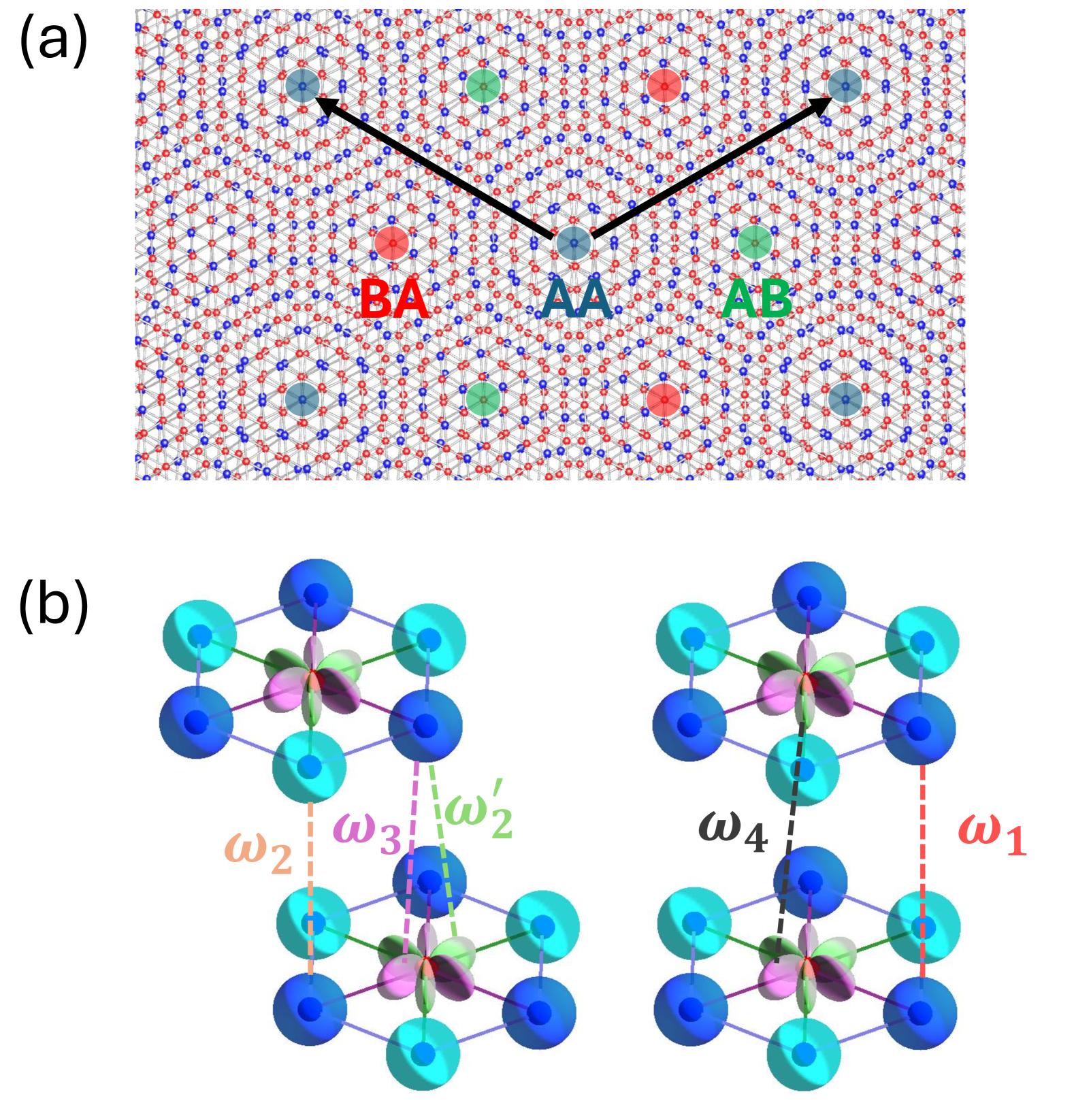
Figure 2: (a) A schematic of the moiré pattern of the twisted bilayer watermill lattice. Colored circles mark the centers of the high-symmetry stacked regions. Black arrows indicate the translation vectors of the moiré unit cell. (b) A schematic for interlayer tunneling in the AB-stacked (left) and AA-stacked (right) regions in the twisted bilayer watermill lattice.

Chiral TBWL—

In the TBWL, we employ a unified hopping scheme for both the inter- and intra-layer interactions, assuming that $\omega_{1}=\omega_{3}=\omega_{4}=0$ and $\omega_{2}{{}^{\prime}}=\frac{\sqrt{3}}{2}\omega_{2}$. This implies that hoppings within pairs $A_{1}$-$B$, $A_{2}$-$C$, and $B$-$C$ occur from the top to the bottom layer in the same way as in the intralayer hopping processes. The preserved symmetries in the monolayer then include chiral symmetry $\Gamma$, particle-hole symmetry $\Xi$, and the combined symmetry $C_{2z}\mathcal{T}$, are also maintained in the TBWL. These symmetries can be represented by the matrices $\Gamma=\tau_{0}\otimes\sigma_{0}\otimes\sigma_{3}$, $C_{2z}\mathcal{T}=\tau_{0}\otimes\sigma_{1}\otimes\sigma_{1}\mathcal{K}$, and $\Xi=\tau_{0}\otimes\sigma_{0}\otimes\sigma_{3}\mathcal{K}$. Here, $\tau_{i}$ are Pauli matrices representing the layer degree of freedom. Moreover, the system is controlled by the dimensionless parameter $\alpha\equiv\frac{\omega_{2}}{vk_{\theta}}$, where $k_{\theta}=2k_{D}\sin(\frac{\theta}{2})$ with $k_{D}$ being the monolayer Dirac momentum [24, 14, 16]. For our calculations, we set $2vk_{D}=19.81$ eV. We, therefore, refer to the TBWL in this limit as chiral TBWL (CTBWL) like the chiral TBG (CTBG) [15].

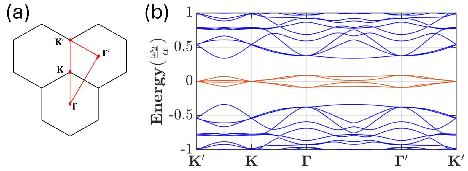
Figure 3: (a) k-path in the moiré Brillouin zone. (b) Twisted bilayer watermill lattice band structure calculated using Eq. (3) with $\alpha=0.5$.

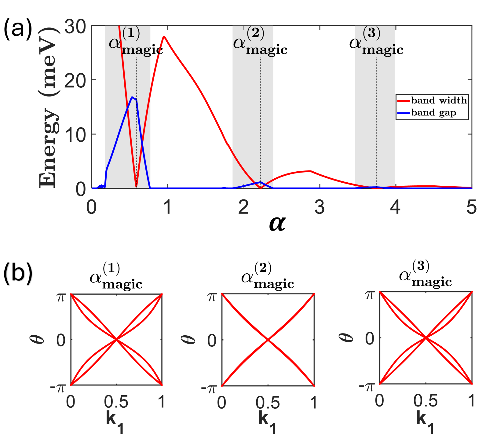
Figure 4: (a) Band gap between the four isolated flat bands near the Fermi level with other high-energy bands (blue) and their bandwidths (red) as a function of $\alpha$. Vertical dashed lines indicate the $i^{\text{th}}$ magic angle, $\alpha_{\text{magic}}^{(i)}$. (b) Wilson loop spectrum of the gapped regions (gray) labeled by the $\alpha_{\text{magic}}^{(i)}$ within.

The electronic structure of CTBWL now features four isolated flat bands near the Fermi level within specific $\alpha$ ranges (FIG. 3). These bands become perfectly flat at certain magic angels, denoted by $\alpha_{\text{magic}}^{(i)}$, with the approximate values of $\alpha_{\text{magic}}^{(1,2,3)}=(0.586,2.222,3.749)$ (FIG. 4(a)). The emergence of these magic angels can be attributed to chiral symmetry and it can be analytically elucidated through the pseudo-Landau level representation [16]; see Supplemental Materials (SM) for details [70].

Quantum geometric effects—

The isolated flat bands in CTBWL have a winding number of $2$ in their Wilson loop spectrum for the first three magic angels (FIG. 4(b)). Symmetry $C_{2z}\mathcal{T}$ ensures that the Wilson loop spectrum is symmetric around $0$, as their Wilson loop operator eigenvalues are complex conjugates [5, 70]. Such a high winding number further implies an enhanced quantum metric of the flat bands [77].

The CTBWL exhibits a significantly larger trace of quantum weight $K$ [6, 5, 78, 79] for its isolated flat bands at magic angels compared to CTBG, where $K\cong 2$ at its first magic angle. In contrast, the values are quantified as $K\cong(6.748,4.844,4.153)$ for the CTBWL at the magic angels $\alpha_{\text{magic}}^{(1,2,3)}$, respectively. We adopt the continuum model for CTBG in [15] and use the same lattice constant and velocity in the calculations for CTBG and CTBWL; see SM for details [70]. The higher trace of quantum weight is crucial for understanding superconducting properties, as this weight is directly related to the corresponding superfluid weight for weak $s$-wave pairing potentials within the BCS mean-field theory [5, 6, 7, 8, 9].

In CTBWL, the superfluid weight is isotropic due to $C_{3z}$ symmetry, allowing for a direct prediction of the BKT transition temperature $T_{\text{BKT}}$ at specific filling factors $\nu$ [80, 5]. Based on the calculated trace of the quantum weight $K$ in CTBWL, $T_{\text{BKT}}$ is estimated to be around $0.771\ T_{\text{MF}}$ at its first magic angle $\alpha_{\text{magic}}^{(1)}$ for $\nu=1/4$. In contrast, the $T_{\text{BKT}}$ of CTBG at its first magic angle with $\nu=1/4$ is only about $0.468\ T_{\text{MF}}$. At the same electron filling, CTBWL hosts more electrons than CTBG due to its four isolated flat bands per spin per valley, compared to CTBG’s two. Moreover, CTBWL exhibits a higher $T_{\text{BKT}}/T_{\text{MF}}$ ratio than CTBG when the number of occupied electrons is fixed at two per moiré cell. In this scenario, CTBWM corresponds to $\nu=1/8$ and $T_{\text{BKT}}=0.733\ T_{\text{MF}}$, see SM for details [70].

Discussion—

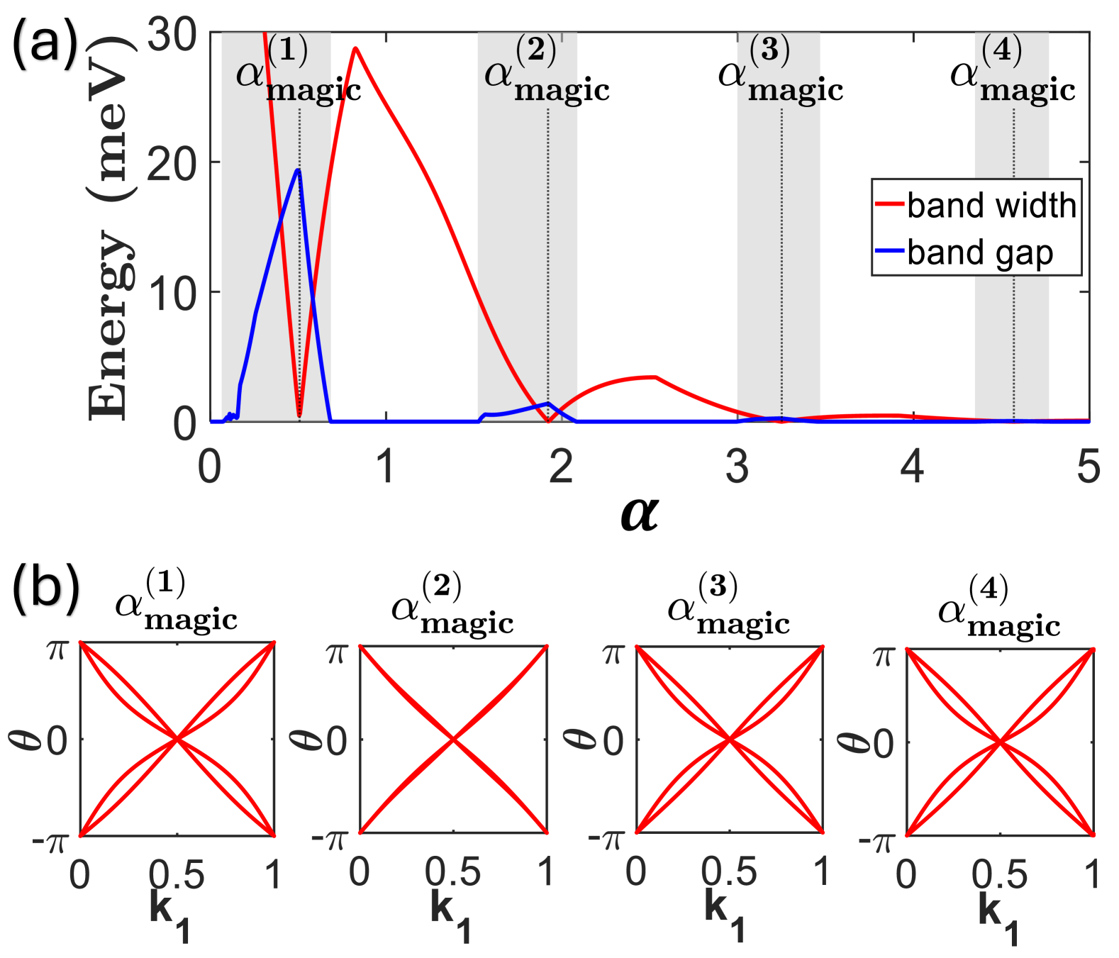
Figure S4: (a) Band gap between the four isolated flat bands near the Fermi level with other high-energy bands (blue) and their bandwidth (red) as a function of $\alpha$ in CTBWL with uniform interlayer tunneling $\omega_{2}{{}^{\prime}}=\omega_{2}$. Vertical dashed lines indicate the $i^{\text{th}}$ magic angle as $\alpha_{\text{magic}}^{(i)}$. The magic angles are: $\alpha_{\text{magic}}^{(1)}\cong 0.508$, $\alpha_{\text{magic}}^{(2)}\cong 1.921$, $\alpha_{\text{magic}}^{(3)}\cong 3.25$, and $\alpha_{\text{magic}}^{(4)}\cong 4.57$. (b) Wilson-loop spectrum of the gapped regions (gray) labeled by the $\alpha_{\text{magic}}^{(i)}$ within.

In the watermill lattice, the symmetry $C_{2z}\mathcal{T}$ is crucial for the hopping structure that gives rise to LESs with a pseudospin-3/2 structure. The four-fold degeneracies at valleys in this lattice are resilient to small modifications in hopping strength as long as $C_{3z}$, $C_{2z}\mathcal{T}$ and the chiral symmetry $\Gamma$ are preserved. The hopping strength between orbitals $B$ and $C$, $t_{BC}$, is $\frac{2}{\sqrt{3}}$ times larger than that between other orbitals, $t_{\text{others}}$. However, varying the ratio between $t_{BC}$ and $t_{\text{others}}$ does not lift the four-fold degeneracy but rather modifies the velocities of the Dirac cones, and the pseudospin texture remains a nontrivial winding pattern around the valleys [70]. Furthermore, magic angels persist in the corresponding CTBWL, see SM and FIG. S4 for details [70]. This robustness in hopping strengths should help realize materials with LESs characterized by a pseudospin-3/2 configuration. A promising candidate is the LaAlO₃/SrTiO₃ (111) quantum well [81]. Other interesting possibilities for engineering the watermill lattice would be utilizing covalent-organic frameworks and metal-organic frameworks [82, 83, 84, 85, 86, 87, 88, 89, 90, 91, 92, 93] or employing CO molecules on Cu(111) surface [94, 95, 96].

The CTBWL retains its magic angles even when subjected to a weak onsite potential difference between the $A$ and $B/C$ sites (FIG. S3(a) [70]), resulting in the four isolated flat bands splitting into two pairs of entangled flat bands separated by a small band gap as detailed in the SM, see FIG. S2(c) [70]. Despite this splitting, the magic angles remain unchanged and the flat bands in each pair continue to exhibit non-trivial windings of their hybrid Wannier centers (FIG. S3(b) [70]). Since the onsite potential difference preserves $C_{2z}\mathcal{T}$ symmetry, these non-trivial windings provide a lower bound for the quantum metric of the two isolated flat bands in each group [5, 77]. These features should help materials realization of the CTBWL.

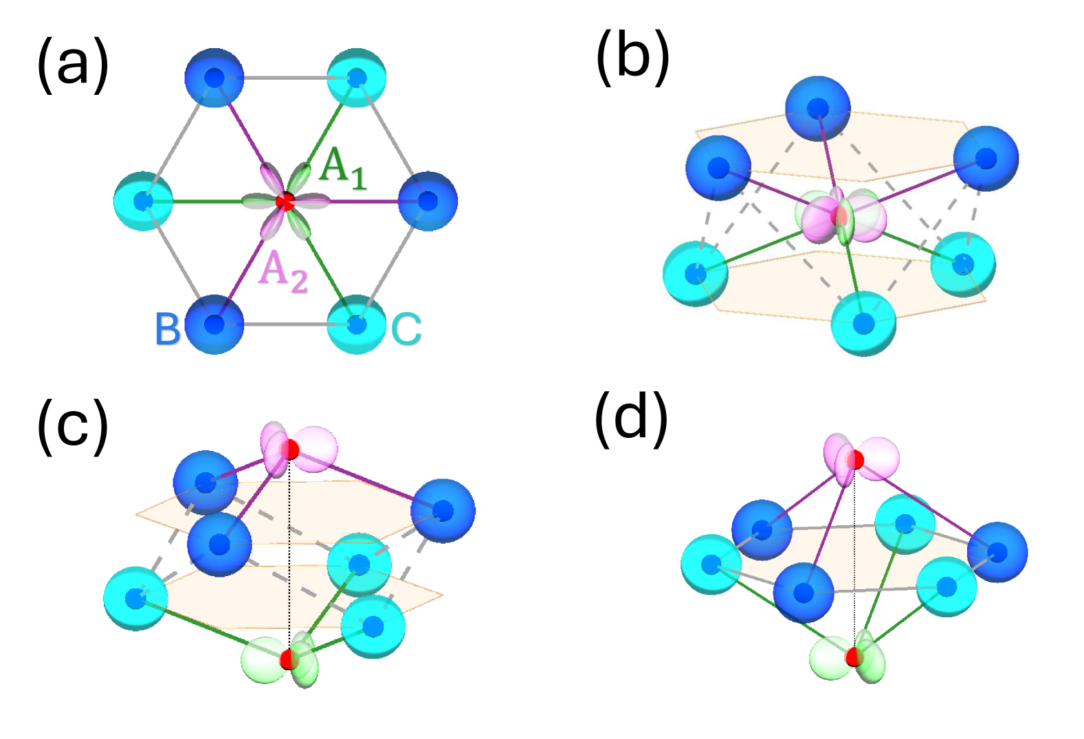
Figure 5: (a) Top view of the modified watermill lattice, where atoms are on different planes but related by the inversion symmetry. (b-d) Side views of the modified watermill lattice with different modifications. Here, orbitals on atoms B and C are assigned distinct colors to emphasize their position differences in these schematic diagrams.

We emphasize that the hopping structure of the watermill lattice can also be reproduced in a modified watermill lattice, where the atoms reside in different planes connected by the inversion symmetry $\mathcal{P}$. Here, $\mathcal{PT}$ symmetry substitutes the $C_{2z}\mathcal{T}$ symmetry in the watermill lattice. This configuration could be achieved, for example, by vertically realigning sites $B$ and $C$ with the separation of $A_{1}$ and $A_{2}$ orbitals (FIG. 5(c)) or by maintaining the $A_{1}$ and $A_{2}$ orbitals in place (FIG. 5(b)). These modifications should be possible to realize in two-dimensional group IV materials such as Germanene and Stanene [97, 98, 99, 100, 101, 102, 103, 104, 105, 106, 107] as well as MXene [108, 109, 110, 111, 112] with B/C and A sites aligning with M and T sites in MXene, respectively. Further studies could seek stable MXene materials or structures with needed orbital arrangements. Separating $A_{1}$ and $A_{2}$ orbitals onto distinct, vertically separated sites (FIG. 5(d)) could also generate the watermill lattice hopping structure. Generally, these modified structures influence the architecture of interlayer tunneling, thus impacting the moiré physics in TBWL, a topic that extends beyond the scope of this study. Our study provides a new pathway for exploring moiré physics via twisted bilayer high pseudospin fermion lattices.

Supplemental Materials: Geometry-Driven Moiré Engineering in Twisted Bilayers of High-Pseudospin Fermions

I S1. Origin of the magic angles in chiral twisted bilayer watermill lattice (CTBWL)

The CTBWL refers to the twisted bilayer watermill lattice (TBWL) that involves only the interlayer tunneling between $A_{1}$-$B$, $A_{2}$-$C$, and $B$-$C$ pairs, which has the chiral symmetry $\Gamma=\tau_{0}\otimes\sigma_{0}\otimes\sigma_{3}$ as noted in the main text. Here, $\tau_{i}$ are Pauli matrices representing the degree of freedom of the layer, and $\sigma_{i}$ are Pauli matrices for the orbital degree of freedom. Then, without loss of generality, we can rewrite Eq. 3 for the $K$ valley of the monolayer BZ in the main text using the basis $\begin{pmatrix}A_{1}^{(\text{top})},&A_{1}^{(\text{bot})},&C^{(\text{top})},&C^{(\text{bot})},&B^{(\text{top})},&B^{(\text{bot})},&A_{2}^{(\text{top})},&A_{2}^{(\text{bot})}\end{pmatrix}^{T}$ to yield [15]:

$$H\propto\begin{pmatrix}0&0&\frac{\sqrt{3}}{2}D(\vec{r})&0\\ 0&0&D^{*}(-\vec{r})&\frac{\sqrt{3}}{2}D(\vec{r})\\ \frac{\sqrt{3}}{2}D^{*}(-\vec{r})&D(\vec{r})&0&0\\ 0&\frac{\sqrt{3}}{2}D^{*}(-\vec{r})&0&0\end{pmatrix}.$$ (S1)

Here, $o^{(\text{top/bot})}$ with $o=A_{1(2)},B,C$ indicates the $o$th orbital on top/bottom layer and,

$$D(\vec{r})=\begin{pmatrix}-i\bar{\partial}&\alpha t(\vec{r})\\ \alpha t(-\vec{r})&-i\bar{\partial}\end{pmatrix},$$ (S2)

where $t(\vec{r})=e^{i\vec{q}_{1}\cdot\vec{r}}+e^{-i\frac{2\pi}{3}}e^{i\vec{q}_{2}\cdot\vec{r}}+e^{i\frac{2\pi}{3}}e^{i\vec{q}_{3}\cdot\vec{r}}$ and $\alpha\equiv\frac{\omega_{2}}{vk_{\theta}}$ are as defined in the main text. Note that we have approximate $\vec{S}^{(\theta)}\cong\vec{S}$ since $\theta\ll 1$ is assumed. The wave function is decomposed into $\Psi(\vec{r})=\begin{pmatrix}\psi_{A_{1}}^{(\vec{k})}(\vec{r}),&\psi_{B}^{(\vec{k})}(\vec{r}),&\psi_{C}^{(\vec{k})}(\vec{r}),&\psi_{A_{2}}^{(\vec{k})}(\vec{r})\end{pmatrix}^{T}$, where $\psi_{o}^{(\vec{k})}(\vec{r})$ with $o=A_{1(2)},B,C$ are two-component spinors indicating the component of the wave functions on $o$th orbitals in both layers at $\vec{k}$ point in the moiré Brillouin zone (MBZ). Then, the existence of exactly-flat bands at the magic angles implies that:

$$\begin{pmatrix}\frac{\sqrt{3}}{2}D(\vec{r})&0\\ D^{*}(-\vec{r})&\frac{\sqrt{3}}{2}D(\vec{r})\end{pmatrix}\begin{pmatrix}\psi_{C}^{(\vec{k})}(\vec{r})\\ \psi_{A_{2}}^{(\vec{k})}(\vec{r})\end{pmatrix}=0.$$ (S3)

We anticipate that the flat-band wave functions at magic angles have the form:

$$\Phi_{1}^{(\vec{k})}(\vec{r})=\begin{pmatrix}\phi_{C}^{(\vec{k})}(\vec{r})\\ 0\\ 0\end{pmatrix}+\begin{pmatrix}0\\ 0\\ \delta\psi_{C}^{(\vec{k})}(\vec{r})\end{pmatrix}\text{ and }\Phi_{2}^{(\vec{k})}(\vec{r})=\begin{pmatrix}0\\ 0\\ \phi_{A_{2}}^{(\vec{k})}(\vec{r})\end{pmatrix},$$ (S4)

where the functions $\phi_{C}^{(\vec{k})}(\vec{r})$ and $\phi_{A_{2}}^{(\vec{k})}(\vec{r})$ satisfy the equations:

$$D(\vec{r})\phi_{C(A_{2})}^{(\vec{k})}(\vec{r})=0.$$ (S5)

Given that the wave functions are represented in the basis $e^{i\vec{q}\cdot\vec{r}}$, where $\vec{q}=\vec{k}-K_{\xi}^{(\theta)}$, with $K_{\xi}^{(\theta)}$ as the $K$ point in the $\xi$ valley of the rotated monolayer (i.e., top or bottom layer) BZ, there exist two zero modes for Eq. (S5) at each valley within the MBZ when $\alpha=0$. As the valleys in the MBZ are $C_{3z}$-symmetric locations, the wave functions at these points are defined by the $C_{3z}$ symmetry eigenvalues. Moreover, because the $C_{3z}$ symmetry commutes with the particle-hole symmetry $\Xi$, each zero mode at each valley can be individually analyzed, where the $C_{3z}$ rotation operator for each spinor can be formulated using $\hat{C}_{3z}=\text{diag}(1,e^{-i\frac{2\pi}{3}})e^{\frac{2\pi}{3}\vec{r}\times\nabla}$ resulting from $D(C_{3z}\vec{r})=e^{i\frac{2\pi}{3}}D(\vec{r})$. Since $\alpha\neq 0$ does not break the symmetries, the zero modes at each valley persist as $\alpha$ is adiabatically turned on [15].

Since zero-modes always exist at $K,K^{\prime}$ points in the MBZ for all $\alpha$ and the kinetic part of $D(\vec{r})$ is antiholomorphic in terms of the complex positions $z=x+iy$ and $\bar{z}=x-iy$, we can construct the flat band wave functions at magic angles using:

$$\Phi_{1}^{(\vec{k})}(\vec{r})=h^{(\vec{k})}(z)\begin{pmatrix}\phi_{C}^{(K)}(\vec{r})\\ 0\\ 0\end{pmatrix}+\begin{pmatrix}0\\ 0\\ \delta\psi_{C}^{(\vec{k})}(\vec{r})\end{pmatrix}$$ (S6)

and $$\Phi_{2}^{(\vec{k})}(\vec{r})=h^{(\vec{k})}(z)\begin{pmatrix}0\\ 0\\ \phi_{A_{2}}^{(K)}(\vec{r})\end{pmatrix},$$ (S7)

where $h^{(\vec{k})}(z)$ is some holomorphic function [15] and $\delta\psi_{C}^{(\vec{k})}$ satisfies the equation:

$$\delta\psi_{C}^{(\vec{k})}(\vec{r})=-\frac{2}{\sqrt{3}}D^{-1}(\vec{r})D^{*}(-\vec{r})h^{(\vec{k})}(z)\phi_{C}^{(K)}(\vec{r}).$$ (S8)

Due to Eq. (S5), the wave functions $\phi_{C(A_{2})}^{(\vec{k})}(\vec{r})$ satisfy the boundary condition:

$$\phi_{C(A_{2})}^{(\vec{k})}(\vec{r}+\vec{a}_{1,2}^{(M)})=e^{i\vec{k}\cdot\vec{a}_{1,2}^{(M)}}\text{diag}(1,e^{-i\frac{2\pi}{3}})\phi_{C(A_{2})}^{(\vec{k})}(\vec{r})$$ (S9)

where $\vec{a}_{1,2}^{(M)}$ are the translation vectors of the moiré cell. On the other hand, due to the $C_{3z}$ symmetry,

$$\phi_{C(A_{2})}^{(K)}(\vec{r}+\vec{a}_{1,2}^{(M)})=\text{diag}(1,e^{-i\frac{2\pi}{3}})\phi_{C(A_{2})}^{(K)}(\vec{r}).$$ (S10)

Therefore,

$$h^{(\vec{k})}(z+a_{1,2}^{(M)})=e^{i\vec{k}\cdot\vec{a}_{1,2}^{(M)}}h^{(\vec{k})}(z),$$ (S11)

where $a_{1,2}^{(M)}\equiv\hat{x}\cdot\vec{a}_{1,2}^{(M)}+i\hat{y}\cdot\vec{a}_{1,2}^{(M)}$. $h^{(\vec{k})}(z)$ must exhibit at least one simple pole. This can be explained as follows: we can always construct a periodic and holomorphic function $g^{(\vec{k})}(z)=e^{-i\text{Re}(\bar{k}z)}h^{(\vec{k})}(z)$ that remains bounded over a compact interval, thanks to its periodicity and holomorphism of $g^{(\vec{k})}(z)$, where $\bar{k}\equiv\hat{x}\cdot\vec{k}-i\hat{y}\cdot\vec{k}$. However, since $h^{(\vec{k})}(z)\neq\alpha e^{i\text{Re}(\bar{k}z)}$ for some constant $\alpha$ in general, $g^{(\vec{k})}(z)$ is not a constant and according to Liouville’s theorem [71], it must possess at least one simple pole. Thus, the construction of flat band wave function at magic angles according to Eqs. (S6) and (S7) is possible only if $\phi_{C(A_{2})}^{(K)}(\vec{r}_{0})=0$ for some $\vec{r}_{0}$. When this criterion is combined with Eqs. (S5) and (S7), the resulting magic angles (i.e., the values of $\alpha$ that meet all these requirements) can be determined.

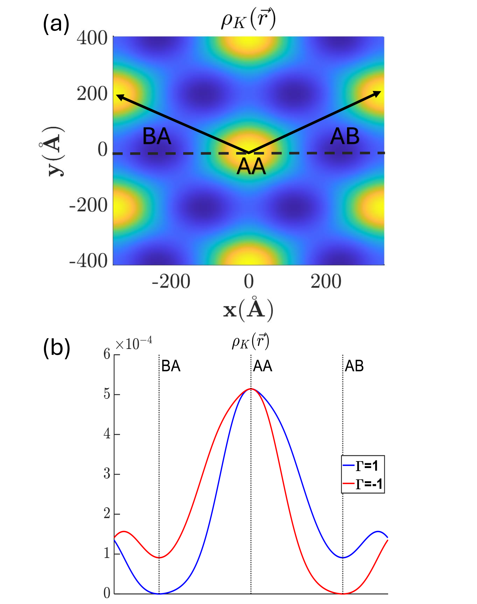
Figure S1: (a) Spatial distribution of the flat-band wave functions at $K$ point in MBZ at the first magic angle for the watermill lattice constant of $a=2.46\text{\AA }$ and twist angle $\theta_{\text{twist}}\cong 0.346^{\circ}$. Black arrows denote the translation vectors of the moiré unit cell. (b) Spatial distribution (up to a normalization factor) of the chirally-symmetric flat-band wave functions at $K$ point in the MBZ with eigenvalues of the chiral symmetry operator $\Gamma=1$ (blue) and $\Gamma=-1$ (red) along the black dashed line in (a) at the first magic angle.

Notably, the chirally symmetric flat-band wave functions at magic angles are zero at the center of the AB/BA stacking regions (FIG. S1(b)). Therefore, such a derivation of magic angles in the CTBWL mirrors the one for the chiral twisted bilayer graphene (CTBG), see Ref. [15] for details. CTBWL thus hosts magic angles that are identical to those in CTBG in accord with the numerical findings presented in the main text for CTBWL and the values reported for CTBG in Ref. [15]. Here, we only show the construction of the flat-band wave functions for the $\psi_{C}^{(\vec{k})}(\vec{r}),\psi_{A_{2}}^{(\vec{k})}(\vec{r})$ components. The other flat-band wave functions can be constructed along similar lines.

II S2. Pseudo-Landau level representation of CTBWL at the first magic angle

At the first magic angle $\alpha_{\text{magic}}^{(1)}$, the wave functions of the isolated flat bands are primarily localized around the AA-stacked region ($\vec{r}=0$) as shown in FIG. S1(a). To analyze the Hamiltonian for these flat bands in the limit $\omega_{1}=\omega_{3}=\omega_{4}=0$, we expand the interlayer tunneling of TBWL in Eq. 5 to order $O(\frac{r}{L_{s}})$ [16]:

$$T\cong\omega_{2}\big{\{}T_{1}(1-i\frac{4\pi y}{3L_{s}})+T_{2}[1+i\frac{2\pi}{3L_{s}}(\sqrt{3}x+y)]+T_{3}[1+i\frac{2\pi}{3L_{s}}(-\sqrt{3}x+y)]\big{\}},$$ (S12)

where $T_{n}=\cos[(n-1)\frac{2\pi}{3}]S_{1}-\sin[(n-1)\frac{2\pi}{3}]S_{2}$. Then, Eq. (S12) can be interpreted as the effective vector potential in the watermill lattice, given by $\vec{A}=-\frac{2\pi\omega_{2}}{L_{s}}(y\hat{x}-\xi x\hat{y})$. The low-energy Hamiltonian in TBWL can, therefore, be expressed as:

$$\begin{split}H=&(\frac{3t}{2}q_{x}\tau_{0}-A_{x}\tau_{2})S_{1}+(\frac{3t}{2}\xi q_{y}\tau_{0}-A_{y}\tau_{2})S_{2}\\ \rightarrow&(\frac{3t}{2}q_{x}\tau_{0}-A_{x}\tau_{3})S_{1}+(\frac{3t}{2}\xi q_{y}\tau_{0}-A_{y}\tau_{3})S_{2},\end{split}$$ (S13)

where we have applied an appropriate basis transformation on the layer degrees of freedom represented by $\mathbf{\tau}$ in the second line and $\vec{S}^{(\theta)}\cong\vec{S}$ for $\theta\ll 1$ is assumed.

In the Landau gauge, $\vec{A}=\frac{4\pi\omega_{2}\xi}{L_{s}}x\hat{y}$ is the effective vector potential and $B=\frac{4\pi\omega_{2}\xi}{L_{s}}$ is the effective field strength for the top layer. By introducing the creation (annihilation) operator for Landau level $a^{\dagger}(a)\equiv\frac{1}{\sqrt{2\hbar eB}}(\pi_{x}\pm i\pi_{y})$ with the canonical momentum $\vec{\pi}\equiv\vec{k}-e\vec{A}$, as well as the cyclotron frequency $\omega_{c}=\frac{3t}{2}\sqrt{\frac{2eB}{\hbar}}$, the Hamiltonian in Eq. (S13) for the top layer can be rewritten as:

$$H=\hbar\omega_{c}\begin{pmatrix}0&\frac{\sqrt{3}}{2}a^{\dagger}&0&0\\ \frac{\sqrt{3}}{2}a&0&a^{\dagger}&0\\ 0&a&0&\frac{\sqrt{3}}{2}a^{\dagger}\\ 0&0&\frac{\sqrt{3}}{2}a&0\end{pmatrix}.$$ (S14)

To obtain the Landau levels, we denote the eigenvalue and eigenstate of the $n^{th}$ Landau level as $E_{n}$ and $\ket{\psi_{n}(k)}$, respectively. We assume that $\ket{\psi_{n}(k)}$can be constructed using the eigenstates of the cyclotron motions, as shown below,

$$\begin{split}\ket{\psi_{n}(k)}=&\frac{e^{ikx}}{\sqrt{2L_{x}l_{B}}}\big{(}u_{n}\begin{pmatrix}1\\ 0\\ 0\\ 0\end{pmatrix}\ket{n}+v_{n}\begin{pmatrix}0\\ 1\\ 0\\ 0\end{pmatrix}\ket{n-1}+\alpha_{n}\begin{pmatrix}0\\ 0\\ 1\\ 0\end{pmatrix}\ket{n-2}+\beta_{n}\begin{pmatrix}0\\ 0\\ 0\\ 1\end{pmatrix}\ket{n-3}\big{)}.\end{split}$$ (S15)

Here, $l_{B}=\sqrt{\frac{3L_{s}\hbar t}{8\pi\omega_{2}}}$ is the magnetic length, $L_{x}$ is the size of the system along the $\hat{x}$ direction, and ($u_{n}$, $v_{n}$, $\alpha_{n}$, $\beta_{n}$) are the complex coefficients of the cyclotron motion eigenstates. The state $\ket{n}$ satisfies $a\ket{n}=\sqrt{n}\ket{n-1}$ and $a^{\dagger}\ket{n}=\sqrt{n+1}\ket{n+1}$. From the eigenvalue equation $H\ket{\psi_{n}(k)}=E_{n}\ket{\psi_{n}(k)}$, we find that $E_{n}$ satisfies the equation:

$$\text{det}\begin{pmatrix}E_{n}&-\hbar\omega_{c}\frac{\sqrt{3}}{2}\sqrt{n}&0&0\\ -\hbar\omega_{c}\frac{\sqrt{3}}{2}\sqrt{n}&E_{n}&-\hbar\omega_{c}\sqrt{n-1}&0\\ 0&-\hbar\omega_{c}\sqrt{n-1}&E_{n}&-\hbar\omega_{c}\frac{\sqrt{3}}{2}\sqrt{n-2}\\ 0&0&-\hbar\omega_{c}\frac{\sqrt{3}}{2}\sqrt{n-2}&E_{n}\end{pmatrix}=0.$$ (S16)

Consequently, the solution to Eq. (S16) can be obtained as follows:

$$E_{0}=0,\quad E_{1}=\pm\frac{\sqrt{3}}{2}\hbar\omega_{c},\quad E_{2}=0\quad\text{or}\quad\pm\frac{\sqrt{10}}{2}\hbar\omega_{c},\text{ and}\quad E_{n}=\pm\frac{\hbar\omega_{c}}{2}\sqrt{5(n-1)\pm 4\sqrt{(n-1)^{2}+\frac{9}{16}}}\quad\forall n\geq 3.$$

Similar results can be obtained for the bottom layer. However, the bottom layer experiences the opposite gauge field compared to the top layer, resulting in a minus sign for its vector potential. The Hamiltonian in Eq. (S14) for the bottom layer then becomes:

$$H=\hbar\omega_{c}\begin{pmatrix}0&\frac{\sqrt{3}}{2}a&0&0\\ \frac{\sqrt{3}}{2}a^{\dagger}&0&a&0\\ 0&a^{\dagger}&0&\frac{\sqrt{3}}{2}a\\ 0&0&\frac{\sqrt{3}}{2}a^{\dagger}&0\end{pmatrix},$$ (S17)

and the ansatz for the eigenstates takes the form:

$$\begin{split}\ket{\psi_{n}(k)}=&\frac{e^{ikx}}{\sqrt{2L_{x}l_{B}}}\big{(}u_{n}\begin{pmatrix}1\\ 0\\ 0\\ 0\end{pmatrix}\ket{n-3}+v_{n}\begin{pmatrix}0\\ 1\\ 0\\ 0\end{pmatrix}\ket{n-2}+\alpha_{n}\begin{pmatrix}0\\ 0\\ 1\\ 0\end{pmatrix}\ket{n-1}+\beta_{n}\begin{pmatrix}0\\ 0\\ 0\\ 1\end{pmatrix}\ket{n}\big{)},\end{split}$$ (S18)

Correspondingly, Eq. (S16) becomes:

$$\text{det}\begin{pmatrix}E_{n}&-\hbar\omega_{c}\frac{\sqrt{3}}{2}\sqrt{n-2}&0&0\\ -\hbar\omega_{c}\frac{\sqrt{3}}{2}\sqrt{n-2}&E_{n}&-\hbar\omega_{c}\sqrt{n-1}&0\\ 0&-\hbar\omega_{c}\sqrt{n-1}&E_{n}&-\hbar\omega_{c}\frac{\sqrt{3}}{2}\sqrt{n}\\ 0&0&-\hbar\omega_{c}\frac{\sqrt{3}}{2}\sqrt{n}&E_{n}\end{pmatrix}=0.$$ (S19)

The Landau levels of the bottom layer are identical to those of the top layer, see Eq. (S16). Consequently, each layer contributes two zero modes, arising from the states with $n=0$ and $n=2$, resulting in the four isolated flat bands observed at the first magic angle, $\alpha_{\text{magic}}^{(1)}$, in CTBWL.

III S3. Wilson-loop winding constrained by the $C_{2z}\mathcal{T}$ symmetry in CTBWL

Following the methods in Ref. [5], we now show that the hybrid Wannier centers exhibit non-trivial windings in CTBWM, and the $C_{2z}\mathcal{T}$ symmetry ensures that the eigenvalues of the Wilson loop of the isolated flat bands are complex conjugates of each other, that is, their Wilson-loop spectrum is symmetric around zero. More specifically, the plane-wave basis describing the low-energy states of CTBWL can be characterized by the valley degree of freedom $\xi=K/K^{\prime}$, layer degree of freedom $\tau=\text{top/bottom}$, orbital degree of freedom on each layer $\sigma=A_{1}^{(\tau)},B^{(\tau)},C^{(\tau)},A_{2}^{(\tau)}$, reciprocal lattice vector $\vec{Q}$, and the momentum $\vec{k}$, denoted as $\ket{\psi_{\xi,\sigma,\vec{Q},\vec{k}}}$. Note that we have assumed the absence of inter-valley scatterings, ensuring a well-defined valley degree of freedom. The unitary representation of the $C_{2z}\mathcal{T}$ symmetry, denoted as $R(C_{2z}\mathcal{T})$, is defined as:

$$\begin{cases}(C_{2z}\mathcal{T})\ket{\psi_{\xi,\sigma=A_{1}^{(\tau)},\vec{Q},\vec{k}}}=R(C_{2z}\mathcal{T})\ket{\psi_{\xi,\sigma=A_{2}^{(\tau)},\vec{Q},\vec{k}}}\\ (C_{2z}\mathcal{T})\ket{\psi_{\xi,\sigma=B^{(\tau)},\vec{Q},\vec{k}}}=R(C_{2z}\mathcal{T})\ket{\psi_{\xi,\sigma=C^{(\tau)},\vec{Q},\vec{k}}}.\end{cases}$$ (S20)

Therefore, $R(C_{2z}\mathcal{T})_{\vec{Q},\sigma;\vec{Q}^{\prime},\sigma^{\prime}}=\delta_{\vec{Q}\vec{Q}^{\prime}}(\tau_{0}\otimes\sigma_{1}\otimes\sigma_{1})_{\sigma\sigma^{\prime}}$. Note that the complete representation of the $C_{2z}\mathcal{T}$ symmetry $R(C_{2z}\mathcal{T})\textit{K}$ is anti-unitary, where K is the anti-linear operator.

In our theory, $T^{2}=1$ since we consider a spinless system. Therefore, we can have a unitary sewing matrix $S(\vec{k})$ for the $C_{2z}\mathcal{T}$ symmetry since there are no Kramers pairs [5],

$$S(\vec{k})=\Psi^{\dagger}(\vec{k})R(C_{2z}\mathcal{T})\Psi^{*}(\vec{k}),$$ (S21)

where $\Psi(\vec{k})=(\ket{\psi_{1}(\vec{k})},\ket{\psi_{2}(\vec{k})},\ket{\psi_{3}(\vec{k})},\ket{\psi_{4}(\vec{k})})$ with $\ket{\psi_{i}(\vec{k})}$ be the $i^{\text{th}}$ isolated flat band expanded on the plane-wave basis. Note that $\Psi(\vec{k})\Psi^{\dagger}(\vec{k})=1$ since $\{\ket{\psi_{i}(\vec{k})}\}$ is a complete basis set in the subspace spanned by the isolated flat bands. Then, according to Eq. (S21),

$$\Psi(\vec{k})S(\vec{k})=R(C_{2z}\mathcal{T})\Psi^{*}(\vec{k}).$$ (S22)

The Wilson loop operator for these isolated flat bands is [72, 73, 74]:

$$W(k_{1})=\lim_{\Delta k\rightarrow 0}\Psi^{\dagger}(k_{1},0)\Psi(k_{1},\Delta k)\Psi^{\dagger}(k_{1},\Delta k)...\Psi^{\dagger}(k_{1},2\pi-\Delta k)\Psi(k_{1},2\pi),$$ (S23)

of which the complex conjugation is [5]:

$$\begin{split}W^{*}(k_{1})&=\lim_{\Delta k\rightarrow 0}\Psi^{T}(k_{1},0)\Psi^{*}(k_{1},\Delta k)\Psi^{T}(k_{1},\Delta k)...\Psi^{T}(k_{1},2\pi-\Delta k)\Psi^{*}(k_{1},2\pi)\\ &=\lim_{\Delta k\rightarrow 0}\Psi^{T}(k_{1},0)R^{-1}(C_{2z}\mathcal{T})R(C_{2z}\mathcal{T})\Psi^{*}(k_{1},\Delta k)\Psi^{T}(k_{1},\Delta k)R^{-1}(C_{2z}\mathcal{T})R(C_{2z}\mathcal{T})...\Psi^{T}(k_{1},2\pi-\Delta k)R^{-1}(C_{2z}\mathcal{T})R(C_{2z}\mathcal{T})\Psi^{*}(k_{1},2\pi)\\ &=\lim_{\Delta k\rightarrow 0}[\Psi(k_{1},0)S(k_{1},0)]^{\dagger}\Psi(k_{1},\Delta k)S(k_{1},\Delta k)[\Psi(k_{1},\Delta k)S(k_{1},\Delta k)]^{\dagger}R(C_{2z}\mathcal{T})...[\Psi(k_{1},2\pi-\Delta k)S(k_{1},2\pi-\Delta k)]^{\dagger}\Psi(k_{1},2\pi)S(k_{1},2\pi)\\ &=S^{\dagger}(k_{1},0)W(k_{1})S(k_{1},2\pi)\\ &=S^{\dagger}(k_{1},0)W(k_{1})S(k_{1},0).\end{split}$$ (S24)

Consequently, the eigenvalues of $W(k_{1})$ exist either as complex-conjugate pairs or as real values because $W(k_{1})$ only differs from its complex conjugate $W^{*}(k_{1})$ by a unitary transformation. Since $W(k_{1})=\mathcal{P}e^{-i\oint dk_{2}^{\prime}A_{2}(k_{1},k_{2}^{\prime})}$, its eigenvalues take the form $e^{i2\pi\theta_{i}}$, where $\mathcal{P}$ is the path ordering operator, and $A_{2}(k_{1},k_{2}^{\prime})=i\Psi^{\dagger}(k_{1},k_{2})\partial\Psi(k_{1},k_{2})/\partial k_{2}$ represents the non-Abelian Berry connection. The set $\{\theta_{i}\mod 1\}$ is recognized as the spectrum of the Wilson loop [75]. Therefore, the Wilson loop exhibits a trivial spectrum if the eigenvalues of $W(k_{1})$ are real, i.e., $\theta_{i}=0,1/2$ for all $k_{1}$. Conversely, for a Wilson loop with a non-trivial spectrum, its eigenvalues must be complex-conjugate pairs, leading to a Wilson loop spectrum $\{\theta_{i}\mod 1\}$ that is symmetric with respect to $0$ [5].

IV S4. Numerical computations for the trace of the quantum weight

Trace of the quantum weight [79] for the bands of interest is:

$$K=2\pi\int\frac{d^{2}k}{(2\pi)^{2}}\,\big{[}g_{xx}(\vec{k})+g_{yy}(\vec{k})\big{]}.$$ (S25)

Here, $g_{\mu\nu}(\vec{k})$ is the quantum metric of the bands of interest, which can be calculated by the projection operator to the bands of interest $P(\vec{k})$ through $g_{\mu\nu}(\vec{k})=\frac{1}{2}\text{Tr}[(\partial_{\mu}P)(\partial_{\nu}P)]$ with $\partial_{\mu}\equiv\partial/\partial{k^{\mu}}$ and $\text{Tr}\big{[}...\big{]}$ indicating the trace over quantum states [5, 6]. The expression of $K$ in Eq. (S25) can be rewritten into a coordinate-invariant form [6]:

$$K^{(\text{inv})}=2\pi\int\frac{d^{2}k}{(2\pi)^{2}}\sqrt{\det(\eta)}\eta^{\nu\mu}g_{\mu\nu}(\vec{k})=2\pi\int\frac{d^{2}k}{(2\pi)^{2}}\sqrt{\det(\eta)}\text{tr}\big{[}\eta^{-1}g(\vec{k})\big{]},$$ (S26)

where $A_{M}$ is the area of the moiré unit cell, and $\text{tr}\big{[}...\big{]}$ indicates the trace over spatial indices. $\eta^{\mu\nu}$ is defined as the inverse of the spatial metric $\eta_{\mu\nu}$ such that $\eta^{\mu\nu}\eta_{\nu\alpha}=\delta^{\mu}_{\alpha}$, where $\eta_{\mu\nu}\equiv\vec{b}_{\mu}\cdot\vec{b}_{\nu}$ with $\vec{b}_{\mu}$ being the reciprocal lattice vector. Note that we have used the convention $\vec{a}_{i}\cdot\vec{b}_{j}=\delta_{ij}$, where $\vec{a}_{i}$ is the translation vector. Consider a transformation $\vec{b}_{\mu}^{\prime}=\sum_{\nu}S_{\mu\nu}\vec{b}_{\nu}$ with $S\in\text{GL}_{2}(\mathbb{R})$. Then, the quantities $\eta_{\mu\nu}$, $\eta^{\mu\nu}$, and $g_{\mu\nu}$ transform as:

$$\eta{{}^{\prime}}= S\eta S^{T}$$

$$\eta{{}^{\prime}}^{-1}= (S^{T})^{-1}\eta^{-1}S^{-1}$$

$$g{{}^{\prime}}(\vec{k})= Sg(\vec{k})S^{T}.$$

Therefore, $\text{tr}\big{[}\eta{{}^{\prime}}^{-1}g{{}^{\prime}}(\vec{k})\big{]}=\text{tr}\big{[}\eta^{-1}g(\vec{k})\big{]}$, and the integarl in Eq. (S26) is invariant under transformation of $\{\vec{b}_{\mu}\}$ with the corresponding Jacobian $\sqrt{\det(\eta)}$ for the integral measure. $K$ in Eq. (S25) can thus be recovered by $K^{\text{(inv)}}$ in Eq. (S26) by transforming $\{\vec{b}_{\mu}\}$ into a frame in which $\vec{b}_{1}\cdot\vec{b}_{2}=0$ if $\|\vec{b}_{1}\|=\|\vec{b}_{2}\|$. For example, if we have $\vec{b}_{1}=\frac{2\pi}{a}(\frac{1}{2}\hat{x}+\frac{\sqrt{3}}{2}\hat{y})$ and $\vec{b}_{2}=\frac{2\pi}{a}(-\frac{1}{2}\hat{x}+\frac{\sqrt{3}}{2}\hat{y})$ so $\|\vec{b}_{1}\|=\|\vec{b}_{2}\|$, we can transform them into a frame where $\vec{b}_{1}^{\prime}=\vec{b}_{1}-\vec{b}_{2}=\frac{2\pi}{a}\hat{x}$ and $\vec{b}_{2}^{\prime}=\frac{1}{\sqrt{3}}(\vec{b}_{1}+\vec{b}_{2})=\frac{2\pi}{a}\hat{y}$. At that time, $S=\begin{pmatrix}1&-1\\ \frac{1}{\sqrt{3}}&\frac{1}{\sqrt{3}}\end{pmatrix}$, $\vec{b}_{1}^{\prime}\cdot\vec{b}_{2}^{\prime}=0$, and $\|\vec{b}_{1}^{\prime}\|=\|\vec{b}_{2}^{\prime}\|$ so $K=K^{(\text{inv})}$.

We further expand Eq. (S26) into a more convenient form for numerical computation [6]:

$$K^{(\text{inv})}=2\pi\int\frac{dk^{1}dk^{2}}{(2\pi)^{2}A_{M}}\eta^{\nu\mu}\frac{1}{2}\text{Tr}[(\partial_{\mu}P)(\partial_{\nu}P)],$$ (S27)

where $A_{M}$ is the area of the moiré unit cell and $\text{Tr}[...]$ indicates trace over the quantum states. We numerically evaluate $\frac{1}{2}\text{Tr}\big{[}(\partial_{\mu}P)(\partial_{\nu}P)\big{]}$ using a finite difference method via:

$$\begin{split}\frac{1}{2}\text{Tr}\big{\{}[\partial_{\mu}P(\vec{k})][\partial_{\nu}P(\vec{k})]\big{\}}&\rightarrow\frac{1}{2\epsilon^{2}}\text{Tr}\big{\{}[P(\vec{k}+\epsilon\vec{b}_{\mu})-P(\vec{k})][P(\vec{k}+\epsilon\vec{b}_{\nu})-P(\vec{k})]\big{\}}\\ &=\frac{1}{2\epsilon^{2}}\text{Tr}\big{[}P(\vec{k}+\epsilon\vec{b}_{\mu})P(\vec{k}+\epsilon\vec{b}_{\nu})+P(\vec{k})^{2}-P(\vec{k}+\epsilon\vec{b}_{\mu})P(\vec{k})-P(\vec{k}+\epsilon\vec{b}_{\nu})P(\vec{k})\big{]}\\ &=\frac{1}{2\epsilon^{2}}\bigg{\{}\text{Tr}\big{[}P(\vec{k}+\epsilon\vec{b}_{\mu})P(\vec{k}+\epsilon\vec{b}_{\nu})\big{]}+N-\text{Tr}\big{[}P(\vec{k}+\epsilon\vec{b}_{\mu})P(\vec{k})\big{]}-\text{Tr}\big{[}P(\vec{k}+\epsilon\vec{b}_{\nu})P(\vec{k})\big{]}\bigg{\}}\end{split}$$ (S28)

where $N\equiv\text{Tr}\big{[}P(\vec{k})\big{]}$ is the number of bands of interest. Then, by using a $l\times l$ grid on the Brillouin zone for numerical integration, Eq. (S27) can be rewritten as:

$$\begin{split}K^{(\text{inv})}=\frac{1}{2\pi}\sum_{\vec{k}}\frac{1}{l^{2}}\frac{\eta^{\mu\nu}}{A_{M}}\frac{1}{2\epsilon^{2}}\bigg{\{}\text{Tr}\big{[}P(\vec{k}+\epsilon\vec{b}_{\mu})P(\vec{k}+\epsilon\vec{b}_{\nu})\big{]}+N-\text{Tr}\big{[}P(\vec{k}+\epsilon\vec{b}_{\mu})P(\vec{k})\big{]}-\text{Tr}\big{[}P(\vec{k}+\epsilon\vec{b}_{\nu})P(\vec{k})\big{]}\bigg{\}},\end{split}$$ (S29)

which can be computed efficiently by choosing $\epsilon=\frac{1}{l}$. More specifically, we consider the quantity:

$$F_{(1)}(k^{1},k^{2})\equiv N-\text{Tr}\big{[}P(k^{1}+\epsilon,k^{2})P(k^{1},k^{2})\big{]}.$$ (S30)

Note that we have denoted $P(\vec{k}=k^{\mu}\vec{b}_{\mu})$ as $P(k^{1},k^{2})$. On a $l\times l$ grid of the Brillouin zone with $\epsilon=\frac{1}{l}$, Eq. (S30) becomes:

$$F_{(1)}(n,m)=N-\text{Tr}\big{[}P(\frac{n+1}{l},\frac{m}{l})P(\frac{n}{l},\frac{m}{l})\big{]},$$ (S31)

in which $n,m=0,...,l-1$. Similarly, we can define:

$$F_{(2)}(k^{1},k^{2})\equiv N-\text{Tr}\big{[}P(k^{1},k^{2}+\epsilon)P(k^{1},k^{2})\big{]},$$ (S32)

and its corresponding discrete representation:

$$F_{(2)}(n,m)\equiv N-\text{Tr}\big{[}P(\frac{n}{l},\frac{m+1}{l})P(\frac{n}{l},\frac{m}{l})\big{]}.$$ (S33)

Consider another quantity:

$$\tilde{F}_{(\mu\nu)}(\vec{k})\equiv\text{Tr}\big{[}P(\vec{k}+\epsilon\vec{b}_{\mu})P(\vec{k}+\epsilon\vec{b}_{\nu})\big{]}-N.$$ (S34)

Then, on a $l\times l$ grid of the Brillouin zone with $\epsilon=\frac{1}{l}$,

$$\tilde{F}_{(12)}(n,m)=\tilde{F}_{(21)}(n,m)=\text{Tr}\big{[}P(\frac{n+1}{l},\frac{m}{l})P(\frac{n}{l},\frac{m+1}{l})\big{]}-N,$$ (S35)

and:

$$\tilde{F}_{(11)}(n,m)=\text{Tr}\big{[}P(\frac{n+1}{l},\frac{m}{l})P(\frac{n+1}{l},\frac{m}{l})\big{]}-N=0.$$ (S36)

Similarly, $\tilde{F}_{(22)}(n,m)=0$. Note that $P(1,\frac{m}{l})=V(\vec{b}_{1})P(0,\frac{m}{l})V^{\dagger}(\vec{b}_{1})$ with $m\neq l$ and $P(\frac{n}{l},1)=V(\vec{b}_{2})P(\frac{n}{l},0)V^{\dagger}(\vec{b}_{2})$ with $n\neq l$, where $V(\vec{b}_{\mu})$ is the embedding matrix in the direction of the reciprocal lattice vector $\vec{b}_{\mu}$ such that $(V(\vec{b}_{\mu}))_{ij}=\delta_{ij}e^{-i2\pi\vec{b}_{\mu}\cdot r_{i}}$ [6]. Therefore, combining the results from Eq. (S30) to Eq. (S36), Eq. (S29) can be computed efficiently through:

$$K^{(\text{inv})}=\frac{1}{2\pi A_{M}}\sum_{n,m=0}^{l-1}\bigg{[}\eta^{12}\tilde{F}_{(12)}(n,m)+\sum_{\mu=1}^{2}(\eta^{\mu\mu}+\eta^{12})F_{(\mu)}(n,m)\bigg{]}.$$ (S37)

V S5. Geometric contribution to the superfluid weight in CTBWL

We consider a mean-field theory described by a Bogoliubov-de-Gennes Hamiltonian with a pairing potential [5]

$$\Delta(\vec{k})=[\Delta(T)P(\vec{k})]U.$$ (S38)

Here, $\Delta(T)\in\mathbb{R}$, $P(\vec{k})$ is the projection operator to the flat bands, and $U$ is the unitary part of the time-reversal operator. We use the fact that the flat bands are exactly flat with a substantial band gap $E_{\text{gap}}$ between them and other high-energy bands at magic angles, such that there is no pairing between the flat bands and other high-energy bands. Also, $E_{\text{gap}}\gg\Delta(T)$ is assumed since the pairing potentials are weak. Then, the geometric contribution to their superfluid weight dominates [7, 8] and the resulting isotropic superfluid weight is give by:

$$D_{s}(T)=\frac{\delta^{\mu\nu}D_{\mu\nu}(T)}{2}=\frac{e^{2}\Delta(T)^{2}}{4\pi\hbar^{2}\sqrt{(E_{0}-\mu)^{2}+\Delta(T)^{2}}}\tanh({\frac{\beta\sqrt{(E_{0}-\mu)^{2}+\Delta(T)^{2}}}{2}})K$$ (S39)

for the isolated flat bands in CTBWL at a magic angle, where the chemical potential, $\mu$, is related through the filling factor, $\nu$, by:

$$\nu=\frac{1}{2}(1-\frac{E_{0}-\mu}{\sqrt{(E_{0}-\mu)^{2}+\Delta(T)^{2}}})+\frac{1}{e^{\beta\sqrt{(E_{0}-\mu)^{2}+\Delta(T)^{2}}}+1},$$ (S40)

along the lines of Ref. 5. Here, $E_{0}$ is the flat band energy and $\beta\equiv(k_{B}T)^{-1}$. Further, we assume the celebrated scaling form of the order parameter $\Delta(T)\cong 3k_{B}T_{\text{MF}}\sqrt{1-\frac{T}{T_{\text{MF}}}}$ around the mean-field transition temperature, $T_{\text{MF}}$, in the BCS theory [76]. Berezinskii-Kosterlitz-Thouless (BKT) transition temperature, $T_{\text{BKT}}$, is then given by[80],

$$k_{B}T_{\text{BKT}}=\frac{\pi\hbar^{2}}{8e^{2}}D_{s}(T_{\text{BKT}}).$$ (S41)

The BKT transition temperature can be obtained by self-consistently solving Eq. (S41) with Eq. (S39), where the chemical potential is obtained by solving Eq. (S40) for a given filling factor, $\nu$. The trace of quantum weight originating from every spin and valley was included in obtaining the numerical values listed in the main text.

VI S6. Modified hopping strength in watermill lattice and CTBWL

If the hopping strength between orbitals $B$ and $C$ has a different ratio $\gamma\in\mathbb{R}$ than the strength of hopping between other orbitals, Eq. (2) can be written as:

$$H_{0}^{\prime}(\vec{k})=t\begin{pmatrix}0&\frac{\sqrt{3}}{2}k_{-}&0&0\\ \frac{\sqrt{3}}{2}k_{+}&0&\gamma k_{-}&0\\ 0&\gamma k_{+}&0&\frac{\sqrt{3}}{2}k_{-}\\ 0&0&\frac{\sqrt{3}}{2}k_{+}&0\end{pmatrix}.$$ (S42)

Here, without loss of generality, we consider the low-energy states at $K$-valley by taking $\xi=+$. Then, the eigenenergies of Eq. (S42) are:

$$E=\zeta t\frac{\|\vec{k}\|}{2}\sqrt{(3+2\gamma^{2})+2\lambda|\gamma|\sqrt{3+\gamma^{2}}}$$ (S43)

with the corresponding eigenstates labeled as $\ket{\zeta,\lambda}$, where $\zeta,\lambda=\pm 1$. Equation (S43) reduces to the dispersion of Eq. (2) when $|\gamma|=1$. Since $|3+2\gamma^{2}|>|2\gamma\sqrt{3+\gamma^{2}}|$, the dispersion only becomes degenerate at $\|\vec{k}\|=0$ with a four-fold degeneracy. Note that Eq. (S42) still preserves the $C_{2z}\mathcal{T}$ symmetry and the chiral symmetry $\Gamma$ for arbitrary value of $\gamma$. The pseudospin texture for each band is:

$$\bra{\zeta,\lambda}\vec{S}(\vec{k})\ket{\zeta,\lambda}=\zeta\frac{2\vec{k}}{3\|\vec{k}\|}\sqrt{3+2\gamma^{2}+2\lambda|\gamma|\sqrt{3+\gamma^{2}}}\bigg{[}3+\gamma+\lambda\,\text{sign}(\gamma)\sqrt{3+\gamma^{2}}\bigg{]}.$$ (S44)

Since the pseudospin texture $\vec{S}(\vec{k})\propto\zeta\frac{\vec{k}}{\|\vec{k}\|}$, each band has a non-trivial winding pattern of the pseudospin texture with the winding number $w=\zeta$. Similarly, the bands of the low-energy states at the $K^{\prime}$-valley would exhibit a pseudospin texture $\vec{S}(\vec{k})\propto-\zeta\frac{\vec{k}}{\|\vec{k}\|}$ with the winding number $w=-\zeta$. However, the magic angles in the corresponding CTBWL persist at the same values, and Eq. (S1) becomes:

$$H=\begin{pmatrix}0&0&\frac{\sqrt{3}}{2}D(\vec{r})&0\\ 0&0&\tilde{D}^{*}(-\vec{r})&\frac{\sqrt{3}}{2}D(\vec{r})\\ \frac{\sqrt{3}}{2}D^{*}(-\vec{r})&\tilde{D}(\vec{r})&0&0\\ 0&\frac{\sqrt{3}}{2}D^{*}(-\vec{r})&0&0\end{pmatrix},$$ (S45)

where

$$\tilde{D}(\vec{r})=\begin{pmatrix}-i\gamma\bar{\partial}&\alpha t(\vec{r})\\ \alpha t(-\vec{r})&-i\gamma\bar{\partial}\end{pmatrix}.$$ (S46)

The flat-band wave function in Eq. (S7) thus remains the same but the one in Eqs. (S6) and (S8) would be modified:

$$\delta\psi_{C}^{(\vec{k})}(\vec{r})=-\frac{2}{\sqrt{3}}D^{-1}(\vec{r})\tilde{D}^{*}(-\vec{r})h^{(\vec{k})}(z)\phi_{C}^{(K)}(\vec{r}).$$ (S47)

Nonetheless, based on the results of the preceding SM section, the method for finding magic angles (Eq. (S7)) stays unchanged, and the magic angles remain consistent even if the interlayer tunneling strength between orbitals $B$ and $C$ is altered to be $\delta\cdot\alpha$ for a certain constant value $\delta$. Generally speaking, as long as the structure of $D(\vec{r})$ in Eq. (S45) remains intact, the magic angles retain the values they have in the CTBWL with unmodified hopping strengths. In any event, the magic angles can still be calculated using the techniques already discussed above. An illustrative example is presented in FIG. S4, where $\omega_{2}^{\prime}=\omega_{2}=\alpha vk_{\theta}$ so that Eq. (S45) becomes:

$$H=\begin{pmatrix}0&0&\frac{\sqrt{3}}{2}\Delta(\vec{r})&0\\ 0&0&D^{*}(-\vec{r})&\frac{\sqrt{3}}{2}\Delta(\vec{r})\\ \frac{\sqrt{3}}{2}\Delta^{*}(-\vec{r})&D(\vec{r})&0&0\\ 0&\frac{\sqrt{3}}{2}\Delta^{*}(-\vec{r})&0&0\end{pmatrix}.$$ (S48)

Here:

$$\Delta(\vec{r})=\begin{pmatrix}-i\bar{\partial}&\tilde{\alpha}t(\vec{r})\\ \tilde{\alpha}t(-\vec{r})&-i\bar{\partial}\end{pmatrix},$$ (S49)

where $\tilde{\alpha}=\frac{2}{\sqrt{3}}\alpha$. As a result, the magic angles are roughly $\frac{\sqrt{3}}{2}$ times their original values, which is consistent with the numerical results shown in FIG. S4.

Notably, the pseudo-Landau level representation for the corresponding CTBWL at magic angles continues to produce four zero modes. As previously illustrated, these distinct flat bands can be interpreted as zero modes of the CTBWL. By modifying the hopping ratio, the method described in Eq. (S16) can be applied to calculate the pseudo-Landau levels’ energy, yielding the following values for the two layer:

$$E_{0}=0,\quad E_{1}=\pm\frac{\sqrt{3}}{2}\hbar\omega_{c},\quad E_{2}=0\quad\text{or }\pm\frac{\sqrt{6+4\gamma^{2}}}{2}\hbar\omega_{c},$$

$$\text{and }E_{n}=\pm\frac{\hbar\omega_{c}}{2}\sqrt{(3+2\gamma^{2})(n-1)\pm\sqrt{4\gamma^{2}(3+\gamma^{2})(n-1)^{2}+9}}\quad\forall n\geq 3,$$

demonstrating that the zero modes still originate from the $n=0$ and $n=2$ pseudo-Landau levels.

VII S7. Effect of onsite potential difference in CTBWL

The onsite potentials break the sublattice symmetry in the watermill lattice and CTBWL, opening the gap at the $K,K^{\prime}$ valley. We now consider the effects of onsite potential difference between the sites $A$ and $B/C$. In the watermill lattice, the Berry curvature accumulates around the valley after gap-opening due to differences in onsite potentials. The band structure still hosts a two-fold degeneracy in both the valence and conduction bands. The onsite potential induces a Dirac cone and a quadratic touching in the valence and conduction bands, respectively, with zero total Berry curvature around the valley (FIGS. S2(a) and  S2(b)).

In the pseudo-Landau level representation for the first magic angle in CTBWL subjected to different onsite potentials on various orbitals, Eq. (S16) (i.e., pseudo-Landau levels at the top layer) becomes:

$$\text{det}\begin{pmatrix}E_{n}^{(\text{top})}-\Delta E_{A_{1}}&-\hbar\omega_{c}\frac{\sqrt{3}}{2}\sqrt{n}&0&0\\ -\hbar\omega_{c}\frac{\sqrt{3}}{2}\sqrt{n}&E_{n}^{(\text{top})}-\Delta E_{B}&-\hbar\omega_{c}\sqrt{n-1}&0\\ 0&-\hbar\omega_{c}\sqrt{n-1}&E_{n}^{(\text{top})}-\Delta E_{C}&-\hbar\omega_{c}\frac{\sqrt{3}}{2}\sqrt{n-2}\\ 0&0&-\hbar\omega_{c}\frac{\sqrt{3}}{2}\sqrt{n-2}&E_{n}^{(\text{top})}-\Delta E_{A_{2}}\end{pmatrix}=0.$$ (S50)

The solution of Eq. (S17) is straightforwardly shown to be: $E_{0}^{(\text{top})}=\Delta E_{A_{1}}$ and $E_{n}^{(\text{top})}=E_{n}^{(\text{top})}(\hbar\omega_{c},\Delta E_{i})\neq\Delta E_{i}\text{ or }0$ for $n\neq 0$. Similarly, Eq. (S19) (i.e., pseudo-Landau levels at the bottom layer) becomes:

$$\text{det}\begin{pmatrix}E_{n}^{(\text{bot})}-\Delta E_{A_{1}}&-\hbar\omega_{c}\frac{\sqrt{3}}{2}\sqrt{n-2}&0&0\\ -\hbar\omega_{c}\frac{\sqrt{3}}{2}\sqrt{n-2}&E_{n}^{(\text{bot})}-\Delta E_{B}&-\hbar\omega_{c}\sqrt{n-1}&0\\ 0&-\hbar\omega_{c}\sqrt{n-1}&E_{n}^{(\text{bot})}-\Delta E_{C}&-\hbar\omega_{c}\frac{\sqrt{3}}{2}\sqrt{n}\\ 0&0&-\hbar\omega_{c}\frac{\sqrt{3}}{2}\sqrt{n}&E_{n}^{(\text{bot})}-\Delta E_{A_{2}}\end{pmatrix}=0,$$ (S51)

which has the solution for $E_{0}^{(\text{bot})}=\Delta E_{A_{2}}$ and $E_{n}^{(\text{bot})}=E_{n}^{(\text{bot})}(\hbar\omega_{c},\Delta E_{i})\neq\Delta E_{i}\text{ or }0$ for $n\neq 0$. In our case, the CTBWL subject to an onsite potential difference $\Delta E$ between the sites A and B/C such that $\Delta E_{A_{1}}=\Delta E_{A_{2}}=\Delta E$ and $\Delta E_{B}=\Delta E_{C}=-\Delta E$, and Eqs. (S50) and (S51) has the same solution. When $\Delta E\ll 1$, the value of $E_{2}^{(\text{top/bot})}$ that is closest to 0 can be approximated by $E_{2}^{(\text{top/bot})}\cong-\frac{\Delta E}{5}$. Therefore, together with the two flat bands from the solution $E_{0}^{(\text{top/bot})}=\Delta E$ in both layers, CTBWL still hosts four isolated flat bands near the Fermi level subjected to a weak onsite potential difference between A and B/C sites. The isolated flat bands thus split into two groups separated by a small band gap with two entangled flat bands in each group, which is confirmed by our numerical results, see FIG. S2(c). The flat bands in the group with higher energy are exactly flat, while the flat bands in the group with lower energy have a very small but finite bandwidth at the original magic angles (FIG. S3(a)). The flat bands in each group still host non-trivial windings of their hybrid Wannier centers (FIGS. S3(b) and (c)). Since the considered onsite potential difference preserves $C_{2z}\mathcal{T}$ symmetry, such a non-trivial winding of hybrid Wannier centers provides a lower bound for the trace of quantum metric for the two isolated flat bands in each group [5].

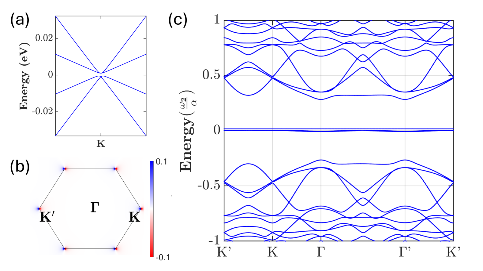
Figure S2: (a) Band structure of the watermill lattice around $K$ valley with onsite energy difference $\Delta E=1$ meV between site $A$ and $B/C$ sites, and (b) the corresponding valence band Berry curvature distribution in the monolayer Brillouin zone. (c) Band structure of the corresponding CTBWL at the first magic angle.

Figure S3: (a) The smallest band gap between the four isolated flat bands near the Fermi level with other high-energy bands ($\Delta_{\text{gap}}$; black). Gap between the two groups of flat bands ($\Delta_{\text{flat}}$; red), and the bandwidth of the flat bands in each group ($W_{\text{top}}$ and $W_{\text{bot}}$; blue and green, respectively) as a function of $\alpha$ in CTBWL subjected to onsite potential difference $\Delta E=1$ meV between the sites A and B/C. The indices top and bot indicate the top and bottom pairs of flat bands. Vertical dashed lines indicate the $i^{\text{th}}$ magic angle, $\alpha_{\text{magic}}^{(i)}$. (b) Wilson-loop spectrum of the top two flat bands in the gapped regions (gray) labeled by the $\alpha_{\text{magic}}^{(i)}$ within. (c) Wilson-loop spectrum of the bottom two flat bands in the gapped regions (gray) labeled by the $\alpha_{\text{magic}}^{(i)}$ within.

References

- Andrei et al. [2021] E. Y. Andrei, D. K. Efetov, P. Jarillo-Herrero, A. H. MacDonald, K. F. Mak, T. Senthil, E. Tutuc, A. Yazdani, and A. F. Young, The marvels of moiré materials, Nature Reviews Materials 6, 201 (2021).
- Zhang et al. [2017] C. Zhang, C.-P. Chuu, X. Ren, M.-Y. Li, L.-J. Li, C. Jin, M.-Y. Chou, and C.-K. Shih, Interlayer couplings, moiré patterns, and 2d electronic superlattices in mos2/wse2 hetero-bilayers, Science Advances 3, e1601459 (2017).
- Wintterlin and Bocquet [2009] J. Wintterlin and M.-L. Bocquet, Graphene on metal surfaces, Surface Science 603, 1841 (2009), special Issue of Surface Science dedicated to Prof. Dr. Dr. h.c. mult. Gerhard Ertl, Nobel-Laureate in Chemistry 2007.
- Andrei and MacDonald [2020] E. Y. Andrei and A. H. MacDonald, Graphene bilayers with a twist, Nature Materials 19, 1265 (2020).
- Xie et al. [2020] F. Xie, Z. Song, B. Lian, and B. A. Bernevig, Topology-bounded superfluid weight in twisted bilayer graphene, Phys. Rev. Lett. 124, 167002 (2020).
- Herzog-Arbeitman et al. [2022] J. Herzog-Arbeitman, V. Peri, F. Schindler, S. D. Huber, and B. A. Bernevig, Superfluid weight bounds from symmetry and quantum geometry in flat bands, Phys. Rev. Lett. 128, 087002 (2022).
- Liang et al. [2017] L. Liang, T. I. Vanhala, S. Peotta, T. Siro, A. Harju, and P. Törmä, Band geometry, berry curvature, and superfluid weight, Phys. Rev. B 95, 024515 (2017).
- Peotta and Törmä [2015] S. Peotta and P. Törmä, Superfluidity in topologically nontrivial flat bands, Nature Communications 6, 8944 (2015).
- Julku et al. [2016] A. Julku, S. Peotta, T. I. Vanhala, D.-H. Kim, and P. Törmä, Geometric origin of superfluidity in the lieb-lattice flat band, Phys. Rev. Lett. 117, 045303 (2016).
- Du et al. [2023] L. Du, M. R. Molas, Z. Huang, G. Zhang, F. Wang, and Z. Sun, Moiré photonics and optoelectronics, Science 379, eadg0014 (2023).
- Topp et al. [2021] G. E. Topp, C. J. Eckhardt, D. M. Kennes, M. A. Sentef, and P. Törmä, Light-matter coupling and quantum geometry in moiré materials, Phys. Rev. B 104, 064306 (2021).
- Tai and Claassen [2023] W. T. Tai and M. Claassen, Quantum-geometric light-matter coupling in correlated quantum materials (2023), arXiv:2303.01597 [cond-mat.str-el] .
- Chaudhary et al. [2022] S. Chaudhary, C. Lewandowski, and G. Refael, Shift-current response as a probe of quantum geometry and electron-electron interactions in twisted bilayer graphene, Phys. Rev. Res. 4, 013164 (2022).
- Bistritzer and MacDonald [2011] R. Bistritzer and A. H. MacDonald, Moiré bands in twisted double-layer graphene, Proceedings of the National Academy of Sciences 108, 12233 (2011).
- Tarnopolsky et al. [2019] G. Tarnopolsky, A. J. Kruchkov, and A. Vishwanath, Origin of magic angles in twisted bilayer graphene, Phys. Rev. Lett. 122, 106405 (2019).
- Liu et al. [2019] J. Liu, J. Liu, and X. Dai, Pseudo landau level representation of twisted bilayer graphene: Band topology and implications on the correlated insulating phase, Phys. Rev. B 99, 155415 (2019).
- Song et al. [2019] Z. Song, Z. Wang, W. Shi, G. Li, C. Fang, and B. A. Bernevig, All magic angles in twisted bilayer graphene are topological, Phys. Rev. Lett. 123, 036401 (2019).
- Cao et al. [2018a] Y. Cao, V. Fatemi, S. Fang, K. Watanabe, T. Taniguchi, E. Kaxiras, and P. Jarillo-Herrero, Unconventional superconductivity in magic-angle graphene superlattices, Nature 556, 43 (2018a).
- Cao et al. [2018b] Y. Cao, V. Fatemi, S. Fang, K. Watanabe, T. Taniguchi, E. Kaxiras, and P. Jarillo-Herrero, Unconventional superconductivity in magic-angle graphene superlattices, Nature 556, 43 (2018b).
- Oh et al. [2021] M. Oh, K. P. Nuckolls, D. Wong, R. L. Lee, X. Liu, K. Watanabe, T. Taniguchi, and A. Yazdani, Evidence for unconventional superconductivity in twisted bilayer graphene, Nature 600, 240 (2021).
- Yankowitz et al. [2019] M. Yankowitz, S. Chen, H. Polshyn, Y. Zhang, K. Watanabe, T. Taniguchi, D. Graf, A. F. Young, and C. R. Dean, Tuning superconductivity in twisted bilayer graphene, Science 363, 1059 (2019).
- Isobe et al. [2018] H. Isobe, N. F. Q. Yuan, and L. Fu, Unconventional superconductivity and density waves in twisted bilayer graphene, Phys. Rev. X 8, 041041 (2018).
- Po et al. [2018] H. C. Po, L. Zou, A. Vishwanath, and T. Senthil, Origin of mott insulating behavior and superconductivity in twisted bilayer graphene, Phys. Rev. X 8, 031089 (2018).
- Kwan et al. [2021] Y. H. Kwan, G. Wagner, N. Chakraborty, S. H. Simon, and S. A. Parameswaran, Domain wall competition in the chern insulating regime of twisted bilayer graphene, Phys. Rev. B 104, 115404 (2021).
- Wu et al. [2019] F. Wu, T. Lovorn, E. Tutuc, I. Martin, and A. H. MacDonald, Topological insulators in twisted transition metal dichalcogenide homobilayers, Phys. Rev. Lett. 122, 086402 (2019).
- Angeli and MacDonald [2021] M. Angeli and A. H. MacDonald, valley transition metal dichalcogenide moiré bands, Proceedings of the National Academy of Sciences 118, e2021826118 (2021).
- Devakul et al. [2021] T. Devakul, V. Crépel, Y. Zhang, and L. Fu, Magic in twisted transition metal dichalcogenide bilayers, Nature Communications 12, 6730 (2021).
- Wang et al. [2020] L. Wang, E.-M. Shih, A. Ghiotto, L. Xian, D. A. Rhodes, C. Tan, M. Claassen, D. M. Kennes, Y. Bai, B. Kim, K. Watanabe, T. Taniguchi, X. Zhu, J. Hone, A. Rubio, A. N. Pasupathy, and C. R. Dean, Correlated electronic phases in twisted bilayer transition metal dichalcogenides, Nature Materials 19, 861 (2020).
- Guo et al. [2025] Y. Guo, J. Pack, J. Swann, L. Holtzman, M. Cothrine, K. Watanabe, T. Taniguchi, D. G. Mandrus, K. Barmak, J. Hone, A. J. Millis, A. Pasupathy, and C. R. Dean, Superconductivity in 5.0° twisted bilayer wse2, Nature 637, 839 (2025).
- Cai et al. [2023] J. Cai, E. Anderson, C. Wang, X. Zhang, X. Liu, W. Holtzmann, Y. Zhang, F. Fan, T. Taniguchi, K. Watanabe, Y. Ran, T. Cao, L. Fu, D. Xiao, W. Yao, and X. Xu, Signatures of fractional quantum anomalous hall states in twisted MoTe2, Nature 622, 63 (2023).
- Park et al. [2023] H. Park, J. Cai, E. Anderson, Y. Zhang, J. Zhu, X. Liu, C. Wang, W. Holtzmann, C. Hu, Z. Liu, T. Taniguchi, K. Watanabe, J.-H. Chu, T. Cao, L. Fu, W. Yao, C.-Z. Chang, D. Cobden, D. Xiao, and X. Xu, Observation of fractionally quantized anomalous hall effect, Nature 622, 74 (2023).
- Reddy et al. [2023] A. P. Reddy, F. Alsallom, Y. Zhang, T. Devakul, and L. Fu, Fractional quantum anomalous hall states in twisted bilayer MoTe2 and WSe2, Phys. Rev. B 108, 085117 (2023).
- Xu et al. [2023] F. Xu, Z. Sun, T. Jia, C. Liu, C. Xu, C. Li, Y. Gu, K. Watanabe, T. Taniguchi, B. Tong, J. Jia, Z. Shi, S. Jiang, Y. Zhang, X. Liu, and T. Li, Observation of integer and fractional quantum anomalous hall effects in twisted bilayer MoTe2, Phys. Rev. X 13, 031037 (2023).
- Jin et al. [2019] C. Jin, E. C. Regan, A. Yan, M. Iqbal Bakti Utama, D. Wang, S. Zhao, Y. Qin, S. Yang, Z. Zheng, S. Shi, K. Watanabe, T. Taniguchi, S. Tongay, A. Zettl, and F. Wang, Observation of moiré excitons in WSe2/WS2 heterostructure superlattices, Nature 567, 76 (2019).
- Yuan et al. [2020] L. Yuan, B. Zheng, J. Kunstmann, T. Brumme, A. B. Kuc, C. Ma, S. Deng, D. Blach, A. Pan, and L. Huang, Twist-angle-dependent interlayer exciton diffusion in WS2–WSe2 heterobilayers, Nature Materials 19, 617 (2020).
- Shimazaki et al. [2020] Y. Shimazaki, I. Schwartz, K. Watanabe, T. Taniguchi, M. Kroner, and A. Imamoğlu, Strongly correlated electrons and hybrid excitons in a moiré heterostructure, Nature 580, 472 (2020).
- Jiang et al. [2021a] Y. Jiang, S. Chen, W. Zheng, B. Zheng, and A. Pan, Interlayer exciton formation, relaxation, and transport in tmd van der waals heterostructures, Light: Science & Applications 10, 72 (2021a).
- Wilson et al. [2021] N. P. Wilson, W. Yao, J. Shan, and X. Xu, Excitons and emergent quantum phenomena in stacked 2d semiconductors, Nature 599, 383 (2021).
- Balents et al. [2020] L. Balents, C. R. Dean, D. K. Efetov, and A. F. Young, Superconductivity and strong correlations in moiré flat bands, Nature Physics 16, 725 (2020).
- Tran et al. [2019] K. Tran, G. Moody, F. Wu, X. Lu, J. Choi, K. Kim, A. Rai, D. A. Sanchez, J. Quan, A. Singh, J. Embley, A. Zepeda, M. Campbell, T. Autry, T. Taniguchi, K. Watanabe, N. Lu, S. K. Banerjee, K. L. Silverman, S. Kim, E. Tutuc, L. Yang, A. H. MacDonald, and X. Li, Evidence for moiré excitons in van der waals heterostructures, Nature 567, 71 (2019).
- Morales-Durán et al. [2022] N. Morales-Durán, N. C. Hu, P. Potasz, and A. H. MacDonald, Nonlocal interactions in moiré hubbard systems, Phys. Rev. Lett. 128, 217202 (2022).
- Venderbos and Fernandes [2018] J. W. F. Venderbos and R. M. Fernandes, Correlations and electronic order in a two-orbital honeycomb lattice model for twisted bilayer graphene, Phys. Rev. B 98, 245103 (2018).
- Seo et al. [2019] K. Seo, V. N. Kotov, and B. Uchoa, Ferromagnetic mott state in twisted graphene bilayers at the magic angle, Phys. Rev. Lett. 122, 246402 (2019).
- Pan et al. [2020a] H. Pan, F. Wu, and S. Das Sarma, Quantum phase diagram of a moiré-hubbard model, Phys. Rev. B 102, 201104 (2020a).
- Pan et al. [2020b] H. Pan, F. Wu, and S. Das Sarma, Band topology, hubbard model, heisenberg model, and dzyaloshinskii-moriya interaction in twisted bilayer , Phys. Rev. Res. 2, 033087 (2020b).
- Wang et al. [2024] H. Wang, Y. Fan, and H. Zhang, Electrically tunable high-chern-number quasiflat bands in twisted antiferromagnetic topological insulators, Phys. Rev. B 110, 085135 (2024).
- Akif Keskiner et al. [2024] M. Akif Keskiner, P. Ghaemi, M. Ö. Oktel, and O. Erten, Theory of moiré magnetism and multidomain spin textures in twisted mott insulator–semimetal heterobilayers, Nano Letters 24, 8575 (2024).
- Wang and Zou [2022] E. Wang and X. Zou, Moiré bands in twisted trilayer black phosphorene: effects of pressure and electric field, Nanoscale 14, 3758 (2022).
- Wu et al. [2024] Y.-M. Wu, C. Murthy, and S. A. Kivelson, Possible sliding regimes in twisted bilayer , Phys. Rev. Lett. 133, 246501 (2024).
- Wang et al. [2023] H. Wang, Z. Liu, Y. Jiang, and J. Wang, Giant anisotropic band flattening in twisted -valley semiconductor bilayers, Phys. Rev. B 108, L201120 (2023).
- Kang et al. [2017] P. Kang, W.-T. Zhang, V. Michaud-Rioux, X.-H. Kong, C. Hu, G.-H. Yu, and H. Guo, Moiré impurities in twisted bilayer black phosphorus: Effects on the carrier mobility, Phys. Rev. B 96, 195406 (2017).
- Santos and Dias [2021] F. D. R. Santos and R. G. Dias, Superconductivity in twisted bilayer quasi-one-dimensional systems with flat bands, Phys. Rev. B 104, 165130 (2021).
- Wang and Hsu [2024] H.-C. Wang and C.-H. Hsu, Electrically tunable correlated domain wall network in twisted bilayer graphene, 2D Materials 11, 035007 (2024), https://iopscience.iop.org/article/10.1088/2053-1583/ad3b11/pdf.
- Hsu et al. [2023] C.-H. Hsu, D. Loss, and J. Klinovaja, General scattering and electronic states in a quantum-wire network of moiré systems, Phys. Rev. B 108, L121409 (2023).
- Chang and Hsu [2024] Y.-Y. Chang and C.-H. Hsu, Two-dimensional spin helix and magnon-induced singularity in twisted bilayer graphene (2024), arXiv:2412.14065 [cond-mat.str-el] .
- Syôzi [1951] I. Syôzi, Statistics of Kagomé Lattice, Progress of Theoretical Physics 6, 306 (1951).
- Jiang et al. [2019] W. Jiang, M. Kang, H. Huang, H. Xu, T. Low, and F. Liu, Topological band evolution between lieb and kagome lattices, Phys. Rev. B 99, 125131 (2019).
- Lim et al. [2020] L.-K. Lim, J.-N. Fuchs, F. Piéchon, and G. Montambaux, Dirac points emerging from flat bands in lieb-kagome lattices, Phys. Rev. B 101, 045131 (2020).
- Sun et al. [2022] J. Sun, T. Liu, Y. Du, and H. Guo, Strain-induced pseudo magnetic field in the lattice, Phys. Rev. B 106, 155417 (2022).
- Sukhachov et al. [2023a] P. O. Sukhachov, D. O. Oriekhov, and E. V. Gorbar, Stackings and effective models of bilayer dice lattices, Phys. Rev. B 108, 075166 (2023a).
- Sukhachov et al. [2023b] P. O. Sukhachov, D. O. Oriekhov, and E. V. Gorbar, Optical conductivity of bilayer dice lattices, Phys. Rev. B 108, 075167 (2023b).
- Gorbar et al. [2019] E. V. Gorbar, V. P. Gusynin, and D. O. Oriekhov, Electron states for gapped pseudospin-1 fermions in the field of a charged impurity, Phys. Rev. B 99, 155124 (2019).
- Mondal and Basu [2023] S. Mondal and S. Basu, Topological features of the haldane model on a dice lattice: Flat-band effect on transport properties, Phys. Rev. B 107, 035421 (2023).
- Lieb [1989] E. H. Lieb, Two theorems on the hubbard model, Phys. Rev. Lett. 62, 1201 (1989).
- Sun and Fradkin [2008] K. Sun and E. Fradkin, Time-reversal symmetry breaking and spontaneous anomalous hall effect in fermi fluids, Phys. Rev. B 78, 245122 (2008).
- Sun et al. [2009] K. Sun, H. Yao, E. Fradkin, and S. A. Kivelson, Topological insulators and nematic phases from spontaneous symmetry breaking in 2d fermi systems with a quadratic band crossing, Phys. Rev. Lett. 103, 046811 (2009).
- Zhou et al. [2024] X. Zhou, Y.-C. Hung, B. Wang, and A. Bansil, Generation of isolated flat bands with tunable numbers through moiré engineering, Phys. Rev. Lett. 133, 236401 (2024).
- Ma et al. [2024] D. Ma, Y.-G. Chen, Y. Yu, and X. Luo, Moiré semiconductors on the twisted bilayer dice lattice, Phys. Rev. B 109, 155159 (2024).
- Griffiths and Schroeter [2018] D. J. Griffiths and D. F. Schroeter, Introduction to Quantum Mechanics, 3rd ed. (Cambridge University Press, 2018).
- [70] See Supplemental Material at [link-inserted-by-the-editor] for more details, which includes Refs. [71, 72, 73, 74, 75, 76].
- Ahlfors [1979] L. Ahlfors, Complex Analysis: An Introduction to The Theory of Analytic Functions of One Complex Variable, 3rd ed. (McGraw-Hill Education, 1979).
- Alexandradinata et al. [2014] A. Alexandradinata, X. Dai, and B. A. Bernevig, Wilson-loop characterization of inversion-symmetric topological insulators, Phys. Rev. B 89, 155114 (2014).
- Yu et al. [2011] R. Yu, X. L. Qi, A. Bernevig, Z. Fang, and X. Dai, Equivalent expression of topological invariant for band insulators using the non-abelian berry connection, Phys. Rev. B 84, 075119 (2011).
- Gresch et al. [2017] D. Gresch, G. Autès, O. V. Yazyev, M. Troyer, D. Vanderbilt, B. A. Bernevig, and A. A. Soluyanov, Z2pack: Numerical implementation of hybrid wannier centers for identifying topological materials, Phys. Rev. B 95, 075146 (2017).
- Fidkowski et al. [2011] L. Fidkowski, T. S. Jackson, and I. Klich, Model characterization of gapless edge modes of topological insulators using intermediate brillouin-zone functions, Phys. Rev. Lett. 107, 036601 (2011).
- Grosso and Parravicini [2013] G. Grosso and G. Parravicini, Solid State Physics (Elsevier Science, 2013).
- Yu et al. [2024] J. Yu, J. Herzog-Arbeitman, and B. A. Bernevig, Universal wilson loop bound of quantum geometry: bound and physical consequences (2024), arXiv:2501.00100 [cond-mat.mes-hall] .
- Roy [2014] R. Roy, Band geometry of fractional topological insulators, Phys. Rev. B 90, 165139 (2014).
- Onishi and Fu [2024] Y. Onishi and L. Fu, Fundamental bound on topological gap, Phys. Rev. X 14, 011052 (2024).
- Kosterlitz and Thouless [1973] J. M. Kosterlitz and D. J. Thouless, Ordering, metastability and phase transitions in two-dimensional systems, Journal of Physics C: Solid State Physics 6, 1181 (1973).
- Doennig et al. [2013] D. Doennig, W. E. Pickett, and R. Pentcheva, Massive symmetry breaking in quantum wells: A three-orbital strongly correlated generalization of graphene, Phys. Rev. Lett. 111, 126804 (2013).
- Jiang et al. [2021b] W. Jiang, X. Ni, and F. Liu, Exotic topological bands and quantum states in metal–organic and covalent–organic frameworks, Accounts of Chemical Research 54, 416 (2021b), pMID: 33400497.
- Ni et al. [2022a] X. Ni, H. Li, F. Liu, and J.-L. Brédas, Engineering of flat bands and dirac bands in two-dimensional covalent organic frameworks (cofs): relationships among molecular orbital symmetry, lattice symmetry, and electronic-structure characteristics, Mater. Horiz. 9, 88 (2022a).
- Jiang et al. [2021c] W. Jiang, X. Ni, and F. Liu, Exotic topological bands and quantum states in metal–organic and covalent–organic frameworks, Accounts of Chemical Research 54, 416 (2021c).
- Niu et al. [2022] T. Niu, C. Hua, and M. Zhou, On-surface synthesis toward two-dimensional polymers, The Journal of Physical Chemistry Letters 13, 8062 (2022).
- Liu and Lin [2023] J. Liu and N. Lin, On-surface-assembled single-layer metal-organic frameworks with extended conjugation, ChemPlusChem 88, e202200359 (2023).
- Pan et al. [2023] M. Pan, X. Zhang, Y. Zhou, P. Wang, Q. Bian, H. Liu, X. Wang, X. Li, A. Chen, X. Lei, S. Li, Z. Cheng, Z. Shao, H. Ding, J. Gao, F. Li, and F. Liu, Growth of mesoscale ordered two-dimensional hydrogen-bond organic framework with the observation of flat band, Phys. Rev. Lett. 130, 036203 (2023).
- Yan et al. [2021] L. Yan, O. J. Silveira, B. Alldritt, S. Kezilebieke, A. S. Foster, and P. Liljeroth, Two-dimensional metal–organic framework on superconducting nbse2, ACS Nano 15, 17813 (2021).
- Hu et al. [2023] T. Hu, W. Zhong, T. Zhang, W. Wang, and Z. F. Wang, Identifying topological corner states in two-dimensional metal-organic frameworks, Nature Communications 14, 7092 (2023).
- Ni et al. [2022b] X. Ni, H. Huang, and J.-L. Brédas, Emergence of a two-dimensional topological dirac semimetal phase in a phthalocyanine-based covalent organic framework, Chemistry of Materials 34, 3178 (2022b).
- Ni and Brédas [2022] X. Ni and J.-L. Brédas, Electronic structure of zinc-5,10,15,20-tetraethynylporphyrin: Evolution from the molecule to a one-dimensional chain, a two-dimensional covalent organic framework, and a nanotube, Chemistry of Materials 34, 1334 (2022).
- Zhang et al. [2023a] X. Zhang, T. He, Y. Liu, X. Dai, G. Liu, C. Chen, W. Wu, J. Zhu, and S. A. Yang, Magnetic real chern insulator in 2d metal–organic frameworks, Nano Letters 23, 7358 (2023a).
- Hu et al. [2022] T. Hu, T. Zhang, H. Mu, and Z. Wang, Intrinsic second-order topological insulator in two-dimensional covalent organic frameworks, The Journal of Physical Chemistry Letters 13, 10905 (2022).
- Tassi and Bercioux [2024] C. Tassi and D. Bercioux, Implementation and characterization of the dice lattice in the electron quantum simulator, Advanced Physics Research 3, 10.1002/apxr.202400038 (2024).
- Gomes et al. [2012] K. K. Gomes, W. Mar, W. Ko, F. Guinea, and H. C. Manoharan, Designer dirac fermions and topological phases in molecular graphene, Nature 483, 306 (2012).
- Khajetoorians et al. [2019] A. A. Khajetoorians, D. Wegner, A. F. Otte, and I. Swart, Creating designer quantum states of matter atom-by-atom, Nature Reviews Physics 1, 703 (2019).
- Zhu et al. [2015] F.-f. Zhu, W.-j. Chen, Y. Xu, C.-l. Gao, D.-d. Guan, C.-h. Liu, D. Qian, S.-C. Zhang, and J.-f. Jia, Epitaxial growth of two-dimensional stanene, Nature Materials 14, 1020 (2015).
- Zhang et al. [2023b] B. Zhang, D. Grassano, O. Pulci, Y. Liu, Y. Luo, A. M. Conte, F. V. Kusmartsev, and A. Kusmartseva, Covalent bonded bilayers from germanene and stanene with topological giant capacitance effects, npj 2D Materials and Applications 7, 27 (2023b).
- Ghadiyali and Chacko [2018] M. Ghadiyali and S. Chacko, Band splitting in bilayer stanene electronic structure scrutinized via first principle dft calculations, Computational Condensed Matter 17, e00341 (2018).
- van den Broek et al. [2014] B. van den Broek, M. Houssa, E. Scalise, G. Pourtois, V. V. Afanas‘ev, and A. Stesmans, Two-dimensional hexagonal tin: ab initio geometry, stability, electronic structure and functionalization, 2D Materials 1, 021004 (2014).
- Barman et al. [2024] S. Barman, P. Bhakuni, S. Sarkar, J. Bhattacharya, M. Balal, M. Manna, S. Giri, A. K. Pariari, T. c. v. Skála, M. Hücker, R. Batabyal, A. Chakrabarti, and S. R. Barman, Growth of bilayer stanene on a magnetic topological insulator aided by a buffer layer, Phys. Rev. B 110, 165407 (2024).
- Balendhran et al. [2015] S. Balendhran, S. Walia, H. Nili, S. Sriram, and M. Bhaskaran, Elemental analogues of graphene: Silicene, germanene, stanene, and phosphorene, Small 11, 640 (2015).
- Acun et al. [2015] A. Acun, L. Zhang, P. Bampoulis, M. Farmanbar, A. van Houselt, A. N. Rudenko, M. Lingenfelder, G. Brocks, B. Poelsema, M. I. Katsnelson, and H. J. W. Zandvliet, Germanene: the germanium analogue of graphene, Journal of Physics: Condensed Matter 27, 443002 (2015).
- Dávila et al. [2014] M. E. Dávila, L. Xian, S. Cahangirov, A. Rubio, and G. L. Lay, Germanene: a novel two-dimensional germanium allotrope akin to graphene and silicene, New Journal of Physics 16, 095002 (2014).
- Xiong et al. [2023] Q. Xiong, W. Cen, X. Wu, C. Chen, and L. Lv, Effect of stacking mode on electronic structure and optical properties of bilayer germanene, Solid State Communications 360, 115036 (2023).
- Li et al. [2014] X. Li, S. Wu, S. Zhou, and Z. Zhu, Structural and electronic properties of germanene/mos2 monolayer and silicene/mos2 monolayer superlattices, Nanoscale Research Letters 9, 110 (2014).
- Zhang et al. [2016] L. Zhang, P. Bampoulis, A. N. Rudenko, Q. Yao, A. van Houselt, B. Poelsema, M. I. Katsnelson, and H. J. W. Zandvliet, Structural and electronic properties of germanene on , Phys. Rev. Lett. 116, 256804 (2016).
- Liu et al. [2022] H. Liu, Y. Cai, Z. Guo, and J. Zhou, Two-dimensional V2N MXene monolayer as a high-capacity anode material for lithium-ion batteries and beyond: First-principles calculations, ACS Omega 7, 17756 (2022).
- Papadopoulou et al. [2022] K. A. Papadopoulou, A. Chroneos, and S.-R. G. Christopoulos, Ion incorporation on the Zr2CS2 MXene monolayer towards better-performing rechargeable ion batteries, Journal of Alloys and Compounds 922, 166240 (2022).
- Li et al. [2023] P. Li, C. Wu, C. Peng, M. Yang, and W. Xun, Multifield tunable valley splitting in two-dimensional mxene , Phys. Rev. B 108, 195424 (2023).
- Agapov et al. [2023] E. Agapov, I. A. Kruglov, and A. Katanin, MXene Fe2C as a promising candidate for the 2D XY ferromagnet, 2D Materials (2023).
- Sarmah and Ghosh [2024] H. S. Sarmah and S. Ghosh, Tunable magnetism in nitride mxenes: consequences of atomic layer stacking, Nanoscale 16, 17474 (2024).