No Fear of Discounting
How to Manage the Transition from EONIA to €STR

Abstract

An important step in the Financial Benchmarks Reform [1] was taken on 13th September 2018, when the ECB Working Group on Euro Risk-Free Rates recommended the Euro Short-Term Rate €STR as the new benchmark rate for the euro area, to replace the Euro OverNight Index Average (EONIA) which will be discontinued at the end of 2021. This transition has a number of important consequences on financial instruments, OTC derivatives in particular.

In this paper we show in detail how the switch from EONIA to €STR affects the pricing of OIS, IRS and XVAs. We conclude that the adoption of the “clean discounting” approach recommended by the ECB [2], based on €STR only, is theoretically sound and leads to very limited impacts on financial valuations.

This finding ensures the possibility, for the financial industry, to switch all EUR OTC derivatives, either cleared with Central Counterparties, or subject to bilateral collateral agreements, or non-collateralised, in a safe and consistent manner. The transition to such EONIA-free pricing framework is essential for the complete elimination of EONIA before its discontinuation scheduled on 31st December 2021.

JEL classifications: C60, E43, G12, G13, G15, G18.

Keywords: BMR, ECB, EMMI, EURIBOR, EONIA, €STR, benchmark rate, interest rate, risk-free rate, overnight rate, discounting, yield curve, bootstrapping, derivative, pricing, OIS, IRS, XVA, FVA.

Acknowledgements: The authors acknowledge fruitful discussions with L. Cefis, F. Fogliani, N. Moreni, and many other colleagues in Intesa Sanpaolo.

Disclaimer: the views expressed here are those of the authors and do not represent the opinions of their employers. They are not responsible for any use that may be made of these contents.

1 Introduction

The Financial Benchmarks Reform aims to strengthen the reliability of the most important interest rates in front of the weaknesses observed after the credit crunch crisis of 2007. In February 2013 the G20 gave mandate to the Financial Stability Board (FSB) to promote a reform process of the principal financial benchmarks. In July 2014 the FSB issued two important recommendations: a) to strengthen Interbank Offered rates (IBORs), in particular linking the fixing procedure to real transactions, and b) the identification of risk-free rates (RFR) alternative to IBORs [1].

Focusing on the European Union (EU), the EU Benchmark Regulation, published on 8th June 2016 and expected to enter into force on 1st January 2022 [3], sets the new rules regarding financial benchmarks. The European Money Market Institute (EMMI), the administrator of the Euro OverNight Index Average (EONIA) [4] and of the Euro Interbank Offered rate (EURIBOR) [5], launched in 2016 a review programme in order to align these benchmark rates with the requirements of the BMR. While EURIBOR was successfully reformed and declared BMR-compliant on 3rd July 2019, both EMMI’s and ECB’s extensive data analyses showed that EONIA could not be reformed, and EMMI communicated to stop any further effort on 1st February 2018. As a consequence, EONIA is expected to be discontinued on 31st December 2021 (the last EONIA fixing will be published on 3rd January 2022).

On 26th January 2018 the European Central Bank (ECB) established the Working Group on Euro Risk-Free Rates [6] in order to identify and recommend new risk-free rates alternative to the current benchmarks used in contracts. On 13th September 2018 the Working Group recommended the euro short-term rate €STR as the new risk-free rate for the euro area. The €STR reflects the wholesale euro unsecured overnight borrowing costs of euro area banks, it is published on each TARGET2 business day “T+1” based on transactions conducted and settled on the previous TARGET2 business day (reporting date “T”) with a maturity date of T+1 [7, 8]. Since 2nd October 2019 EONIA is published by the ECB as €STR plus a fixed spread equal to $8.5$ basis points. Such spread was calculated by the ECB on 31st May 2019 as the average difference between EONIA and the pre-€STR in the period from 17th April 2018 to 16th April 2019.

Focusing on derivative instruments, the introduction of €STR and the EONIA discontinuation has a number of important consequences:

1. the OTC derivatives’ market has to switch to trade €STR-indexed instruments, i.e. €STR Futures, €STR Forward Rate Agreements (FRAs), €STR Overnight Indexed Swaps (OISs), instead of the corresponding EONIA-linked instruments, and possibly to start new €STR-linked options, i.e. €STR Caps/Floors, €STR Swaptions;

2. the legacy EONIA-linked instruments with maturity beyond the EONIA discontinuation date, i.e. EONIA OISs, has to be converted to €STR using the fall-back protocol elaborated by ISDA;

3. the discounting rate and the Price Alignment (PAI) rate used by Central Counterparties (CCPs) to discount future cash flows of cleared EUR trades and to compute EUR collateral interest amounts has to be switched from EONIA to €STR;

4. consistently with the CCPs’ discounting switch, also bilateral collateral agreements covering non-cleared EUR OTC derivatives using EONIA collateral rate should be re-negotiated to €STR;

5. finally, consistently with cleared and collateralized derivatives, also non-collateralized EUR OTC derivatives where EONIA is used as discounting rate should be switched to €STR-discounting;

6. as a consequence of the changes above, and in particular of the CCPs EUR discounting switch, market quotes of traded EUR OTC derivatives has to be interpreted as cleared or collateralized using €STR for discounting and margination, and the associated implicit quantities, e.g. forwards, volatilities, correlations, etc. have to be derived using €STR-discounting. In particular, EUR single- and multi-currency yield curves have to be bootstrapped from EUR Overnight Indexed Swaps (OISs), Interest Rate Swaps (IRSs) and Cross Currency Swaps (CCSs) using €STR-discounting.

While the CCPs’ switch was decided centrally after extensive consultations, the bilateral CSA switch is left to direct agreements between conterparties. No-arbitrage requires that trades under bilateral CSA are priced consistently with the collateral rate specified in the CSA. If the collateral rate is different from €STR, the price differs from the corresponding €STR-discounting price, the difference being called Collateral Valuation Adjustment (COLVA, see [9, 10, 11]). Clearly, managing multiple discounting regimes for different netting sets, CSAs and counterparties creates an additional operational complexity. Because of this reasons the Working Group on Euro Risk-Free Rates encouraged “market participants to make all reasonable efforts to replace EONIA with the €STR as a basis for collateral interest for both legacy and new trades with each of its counterparties (clean discounting)” [2].

Still to avoid arbitrage possibilities, it is natural to adopt €STR-discounting also for any other non-collateralized OTC derivative, but in this case also the associated valuation adjustments (XVAs, see e.g. [9, 10, 11]) have to be switched consistently, including, in particular, the funding spread used for Funding Valuation Adjustment (FVA).

In this paper we show in detail how the switch from EONIA to €STR overnight rates affects the pricing of OIS, IRS and their associated XVAs, and what are the consequences on cleared, collateralised and non-collateralised linear financial instruments. The paper is organized as follows: in sec. 2 we introduce the notation, we briefly remind the basic theoretical framework, we proof the equivalence of EONIA and €STR forward probability measures, and we remind the OIS, IRS and FVA formulas; in sec. 3 we analyse the theoretical and numerical impacts of the transition on OISs, both in the true discrete and in the approximated continuous compounding regimes; in sec. 4 we analyse IRS; in sec. 5 we analyse the impacts of the transition including XVAs, while in sec. 6 we draw the conclusions.

2 Preliminaries

2.1 Theoretical Framework

One of the major innovations in financial mathematics after the credit crunch crisis was that, assuming no arbitrage and the usual probabilistic framework ($\Omega,\mathcal{F},\mathcal{F}_{t},\mathbb{Q}$) with market filtration $\mathcal{F}_{t}$ and risk-neutral probability measure $\mathbb{Q}$, the general pricing formula of a financial instrument with payoff $V(T)$ paid at time $T>t$ is

$$V^{\alpha}(t) =V^{\alpha}_{0}(t)+\text{XVA}^{\alpha}(t),$$ (2.1)

$$V^{\alpha}_{0}(t) =\mathbb{E}^{\mathbb{Q}}\left[D^{\alpha}(t;T)V(T)\left|\mathcal{F}_{t}\right.\right]=P^{\alpha}(t;T)\mathbb{E}^{\mathbb{Q}^{\alpha}_{T}}\left[V(T)\left|\mathcal{F}_{t}\right.\right],$$ (2.2)

$$D^{\alpha}(t;T) =\dfrac{B^{\alpha}(t)}{B^{\alpha}(T)}=e^{-\int_{t}^{T}r_{\alpha}(u)du},$$ (2.3)

$$P^{\alpha}(t;T) =\mathbb{E}^{\mathbb{Q}}\left[D^{\alpha}(t;T)\left|\mathcal{F}_{t}\right.\right],$$ (2.4)

where the base value (sometimes also called mark to market) $V^{\alpha}_{0}(t)$ in eqs. (2.1)-(2.2) is interpreted as the price of the financial instrument under perfect $\alpha-$collateralization, the discount (short) rate $r_{\alpha}(t)$ in eq. (2.3) is the corresponding $\alpha-$collateral rate, $B^{\alpha}(t)$ is the collateral bank account growing at rate $r_{\alpha}(t)$, $D^{\alpha}(t;T)$ is the stochastic collateral discount factor, $P^{\alpha}(t;T)$ is the collateralised Zero Coupon Bond (ZCB) price, and $\mathbb{Q}^{\alpha}_{T}$ is the $T$-forward probability measure associated to the numeraire $P^{\alpha}(t;T)$. We stress that the same instrument may be subject to different CSAs with different collateral rates $r_{\alpha},r_{\beta}$, etc. Hence different discount factors, Zero Coupon Bonds and $T-$forward measures may be used in eqs. (2.2)-(2.4), leading to different prices $V^{\alpha}_{0}(t)$. This is the reason why we specified the $\alpha-$collateral everywhere. We also stress that the $T$-forward measures $\mathbb{Q}^{\alpha}_{T}$ are different, but the risk neutral measure $\mathbb{Q}$ is unique, as pointed out in the literature (see e.g. [12, 13]). We will denote with subscripts the rate characteristics, e.g. the rate typology, and with apices the collateral characteristics. The notation above is helpful since we have to deal with EONIA and €STR both as underlying and collateral rates. Tab. 1 summarizes the pricing of the base component of fair value in both discounting frameworks.

Quantity	EONIA	€STR
Collateral rate	$r_{\textit{EON}}$	$r_{\textit{€ST}}$
Risk-neutral measure pricing	$V_{0}^{\textit{EON}}(t)=\mathbb{E}_{t}^{\mathbb{Q}}\left[D^{\textit{EON}}(t;T)V(T)\right]$	$V_{0}^{\textit{€ST}}(t)=\mathbb{E}_{t}^{\mathbb{Q}}\left[D^{\textit{€ST}}(t;T)V(T)\right]$
T-Forward measure pricing	$V_{0}^{\textit{EON}}(t)=P^{\textit{EON}}(t;T)\mathbb{E}_{t}^{\mathbb{Q}_{T}^{\textit{EON}}}\left[V(T)\right]$	$V_{0}^{\textit{€ST}}(t)=P^{\textit{€ST}}(t;T)\mathbb{E}_{t}^{\mathbb{Q}_{T}^{\textit{€ST}}}\left[V(T)\right]$
Stochastic discount factor	$D^{\textit{EON}}(t;T)=e^{-\int_{t}^{T}r_{\textit{EON}}(u)du}$	$D^{\textit{€ST}}(t;T)=e^{-\int_{t}^{T}r_{\textit{€ST}}(u)du}$
Zero Coupon Bond	$P^{\textit{EON}}(t;T)=\mathbb{E}_{t}^{\mathbb{Q}}\left[D^{\textit{EON}}(t;T)\right]$	$P^{\textit{€ST}}(t;T)=\mathbb{E}_{t}^{\mathbb{Q}}\left[D^{\textit{€ST}}(t;T)\right]$
EONIA-€STR spread	$\Delta=r_{\textit{€ST}}(t)-r_{\textit{EON}}(t)=-8.5$ bps.

Table 1: EONIA and €STR pricing frameworks for a derivative with payoff $V(T)$ at maturity $T$. We denote with $\alpha\in\left\{\textit{EON,€ST}\right\}$ the EONIA and €STR related quantities, respectively. To simplify the notation, we omit filtrations explicited e.g. in eq. (2.2).

Valuation adjustments in eq. (2.1), collectively named XVA, represent a crucial and consolidated component in modern derivatives pricing which takes into account additional risk factors not included among the risk factors considered in the base value $V_{0}$ in eq. (2.2). These risk factors are typically related to counterparties default, funding, and capital, leading, respectively, to Credit/Debt Valuation Adjustment (CVA/DVA), Funding Valuation Adjustment (FVA), often split into Funding Cost/Benefit Adjustment (FCA/FBA) and initial Margin Valuation Adjustment (MVA), Capital Valuation Adjustment (KVA). A complete discussion on XVAs may be found e.g. in [10, 11]. Hence, for XVAs pricing we must consider the enlarged filtration $\mathcal{G}_{t}:=\mathcal{F}_{t}\vee\mathcal{H}_{t}\supseteq\mathcal{F}_{t}$ where $\mathcal{H}_{t}=\sigma(\{\tau\leq u\}:u\leq t)$ is the filtration generated by default events (see e.g. [14]). More details on XVAs pricing are discussed in sec. 2.4 below. Notice that we do not consider here the Additional Valuation Adjustments (AVAs) mentioned in the Basel Framework and in the EU Capital Requirement Regulation (CRR, [15]), since they are not accounted at fair value but through capital (CET1).

The theoretical setting above is supported by an extensive literature, see e.g. [16, 12, 13] and refs. therein.

2.2 Equivalence of Forward Pricing Measures

In this section we show that the EONIA and €STR forward probability measures $\mathbb{Q}_{T}^{\textit{EON}}$ and $\mathbb{Q}_{T}^{\textit{€ST}}$ are equivalent. First of all we write the relationship between $V_{0}^{\textit{EON}}(t)$ and $V^{\textit{€ST}}_{0}(t)$ as follows,

$$\begin{split}V_{0}^{\textit{€ST}}(t)&=\mathbb{E}_{t}^{\mathbb{Q}}\left[D^{\textit{€ST}}(t;T)\,V(T)\right]\\ &=\mathbb{E}_{t}^{\mathbb{Q}}\left[e^{-\int_{t}^{T}\left[r_{\textit{EON}}(u)+\Delta\right]\,du}\,V(T)\right]\\ &=e^{-\Delta\,\tau(t,T)}V_{0}^{\textit{EON}}(t).\end{split}$$ (2.5)

For ZCBs a similar relationship holds,

$$\begin{split}P^{\textit{€ST}}(t;T)&=\mathbb{E}_{t}^{\mathbb{Q}}\left[D^{\textit{€ST}}(t;T)\right]\\ &=\mathbb{E}_{t}^{\mathbb{Q}}\left[e^{-\int_{t}^{T}\left(r_{\textit{EON}}(u)+\Delta\right)\,du}\right]\\ &=e^{-\Delta\tau(t,T)}P^{\textit{EON}}(t;T).\end{split}$$ (2.6)

Eqs. (2.5) and (2.6) lead to

$$\mathbb{E}_{t}^{\mathbb{Q}_{T}^{\textit{€ST}}}\left[V(T)\right]=\dfrac{V_{0}^{\textit{€ST}}(t)}{P^{\textit{€ST}}(t;T)}=\dfrac{e^{-\Delta\tau(t,T)}V_{0}^{\textit{EON}}(t)}{e^{-\Delta\tau(t,T)}P^{\textit{EON}}(t;T)}=\dfrac{V_{0}^{\textit{EON}}(t)}{P^{\textit{EON}}(t;T)}=\mathbb{E}_{t}^{\mathbb{Q}_{T}^{\textit{EON}}}\left[V(T)\right].$$ (2.7)

Equation (2.7) proves the equivalence of the two forward measures $\mathbb{Q}_{T}^{\textit{EON}}$ and $\mathbb{Q}^{\textit{€ST}}_{T}$. A similar derivation can be found in [17]. We notice that this property holds for any deterministic non-costant spread and even for a stochastic spread independent of $r_{\textit{EON}}$.

2.3 OIS and IRS Pricing

In this section we remember the pricing formulas for Interest Rate Swaps (IRSs) and Overnight Indexed Swaps (OISs), using a single unified notation enconpassing both cases.

We consider a generic Swap contract, which allows the exchange of a fixed rate $K$ against a floating rate, characterised by the following time schedules and pyoffs for the floating and fixed legs, respectively,

$$\begin{split}&\bm{T}=[T_{0},...,T_{i},...,T_{n}],\quad\textit{floating leg}\\ &\bm{S}=[S_{0},...,S_{j},...,S_{m}],\quad\textit{fixed leg}\\ &T_{0}=S_{0},\quad T_{n}=S_{m},\\ &\mbox{{Swaplet}}_{\textit{float}}(T_{i};T_{i-1},T_{i})=NR_{x}(T_{i-1},T_{i})\tau_{R}(T_{i-1},T_{i}),\\ &\mbox{{Swaplet}}_{\textit{fix}}(S_{j};S_{j-1},S_{j},K)=NK\tau_{K}(S_{j-1},S_{j}),\end{split}$$ (2.8)

where $\tau_{K}$ and $\tau_{R}$ are the year fractions for fixed and floating rate conventions, respectively, and $R_{x}(T_{i-1},T_{i})$ is the underlying spot floating rate with tenor $x$, consistent with the time interval $\left[T_{i-1},T_{i}\right]$, as explained below.

The Swap’s price at time $t$ is given by the sum of the prices of fixed and floating cash flows occurring after $t$,

$$\mbox{{Swap}}(t;\bm{T},\bm{S},K,\omega,\alpha) =\omega N\left[\sum_{i=\eta_{R}(t)}^{n}P^{\alpha}(t;T_{i})F^{\alpha}_{x,i}(t)\tau_{R}(T_{i-1},T_{i})-KA(t;\bm{S},\alpha)\right],$$ (2.9)

$$A(t;\textbf{S},\alpha) =\sum_{j=\eta_{K}(t)}^{m}P^{\alpha}(t;S_{j})\tau_{K}(S_{j-1},S_{j}),$$ (2.10)

where $N$ is a nominal amount, $\omega=+/-1$ for a payer/receiver Swap, $\eta_{R}(t)=\min\{i\in\{1,...,n\}\text{ s.t. }T_{i}\geq t\}$ and $\eta_{K}(t)=\min\{j\in\{1,...,m\}\text{ s.t. }S_{j}\geq t\}$ indexes the first future cash flows in the Swap’s schedules, $A(t;\textbf{S},\alpha)$ is the Swap’s annuity, $\alpha$ denotes the Swap’s CSA with collateral rate $r_{\alpha}$, and $F^{\alpha}_{x,i}(t)$ is the forward rate observed at time $t$, fixing at future time $T_{i-1}$ and spanning the future time interval $\left[T_{i-1},T_{i}\right]$, given by

$$F^{\alpha}_{x,i}(t):=F^{\alpha}_{x}(t;T_{i-1},T_{i}):=\mathbb{E}^{\mathbb{Q}^{\alpha}_{T_{i}}}_{t}\left[R_{x}(T_{i-1},T_{i})\right].$$ (2.11)

By construction, the forward rate $F^{\alpha}_{x,i}(t)$ is a martingale under the forward measure $Q^{\alpha}_{T_{i}}$ associated to the CSA-numeraire $P^{\alpha}(t;T_{i})$.

The par swap rate $R_{x}(t;\textbf{T},\textbf{S},\alpha)$, i.e. the fixed rate $K$ such that the Swap is worth zero, is given by

$$R_{x}(t;\textbf{T},\textbf{S},\alpha)=\dfrac{\sum_{i=\eta_{R}(t)}^{n}P^{\alpha}(t;T_{i})F^{\alpha}_{x,i}(t)\tau_{R}(T_{i-1},T_{i})}{A(t;\textbf{S},\alpha)}.$$ (2.12)

In the case of IRS the underlying rate $R_{x}(T_{i-1},T_{i})$ is an IBOR with a tenor $x$ consistent with the time interval $\left[T_{i-1},T_{i}\right]$ (e.g. $x=6M$ for EURIBOR 6M and semi-annual coupons). IBOR forward rates $F^{\alpha}_{x,i}(t)$ are computed from IBOR yield curves built from homogeneous market IRS quotes (i.e. with the same underlying IBOR tenor $x$), using the corresponding OIS yield curve for discounting, a procedure commonly called multi-curve bootstrapping. In the present context we must also stress that both market IRS and OIS used for yield curve bootstrapping must share the same $\alpha-$CSA. Only in this case we may write the usual expression of forward rates

$$F^{\alpha}_{x,i}(t)=\frac{1}{\tau_{F}(T_{i-1},T_{i})}\left[\frac{P^{\alpha}_{x}(t;T_{i-1})}{P^{\alpha}_{x}(t;T_{i})}-1\right],$$ (2.13)

where $\tau_{F}$ is the year fraction with the forward rate convention and $P^{\alpha}_{x}(t;T_{i})$ can be interpreted as the price of a risky ZCB issued by an average IBOR counterparty. We stress that eq. (2.13) above is a recursive definition of $P^{\alpha}_{x}(t;T_{i})$ at $T_{i}$, given the market forward rate $F^{\alpha}_{x,i}(t)$ at $\left[T_{i-1},T_{i}\right]$ and $P^{\alpha}_{x}(t;T_{i-1})$ at $T_{i-1}$.

In the case of OIS the underlying rate $R_{x}(T_{i-1},T_{i})\equiv R_{on}(T_{i-1},T_{i})$ is a compounded overnight rate with a daily tenor $(x=on)$ compounded across the time interval $\left[T_{i-1},T_{i}\right]$,

$$R_{on}(T_{i-1},T_{i}):=\frac{1}{\tau(T_{i-1},T_{i})}\left\{\prod_{k=1}^{n_{i}}\left[1+R_{on}(T_{i,k-1},T_{i,k})\tau(T_{i,k-1},T_{i,k})\right]-1\right\},$$ (2.14)

where for each coupon period $\left[T_{i-1},T_{i}\right]$ in the floating leg there is a nested sub-schedule including $n_{i}-1$ overnight fixing dates,

$$\begin{split}&\bm{T}_{i}=\left\{T_{i,1},...,T_{i,k},...,T_{i,n_{i}}\right\},\\ &T_{i,0}=T_{i-1},\quad T_{i,n_{i}}=T_{i},\\ &\bigcup_{k=1}^{n_{i}}\left(T_{i,k-1},T_{i,k}\right]=\left(T_{i-1},T_{i}\right],\\ &\sum_{k=1}^{n_{i}}\tau(T_{i,k-1},T_{i,k})]=\tau(T_{i-1},T_{i}).\end{split}$$ (2.15)

OIS forward rates $F^{\alpha}_{on,i}(t)$ are computed from OIS yield curve built from homogeneous market OIS quotes, where the overnight CSA rate $r_{\alpha}$ is equal to the underlying overnight rate $R_{on}$, a procedure called single-curve bootstrapping. Only in this case we may write the usual no-arbitrage expression of OIS forward rates

$$F_{\alpha,i}(t):=F^{\alpha}_{\alpha,i}(t)=\frac{1}{\tau_{F}(T_{i-1},T_{i})}\left[\frac{P^{\alpha}(t;T_{i-1})}{P^{\alpha}(t;T_{i})}-1\right],$$ (2.16)

where, differently from eq. (2.11), now $P^{\alpha}(t;T_{i})$ can be interpreted as the price of a ZCB issued by a counterparty under a CSA with collateral rate $r_{\alpha}$, as discussed in sec. 2.1.

We stress that, in the pricing formulas above, we consider a general situation where the underlying floating rate $R_{x}(T_{i-1},T_{i})$ can be different from the CSA rate $r_{\alpha}$. In particular, during the transition period, a “dirty discounting” situation is possible, where the same Swap could be cleared with a CCP using €STR-discounting, according to the CCP rules, or traded with a market counterparty using EONIA-discounting, according to the existing bilateral CSA. A similar situation could also happen whenever counterparties agree to transform bilateral CSA rates from EONIA to €STR$+8.5$ bps (to avoid NPV and collateral jumps and discussions on possible compensation schemes).

2.4 XVA Pricing

In this section we focus on the Funding Valuation Adjustment (FVA) defined as the cost of financing a derivative position across its entire lifetime (also called Funding Cost Adjustment, FCA),

$$\begin{split}\mbox{{FVA}}^{\alpha}_{c}(t)&=-\mathbb{E}^{\mathbb{Q}}\left[\int_{t}^{T}D^{\alpha}(t;u)\left[H^{\alpha}_{c}(u)\right]^{+}\mathds{1}_{\{\tau_{c}>u\}}\mathds{1}_{\{\tau_{I}>u\}}s^{\alpha}_{I}(u)\;du\Bigg{|}\mathcal{G}_{t}\right],\\ H^{\alpha}_{c}(u)&=\mathbb{E}^{\mathbb{Q}}_{u}\left[V^{\alpha}_{0,c}(u,T)\right]-C^{\alpha}_{c}(u),\\ s^{\alpha}_{I}(t)&=r_{I}(t)-r_{\alpha}(t),\end{split}$$ (2.17)

where $H^{\alpha}_{c}(u)$ is the Institution’s exposure at time $u>t$ relative to counterparty $c$, $V^{\alpha}_{0,c}(u,T)$ is the base value at time $u$ of any future cash flow exchanged with counterparty $c$ in the time interval $\left[u,T\right]$ (a.k.a. “mark to future”), $C^{\alpha}_{c}(u)$ is the $\alpha-$collateral amount (variation margin) posted by counterparty $c$, $s^{\alpha}_{I}(u)$ is the Institution’s instantaneous funding spread, $\tau_{x}$ and $\mathds{1}_{\{\tau_{x}>u\}}$, $x\in\left\{c,I\right\}$ are the corresponding default times and survival indicators. The integral covers the entire lifetime of all trades with counterparty $c$ up to the last cash flow date $T$. The positive part in eq. (2.17) means that a positive exposure of the Institution $I$ with respect to counterparty $c$ carries a funding cost emerging from the corresponding hedging trades, either cleared with a CCP or subject to bilateral CSA, where the variation margin posted by the Institution is funded and compensated at the instantaneous collateral rate $r_{\alpha}(t)$.

Similar formulas for other XVAs can be found in e.g. [10, 11]. Survival probabilities used for XVAs are computed from default curves built from market CDS quotes using OIS yield curve for discounting. In the present context we assume that both market CDS and OIS used for default curve bootstrapping share the same CSA rates.

To the purposes of sec. 5, we consider a simplified situation consisting in a single uncollateralized trade with one single deterministic future cash flow $C(T)$ received by the Institution $I$ from counterparty $c$ at time $T$. In this case the Institution’s exposure is always positive, hence the DVA for $I$ is zero. We also assume that the counterparty $c$ is default-free, hence the CVA for $I$ is zero as well. As a consequence, only the FVA is non-null and reduces to

$$\text{FVA}^{\alpha}(t)=-\mathbb{E}^{\mathbb{Q}}\left[\int_{t}^{T}D^{\alpha}(t;u)\left[\mathbb{E}^{\mathbb{Q}}\left[D^{\alpha}(u,T)C(T)\Big{|}\mathcal{G}_{u}\right]\right]^{+}s_{I}(u)\mathds{1}_{\{\tau_{I}>u\}}\,du\Bigg{|}\mathcal{G}_{t}\right]\\ =-C(T)\int_{t}^{T}\mathbb{E}^{\mathbb{Q}}\left[e^{-\int_{t}^{u}r_{\alpha}(s)ds}\,\mathbb{E}^{\mathbb{Q}}\left[e^{-\int_{u}^{T}r_{\alpha}(s)ds}\Big{|}\mathcal{F}_{u}\right]\Big{|}\mathcal{F}_{t}\right]s_{I}(u)\mathbb{E}^{\mathbb{Q}}\left[\mathds{1}_{\{\tau_{I}>u\}}\Big{|}\mathcal{H}_{t}\right]\,du\\ =-C(T)\int_{t}^{T}\mathbb{E}^{\mathbb{Q}}\left[\mathbb{E}^{\mathbb{Q}}\left[D^{\alpha}(t;T)\big{|}\mathcal{F}_{u}\right]\big{|}\mathcal{F}_{t}\right]s_{I}(u)S_{I}(t,u)\,du\\ =-P^{\alpha}(t;T)C(T)\int_{t}^{T}s_{I}(u)S_{I}(t,u)\,du,$$ (2.18)

where $S_{I}(t,T)=\mathbb{E}^{\mathbb{Q}}\left[\mathds{1}_{\{\tau_{I}>T\}}\big{|}\mathcal{H}_{t}\right]=\mathbb{Q}(\tau_{I}>T)$ is the survival probabiliy of $I$ until time $T$, evaluated in $t$ (see App. B.1), and we assumed independence of credit and interest rate processes. Using the following relationship (see App. B.3)

$$s_{I}(u)=-\dfrac{\partial_{u}S_{I}(t,u)}{S_{I}(t,u)}(1-\textit{Rec}_{I}),$$ (2.19)

and the following expression for the price of a risky Zero Coupon Bond issued by Institution $I$ with recovery rate $\textit{Rec}_{I}$ (see App. B.2),

$$P^{\alpha}_{I}(t;T)=P^{\alpha}(t;T)\left(\textit{Rec}_{I}+(1-\textit{Rec}_{I})S_{I}(t,T)\right),$$ (2.20)

we obtain the simple expression for FVA,

$$\begin{split}\mbox{{FVA}}^{\alpha}(t)&=-(1-\textit{Rec}_{I})P^{\alpha}(t;T)C(T)\int_{t}^{T}\left[-\dfrac{\partial_{u}S_{I}(t,u)}{S_{I}(t,u)}\right]S_{I}(t,u)\,du\\ &=(1-\textit{Rec}_{I})P^{\alpha}(t;T)C(T)\int_{t}^{T}\partial_{u}S_{I}(t,u)\,du\\ &=(1-\textit{Rec}_{I})P^{\alpha}(t;T)C(T)[S_{I}(t,T)-1]\\ &=-[P^{\alpha}(t;T)-P^{\alpha}_{I}(t,T)]C(T)\\ &=-V^{\alpha}_{0}(t)+P^{\alpha}_{I}(t,T)C(T),\end{split}$$ (2.21)

and for the total fair value

$$V^{\alpha}(t)=V^{\alpha}_{0}(t)+\mbox{{FVA}}^{\alpha}(t)=P^{\alpha}_{I}(t,T)C(T).$$ (2.22)

Eq. (2.22) formalizes the intuition that including the funding cost amounts to discount at the funding rate. We stress that this simple result holds only under the simplified hypotheses described above.

3 OIS Impacts

In this section we analyse the impacts of the transition from EONIA to €STR on EUR OIS instruments. Since an OIS depends on overnight rates both in the underlying index and in the discounting, i.e. collateral rate, we consider the impact of the transition on both sides. We analyse both the discrete (sec. 3.1) and continuous compounding regimes (sec. 3.2), relying on the basic theoretical concepts reported in sec. 2.3. The corresponding numerical results are discussed in sec. 3.3.

3.1 Discrete Compounding

We start to price one single €STR OIS floating coupon (OISlet) using eq. (2.9) (shorting the notation of year fractions),

$$\mbox{{OISlet}}_{\textit{€ST}}(t;T_{i-1},T_{i},\alpha)=P^{\alpha}(t;T_{i})\mathbb{E}^{Q^{\alpha}_{T_{i}}}\left[R_{\textit{€ST}}(T_{i-1},T_{i})\right]\tau_{R,i},$$ (3.1)

where, in principle, the collateral rate $r_{\alpha}$ is different from the underlying rate $R_{\textit{€ST}}$. We now restrict our analysis to the particular case where the collateral rate $r_{\alpha}$ is either $R_{\textit{EON}}$ or $R_{\textit{€ST}}$, and we switch the underlying spot €STR compounded rate, given in eq. (2.14), to EONIA,

$$R_{\textit{€ST}}(T_{i-1},T_{i})=\frac{1}{\tau_{i}}\left\{\prod_{k=1}^{n_{i}}\left[1+R_{\textit{€ST}}(T_{i,k-1},T_{i,k})\tau_{i,k}\right]-1\right\}\\ =\frac{1}{\tau_{i}}\left\{\prod_{k=1}^{n_{i}}\left[1+\left[R_{\textit{EON}}(T_{i,k-1},T_{i,k})+\Delta\right]\tau_{i,k}\right]-1\right\}.$$ (3.2)

We show in App. A.1 that the €STR OIS price and par rate are given by

$$\mbox{{OIS}}_{\textit{€ST}}(t;\bm{T},\bm{S},K,\omega,\alpha) \approx\mbox{{OIS}}_{\textit{EON}}(t;\bm{T},\bm{S},K,\omega,\alpha)+\omega N\sum_{i=\eta_{R}(t)}^{n}P^{\alpha}(t;T_{i})\Sigma_{d,i}(\Delta)\tau_{R,i},$$ (3.3)

$$R_{\textit{€ST}}(t;\textbf{T},\textbf{S},\alpha) \approx R_{\textit{EON}}(t;\textbf{T},\textbf{S},\alpha)+\delta_{d}(t;\Delta,\bm{T},\bm{S},\alpha),$$ (3.4)

$$\delta_{d}(t;\Delta,\bm{T},\bm{S},\alpha) =\dfrac{\sum_{i=\eta_{R}(t)}^{n}P^{\alpha}(t;T_{i})\Sigma_{d,i}(\Delta)\tau_{R,i}}{A(t;\bm{S},\alpha)},$$ (3.5)

$$\Sigma_{d,i}(\Delta) =F_{\textit{€ST,i}}(t)-F_{\textit{EON,i}}(t)$$

$$=\frac{\Delta}{\tau_{i}}\left[\frac{P^{\textit{EON}}(t;T_{i-1})}{P^{\textit{EON}}(t;T_{i})}\sum_{l=1}^{n_{i}}\tau_{i,l}\frac{P^{\textit{EON}}(t;T_{i,l})}{P^{\textit{EON}}(t;T_{i,l-1})}\right].$$ (3.6)

where $\delta_{d}(t;\Delta,\bm{T},\bm{S},\alpha)$ (“d” stands for “discrete”, to be compared with the continuous case in sec. 3.2) is the spread between the EONIA and €STR OIS par rates due to the spread $\Delta$ on the overnight rates.

We notice that the forward rate spread $\Sigma_{d,i}(\Delta)$ in eq. (3.6) approaches the overnight rate spread $\Delta$ for vanishing rates, thanks to the additive property of the OIS year fractions in eq. (2.15). As a consequence, also the par rate spread $\delta_{d}(t;\Delta,\bm{T},\bm{S},\alpha)$ in eq. (3.5) approaches $\Delta$, in particular when the fixed and floating schedules are the same (i.e. $\bm{T}=\bm{S}$).

We notice also that eqs. (3.3)-(3.6) hold for any collateral rate which differs from EONIA by a constant spread. The generalization to a non-constant deterministic spread is straightforward.

3.2 Continuous Compounding

It is interesting to examine the limit case of continuous compounding where $\tau_{i,k}\rightarrow 0$ and the €STR spot overnight rate in eq. (3.2) becomes

$$\begin{split}R_{\textit{€ST}}(T_{i-1},T_{i})&\rightarrow\dfrac{1}{\tau_{i}}\left[e^{\int_{T_{i-1}}^{T_{i}}r_{\textit{€ST}}(u)\,du}-1\right]\\ &=\dfrac{1}{\tau_{i}}\left[e^{\Delta\tau_{i}}e^{\int_{T_{i-1}}^{T_{i}}r_{\textit{EON}}(u)\,du}-1\right].\end{split}$$ (3.7)

We show in App. A.2 that in this case the €STR OIS price and par rate are given by

$$\mbox{{OIS}}_{\textit{€ST}}(t;\bm{T},\bm{S},K,\omega,\alpha) \approx\mbox{{OIS}}_{\textit{EON}}(t;\bm{T},\bm{S},K,\omega,\alpha)+\omega N\sum_{i=\eta_{R}(t)}^{n}P^{\alpha}(t;T_{i})\Sigma_{c,i}(\Delta)\tau_{R,i},$$ (3.8)

$$R_{\textit{€ST}}(t;\textbf{T},\textbf{S},\alpha) \approx R_{\textit{EON}}(t;\textbf{T},\textbf{S},\alpha)+\delta_{c}(t;\Delta,\bm{T},\bm{S},\alpha),$$ (3.9)

$$\delta_{c}(t;\Delta,\bm{T},\bm{S},\alpha) =\dfrac{\sum_{i=\eta_{R}(t)}^{n}P^{\alpha}(t;T_{i})\Sigma_{c,i}(\Delta)\tau_{R,i}}{A(t;\bm{S},\alpha)},$$ (3.10)

$$\Sigma_{c,i}(\Delta) =F_{\textit{€ST,i}}(t)-F_{\textit{EON,i}}(t)$$

$$=\dfrac{1}{\tau_{i}}\left[e^{\Delta\tau_{i}}-1\right]\dfrac{P^{\textit{EON}}(t;T_{i-1})}{P^{\textit{EON}}(t;T_{i})}.$$ (3.11)

As for the discrete case, we notice that, for vanishing rates, $\Sigma_{c,i}(\Delta)\rightarrow\Delta$ and $\delta_{c}(t;\Delta,\bm{T},\bm{S},\alpha)\rightarrow\Delta$.

3.3 Numerical Results

We analyse the impact of the transition from EONIA to €STR on OIS par rates comparing the quoted EONIA OIS term structure with the theoretical €STR OIS term structure built as described in sec. 3.1, eq. (3.4). We show in figs. 1 and 2 the impact on two business dates (24/06/2019 and 30/06/2020), when the OTC derivative market quoted OISs assuming EONIA CSA, consistently with the approach of CCPs. Hence, we are using eq. (3.4) with overnight collateral rate $R_{\alpha}=$EONIA.

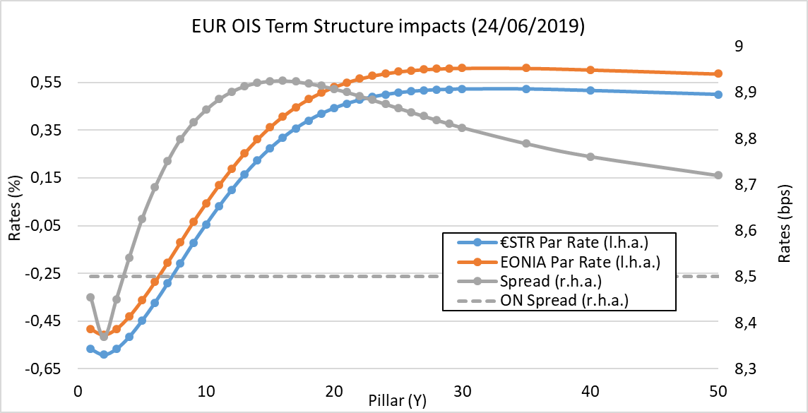
Figure 1: impact on OIS par rates. Left hand axis, continuous orange line: quoted EONIA OIS term structure as of 30/06/2020; continuous blue line: €STR OIS term structure built as described in sec. 3.1. Right hand axis, continuous grey line: spread between EONIA and €STR par rates; dashed grey line: 8.5 basis point constant spread between EONIA and €STR overnight rates.

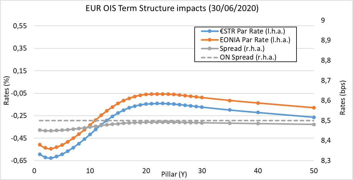
Figure 2: As in fig. 1, as of 30/06/2020.

As expected, according to eqs. (3.5)-(3.4), the spread between EONIA and €STR OIS par rates is not constant, but it depends on the level and shape of the term structure of EONIA OIS quotes. The difference with respect to the constant spread between EONIA and €STR overnight rates ($8.5$ bps) lies in the interval $[-0.2,+0.4]$ bps on the first date, an interval smaller than the typical market bid-ask spread of these instruments on the most liquid maturities (i.e. a couple of basis points). On the second date the difference is reduced by one order of magnitude (RMSE = $0.03$ bps versus RMSE = $0.34$ bps), quite below the bid-ask spread, due to the significant lowering of the EONIA OIS term structure. Part of this analysis is also reported in [21]. This result is consistent with eqs. (3.5)-(3.4) and with the small value of $8.5$ bps between €STR and EONIA overnight rates.

We conclude that the constant spread of $8.5$ bps between €STR and EONIA overnight rates does propagate to par OIS rates in a non-trivial way, but the residual distortion in the OIS term structure is quite small, depending on the level and shape of the market OIS par rates. As a consequence, one is allowed to bootstrap the €STR yield curve starting from EONIA OIS market quotes minus $8.5$ bps and, viceversa, bootstrap the EONIA yield curve starting from €STR OIS market quotes plus $8.5$ bps.

4 IRS Impacts

In this section we analyse the impacts of the transition from EONIA to €STR on EUR IRS instruments, indexed to EURIBOR. Looking at the pricing formulas in sec. 2.3 (eqs. (2.9), (2.10) and (2.12)), we recognize that the switch has both a direct and an indirect effect, as also discussed in detail in [21]. The direct effect is observable on IRSs subject to EONIA-discounting (because of either clearing rules, CSA rules or internal policy), due to the simple switch to €STR-discounting, keeping constant the forward rates (“constant forward rates approach”). The indirect effect is observable on EURIBOR forward rates because of the switch to €STR-discounting in the multi-curve bootstrapping procedure used to build the EURIBOR yield curves (see the discussion related to eq. (2.13)), keeping constant the market IRS par rates (“constant par rates approach”). We stress that the simultaneous switch of discounting curve both in pricing and in bootstrapping leads to a null impact on quoted par swap rates, since the bootstrapping procedure, by construction, fits the market quotes.

In the following sections we analyse both impacts, using an €STR-discounting curve produced from the theoretical €STR quotes obtained by shifting the market EUR OIS quotes by $-8.5$ bps, as discussed in sec. 3).

4.1 Constant Par Rates Approach

The constant par rate approach assumes that market EUR IRS par rates are not affected by the transition. As a consequence the quantities in IRS par rate formula (2.12) behaves as follows,

$$\begin{split}P^{\textit{EON}}(t;T_{i})&\longrightarrow P^{\textit{€ST}}(t;T_{i}),\quad i=\eta_{R}(t),\dots,n,\\ P^{\textit{EON}}(t;S_{j})&\longrightarrow P^{\textit{€ST}}(t;S_{j}),\quad j=\eta_{K}(t),\dots,m,\\ A(t;\textbf{S},\textit{EON})&\longrightarrow A(t;\textbf{S},\textit{€ST}),\\ F_{x,i}^{\textit{EON}}(t)&\longrightarrow F_{x,i}^{\textit{€ST}}(t),\quad i=\eta_{R}(t),\dots,n,\\ R_{x}(t;\textbf{T},\textbf{S},\textit{EON})&\longrightarrow R_{x}(t;\textbf{T},\textbf{S},\textit{€ST})=R_{x}(t;\textbf{T},\textbf{S},\textit{EON}).\\ \end{split}$$ (4.1)

We show in fig. 3 the differences between EONIA and €STR based EURIBOR 6M forward rates $F_{6M,i}^{\textit{EON}}(t)-F_{6M,i}^{\textit{€ST}}(t)$ up to $T=50Y$ for two different dates $t$ (total $100+100$ points). $F_{6M,i}^{\textit{EON}}(t)$ forward rates were computed from the EURIBOR 6M curve bootstrapped at time $t$ using EONIA-discounting, while $F_{6M,i}^{\textit{€ST}}(t)$ forward rates were computed from the EURIBOR 6M curve bootstrapped at time $t$ using €STR-discounting.

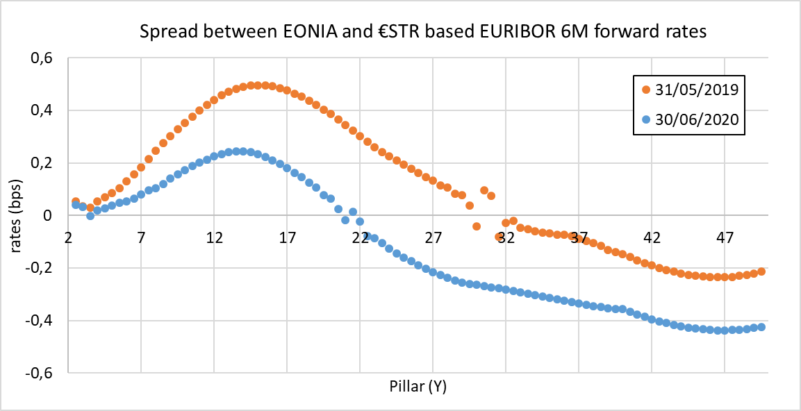
Figure 3: differences between EONIA and €STR based EURIBOR 6M forward rates $F_{6M,i}^{\textit{EON}}(t)-F_{6M,i}^{\textit{€ST}}(t)$ up to $T=50Y$, for $t=$31/5/2019 and $t=$30/6/2020. Minor irregularities are due to the interplay between yield curve shapes and interpolation effects.

The differences result to be quite small, lying in the interval $[-0.4,+0.5]$ bps, and their term structure and global amount remain stable for the two dates examined (RMSE = $0.27$ bps for both dates). We conclude that the indirect impacts under the constant par rates approach are negligible.

4.2 Constant Forward Rates Approach

The constant forward rate approach assumes that EURIBOR forward rates are not affected by the transition. As a consequence the quantities in IRS par rate formula (2.12) behaves as follows,

$$\begin{split}P^{\textit{EON}}(t;T_{i})&\longrightarrow P^{\textit{€ST}}(t;T_{i}),\quad i=\eta_{R}(t),\dots,n,\\ P^{\textit{EON}}(t;S_{j})&\longrightarrow P^{\textit{€ST}}(t;S_{j}),\quad j=\eta_{K}(t),\dots,m,\\ A(t;\textbf{S},\textit{EON})&\longrightarrow A(t;\textbf{S},\textit{€ST}),\\ F_{x,i}^{\textit{EON}}(t)&\longrightarrow F_{x,i}^{\textit{€ST}}(t)=F_{x,i}^{\textit{EON}}(t),\quad i=\eta_{R}(t),\dots,n,\\ R_{x}(t;\textbf{T},\textbf{S},\textit{EON})&\longrightarrow R_{x}(t;\textbf{T},\textbf{S},\textit{€ST}).\end{split}$$ (4.2)

We show in Fig. 4 the impact of the transition on par swap rates. In particular, we show market quotes for EURIBOR 6M IRS par rates (EONIA discounted) versus theoretical EURIBOR 6M IRS par rates (€STR discounted) computed using eq. (2.12), and their differences for two different dates.

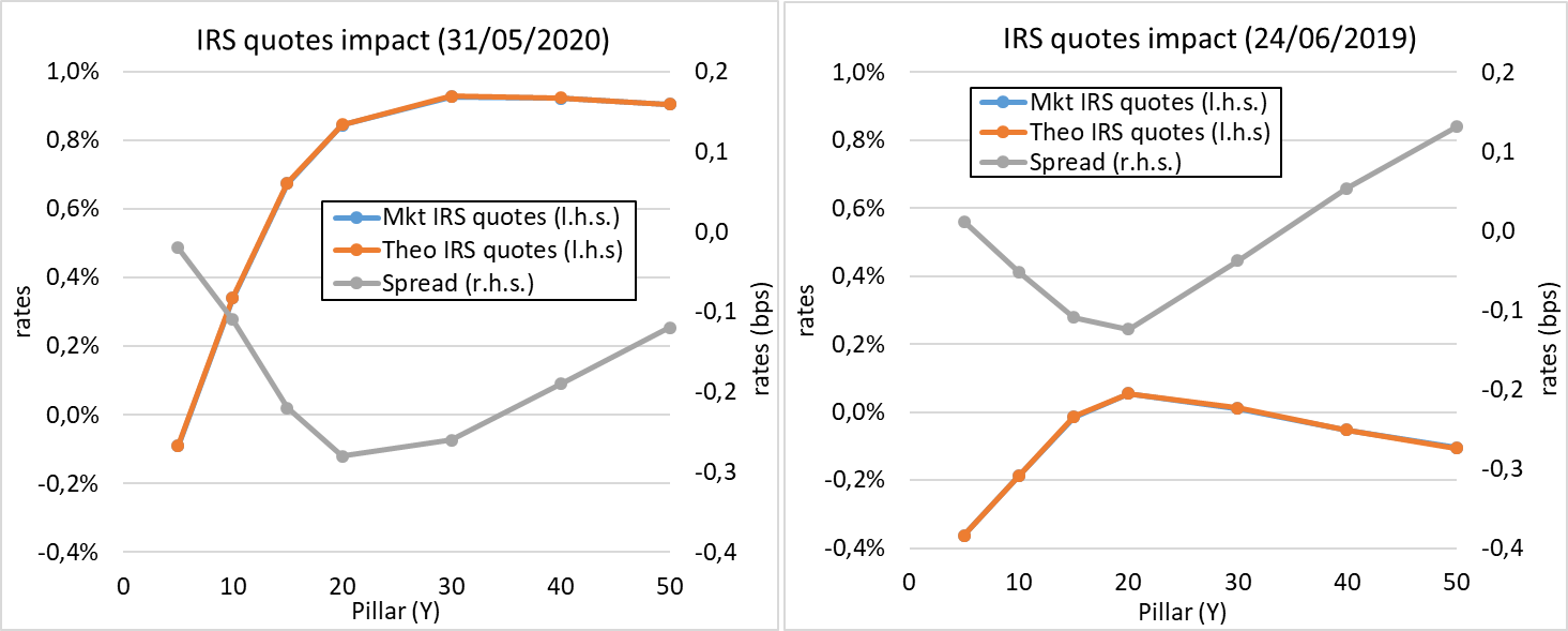
Figure 4: Discounting switch impacts on IRS par rates in the constant forward rates approach. Market IRS quotes (blue lines) refer to EURIBOR 6M IRS par rates (EONIA-discounting); theoretical quotes (orange lines) refer to EURIBOR 6M par rates in new €STR-discounting regime, obtained using EONIA based 6M EURIBOR forward rates; spreads (grey lines) refer to the differences between Market IRS quotes and theoretical quotes.

The differences result to be quite small, lying in the interval $[-0.3,+0.1]$ bps; moreover, on 30/06/2020 the differences were sensibly reduced (RMSE = $0.09$ bps versus RMSE = $0.19$ bps). Part of this analysis is also reported in [21].

Hence, also under the constant forward rate approach the impact of the discounting switch on IRS is negligible.

Overall, we conclude that the transition from EONIA to €STR overnight rates affects both par IRS rates and implied forward rates in a negligible way, also considering multi-curve bootstrapping. As a consequence, one may switch multi-curve bootstrapping of IBOR curves and IBOR-IRS pricing from EONIA to €STR quite safely. Furthermore, the adoption of a “clean discounting” approach, where counterparties agree to switch bilateral CSAs from EONIA to €STR flat and to switch the discount curve accordingly, is theoretically sound and practically feasible.

5 XVA Impacts

In this section we show that, assuming constant funding rates under the EONIA-€STR transition, the impact on the fair value $V(t)$ of an uncollateralised trade is greatly reduced by a compensation effect between the impacts on the base value $V_{0}(t)$ and on the $\mbox{{FVA}}(t)$.

5.1 Particular Case

We will proof the proposition above in the simplified situation outlined in sec. 2.4, using eq. (2.21), which is referred to a single cash flow received at time $T$ from a default free counterparty. According to eq. (2.1) and (2.21), the fair value of this trade is given, under EONIA-discounting, by

$$V^{\textit{EON}}(t)=V^{\textit{EON}}_{0}(t)+\mbox{{FVA}}^{\textit{EON}}(t)=P^{\textit{EON}}_{I}(t;T)C(T).$$ (5.1)

Let’s introduce the following zero rates,

$$\begin{split}R(t;T,\textit{EON})&=-\dfrac{1}{\tau(t;T)}\log P^{\textit{EON}}(t;T),\\ R_{I}(t;T,\textit{EON})&=-\dfrac{1}{\tau(t;T)}\log P_{I}^{\textit{EON}}(t;T),\\ \mathcal{S}_{I}(t,T,\textit{EON})&=R_{I}(t;T,\textit{EON})-R(t;T,\textit{EON}),\end{split}$$ (5.2)

where $\mathcal{S}_{I}$ is the funding zero spread. We assume here that the transition does not affect the Institution’s absolute funding level, i.e. that bonds and other funded instruments issued by $I$ maintain constant prices across the transition. Hence, the Institution’s funding (zero) rate $R_{I}(t;T,\textit{EON})$ remains constant across the transition, and the impact on the reference discount rate $R(t;T,\textit{EON})$ is absorbed by the corresponding impact on the funding spread $\mathcal{S}_{I}(t,T,\textit{EON})$. As a consequence the quantities in eqs. (5.2) above behaves as follows,

$$\begin{split}R(t;T,\textit{EON})&\longrightarrow R(t;T,\textit{€ST}),\\ R_{I}(t;T,\textit{EON})&\longrightarrow R_{I}(t;T,\textit{€ST})=R_{I}(t;T,\textit{EON}),\\ P^{\textit{EON}}(t;T)&\longrightarrow P^{\textit{€ST}}(t;T),\\ P_{I}^{\textit{EON}}(t;T)&\longrightarrow P_{I}^{\textit{€ST}}(t;T)=P_{I}^{\textit{EON}}(t;T),\\ \mathcal{S}_{I}(t,T,\textit{EON})&\longrightarrow\mathcal{S}_{I}(t,T,\textit{€ST}).\end{split}$$ (5.3)

Notice that the transformation of $S_{I}$ in eq. (5.3) leads to

$$\mathcal{S}_{I}(t,T,\textit{€ST}) =R_{I}(t;T,\textit{€ST})-R(t;T,\textit{€ST})$$

$$=\mathcal{S}_{I}(t,T,\textit{EON})-\left[R(t;T,\textit{€ST})-R(t;T,\textit{EON})\right]\approx\mathcal{S}_{I}(t,T,\textit{EON})-\Delta,$$ (5.4)

where the last equality is obtained from

$$R(t;T,\textit{€ST})-R(t;T,\textit{EON})=\dfrac{1}{\tau(t;T)}\log\dfrac{P^{\textit{EON}}(t;T)}{P^{\textit{€ST}}(t;T)}=\dfrac{1}{\tau(t;T)}\log\dfrac{\mathbb{E}_{t}^{\mathbb{Q}}\left[e^{-\int_{t}^{T}r_{\textit{EON}}(u)\,du}\right]}{\mathbb{E}_{t}^{\mathbb{Q}}\left[e^{-\int_{t}^{T}r_{\textit{€ST}}(u)\,du}\right]}\\ =\dfrac{1}{\tau(t;T)}\log\dfrac{\mathbb{E}_{t}^{\mathbb{Q}}\left[e^{-\int_{t}^{T}r_{\textit{EON}}(u)\,du}\right]}{\mathbb{E}_{t}^{\mathbb{Q}}\left[e^{-\int_{t}^{T}\left[r_{\textit{EON}}(u)+\Delta\right]\,du}\right]}=\dfrac{1}{\tau(t;T)}\log e^{\Delta(T-t)}=\Delta\dfrac{(T-t)}{\tau(t;T)}\approx\Delta.$$ (5.5)

The result in eq. (5.5) above is also reported in [17]. We notice that possible different conventions for spread and zero rate year fractions could lead to an approximate equivalence. Using eq. (5.3), the fair value in eq. (5.1) becomes

$$\begin{split}V^{\textit{EON}}(t)=P_{I}^{\textit{EON}}(t;T)C(T)\longrightarrow P_{I}^{\textit{€ST}}(t;T)C(T)=P_{I}^{\textit{EON}}(t;T)C(T)=V^{\textit{EON}}(t),\end{split}$$ (5.6)

i.e., the fair value is constant across the transition.

The exact result proved above can be generalised to a collection of fixed positive cash flows (e.g. the fixed leg of receiver IRS), since the simplified FVA formula in eq. (2.21) still holds for each single cash flow.

We conclude that, under appropriate hypotheses, the impact of EONIA-€STR transition on the fair value $V$ of a trade is null, since the impact of the discounting switch on the base value $V_{0}$ is balanced by the corresponding impact on the FVA.

5.2 General Case

In the general case of multiple stochastic cash flows with defaultable counterparties the XVAs formulas are more complex (see e.g. [10, 11]) and the simple proof given in the previous sec. 5.1 is no longer straightforward. In any case, guided by the simplified case, we may still leverage on the impacts analysed in sec. 3 to understand qualitatively the impacts of the EONIA to €STR transition, as follows.

CVA:

it is a negative adjustment dependent on the Expected Positive Exposure (EPE) $\longrightarrow$ it is affected by a negative impact (CVA becomes more negative).

DVA:

it is a positive adjustment dependent on the Expected Negative Exposure (ENE) $\longrightarrow$ it is affected by a positive impact (DVA becomes more positive).

FVA:

it is a negative adjustment dependent on the Expected Positive Exposure (EPE) $\longrightarrow$ it is affected by a negative impact (FVA becomes more negative, as for CVA); furthermore, the FVA is also dependent on the funding spread $S_{I}$ $\longrightarrow$ it is affected by another negative impact.

We conclude that the impact of the transition on FVA is larger than for CVA and DVA, hence the cancellation effect between the FVA and the base value $V_{0}$ across the transition discussed in the previous sec. 5.1 still exists. Notice that trades with negative exposure generate a positive impact.

The discussion above actually depends on the XVAs management practice of Institutions, which is known to be quite diversified both in the selection of which XVAs are accounted at fair value and in the construction of own credit and funding curves (see e.g. [22]). We included CVA, DVA FVA (FCA actually) and we discarded the FBA, MVA and KVA, but this is only one possible choice. Hence, the exact conclusions regarding the impact of the EONIA to €STR transition should be carefully examined by each Institution according to its internal XVAs policy.

6 Conclusions

We have shown in detail how the transition from EONIA to €STR overnight rates affects the pricing of OIS, IRS and their associated XVAs, and what are the consequences on cleared, collateralised and non-collateralised linear financial instruments, both from a theoretical and numerical point of view.

In particular, we have shown that the constant spread of $8.5$ bps between €STR and EONIA overnight rates does propagate to par OIS rates in a non-trivial way, but the residual distortion in the OIS term structure is quite small, depending on the level and shape of the market OIS par rates. As a consequence, the differences between market quotes of €STR and EONIA OIS are expected to amount to $8.5$ bps, except in case of illiquidity problems, and one is allowed to safely bootstrap the €STR yield curve starting from EONIA OIS market quotes minus $8.5$ bps or, viceversa, bootstrap the EONIA yield curve starting from €STR OIS market quotes plus $8.5$ bps. These yield curves can be used to price EUR OIS indexed to EONIA or €STR. They can also be used as discounting curves for any kind of trade, consistently with either EONIA or €STR collateral.

Regarding IRS, we have shown that the transition from EONIA to €STR overnight rates affects both par IRS rates and implied EURIBOR forward rates in a negligible way, also considering multi-curve bootstrapping. As a consequence, one may safely switch multi-curve bootstrapping of EURIBOR curves and EURIBOR IRS pricing from EONIA to €STR.

Finally, we have shown that the impact of the transition from EONIA to €STR on non-collateralised trades is greatly reduced, since changes in the base value tends to be counter-balanced by corresponding changes on Funding Value Adjustment (i.e. its negative component of Funding Cost Adjustment).

The combination of the three findings above makes theoretically sound and safe the adoption of the “clean discounting” approach recommended by the ECB [2], EONIA-free and based on €STR only, to any trade: cleared, under bilateral CSA, non-collateralised, with a limited impact. Such conclusion is valid at least for linear IR derivatives, which cover most of the trading volume and existing positions in the EUR market. Analyses for non-linear IR derivatives can be found e.g. in [23, 24]. Hence, after the EONIA to €STR switch performed on 27th July 2020 by Central Counterparties for cleared derivatives, the financial industry may safely proceed to switch both bilateral collateral agreements covering non-cleared EUR OTC derivatives, and, consistently, non-collateralised OTC derivatives including XVAs. Such EONIA-free pricing framework is essential for the complete elimination of EONIA before its discontinuation on 31st December 2021.

Appendix A OIS Details

A.1 Discrete Compounding

We compute the €STR forward overnight compounded rate $F_{\textit{€ST,i}}(t)$ expected at time at time $t<T_{i}$ for the future OIS floating coupon period $\left[T_{i-1},T_{i}\right]$ as the expectation of the corresponding spot rate in eq. (3.2) under the $T_{i}-$forward measure, using the forward measure equivalence $\mathbb{Q}^{\textit{€ST}}_{T_{i}}\sim\mathbb{Q}^{\textit{EON}}_{T_{i}}$ discussed in sec. 2.2,

$$\begin{split}F_{\textit{€ST,i}}(t)&=\mathbb{E}_{t}^{\mathbb{Q}^{\textit{€ST}}_{T_{i}}}\left[R_{\textit{€ST}}(T_{i-1},T_{i})\right]=\mathbb{E}_{t}^{\mathbb{Q}^{\textit{EON}}_{T_{i}}}\left[R_{\textit{€ST}}(T_{i-1},T_{i})\right]\\ &=\frac{1}{\tau_{i}}\mathbb{E}_{t}^{\mathbb{Q}^{\textit{EON}}_{T_{i}}}\left\{\prod_{k=1}^{n_{i}}\left[1+\left[R_{\textit{EON}}(T_{i,k-1},T_{i,k})+\Delta\right]\tau_{i,k}\right]-1\right\}\\ &=\frac{1}{\tau_{i}}\left\{\prod_{k=1}^{n_{i}}\left[1+\left[\mathbb{E}_{t}^{\mathbb{Q}^{\textit{EON}}_{T_{i,k}}}\left[R_{\textit{EON}}(T_{i,k-1},T_{i,k})\right]+\Delta\right]\tau_{i,k}\right]-1\right\}\\ &=\frac{1}{\tau_{i}}\left\{\prod_{k=1}^{n_{i}}\left[1+\left[F_{\textit{EON,i,k}}(t)+\Delta\right]\tau_{i,k}\right]-1\right\}\\ &=\frac{1}{\tau_{i}}\left\{\prod_{k=1}^{n_{i}}\left[\frac{P^{\textit{EON}}(t;T_{i,k-1})}{P^{\textit{EON}}(t;T_{i,k})}+\Delta\,\tau_{i,k}\right]-1\right\},\end{split}$$ (A.1)

(see e.g. [18, 19] for detailed math), where $F_{\textit{EON,i,k}}(t)$ is the forward overnight rate observed at time $t$ for the future overnight period $\left[T_{i,k-1},T_{i,k}\right]$, a martingale under the $T_{i,k}-$ forward measure $\mathbb{Q}_{T_{i,k}}$ given in eq. (2.13). In eq. A.1 we assumed $\tau_{F,i,k}=\tau_{i,k}\;\forall\;i,k$. The product in the last row of eq. (A.1) may be manipulated as follows,

$$\prod_{k=1}^{n_{i}}\left\{\frac{P^{\textit{EON}}(t;T_{i,k-1})}{P^{\textit{EON}}(t;T_{i,k})}+\Delta\,\tau_{i,k}\right\}\\ =\left[\frac{P^{\textit{EON}}(t;T_{i,0})}{P^{\textit{EON}}(t;T_{i,1})}+\Delta\,\tau_{i,1}\right]\cdot\left[\frac{P^{\textit{EON}}(t;T_{i,1})}{P^{\textit{EON}}(t;T_{i,2})}+\Delta\,\tau_{i,2}\right]\cdots\left[\frac{P^{\textit{EON}}(t;T_{i,n_{i-1}})}{P^{\textit{EON}}(t;T_{i,n_{i}})}+\Delta\,\tau_{i,n_{i}}\right]\\ =\prod_{k=1}^{n_{i}}\frac{P^{\textit{EON}}(t;T_{i,k-1})}{P^{\textit{EON}}(t;T_{i,k})}+\Delta\sum_{l=1}^{n_{i}}\tau_{i,l}\prod_{\begin{subarray}{c}k=1\\ k\neq l\end{subarray}}^{n_{i}}\frac{P^{\textit{EON}}(t;T_{i,k-1})}{P^{\textit{EON}}(t;T_{i,k})}+f\left[\textit{O}(\Delta^{m},m\geq 2)\right],$$ (A.2)

where $f$ gathers the remaining terms of order $m\geq 2$ in the spread $\Delta$, which can be neglected. The second term in eq. (A.2) can be written as follows,

$$\Delta\sum_{l=1}^{n_{i}}\tau_{i,l}\prod_{\begin{subarray}{c}k=1\\ k\neq l\end{subarray}}^{n_{i}}\frac{P^{\textit{EON}}(t;T_{i,k-1})}{P^{\textit{EON}}(t;T_{i,k})}=\Delta\sum_{l=1}^{n_{i}}\tau_{i,l}\frac{P^{\textit{EON}}(t;T_{i,l})}{P^{\textit{EON}}(t;T_{i,l-1})}\prod_{k=1}^{n_{i}}\frac{P^{\textit{EON}}(t;T_{i,k-1})}{P^{\textit{EON}}(t;T_{i,k})}.$$ (A.3)

Hence, considering the telescopic product

$$\prod_{k=1}^{n_{i}}\frac{P^{\textit{EON}}(t;T_{i,k-1})}{P^{\textit{EON}}(t;T_{i,k})}=\frac{P^{\textit{EON}}(t;T_{i,0})}{P^{\textit{EON}}(t;T_{i,n_{i}})}=\frac{P^{\textit{EON}}(t;T_{i-1})}{P^{\textit{EON}}(t;T_{i})},$$ (A.4)

eq. (A.1) becomes

$$F_{\textit{€ST,i}}(t) \approx\frac{1}{\tau_{i}}\left[\frac{P^{\textit{EON}}(t;T_{i-1})}{P^{\textit{EON}}(t;T_{i})}+\Delta\frac{P^{\textit{EON}}(t;T_{i-1})}{P^{\textit{EON}}(t;T_{i})}\sum_{l=1}^{n_{i}}\tau_{i,l}\frac{P^{\textit{EON}}(t;T_{i,l})}{P^{\textit{EON}}(t;T_{i,l-1})}-1\right]$$

$$=F_{\textit{EON,i}}(t)+\Sigma_{d,i}(\Delta),$$ (A.5)

$$\Sigma_{d,i}(\Delta) :=\frac{\Delta}{\tau_{i}}\left[\frac{P^{\textit{EON}}(t;T_{i-1})}{P^{\textit{EON}}(t;T_{i})}\sum_{l=1}^{n_{i}}\tau_{i,l}\frac{P^{\textit{EON}}(t;T_{i,l})}{P^{\textit{EON}}(t;T_{i,l-1})}\right].$$ (A.6)

Eq. (A.5) allows to express the €STR forward overnight compounded rate as the EONIA forward overnight compounded rate plus the spread in eq. (A.6). Hence, the price a €STR OIS is given, using eq. (2.9), by

$$\mbox{{OIS}}_{\textit{€ST}}(t;\bm{T},\bm{S},K,\omega,\alpha)=\omega N\left[\sum_{i=\eta_{R}(t)}^{n}P^{\alpha}(t;T_{i})F_{\textit{€ST,i}}(t)\tau_{R,i}-KA(t;\bm{S},\alpha)\right],\\ =\omega N\left\{\sum_{i=\eta_{R}(t)}^{n}\left[P^{\alpha}(t;T_{i})F_{\textit{EON,i}}(t)\tau_{R,i}+P^{\alpha}(t;T_{i})\Sigma_{d,i}(\Delta)\tau_{R,i}\right]-KA(t;\bm{S},\alpha)\right\},\\ =\mbox{{OIS}}_{\textit{EON}}(t;\bm{T},\bm{S},K,\omega,\alpha)+\omega N\sum_{i=\eta_{R}(t)}^{n}P^{\alpha}(t;T_{i})\Sigma_{d,i}(\Delta)\tau_{R,i}.$$ (A.7)

The €ST OIS par rate is obtained by setting $\mbox{{OIS}}_{\textit{€ST}}(t;\bm{T},\bm{S},K,\omega,\alpha)=0$ and solving for $K$. The result is given in eq. (3.5).

A.2 Continuous Compounding

If we consider the limit for $\tau_{i,k}\rightarrow 0$, we can write (3.2) as

$$\begin{split}R_{\textit{€ST}}(T_{i-1},T_{i})&\approx\dfrac{1}{\tau_{i}}\left[e^{\int_{T_{i-1}}^{T_{i}}r_{\textit{€ST}}(u)du}-1\right]\\ &=\dfrac{1}{\tau_{i}}\left[e^{\int_{T_{i-1}}^{T_{i}}[r_{\textit{EON}}(u)+\Delta]du}-1\right]\\ &=\dfrac{1}{\tau_{i}}\left[e^{\Delta\tau_{i}}e^{\int_{T_{i-1}}^{T_{i}}r_{\textit{EON}}(u)du}-1\right].\end{split}$$ (A.8)

As in the discrete case (eq. (A.1)), we compute the forward rate,

$$F_{\textit{€ST,i}}(t) :=\mathbb{E}_{t}^{\mathbb{Q}_{T_{i}}}\left[R_{\textit{€ST}}(T_{i-1},T_{i})\right]$$

$$=\dfrac{1}{\tau_{i}}\left\{e^{\Delta\tau_{i}}\mathbb{E}_{t}^{\mathbb{Q}_{T_{i}}}\left[e^{\int_{T_{i-1}}^{T_{i}}r_{\textit{EON}}(u)du}\right]-1\right\}$$

$$=\dfrac{1}{\tau_{i}}\left\{e^{\Delta\tau_{i}}\dfrac{1}{P^{\textit{EON}}(t;T_{i})}\mathbb{E}_{t}^{\mathbb{Q}}\left[e^{-\int_{t}^{T_{i}}r_{\textit{EON}}(u)du}e^{\int_{T_{i-1}}^{T_{i}}r_{\textit{EON}}(u)du}\right]-1\right\}$$

$$=\dfrac{1}{\tau_{i}}\left\{e^{\Delta\tau_{i}}\dfrac{1}{P^{\textit{EON}}(t;T_{i})}\mathbb{E}_{t}^{\mathbb{Q}}\left[e^{-\int_{t}^{T_{i-1}}r_{\textit{EON}}(u)du}\right]-1\right\}$$

$$=\dfrac{1}{\tau_{i}}\left[e^{\Delta\tau_{i}}\dfrac{P^{\textit{EON}}(t;T_{i-1})}{P^{\textit{EON}}(t;T_{i})}-1\right],$$

$$=\dfrac{1}{\tau_{i}}\left[\dfrac{P^{\textit{EON}}(t;T_{i-1})}{P^{\textit{EON}}(t;T_{i})}-1\right]+\dfrac{1}{\tau_{i}}\left(e^{\Delta\tau_{i}}-1\right)\dfrac{P^{\textit{EON}}(t;T_{i-1})}{P^{\textit{EON}}(t;T_{i})}$$

$$=F_{\textit{EON,i}}(t)+\Sigma_{c,i}$$ (A.9)

$$\Sigma_{c,i} =\dfrac{1}{\tau_{i}}\dfrac{P^{\textit{EON}}(t;T_{i-1})}{P^{\textit{EON}}(t;T_{i})}\left(e^{\Delta\tau_{i}}-1\right)$$ (A.10)

where we switched from $T_{i}-$forward measure $\mathbb{Q}_{T_{i}}$ to risk neutral measure $\mathbb{Q}$. As in discrete case discussed in sec. A.1, eq. (A.9) allows to express the €STR forward overnight compounded rate as the EONIA forward overnight compounded rate plus the spread in eq. (A.10). Hence, the price a €STR OIS is given, using eq. (2.9), by

$$\mbox{{OIS}}_{\textit{€ST}}(t;\bm{T},\bm{S},K,\omega,\alpha)=\omega N\left[\sum_{i=\eta_{R}(t)}^{n}P^{\alpha}(t;T_{i})F_{\textit{€ST,i}}(t)\tau_{R,i}-KA(t;\bm{S},\alpha)\right],\\ =\omega N\left\{\sum_{i=\eta_{R}(t)}^{n}\left[P^{\alpha}(t;T_{i})F_{\textit{EON,i}}(t)\tau_{R,i}+P^{\alpha}(t;T_{i})\Sigma_{c,i}(\Delta)\tau_{R,i}\right]-KA(t;\bm{S},\alpha)\right\},\\ =\mbox{{OIS}}_{\textit{EON}}(t;\bm{T},\bm{S},K,\omega,\alpha)+\omega N\sum_{i=\eta_{R}(t)}^{n}P^{\alpha}(t;T_{i})\Sigma_{c,i}(\Delta)\tau_{R,i}.$$ (A.11)

The €ST OIS par rate is obtained by setting $\mbox{{OIS}}_{\textit{€ST}}(t;\bm{T},\bm{S},K,\omega,\alpha)=0$ and solving for $K$. The result is given in eq. (3.10).

Appendix B Risky ZCB details

B.1 Hazard rate

The hazard rate $\gamma=\gamma(t)$ referred to the default time process $\tau$ is defined as

$$\gamma(t)dt=\mathbb{Q}(t<\tau\leq t+dt|\tau>t)$$ (B.1)

that is the probability that default occurs within the interval $\mathopen{(}t,t+dt\mathclose{]}$, conditioned to the fact that the default has not already occurred at $t$; using conditioned probability definition, we may write

$$\mathbb{Q}(t<\tau\leq t+dt)=\gamma(t)\mathbb{Q}(\tau>t)dt$$ (B.2)

and then

$$\begin{split}\mathbb{Q}(t<\tau\leq t+dt|\tau>t)&=\mathbb{Q}({\color[rgb]{0,0,0}\{\tau\leq t+dt\}}\cap{\color[rgb]{0,0,0}\{\tau>t\}})\\ &=\mathbb{Q}(\{\tau>t\}\setminus\{\tau>t+dt\})\\ &=\mathbb{Q}(\tau>t)-\mathbb{Q}(\tau>t+dt).\end{split}$$ (B.3)

Setting $\Gamma(t):=\mathbb{Q}(\tau>t)$ we get

$$\Gamma(t)-\Gamma(t+dt)=\gamma(t)\Gamma(t)dt$$ (B.4)

$$\Gamma^{\prime}(t)=-\gamma(t)\Gamma(t).$$ (B.5)

Hence we obtain the following expression for the survival probability

$$\mathbb{Q}(\tau>t)=\Gamma(t)=e^{-\int_{0}^{t}\gamma(s)ds}.$$ (B.6)

The derivation above assumes $\gamma$ deterministic. According to [14] for $\gamma$ stochastic we have

$$\mathbb{Q}(\tau>t):=\mathbb{E}^{\mathbb{Q}}\left[\mathds{1}_{\{\tau>T\}}\Big{|}\mathcal{H}_{t}\right]=\mathbb{E}^{\mathbb{Q}}\left[e^{-\int_{0}^{t}\gamma(s)ds}\Big{|}\mathcal{H}_{t}\right]:=S(0;t).$$ (B.7)

B.2 Risky Zero Coupon Bond

We define the risky zero coupon bond with no recovery rate as the bond issued by a defaultable issuer $I$ paying one unit of currency at maturity $T$ if the issuer $I$ has not defaulted before. The price at time $t<T$ is given by a generalization of eq. (2.4),

$$\begin{split}P_{I}(t;T)=\mathbb{E}^{\mathbb{Q}}\left[D(t;T)\bm{1}_{\left\{\tau_{I}>T\right\}}|\mathcal{G}_{t}\right],\end{split}$$ (B.8)

where $\tau_{I}>t$ is the (stochastic) default time of the issuer. If interest rates and default time are independent of each other we obtain, using eq. B.7,

$$P_{I}(t;T)=\mathbb{E}^{\mathbb{Q}}\left[D(t;T)|\mathcal{F}_{t}\right]\mathbb{E}^{\mathbb{Q}}\left[\bm{1}_{\left\{\tau_{I}>T\right\}}|\mathcal{H}_{t}\right]\\ =P(t;T)S_{I}(t;T)=\mathbb{E}^{\mathbb{Q}}\left[e^{-\int_{t}^{T}\left[r(s)+\gamma_{I}(s)\right]ds}\Big{|}\mathcal{F}_{t}\right],$$ (B.9)

where $S_{I}(t,T)$ is the survival probabiliy for $I$ until time $T$, evaluated in $t$, and $\gamma$ is the hazard rate defined in sec. B.1.

Let’s now consider the more realistic case where recovery rate is represented by a non-null process $\mathcal{R}_{I}$. It can be shown (see [25, 26]) that the price of a risky zero coupon bond becomes

$$\begin{split}P_{I}(t;T)&=\mathbb{E}_{t}^{\mathbb{Q}}\left[D(t;\tau_{I})\mathcal{R}(\tau_{I})\mathds{1}_{\{\tau_{I}\leq T\}}+D(t;T)\mathds{1}_{\{\tau_{I}>T\}}\right]\\ &=\mathbb{E}_{t}^{\mathbb{Q}}\left[\int_{t}^{T}\mathcal{R}_{I}(u)\gamma_{I}(u)e^{-\int_{t}^{u}\left[r(s)+\gamma_{I}(s)\right]ds}du\right]+P_{I}(t;T).\end{split}$$ (B.10)

We adopt the recovery of treasury model ([25, 26]), such that

$$\mathcal{R}_{I}(t)=\textit{Rec}_{I}\,P(t;T),$$ (B.11)

where $\textit{Rec}_{I}$ is a constant. Under such model the price of the risky zero coupon bond in eq. (B.10) simplifies as

$$\begin{split}P_{I}(t;T)&=\textit{Rec}_{I}\mathbb{E}_{t}^{\mathbb{Q}}\left[\int_{t}^{T}P(u,T)\gamma_{I}(u)e^{-\int_{t}^{u}\left[r(s)+\gamma_{I}(s)\right]ds}du\right]+P_{I}(t;T)\\ &=\textit{Rec}_{I}\mathbb{E}_{t}^{\mathbb{Q}}\left[D(t;T)\int_{t}^{T}\gamma_{I}(u)e^{-\int_{t}^{u}\gamma_{I}(s)ds}du\right]+P_{I}(t;T)\\ &=\textit{Rec}_{I}\mathbb{E}_{t}^{\mathbb{Q}}\left[D(t;T)\left(1-e^{-\int_{t}^{T}\gamma_{I}(s)ds}\right)\right]+P_{I}(t;T)\\ &=\textit{Rec}_{I}\left[P(t;T)-P_{I}(t;T)\right]+P_{I}(t;T)\\ &=P(t;T)\left[\textit{Rec}_{I}+(1-\textit{Rec}_{I})S_{I}(t,T)\right].\end{split}$$ (B.12)

B.3 Funding Spread

The zero funding spread rate defined in eq. (5.2) can be written as

$$\mathcal{S}_{I}(t,T)=\dfrac{1}{T-t}\log\dfrac{P(t;T)}{P_{I}(t,T)}.$$ (B.13)

Using eq. (B.12) above we obtain

$$\begin{split}\mathcal{S}_{I}(t,T)&=\dfrac{1}{T-t}\log\dfrac{1}{1-(1-\textit{Rec}_{I})\left[1-S_{I}(t,T)\right]}\\ &=-\dfrac{1}{T-t}\log\left\{1-(1-\textit{Rec}_{I})\left[1-S_{I}(t,T)\right]\right\}\\ &=-\dfrac{1}{T-t}\log\left[1-1+S_{I}(t,T)+\textit{Rec}_{I}-\textit{Rec}_{I}S_{I}(t,T)\right]\\ &=-\dfrac{1}{T-t}\log\left\{S_{I}(t,T)\left[1+\textit{Rec}_{I}\left(-1+\dfrac{1}{S_{I}(t,T)}\right)\right]\right\}.\end{split}$$ (B.14)

We now recall that the survival probability may be defined through the hazard rate (define in sec B.1)

$$S_{I}(t,T)=e^{-\int_{t}^{T}\gamma(s)ds}.$$ (B.15)

Inserting the survivial probability (B.15) inside the spread rate formula (B.14), we arrive to (see [27], [25])

$$\begin{split}\mathcal{S}(t,T)&=\dfrac{\int_{t}^{T}\gamma(s)ds}{T-t}-\dfrac{1}{T-t}\log\left[1+\textit{Rec}_{I}\left(e^{\int_{t}^{T}\gamma(s)ds}-1\right)\right].\end{split}$$ (B.16)

In order to obtain the short spread rate, we apply the limit

$$\begin{split}s_{I}(t):=\lim_{T\rightarrow t^{+}}\mathcal{S}(t,T)=\gamma(t)(1-\textit{Rec}_{I}).\end{split}$$ (B.17)

Using eq. (B.5) we finally obtain

$$s_{I}(u)=-\dfrac{\partial_{u}S_{I}(t,u)}{S_{I}(t,u)}(1-\textit{Rec}_{I}).$$ (B.18)

References

- [1] Financial Stability Board. Reforming Major Interest Rate Benchmarks. July 2014. https://www.fsb.org/2014/07/r_140722/.
- [2] European Central Bank. Recommendations of the working group on euro risk-free rates on the transition path from EONIA to the €STR and on a €STR-based forward-looking term structure methodology. March 2019. https://www.ecb.europa.eu/pub/pdf/annex/ecb.sp190314_annex_recommendation.en.pdf.
- [3] Regulation (EU) 2016/1011 of the European Parliament and of the Council of 8 June 2016 on indices used as benchmarks in financial instruments and financial contracts or to measure the performance of investment funds and amending Directives 2008/48/EC and 2014/17/EU and Regulation (EU) No 596/2014. June 2016. https://eur-lex.europa.eu/legal-content/EN/TXT/?uri=CELEX%3A32016R1011.
- [4] Euro OverNight Index Average (EONIA) rate. https://www.emmi-benchmarks.eu/euribor-eonia-org/about-eonia.html.
- [5] Euro OverNight Index Average (EONIA) rate. https://www.emmi-benchmarks.eu/euribor-org/about-euribor.html.
- [6] Working group on euro risk-free rates. https://www.ecb.europa.eu/paym/initiatives/interest_rate_benchmarks/WG_euro_risk-free_rates/html/index.en.html.
- [7] European Central Bank. Overview of the euro short-term rate (€STR). https://www.ecb.europa.eu/stats/financial_markets_and_interest_rates/euro_short-term_rate/html/eurostr_overview.en.html.
- [8] European Central Bank. The euro short-term rate €STR methodology and policies. June 2018. https://www.ecb.europa.eu/paym/initiatives/interest_rate_benchmarks/shared/pdf/ecb.ESTER_methodology_and_policies.en.pdf.
- [9] Damiano Brigo and Andrea Pallavicini. CCPs, Central Clearing, CSA, Credit Collateral and Funding Costs Valuation FAQ: Re-Hypothecation, CVA, Closeout, Netting, WWR, Gap-Risk, Initial and Variation Margins, Multiple Discount Curves, FVA? SSRN eLibrary, December 2013.
- [10] Andrew Green. XVA: Credit, Funding and Capital Valuation Adjustment. Wiley Finance. John Wiley & Sons, November 2015.
- [11] Jon Gregory. The Xva Challenge: Counterparty Risk, Funding, Collateral, Capital and Initial Margin. Wiley Finance. John Wiley & Sons Inc, April 2020.
- [12] Vladimir V. Piterbarg. Cooking With Collateral. Risk Magazine, August 2012.
- [13] Damiano Brigo, Cristin Buescu, Marco Francischiello, Andrea Pallavicini, and Marek Rutkowski. Risk-Neutral Valuation Under Differential Funding Costs, Defaults and Collateralization. SSRN eLibrary, February 2018.
- [14] Damiano Brigo and Fabio Mercurio. Interest-Rate Models - Theory and Practice. Springer, 2nd edition, 2006.
- [15] Regulation (eu) no 575/2013 of the european parliament and of the council of 26 june 2013 on prudential requirements for credit institutions and investment firms and amending regulation (eu) no 648/2012. Official Journal of the European Union, June 2013.
- [16] Vladimir V. Piterbarg. Funding Beyond Discounting: Collateral Agreements and Derivatives Pricing. Risk Magazine, February 2010.
- [17] European Central Bank. Report by the working group on euro risk-free rates on the risk management implications of the transition from EONIA to the €STR and the introduction of €STR-based fallbacks for EURIBOR. October 2019. https://www.ecb.europa.eu/pub/pdf/other/ecb.wgeurofr_riskmanagementimplicationstransitioneoniaeurostrfallbackseuribor~156067d893.en.pdf.
- [18] Ferdinando M. Ametrano and Marco Bianchetti. Everything You Always Wanted to Know About Multiple Interest Rate Curve Bootstrapping but Were Afraid to Ask. SSRN eLibrary, April 2013.
- [19] Marc Henrard. Interest rate modelling in the multi-curve framework: Foundations, evolution and implementation. Springer, 2014.
- [20] Massimo Morini. Solving the Puzzle in the Interest Rate Market. SSRN working paper, 2009.
- [21] European Central Bank. Report by the working group on euro risk-free rates on the impact of the transition from EONIA to the €STR on cash and derivatives products. August 2019. https://www.ecb.europa.eu/pub/pdf/other/ecb.wgeurorfr_impacttransitioneoniaeurostrcashderivativesproducts~d917dffb84.en.pdf.
- [22] XVA Special report. Risk, 2019.
- [23] Vladimir Piterbarg. Interest rates benchmark reform and options markets. Available at SSRN, February 2020.
- [24] European Central Bank. Recommendation by the working group on euro risk-free rates on swaptions affected by the central clearing counterparties’ discounting transition from EONIA to €STR. June 2020. https://www.ecb.europa.eu/pub/pdf/other/ecb.recommendation_swaptions_impacted_by_discounting_switch_to_EuroSTR~a64f042ed9.en.pdf?be826ce2f0f27c70fd252d2e2cc5483a.
- [25] Tomasz R Bielecki and Marek Rutkowski. Credit risk: modeling, valuation and hedging. Springer Science & Business Media, 2013.
- [26] Matheus Grasselli and Thomas Hurd. Interest rate and credit risk modeling. Hamilton: McMaster University., 2015. https://ms.mcmaster.ca/~grasselli/Credittext2015.pdf.
- [27] Robert A Jarrow, David Lando, and Stuart M Turnbull. A markov model for the term structure of credit risk spreads. The review of financial studies, 10(2):481–523, 1997.