Bypassing orthogonalization in
the quantum DPP sampler

Abstract

Given an $n\times r$ matrix $X$ of rank $r$, consider the problem of sampling $r$ integers $\mathtt{C}\subset\{1,\dots,n\}$ with probability proportional to the squared determinant of the rows of $X$ indexed by $\mathtt{C}$. The distribution of $\mathtt{C}$ is called a projection determinantal point process (DPP). The vanilla classical algorithm to sample a DPP works in two steps, an orthogonalization in $\mathcal{O}(nr^{2})$ and a sampling step of the same cost. The bottleneck of recent quantum approaches to DPP sampling remains that preliminary orthogonalization step. For instance, (Kerenidis and Prakash, 2022) proposed an algorithm with the same $\mathcal{O}(nr^{2})$ orthogonalization, followed by a $\mathcal{O}(nr)$ classical step to find the gates in a quantum circuit. The classical $\mathcal{O}(nr^{2})$ orthogonalization thus still dominates the cost. Our first contribution is to reduce preprocessing to normalizing the columns of $X$, obtaining $\mathsf{X}$ in $\mathcal{O}(nr)$ classical operations. We show that a simple circuit inspired by the formalism of Kerenidis et al., 2022 samples a DPP of a type we had never encountered in applications, which is different from our target DPP. Plugging this circuit into a rejection sampling routine, we recover our target DPP after an expected $1/\det\mathsf{X}^{\top}\mathsf{X}=1/a$ preparations of the quantum circuit. Using amplitude amplification, our second contribution is to boost the acceptance probability from $a$ to $1-a$ at the price of a circuit depth of $\mathcal{O}(r\log n/\sqrt{a})$ and $\mathcal{O}(\log n)$ extra qubits. Prepending a fast, sketching-based classical approximation of $a$, we obtain a pipeline to sample a projection DPP on a quantum computer, where the former $\mathcal{O}(nr^{2})$ preprocessing bottleneck has been replaced by the $\mathcal{O}(nr)$ cost of normalizing the columns and the cost of our approximation of $a$.

Keywords— Determinantal point processes, free fermions, quantum circuits.

1 Introduction

We say that a random subset $Y\subseteq\{1,\dots,n\}$ is drawn from a discrete determinantal point process (DPP) of correlation kernel $K\in\mathbb{C}^{n\times n}$ when

$$\mathbb{P}(\mathtt{C}\subseteq Y)=\det K_{\mathtt{C}\mathtt{C}},\quad\forall\mathtt{C}\subseteq\{1,\dots,n\},$$ (1)

where $K_{\mathtt{C}\mathtt{C}}=[K_{ij}]_{i,j\in\mathtt{C}}$ is the principal submatrix of $K$ indexed by $\mathtt{C}$. When it exists, the distribution described by (1) is denoted by $\mathrm{DPP}(K)$. In particular, if $K$ is symmetric, $\mathrm{DPP}(K)$ is well-defined if and only if the eigenvalues of $K$ are in $[0,1]$ [35, 41]. Existence conditions for nonsymmetric correlation kernels take a more complicated form [13].

While originating in quantum statistical optics [35], DPPs have been studied from several perspectives, such as machine learning [32, 21], randomized numerical algebra [16], probability [24], and statistics [34]. In data science applications, a key asset of DPPs is that they can be sampled exactly in polynomial time. In this paper, we consider the problem of sampling a subclass of DPPs, for which the correlation kernel $K=\Pi_{\mathrm{im}(X)}$ is the orthogonal projector onto the vector space $\mathrm{range}(X)$ spanned by the columns of a given matrix

$$X\in\mathbb{R}^{n\times r},\quad r\leq n.$$

For simplicity, we assume throughout the paper that the columns of $X$ are linearly independent. In other words, the kernel $K$ is the projector

$$\Pi_{\mathrm{im}(X)}=X(X^{\top}X)^{-1}X^{\top}.$$ (2)

Such DPPs are called projection DPPs, and are common in applications to data science. The flagship example of a projection DPP is the set of edges of a uniform spanning tree in a connected graph, where $X$ in (2) is the vertex-edge incidence matrix of the graph, with any row removed to make it full-rank [38]. Sampling this DPP helps to build preconditioners for Laplacian linear systems [33, 18]. Other data science applications include feature selection for linear regression [8], graph filtering [44, 25], or minibatch sampling in stochastic gradient descent [5]. Another argument in favor of restricting one’s attention to projection DPPs is that many DPP-related distributions involved in applications are statistical mixtures of projection DPPs, such as volume sampling [17] or $k$-DPPs [32].

The standard classical algorithm by [24] to sample from $\mathrm{DPP}(K)$, as well as recent refinements [7], require to orthogonalize the columns of $X$ as a preprocessing, followed by a chain rule argument. The preprocessing typically takes the form of a $QR$-decomposition, i.e.,

$$X=\mathsf{Q}R$$ (column orthogonalization)

where $\mathsf{Q}$ is an $n\times r$ real matrix, whose columns are orthonormal and span the same vector space as the columns of $X$, and $R$ is upper triangular; see e.g. [43, Chapter II]. The cost of this preprocessing is $\mathcal{O}(nr^{2})$. Similarly to the classical algorithm, a natural approach to sample $\mathrm{DPP}(K)$ on a quantum computer involves decomposing $\mathsf{Q}$ in (column orthogonalization) as a product of so-called Givens rotations, which is actually one way to implement the QR decomposition (column orthogonalization). These Givens rotations are then used to parametrize a quantum circuit of linear depth to sample the DPP of interest [4, 31]. Because of this classical preprocessing, and neglecting potential gains in parallelizing it, the computational complexity of the whole quantum algorithm remains the same as the best available classical implementation of the algorithm of [24].

1.1 Contributions

To summarize, we give a quantum algorithm that takes as input an $n\times r$ full-rank matrix $X$, $r\leq n$, and outputs a sample of $\mathrm{DPP}(\Pi_{\mathrm{im}(X)})$ in (2). The quantum circuit involved has a similar depth and gate count as previous approaches, but our sampler is faster in the sense that the complexity of the classical preprocessing is taken down from $\mathcal{O}(nr^{2})$ to $\mathcal{O}(nr+c(n,r))$, where $c(n,r)$ is the cost of approximating $a=\det(\mathsf{X}^{\top}\mathsf{X})$,

$$\mathsf{X}=X\cdot\mathrm{Diag}(\|X_{:1}\|_{2}^{-1},\dots,\|X_{:r}\|_{2}^{-1}),$$ (column normalization)

and $X_{:1},\dots,X_{:r}$ are the $r$ columns of $X$. Using a QR decomposition, we see that $c(n,r)=\mathcal{O}(nr^{2})$, but importantly, there are faster known classical algorithms than QR to approximate the determinant $a$. In particular, we discuss below how $c(n,r)$ can be $\mathcal{O}(nr)$ in favourable cases, thus identifying a class of DPPs that are significantly faster to sample on a quantum computer. As a side result of independent interest, we study a DPP of a new type, which naturally appears as an intermediate step in our construction. Because we hope to interest an interdisciplinary audience, we strove to make the paper accessible to readers with a background in probability and machine learning but comparatively little background in quantum computing. We now go over our contributions in more detail.

Lighter preprocessing and rejection sampling algorithm.

We reduce the DPP sampling cost by considering a computationally cheaper classical preprocessing step than [4, 31]. We use the Clifford loaders of [31, Section 4], with Givens rotations, but in contrast to the QR-based approach, we decompose each column of $X$ individually. Explicitly, column orthogonalization is traded off for a simple column-by-column normalization (column normalization). The complexity of this preprocessing is $\mathcal{O}(nr)$. Then, the columns of $\mathsf{X}$ are loaded (i.e., a quantum circuit is built) at cost $\mathcal{O}(nr)$, with the Clifford loaders using Givens rotations. Overall, preprocessing thus remains $\mathcal{O}(nr)$, shaving off a power $2$ on $r$ when compared with QR’s cost. The resulting quantum circuit has dimensions of the same order as in previous works, so that the overall procedure is cheaper. Yet the price is that observing the obtained quantum state in the computational basis only yields the target DPP conditionally on the number of $1$s being the rank $r$ of $\Pi_{\mathrm{im}(X)}$. Rejecting (“post-selecting”) the output until this cardinality condition is filled yields a sampler for $\mathrm{DPP}(\Pi_{\mathrm{im}(X)})$, where preprocessing cost has been traded in for an expected number $a=\det\mathsf{X}^{\top}\mathsf{X}$ of state preparations until acceptance. Note that, as a byproduct, our analysis also describes the effect on the algorithm of [31] of numerical errors during the orthogonalization preprocessing, which are likely if $X$ is ill-conditioned.

Reducing rejection rate with amplitude amplification.

From there, we show how to boost the acceptance probability of our rejection sampler using amplitude amplification, at the expense of adding $\mathcal{O}(\log n)$ control qubits and leveraging recent results of [40] on coherent Hamming measurements; see Algorithm 2. Prepending the randomized sketching-based estimation of $a$ proposed by [9], we obtain, with a probability larger than $1-\delta$, an $\epsilon$-approximation $\widehat{a}$ at cost

$$\mathcal{O}\left(\text{nnz}(\mathsf{X}^{\top}\mathsf{X})/\theta_{1}\log(1/\epsilon)/\epsilon^{2}\log(1/\delta)\right),$$ (3)

where $\theta_{1}$ is a user-chosen parameter such that $0<\theta_{1}<\lambda_{\min}(\mathsf{X}^{\top}\mathsf{X})$. Then, using

$$\lfloor\pi/(4\asin\sqrt{\widehat{a}}^{1/(1+2\epsilon)})\rfloor$$

Grover iterations, the acceptance probability of the sampling algorithm is amplified to at least $1-\widehat{a}+o_{\epsilon}(1)$. The exact lower bound on the amplified acceptance is given more formally in Theorem 3.2.

The complexity of the sketching step in 3 is part of the cost of the entire pipeline. Actually, the cost of sketching $a$ with the algorithm of [9] strongly depends on: (i) the asymptotic behaviour of $\lambda_{\min}(\mathsf{X}^{\top}\mathsf{X})$ as a function of $n$ and $r$, and (ii) the user’s ability to determine a lower bound $\theta_{1}$. The former is key to determine when the cost 3 is low, and determining $\theta_{1}$ in general will be application-dependent. To focus on the case of uniform spanning trees, consider an $n\times r$ matrix $X$ that is the edge-vertex incidence matrix of a connected graph where one column is removed, so that $n$ is the number of edges and $r+1$ the number of nodes. We consider in Section 4.2.3 two intuitively extreme cases; informally, a well-connected and a weakly connected graph.

• For a connected graph where $\varrho$ is connected to all the other nodes (a hub), we show that $\theta_{1}=1/(r+1)$ is a valid lower bound, and that the relevant function in the asymptotic upper bound 3 satisfies

  $$\text{nnz}(\mathsf{X}^{\top}\mathsf{X})/\theta_{1}=\mathcal{O}\left(nr\right),$$

  yielding the same dependence in $nr$ as column normalization, and thus a DPP that can be sampled in $\mathcal{O}(nr)$.

• For a path graph and for an endpoint node $\varrho$, we have that $\lambda_{\min}(\mathsf{X}^{\top}\mathsf{X})$ behaves asymptotically as $\Theta(\sin^{2}(\frac{\pi}{4r+2}))$. For instance, as shown in Section 4.2.3, we can choose $\theta_{1}=\sin^{2}(\frac{\pi}{4r+2})$, leading to

  $$\text{nnz}(\mathsf{X}^{\top}\mathsf{X})/\theta_{1}=\Theta\left(nr^{2}\right),$$

  namely, the same scaling as the cost of QR.

Although we do not have a general strategy to determine $\theta_{1}$ in the graph case, we expect the sketching cost to be low whenever the graph associated with $X$ is well-connected.

A DPP with non-symmetric correlation matrix.

As a side contribution, we identify in Section 4 the distribution arising from a measurement in the computational basis without rejection nor amplitude amplification. It turns out that this is a DPP as well, of an unusual type since the probability of occurrence of a subset is in this case the determinant of a skewsymmetric matrix. To give intuition, we describe the particular case where the DPP selects edges in a graph, which generalizes a well-known determinantal measure over spanning trees in statistical physics and computer science. In particular, we show that this new measure is supported on dimer-rooted forests, and we highlight connections with Pfaffians. Furthermore, since sampling this DPP relies on loading sparse columns of an edge-vertex incidence matrix, we also propose a sparse loader architecture (see Section 5.1.1), which intends to reduce the number of gates in the generic loaders described in [31].

Implementation and numerics.

We implemented our algorithm using the Qiskit library [39]. Results of simulations and executions on a real quantum computer are given in Section 5, in the particular case of determinantal measures over spanning trees and dimer-rooted forests. Our code is freely available.

1.2 Notations

For convenience, since we consider Pfaffians of submatrices, we have to define ordered subsets. An ordered subset $\mathtt{S}=(i_{1},\dots,i_{s})$ of $\{1,\dots,n\}$ is a sequence of distinct integers with a given order. We denote the reversed ordered subset by $\mathrm{rev}(i_{1},\dots,i_{s})=(i_{s},\dots,i_{1})$. To simplify, we also abuse notation by writing $r+\{1,\dots,n\}$ for $\{r+1,\dots,r+n\}$. We shall denote matrices with unit-norm columns by sans serif fonts such as $\mathsf{X}$, $\mathsf{Q}$, $\mathsf{B}$ or $\mathsf{x}$. When necessary, we denote the $n\times n$ identity matrix by $I_{n}$ whereas $0_{n}$ denotes the zero matrix of the same size.

2 Sampling a projection DPP without orthogonalization

In this section, we introduce our quantum circuit. We find it easier to introduce it using operators satisfying canonical anticommutation relations (CAR), following a line of earlier work on fermionic simulation [27, 42, 4]. We thus start in Section 2.1 by recalling the corresponding vocabulary, and translate the key notion of Clifford loader from [31] in these terms.

2.1 CAR algebra and Clifford loaders

Let $c_{1},\dots,c_{n}$ be linear operators on a Hilbert space of finite dimension and denote by $c_{1}^{*},\dots,c_{n}^{*}$ their adjoints. We assume that they satisfy the following algebraic relations, called Canonical Anticommutation Relations,

$$c_{i}c_{j}+c_{j}c_{i}=c_{i}^{*}c_{j}^{*}+c_{j}^{*}c_{i}^{*}=0\qquad\text{and}\qquad c_{i}c_{j}^{*}+c_{j}^{*}c_{i}=\delta_{ij}\mathbb{I},$$ (CAR)

for all $1\leq i,j\leq n$.

In this paper, we consider the Hilbert space $(\mathbb{C}^{2})^{\otimes n}$ of $n$ qubits. The fermionic CAR can be represented on this space with the Jordan-Wigner construction; see [6] and references therein. Recall the well-known Pauli matrices, given by

$$I\triangleq I_{2}=\begin{bmatrix}1&0\\ 0&1\end{bmatrix},\quad\sigma_{x}=\begin{bmatrix}0&1\\ 1&0\end{bmatrix},\quad\sigma_{y}=\begin{bmatrix}0&-\mathrm{i}\\ \mathrm{i}&0\end{bmatrix},\quad\sigma_{z}=\begin{bmatrix}1&0\\ 0&-1\end{bmatrix},$$

and which satisfy $\sigma_{x}^{2}=\sigma_{y}^{2}=\sigma_{z}^{2}=I$, and $\sigma_{x}\sigma_{y}=\mathrm{i}\sigma_{z}$. Now, the Jordan-Wigner representation of CAR is given by

$$c_{j}=\underbrace{\sigma_{z}\otimes\dots\otimes\sigma_{z}}_{j-1\text{ times}}\otimes\left(\frac{\sigma_{x}-\mathrm{i}\sigma_{y}}{2}\right)\otimes\underbrace{I\otimes\dots\otimes I}_{n-(j-1)\text{ times}},$$

for all $1\leq i\leq n$ and by defining $c_{j}^{*}$ to be the adjoint of $c_{j}$. Above, we slightly abuse notations by identifying an annihilation operator $c_{j}$ with its Jordan-Wigner representation. It is customary to call the $c^{*}$’s creation operators and the $c$’s annihilation operators. This becomes intuitive when considering Fock space.

Denote by $\ket{\emptyset}$ the Fock vacuum of $c_{1},\dots,c_{n}$, namely the element of the Hilbert space such that $c_{j}\ket{\emptyset}=0$ for all $1\leq j\leq n$. Its representation is given by the tensor product $\ket{0\dots 0}\triangleq\ket{0}\otimes\dots\otimes\ket{0}$ with the factor $\ket{0}$ represented as the vector $\left(\begin{smallmatrix}1\\ 0\end{smallmatrix}\right).$ Similarly, it is conventional to represent $c_{1}^{*}\ket{\emptyset}$ by $\ket{10\dots 0}$ with the factor $\ket{1}$ represented by $\left(\begin{smallmatrix}0\\ 1\end{smallmatrix}\right)$. We often call the states $c_{j}^{*}\ket{\emptyset}$ for $1\leq j\leq n$ the one-particle states. For $\mathsf{x}=[\mathsf{x}_{1},\dots,\mathsf{x}_{n}]^{\top}\in\mathbb{R}^{n}$ such that $\|\mathsf{x}\|_{2}=1$, define the Clifford loader

$$\mathcal{C}(\mathsf{x})=\mathsf{x}_{1}\cdot(c_{1}+c_{1}^{*})+\dots+\mathsf{x}_{n}\cdot(c_{n}+c_{n}^{*}).$$ (4)

For example, the Jordan-Wigner representation of $c_{1}+c_{1}^{*}$ is simply $\sigma_{x}\otimes I\otimes\dots\otimes I$. This operator is Hermitian by construction and a simple calculation shows that

$$\mathcal{C}(\mathsf{x})\mathcal{C}(\mathsf{x}^{\prime})+\mathcal{C}(\mathsf{x}^{\prime})\mathcal{C}(\mathsf{x})=2(\mathsf{x}^{\top}\mathsf{x}^{\prime})\cdot\mathbb{I}\text{ with }\|\mathsf{x}\|_{2}=\|\mathsf{x}^{\prime}\|_{2}=1.$$ (5)

Still, if $\|\mathsf{x}\|_{2}=1$, the latter identity shows that $\mathcal{C}(\mathsf{x})^{2}=\mathbb{I}$ and thus $\mathcal{C}(\mathsf{x})$ is unitary. To say it in other words, a Clifford loader embeds a unit vector into a Clifford algebra – here the Clifford algebra of dimension $n$ over the reals; see e.g. [3, Section 2.3] for a physics perspective. To our knowledge, Clifford loaders were introduced in [31] as a way to load the orthonormal columns of a matrix by successive applications of their loaders to the Fock vacuum $\ket{\emptyset}$. To summarize, [31] propose the following architectures, named in this paper as follows,

• pyramid loaders with $\mathcal{O}(n)$ gates and depth $\mathcal{O}(n)$,

• parallel loaders with $\mathcal{O}(n)$ gates and depth $\mathcal{O}(\log n)$.

We refer to Section 5.1 and Appendix A for more details about the construction of the loaders, and a connection to spherical coordinate systems. Furthermore, Section 5.1.1 describes a sparse architecture that we propose in this paper.

Remark 2.1 (Complexity of a Clifford loader).

We can assume that $n=2^{k}$ for some integer $k$, since zeroes can be appended to any vector so that the resulting length becomes a power of $2$. If there is no restriction on qubit connectivity, the loader $\mathcal{C}(\mathsf{x})$ can be constructed with a circuit of $\mathcal{O}(n)$ two-qubit gates and of depth $\mathcal{O}(\log n)$ (parallel architecture); see [31] and [28], or Appendix A. If we add the requirement that the two-qubit gates act only on neighbouring qubits arranged as a path graph, then the circuit depth is $\mathcal{O}(n)$ (pyramid architecture). In contrast, the parallel loader of logarithmic depth requires two-qubit gates acting on distant qubits in the path graph.

2.2 State preparation with Clifford loaders

Let $\mathsf{X}$ be an $n\times r$ matrix, $r\leq n$, with unit-norm columns $\mathsf{X}_{:1},\dots,\mathsf{X}_{:r}$. A direct substitution of the expression of the Clifford loader 4 gives

$$\mathcal{C}(\mathsf{X}_{:1})\dots\mathcal{C}(\mathsf{X}_{:r})\ket{\emptyset}=\ket{\text{remainder}}+\sum_{i_{1},\dots,i_{r}=1}^{n}\mathsf{X}_{i_{1}1}\dots\mathsf{X}_{i_{r}r}\cdot c_{i_{1}}^{*}\dots c_{i_{r}}^{*}\ket{\emptyset},$$ (6)

where $\ket{\text{remainder}}$ is orthogonal to each of the states of the form $c_{i_{1}}^{*}\dots c_{i_{r}}^{*}\ket{\emptyset}$. For conciseness, the explicit form of $\ket{\text{remainder}}$ is only given in 35 in the sequel. Rearranging the terms in the sum on the right-hand side of 6 with the help of (CAR), we find

$$\mathcal{C}(\mathsf{X}_{:1})\dots\mathcal{C}(\mathsf{X}_{:r})\ket{\emptyset}=\ket{\text{remainder}}+\sum_{\begin{subarray}{c}\mathtt{S}:|\mathtt{S}|=r\\ \text{ ordered }\end{subarray}}\det(\mathsf{X}_{\mathtt{S}:})\prod_{i\in\mathrm{rev}(\mathtt{S})}c_{i}^{*}\ket{\emptyset},$$ (7)

where the composition of creation operators on the right-hand side should appear in the order determined by $\mathtt{S}$. Note that $\ket{\text{remainder}}$ vanishes if the columns of $\mathsf{X}$ are mutually orthogonal as a consequence of 5. For simplicity, denote by $\mathrm{columns}(\mathsf{X})$ the ordered set of columns of $\mathsf{X}$. Define

$$\ket{\mathrm{columns}(\mathsf{X})}\triangleq\mathcal{C}(\mathsf{X}_{:1})\dots\mathcal{C}(\mathsf{X}_{:r})\ket{\emptyset}.$$ (8)

The state 8 generalizes the definition of subspace states [31]. In particular, the latter correspond to 8 when all the columns of $\mathsf{X}$ are orthonormal, so that the remainder state in (7) is absent. Note that, unlike subspace states, our construction (8) depends on the order of the columns because the remainder state does. Now, from the complexity viewpoint, there is a circuit preparing the state (8) with $\mathcal{O}(nr)$ 2-qubit gates and a depth $\mathcal{O}(r\log n)$, in light of Remark 2.1.

2.3 Observing occupation numbers

As a consequence of CAR, the fermion occupation number operators

$$N_{1}=c_{1}^{*}c_{1},\dots,N_{n}=c_{n}^{*}c_{n},$$ (9)

are mutually commuting, and have as only eigenvalues $0$ and $1$ (respectively, no or one particle). At this point, we list two trivial remarks which follow from CAR: for all $1\leq i\leq n$

• $N_{i}$ is the projector onto the eigenspace of $N_{i}$ of eigenvalue $1$,

• $\mathbb{I}-N_{i}$ is the projector onto the eigenspace of $N_{i}$ of eigenvalue $0$.

For compactness, for all $1\leq i\leq n$, we define the indicator of $b\in\{0,1\}$ by the operator

$$\mathbbm{1}_{b}(N_{i})=bN_{i}+(1-b)(\mathbb{I}-N_{i}),$$

which simply returns the projector onto the eigenspace of $N_{i}$ with eigenvalue $b$. Now, we are ready to introduce the random vector $[Y_{1},\dots,Y_{n}]$, valued in $\{0,1\}^{n}$, defined by

$$\mathbb{P}\left([Y_{1},\dots,Y_{n}]=[b_{1},\dots,b_{n}]\right)=\bra{\mathrm{columns}(\mathsf{X})}\mathbbm{1}_{b_{1}}(N_{1})\dots\mathbbm{1}_{b_{n}}(N_{n})\ket{\mathrm{columns}(\mathsf{X})}.$$ (10)

The above definition of random variables from a quantum state and commuting Hermitian operators is often called Born’s rule. To keep compact expressions, we do not indicate that this random vector depends on $\ket{\mathrm{columns}(\mathsf{X})}$. Abusing notation, we define the point process $Y$ on $\{1,\dots,n\}$ as follows. Let $\mathtt{C}$ be a subset of $\{1,\dots,n\}$ and denote by $1(\mathtt{C})\in\mathbb{R}^{n}$ the indicator vector with entries indexed by $\mathtt{C}$ equal to $1$ and to $0$ otherwise. Then, we define the law of $Y$ by

$$\mathbb{P}(Y=\mathtt{C})\triangleq\mathbb{P}\left([Y_{1},\dots,Y_{n}]=1(\mathtt{C})\right),$$ (11)

where the law of $[Y_{1},\dots,Y_{n}]$ is given by (10). The point process $Y$ is in fact a DPP, which is described in further detail in Section 4. For now, we rather focus on the process resulting from conditioning on $Y$ having cardinality $r$.

Lemma 2.2 (Law of conditioned process).

Let $Y$ be the point process defined in 11. We have

$$\mathbb{P}\left(Y=\mathtt{C}\big{|}|Y|=r\right)=\frac{1}{\det\mathsf{X}^{\top}\mathsf{X}}|\det\mathsf{X}_{\mathtt{C}:}|^{2}.$$

In other words, by conditioning $Y$ on $|Y|=r$, we obtain the (projection) DPP with correlation kernel $\Pi_{\mathrm{im}(X)}$ described in 2. Note also that the conditioned process is invariant to permutation of the columns of $\mathsf{X}$.

Proof.

First, by inspection of the coefficients at the right-hand side of 7 and by using the law of $Y$ given by Born’s rule 10, for a subset $\mathtt{C}$ such that $|\mathtt{C}|=r$, we have

$$\mathbb{P}(Y=\mathtt{C})=|\det\mathsf{X}_{\mathtt{C}:}|^{2},$$ (12)

since the operator appearing in 10 with $[b_{1},\dots,b_{n}]=1(\mathtt{C})$ is the projector onto the subspace generated by $\prod_{i\in\mathtt{C}}c_{i}^{*}\ket{\emptyset}$. Thus the probability that the result of the measure of $N_{1}+\dots+N_{n}$ is $r$ is given by

$$\mathbb{P}\left(|Y|=r\right)=\sum_{\mathtt{S}:|\mathtt{S}|=r}\mathbb{P}\left(Y=\mathtt{S}\right)=\sum_{\mathtt{S}:|\mathtt{S}|=r}|\det\mathsf{X}_{\mathtt{S}:}|^{2}=\det\mathsf{X}^{\top}\mathsf{X},$$

as a consequence of the Cauchy-Binet identity. ∎

2.4 A rejection sampling algorithm

We give a rejection sampling algorithm for $\mathrm{DPP}(\Pi_{\mathrm{im}(X)})$ as Algorithm 1.

$X\in\mathbb{R}^{n\times r}$ with $r<n$ and $\rank(X)=r$.

Initialize $s\leftarrow 0$.

while $s\neq r$ do $\sharp$ Expected nb repetitions: $1/\det(\mathsf{X}^{\top}\mathsf{X})$.

  Build $\mathsf{X}$ with column normalization. $\sharp$ Cost: $\mathcal{O}(nr)$.

  Prepare $\ket{\mathrm{columns}(\mathsf{X})}$. $\sharp$ Cost: $\mathcal{O}(nr)$.

  $[b_{1},\dots,b_{n}]\leftarrow$ measure $[N_{1},\dots,N_{n}]$ in $\ket{\mathrm{columns}(\mathsf{X})}$.

  $s\leftarrow b_{1}+\dots+b_{n}$.

$[b_{1},\dots,b_{n}]\in\{0,1\}^{n}$.

Algorithm 1 Rejection sampling algorithm for $\mathrm{DPP}(\Pi_{\mathrm{im}(X)})$.

Note that the state preparation is performed by using 8 and Appendix A. As a consequence of Lemma 2.2, the acceptance probability of the output of this algorithm is $a=\det\mathsf{X}^{\top}\mathsf{X}$. However, the latter determinant can take a small numerical value if the columns of $\mathsf{X}$ are close to be linearly dependent. For instance, we give in Example 4.9 in the sequel an example where $X$ is the incidence matrix of a barbell graph, for which $a$ decays exponentially with the number of nodes in the bar. In such cases, the gain in preprocessing cost could be compensated by a long waiting time until acceptance in Algorithm 1. In Section 3, we thus describe a procedure to increase the acceptance probability of Algorithm 1 by modifying the quantum state, using the well-known amplitude amplification technique. After that, Section 4 further describes the point process obtained by omitting the rejection step, which has an interesting structure in the case where $X$ is an edge-vertex incidence matrix of a graph.

3 Amplitude amplification to reduce the number of rejections

Algorithm 1 so far repeatedly prepares $\ket{\mathrm{columns}(\mathsf{X})}$ in (8) and observes all number operators until a sample of cardinality $r$ is obtained. The number of repetitions until a sample is obtained is a geometric random variable of mean $\det\mathsf{X}^{\top}\mathsf{X}$, as an immediate corollary of Lemma 2.2. In this section, we study the possibility to reduce the number of rejections by manipulating $\ket{\mathrm{columns}(\mathsf{X})}$ to boost the probability of obtaining a sample of cardinality $r$, without changing the conditional distribution. This procedure, known as amplitude amplification [11], is possible in our case thanks to a circuit, proposed recently by [40], that performs a coherent Hamming measurement at the expense of adding extra ancillary qubits.

3.1 Coherent Hamming measurements

For all $s\in\{0,\dots,n\}$, denote by $P_{s}$ the orthogonal projector onto

$$\mathrm{Span}\left(\ket{i_{1},\dots,i_{n}}:i_{1},\dots,i_{n}\in\{0,1\}\text{ and }\sum_{\ell=1}^{n}i_{\ell}=s\right),$$ (13)

namely, the eigenspace of the number operator $N_{1}+\dots+N_{n}$ with eigenvalue $s$; see 9 for their definition. Thus, $s$ is here the Hamming weight of the string $i_{1}\dots i_{n}$, and can take any value between $0$ and $n$. We use control qubits to store this Hamming weight. Assuming here for simplicity $n+1=2^{k}$, [40] take in total $k+n$ qubits, and construct a unitary $V$ acting on $(\mathbb{C}^{2})^{\otimes(k+n)}$ such that, for any unit-norm $\ket{\psi}\in(\mathbb{C}^{2})^{\otimes n}$,

$$V\left(\ket{0}^{\otimes k}\otimes\ket{\psi}\right)=\sum_{s=0}^{n}\ket{\operatorname{\mathrm{bin}}(s)}\otimes P_{s}\ket{\psi}.$$ (14)

Here, the first register of $k$ qubits is thought of as control qubits. For all $s\in\{0,\dots,n\}$, we defined $\operatorname{\mathrm{bin}}(s)=[s_{0},\dots,s_{k-1}]\in\{0,1\}^{k}$ where $s=\sum_{\ell=0}^{k-1}s_{\ell}2^{\ell}$, and thus

$$\ket{\operatorname{\mathrm{bin}}(s)}=\left((\sigma_{x})^{s_{0}}\otimes\dots\otimes(\sigma_{x})^{s_{k-1}}\right)\ket{0}^{\otimes k}=\ket{s_{0},\dots,s_{k-1}}.$$ (15)

In other words, the state $\ket{\operatorname{\mathrm{bin}}(s)}$ consists in preparing $\ket{0}^{\otimes k}$ in this control register, and then setting the $\ell$th qubit to $1$ if and only if the $\ell$th digit of $s$ in base $2$ is $1$. For the sake of completeness, we sketch here the construction by [40] of the operator $V$ in (14), and its decomposition in common single- and two-qubit gates. For $s\in\{0,\dots,n\}$, consider first

$$U_{s}=\sum_{r=0}^{n}\mathrm{e}^{\frac{2\mathrm{i}\pi rs}{n+1}}P_{r}.$$ (16)

Letting $R_{Z}(\phi)=\mathrm{e}^{-\mathrm{i}\phi/2\times\sigma_{z}}$ be a so-called $Z$-rotation of angle $\phi$, one can check that

$$U_{s}=\mathrm{e}^{\frac{\mathrm{i}\pi sn}{n+1}}(R_{Z}\left(\nicefrac{{2\pi s}}{{n+1}}\right))^{\otimes n},$$ (17)

so that $U_{s}$ only requires a circuit of depth $1$ of single-qubit gates. At this point, we introduce a notation for the following controlled-unitary gate

$$\mathrm{CU}_{m}=(I^{\otimes(m-1)}\otimes\outerproduct{0}{0}\otimes I^{\otimes(k-m)})\otimes I^{\otimes n}+(I^{\otimes(m-1)}\otimes\outerproduct{1}{1}\otimes I^{\otimes(k-m)})\otimes U_{2^{m-1}},$$

which is controlled by the $m$th qubit of the control block and where the unitary transformation is given by 16 for $s=2^{m-1}$. Again recall that $I=\left(\begin{smallmatrix}1&0\\ 0&1\end{smallmatrix}\right)$. Now let $V$ be defined by

$$V=(\mathrm{IQFT}\otimes I^{\otimes n})\left(\prod_{m=1}^{k}\mathrm{CU}_{m}\right)(H^{\otimes k}\otimes I^{\otimes n}),$$ (18)

where $H=\nicefrac{{1}}{{\sqrt{2}}}\left(\begin{smallmatrix}1&1\\ 1&-1\end{smallmatrix}\right)$ denotes the Hadamard gate. That $V$ can be built using one- and two-qubit gates is obvious from its form. Indeed, $\mathrm{CU}_{m}$ is a controlled-$U_{2^{m-1}}$ gate, with a single control qubit. By (17), this can be written as a depth-$1$ product of controlled phase gates and a depth-$n$ product of controlled $Z$-rotations; see Remark 3 in [40] for the exact implementation. The inverse quantum Fourier transform $\mathrm{IQFT}$ on the control register can be implemented using $\mathcal{O}(k^{2})$ = $\mathcal{O}(\log^{2}n)$ single- and two-qubit gates [36, Chapter 5], and thus qualitatively corresponds to a negligible overhead. Note that a constant number of gates can be further suppressed in the construction of $V$ by transferring rotations on the control qubits [40]. It remains to see that $V$ as defined in (18) satisfies (14). Indeed,

$$V\left(\ket{0}^{\otimes k}\otimes\ket{\psi}\right)$$

$$=\frac{1}{\sqrt{n+1}}(\mathrm{IQFT}\otimes I^{\otimes n})\left(\prod_{m=1}^{k}\mathrm{CU}_{m}\right)\left(\sum_{y=0}^{n}\ket{\operatorname{\mathrm{bin}}(y)}\otimes\ket{\psi}\right)$$

$$=\frac{1}{\sqrt{n+1}}\sum_{y=0}^{n}(\mathrm{IQFT}\otimes I^{\otimes n})\left(\ket{\operatorname{\mathrm{bin}}(y)}\otimes\prod_{m=1}^{k}(U_{2^{m-1}})^{y_{m}}\ket{\psi}\right),$$

where $y_{m}\in\{0,1\}$ is the $m$-th digit (starting counting at zero) of $y$ in base $2$; see 15. This gives

$$V\left(\ket{0}^{\otimes k}\otimes\ket{\psi}\right) =\frac{1}{\sqrt{n+1}}\sum_{y=0}^{n+1}(\mathrm{IQFT}\otimes I^{\otimes n})\left(\ket{\operatorname{\mathrm{bin}}(y)}\otimes U_{y}\ket{\psi}\right),$$

$$=\frac{1}{n+1}\sum_{y=0}^{n}\sum_{z=0}^{n}\sum_{r=0}^{n}\mathrm{e}^{2\mathrm{i}\pi y\frac{s-z}{n+1}}\left(\ket{\operatorname{\mathrm{bin}}(z)}\otimes P_{s}\ket{\psi}\right),$$

where we substituted 16 to obtain the last equality. But for $s,z\in\{0,\dots,n\}$, $\sum_{y=0}^{n+1}\mathrm{e}^{2\mathrm{i}\pi y\frac{s-z}{n+1}}=(n+1)\delta_{sz}$, so that

$$V\left(\ket{0}^{\otimes k}\otimes\ket{\psi}\right)=\sum_{s=0}^{n}\ket{\operatorname{\mathrm{bin}}(s)}\otimes P_{s}\ket{\psi},$$

as claimed. At the price of further sophistication, which we do not detail here, one can further manipulate the circuit to make the depth logarithmic in $n$, by adding a control register of $n$ qubits [40, Section IV].

3.2 Amplitude amplification

Denote for convenience $\mathcal{C}_{\mathsf{X}}=\mathcal{C}(\mathsf{X}_{:1})\dots\mathcal{C}(\mathsf{X}_{:r})$, and for matching conventional notations of amplitude amplification, we write $\ket{\psi}\triangleq\mathcal{C}_{\mathsf{X}}\ket{0}^{\otimes n}=\ket{\mathrm{columns}(\mathsf{X})}$. Define the following notations

$$\ket{\psi_{1}}=P_{r}\ket{\psi}\text{ and }\ket{\psi_{0}}=(\mathbb{I}-P_{r})\ket{\psi},$$ (19)

where $P_{r}$ is the orthogonal projector onto the space of states with Hamming weight $r$, namely the subspace defined in 13. Then

$$\ket{\psi}=\ket{\psi_{0}}+\ket{\psi_{1}},$$ (20)

and the probability, when measuring in the computational basis, to obtain a state with Hamming weight $r$ is

$$a\triangleq\innerproduct{\psi_{1}}{\psi_{1}}.$$ (21)

[11] first note that the following operator

$$Q(r,\mathsf{X})\triangleq-\mathcal{C}_{\mathsf{X}}S_{0}\mathcal{C}_{\mathsf{X}}^{*}S_{r}$$ (22)

leaves $\mathrm{Span}(\ket{\psi_{0}},\ket{\psi_{1}})$ invariant, where

$$S_{0}=\mathbb{I}-2P_{0}$$ (23)

flips the sign of $\ket{0}^{\otimes n}$ while leaving invariant its orthogonal complement. Similarly,

$$S_{r}=\mathbb{I}-2P_{r}$$ (24)

flips the signs of components of Hamming weight $r$ and leaves invariant the orthogonal complement. Note that $S_{r}$ reduces to $S_{0}$ when $r=0$. To avoid cumbersome expressions, we now omit the dependence of $Q$ on $r$ and $\mathsf{X}$. To better understand the definition of $Q$, we note that $Q$ can also be expressed as the composition of two reflections, i.e.,

$$Q=-(\mathbb{I}-2P_{\ket{\psi}})(\mathbb{I}-2P_{r}),$$ (25)

where $P_{\ket{\psi}}$ denotes the orthogonal projector onto $\mathrm{Span}(\ket{\psi})$. Hence, by inspection of 19 and 25, we see that – when restricted to $\mathrm{Span}(\ket{\psi_{0}},\ket{\psi_{1}})$ – $Q$ acts as a rotation of angle $2\theta_{a}$, where $\theta_{a}\in[0,\pi/2]$ is defined by

$$\sin^{2}\theta_{a}=a.$$ (26)

This is the key ingredient of Grover’s algorithm and amplitude amplification. In particular, applying $m\geq 1$ times $Q$ to $\ket{\psi}$ yields

$$Q^{m}\ket{\psi}=\sin((2m+1)\theta_{a})\frac{\ket{\psi_{1}}}{\sqrt{a}}+\cos((2m+1)\theta_{a})\frac{\ket{\psi_{0}}}{\sqrt{1-a}}.$$ (27)

At this point, recall the normalization 21. What has changed with respect to $\ket{\psi}$ in 20 is the probability to obtain a Hamming weight $r$, which is now $\sin^{2}((2m+1)\theta_{a})$ rather than $a$. If $m=\lfloor\pi/4\theta_{a}\rfloor$, the amplified acceptance probability is guaranteed to satisfy

$$\sin^{2}((2m+1)\theta_{a})\geq\max(a,1-a).$$ (28)

see [10, Section 3]. Hence, if $m=\lfloor\pi/4\theta_{a}\rfloor$ and $a<1/2$, the probability that the resulting circuit’s output is accepted is larger than $1-a$. To achieve this amplification, the number of applications of $Q$ – and thus $\mathcal{C}_{\mathsf{X}}$ and its inverse in light of 22 – is

$$m=\lfloor\pi/4\theta_{a}\rfloor=\Theta(1/\sqrt{a}),$$

where we simply used 26. Note that, if $a>1/2$, $\lfloor\pi/4\theta_{a}\rfloor=0$.

$X\in\mathbb{R}^{n\times r}$ with $r<n$ and $\rank(X)=r$, and $a=\det\mathsf{X}^{\top}\mathsf{X}$.

Initialize $s\leftarrow 0$.

Build $\mathsf{X}$ with column normalization. $\sharp$ Cost: $\mathcal{O}(nr)$.

if $a<1/2$ then

  $m\leftarrow\lfloor\frac{\pi}{4\asin\sqrt{a}}\rfloor$.

else

   $m\leftarrow 0$.

while $s\neq r$ do $\sharp$ Expected nb repetitions: $\leq 1/(1-a)$.

  Prepare $Q^{m}\ket{\mathrm{columns}(\mathsf{X})}$. $\sharp$ Cost: $\mathcal{O}(nr)$.

  $[b_{1},\dots,b_{n}]\leftarrow$ measure $[N_{1},\dots,N_{n}]$ in $Q^{m}\ket{\mathrm{columns}(\mathsf{X})}$.

  $s\leftarrow b_{1}+\dots+b_{n}$.

$[b_{1},\dots,b_{n}]\in\{0,1\}^{n}$.

Algorithm 2 Amplified RS for $\mathrm{DPP}(\Pi_{\mathrm{im}(X)})$ given $\det\mathsf{X}^{\top}\mathsf{X}$.

Remark 3.1 (Rule of thumb for the quadratic speedup).

Consider the case of a small acceptance probability – say $a<0.01$. By quadratically approximating the amplified acceptance probability $\sin^{2}((2m+1)\theta_{a})$, we see that $m=1$ already multiplies $a$ by a factor close to $9$, while $m=2$ corresponds to a factor close to $25$.

Because of the analogy with Grover’s algorithm, we call the parameter $m$ the number of Grover iterations. The optimal choice of $m$ depends on the knowledge of $a$, which is an issue in practice. [11] propose a modification of their algorithm to actually estimate $a$ before running amplitude amplification. Another possibility is to estimate $a$ by classical means, as long as the computational complexity of this estimation step remains comparable to the overall cost of the sampling procedure. In the context of this paper, the acceptance probability – defined in 21 – reads

$$a=\det\mathsf{X}^{\top}\mathsf{X},$$

and can be computed in $\mathcal{O}(nr^{2})$ operations, since $X$ is $n\times r$. Computing $a$ would thus defeat our initial purpose of lowering the cost of the QR preprocessing; see Section 1. Thus, we have to abandon exactness somewhere.

Fortunately, this determinant can also be approximated with the help of the sketching technique for log-determinants in [9, Eq. 5], which we now rephrase in our context where the eigenvalues of $\mathsf{X}^{\top}\mathsf{X}$ are upper bounded by $1$. Let $\epsilon>0$ and $\delta\in(0,1)$. There is a randomized algorithm, known as Gaussian sketching, which takes $\mathsf{X}$ as input and outputs $\widehat{a}$ such that

$$\mathbb{P}(a^{2\epsilon}\leq\widehat{a}/a\leq 1/a^{2\epsilon})\geq 1-\delta,$$ (29)

in time

$$\mathcal{O}\left(\frac{\text{nnz}(\mathsf{X}^{\top}\mathsf{X})}{\theta_{1}}\frac{\log(1/\epsilon)}{\epsilon^{2}}\log(1/\delta)\right)\quad\text{ with }0<\theta_{1}<\lambda_{\min}(\mathsf{X}^{\top}\mathsf{X}),$$ (30)

where $\text{nnz}(\mathsf{X}^{\top}\mathsf{X})$ and $\lambda_{\min}(\mathsf{X}^{\top}\mathsf{X})$ are respectively the number of non-zero entries and the smallest eigenvalue of $\mathsf{X}^{\top}\mathsf{X}$. The RS algorithm using this sketch is Algorithm 3 and the guarantee for boosting acceptance is given in Theorem 3.2.

$X\in\mathbb{R}^{n\times r}$ with $r<n$ and $\rank(X)=r$, $\epsilon\in(0,1/2)$ and $\theta_{1}$ as in 30.

Initialize $s\leftarrow 0$.

Build $\mathsf{X}$ with column normalization. $\sharp$ Cost: $\mathcal{O}(nr)$.

Compute an $\epsilon$-approximation $\widehat{a}$.$\sharp$ Cost: $\mathcal{O}\left(\frac{\text{nnz}(\mathsf{X}^{\top}\mathsf{X})}{\theta_{1}}\frac{\log(1/\epsilon)}{\epsilon^{2}}\right)$ whp.

if $\widehat{a}^{\frac{1}{1+2\epsilon}}<1/2$ then

  $m\leftarrow\left\lfloor\frac{\pi}{4\asin\sqrt{\widehat{a}}^{\frac{1}{1+2\epsilon}}}\right\rfloor$.

else

   $m\leftarrow 0$.

while $s\neq r$ do $\sharp$ Expected nb repetitions: $\leq 1/(1-\widehat{a}+o_{\epsilon}(1))$.

  Prepare $Q^{m}\ket{\mathrm{columns}(\mathsf{X})}$. $\sharp$ Cost: $\mathcal{O}(nr)$.

  $[b_{1},\dots,b_{n}]\leftarrow$ measure $[N_{1},\dots,N_{n}]$ in $Q^{m}\ket{\mathrm{columns}(\mathsf{X})}$. $\sharp$ i.e. sample 10.

  $s\leftarrow b_{1}+\dots+b_{n}$.

$[b_{1},\dots,b_{n}]\in\{0,1\}^{n}$.

Algorithm 3 Amplified RS for $\mathrm{DPP}(\Pi_{\mathrm{im}(X)})$ by sketching $\det\mathsf{X}^{\top}\mathsf{X}$.

Theorem 3.2 (Effect of an $\epsilon$-approximation on number of Grover steps).

Let $\epsilon\in(0,1/2)$ and let $\widehat{a}$ be an $\epsilon$-approximation of $a=\det\mathsf{X}^{\top}\mathsf{X}$ in the sense of 29. Assume $\widehat{a}^{\frac{1}{1+2\epsilon}}<1/2$. If we take

$$m(\widehat{a},\epsilon)=\lfloor\pi/4\asin\sqrt{\widehat{a}}^{\frac{1}{1+2\epsilon}}\rfloor$$ (31)

Grover iterations, the acceptance probability of rejection sampling in Algorithm 3 is larger than

$$q(\widehat{a},\epsilon)\triangleq\sin^{2}\left(\left(2m(\widehat{a},\epsilon)+1\right)\asin\sqrt{\widehat{a}}^{\frac{1}{1-2\epsilon}}\right).$$ (32)

Also, we have $\lim_{\epsilon\to 0_{+}}q(\widehat{a},\epsilon)\geq 1-\widehat{a}$.

Before proving Theorem 3.2, note that the lower bound on the acceptance probability 32 as well as the number of Grover steps 31 are easily computed by a user of Algorithm 3 given an $\epsilon$-approximation of the acceptance probability. The increase of this lower bound as $\epsilon$ decreases is manifest in Figure 1(b) for three values of $\widehat{a}$. Indeed, the bound goes rapidly above $1/2$ as $\epsilon$ decreases below $0.05$, whereas the number of Grover iterates in Figure 1(a) remains rather small.

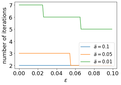
(a) $m(\widehat{a},\epsilon)$.

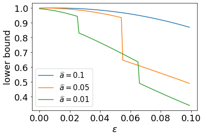
(b) $q(\widehat{a},\epsilon)$.

Figure 1: Effect of $\epsilon$-approximation of $a$ for amplitude amplification. On the left-hand side, we report the number of Grover iterations 31 for boosting the acceptance probability as in Theorem 3.2. On the right-hand side, we display the lower bound 32 on the acceptance probability of Algorithm 3.

Proof.

First, note that 29 guarantees that $\widehat{a}\leq 1$ if $0<\epsilon<1/2$. Still, using 29, we have

$$0<\widehat{a}^{\frac{1}{1-2\epsilon}}\leq a\leq\widehat{a}^{\frac{1}{1+2\epsilon}}\leq 1\quad\text{ with }0<\epsilon<1/2.$$ (33)

By using 26 and the fact that $\asin(\cdot)$ is an increasing function on $[0,1]$, we obtain

$$0<\underbrace{\asin\widehat{a}^{\frac{1}{2-4\epsilon}}}_{\theta_{a,-}}\leq\theta_{a}\leq\underbrace{\asin\widehat{a}^{\frac{1}{2+4\epsilon}}}_{\theta_{a,+}}\leq\pi/2.$$

If $(m+1/2)\theta_{a,+}\leq\pi/4$, we have the following guarantee on the acceptance probability

$$0<\sin^{2}((2m+1)\theta_{a,-})\leq\sin^{2}((2m+1)\theta_{a})\leq\sin^{2}((2m+1)\theta_{a,+})\leq 1,$$

since $\sin^{2}(\cdot)$ is increasing on $[0,\pi/2]$. Thus, if we take $m=m(\widehat{a},\epsilon)=\lfloor\pi/4\theta_{a,+}\rfloor$, we can guarantee that the success probability is larger than $\sin^{2}((2m+1)\theta_{a,-})$. ∎

To complete the picture, we need to have a circuit for the so-called “Grover operator” $Q$.

3.3 A circuit for the Grover operator

We have studied in Section 2.1 a circuit for $\mathcal{C}_{\mathsf{X}}=\mathcal{C}(\mathsf{X}_{:1})\dots\mathcal{C}(\mathsf{X}_{:r})$, from which it is easy to deduce a circuit for its inverse $\mathcal{C}_{\mathsf{X}}^{*}=\mathcal{C}(\mathsf{X}_{:r})\dots\mathcal{C}(\mathsf{X}_{:1})$ by using 5. The only new components of the circuit are $S_{0}$ and $S_{r}$, given respectively in 23 and 24. While $S_{0}$ is standard (see Lemma 3.5), we explain in this section how we use the construction of Section 3.1 to build a circuit for $S_{r}$.

We start by defining a reflection.

Lemma 3.3.

Let $1\leq r<n$ and denote by $\operatorname{\mathrm{bin}}(r)=[r_{0},\dots,r_{k-1}]$ the vector of its decomposition in base $2$. Define the unitary

$$O(r)=\left(\sigma_{x}^{1-r_{0}}\otimes\dots\otimes\sigma_{x}^{1-r_{k-1}}\right)\mathrm{CZ}_{k}\left(\sigma_{x}^{1-r_{0}}\otimes\dots\otimes\sigma_{x}^{1-r_{k-1}}\right),$$

where $\mathrm{CZ}_{k}$ is a multiple controlled-$\sigma_{z}$ gate. For all $s\in\{0,\dots,n\}$, we have

$$O(r)\ket{\operatorname{\mathrm{bin}}(s)}=(-1)^{\delta_{rs}}\ket{\operatorname{\mathrm{bin}}(s)}.$$

Proof.

First, by construction $\sigma_{x}^{1-r_{0}}\otimes\dots\otimes\sigma_{x}^{1-r_{k-1}}\ket{\operatorname{\mathrm{bin}}(r)}=\ket{1}^{\otimes k}$. Second, by definition, $\mathrm{CZ}_{k}\ket{1}^{\otimes k}=-\ket{1}^{\otimes k}$ and $\mathrm{CZ}_{k}$ leaves invariant the orthogonal of $\ket{1}^{\otimes k}$. Thus, $O(r)\ket{\operatorname{\mathrm{bin}}(r)}=-(\sigma_{x}^{1-r_{0}}\otimes\dots\otimes\sigma_{x}^{1-r_{k-1}})\ket{1}^{\otimes k}=-\ket{\operatorname{\mathrm{bin}}(r)}.$ Furthermore, for $s\neq r$, $O(r)\ket{\operatorname{\mathrm{bin}}(s)}=(\sigma_{x}^{1-r_{0}}\otimes\dots\otimes\sigma_{x}^{1-r_{k-1}})\ket{1}^{\otimes k}=\ket{\operatorname{\mathrm{bin}}(r)}.$ This is the desired result. ∎

Lemma 3.4 leverages Lemma 3.3 and the construction of [40] to yield a circuit for $S_{r}$.

Lemma 3.4 (Oracle for Grover’s algorithm).

Let the unitary operator $V$ be as defined in (18). Let also $O(r)$ be as defined in Lemma 3.3 and consider a unit-norm $\ket{\psi}\in(\mathbb{C})^{\otimes n}$. We have

$$V^{*}\left(O(r)\otimes I^{\otimes n}\right)V\left(\ket{0}^{\otimes k}\otimes\ket{\psi}\right)=\ket{0}^{\otimes k}\otimes S_{r}\ket{\psi}.$$

Proof.

By construction, for all unit-norm $\ket{\psi}\in(\mathbb{C})^{\otimes n}$, we have 14, namely $V(\ket{0}^{\otimes k}\otimes\ket{\psi})=\sum_{s=0}^{n}\ket{\operatorname{\mathrm{bin}}(s)}\otimes P_{s}\ket{\psi}.$ By acting now with $O(r)$ on the first $k$ qubits and by using next the definition of $S_{r}$ in (24), we find

$$\left(O(r)\otimes I^{\otimes n}\right)V\left(\ket{0}^{\otimes k}\otimes\ket{\psi}\right) =\sum_{s=0}^{n}\ket{\operatorname{\mathrm{bin}}(s)}\otimes(-1)^{\delta_{rs}}P_{s}\ket{\psi}$$

$$=\sum_{s=0}^{n}\ket{\operatorname{\mathrm{bin}}(s)}\otimes P_{s}S_{r}\ket{\psi}.$$ (34)

At this point, we leverage again 14 but with $\ket{\psi}$ replaced by $S_{r}\ket{\psi}$ this time, i.e.,

$$\ket{0}^{\otimes k}\otimes S_{r}\ket{\psi}=V^{*}\sum_{s=0}^{n}\ket{\operatorname{\mathrm{bin}}(s)}\otimes P_{s}S_{r}\ket{\psi}.$$

Combining the latter identity with 34 yields the desired result. ∎

Next, Lemma 3.5 provides a circuit for implementing $S_{0}$.

Lemma 3.5.

Let $\mathrm{CZ}_{n}$ denote the multiple controlled-$\sigma_{z}$ gate of size $n$. Let

$$S_{0}=\left(\sigma_{x}\otimes\dots\otimes\sigma_{x}\right)\mathrm{CZ}_{n}\left(\sigma_{x}\otimes\dots\otimes\sigma_{x}\right).$$

We have $S_{0}\ket{0}^{\otimes n}=-\ket{0}^{\otimes n},$ and, for all $\ket{\phi}$ orthogonal to $\ket{0}^{\otimes n}$, we have $S_{0}\ket{\phi}=\ket{\phi}.$

Proof.

Again, by definition, $\mathrm{CZ}_{n}\ket{1}^{\otimes n}=-\ket{1}^{\otimes n}$ and $\mathrm{CZ}_{n}$ leaves invariant the orthogonal of $\ket{1}^{\otimes n}$. ∎

By composing the building blocks in Lemma 3.4 and Lemma 3.5, we have a circuit for Grover’s operator.

Theorem 3.6 (A circuit for Grover’s operator).

In the setting of Section 3.2, let $Q$ be given in 22. Define

$$C=-(I^{\otimes k}\otimes\mathcal{C}_{\mathsf{X}})(I^{\otimes k}\otimes S_{0})(I^{\otimes k}\otimes\mathcal{C}_{\mathsf{X}}^{*})V^{*}\left(O(r)\otimes I^{\otimes n}\right)V$$

where $S_{0}$ is given in Lemma 3.5 and $O(r)$ is defined in Lemma 3.3. We have

$$C(\ket{0}^{\otimes k}\otimes\ket{\psi})=\ket{0}^{\otimes k}\otimes Q\ket{\psi}.$$

Proof.

Using Lemma 3.4, we have

$$-C(\ket{0}^{\otimes k}\otimes\ket{\psi}) =(I^{\otimes k}\otimes\mathcal{C}_{\mathsf{X}})(I^{\otimes k}\otimes S_{0})(I^{\otimes k}\otimes\mathcal{C}_{\mathsf{X}}^{*})\left(\ket{0}^{\otimes k}\otimes S_{r}\ket{\psi}\right)$$

$$=\ket{0}^{\otimes k}\otimes\mathcal{C}_{\mathsf{X}}S_{0}\mathcal{C}_{\mathsf{X}}^{*}S_{r}\ket{\psi},$$

which concludes the proof. ∎

This concludes the presentation of our fast quantum sampler for projection DPPs. Before turning to experimental validation, we now examine the point process that results from measuring the occupation number without applying any rejection step.

4 A DPP with nonsymmetric correlation kernel

To better describe the point process associated with 10, we first need to introduce useful notations. Denote the upper triangular part of a square matrix $A$ by $\mathrm{triu}(A)$. Let $\mathsf{X}\in\mathbb{R}^{n\times r}$ be a matrix with unit-norm columns. Now, define the skewsymmetric matrix $\mathrm{skew}(A)=\mathrm{triu}(A)-\mathrm{triu}(A)^{\top}$. For instance, by taking a matrix $\mathsf{X}=[\mathsf{X}_{:1}\ \mathsf{X}_{:2}\ \mathsf{X}_{3:}]$ with columns of unit norm, it comes

$$\mathrm{skew}\left(\mathsf{X}^{\top}\mathsf{X}\right)=\begin{bmatrix}0&\mathsf{X}_{:1}^{\top}\mathsf{X}_{:2}&\mathsf{X}_{:1}^{\top}\mathsf{X}_{:3}\\ -\mathsf{X}_{:1}^{\top}\mathsf{X}_{:2}&0&\mathsf{X}_{:2}^{\top}\mathsf{X}_{:3}\\ -\mathsf{X}_{:1}^{\top}\mathsf{X}_{:3}&-\mathsf{X}_{:2}^{\top}\mathsf{X}_{:3}&0\end{bmatrix}.$$

4.1 Definition and properties

Consider again the state $\ket{\mathrm{columns}(\mathsf{X})}=\mathcal{C}(\mathsf{X}_{:1})\dots\mathcal{C}(\mathsf{X}_{:r})\ket{\emptyset}$ as given in 6. Let $Y$ be the point process associated with the measure of the occupation numbers

$$[N_{1},\dots,N_{n}]\text{ with }N_{i}\triangleq c_{i}^{*}c_{i}\text{ for }i\in\{1,\dots n\},$$

in the state $\ket{\mathrm{columns}(\mathsf{X})}$; as given by 10. Hence, $[N_{1},\dots,N_{n}]$ is associated with a random vector in $\{0,1\}^{n}$.

Theorem 4.1 (DPP associated with a Clifford loader).

Let $\mathsf{X}\in\mathbb{R}^{n\times r}$ be a matrix with unit-norm columns such that $\rank(\mathsf{X})=r$. The point process $Y$ defined in 10 and associated with the measure of the occupation numbers $N_{1},\dots,N_{n}$ in the state $\ket{\mathrm{columns}(\mathsf{X})}$ given in (8) has the following law

$$\mathbb{P}(Y=\mathtt{C})=\det\begin{bmatrix}0_{|\mathtt{C}|}&\mathsf{X}_{\mathtt{C}:}\\ -(\mathsf{X}_{:\mathtt{C}})^{\top}&\mathrm{skew}(\mathsf{X}^{\top}\mathsf{X})\end{bmatrix},$$

where $\mathtt{C}\subseteq\{1,\dots,n\}$. In particular, we have $\mathbb{P}(\mathrm{parity}(|Y|)\neq\mathrm{parity}(r))=0.$

Before giving a proof, we first emphasize that it is manifest that $\mathbb{P}(Y=\mathtt{C})\geq 0$ since it is the determinant of a skewsymmetric matrix. It is however less obvious that $\mathbb{P}(Y=\mathtt{C})\leq 1$. We show this fact in the following proof, by proving that $\sum_{\mathtt{C}}\mathbb{P}(Y=\mathtt{C})=1$. Second, there is no reason for the above DPP to be invariant if the columns of $\mathsf{X}$ are permuted. In Remark 5.2 in the sequel, we discuss an example in which different orderings of the columns of $\mathsf{X}$ yield different DPP laws.

Proof.

Consider the definition of $\ket{\mathrm{columns}(\mathsf{X})}$ in (8). A simple argument based on Wick’s theorem (see Section B.1 for more details) gives

$$\ket{\mathrm{columns}(\mathsf{X})}=\sum_{\begin{subarray}{c}0\leq\ell\leq r:\\ \text{parity}(r)=\text{parity}(\ell)\end{subarray}}\sum_{\begin{subarray}{c}\mathtt{S}:|\mathtt{S}|=\ell\\ \text{ordered}\end{subarray}}\mathrm{pf}\begin{bmatrix}0_{\ell}&\mathsf{X}_{\mathtt{S}:}\\ -(\mathsf{X}^{\top})_{:\mathtt{S}}&\mathrm{skew}(\mathsf{X}^{\top}\mathsf{X})\end{bmatrix}\prod_{i\in\mathrm{rev}(\mathtt{S})}c_{i}^{*}\ket{\emptyset},$$ (35)

where $\mathsf{X}_{\mathtt{S}:}\in\mathbb{R}^{\ell\times r}$ is by construction such that $\ell+r$ is even. Note that, in the formula above, we take the convention that

$$\begin{bmatrix}&\mathsf{X}_{\emptyset:}\\ -(\mathsf{X}^{\top})_{:\emptyset}&\mathrm{skew}(\mathsf{X}^{\top}\mathsf{X})\end{bmatrix}\triangleq\mathrm{skew}(\mathsf{X}^{\top}\mathsf{X}).$$

To gain intuition, here is an example with $r=3$. Let $i\in\{1,2,3\}$. The amplitude in front of $c_{i}^{*}\ket{\emptyset}$ (corresponding to $\mathtt{S}=(i)$) reads

$$\mathrm{pf}\begin{bmatrix}0&\mathsf{X}_{i1}&\mathsf{X}_{i2}&\mathsf{X}_{i3}\\ &0&\mathsf{X}_{:1}^{\top}\mathsf{X}_{:2}&\mathsf{X}_{:1}^{\top}\mathsf{X}_{:3}\\ &&0&\mathsf{X}_{:2}^{\top}\mathsf{X}_{:3}\\ &&&0\end{bmatrix}=\mathsf{X}_{i1}(\mathsf{X}_{:2}^{\top}\mathsf{X}_{:3})-\mathsf{X}_{i2}(\mathsf{X}_{:1}^{\top}\mathsf{X}_{:3})+\mathsf{X}_{i3}(\mathsf{X}_{:1}^{\top}\mathsf{X}_{:2}).$$

We have – as a particular case – for any ordered subset such that $|\mathtt{S}|=r$,

$$\mathrm{pf}\begin{bmatrix}0_{r}&\mathsf{X}_{\mathtt{S}:}\\ -(\mathsf{X}^{\top})_{:\mathtt{S}}&\mathrm{skew}(\mathsf{X}^{\top}\mathsf{X})\end{bmatrix}=(-1)^{r(r-1)/2}\det(\mathsf{X}_{\mathtt{S}:}),$$

as a consequence of Lemma B.2, given in appendix, so that we recover the second term in 7. Now let $\mathtt{C}$ be a subset of $\{1,\dots,n\}$ with $|\mathtt{C}|\leq r$. Coming back to the expression of $\ket{\mathrm{columns}(\mathsf{X})}$, the probability $\mathbb{P}(Y=\mathtt{C})$ is given by the squared modulus of the coefficient of $\prod_{i\in\mathtt{C}}c_{i}^{*}\ket{\emptyset}$ in 35 as a consequence of 10 (Born’s rule), i.e.,

$$\mathbb{P}(Y=\mathtt{C})=\left|\mathrm{pf}\begin{bmatrix}0_{\ell}&\mathsf{X}_{\mathtt{C}:}\\ -(\mathsf{X}^{\top})_{:\mathtt{C}}&\mathrm{skew}(\mathsf{X}^{\top}\mathsf{X})\end{bmatrix}\right|^{2}=\det\begin{bmatrix}0_{\ell}&\mathsf{X}_{\mathtt{C}:}\\ -(\mathsf{X}^{\top})_{:\mathtt{C}}&\mathrm{skew}(\mathsf{X}^{\top}\mathsf{X})\end{bmatrix},$$

since all matrices have real entries here. Note that this is a well-normalized probability mass function. Let us briefly explain why. First, the matrix

$$\begin{bmatrix}0_{\ell}&\mathsf{X}_{\mathtt{C}:}\\ -(\mathsf{X}^{\top})_{:\mathtt{C}}&\mathrm{skew}(\mathsf{X}^{\top}\mathsf{X})\end{bmatrix}$$

is skewsymmetric with an even number of rows and columns. Hence, its determinant cannot be negative. Second, we show that $\mathbb{P}(Y=\mathtt{C})$ sums up to unity. Let us use the following identity [32, Theorem 2.1]

$$\sum_{\begin{subarray}{c}\mathtt{C}^{\prime}\subseteq\{1,\dots,n^{\prime}\}\\ \mathtt{A}^{\prime}\subseteq\mathtt{C}^{\prime}\end{subarray}}\det L_{\mathtt{C}^{\prime}\mathtt{C}^{\prime}}=\det(L+1_{\overline{\mathtt{A}^{\prime}}}),$$ (36)

by choosing $n^{\prime}=r+n$. Here, we introduced the diagonal matrix $[1_{{\mathtt{C}}}]_{i,j}=\delta_{ij}1(i\in\mathtt{C})$ whose diagonal contains the indicator vector of $\mathtt{C}$. Upon denoting

$$L=\begin{bmatrix}0_{n}&\mathsf{X}\\ -\mathsf{X}^{\top}&\mathrm{skew}(\mathsf{X}^{\top}\mathsf{X})\end{bmatrix},$$ (37)

we have that

$$\sum_{\begin{subarray}{c}\mathtt{C}^{\prime}\subseteq\{1,\dots,r+n\}\\ n+\{1,\dots,r\}\subseteq\mathtt{C}^{\prime}\end{subarray}}\det L_{\mathtt{C}^{\prime}\mathtt{C}^{\prime}}=\det(L+1_{\overline{n+\{1,\dots,r\}}})=\det\begin{bmatrix}I_{n}&\mathsf{X}\\ -\mathsf{X}^{\top}&\mathrm{skew}(\mathsf{X}^{\top}\mathsf{X})\end{bmatrix}.$$

By using the formula for the determinant of block matrices, we find

$$\det\begin{bmatrix}I_{n}&\mathsf{X}\\ -\mathsf{X}^{\top}&\mathrm{skew}(\mathsf{X}^{\top}\mathsf{X})\end{bmatrix}=\det(\mathrm{skew}(\mathsf{X}^{\top}\mathsf{X})+\mathsf{X}^{\top}\mathsf{X}).$$

Since $\mathrm{skew}(\mathsf{X}^{\top}\mathsf{X})+\mathsf{X}^{\top}\mathsf{X}$ is triangular with only ones on its diagonal, its determinant is equal to $1$. This completes the proof. ∎

Actually, the proof of Theorem 4.1 inspires the following generalization.

Theorem 4.2.

Let $X\in\mathbb{R}^{n\times r}$ be a matrix with linearly independent columns and let $A\in\mathbb{R}^{r\times r}$ be skewsymmetric. The determinantal point process with law

$$\mathbb{P}(Y=\mathtt{C})=\frac{1}{\det(A+X^{\top}X)}\det\begin{bmatrix}0_{|\mathtt{C}|}&X_{\mathtt{C}:}\\ -(X_{\mathtt{C}:})^{\top}&A\end{bmatrix}\text{ with }\mathtt{C}\subseteq\{1,\dots,n\}$$

is well-defined.

Proof.

Note that $\det(A+X^{\top}X)=\det(X^{\top}X)\det(S+I_{r})$ where

$$S=(X^{\top}X)^{-1/2}A(X^{\top}X)^{-1/2}$$

is skewsymmetric. Thus, $\det(A+X^{\top}X)>0$. Hence, $\mathbb{P}(Y=\mathtt{C})\geq 0$. That it is the correct normalization factor follows from the arguments in the proof of Theorem 4.1. ∎

Note that similar DPPs – called $L$-ensembles – were described in [20, 21] which consider the case of a skewsymmetric matrix $L$ as in 38. Incidentally, the DPP in Theorem 4.2 involves only specific principal minors of the matrix $L$ in 38, namely the ones which always include the last $r$ rows and columns. In light of this remark, this type of DPPs is a skewsymmetric analogue of the so-called extended $L$-ensembles of [45], where the authors only consider Hermitian matrices $L$. For completeness, we give the correlation kernel of the DPP defined in Theorem 4.2 in Corollary 4.3, which has a particularly intuitive form since it is a deformation of the orthogonal projector 2.

Corollary 4.3.

Let $Y$ be the point process of Theorem 4.2. We have

$$\mathbb{P}(\mathtt{A}\subseteq Y)=\det(X(A+X^{\top}X)^{-1}X^{\top})_{\mathtt{A}\mathtt{A}}.$$

Proof.

Let us again use the identity 36 by choosing $n^{\prime}=r+n$ and $L$ to be the $(n+r)\times(n+r)$ matrix given by

$$L=\begin{bmatrix}0_{n}&X\\ -X^{\top}&A\end{bmatrix},$$ (38)

and $\mathtt{A}^{\prime}=r+\mathtt{A}$ with $\mathtt{A}\subseteq\{1,\dots,n\}$. At this point, we can compute

$$\det(L+1_{\overline{n+\{1,\dots,r\}}})=\det(A+X^{\top}X)=1,$$

where we used the notation $[1_{{\mathtt{C}}}]_{i,j}=\delta_{ij}1(i\in\mathtt{C})$. Hence, $L+1_{\overline{n+\{1,\dots,r\}}}$ is invertible. Thus, we find

$$\mathbb{P}(\mathtt{A}\subseteq Y) =\sum_{\mathtt{C}:\mathtt{A}\subseteq\mathtt{C}}\mathbb{P}(Y=\mathtt{C})$$

$$=\det(L+1_{\overline{\mathtt{A}^{\prime}}})$$

$$=\det(L+1_{\overline{n+\{1,\dots,r\}}})\det\left(L\left(L+1_{\overline{n+\{1,\dots,r\}}}\right)^{-1}\right)_{\mathtt{A}^{\prime}\mathtt{A}^{\prime}}.$$ (39)

To obtain the last equality, we used identities from [32, proof of Theorem 2]. The result follows from the use of the well-known formula for the inverse of a block matrix. ∎

Next, we give in Lemma 4.4 an expression of the spectral decomposition of the correlation kernel which is later used to derive the law of the number of points sampled by the process.

Lemma 4.4 (Spectral decomposition).

Under the hypotheses of Theorem 4.2, let $K=X(A+X^{\top}X)^{-1}X^{\top}$ and define the $r\times r$ matrix $S=(X^{\top}X)^{-1/2}A(X^{\top}X)^{-1/2}$. On the one side, if $r=2k+1$ for some $k\geq 1$, we have

$$K=V\left(v_{0}v_{0}^{\top}+\sum_{\ell=1}^{k}\frac{1-\mathrm{i}\nu_{\ell}}{1+\nu_{\ell}^{2}}u_{\ell}u_{\ell}^{*}+\frac{1+\mathrm{i}\nu_{\ell}}{1+\nu_{\ell}^{2}}\bar{u}_{\ell}\bar{u}_{\ell}^{*}\right)V^{\top},$$ (40)

where $V=X(X^{\top}X)^{-1/2}$ has orthonormal columns. In 40, we used the Youla decomposition of $S$, namely the normalized eigenpairs $(i\nu_{\ell},u_{\ell})$ and $(-i\nu_{\ell},\bar{u}_{\ell})$ with $\nu_{\ell}$ real for all $\ell\in\{1,\dots,k\}$, whereas $v_{0}$ is the unpaired eigenvector of $S$ of zero eigenvalue. Also, we have the decomposition of the unit vectors $u_{\ell}=(a_{\ell}+\mathrm{i}b_{\ell})/\sqrt{2}$ where $(a_{\ell},b_{\ell})_{\ell}$ are mutually orthogonal real unit vectors. On the other side, if $r=2k$ for some $k\geq 1$, the same decomposition holds in the absence of $v_{0}$.

Proof.

The result follows from writing

$$K=X(X^{\top}X)^{-1/2}(S+I_{r})^{-1}(X^{\top}X)^{-1/2}X^{\top},$$

and by using the Youla decomposition of the real skewsymmetric matrix $S$. ∎

Before going further, let us understand the expression in 40. Considering one term on the right-hand side for simplicity, we can write the paired eigenvectors in terms of a real part and an imaginary part as follows $u=(a+\mathrm{i}b)/\sqrt{2}$ and $\bar{u}=(a-\mathrm{i}b)/\sqrt{2}$. Further, denote $\alpha=1/(1+\nu^{2})$ and $\beta=\nu/(1+\nu^{2})$, which are such that that $0<\alpha\leq 1$ and $0\leq|\beta|\leq 1$. Hence, we have

$$\begin{bmatrix}u&\bar{u}\end{bmatrix}\begin{bmatrix}\alpha-\mathrm{i}\beta&0\\ 0&\alpha+\mathrm{i}\beta\end{bmatrix}\begin{bmatrix}u^{*}\\ \bar{u}^{*}\end{bmatrix}=\begin{bmatrix}a&b\end{bmatrix}\begin{bmatrix}\alpha&\beta\\ -\beta&\alpha\end{bmatrix}\begin{bmatrix}a^{\top}\\ b^{\top}\end{bmatrix}=\alpha(aa^{\top}+bb^{\top})+\beta(ab^{\top}-ba^{\top}),$$

where we actually see the role played by $\beta$ in the skewsymmetric part of the matrix.

We are now ready to describe the law of the number of points of the process.

Proposition 4.5 (Law of cardinal of a sample).

In the setting of Lemma 4.4, let $Y\sim\mathrm{DPP}(K)$ where $K=X(A+X^{\top}X)^{-1}X^{\top}$ is $n\times n$ and with an $r\times r$ skewsymmetric matrix $A$. If $r=2k+1$, the law of the number of points in a sample of $Y$ is

$$|Y|=1+2\sum_{\ell=1}^{k}\text{Bern}\left(\frac{1}{1+\nu_{\ell}^{2}}\right)$$

where the Bernoulli random variables are independent. Otherwise, if $r=2k$, the law of $|Y|$ is the same as above with the constant “$1$” removed.

Proof.

Classically, the law of the cardinal of $Y$ is expressed as a determinant [13, Corollary 1 in Supplemantary Material], namely

$$\mathbb{E}[z^{|Y|}]=\det(I_{n}-K+zK).$$

Consider the case of odd $r$. Denoting $\mu_{\ell}=\frac{1-\mathrm{i}\nu_{\ell}}{1+\nu_{\ell}^{2}}$, the spectral decomposition in Lemma 4.4 yields

$$\mathbb{E}[z^{|Y|}]=z\prod_{\ell=1}^{k}(1-\mu_{\ell}+z\mu_{\ell})(1-\bar{\mu}_{\ell}+z\bar{\mu}_{\ell})=z\prod_{\ell=1}^{k}\left(\frac{\nu_{\ell}^{2}}{1+\nu_{\ell}^{2}}+\frac{z^{2}}{1+\nu_{\ell}^{2}}\right),$$

where we observe that the above product involves moment generating functions of Bernoullis with success probability $1/(1+\nu_{\ell}^{2})$. The case of even $r$ follows from the same reasoning. ∎

4.2 Example: sampling uniform spanning trees

In this section, we particularize the DPP of Theorem 4.1 to highlight its connections with a well-known DPP on graph edges. A spanning tree of a graph is a connected subgraph with the same vertex set and edges forming no cycle. The edges of a spanning tree sampled uniformly are known to be a projection DPP [38]. The point process of Theorem 4.1 is in fact a generalization of this DPP.

We begin by setting a few definitions. Let $B$ denote the edge-vertex incidence matrix of an unweighted finite and connected graph. The Laplacian of this graph is customarily defined as $L=B^{\top}B$. For further use, denote by $\mathrm{deg}(i)$ the number of neighbors of node $i$ and let $D$ be the diagonal matrix with entry $ii$ being $\mathrm{deg}(i)$. To sample spanning trees with the algorithm of Section 2.4, one needs to first choose a node $\varrho$, called the root. Then, we define the matrix $X=B_{:\widehat{\varrho}}$ obtained from $B$ by removing the column of the root node. Note that $\|X_{:,i}\|^{2}_{2}=\mathrm{deg}(i)$ for all nodes $i\neq\varrho$. Thus, define the column-normalized incidence matrix $\mathsf{B}=BD^{-1/2}$.

4.2.1 Probability distribution over dimer-rooted forests

As can be seen by a direct substitution, the DPP associated with $\ket{\mathrm{columns}(\mathsf{X})}$ is in fact a measure over edges of dimer-rooted forests which are defined in Definition 4.6. We refer to Figure 5 for an illustration.

Definition 4.6 (dimer-rooted forest with root $\varrho$).

Let $G$ be a finite connected graph with $n_{v}$ nodes and let $\varrho$ be one of its nodes. A dimer-rooted forest of $G$ with root $\varrho$ is a set of edges $\mathtt{C}$ which satisfies the following conditions:

• $\mathtt{C}$ contains no cycle and is such that $\text{parity}(\mathtt{C})=\text{parity}(n_{v}-1)$,

• $\mathtt{C}$ can be completed to a spanning subgraph by complementing it by an edge-disjoint set of dimers such that the connected components of $\mathtt{C}$ are either trees rooted to $\varrho$ or trees rooted to one dimer.

Note that the dimers are not part of the dimer-rooted forest. These dimer-rooted forests are closely related to dimer covers, namely sets of edges such that each node is the endpoint of exactly one edge. In a word, each dimer in the dimer-rooted forests corresponds to a contraction in the expansion of a Pfaffian as detailed in Appendix B. This is illustrated from the graph viewpoint in Figure 2 where the colored edges indicate the superposition of edges coming with the neighbourhood of each colored node.

Figure 2: A simple square graph and the corresponding Clifford loader $\mathcal{C}(\mathsf{B}_{:1})\mathcal{C}(\mathsf{B}_{:2})\mathcal{C}(\mathsf{B}_{:4})\ket{\emptyset}$; see 8. We here defined the normalized incidence matrix $\mathsf{B}=BD^{-1/2}$ and the notation $f_{e}=c_{e}+c_{e}^{*}$ for any edge $e$. The column $\varrho=3$ is removed from $\mathsf{B}$. The colored edges emanate from the node of the same color whereas their orientation is determined (by convention) by the matrix $B$.

Indeed, in the decomposition of $\ket{\text{columns}(\mathsf{B}_{:\widehat{\varrho}})}$, the origin of the dimers is the annihilation (or contraction, i.e., $(c_{e}+c_{e}^{*})^{2}=\mathbb{I}$) of identical edges coming from neighbouring nodes.

Theorem 4.7 (determinantal measure over dimer-rooted forests).

Consider a connected graph with $n_{v}$ nodes and $n_{e}$ edges. Denote by $B$ its $n_{e}\times n_{v}$ incidence matrix. Let $\varrho\in\{1,\dots,n_{v}\}$ be any node of this graph. Let $Y$ be a DPP with law

$$\mathbb{P}(Y=\mathtt{C})=\left(\prod_{\begin{subarray}{c}i=1\\ i\neq\varrho\end{subarray}}^{n_{v}}\mathrm{deg}(i)\right)^{-1}\cdot\det\begin{bmatrix}0_{|\mathtt{C}|}&B_{\mathtt{C}\widehat{\varrho}}\\ -(B_{\mathtt{C}\widehat{\varrho}})^{\top}&\mathrm{skew}(L_{\widehat{\varrho}\widehat{\varrho}})\end{bmatrix}\text{ with }\mathtt{C}\subseteq\{1,\dots,n_{e}\}.$$

If $\mathbb{P}(Y=\mathtt{C})\neq 0$, then $\mathtt{C}$ is necessarily the set of simple edges of a dimer-rooted forest; see Definition 4.6.

Proof.

Define for convenience

$${A}\triangleq\begin{bmatrix}0_{|\mathtt{C}|}&B_{\mathtt{C}\widehat{\varrho}}\\ -(B_{\mathtt{C}\widehat{\varrho}})^{\top}&\mathrm{skew}(L_{\widehat{\varrho}\widehat{\varrho}})\end{bmatrix}.$$ (41)

First, we observe that if $\mathtt{C}$ includes edges forming a cycle, then the corresponding rows of the first block of 41, i.e. $\begin{bmatrix}0_{|\mathtt{C}|}&B_{\mathtt{C}\widehat{\varrho}}\\ \end{bmatrix}$, are linearly dependent, since the corresponding rows of $B_{\mathtt{C}\widehat{\varrho}}$ are linealy dependent. Therefore, $\mathtt{C}$ cannot include any cycle otherwise $\det A=0$. Similarly, $\text{parity}(\mathtt{C})=\text{parity}(n_{v}-1)$, since otherwise $A$ has an odd number of rows and columns and therefore, $\det A=0$. We thus see that $(i)$ in Definition 4.6 is necessary, and in what follows, we assume $\text{parity}(\mathtt{C})=\text{parity}(n_{v}-1)$.

Second, note that $C=\mathrm{skew}(L_{\widehat{\varrho}\widehat{\varrho}})$ can be interpreted as a skewsymmetric adjacency matrix where each edge is endowed with an orientation as follows:

$${C}_{ij}=\begin{cases}+1&\text{ if }ij\text{ is an oriented edge},\\ -1&\text{ if }ji\text{ is an oriented edge},\\ 0&\text{ otherwise.}\end{cases}$$

Recall that we denote edges by pairs $(i,j)$ with $i<j$; see Figure 3 for an illustration.

Figure 3: Orientation associated to the matrix $\mathrm{skew}(L_{\widehat{\varrho}\widehat{\varrho}})$ for a simple graph. Edge orientations are determined by the ordering of the nodes. Dashed edges are missing after removing $\varrho$.

Hence, by examining 41, we realize that the matrix ${A}$ can be interpreted as a skewsymmetric adjacency matrix of an augmented graph where the edges in $\mathtt{C}$ are considered as additional vertices, namely whose vertex set is

$$\mathcal{V}=\mathtt{C}\cup\{1,\dots,\widehat{\varrho},\dots,n_{v}\},$$

where $\dots,\widehat{\varrho},\dots$ indicates that the vertex $\varrho$ is missing. Above, each edge $ij$ in $\mathtt{C}$ is considered as an extra node of the augmented graph which is only connected to its neighbours $i$ and $j$; see Figure 4 for an illustration. Now, we recall that $\det A=(\mathrm{pf}{A})^{2}$ since ${A}$ is skewsymmetric with an even number of rows as a consequence of $(i)$. By using the definition of the Pfaffian as a sum over contractions (see Section B.1 for the exact expression), we see that, if $\mathrm{pf}{A}\neq 0$, there should exist at least one permutation $\sigma$ such that ${A}_{\sigma(1)\sigma(2)}\dots A_{\sigma(2k-1)\sigma(2k)}\neq 0,$ with $2k=|\mathtt{C}|+(n_{v}-1)$. Hence, this permutation determines a dimer cover of the augmented graph. Thus, coming back to the expression 41, $\det A\neq 0$ implies that there exists a dimer configuration of the augmented graph, which by definition should visit all the nodes of the augmented graph, and hence should include a pair $(e,v_{e})$ for all $e\in\mathtt{C}$ where $v_{e}$ is an endpoint of $e$. This yields to condition $(ii)$ in Definition 4.6. Thus, the conditions $(i)$ and $(ii)$ are necessary.

∎

Figure 4: An augmented graph covered by a dimer configuration (thick edges). Here, the edges in $\mathtt{C}=\{(1,2),(2,3),(3,\varrho),(11,\varrho),(10,9)\}$ are depicted as teal rectangles whereas the perfect matching spanning the remaining nodes is colored in blue. The nodes of the original graph are displayed as circles.

Figure 5: A dimer-rooted forest with root $\varrho$ and whose edges – colored in teal – are $\mathtt{C}=\{(1,2),(2,3),(3,\varrho),(11,\varrho),(10,9)\}$. This dimer-rooted forest is associated with the augmented graph of Figure 4.

Considering a connected graph with no self-loop, let $D=\mathrm{Diag}(\mathrm{deg})$ denote the diagonal degree matrix. It is customary to define the normalized Laplacian as

$$L^{(N)}=D^{-1/2}LD^{-1/2}.$$ (42)

Key properties of $L^{(N)}$ are that its diagonal contains only ones and that it is positive semi-definite. Let $L^{(N)}_{\widehat{\varrho}\widehat{\varrho}}$ be the normalized Laplacian with the row and column associated with the root $\varrho$ removed, which is non-singular. By Hadamard’s inequality, $\det L^{(N)}_{\widehat{\varrho}\widehat{\varrho}}\leq 1$. The acceptance probability of the algorithm of Section 2.4 reads

$$a\triangleq\det L^{(N)}_{\widehat{\varrho}\widehat{\varrho}}=\frac{\det L_{\widehat{\varrho}\widehat{\varrho}}}{\prod_{i\neq\varrho}\mathrm{deg}(i)}=\frac{\sharp\text{STs}}{\prod_{i\neq\varrho}\mathrm{deg}(i)},$$ (43)

where $\sharp\text{STs}$ denotes the number of spanning trees of the graph. This expression shows that, for a given graph, we can maximize the acceptance probability in Algorithm 1 by choosing a node $\varrho$ with maximum degree. To fix ideas, we now list two examples of graphs which exhibit different typical decays for $a$.

Example 4.8 (Complete graph).

For the complete graph of $n$ nodes with $n\geq 2$, $\sharp\text{STs}=n^{n-2}$; see e.g., Figure 9(a) for an illustration. Thus, in this case, the acceptance probability reads

$$a=n^{-1}\left(\frac{n}{n-1}\right)^{n-1}=\Theta(n^{-1}),\text{ for any root node }\varrho.$$

It is easy to see that it satisfies $2/n\leq a\leq e/n$ where $e$ is Euler’s constant.

Example 4.9 (Barbell graph).

Consider a barbell graph of $n$ nodes with two complete graphs of $n^{\prime}$ nodes connected by a line graph of $n^{\prime\prime}$ nodes; see e.g., Figure 9(b) for an illustration with $n^{\prime}=3$ and $n^{\prime\prime}=0$. In that case, by noting that $\sharp\text{STs}=n^{\prime 2{n}^{\prime}-4}$ for $n^{\prime}\geq 2$, we find that the acceptance probability reads

$$a=\mathrm{deg}(\varrho)\left(\frac{n^{\prime}}{n^{\prime}-1}\right)^{2n^{\prime}-2}n^{\prime-4}2^{-n^{\prime\prime}},\text{ with $\varrho$ the root node}.$$

Also, we have $4n^{\prime-4}2^{-n^{\prime\prime}}\leq a/\mathrm{deg}(\varrho)\leq e^{2}n^{\prime-4}2^{-n^{\prime\prime}}$. In order to maximize the acceptance probability, we choose $\varrho$ as a connecting node between a clique and the line graph. Then, we have $a=\Theta(n^{\prime-3}2^{-n^{\prime\prime}})$ where we can take for example $n^{\prime}=n^{\prime\prime}=n/3$.

Thus, the decay of the acceptance probability in Example 4.9 is very fast as the graph grows in size. In Section 3, we propose a circuit to boost this probability. Before reaching this section, we compare the determinantal formula 43 for $a$ to similar quantities appearing in rejection sampling (RS). We indeed show in Section 4.2.2 that $a$ is the acceptance probability of a closely related classical RS algorithm.

4.2.2 Acceptance probability for vanilla rejection sampling

Interestingly, the expression of the acceptance probability 43 – the inverse number of rejections before acceptance – can be compared to a similar quantity appearing in a famous classical algorithm for sampling uniform spanning trees, i.e., Wilson’s cycle-popping algorithm [48]. This algorithm which has both a random walk formulation or a stacks-of-cards formulation is discussed more generally in the partial rejection sampling framework (PRS) in [26] and [22]. First, by using the expression 42, we rewrite the acceptance probability in Algorithm 1 as follows

$$a=\det(I_{n-1}-\Pi_{\widehat{\varrho}\widehat{\varrho}}),$$ (44)

where $\Pi$ is the transition matrix of the customary random walk with uniform jumps to neighbours, namely, $\Pi_{ij}=1/\mathrm{deg}(i)$ if $j\sim i$ and $\Pi_{ij}=0$ otherwise. At this point, we connect the expression of $a$ to the stacks-of-cards description of Wilson’s cycle-popping algorithm.

Consider a random variable $U_{i}$ per node $i\neq\varrho$ which yields a neighbour of $i$ – say $j$ – with probability $\Pi_{ij}$. Each $U_{i}$ is visualized as a card positioned over node $i$, and its value is interpreted as an edge between $i$ and a neighbour $U_{i}$. We assume that all these variables are mutually independent. By inspection, a realization of $U_{1},\dots,\widehat{U_{\varrho}},\dots,U_{n}$ yields an oriented spanning subgraph which may contain cycles. By cycles, we mean oriented cycles including backtracks (2-cycles). Denote this oriented spanning subgraph by $\mathrm{subgraph}(U_{1},\dots,\widehat{U_{\varrho}},\dots,U_{n})$. The stacks-of-cards algorithm goes as follows. First, fix an order of the cycles.

• Sample $U_{1},\dots,\widehat{U_{\varrho}},\dots,U_{n}$ independently.

• While $\mathrm{subgraph}(U_{1},\dots,\widehat{U_{\varrho}},\dots,U_{n})$ contains cycles, resample (or pop) all the $U_{i}$’s which are part of the smallest cycle in the order. Otherwise, stop and output the spanning tree given by the $U_{i}$’s.

Note that this algorithm finishes with probability one and that it outputs a uniform spanning tree as well as the history of erased cycles. These ‘popped’ cycles can be organized as a heap of cycles, i.e., a combinatorial structure defined by [47]; see Section 5.7.2 of [19] for a pedestrian exposition. Following [26], the expression 44 equals

$$a=\Pr_{\prod_{i\neq\varrho}U_{i}}[\mathrm{subgraph}(U_{1},\dots,\widehat{U_{\varrho}},\dots,U_{n})\text{ contains no cycle}],$$ (45)

or, in other words, $a$ is the probability that – if $U_{1},\dots,\widehat{U_{\varrho}},\dots,U_{n}$ are sampled independently – $\mathrm{subgraph}(U_{1},\dots,\widehat{U_{\varrho}},\dots,U_{n})$ is a spanning tree.

Thus, we see that 45 is exactly the inverse expected number of rejections before acceptance if the edges are sampled following $\prod_{i\neq\varrho}U_{i}$. This is the classical case of vanilla RS. In contrast, according to [26, Corollary 7], the expected number of iteration before acceptance in the partial rejection sampling (PRS) framework (Wilson’s algorithm) reads

$$\frac{\Pr_{\prod_{i\neq\varrho}U_{i}}[\mathrm{subgraph}(U_{1},\dots,\widehat{U_{\varrho}},\dots,U_{n})\text{ contains exactly one cycle}]}{\Pr_{\prod_{i\neq\varrho}U_{i}}[\mathrm{subgraph}(U_{1},\dots,\widehat{U_{\varrho}},\dots,U_{n})\text{ contains no cycle}]},$$

which can be much smaller compared with $1/a$ (vanilla RS 45) since the numerator can be much smaller than $1$.

4.2.3 Sketching acceptance probability in the graph case

We discuss here the choice of parameter $\theta_{1}$ for the sketching algorithm of [9] and the associated complexity 3. The basic idea is that the complexity of the sketch is low provided that the graph has a good connectivity. Recall that we choose $\mathsf{X}=\mathsf{B}_{:\widehat{\varrho}}\in\mathbb{R}^{n\times r}$ where $\mathsf{B}=BD^{-1/2}$ is the column-normalized incidence matrix of a connected graph with $n$ edges and $n_{v}=r+1$ nodes.

A connected graph with a hub node.

To bound the spectrum of $\mathsf{X}^{\top}\mathsf{X}=L^{(N)}_{\widehat{\varrho}\widehat{\varrho}}$ from below, we begin by proving the following lemma, inspired from [23, Section 3.3].

Lemma 4.10.

Consider a connected graph with no self-loop and let $L=B^{\top}B$ be its combinatorial Laplacian. If there exists a node $\varrho$ connected to all the other nodes, we have $\lambda_{\min}(L_{\widehat{\varrho}\widehat{\varrho}})\geq 1$.

Proof.

We use the Gershgorin circle theorem: $\lambda_{\min}(L_{\widehat{\varrho}\widehat{\varrho}})$ is at least in one closed disc $i_{\star}$ of center $\mathrm{deg}(i_{\star})$ and radius $\sum_{j\neq i_{\star},j\neq\varrho}1(i_{\star}\sim j)$. Since the graph is connected, the latter quantity reads $\mathrm{deg}(i_{\star})-1$. Thus, $\lambda_{\min}(L_{\widehat{\varrho}\widehat{\varrho}})\geq\mathrm{deg}(i_{\star})-(\mathrm{deg}(i_{\star})-1)=1$. ∎

Under the hypotheses of Lemma 4.10, by considering a Rayleigh quotient involving $L^{(N)}=D^{-1/2}LD^{-1/2}$, it is easy to see that $\lambda_{\min}(L^{(N)}_{\widehat{\varrho}\widehat{\varrho}})\geq 1/\max_{i\neq\varrho}\mathrm{deg}(i).$ Since the maximal degree of a node is a graph with $n_{v}$ nodes is smaller or equal to $n_{v}-1$, we have the lower bound

$$\lambda_{\min}(L^{(N)}_{\widehat{\varrho}\widehat{\varrho}})\geq 1/(n_{v}-1).$$

Therefore, we can choose the strict lower bound $\theta_{1}=1/n_{v}=1/(r+1)$. Finally, since $\text{nnz}(\mathsf{X}^{\top}\mathsf{X})=(n_{v}-1)+2(n_{e}-\mathrm{deg}(\varrho))$ where $n=n_{e}$ is the number of edges, we find that the complexity 3 reads $\text{nnz}(\mathsf{X}^{\top}\mathsf{X})/\theta_{1}=\mathcal{O}(nr),$ with a dependence on $nr$ as announced in Section 1.

A path graph.

Consider a path graph of $n_{v}>1$ nodes with $\varrho$ being an endpoint node. Note that $L_{\widehat{\varrho}\widehat{\varrho}}$ is a $(n_{v}-1)\times(n_{v}-1)$ tridiagonal matrix of a specific form which was studied by [14], in which case we have $\lambda_{\min}(L_{\widehat{\varrho}\widehat{\varrho}})=4\sin^{2}(\pi/(4n_{v}-2)).$ Now, we consider the normalized Laplacian. Since node degrees are either equal to $1$ or to $2$, we find that

$$2\sin^{2}\left(\frac{\pi}{4n_{v}-2}\right)\leq\lambda_{\min}(L^{(N)}_{\widehat{\varrho}\widehat{\varrho}})\leq 4\sin^{2}\left(\frac{\pi}{4n_{v}-2}\right).$$

Thus we can choose $\theta_{1}=\sin^{2}(\pi/(4n_{v}-2))$ which is strictly smaller than $\lambda_{\min}(L^{(N)}_{\widehat{\varrho}\widehat{\varrho}})$. Hence, $1/\theta_{1}=\Theta(n_{v}^{2})$. Recalling that we consider a path graph with $n_{v}=r+1$ nodes, we conclude that $\text{nnz}(\mathsf{X}^{\top}\mathsf{X})/\theta_{1}=\Theta(nr^{2})$.

5 Sampling determinantal dimer-rooted forests

In this section, we illustrate the properties of the DPP on graph edges given in Theorem 4.7 by using both Qiskit simulation tools and a quantum computer. We sample dimer-rooted forests since they are convenient for subset vizualization. Furthermore, our algorithms have the advantage to be exact so that the output has the correct structure, e.g., upon conditioning on the cardinal, the sampled edges form a spanning tree. This is in contrast with approximate sampling methods based on down-up walks as in [1] which are faster in theory but are unlikely to be structure-preserving. Before describing the numerics, we briefly describe loader architectures to improve the text consistency whereas more details are provided in Appendix A for the interested reader.

5.1 Architectures for the loaders

(a) Pyramid Clifford loader.

(b) Parallel Clifford loader.

Figure 6: A pyramid and a parallel Clifford architecture for $\mathcal{C}(\mathsf{x})$ where $\mathsf{x}$ is a $8\times 1$ unit vector. In the pyramid loader, the depth is linear and all the gates are RBSs (red $\mathtt{XX+YY}$ gates); see Lemma A.1. In the parallel case, the depth is logarithmic and FBSs are used when the pairs of qubits are not consecutive (red $\mathtt{XX+YY}$ sandwiched with blue parity gates); see Lemma A.2. Note that the (grey) barriers are only there for an illustrative purpose.

Let a real vector $\mathsf{x}=[\mathsf{x}_{1},\dots,\mathsf{x}_{n}]^{\top}$ such that $\|\mathsf{x}\|_{2}=1$. We also fix an index $\ell_{\triangle}$ such that $1\leq\ell_{\triangle}\leq n$. Denote $f_{i}=c_{i}+c_{i}^{*}$ for all $1\leq i\leq n$. The Clifford Loader 4 can be written as the following operator

$$\mathcal{C}(\mathsf{x})=\mathsf{x}_{1}\cdot f_{1}+\dots+\mathsf{x}_{n}\cdot f_{n}=\mathcal{U}_{\ell_{\triangle}}(\mathsf{x})f_{\ell_{\triangle}}\mathcal{U}_{\ell_{\triangle}}(\mathsf{x})^{*},$$ (46)

where $\mathcal{U}_{\ell_{\triangle}}(\mathsf{x})$ is an appropriate unitary operator which depends on the index $\ell_{\triangle}$ and of the chosen circuit architecture. [31] call $\mathcal{U}_{\ell_{\triangle}}(\mathsf{x})$ an unary data loader and fix $\ell_{\triangle}=1$, whereas they promote two circuit architectures: pyramid and parallel loaders, as mentioned in Section 2.1. We refer to Figure 6(a) and Figure 6(b) for an illustration of these circuits for which we also took $\ell_{\triangle}=1$, as it can be seen by localizing the central $\mathtt{X}=\mathtt{U_{3}(\pi,0,\pi)}$ gate. In light of these figures and by analogy with architecture, we call $\ell_{\triangle}$ the pyramidion of the loader. Following [31], we write $\mathcal{U}_{\ell_{\triangle}}(\mathsf{x})$ as a composition of two-qubit operators called Givens operators which are either RBS gates if the qubits are consecutive, or FBS gates otherwise. The basic idea is that, for any $1\leq i<j\leq n$, we can code a Givens rotation by an angle $\theta$ with the help of an operator $\mathcal{U}_{ij}(\theta)$ such that

$$\begin{bmatrix}\mathcal{U}_{ij}\ c_{i}^{*}\ \mathcal{U}_{ij}^{*}\\ \mathcal{U}_{ij}\ c_{j}^{*}\ \mathcal{U}_{ij}^{*}\end{bmatrix}=\begin{bmatrix}\cos\theta&\sin\theta\\ -\sin\theta&\cos\theta\end{bmatrix}\begin{bmatrix}c_{i}^{*}\\ c_{j}^{*}\end{bmatrix}\text{ and }\mathcal{U}_{ij}c_{k}^{*}\mathcal{U}_{ij}^{*}=c_{k}^{*},\quad\forall k\notin\{i,j\}.$$

Hence, recalling that $f_{i}=c_{i}+c_{i}^{*}$ for all $1\leq i\leq n$, the coordinates of $\mathsf{x}$ in the linear combination 46 can be obtained by successively applying Givens operators as follows:

$$1\cdot f_{\ell_{\triangle}}^{*}\xrightarrow[]{\mathcal{U}_{\ell_{\triangle}j_{1}}}\cos\theta_{1}\cdot f_{\ell_{\triangle}}+\sin\theta_{1}\cdot f_{j_{1}}\xrightarrow[]{\dots}\dots\xrightarrow[]{\dots}\mathsf{x}_{1}\cdot f_{1}+\dots+\mathsf{x}_{n}\cdot f_{n}.$$ (47)

By reading this sequence of operations from right to left, we observe that acting by conjugation with the inverse unitary operator puts a zero in front of a factor $f$. For instance, the inverse of the operation on the left-hand side in 47 puts a zero in front of $f_{j_{1}}$. Thus, in this paper, the parameters of the loaders are identified by reading 47 from right to left and by determining the rotation angles in order to zero out a specific coefficient. The sequence of Givens (zeroing) transformations 47 is determined by the architecture. In the pyramid architecture, Givens operators act on all the consecutive pairs of qubits in a staircase manner; see Figure 6(b). Namely, from right to left, by acting on $n-1$ and $n$, a zero is put in front on $f_{n}$; and this operation is repeated next by using qubits $n-2$ and $n-1$, etc, until only $1\cdot f_{1}$ remains. In contrast, the parallel architecture involves pairs of qubits organized as in a half-interval search; see Figure 6(a).

Remark 5.1.

Note that, in the process of construction of the pyramid and parallel loaders, we have to assume that the entry which has to be zeroed out is not already equal to zero. In the latter case, no gate has to be appended to the decomposition.

The operator $\mathcal{U}_{ij}(\theta)$ is represented in the computational basis as an FBS gate (or RBS if $j=i+1$). RBS gates are implemented with $\mathtt{XX+YY}$ gates, whereas FBS gates also require controlled-$\sigma_{z}$ gates and controlled-$\sigma_{x}$ gates; see Figure 7(b) for an illustration. For convenience, these gates are discussed in Section A.1.2 and Section A.1.3, respectively. Different choices of $\ell_{\triangle}$ and of decompositions of $U_{\ell_{\triangle}}(\mathsf{x})$ correspond to different architectures.

(a) Log-depth parity gate.

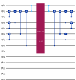
(b) FBS gate.

Figure 7: Left-hand side: logarithmic depth gate computing the parity of the qubits between qubit $0$ and qubit $8$. This parity is stored in qubit $1$. Right-hand side: FBS gate between qubit $0$ and qubit $8$.

The pyramid and parallel architectures are suited for loading dense vectors since they do not adapt to the sparsity structure of $x$. In Section 5.1.1, we propose another architecture called sparse Clifford loaders in order to load vectors such as columns of an edge-vertex incidence matrix of a graph. In that case, the pyramidion of the loader is chosen according to the sparsity pattern of $\mathsf{x}$. The sparse loader of $\mathsf{x}$ requires $\mathrm{nnz}(\mathsf{x})$ two-qubit gates and has $\mathcal{O}(n)$ depth.

5.1.1 Sparse architecture

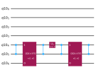
(a) Sparse Clifford loader.

(b) $\mathsf{x}=B_{:4}$

(c) Barbell graph.

Figure 8: Loading the column of the edge-vertex incidence matrix $B$ (barbell graph) corresponding to vertex $4$ with a sparse Clifford architecture made of one FBS gate. In this case, the pyramidion is $\ell_{\triangle}=5$, i.e., edge $(\varrho,4)$.

To construct sparse versions of Clifford loaders, we adapt the strategy of [27]. Namely, Givens rotations are used to zero out – one-by-one – all the non-vanishing entries of the starting vector until this vector has a unique non-vanishing entry.

Index $1\leq\ell_{\triangle}\leq n$ and numerical precision $\mathtt{tol}>0$.

Initialize $\mathsf{x}^{\prime}=\mathsf{x}$ and $\mathcal{U}=\mathbb{I}$.

for  $i=n,\dots,1$ do $\sharp$ loop backward from the end of $\mathsf{x}$.

  if $|\mathsf{x}^{\prime}_{i}|\geq\mathtt{tol}$ then

    Find the largest $j$ s.t. $1\leq j\leq i$ and $|\mathsf{x}^{\prime}_{j}|\geq\mathtt{tol}$.

    if $j=i$ then $\sharp$ pyramidion.

    Set $\ell_{\triangle}=i$ and break.

    else$\sharp$ use $j$ as pivot.

    Find $\theta$ and $x_{\star}$ such that $\sharp$ zero out $\mathsf{x}^{\prime}_{i}$ with nearest $\mathsf{x}^{\prime}_{j}\neq 0$.

$$\begin{bmatrix}x_{\star}\\ 0\end{bmatrix}=\begin{bmatrix}\cos\theta&\sin\theta\\ -\sin\theta&\cos\theta\end{bmatrix}\begin{bmatrix}\mathsf{x}^{\prime}_{j}\\ \mathsf{x}^{\prime}_{i}\end{bmatrix}.$$

    Update $\mathsf{x}^{\prime}_{j}\leftarrow x_{\star}$ and $\mathsf{x}^{\prime}_{i}\leftarrow 0$.

    Update $\mathcal{U}\leftarrow\mathcal{U}_{ij}(\theta)\circ\mathcal{U}$ where $\mathcal{U}_{ij}(\theta)$ is given in 50.       

$\mathcal{C}(\mathsf{x})=\mathcal{U}(c_{\ell_{\triangle}}^{*}+c_{\ell_{\triangle}})\mathcal{U}^{*}$.

Algorithm 4 Sparse Clifford loader of $\mathsf{x}\in\mathbb{R}^{n\times 1}$ with $\|\mathsf{x}\|_{2}=1$.

In Algorithm 4, we describe a procedure where we zero out each non-zero entry of the data vector by using the closest non-zero entry as a pivot. We take $\mathtt{tol}=10^{-8}$ as the numeric threshold to distinguish non-zero entries. Note that, in the context of graphs, small circuits built with the sparse architecture contain much fewer gates as it can be seen from the example of Figure 13 (bottom). This sparse architecture contains $12$ $\mathtt{XX+YY}$ gates and $8$ controlled-$\sigma_{z}$ gates, whereas the parallel architecture contains $20$ $\mathtt{XX+YY}$ gates, $24$ controlled-$\sigma_{z}$ gates and $16$ controlled-$\sigma_{x}$ gates.

5.2 Simulation results

We consider two graphs: a complete graph and a barbell graph, for which the acceptance probability of our algorithm is discussed, respectively, in Example 4.8 and Example 4.9. This determinantal measure over edges is a specific case of the DPP with skewsymmetric $L$-matrix of Theorem 4.1. For these simulations, we sample dimer-rooted forests with and without the amplification circuit described in Section 3.

(a) Complete graph with $\varrho=3$.

(b) Barbell graph with $\varrho=3$.

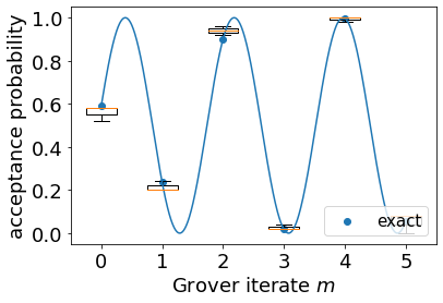
(c) Acceptance vs $m$ (complete graph).

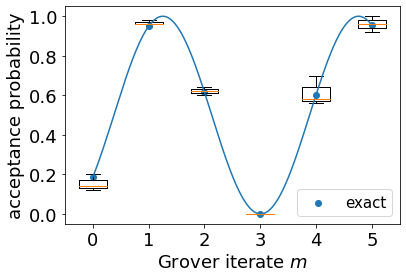
(d) Acceptance vs $m$ (barbell graph).

Figure 9: Effect of amplification on the acceptance probability in Algorithm 2 for sampling determinantal dimer-rooted forests in a complete graph (left-hand side) and a barbell graph (right-hand side). The blue dots denote the exact value of the amplified probability. The boxes are obtained by simulation of a logarithmic Clifford loader. For each $0\leq m\leq 5$, the acceptance frequency is estimated over $50$ independent DPP samples, and error bars are obtained by repeating this estimation $3$ times. The orange curve is the extrapolation of the $\sin^{2}(x)$ function of Remark 3.1.

Although Algorithm 2 determines the number of Grover steps $m$, for an illustrative purpose, we also consider the acceptance probability 28 as a function of $m$. In Figure 9(c) and Figure 9(d), the periodic effect of amplitude amplification 27 – of the form of a $sin^{2}(x)$ function – is made manifest: for the complete graph where the initial acceptance probability is already large, and for boosting the acceptance probability in the case of the barbell graph. As a matter of fact, one Grover iteration ($m=1$) is sufficient to amplify substancially the acceptance probability in the case of the barbell graph (Figure 9(d)) whereas the same number of iterations reduces this probability in the case of the complete graph (Figure 9(c), in which case Algorithm 2 simply chooses $m=0$). Adding several Grover iterations yields to an oscillatory behaviour where amplification as well as reduction can occur.

\begin{overpic}[width=433.62pt,scale={0.055}]{fig/complete_hist_1.png} \put(67.0,14.0){\footnotesize spanning trees} \put(54.0,12.0){\line(1,0){43.0}} \end{overpic}

Figure 10: Simulated subset frequencies (orange) with a parallel Clifford loader vs exact subset probabilities (blue) in the case of the complete graph of $4$ nodes depicted in Figure 9(a). Subset frequencies are estimated over $1000$ independent DPP samples. At the right of the histogram, we observe the equal probability mass given to the spanning trees of the complete graph which are subsets of $3$ edges in this case.

Also, we directly report an estimate of the probability of any subset of edges. Edges are enumerated as follows. An orientation is fixed by writing an edge as $(i,j)$ with $i<j$, and all the edges are then ordered lexicographically; for example, in Figure 9(a), $(0,1)$ is edge $\mathtt{(0,)}$, next $(0,2)$ is edge $\mathtt{(1,)}$, etc. Figure 10 and Figure 11 provide histograms comparing empirical and exact subset probabilities. These plots illustrate the fact that the determinantal measure only gives mass to dimer-rooted forests of odd cardinal since these two graphs have an even number of nodes; see Definition 4.6.

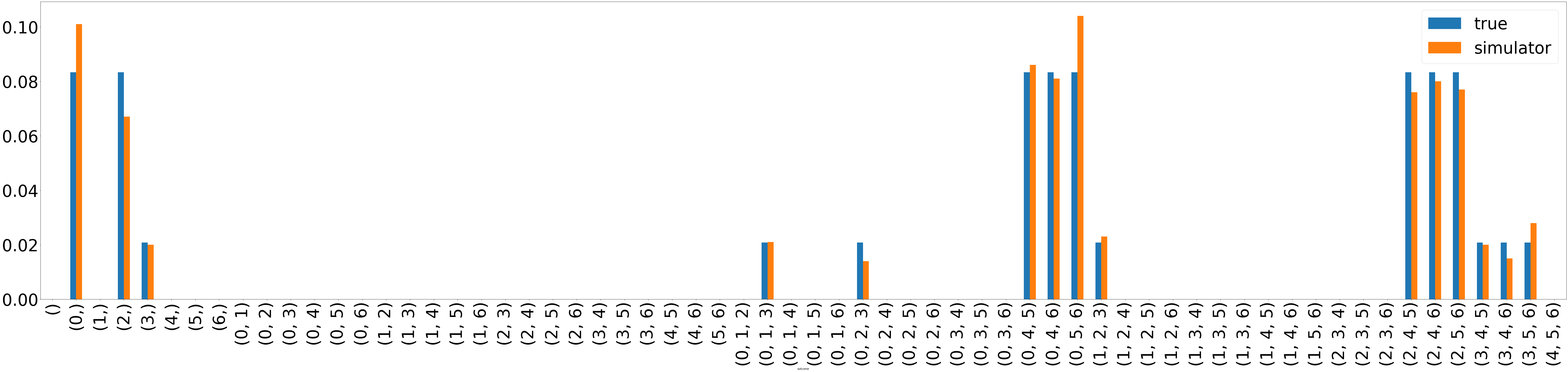
\begin{overpic}[width=433.62pt,scale={0.055}]{fig/barbell_hist_2.png} \put(67.0,15.0){\footnotesize spanning trees} \put(65.0,14.0){\line(1,0){18.0}} \par\end{overpic}

Figure 11: Simulated subset frequencies (orange) with the parallel Clifford loader vs exact subset probabilities (blue) in the case of the barbell graph of $6$ nodes given in Figure 9(b). Subset frequencies are estimated over $1000$ independent DPP samples. At the right of the second row, we observe the equal probability mass given to the spanning trees which are subsets of $5$ edges in this case.

Remark 5.2 (Example of dimer-rooted forests with zero probability).

By inspecting for instance Figure 11, we observe that the edge denoted by $\mathtt{(1,)}$ on the $x$-axis – that is the single edge corresponding to the node pair $(0,2)$ in Figure 9(b) – has zero probability to be sampled. Nonetheless, the single edge $(0,2)$ is a dimer-rooted forest with root $\varrho=3$. This lack of symmetry is a consequence of the orientation induced by the node ordering as we now explain. Indeed, as mentioned in the proof of Theorem 4.7, $C=\mathrm{skew}(L_{\widehat{\varrho}\widehat{\varrho}})$ can be interpreted as a skewsymmetric adjacency matrix. Thus, for all edge $(i,j)$ with $i<j$, we have $C_{ij}=1$ and therefore the edge is oriented from $i$ to $j$, as illustrated in Figure 12(a). Now, by using Theorem 4.7, the probability that $(0,2)$ is sampled equals

$$\det\hbox{}\vbox{\kern 0.86108pt\hbox{$\kern 0.0pt\kern 2.5pt\kern-5.0pt\left[\kern 0.0pt\kern-2.5pt\kern-5.0pt\vbox{\kern-0.86108pt\vbox{\vbox{ \halign{\kern\arraycolsep\hfil\@arstrut$\kbcolstyle#$\hfil\kern\arraycolsep& \kern\arraycolsep\hfil$\@kbrowstyle#$\ifkbalignright\relax\else\hfil\fi\kern\arraycolsep&& \kern\arraycolsep\hfil$\@kbrowstyle#$\ifkbalignright\relax\else\hfil\fi\kern\arraycolsep\cr 5.0pt\hfil\@arstrut$\scriptstyle$\hfil\kern 5.0pt&5.0pt\hfil$\scriptstyle(0,2)$\hfil\kern 5.0pt&5.0pt\hfil$\scriptstyle 0$\hfil\kern 5.0pt&5.0pt\hfil$\scriptstyle 1$\hfil\kern 5.0pt&5.0pt\hfil$\scriptstyle 2\\(0,2)$\hfil\kern 5.0pt&5.0pt\hfil$\scriptstyle 0$\hfil\kern 5.0pt&5.0pt\hfil$\scriptstyle 1$\hfil\kern 5.0pt&5.0pt\hfil$\scriptstyle 0$\hfil\kern 5.0pt&5.0pt\hfil$\scriptstyle-1\\0$\hfil\kern 5.0pt&5.0pt\hfil$\scriptstyle-1$\hfil\kern 5.0pt&5.0pt\hfil$\scriptstyle 0$\hfil\kern 5.0pt&5.0pt\hfil$\scriptstyle 1$\hfil\kern 5.0pt&5.0pt\hfil$\scriptstyle 1\\1$\hfil\kern 5.0pt&5.0pt\hfil$\scriptstyle 0$\hfil\kern 5.0pt&5.0pt\hfil$\scriptstyle-1$\hfil\kern 5.0pt&5.0pt\hfil$\scriptstyle 0$\hfil\kern 5.0pt&5.0pt\hfil$\scriptstyle 1\\2$\hfil\kern 5.0pt&5.0pt\hfil$\scriptstyle 1$\hfil\kern 5.0pt&5.0pt\hfil$\scriptstyle-1$\hfil\kern 5.0pt&5.0pt\hfil$\scriptstyle-1$\hfil\kern 5.0pt&5.0pt\hfil$\scriptstyle 0$\hfil\kern 5.0pt\crcr}}}}\right]$}}=0.$$

Considering the augmented graph of Figure 12(b), the above determinant vanishes since the row of node $(0,2)$ is collinear with the row of node $1$.

(a) $\mathrm{skew}(L_{\widehat{\varrho}\widehat{\varrho}})$.

(b) $\left(\begin{smallmatrix}0&B_{\mathtt{C}\widehat{\varrho}}\\ -(B_{\mathtt{C}\widehat{\varrho}})^{\top}&\mathrm{skew}(L_{\widehat{\varrho}\widehat{\varrho}})\end{smallmatrix}\right)$ with $\mathtt{C}=\{(0,2)\}$.

Figure 12: Oriented graphs associated with two skewsymmetric adjacency matrices obtained in the case of the barbell graph of Figure 9(b); see Remark 5.2.

5.3 Results on Quantum Computing Units

To illustrate the effect of noise, we execute the experiment of Figure 11 (still without amplification) on one of the freely available Quantum Computing Units (QPUs) of IBM Quantum Plateform with $127$ qubits, namely $\mathtt{ibm\_sherbrooke}$, by using this time a sparse Clifford loader.

Concerning the timing, $8192$ samples were obtained in about $4s$ excluding transpilation time, according to IBM Quantum Plateform dashboard. The frequencies of sampled subsets are displayed in Figure 13. In the first two rows of Figure 13, the subsets with large probabilities are indeed sampled although other subsets with vanishing probability also appear due to the presence of noise. Note that we used the highest possible level of optimization of the transpiler, namely $\mathtt{optimization\_level}=3$, in order to reduce the errors as much as possible. The results without optimization ($\mathtt{optimization\_level}=0$) are more noisy as it can be seen in Figure 14.

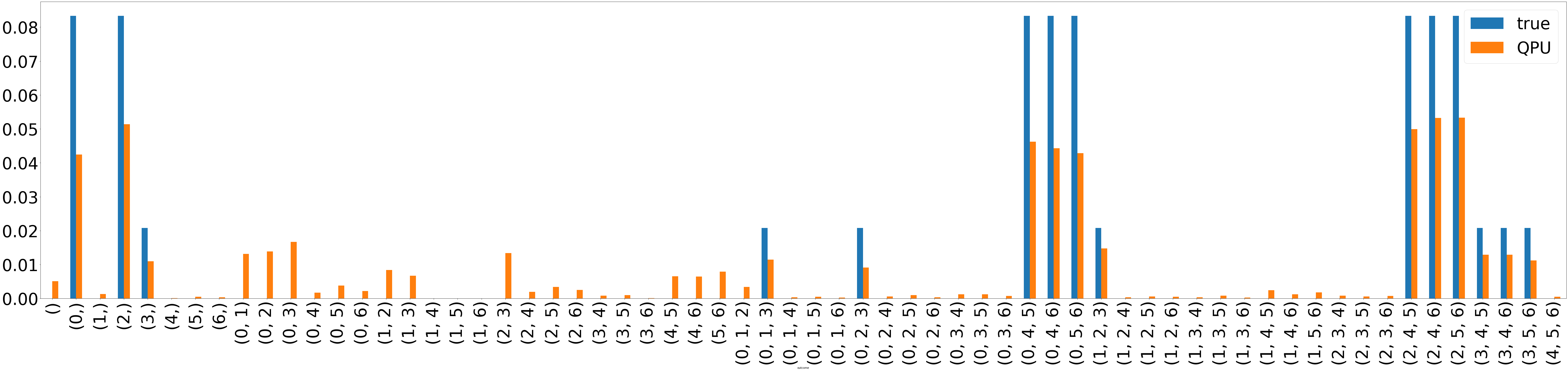
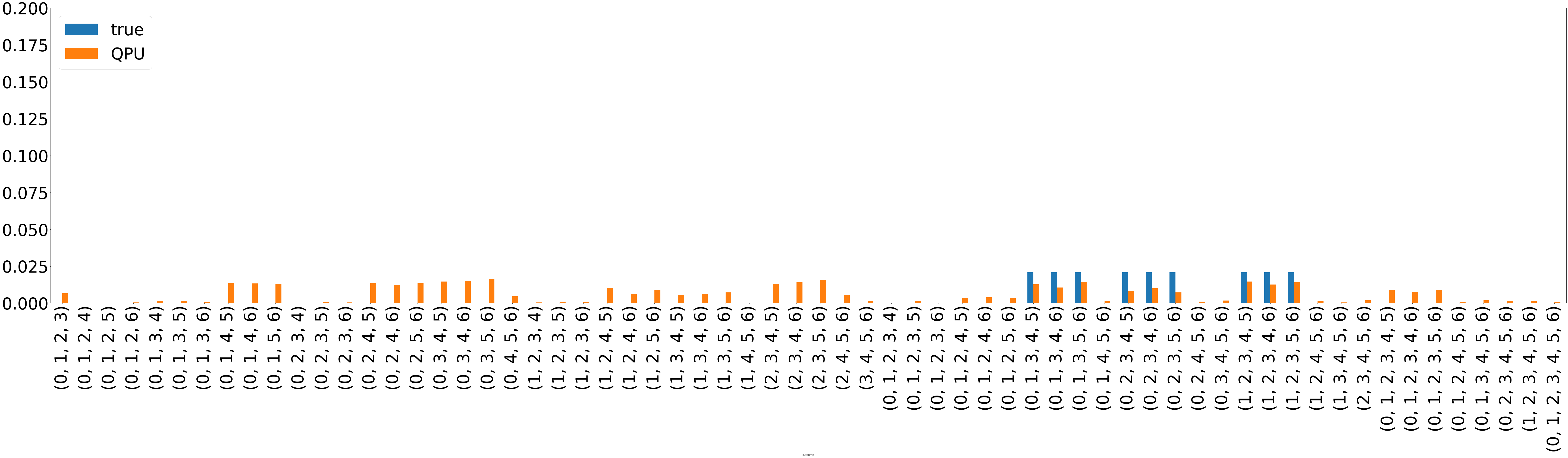
Figure 13: Row $1$ and Row $2$: observed subset frequencies on $\mathtt{ibm\_sherbrooke}$ (orange) with the sparse Clifford loader vs exact subset probabilities (blue) in the case of the barbell graph of Figure 9(b). Row 3: the corresponding sparse Clifford loader with FBS gates. Subset frequencies are estimated over $8192$ independent DPP samples. Qiskit transpiler is used with the option $\mathtt{optimization\_level}=3$.

In general, we found that the parallel and sparse architectures – which use FBS gates – are more error prone than the pyramid architecture. The reason might be that the latter only use RBS gates on neighbouring qubits, while the former use additional controlled-$\sigma_{z}$ and controlled-$\sigma_{x}$ gates; see Figure 7 for an example.

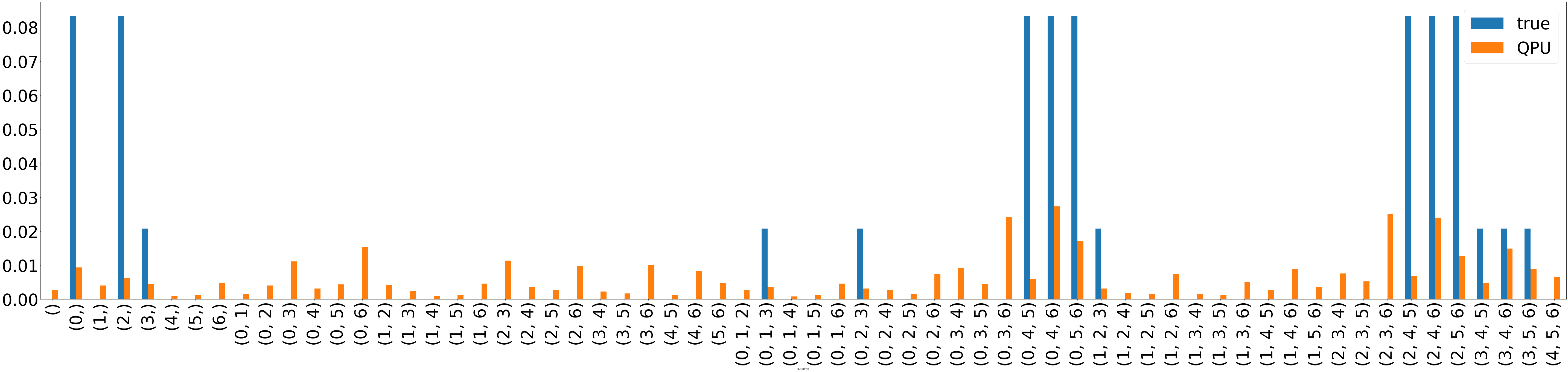
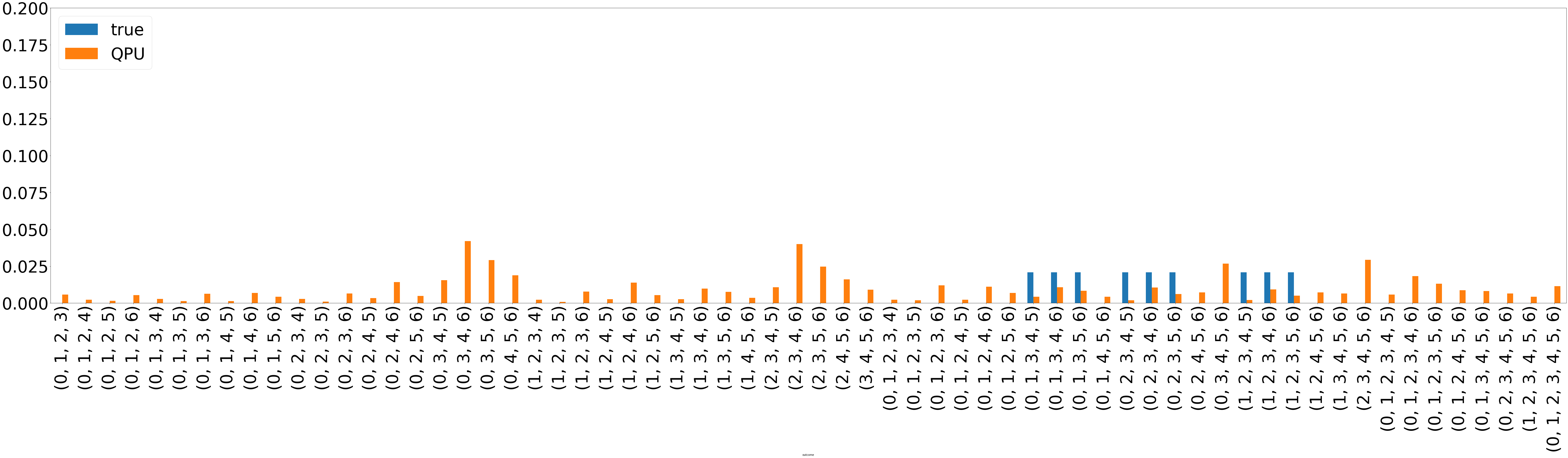
Figure 14: Row $1$ and Row $2$: observed subset frequencies on $\mathtt{ibm\_sherbrooke}$ (orange) with the sparse Clifford loader vs exact subset probabilities (blue) in the case of the barbell graph of Figure 9(b). In contrast with Figure 13, the Qiskit transpiler uses the lowest optimization level, i.e., $\mathtt{optimization\_level}=0$.

6 Conclusion

We have presented an algorithm that samples a DPP when the kernel is a projection onto a space given by a non-orthonormal spanning set of vectors, namely the columns of the $n\times r$ matrix $X$. The computational bottleneck of our algorithm is a classical preprocessing step that approximates $\det\mathsf{X}^{\top}\mathsf{X}$. Whenever this step is $o(nr^{2})$, we have a faster DPP sampling algorithm than classical counterparts.

Our algorithm takes the form of a classical preprocessing through a normalization step and an estimation of the necessary number of Grover steps, followed by a bounded number of repeated runs of a quantum circuit until an easily-checked cardinality constraint is met. In passing, we have characterized the distribution of the output of our algorithm when only one run of the circuit is performed, without checking the cardinality constraint. This side contribution sheds light on the robustness of a previous algorithm by [31] and brings a new DPP forward, by identifying a DPP kernel of a type unknown in previous applications of DPPs, yet that is natural in the quantum formalization of DPPs. We have illustrated our algorithm on small-scale graph examples, which also shows the potential of our algorithm is numerical applications of uniform spanning trees and related distributions. This connects our approach to recent work by [2], who propose a quantum algorithm for graph sparsification that assumes a QRAM memory and does not explicitly sample uniform spanning trees.

There are many potential extensions of our algorithm. For instance, one could design DPP-specific error-correcting codes, using known statistical properties of DPPs to detect e.g. readout errors. We could also adapt our circuit to the particular machine on which it is run, by taking into account the estimated accuracies of one- and two-qubit gates provided by the constructor. This is partially done automatically when running circuits e.g. on IBM machines, a step known as transpilation, but the procedure could be taylored to our particular task. More formally, it would also be interesting to define Clifford loaders in order to sample quaternionic DPPs [29] or the recently introduced multideterminantal DPPs [30].

Other interesting avenues for future work are the completion of our quantum circuit to treat a downstream task such as linear regression with column subset selection directly on the quantum computer, instead of outputting a DPP sample. Moreover, it would be interesting to see if other QR-related numerical algebraic tasks than DPP sampling can benefit from the combination of Clifford loaders and amplitude rejection.

Appendix A Clifford loaders

We revisit here the construction of Clifford loaders by [28] and [31] with the operator algebra approach of [4]; see Section A.1.

A.1 Parallel and pyramid architectures

In the next subsection, we highlight a connection – which is implicit in [31] – between the Clifford loaders and spherical coordinate systems.

A.1.1 Spherical coordinate systems

The basic idea to construct $\mathcal{U}(\mathsf{x})$ in 46 is to use spherical coordinates of $\mathsf{x}$. We can consider the case where $n$ is a power of $2$ since any vector can be increased in length by adding zeros so that its length is $2^{k}$ for some $k$. Hyperspherical coordinate systems of $\mathsf{x}$ are associated with binary trees, as it is explained in [37, Chapter 6]. Following [28], we are interested in circuits with short depth which are associated with binary trees of short depth where parallel operations are executed. We give an example of this parallelism for $n=4$ in Figure 15, so that the generalization to higher $n$ becomes intuitive.

Figure 15: Hyperspherical coordinates of a unit norm $\mathsf{x}\in\mathbb{R}^{4}$ (parallel shape). For simplicity, we assume that none of the components of $\mathsf{x}$ vanish. The parameters $r_{3},r_{2},r_{1}$ are obtained by going along the tree from the leafs to the root. The angles $\theta_{1},\theta_{2},\theta_{3}$ are computed by going from the root to the leafs and using $r_{1},r_{2},r_{3}$.

To compute the spherical coordinates of $\mathsf{x}$, we go in the tree from the leafs to the roots to evaluate the $r_{i}$s. Next, the angles $\theta_{i}$s are obtained by visiting the nodes from the root to the leaves. We see that the computation of all the coordinates of $\mathsf{x}$ requires $\mathcal{O}(n)$ operations. Note that different binary trees correspond to different spherical coordinate systems. For example, for $\mathsf{x}\in\mathbb{R}^{8}$, the tree of largest depth (i.e., least parallel) is given in Figure 16.

Figure 16: Hyperspherical coordinates of a unit vector $\mathsf{x}\in\mathbb{R}^{8}$ with pyramid shape. Again, we assume that none of the components of $\mathsf{x}$ vanish.

A.1.2 RBS gates

We now give the intuition behind the use of the Givens operator to load a unit vector in $\mathbb{R}^{4}$ with parallel rotations as in the case of the tree of Figure 15. Consider the vector $\mathsf{y}=[\cos\theta,\sin\theta,0,0]^{\top}.$ Actually, there exists a unitary operator $\mathcal{U}(\mathsf{y})$ – called here Givens operator – such that $\mathcal{U}\ket{\emptyset}=\ket{\emptyset}$ and

$$\begin{bmatrix}\mathcal{U}\ c_{1}^{*}\ \mathcal{U}^{*}\\ \mathcal{U}\ c_{2}^{*}\ \mathcal{U}^{*}\end{bmatrix}=\begin{bmatrix}\cos\theta&\sin\theta\\ -\sin\theta&\cos\theta\end{bmatrix}\begin{bmatrix}c_{1}^{*}\\ c_{2}^{*}\end{bmatrix}\text{ and }\mathcal{U}c_{i}^{*}\mathcal{U}^{*}=c_{i}^{*},\quad\forall i\notin\{1,2\};$$ (48)

as defined e.g. in [4, Section 5.2.1]. We can load $\mathsf{y}$ by acting on the Fock vacuum as follows:

$$\mathcal{C}(\mathsf{y})\ket{\emptyset}=\cos\theta\ c_{1}^{*}\ket{\emptyset}+\sin\theta\ c_{2}^{*}\ket{\emptyset}.$$

In the computational basis, this reads $\mathcal{C}(\mathsf{y})\ket{0000}=\cos\theta\ket{1000}+\sin\theta\ket{0100}.$ The following result – whose proof is elementary – is used in order to implement Clifford loaders whenever qubits are consecutive.

Lemma A.1 (RBS Gate).

Let $\mathcal{U}$ be the operator defined in 48. Consider the vector space generated by the following orthonormal basis:

$$\left(\ket{\emptyset}=\ket{0000},c_{1}^{*}\ket{\emptyset}=\ket{1000},c_{2}^{*}\ket{\emptyset}=\ket{0100},c_{2}^{*}c_{1}^{*}\ket{\emptyset}=\ket{1100}\right).$$

Denote this basis by $\mathcal{B}$. The representation of $\mathcal{U}$ restricted to this subspace is

$$\rho(\mathcal{U})_{\mathcal{B}\mathcal{B}}=\hbox{}\vbox{\kern 0.86108pt\hbox{$\kern 0.0pt\kern 2.5pt\kern-5.0pt\left[\kern 0.0pt\kern-2.5pt\kern-5.0pt\vbox{\kern-0.86108pt\vbox{\vbox{ \halign{\kern\arraycolsep\hfil\@arstrut$\kbcolstyle#$\hfil\kern\arraycolsep& \kern\arraycolsep\hfil$\@kbrowstyle#$\ifkbalignright\relax\else\hfil\fi\kern\arraycolsep&& \kern\arraycolsep\hfil$\@kbrowstyle#$\ifkbalignright\relax\else\hfil\fi\kern\arraycolsep\cr 5.0pt\hfil\@arstrut$\scriptstyle$\hfil\kern 5.0pt&5.0pt\hfil$\scriptstyle\ket{0000}$\hfil\kern 5.0pt&5.0pt\hfil$\scriptstyle\ket{1000}$\hfil\kern 5.0pt&5.0pt\hfil$\scriptstyle\ket{0100}$\hfil\kern 5.0pt&5.0pt\hfil$\scriptstyle\ket{1100}\\\ket{0000}$\hfil\kern 5.0pt&5.0pt\hfil$\scriptstyle 1$\hfil\kern 5.0pt&5.0pt\hfil$\scriptstyle 0$\hfil\kern 5.0pt&5.0pt\hfil$\scriptstyle 0$\hfil\kern 5.0pt&5.0pt\hfil$\scriptstyle 0\\\ket{1000}$\hfil\kern 5.0pt&5.0pt\hfil$\scriptstyle 0$\hfil\kern 5.0pt&5.0pt\hfil$\scriptstyle\cos\theta$\hfil\kern 5.0pt&5.0pt\hfil$\scriptstyle\sin\theta$\hfil\kern 5.0pt&5.0pt\hfil$\scriptstyle 0\\\ket{0100}$\hfil\kern 5.0pt&5.0pt\hfil$\scriptstyle 0$\hfil\kern 5.0pt&5.0pt\hfil$\scriptstyle-\sin\theta$\hfil\kern 5.0pt&5.0pt\hfil$\scriptstyle\cos\theta$\hfil\kern 5.0pt&5.0pt\hfil$\scriptstyle 0\\\ket{1100}$\hfil\kern 5.0pt&5.0pt\hfil$\scriptstyle 0$\hfil\kern 5.0pt&5.0pt\hfil$\scriptstyle 0$\hfil\kern 5.0pt&5.0pt\hfil$\scriptstyle 0$\hfil\kern 5.0pt&5.0pt\hfil$\scriptstyle 1$\hfil\kern 5.0pt\crcr}}}}\right]$}},$$ (49)

whereas $\rho(\mathcal{U})$ is the identity in the subspace generated by $\ket{0010}$ and $\ket{0001}$. The matrix 49 is called in [31] a Reconfigurable Beam Splitter (RBS) gate.

Roughly speaking, a RBS represents a Givens operator in the one-particle subspace. Considering now a space of $n$ qubits, we denote the operator acting in the subspace of the $i$th and $j$th qubits as 49 by $\mathrm{RBS}_{ij}(\theta)$ with $1\leq i<j\leq n$. This gate can be realized in Qiskit by a $\mathtt{XX+YY}$ gate.

A.1.3 FBS gates

In Lemma A.2 below, we formalize a result by [31] which describes the Givens operator in a subspace with more than one particle.

Lemma A.2 (FBS Gate).

Consider the setting of Lemma A.1. Let $1\leq i<j\leq n$ and denote by $\mathcal{U}_{ij}(\theta)$ the operator defined by $\mathcal{U}_{ij}(\theta)\ket{\emptyset}=\ket{\emptyset}$,

$$\begin{bmatrix}\mathcal{U}_{ij}(\theta)\ c_{i}^{*}\ \mathcal{U}_{ij}(\theta)^{*}\\ \mathcal{U}_{ij}(\theta)\ c_{j}^{*}\ \mathcal{U}_{ij}(\theta)^{*}\end{bmatrix}=\begin{bmatrix}\cos\theta&\sin\theta\\ -\sin\theta&\cos\theta\end{bmatrix}\begin{bmatrix}c_{i}^{*}\\ c_{j}^{*}\end{bmatrix}\text{ and }\mathcal{U}_{ij}(\theta)c_{k}^{*}\mathcal{U}_{ij}(\theta)^{*}=c_{k}^{*},\ \forall k\notin\{i,j\}.$$ (50)

For any ordered subset $\mathtt{C}$, we denote by $\ket{\mathtt{C}}$ the state of the computational basis representing $\prod_{k\in\mathtt{C}}c_{k}^{*}\ket{\emptyset}$ in the Jordan-Wigner representation. Let $\mathtt{S}$ be an ordered subset of $\{1,\dots,n\}$ such that $i,j\in\mathtt{S}$. Denote by $\mathcal{B}$ the orthonormal basis

$$\left(\ket{\mathtt{S}},\ket{\mathtt{S}\setminus i},\ket{\mathtt{S}\setminus j},\ket{\mathtt{S}\setminus\{i,j\}}\right).$$

The representation of $\mathcal{U}$ restricted to this subspace is

$$\rho(\mathcal{U})_{\mathcal{B}\mathcal{B}}=\hbox{}\vbox{\kern 0.86108pt\hbox{$\kern 0.0pt\kern 2.5pt\kern-5.0pt\left[\kern 0.0pt\kern-2.5pt\kern-5.0pt\vbox{\kern-0.86108pt\vbox{\vbox{ \halign{\kern\arraycolsep\hfil\@arstrut$\kbcolstyle#$\hfil\kern\arraycolsep& \kern\arraycolsep\hfil$\@kbrowstyle#$\ifkbalignright\relax\else\hfil\fi\kern\arraycolsep&& \kern\arraycolsep\hfil$\@kbrowstyle#$\ifkbalignright\relax\else\hfil\fi\kern\arraycolsep\cr 5.0pt\hfil\@arstrut$\scriptstyle$\hfil\kern 5.0pt&5.0pt\hfil$\scriptstyle\ket{\mathtt{S}}$\hfil\kern 5.0pt&5.0pt\hfil$\scriptstyle\ket{\mathtt{S}\setminus i}$\hfil\kern 5.0pt&5.0pt\hfil$\scriptstyle\ket{\mathtt{S}\setminus j}$\hfil\kern 5.0pt&5.0pt\hfil$\scriptstyle\ket{\mathtt{S}\setminus\{i,j\}}\\\ket{\mathtt{S}}$\hfil\kern 5.0pt&5.0pt\hfil$\scriptstyle 1$\hfil\kern 5.0pt&5.0pt\hfil$\scriptstyle 0$\hfil\kern 5.0pt&5.0pt\hfil$\scriptstyle 0$\hfil\kern 5.0pt&5.0pt\hfil$\scriptstyle 0\\\ket{\mathtt{S}\setminus i}$\hfil\kern 5.0pt&5.0pt\hfil$\scriptstyle 0$\hfil\kern 5.0pt&5.0pt\hfil$\scriptstyle\cos\theta$\hfil\kern 5.0pt&5.0pt\hfil$\scriptstyle(-1)^{f(i,j,\mathtt{S})}\sin\theta$\hfil\kern 5.0pt&5.0pt\hfil$\scriptstyle 0\\\ket{\mathtt{S}\setminus j}$\hfil\kern 5.0pt&5.0pt\hfil$\scriptstyle 0$\hfil\kern 5.0pt&5.0pt\hfil$\scriptstyle(-1)^{1+f(i,j,\mathtt{S})}\sin\theta$\hfil\kern 5.0pt&5.0pt\hfil$\scriptstyle\cos\theta$\hfil\kern 5.0pt&5.0pt\hfil$\scriptstyle 0\\\ket{\mathtt{S}\setminus\{i,j\}}$\hfil\kern 5.0pt&5.0pt\hfil$\scriptstyle 0$\hfil\kern 5.0pt&5.0pt\hfil$\scriptstyle 0$\hfil\kern 5.0pt&5.0pt\hfil$\scriptstyle 0$\hfil\kern 5.0pt&5.0pt\hfil$\scriptstyle 1$\hfil\kern 5.0pt\crcr}}}}\right]$}},$$ (51)

where $f(i,j,\mathtt{S})=\sum_{i<k<j:k\in\mathtt{S}}1$. Furthermore, $\rho(\mathcal{U}_{ij}(\theta))\ket{\mathtt{S}^{\prime}}=\ket{\mathtt{S}^{\prime}}$ for all $\mathtt{S}^{\prime}$ such that $i,j\notin\mathtt{S}^{\prime}$. We denote the operator acting in the subspace of the $i$th and $j$th qubits as 51 by $\mathrm{FBS}_{ij}(\theta)$ with $1\leq i<j\leq n$.

The above matrix is called in [31] a Fermionic Beam Splitter (FBS) gate. The only difference with Lemma A.1 is the possible presence of an extra minus sign which is due to the (fermionic) anticommutation relations and counts the parity of the number of particles between $i$ and $j$. In our understanding, this is why this gate is called fermionic.

For completeness, we give a sketch of proof of Lemma A.2.

Sketch of proof of Lemma A.2.

We compute $\mathcal{U}\ket{\mathtt{S}\setminus i}$. To begin, we observe that

$$\ket{\mathtt{S}\setminus i}=\left(\prod_{k\in\mathtt{S}:k<i}c^{*}_{k}\right)\left(\prod_{k\in\mathtt{S}:i<k<j}c^{*}_{k}\right)c_{j}^{*}\left(\prod_{k\in\mathtt{S}:k>j}c_{k}^{*}\right)\ket{\emptyset}.$$

Now, by applying $\mathcal{U}$, we find

$$\mathcal{U}\ket{\mathtt{S}\setminus i} =\left(\prod_{k\in\mathtt{S}:k<i}c^{*}_{k}\right)\left(\prod_{k\in\mathtt{S}:i<k<j}c^{*}_{k}\right)\mathcal{U}c_{j}^{*}\mathcal{U}^{*}\mathcal{U}\left(\prod_{k\in\mathtt{S}:k>j}c_{k}^{*}\right)\ket{\emptyset}$$

$$=\left(\prod_{k\in\mathtt{S}:k<i}c^{*}_{k}\right)\left(\prod_{k\in\mathtt{S}:i<k<j}c^{*}_{k}\right)\left(-\sin\theta c_{i}^{*}+\cos\theta c_{j}^{*}\right)\left(\prod_{k\in\mathtt{S}:k>j}c_{k}^{*}\right)\ket{\emptyset}.$$

Finally, the anticommutation relations on the first term on the right-hand side yields

$$-\sin\theta\left(\prod_{k\in\mathtt{S}:k<i}c^{*}_{k}\right)(-1)^{f(i,j,\mathtt{S})}c_{i}^{*}\left(\prod_{k\in\mathtt{S}:i<k<j}c^{*}_{k}\right)\left(\prod_{k\in\mathtt{S}:k>j}c_{k}^{*}\right)\ket{\emptyset}.$$

Thus, the desired result is

$$\mathcal{U}\ket{\mathtt{S}\setminus i}=-(-1)^{f(i,j,\mathtt{S})}\sin\theta\ket{\mathtt{S}\setminus j}+\cos\theta\ket{\mathtt{S}\setminus i},$$

where $f(i,j,\mathtt{S})$ is the cardinal of $\{k\in\mathtt{S}:i<k<j\}$. ∎

Next, in order to make this paper more self-contained, we slightly rephrase [31, Proposition 2.6] which gives a decomposition of FBS gates.

An FBS gate between qubits $i$ and $j$ can be realized by combining RBS gates with gates computing the parity of the intermediate qubits. Let $j>i+1$ to avoid trivial cases. Denote by $\mathrm{CZ}_{i,j}$ the controlled-$\sigma_{z}$ gate between $i$ and $j$. Let $P_{i+1,j}$ be the parity gate computing the parity of the qubits between $i$ and $j$ and storing it in qubit $i+1$; see Figure 7(a) for an illustration. This gate is constructed with controlled-$\sigma_{x}$ gates and has log-depth. For all $1\leq i<j\leq n$, we have

$$\mathrm{FBS}_{ij}(\theta)=P_{i+1,j}\mathrm{CZ}_{i,i+1}\mathrm{RBS}_{ij}(\theta)\mathrm{CZ}_{i,i+1}P_{i+1,j}^{*}.$$

Appendix B Useful technical results

The following proposition is a consequence of Wick’s theorem.

Proposition B.1.

Let $k$ be an even integer and let $\mathsf{X}\in\mathbb{R}^{n\times k}$ have linearly independent columns of unit $2$-norm. If $k$ is even, we have

$$\innerproduct{0}{\mathrm{columns}(\mathsf{X})}=\mathrm{pf}\left(\mathrm{skew}(\mathsf{X}^{\top}\mathsf{X})\right).$$

In particular, if $\mathsf{X}\in\mathbb{R}^{n\times r}$ and $\mathsf{X}^{\prime}\in\mathbb{R}^{n\times r^{\prime}}$ have linearly independent columns of unit $2$-norm and are such that $\text{parity}(r)=\text{parity}(r^{\prime})$, we have

$$\innerproduct{\mathrm{columns}(\mathsf{X}^{\prime})}{\mathrm{columns}(\mathsf{X})}=\mathrm{pf}\begin{bmatrix}\mathrm{skew}(\mathsf{X}^{\top}\mathsf{X})&\mathsf{X}^{\top}\mathsf{X}^{\prime}\\ -\mathsf{X}^{\prime\top}\mathsf{X}&\mathrm{skew}(\mathsf{X}^{\prime\top}\mathsf{X}^{\prime}).\end{bmatrix}$$

Otherwise, if $\text{parity}(r)\neq\text{parity}(r^{\prime})$, it holds that $\innerproduct{\mathrm{columns}(\mathsf{X}^{\prime})}{\mathrm{columns}(\mathsf{X})}=0$.

Proof.

We use Wick’s theorem – see e.g. Theorem 3 in [6] and references therein – and the contraction $\bra{\emptyset}\mathcal{C}(\mathsf{x})\mathcal{C}(\mathsf{x}^{\prime})\ket{\emptyset}=\mathsf{x}^{\top}\mathsf{x}^{\prime}$ as a consequence of 5. ∎

As a consequence of Proposition B.1, if the columns of $\mathsf{X}$ are also orthogonal and $r^{\prime}=r$, we recover that $\innerproduct{\mathrm{columns}(\mathsf{X}^{\prime})}{\mathrm{columns}(\mathsf{X})}\propto\det(\mathsf{X}^{\top}\mathsf{X}^{\prime})$ by using e.g. Lemma B.2. The latter determinant can be expressed in terms of the product of cosines of principal angles between the vector spaces $\text{col}(\mathsf{X})$ and $\text{col}(\mathsf{X}^{\prime})$; see [31, page 10].

B.1 Expression of $\ket{\mathrm{columns}(\mathsf{X})}$

To determine the expression of the coefficient in front of the basis vector $c_{s_{\ell}}^{*}\dots c_{s_{1}}^{*}\ket{\emptyset}$ in the decomposition 35 of $\ket{\mathrm{columns}(\mathsf{X})}$, we use the version of Wick’s Theorem in [6, Section 3.5] with respect to the Fock vacuum $\ket{\emptyset}$. A particular case is the following: consider linear combinations of the $c_{i}$’s and $c_{i}^{*}$’s (defined in CAR) that we denote $\beta_{1},\dots,\beta_{m}$ where $m$ is even. Then, we have

$$\bra{\emptyset}\beta_{1}\dots\beta_{m}\ket{\emptyset}=\sum_{\sigma\text{ contraction}}\mathrm{sgn}(\sigma)\bra{\emptyset}\beta_{\sigma(1)}\beta_{\sigma(2)}\ket{\emptyset}\dots\bra{\emptyset}\beta_{\sigma(m-1)}\beta_{\sigma(m)}\ket{\emptyset}.$$ (52)

We quickly remind the definition of a contraction. For $m$ even, we remind a contraction is a permutation such that $\sigma(1)<\sigma(3)<...<\sigma(m-1)$, and $\sigma(2i-1)<\sigma(2i)$ for $i\leq m/2$. The key point to notice is that the Pfaffian of a skewsymmetric matrix $A\in\mathbb{C}^{2k\times 2k}$ reads

$$\mathrm{pf}(A)=\sum_{\sigma\text{ contraction}}\mathrm{sgn}(\sigma)A_{\sigma(1)\sigma(2)}\dots A_{\sigma(2k-1)\sigma(2k)}.$$ (53)

At this point, we use the following identities:

$$\bra{\emptyset}\mathcal{C}(\mathsf{x})\mathcal{C}(\mathsf{x}^{\prime})\ket{\emptyset}=\mathsf{x}^{\top}\mathsf{x}^{\prime}\text{ and }\bra{\emptyset}\mathcal{C}(\mathsf{x})c_{s}^{*}\ket{\emptyset}=\mathsf{x}_{s}.$$ (54)

Trivially, $\bra{\emptyset}c_{s}c_{s^{\prime}}\ket{\emptyset}=0$. Now, we fix the ordered subset $\mathtt{S}=(s_{1},\dots,s_{\ell})$ and note that $\prod_{i\in\mathrm{rev}(\mathtt{S})}c_{i}^{*}\ket{\emptyset}=c^{*}_{s_{\ell}}\dots c^{*}_{s_{1}}\ket{\emptyset}$. We consider the expression of

$$\bra{\emptyset}c_{s_{1}}\dots c_{s_{\ell}}\mathcal{C}(\mathsf{X}_{:1})\dots\mathcal{C}(\mathsf{X}_{:r})\ket{\emptyset},$$ (55)

in the light of 52.

We define now a skewsymmetric matrix as follows. For $i<j$, we have

$$A_{ij}=\begin{cases}\bra{\emptyset}c_{s_{i}}c_{s_{j}}\ket{\emptyset}&\text{ if }1\leq i<j\leq\ell\\ \bra{\emptyset}c_{s_{i}}\mathcal{C}(\mathsf{X}_{:(j-\ell)})\ket{\emptyset}&\text{ if }1\leq i\leq\ell\text{ and }1\leq j-\ell\leq r\\ \bra{\emptyset}\mathcal{C}(\mathsf{X}_{:(i-\ell)})\mathcal{C}(\mathsf{X}_{:(j-\ell)})\ket{\emptyset}&\text{ if }1\leq i-\ell<j-\ell\leq r\end{cases}.$$

By using 54 and completing the lower triangular part of $A$ to ensure its skewsymmetry, we find

$$A=\begin{bmatrix}0_{\ell}&\mathsf{X}_{\mathtt{S}:}\\ -(\mathsf{X}^{\top})_{:\mathtt{S}}&\mathrm{skew}(\mathsf{X}^{\top}\mathsf{X})\end{bmatrix}.$$

And thus, $\bra{\emptyset}c_{s_{1}}\dots c_{s_{\ell}}\mathcal{C}(\mathsf{X}_{:1})\dots\mathcal{C}(\mathsf{X}_{:r})\ket{\emptyset}=\mathrm{pf}A$. This completes the proof.

B.2 Pfaffian identities

Lemma B.2.

Let $S,X$ be $r\times r$ real matrices with $S^{\top}=-S$. We have

$$\mathrm{pf}\begin{bmatrix}0_{r}&X\\ -X^{\top}&S\end{bmatrix}=(-1)^{r(r-1)/2}\det(X).$$

Proof.

We readily check the identity

$$\begin{bmatrix}0_{r}&X\\ -X^{\top}&S\end{bmatrix}=\begin{bmatrix}0_{r}&-X\\ I_{r}&-S/2\end{bmatrix}\begin{bmatrix}0_{r}&I_{r}\\ -I_{r}&0_{r}\end{bmatrix}\begin{bmatrix}0_{r}&I_{r}\\ -X^{\top}&S/2\end{bmatrix}.$$

Now, we use the well-known formula $\mathrm{pf}(T^{\top}ST)=\det(T)\mathrm{pf}(S)$ where $S$ is skewsymmetric, which gives

$$\mathrm{pf}\begin{bmatrix}0_{r}&X\\ -X^{\top}&S\end{bmatrix}=\det\begin{bmatrix}0_{r}&-X\\ {I_{r}}&-S/2\end{bmatrix}\mathrm{pf}\begin{bmatrix}0_{r}&{I_{r}}\\ -{I_{r}}&0_{r}\end{bmatrix}.$$

Note that, by computing the signature of the appropriate permutation, we have

$$\mathrm{pf}\begin{bmatrix}0_{r}&I_{r}\\ -I_{r}&0_{r}\end{bmatrix}=(-1)^{r(r-1)/2}.$$

The last step is to use

$$\det\begin{bmatrix}A&B\\ C&D\end{bmatrix}=\det(AD-BC)$$

where $A,B,C,D$ has the same size and $C,D$ commute. Since the identity matrix trivially commutes with $-S/2$, we obtain

$$\mathrm{pf}\begin{bmatrix}0_{r}&X\\ -X^{\top}&S\end{bmatrix}=(-1)^{r(r-1)/2}\det\begin{bmatrix}0_{r}&-X\\ I_{r}&-S/2\end{bmatrix}=(-1)^{r(r-1)/2}\det(X).$$

∎

B.3 More about the correlation kernel

Though it is guaranteed by construction, we explicitly prove that the correlation kernel of this DPP has non-negative minors.

Lemma B.3.

Let the assumptions of Theorem 4.2 hold. Let

$$K=X\left(A+X^{\top}X\right)^{-1}X^{\top}.$$

The matrix $K$ is such that $v^{\top}Kv\geq 0$ for all unit norm $v\in\mathbb{R}^{n}$.

Proof.

We actually show that $v^{\top}(K+K^{\top})v\geq 0$. It is sufficient to show that $(A+X^{\top}X)^{-1}$ is positive semi-definite. We rather consider

$$(A+X^{\top}X)^{-1}=(X^{\top}X)^{-1/2}(S+{I_{r}})^{-1}(X^{\top}X)^{-1/2},$$

where $S=(X^{\top}X)^{-1/2}A(X^{\top}X)^{-1/2}$ is skewsymmetric. Now, adding its transpose to $(S+{I_{r}})^{-1}$, we have

$$(S+{I_{r}})^{-1}+(-S+{I_{r}})^{-1} =(-S+{I_{r}}+S+{I_{r}})(S+{I_{r}})^{-1}(-S+{I_{r}})^{-1}$$

$$=2(S+{I_{r}})^{-1}(-S+{I_{r}})^{-1}$$

$$=2(S+{I_{r}})^{-1}(S+{I_{r}})^{\top-1}$$

Hence, by a direct substitution, we find that

$$(K+K^{\top})/2 =X(X^{\top}X)^{-1/2}(S+{I_{r}})^{-1}(S+{I_{r}})^{\top-1}(X^{\top}X)^{-1/2}X^{\top}$$

is manifestly positive semidefinite. ∎

We now explain how Lemma B.3 yields a condition of the principal minors of $K$. Let us use the following lemma.

Lemma B.4 (Lemma 1 in [20]).

Let $A$ be a square real matrix. If $A+A^{\top}$ is positive semidefinite, all principal minors of $A$ are non-negative.

Proof.

This follows from [46, generating method 4.2] which shows that if a real square matrix $A$ is such that $A+A^{\top}$ is strictly positive definite, then all its principal minors are strictly positive. The desired result for the positive semidefinite case follows by using a density argument; see supplementary material of [20] for a complete proof. ∎

References

- [1] N. Anari, Y.P. Liu and T.-D. Vuong “Optimal Sublinear Sampling of Spanning Trees and Determinantal Point Processes via Average-Case Entropic Independence” In SIAM Journal on Computing SIAM, 2024, pp. FOCS22–93 URL: https://doi.org/10.1109/FOCS54457.2022.00019
- [2] S. Apers and R. De Wolf “Quantum Speedup for Graph sparsification, Cut Approximation, and Laplacian Solving” In SIAM Journal on Computing 51.6 SIAM, 2022, pp. 1703–1742 URL: https://doi.org/10.1137/21M1391018
- [3] J. Baez “The Octonions” In Bulletin of the American Mathematical Society 39.2, 2002, pp. 145–205 URL: https://doi.org/10.48550/arXiv.math/0105155
- [4] R. Bardenet, M. Fanuel and A. Feller “On Sampling Determinantal and Pfaffian Point Processes on a Quantum Computer” In Journal of Physics A: Mathematical and Theoretical 57.5 IOP Publishing, 2024, pp. 055202 URL: https://arxiv.org/abs/2305.15851
- [5] R. Bardenet, S. Ghosh and M. Lin “Determinantal Point Processes Based on Orthogonal Polynomials for Sampling Minibatches in SGD” In Advances in Neural Information Processing Systems (NeurIPS), 2021 URL: https://doi.org/10.48550/arXiv.2112.06007
- [6] R. Bardenet et al. “From Point Processes to Quantum Optics and Back” In arXiv:2210.05522, 2022 URL: https://arxiv.org/abs/2210.05522
- [7] S. Barthelmé, N. Tremblay and P.-O. Amblard “A Faster Sampler for Discrete Determinantal Point Processes” In Proceedings of The 26th International Conference on Artificial Intelligence and Statistics 206, Proceedings of Machine Learning Research PMLR, 2023, pp. 5582–5592 URL: https://proceedings.mlr.press/v206/barthelme23a.html
- [8] A. Belhadji, R. Bardenet and P. Chainais “A Determinantal Point Process for Column Subset Selection” In Journal of Machine Learning Research (JMLR), 2020 URL: http://jmlr.org/papers/v21/19-080.html
- [9] C. Boutsidis, P. Drineas, P. Kambadur, E.-M. Kontopoulou and A. Zouzias “A Randomized Algorithm for Approximating the log Determinant of a Symmetric Positive Definite Matrix” In Linear Algebra and its Applications 533 Elsevier, 2017, pp. 95–117 URL: https://doi.org/10.1016/j.laa.2017.07.004
- [10] M. Boyer, G. Brassard, P. Høyer and A. Tapp “Tight Bounds on Quantum Searching” In Fortschritte der Physik: Progress of Physics 46.4-5 Wiley Online Library, 1998, pp. 493–505 URL: https://doi.org/10.48550/arXiv.quant-ph/9605034
- [11] G. Brassard, P. Hoyer, M. Mosca and A. Tapp “Quantum Amplitude Amplification and Estimation” In Contemporary Mathematics 305 Providence, RI; American Mathematical Society; 1999, 2002, pp. 53–74 URL: https://arxiv.org/abs/quant-ph/0005055
- [12] O. Bratteli and D.W. Robinson “Operator Algebras and Quantum Statistical Mechanics II: Equilibrium States Models in Quantum Statistical Mechanics” Springer Science & Business Media, 2012 URL: https://doi.org/10.1007/978-3-662-02520-8
- [13] V.-E. Brunel “Learning Signed Determinantal Point Processes Through the Principal Minor Assignment Problem” In Advances in Neural Information Processing Systems 31, 2018 URL: https://arxiv.org/abs/1811.00465
- [14] C.M. Da Fonseca “On the Eigenvalues of Some Tridiagonal Matrices” In Journal of Computational and Applied Mathematics 200.1 Elsevier, 2007, pp. 283–286 URL: https://doi.org/10.1016/j.cam.2005.08.047
- [15] B. De Tilière “Principal Minors Pfaffian Half-Tree Theorem” In Journal of Combinatorial Theory, Series A 124 Elsevier, 2014, pp. 1–40 URL: https://doi.org/10.1016/j.jcta.2013.12.002
- [16] M. Dereziński and M.. Mahoney “Determinantal Point Processes in Randomized Numerical Linear Algebra” In Notices of the American Mathematical Society 68.1, 2021 URL: https://doi.org/10.1090/noti2202
- [17] A. Deshpande, L. Rademacher, S. Vempala and G. Wang “Matrix Approximation and Projective Clustering via Volume Sampling” In Proceedings of the Seventeenth Annual ACM-SIAM Symposium on Discrete Algorithm, SODA ’06 Society for IndustrialApplied Mathematics, 2006 URL: http://dx.doi.org/10.4086/toc.2006.v002a012
- [18] M. Fanuel and R. Bardenet “Sparsification of the Regularized Magnetic Laplacian Thanks to Multi-Type Spanning Forests” In arXiv:2208.14797, 2022 URL: https://doi.org/10.48550/arXiv.2208.14797
- [19] M. Fanuel and R. Bardenet “On the Number of Steps of CyclePopping in Weakly Inconsistent U(1)-Connection Graphs” In arXiv:2404.14803, 2024 URL: https://doi.org/10.48550/arXiv.2404.14803
- [20] M. Gartrell, V.-E. Brunel, E. Dohmatob and S. Krichene “Learning Nonsymmetric Determinantal Point Processes” In Advances in Neural Information Processing Systems 32, 2019 URL: https://arxiv.org/abs/1905.12962
- [21] M. Gartrell, I. Han, E. Dohmatob, J. Gillenwater and V.-E. Brunel “Scalable Learning and MAP Inference for Nonsymmetric Determinantal Point Processes” In International Conference on Learning Representations, 2021 URL: https://openreview.net/forum?id=HajQFbx_yB
- [22] H. Guo, M. Jerrum and J. Liu “Uniform Sampling Through the Lovász Local Lemma” In Journal of the ACM (JACM) 66.3 ACM New York, NY, USA, 2019, pp. 1–31 URL: https://doi.org/10.1145/3310131
- [23] I. Han, D. Malioutov and J. Shin “Large-Scale Log-Determinant Computation Through Stochastic Chebyshev Expansions” In International Conference on Machine Learning, 2015, pp. 908–917 PMLR URL: https://proceedings.mlr.press/v37/hana15.html
- [24] J.. Hough, M. Krishnapur, Y. Peres and B. Virág “Zeros of Gaussian Analytic Functions and Determinantal Point Processes” American Mathematical Society, 2009 URL: https://wt.iam.uni-bonn.de/fileadmin/WT/Inhalt/people/Patrik_Ferrari/Lectures/SS12StochProc/gaf_book.pdf
- [25] H. Jaquard, M. Fanuel, P.-O. Amblard, R. Bardenet, S. Barthelmé and N. Tremblay “Smoothing Complex-Valued Signals on Graphs with Monte-Carlo” In ICASSP 2023-2023 IEEE International Conference on Acoustics, Speech and Signal Processing (ICASSP), 2023, pp. 1–5 IEEE URL: https://doi.org/10.1109/ICASSP49357.2023.10096354
- [26] M. Jerrum “Fundamentals of Partial Rejection Sampling” In Probability Surveys 21, 2024, pp. 171–199 URL: https://doi.org/10.1214/24-PS29
- [27] Z. Jiang, K.J. Sung, K. Kechedzhi, V.N. Smelyanskiy and S. Boixo “Quantum Algorithms to Simulate Many-Body Physics of Correlated Fermions” In Physical Review Applied 9.4 APS, 2018, pp. 044036 URL: https://arxiv.org/abs/1711.05395
- [28] S. Johri, S. Debnath, A. Mocherla, A. Singk, A. Prakash, J. Kim and I. Kerenidis “Nearest Centroid Classification on a Trapped Ion Quantum Computer” In npj Quantum Information 7.1 Nature Publishing Group UK London, 2021, pp. 122 URL: https://arxiv.org/abs/2012.04145
- [29] A. Kassel and T. Lévy “Determinantal Probability Measures on Grassmannians” In Annales de l’Institut Henri Poincaré D 9.4, 2022, pp. 659–732 URL: https://doi.org/10.4171/AIHPD/152
- [30] R. Kenyon “Multideterminantal Measures” In arXiv:2501.18349, 2025 URL: https://doi.org/10.48550/arXiv.2501.18349
- [31] I. Kerenidis and A. Prakash “Quantum Machine Learning with Subspace States” In arXiv:2202.00054, 2022 URL: https://arxiv.org/abs/2202.00054
- [32] A. Kulesza and B. Taskar “Determinantal Point Processes for Machine Learning” In Foundations and Trends® in Machine Learning 5.2–3 Now Publishers, Inc., 2012, pp. 123–286 URL: https://arxiv.org/abs/1207.6083
- [33] R. Kyng and Z. Song “A Matrix Chernoff Bound for Strongly Rayleigh Distributions and Spectral Sparsifiers from a Few Random Spanning Trees” In 2018 IEEE 59th Annual Symposium on Foundations of Computer Science (FOCS), 2018, pp. 373–384 IEEE URL: https://doi.org/10.48550/arXiv.1810.08345
- [34] F. Lavancier, J. Møller and E. Rubak “Determinantal Point Process Models and Statistical Inference” In Journal of the Royal Statistical Society Series B: Statistical Methodology 77.4 Oxford University Press, 2015, pp. 853–877 URL: https://doi.org/10.1111/rssb.12096
- [35] O. Macchi “Processus Ponctuels et Coincidences – Contributions à l’Étude Théorique des Processus Ponctuels, avec Applications à l’Optique Statistique et aux Communications Optiques”, 1972
- [36] M.A. Nielsen and I.L. Chuang “Quantum Computation and Quantum Information” Cambridge University Press, 2010 URL: https://doi.org/10.1017/CBO9780511976667
- [37] A.F. Nikiforov, V.B. Uvarov and S.K Suslov “Classical Orthogonal Polynomials of a Discrete Variable” Springer, 1991 URL: https://doi.org/10.1007/978-3-642-74748-9_2
- [38] R. Pemantle “Choosing a Spanning Tree for the Integer Lattice Uniformly” In The Annals of Probability 19.4 Institute of Mathematical Statistics, 1991, pp. 1559–1574 URL: http://www.jstor.org/stable/2244527
- [39] Qiskit contributors “Qiskit: An Open-source Framework for Quantum Computing”, 2023 DOI: 10.5281/zenodo.2573505
- [40] S. Rethinasamy, M.L. LaBorde and M.M. Wilde “Logarithmic-Depth Quantum Circuits for Hamming Weight Projections” In Physical Review A 110.5 APS, 2024, pp. 052401 URL: https://doi.org/10.1103/PhysRevA.110.052401
- [41] A. Soshnikov “Determinantal Random Point Fields” In Russian Mathematical Surveys 55, 2000, pp. 923–975 URL: https://dx.doi.org/10.1070/RM2000v055n05ABEH000321
- [42] B.M. Terhal and D.P. DiVincenzo “Classical Simulation of Noninteracting-Fermion Quantum Circuits” In Phys. Rev. A 65 American Physical Society, 2002, pp. 032325 URL: https://link.aps.org/doi/10.1103/PhysRevA.65.032325
- [43] L.N. Trefethen and D. Bau “Numerical Linear Algebra” SIAM, 2022 URL: https://www.stat.uchicago.edu/~lekheng/courses/309/books/Trefethen-Bau.pdf
- [44] N. Tremblay, P.-O. Amblard and S. Barthelmé “Graph Sampling with Determinantal Processes” In 2017 25th European signal processing conference (EUSIPCO), 2017, pp. 1674–1678 IEEE URL: https://doi.org/10.48550/arXiv.1703.01594
- [45] N. Tremblay, S. Barthelmé, K. Usevich and P.-O. Amblard “Extended L-Ensembles: a New Representation for Determinantal Point Processes” In The Annals of Applied Probability 33.1 Institute of Mathematical Statistics, 2023, pp. 613–640 URL: https://doi.org/10.1214/22-AAP1824
- [46] M.J. Tsatsomeros “Generating and Detecting Matrices with Positive Principal Minors” In Asian Information-Science-Life: An International Journal 1.2, 2002, pp. 115–132 URL: https://dl.acm.org/doi/10.5555/1022385.1022397
- [47] G.. Viennot “Heaps of Pieces, I: Basic Definitions and Combinatorial Lemmas” In Combinatoire énumérative: Proceedings of the “Colloque de combinatoire énumérative”, held at Université du Québec à Montréal, May 28–June 1, 1985, 2006, pp. 321–350 Springer URL: https://doi.org/10.1007/BFb0072524
- [48] D.B. Wilson “Generating Random Spanning Trees More Quickly than the Cover Time” In Proceedings of the Twenty-Eighth Annual ACM Symposium on Theory of Computing Association for Computing Machinery, 1996, pp. 296–303 URL: https://doi.org/10.1145/237814.237880