Performance Comparisons of Reinforcement Learning Algorithms for
Sequential Experimental Design

Abstract

Recent developments in sequential experimental design look to construct a policy that can efficiently navigate the design space, in a way that maximises the expected information gain. Whilst there is work on achieving tractable policies for experimental design problems, there is significantly less work on obtaining policies that are able to generalise well – i.e. able to give good performance despite a change in the underlying statistical properties of the experiments. Conducting experiments sequentially has recently brought about the use of reinforcement learning, where an agent is trained to navigate the design space to select the most informative designs for experimentation. However, there is still a lack of understanding about the benefits and drawbacks of using certain reinforcement learning algorithms to train these agents. In our work, we investigate several reinforcement learning algorithms and their efficacy in producing agents that take maximally informative design decisions in sequential experimental design scenarios. We find that agent performance is impacted depending on the algorithm used for training, and that particular algorithms, using dropout or ensemble approaches, empirically showcase attractive generalisation properties.

1 Introduction

In experimental design, we often need to conduct experiments in the most efficient way possible, minimising both the time and costs involved (Atkinson and Donev 1992; Ryan et al. 2016; Rainforth et al. 2024; Huan, Jagalur, and Marzouk 2024). As it is usually impractical to conduct hundreds of experiments, it is essential to extract as much information as possible from a limited number of experiments. The design of each experiment is crucial here; if done optimally, this provides scientists with a sufficient amount of high quality data, versus large amounts of low quality data (Foster 2022). This form of experimental design is coined optimal experimental design, in that one performs experiments optimally in an effort to maximise the information gained from the experiments, while minimising the effort/cost in performing the experiments.

Given that one ought to conduct a sequence of experiments optimally, Bayesian methods (Gelman et al. 2013) provide a natural framework for incorporating prior knowledge – i.e. both domain expertise and knowledge gained from past experimentation – into future experimental design choices. Operationally, the prior knowledge justifies prior beliefs about model parameters of interest $\boldsymbol{\theta}$ – these parameters, together with a design choice $\xi$ of the next experiment to carry out, define a statistical model that characterises the uncertainty in the outcome $y$ from using design $\xi$. So that, based on outcomes gathered from past experimentation, these prior beliefs are updated into posterior beliefs – as a consequence, some designs become good choices for the next experiment, because they lead to more informative experimental outcomes, while other designs become less desirable choices (Rainforth et al. 2024). Prior and posterior beliefs are formally captured as prior and posterior probability distributions of $\boldsymbol{\theta}$. When an emphasis is placed on using Bayesian methods to make optimal design choices, this category of experimental design is known as Bayesian (optimal) experimental design (BOED) (Lindley 1956; Rainforth et al. 2024). It is typical in BOED to select designs $\xi\in\Xi$ that maximise the expected information gain (EIG) (Lindley 1956), where $\Xi$ is the design space we can select designs from. The EIG from experiment $\xi$ is the expected reduction in Shannon entropy (Shannon 1948) when prior beliefs are updated to posterior beliefs, otherwise the mutual information between $y$ and $\boldsymbol{\theta}$ given the design $\xi$,

$$\text{EIG}(\xi)=\mathbb{E}_{p(\boldsymbol{\theta})p(y\mid\boldsymbol{\theta},\xi)}[\log p(\boldsymbol{\theta}\mid y,\xi)-\log p(\boldsymbol{\theta})],$$ (1)

where $p(\boldsymbol{\theta})$ is a prior distribution, $p(y\mid\boldsymbol{\theta},\xi)$ is the likelihood function of the underlying statistical model, and $p(\boldsymbol{\theta}\mid y,\xi)$ is the posterior distribution. Here, $\boldsymbol{\theta}$ is assumed statistically independent of the design choice $\xi$.

The goal in BOED is to determine an optimal design-choice strategy – adapting how the next experiment is chosen, given the choices and outcomes of previous experiments – that ensures the sequence of designs $\xi_{1},\ldots,\xi_{T}$ chosen by the end of the experimentation (i.e. by the $T$-th experiment) maximises the EIG from these experiments. That is, given the sequential nature of adaptive experimental design problems, one can seek an optimal policy to select the best designs during experimentation (Huan and Marzouk 2016; Foster et al. 2021; Blau et al. 2022). This policy is a mapping, from past design choices and the data collected using these designs, to the next design selected for experimentation.

In recent years, reinforcement learning (RL) (François-Lavet et al. 2018; Sutton and Barto 2018) has emerged as a source of algorithms for obtaining approximately optimal policies (Blau et al. 2022; Lim et al. 2022; Shen and Huan 2023). One approach is to train an RL agent to learn the policy via offline training (using simulations of the experimental design problem), then to deploy the agent online for the real experiments to be performed. Blau et al. (2022) demonstrates RL’s competitive performance, compared with alternative approaches to BOED that amortise the cost of experimentation (Foster et al. 2021; Ivanova et al. 2021).

RL algorithms possess desirable properties, including the flexibility to: 1) tradeoff exploration of the design space and exploitation of learnt design choice patterns; 2) control the experimentation horizon over which optimal behaviour is sought; and 3) handle non-differentiable likelihood functions and discrete design spaces (Sutton and Barto 2018; Blau et al. 2022). However, RL algorithms can suffer from an inability to generalise well outside of the training distribution (Kirk et al. 2023).

Whilst there is work on building tractable frameworks to solve experimental design problems (Rainforth et al. 2024), there is significantly less work aimed at dealing with model misspecification (Walker 2013) and distributional shift (Wiles et al. 2022). In practice, the statistical model – that generates the experimental outcomes our agent is trained with – may differ greatly from that encountered at deployment time. The generalisability of policies, and the robustness of RL algorithms for learning policies that generalise well, is important for the viability of BOED. However, to the best of our knowledge, there has not been significant work studying the impact statistical model changes have on the performance of RL agents used in BOED applications. In this work, we investigate the generalisation capabilities of several agents trained using different RL algorithms that extend the soft actor-critic (SAC) algorithm (Haarnoja et al. 2019). Here, for each algorithm considered, we pose the problem of how well the learnt policies generalise in 2 example BOED applications. We utilise the RL formulation by Blau et al. (2022), and note the following contributions:

• A statistically sound assessment of the impact of using certain RL algorithms to solve BOED problems;

• An analysis of the generalisation capabilities of RL agents on BOED problems with statistical models that are related to, but differ from, the models the agents were trained on;

• The average time required to train agents under certain RL algorithms;

• An improved, but costly, combination of the SUNRISE (Lee et al. 2021) and DroQ (Hiraoka et al. 2022) algorithms, that performs well across two experimental design problems.

The rest of this paper is structured as follows. Section 2 covers previous work in the area of policy-based BOED, how our work relates to model misspecification and distribution shift, and recent policy-based approaches for improving generalisability. Section 3 explains the setup of BOED as a sequential decision-making problem, which can be solved using RL. Section 4 describes the RL algorithms we investigate in our work, and Section 5 provides the results of using these algorithms on two experimental design problems. We conclude with a discussion in Section 6.

2 Related Work

Early work in policy-based BOED uses approximate dynamic programming for selecting designs, requiring explicit posteriors to be calculated (Huan and Marzouk 2016). Subsequent work looks at amortising the costs at deployment time by learning a policy network that rapidly selects designs, both for explicit (Foster et al. 2021; Blau et al. 2022) and implicit (Ivanova et al. 2021; Lim et al. 2022) likelihood functions. Due to the expensive computational costs in calculating posteriors, and in turn EIG, a contrastive lower-bound on the EIG is optimised to avoid explicit posterior computations (Foster et al. 2021). In the RL setting, this lower-bound is the reward function, and is computed incrementally for each experiment performed to avoid the sparse reward problem (Sutton and Barto 2018; Blau et al. 2022).

Recent work looks at the use of variational posterior approximations (Shen, Dong, and Huan 2023; Blau et al. 2024) to form a lower-bound on the EIG instead. Alternative metrics to EIG have also been investigated in the amortised setting (Huang et al. 2024). The generalisability problem our work seeks to address is connected to model misspecification (Sloman et al. 2022; Overstall and McGree 2022; Catanach and Das 2023) and distributional shift (Kirschner et al. 2020; Zhou and Levine 2021). The statistical model we assume is the same one used to generate data during agent training. Therefore, if our assumed model does not accurately represent the true data-generative process, it is misspecified. As a result of misspecification, a distributional shift occurs when the data distribution during training differs from the one observed at test time.

Shen, Dong, and Huan (2023) present a variational methodology for solving a range of problems within BOED, allowing for the usual targeting of EIG, but also other criteria such as those in handling model discrimination (Kleinegesse and Gutmann 2021) and nuisance parameters (Sloman et al. 2024) – helping us tackle problems related to generalisability. These criteria can bring us closer to generalisable agents, but they require more complicated methods to reduce the problem to one that can be solved with RL sequentially.

Ivanova et al. (2024) propose a method for policy refinement at deployment time after offline training is performed, extending the approaches by Foster et al. (2021) and Ivanova et al. (2021) to allow for better generalisability. This approach is applicable when extra computational resources are accessible at deployment time, but this is not always feasible. In contrast, we have focused on the question of selecting the best amongst alternative algorithms for offline training to improve generalisability.

3 Problem Formulation

We take the setting of Blau et al. (2022) and use an extension to Markov decision processes (MDPs) (Feinberg and Shwartz 2002), known as hidden-parameter MDPs (HiP-MDPs) (Doshi-Velez and Konidaris 2013), to formulate the sequential BOED problem. We therefore also follow Blau et al. (2022) by optimising a contrastive lower-bound on the EIG, known as the sequential prior contrastive estimation (sPCE) (Foster et al. 2020, 2021). An upper-bound on the EIG also exists, known as the sequential nested Monte Carlo (sNMC) (Rainforth et al. 2018; Foster et al. 2021).

3.1 Sequential Experimental Design

Let $h_{T}=\{(\xi_{1},y_{1}),\ldots,(\xi_{T},y_{T})\}$ denote the experimental history up to time $T$, which captures the design $\xi_{t}$ selected and experiment outcome $y_{t}$ of using $\xi_{t}$ for each experiment $t$. We seek to optimise a policy $\pi:\mathcal{H}\rightarrow\Xi$ that maps the history at time $t$ to the next design to select, with $\xi_{t}=\pi(h_{t-1})$. Each selected design can be thought of as an action in the RL setting. Our setup is in discrete-time.

According to Foster et al. (2021), the EIG under a policy $\pi$, and over a sequence of $T$ experiments, is given by

$$\text{EIG}_{T}(\pi)=\mathbb{E}_{p(\boldsymbol{\theta})p(h_{T}\mid\boldsymbol{\theta},\pi)}\left[\log\left(\frac{p(h_{T}\mid\boldsymbol{\theta},\pi)}{p(h_{T}\mid\pi)}\right)\right],$$ (2)

where $p(h_{T}\mid\boldsymbol{\theta},\pi)=\prod_{t=1}^{T}p(y_{t}\mid\boldsymbol{\theta},\xi_{t})$ is the likelihood of the history and $p(h_{T}\mid\pi)=\mathbb{E}_{p(\boldsymbol{\theta})}[p(h_{T}\mid\boldsymbol{\theta},\pi)]$ is the marginal likelihood of the history.

Notice how $\text{EIG}_{T}(\pi)$ does not require any (expensive) posterior computations (Foster et al. 2021), in contrast to the approach by Blau et al. (2024), who reformulate (2) to instead require the posterior $p(\boldsymbol{\theta}\mid h_{T},\pi)$ to be computed. One issue still remains: the denominator in (2), i.e. $p(h_{T}\mid\pi)$, is typically intractable, and it changes with each sample of $\boldsymbol{\theta}$ and $h_{T}$ from the outermost expectation in (2).

Foster et al. (2021) propose the sPCE and sNMC bounds to bound EIG, using approximations of $p(h_{T}\mid\pi)$ as follows. Given a sample, say $\boldsymbol{\theta}_{0}$ and experimental history $h_{T}$ from $p(\boldsymbol{\theta},h_{T}\mid\pi)$, we draw $L$ independent contrastive samples $\boldsymbol{\theta}_{1:L}$ from the prior $p(\boldsymbol{\theta})$. We estimate $p(h_{T}\mid\pi)$ by first computing the likelihood of the history under each of our contrastive samples $\boldsymbol{\theta}_{1:L}$, then computing $\frac{1}{L+1}\sum_{\ell=0}^{L}p(h_{T}\mid\boldsymbol{\theta}_{\ell},\pi)$ for sPCE, or $\frac{1}{L}\sum_{\ell=1}^{L}p(h_{T}\mid\boldsymbol{\theta}_{\ell},\pi)$ for sNMC. So, to obtain the sPCE and sNMC bounds respectively, we either include $\boldsymbol{\theta}_{0}$ in our estimate, or we exclude it:

$$\text{sPCE}(\pi,L,T) =\mathbb{E}_{p(\boldsymbol{\theta}_{0:L})p(h_{T}\mid\boldsymbol{\theta}_{0},\pi)}\left[g(\boldsymbol{\theta}_{0:L},h_{T})\right],$$ (3)

$$\text{sNMC}(\pi,L,T) =\mathbb{E}_{p(\boldsymbol{\theta}_{0:L})p(h_{T}\mid\boldsymbol{\theta}_{0},\pi)}\left[f(\boldsymbol{\theta}_{0:L},h_{T})\right],$$ (4)

where $g(\boldsymbol{\theta}_{0:L},h_{T})$ and $f(\boldsymbol{\theta}_{0:L},h_{T})$ are defined by

$$g(\boldsymbol{\theta}_{0:L},h_{T}) =\log\left[\frac{p(h_{T}\mid\boldsymbol{\theta}_{0},\pi)}{\frac{1}{L+1}\sum_{\ell=0}^{L}p(h_{T}\mid\boldsymbol{\theta}_{\ell},\pi)}\right],$$ (5)

$$f(\boldsymbol{\theta}_{0:L},h_{T}) =\log\left[\frac{p(h_{T}\mid\boldsymbol{\theta}_{0},\pi)}{\frac{1}{L}\sum_{\ell=1}^{L}p(h_{T}\mid\boldsymbol{\theta}_{\ell},\pi)}\right].$$ (6)

$g$ is bounded by $\log(L+1)$, whilst $f$ might be unbounded (Foster et al. 2021). Since sPCE is bounded and more numerically stable than sNMC, Foster et al. (2021) and Blau et al. (2022) train their policies using sPCE. As $L$ increases, the bounds converge to $\text{EIG}_{T}$, under mild conditions and at higher computational costs (Foster et al. 2021).

3.2 Hidden-Parameter Markov Decision Process

The HiP-MDP (Doshi-Velez and Konidaris 2013) extends the MDP (Feinberg and Shwartz 2002) by enabling rewards and transition functions to be parameterised by the model parameter $\boldsymbol{\theta}$ of the underlying statistical model for the experiments, allowing the sequential BOED setting to be cast as a “parameterised” MDP problem. For this, because the true parameter value is unknown, one defines a prior distribution over the model parameter space $\boldsymbol{\Theta}$. At the beginning of each training episode when solving the MDP, parameter values $\boldsymbol{\theta}_{0:L}$ are sampled from $\boldsymbol{\Theta}$ according to this prior – these are the only parameter values used until the final experiment at time $T$. New parameter samples are drawn for each episode (Blau et al. 2022).

To formalise the HiP-MDP setup, along the lines of Blau et al. (2022), the following function is required for the state space, transition dynamics, and reward function. Let the vector of history likelihoods $C_{t}$ be defined by

$$C_{t} =\left[\prod_{k=1}^{t}p(y_{k}\mid\boldsymbol{\theta}_{\ell},\xi_{k})\right]^{L}_{\ell=0}.$$

A sequential BOED problem is formalised within the HiP-MDP framework as a tuple, $\langle\mathcal{S},\mathcal{A},\Theta,\mathcal{T},\mathcal{R},s_{0},\gamma,P_{\Theta}\rangle$, with each element of the tuple being derived from the experimental design problem:

• $\mathcal{S}$ is the state space, which is the set of all tuples $s_{t}\in\mathcal{S}$, where $s_{t}=(h_{t},C_{t},y_{t})$ $\forall t\in[0,T]$ and we define $s_{0}=(\emptyset,\boldsymbol{1},\emptyset)$ since there is no history or experimental outcome initially;

• $\mathcal{A}$ is the action space, which is the set of all possible designs $\Xi$, and $a_{t}\in\mathcal{A}$, where $a_{t-1}=\xi_{t}=\pi(h_{t-1})\,$ $\forall t\in[1,T]$;

• $\Theta$ is the model parameter space, containing all of the possible parameter values for the dynamics of the model;

• The prior distribution, $P_{\boldsymbol{\Theta}}=p(\boldsymbol{\theta})$, of the model parameters. For our sequential BOED problems, $\boldsymbol{\theta}_{0:L}\overset{\text{i.i.d.}}{\sim}p(\boldsymbol{\theta})$;

• $\mathcal{T}$ is the transition dynamics for the model – a mapping from the current state to a new state when an action is taken in the current state. For $\xi_{t}=\pi(h_{t-1})$ and state $s_{t-1}$, the new state $s_{t}$ is determined by

  $$y_{t} \sim p(y_{t}\mid\boldsymbol{\theta}_{0},\xi_{t}),$$

  $$C_{t} =C_{t-1}\odot[p(y_{t}\mid\boldsymbol{\theta}_{\ell},\xi_{t})]^{L}_{\ell=0},$$

  $$h_{t} =h_{t-1}\cup\{(\xi_{t},y_{t})\},$$

  with Hadamard product $\odot$. The Markov property holds: transition functions determine state $s_{t}$ from $s_{t-1}$;

• $\mathcal{R}$ is the reward function, which provides a reward for transitioning to another state by taking a certain action:

  $$r_{t} =\mathcal{R}(s_{t-1},a_{t-1},s_{t};\boldsymbol{\theta}_{0:L})$$

  $$=\log p(y_{t}\mid\boldsymbol{\theta}_{0},\xi_{t})-\log(C_{t}\cdot\boldsymbol{1})+\log(C_{t-1}\cdot\boldsymbol{1})\,,$$

  where $C_{t}\cdot\boldsymbol{1}$ is a dot product with a vector of “$1$”s;

• $\gamma\in[0,1]$ is the discount factor, determining the importance of future rewards over immediate ones.

Using the above, the state-action value function $Q^{\pi}(s_{t},a_{t})$, resulting from taking actions according to policy $\pi$, is

$$Q^{\pi}(s_{t},a_{t})=\mathbb{E}_{\mathcal{T},\pi,P_{\boldsymbol{\Theta}}}\left[G_{t}\mid s_{t},a_{t}\right],$$

where $G_{t}=\sum_{u=t}^{T-1}\gamma^{u-t}r_{u+1}$ is the total discounted reward from timestep $t\in[0,T-1]$. The optimal policy, $\pi^{\ast}$, and the state-action value function obtained by following this policy, $Q^{\ast}$, are the unique pair such that the policy chooses actions which maximise the value function in each state; that is,

$$\pi^{\ast}(h_{t})=\operatorname*{arg\,max}\limits_{a\in\mathcal{A}}Q^{\ast}(s_{t},a).$$

In sequential BOED terms, we have

$$\max\limits_{\pi}\text{sPCE}(\pi,L,T)=\text{sPCE}(\pi^{\ast},L,T)=Q^{\ast}(s_{0},\pi^{\ast}(\emptyset)).$$

The optimal policy maximises the sPCE, since the definition of the reward function and $G_{t}$ (assuming $\gamma=1$) imply the expected total discounted rewards (from time $t=0$) equals the sPCE (Blau et al. 2022). This definition of $\mathcal{R}$ mitigates the sparse reward problem in RL (Sutton and Barto 2018).

To find the optimal policy we utilise deep RL algorithms (François-Lavet et al. 2018). The policy is implemented as a deep neural network that relies on a summary of $h_{t}$ in the form of an encoder network. Although the definition of the HiP-MDP satisfies the Markov property, it does so by explicitly including $h_{t}$ as part of $s_{t}$; the use of an encoder network weakens this by not explicitly requiring $h_{t}$ to be part of the state. Instead, the encoder network is recursively defined, so that a summary representation of $h_{t}$ at time $t$ only depends on the summary representation at time $t-1$ and $(\xi_{t},y_{t})$ (Blau et al. 2022). A detailed description of the policy network, as well as more details on the HiP-MDP implementation, are given in Appendix A.

4 Algorithms

The (model-free) RL algorithms we employ are REDQ (Chen et al. 2021), DroQ (Hiraoka et al. 2022), SBR (D’Oro et al. 2022), and SUNRISE (Lee et al. 2021). These all extend the SAC algorithm (Haarnoja et al. 2019) by proposing improvements to the training procedure. Appendix B contains the full explanation and pseudocode of each algorithm.

REDQ: Randomised ensemble double Q-learning (REDQ) (Chen et al. 2021) is a model-free algorithm that looks to employ a higher update-to-data (UTD) ratio and the use of a large ensemble of Q-functions. The idea here is that model-based methods such as model-based policy optimisation (Janner et al. 2019) use a higher UTD ratio, which is the number of updates taken by the agent compared to the number of actual interactions with the environment. This higher UTD ratio allows for greater sample efficiency. REDQ is the algorithm used in the approach by Blau et al. (2022).

	sPCE					Time
	$K=1$	$K=2$	$K=3$	$K=4$	$K=5$	$K=2$
REDQ	$6.279\pm 0.013$	$11.689\pm 0.012$	$11.881\pm 0.013$	$11.507\pm 0.015$	$11.095\pm 0.017$	13.23h
SBR	$6.165\pm 0.012$	$11.362\pm 0.013$	$11.788\pm 0.014$	$11.518\pm 0.016$	$11.257\pm 0.017$	13.52h
DroQ	$6.368\pm 0.013$	$11.680\pm 0.013$	$11.902\pm 0.013$	$11.480\pm 0.015$	$11.090\pm 0.017$	19.05h
SUNRISE	$6.340\pm 0.013$	11.837 $\pm$ 0.012	$12.133\pm 0.013$	11.846 $\pm$ 0.014	$11.445\pm 0.016$	21.44h
SUNRISE-DroQ	6.433 $\pm$ 0.012	$11.770\pm 0.012$	12.143 $\pm$ 0.013	$11.831\pm 0.014$	11.453 $\pm$ 0.016	29.77h
Random	$5.057\pm 0.010$	$7.443\pm 0.016$	$8.820\pm 0.018$	$9.730\pm 0.019$	$10.346\pm 0.018$	-

Table 1: sPCE at $T=30$ computed using $L=1e6$, and average agent training time for the location finding experiment. Means and standard errors are from 20000 rollouts, spread evenly across 10 agents trained under unique random seeds. The average training time is across these agents. $T$ and $L$ differ for Table 2, and the statistics are calculated in the same way.

DroQ: Dropout Q-functions for doubly efficient RL (DroQ) (Hiraoka et al. 2022) is an algorithm that seeks to improve on the computational costs of REDQ by introducing dropout regularisation (Hinton et al. 2012) and layer normalisation (Ba, Kiros, and Hinton 2016) in the Q-functions. REDQ uses a large ensemble of Q-functions to reduce estimation bias, which is crucial for high sample efficiency. But despite REDQ’s advantages, it is computationally intensive due to needing large numbers of Q-functions, and it is expensive to update these Q-functions. Hiraoka et al. (2022) through DroQ find empirically competitive performance with a much smaller ensemble compared to REDQ.

SBR: Sample-efficient RL by breaking the replay ratio barrier, or scaled-by-resetting (SBR) (D’Oro et al. 2022), explores how increasing the replay ratio – the number of times an agent’s parameters are updated per environment interaction – can drastically improve the sample efficiency of RL algorithms. Essentially, the parameters of the neural networks for the agent are periodically reset fully during training. This resetting mechanism allows the agents to better handle high replay ratios, enabling them to undergo more updates without degrading their learning and generalisation capabilities.

SUNRISE: The simple unified framework for RL using ensembles (SUNRISE) algorithm (Lee et al. 2021) addresses common challenges like instability in Q-learning and improving exploration. It achieves this by integrating ensemble-based weighted Bellman backups, which re-weight target Q-values based on uncertainty estimates from a Q-ensemble, and an upper-confidence bound (UCB) based exploration strategy that selects actions with the highest UCB to encourage efficient exploration. SUNRISE uses an ensemble of agents and their respective Q-functions, instead of solely an ensemble of Q-functions like REDQ and DroQ.

SUNRISE-DroQ: After reviewing how the trained agents from these algorithms performed when deployed, we decided to combine SUNRISE with the use of dropout Q-functions in DroQ. Potentially, this takes advantage of the ensemble-based SUNRISE with UCB exploration (Lee et al. 2021), and the regularisation benefits of dropout (Hiraoka et al. 2022).

5 Experiments

Blau et al. (2022) show empirically that their approach performs better than the non-RL amortised approach by Foster et al. (2021), and offers state-of-the-art performance on other baselines (Blau et al. 2024). For this reason, we only compare the performance of RL algorithms and not the other approaches. What follows is a summary of how these RL algorithms performed in two experimental design problems. Our training regimes are explained in Appendix C.

We note that our experimental design problems do not have terminal states, and so fixing a certain budget to conduct experiments is standard practice. A limited budget is often required when performing experiments in real-time, and this also forces the agent to make informed design choices.

5.1 Location Finding

The location finding experiment was explored by Foster et al. (2021) and Blau et al. (2022). It is known there are $2$ objects placed in a 2-dimensional space, and the aim is to determine the unknown locations of these objects; denote the locations $\boldsymbol{\theta}=\{\boldsymbol{\beta}_{i}\}_{i=1}^{K}$, for $K=2$. Each object emits a signal which obeys an inverse-square law. We need to select designs $\xi$, which are coordinates in the space, in an effort to find the locations of the objects based on the observed signals. The signal strength of a single object increases as we select $\xi$ closer to this object, and it decays as we choose $\xi$ farther away. As we have multiple objects, we instead observe the total signal intensity, which is a superposition of the signals emitted by the individual objects. Hyperparameter details can be found in Appendix C, and experiment details can be found in Appendix D.1.

Table 1 displays the sPCE values across a number of experimental setups with varying numbers of $K$ objects to identify the locations of. See Appendix C for sNMC results. The agents are trained to maximise sPCE in $T=30$ experiments for $K=2$ objects, and do not encounter the other values for $K$ in Table 1 during training. This presents a set of challenging scenarios, as the agents attempt to maximally gather information at deployment time based on their knowledge of navigating an environment with only 2 objects. To perform well when deployed, they need to have learnt a generalisable policy to sensibly select designs for experimentation. Such problems can arise in practical scenarios where a zero-shot RL agent (Kirk et al. 2023) is required to navigate a space with fewer or many more objects – perhaps due to an incorrect assumption on the number of objects during training.

Excluding SUNRISE-DroQ, SUNRISE offers the best performance except when $K=1$, where it falls behind DroQ. SBR outperforms REDQ for $K\in\{4,5\}$, which may point towards better generalisation in experiments with larger numbers of objects. SUNRISE and DroQ offer the best performances, but they are relatively expensive algorithms. One may argue that the training time is worth the wait due to the performance increases, particularly in the case of SUNRISE.

By combining SUNRISE and DroQ, we find further performance increases for $K=\{1,3,5\}$. The combination slightly falls behind SUNRISE for the other values of $K$. One can claim that our combined algorithm offers the greatest performance, at the sacrifice of lower sPCE values for $K=2$ and $K=4$. The training time is unfortunately the highest as a result of combining two already expensive algorithms, so one could argue against training the combined algorithm in favour of SUNRISE. Using weighted Bellman backups seems to be advantageous here for SUNRISE and our combination, not least due to the UCB exploration performed as a result of training more than one agent. Dropout regularisation performs best with very small dropout probabilities, meaning that dropping out many neural network nodes during training is disadvantageous here.

	sPCE		sNMC		Time
	$\nu=0.005$	$\nu=0.01$	$\nu=0.005$	$\nu=0.01$	$\nu=0.005$
REDQ	$13.782\pm 0.021$	$12.343\pm 0.022$	$19.911\pm 0.155$	$13.433\pm 0.046$	8.95h
SBR	$13.640\pm 0.022$	$12.241\pm 0.023$	$20.567\pm 0.179$	$13.519\pm 0.052$	9.03h
DroQ	14.090 $\pm$ 0.020	12.683 $\pm$ 0.022	21.764 $\pm$ 0.201	14.108 $\pm$ 0.058	13.18h
SUNRISE	$13.725\pm 0.022$	$12.381\pm 0.023$	$21.429\pm 0.199$	$13.812\pm 0.058$	15.11h
SUNRISE-DroQ	$13.938\pm 0.021$	$12.544\pm 0.022$	$21.210\pm 0.165$	$13.875\pm 0.049$	18.16h
Random	$11.145\pm 0.035$	$9.692\pm 0.030$	$12.047\pm 0.056$	$9.796\pm 0.032$	-

Table 2: sPCE and sNMC at $T=10$ computed using $L=1e7$, and average agent training time for the CES experiment.

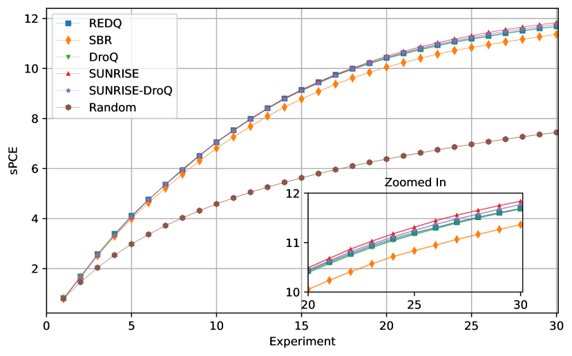
Figure 1: Cumulative sPCE for $K=2$ objects estimated using $L=1e6$. Points are mean sPCE values, and the thickness of the shaded regions at each point are standard errors, all from 20000 rollouts, spread evenly across 10 agents trained under unique random seeds. In both Figures 1 and 3, interpolations and shaded regions between experiment points on the curves are not meaningful, and are only present to emphasise the shading for standard errors.

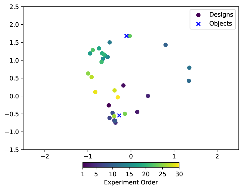
Figure 2: Trained REDQ agent selecting designs at deployment time in the location finding experiment

Observing Figure 1, at deployment time for $K=2$, which is the same setup used during training, the agents all initially start by collecting a similar sPCE value in the first experiment. They follow the same rate, with the first agents to deviate from the pattern being that of an agent randomly choosing designs from the 2nd experiment, and SBR from about the 7th experiment. The random agent ultimately fails to capture the much higher EIG values that the other agents collect. SUNRISE performs best on the same setup used during training, and very well on other numbers of objects.

5.2 Constant Elasticity of Substitution

The constant elasticity of substitution (CES) experiment was explored by Foster et al. (2019), Foster et al. (2020) and Blau et al. (2022). We have two baskets $\boldsymbol{x},\boldsymbol{x^{\prime}}\in[0,100]^{3}$ of goods, and a human indicates their preference of the two baskets on a sliding 0-1 scale. The CES model (Arrow et al. 1961) with latent variables $\boldsymbol{\theta}=(\rho,\boldsymbol{\alpha},u)$, which all characterise the human’s utility for the different items, is then used to measure the difference in utility of the baskets. The goal is to design the baskets in a way that allows for inference of the latent variables. The baskets are 3-tuples, meaning that we have $6$ design space dimensions $(\xi=(\boldsymbol{x},\boldsymbol{x^{\prime}}))$. Hyperparameter details can be found in Appendix C, and experiment details can be found in Appendix D.2.

Table 2 explains the sPCE and sNMC values across two different experimental setups, which vary according to a parameter $\nu$ in the statistical model. Here, the likelihood function used in training differs from that found at deployment time. The training and test distributions are therefore different when $\nu$ is changed, which is a common scenario in the real-world. The agents are trained to maximise sPCE in $T=10$ experiments for $\nu=0.005$. To generalise to an unseen statistical model, an agent should still be able to make maximally informative design choices for the two baskets.

DroQ achieves the best performance on both $\nu=0.005$ and $\nu=0.01$, noting its ability to generalise and sacrifice short-term gains for long-term ones, which we find in Figure 3. SUNRISE performs very well in the location finding experiment, but here it lags behind DroQ. REDQ presents greater sPCE for $\nu=0.005$ than SUNRISE, and so it is possible that because SUNRISE only uses a single Q-function per agent, it does not tackle overestimation bias (Fujimoto, Hoof, and Meger 2018) in the CES experiment very well. For SUNRISE, there could be better alternatives to randomly switching between multiple agents during experimentation; see Appendix F. The difference between REDQ and DroQ is the use of dropout regularisation for the Q-function neural network, which seems to affect performance greatly here. We find that REDQ offers the cheapest training times by about 4 hours compared to DroQ. We also note that DroQ offers larger standard errors for sNMC, compared to the other algorithms. This is not of great concern here, since the estimated sPCE values from DroQ are 2 orders of magnitude larger than the corresponding standard errors, and the $95\%$ confidence intervals – based on the standard errors and centred on the DroQ sNMC estimates – do not overlap with the analogous confidence intervals from the other algorithms. However, when computing DroQ estimates of sNMC in other applications, it would be prudent to monitor for unacceptably large standard errors.

Combining SUNRISE and DroQ does not lead to improved performance over DroQ, but there is an improvement over every other algorithm in terms of sPCE. This is due to using dropout Q-functions in the ensemble. The combination requires much more training time.

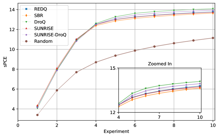
Figure 3: Cumulative sPCE for $\nu=0.005$ estimated using $L=1e7$.

6 Discussion

We investigated five RL algorithms in an effort to produce agents that perform well when the distribution of experimental observations differs from the distribution that the agents were trained under. We examined REDQ, DroQ, SBR, SUNRISE, and SUNRISE-DroQ, finding the best generalisation from DroQ and SUNRISE, depending on the experimental design problem. REDQ can be viewed as a cheap algorithm for obtaining informative experiments, but it loses out to the greater information gain acquired by more computationally expensive algorithms. A scientist should determine the available computational resources for training, before making a judgement on the algorithm they wish to employ.

Overall, the results suggest the SUNRISE-DroQ combination is a good choice for training agents (on possibly misspecified models) that are expected to achieve high information gain in sequential experiments. The combination does come with added expense determined by ensemble size and other algorithm hyperparameters.

These results are indicative, as they suggest which of these algorithms give the best performance on these experimental design problems. However, a number of questions remain. How close to optimal are the policies learnt and what factors strongly influence which policies are (not) learnt? For example, in the location finding experiment, the different RL algorithms appear to converge on similar policies; policies that tend to initially choose designs close to the centre of the experiments’ square-shaped domain. Are such policies close to optimal, and/or are they suggestive of the influence of the radial symmetry in the standard Gaussian prior distribution of the unknown locations? The policy might also be influenced by the radial symmetry in the standard Gaussian distribution of the initial placement of objects at unknown locations. If, instead, training used uninformative, high-entropy distributions (e.g. uniform distributions), this might result in learnt policies that perform better across a wider range of location finding problems. On the other hand, the results might confirm that radial symmetry in initial design choices is necessary for optimal information gain in location finding.

Table 1 suggests that the algorithm with the best performing agents (on $K=2$ experiments) is not necessarily producing agents that are the best under distribution drift (on $K\neq 2$ experiments). The results also suggest there are experimental design problems where a validated, highly performant agent can be expected to remain highly performant under distribution drift. Gaining a good understanding of why, and when, this is the case, is important for applying these algorithms in practice. The SUNRISE and (more expensive) SUNRISE-DroQ algorithms exemplify these observations.

Figures 1 and 3 show larger jumps in cumulative sPCE from earlier experiments, compared to jumps from latter experiments. Are the policies myopically gathering as much information as possible early on, or are the averages obfuscating more sophisticated design choice strategies? There is some subtle evidence in Figure 3 that the DroQ agents might be gathering less information than the other RL agents initially, but eventually DroQ starts dominating them later.

Scientists may be able to afford to conduct additional experiments at deployment time. So, seeing how the RL agents perform over longer horizons would be worth investigating.

For the CES experiment, agents initially appear to maximise sPCE a lot faster than the agents in the location finding experiment (compare Figures 1 and 3). However, the CES experiment agents appear to converge much more slowly to the sPCE theoretical maximum for the CES experiment, $\log(1e7+1)$, compared to the analogous convergence for the location finding agents to $\log(1e6+1)$. This is likely to be an exploration problem, given the small budget. Future work could investigate how certain likelihood function parameters, for both experimental design problems, affect the final sPCE obtained by the agents. Another study could look at the performance of these algorithms on higher dimensional scenarios; e.g. 3-dimensional location finding experiments. One could also craft utility functions that can better address model misspecification and lead to more robust experimental design (Go and Isaac 2022; Catanach and Das 2023).

To conclude, our results showcase an important step towards generalisable RL agents for BOED. We extend the work of Blau et al. (2022) by considering alternative RL algorithms, in aid of constructing generalisable policies.

Appendix A Neural Network Architecture and the HiP-MDP

We explain how the design neural networks are constructed in our experiments and how this relates to our HiP-MDP formulation.

A.1 Neural Network Architecture

The optimal policy is given by $\pi^{*}=\operatorname*{arg\,max}\limits_{\pi}\text{sPCE}(\pi,L,T)$, which maximises the sPCE lower-bound. Recall that sPCE is bounded by $\log(L+1)$, and so the optimal policy should achieve this (as a reward) by the end of experimentation. The approach by Foster et al. (2021), which they coin deep adaptive design (DAD), seeks to approximate the optimal policy $\pi^{*}$ through a neural network, otherwise known as the design network $\pi_{\phi}$. This is then a policy-based approach to sequential BOED, since we now learn and use a policy $\pi$ to select designs, rather than optimising designs at the same time during experimentation. This policy would be learnt offline using the model provided of the Bayesian experimental design problem, and would then be deployed in the online setting for rapid live experiments.

We say that DAD amortises the cost of conducting experiments in experimental design, since we are now learning the parameters $\phi$ of a neural network $\pi_{\phi}$, rather than optimising designs directly during training. This approach eliminates the adaptation costs during the live experiment, as the design network can instantly select the next design with a single forward-pass through the neural network.

In DAD, the neural network architecture for $\pi_{\phi}$ is constructed to allow for permutation invariance, enhancing the efficiency of learning by allowing for weight sharing (Foster et al. 2021). Using the fact that EIG is unchanged under permutation (Foster et al. 2021), we represent the history $h_{t}$ with a fixed-dimensional representation by pooling representations of the distinct design-observation pairs of the history,

$$B_{\psi,t}=\sum_{k=1}^{t}\text{Encoder}_{\psi}(\xi_{k},y_{k}),$$

where $\text{Encoder}_{\psi}$ is a neural network encoder with parameters $\psi$ to be learnt. This pooled representation remains unchanged if we reorder the labels $1,\ldots,t$.

We then construct our design network to make decisions based on the pooled representation $B_{\psi,t}$ by setting,

$$\pi_{\phi}(h_{t})=\text{Emitter}_{\eta}(B_{\psi,t}),$$

where $\text{Emitter}_{\eta}$ is a learnt emitter network. The trainable parameters are $\phi=\{\psi,\eta\}$. By combining simple networks in a way that respects the permutation invariance of the problem, we enable parameter sharing (Foster et al. 2021). This allows the network $\text{Encoder}_{\psi}$ to be reused for each input pair and for each timestep $t$.

The exact architecture of our design network, including the number of nodes and hidden layers, that we use in our results is provided in Appendix C.1.

A.2 HiP-MDP

Blau et al. (2022) explain that each state $s_{t}$ in the state space $\mathcal{S}$ has the form $s_{t}=(B_{\psi,t},C_{t},y_{t})$, where

$$B_{\psi,t}=\sum_{k=1}^{t}\text{Encoder}_{\psi}(\xi_{k},y_{k}),\hskip 4.30554ptC_{t}=\left[\prod_{k=1}^{t}p(y_{k}\mid\boldsymbol{\theta}_{\ell},\xi_{k})\right]^{L}_{\ell=0},$$

and $\text{Encoder}_{\psi}$ is our encoder in the design network with parameters $\psi$, all as explained in Appendix A.1.

This summary of the history (or history summary) follows the Markov property because we can decompose this as

$$B_{\psi,t}=B_{\psi,t-1}+\text{Encoder}_{\psi}(\xi_{t},y_{t}).$$

In other words, we do not need the whole history $h_{t}=(\xi_{1:t},y_{1:t})$ to compute the next summary $B_{\psi,t+1}$. It is then sensible to use $B_{\psi,t}$ as an input for the policy, or in other words, construct a pooled representation of the history $h_{t}$, following the Markovian representation above, and pass this through an emitter network (see Appendix A.1) to obtain the next design to select. The initial state becomes $s_{0}=(\boldsymbol{0},\boldsymbol{1},\emptyset)$. The transition dynamics for $B_{\psi,t}$ follow the Markovian representation above.

Recall that sPCE requires $L$ contrastive samples, being different realisations of the parameter of interest $\boldsymbol{\theta}$. We can compute the sPCE for experiment $t$ as $r_{t}=\mathcal{R}(s_{t-1},a_{t-1},s_{t};\boldsymbol{\theta}_{0:L})$, where

$$\mathcal{R}(s_{t-1},a_{t-1},s_{t};\boldsymbol{\theta}_{0:L})=\log p(y_{t}\mid\boldsymbol{\theta}_{0},\xi_{t})-\log(C_{t}\cdot\boldsymbol{1})+\log(C_{t-1}\cdot\boldsymbol{1}).$$

$C_{t}$ here is a vector of history likelihoods, where each element $c_{t,l}$ is the likelihood of observing the history $h_{t}$ for true parameters $\boldsymbol{\theta}_{l}$. $\boldsymbol{0}$ and $\boldsymbol{1}$ are vectors of zeroes and ones respectively, having the same length as $C_{t}$ or $C_{t+1}$ where sensible. This reward is generally non-zero for each timestep, and there is no need to save the entire history in memory to compute the reward (Blau et al. 2022). Retaining the history likelihood $C_{t}$ and experimental outcome $y_{t}$ is sufficient.

Using the above, Blau et al. (2022) prove that the expected return of the HiP-MDP is equivalent to sPCE using $\gamma=1$. The proof is omitted here, but can be found in Appendix A.2 by Blau et al. (2022).

Appendix B Algorithms

In this appendix, we cover our chosen RL algorithms in more detail, with their respective pseudocode.

B.1 Soft Actor-Critic

It is first sensible to cover the foundational algorithm that our explored variants are based on, the SAC algorithm (Haarnoja et al. 2019).

SAC is an off-policy RL algorithm designed to optimise a stochastic policy in an environment, balancing exploration and exploitation (Haarnoja et al. 2019). SAC aims to maximise both the expected reward and the entropy of the policy. Higher entropy encourages exploration by promoting more stochastic policies, preventing premature convergence to suboptimal policies. This is important in experimental design, as we need to adequately explore the design space to find the appropriate designs that maximise EIG.

SAC follows from maximum-entropy RL (Eysenbach and Levine 2022), with the following objective

$$\pi^{*}=\operatorname*{arg\,max}\limits_{\pi}\sum_{t}\mathbb{E}_{(s_{t},a_{t})\sim\rho_{\pi}}\left[r_{t}+\alpha H(\pi(\cdot\mid s_{t}))\right],$$

where $\alpha$ is the temperature parameter controlling the importance of the entropy term, and $H$ is the entropy term. A higher $\alpha$ value encourages more exploration by making the policy more random, whilst a lower $\alpha$ value leads to more exploitation by making the policy more deterministic.

Haarnoja et al. (2019) derive soft policy iteration, which learns optimal maximum-entropy policies by alternating between policy evaluation and policy improvement in the maximum-entropy framework. This is based on the tabular setting, and so it is expensive to utilise on continuous settings. This brings us to SAC, which uses neural networks to approximate the soft Q-function $Q_{\theta}$ and the policy $\pi_{\phi}$, with parameters $\theta$ and $\phi$ respectively, and optimises them using stochastic gradient descent.

The soft Q-function is updated by minimising the soft Bellman residual, using samples from a replay buffer $D$ and a target soft Q-function with parameters $\theta_{\text{targ}}$,

$$J_{Q}(\theta)=\mathbb{E}_{(s_{t},a_{t})\sim D}\left[\frac{1}{2}\left(Q_{\theta}(s_{t},a_{t})-\left(r_{t}+\gamma\mathbb{E}_{s_{t+1}\sim\mathcal{T}}[\overline{V}_{\theta_{\text{targ}}}(s_{t+1})]\right)\right)^{2}\right],$$

where $\overline{V}_{\chi}(s_{t})=\mathbb{E}_{a_{t}\sim\pi}[Q_{\chi}(s_{t},a_{t})-\alpha\log\pi(a_{t}\mid s_{t})]$ for a Q-function with parameters $\chi$.

The policy is updated by minimising the expected KL-divergence,

$$J_{\pi}(s_{t},\phi)=\mathbb{E}_{s_{t}\sim D}\left[\mathbb{E}_{a_{t}\sim\pi_{\phi}}[\alpha\log\pi_{\phi}(a_{t}\mid s_{t})-Q_{\theta}(s_{t},a_{t})]\right],$$

where the policy is reparameterised using a neural network transformation, by setting $a_{t}=f_{\phi}(\epsilon_{t};s_{t})$ for an input noise vector $\epsilon_{t}$.

Additionally, the temperature parameter can be automatically adjusted to control the entropy term,

$$J(\alpha)=\mathbb{E}_{a_{t}\sim\pi_{t}}[-\alpha\log\pi_{t}(a_{t}\mid s_{t})-\alpha H].$$

By treating the entropy as a constraint, we avoid needing to manually set the often difficult to optimise temperature. The idea here is that the policy should explore regions where the optimal action is uncertain, and become deterministic in regions where the optimal action is clear. $J(\alpha)$ ensures that the average entropy of the policy is constrained, whilst the entropy at different states vary. The temperature eventually decays close to zero during training, making the policy close to fully deterministic.

Full algorithm and gradient details are provided by Haarnoja et al. (2019). We note that SAC employs 2 Q-functions to tackle overestimation bias (Fujimoto, Hoof, and Meger 2018). The SAC parameter updates explained in the pseudocode below are done similarly for the algorithms that follow this subsection.

Algorithm 1 Soft Actor-Critic

1: Initialise policy parameters $\phi$, Q-function parameters $\theta_{1},\theta_{2}$, and empty replay buffer $D$. Set target parameters $\theta_{\text{targ},1}\leftarrow\theta_{1}$, $\theta_{\text{targ},2}\leftarrow\theta_{2}$.

2: for each episode do

3:  Take one action $a_{t}\sim\pi_{\phi}(\cdot\mid s_{t})$. Observe reward $r_{t}$, new state $s_{t+1}$.

4:  Add data to buffer: $D\leftarrow D\cup\{(s_{t},a_{t},r_{t},s_{t+1})\}$

5:  for each gradient step do

6:   Sample a mini-batch $B=\{(s_{t},a_{t},r_{t},s_{t+1})\}$ from $D$

7:   Compute the Q-target $y$ for the Q-functions by

$$y=r_{t}+\gamma\left(\min_{i=1,2}Q_{\theta_{\text{targ},i}}(s_{t+1},\tilde{a}_{t+1})-\alpha\log\pi_{\phi}(\tilde{a}_{t+1}\mid s_{t+1})\right),\quad\tilde{a}_{t+1}\sim\pi_{\phi}(\cdot\mid s_{t+1})$$

8:   for $i=1,2$ do

9:    # Perform the following update below $\theta_{i}\leftarrow\theta_{i}-\lambda_{Q}\nabla_{\theta_{i}}\hat{J}_{Q}(\theta_{i})$

10:    Update $\theta_{i}$ with gradient descent using

$$\nabla_{\theta_{i}}\frac{1}{|B|}\sum_{(s_{t},a_{t},r_{t},s_{t+1})\in B}\left(Q_{\theta_{i}}(s_{t},a_{t})-y\right)^{2}$$

11:    Update target networks with $\theta_{\text{targ},i}\leftarrow\tau\theta_{i}+(1-\tau)\theta_{\text{targ},i}$

12:   end for

13:   # Perform the following update below $\phi\leftarrow\phi-\lambda_{\pi}\nabla_{\phi}\hat{J}_{\pi}(\phi)$

14:   Update policy parameters $\phi$ with gradient ascent using

$$\nabla_{\phi}\frac{1}{|B|}\sum_{s_{t}\in B}\left(\min_{i=1,2}Q_{\theta_{i}}(s_{t},\tilde{a}_{\phi}(s_{t}))-\alpha\log\pi_{\phi}(\tilde{a}_{\phi}(s_{t})\mid s_{t})\right),\quad\tilde{a}_{\phi}(s_{t})\sim\pi_{\phi}(\cdot\mid s_{t})$$

15:   # Perform the following update below $\alpha\leftarrow\alpha-\lambda\nabla_{\alpha}\hat{J}(\alpha)$

16:   Update temperature parameter $\alpha$ by

$$\nabla_{\alpha}\frac{1}{|B|}\sum_{s_{t}\in B}\left(-\alpha\log\pi_{\phi}(\tilde{a}_{\phi}(s_{t})\mid s_{t})-\alpha H\right)$$

17:  end for

18: end for

B.2 Randomised Ensembled Double Q-Learning

REDQ extends SAC through employing various adjustments. This includes a higher UTD ratio (by allowing for $G$ updates as in the algorithm below), the use of an ensemble of Q-functions, and in-target minimisation over a random subset $M$ of the $N$ Q-functions (Chen et al. 2021).

Here, we can use $M$ Q-functions when computing the Q-target, which makes use of our ensemble of $N$ Q-functions. We could set $M=N$ as in SAC, although here we have the advantage of a large ensemble of Q-functions instead of always having 2 Q-functions. Using a small value of $M$, such as $M=2$, has been found to work well (Chen et al. 2021). Following from the SAC algorithm presented above, our Q-target is computed by,

$$y=r_{t}+\gamma\left(\min_{i\in\mathcal{M}}Q_{\theta_{\text{targ},i}}(s_{t+1},\tilde{a}_{t+1})-\alpha\log\pi_{\phi}(\tilde{a}_{t+1}\mid s_{t+1})\right),\quad\tilde{a}_{t+1}\sim\pi_{\phi}(\cdot\mid s_{t+1}),$$

where $\mathcal{M}$ is a (random) set of indices of size $M$ for the ensemble of Q-functions. The difference here from SAC is taking $\min_{i\in\mathcal{M}}$ over the Q-target functions instead of $\min_{i=1,2}$.

Chen et al. (2021) find that REDQ maintains stable and near-uniform bias under high UTD ratios due to its ensemble and in-target minimisation components. Blau et al. (2022) likely use REDQ for this reason. Where Chen et al. (2021) recommend using 10 Q-functions, Blau et al. (2022) instead use 2 Q-functions as in SAC. We assume this choice is due to the computational costs of using a larger ensemble of 10 Q-functions, which we confirm through our empirical tests.

Algorithm 2 Randomised Ensembled Double Q-learning

1: Initialise policy parameters $\phi$, $N$ Q-function parameters $\theta_{i}$, and empty replay buffer $D$. Set target parameters $\theta_{\text{targ},i}\leftarrow\theta_{i}$. All for $i=1,\ldots,N$.

2: for each episode do

3:  Take one action $a_{t}\sim\pi_{\phi}(\cdot\mid s_{t})$. Observe reward $r_{t}$, new state $s_{t+1}$.

4:  Add data to buffer: $D\leftarrow D\cup\{(s_{t},a_{t},r_{t},s_{t+1})\}$

5:  for $G$ updates do

6:   Sample a mini-batch $B=\{(s_{t},a_{t},r_{t},s_{t+1})\}$ from $D$

7:   Sample a set $\mathcal{M}$ of $M$ distinct indices from $\{1,2,\ldots,N\}$

8:   Compute the Q-target $y$ (same for all of the $N$ Q-functions) by

$$y=r_{t}+\gamma\left(\min_{i\in\mathcal{M}}Q_{\theta_{\text{targ},i}}(s_{t+1},\tilde{a}_{t+1})-\alpha\log\pi_{\phi}(\tilde{a}_{t+1}\mid s_{t+1})\right),\quad\tilde{a}_{t+1}\sim\pi_{\phi}(\cdot\mid s_{t+1})$$

9:   for $i=1,\ldots,N$ do

10:    Update $\theta_{i}$ with gradient descent using

$$\nabla_{\theta_{i}}\frac{1}{|B|}\sum_{(s_{t},a_{t},r_{t},s_{t+1})\in B}\left(Q_{\theta_{i}}(s_{t},a_{t})-y\right)^{2}$$

11:    Update target networks with $\theta_{\text{targ},i}\leftarrow\tau\theta_{i}+(1-\tau)\theta_{\text{targ},i}$

12:   end for

13:   Update policy parameters $\phi$ with gradient ascent using

$$\nabla_{\phi}\frac{1}{|B|}\sum_{s_{t}\in B}\left(\frac{1}{N}\sum_{i=1}^{N}Q_{\theta_{i}}(s_{t},\tilde{a}_{\phi}(s_{t}))-\alpha\log\pi_{\phi}(\tilde{a}_{\phi}(s_{t})\mid s_{t})\right),\quad\tilde{a}_{\phi}(s_{t})\sim\pi_{\phi}(\cdot\mid s_{t})$$

14:   Update temperature parameter $\alpha$ by

$$\nabla_{\alpha}\frac{1}{|B|}\sum_{s_{t}\in B}\left(-\alpha\log\pi_{\phi}(\tilde{a}_{\phi}(s_{t})\mid s_{t})-\alpha H\right)$$

15:  end for

16: end for

B.3 Dropout Q-Functions for Doubly Efficient Reinforcement Learning

DroQ is an algorithm that seeks to improve on the computational costs of REDQ by making use of both dropout regularisation (Hinton et al. 2012) and layer normalisation (Ba, Kiros, and Hinton 2016) in the deep Q-functions. A much smaller ensemble of Q-functions can be used due to the inclusion of dropout, such as $N=2$. The main difference here is the use of dropout Q-functions, which we denote by $Q_{\text{Dr}}$ in the algorithm below. There is no in-target minimisation as in REDQ, so we compute the Q-targets using every Q-function in the ensemble.

Algorithm 3 Dropout Q-Functions for Doubly Efficient Reinforcement Learning

1: Initialise policy parameters $\phi$, $N$ Q-function parameters $\theta_{i}$ and empty replay buffer $D$. Set target parameters $\theta_{\text{targ},i}\leftarrow\theta_{i}$. All for $i=1,\ldots,N$.

2: for each episode do

3:  Take action $a_{t}\sim\pi_{\phi}(\cdot\mid s_{t})$. Observe reward $r_{t}$, next state $s_{t+1}$.

4:  $D\leftarrow D\cup\{(s_{t},a_{t},r_{t},s_{t+1})\}$.

5:  for $G$ updates do

6:   Sample a mini-batch $B=\{(s_{t},a_{t},r_{t},s_{t+1})\}$ from $D$.

7:   Compute the Q-target $y$ for the dropout Q-functions by

$$y=r_{t}+\gamma\left(\min_{i=1,\ldots,N}Q_{\text{Dr},\theta_{\text{targ},i}}(s_{t+1},\tilde{a}_{t+1})-\alpha\log\pi_{\phi}(\tilde{a}_{t+1}\mid s_{t+1})\right),\quad\tilde{a}_{t+1}\sim\pi_{\phi}(\cdot\mid s_{t+1})$$

8:   for $i=1,\ldots,N$ do

9:    Update $\theta_{i}$ with gradient descent using

$$\nabla_{\theta_{i}}\frac{1}{|B|}\sum_{(s_{t},a_{t},r_{t},s_{t+1})\in B}\left(Q_{\text{Dr},\theta_{i}}(s_{t},a_{t})-y\right)^{2}$$

10:    Update target networks with $\theta_{\text{targ},i}\leftarrow\tau\theta_{i}+(1-\tau)\theta_{\text{targ},i}$

11:   end for

12:   Update policy parameters $\phi$ with gradient ascent using

$$\nabla_{\phi}\frac{1}{|B|}\sum_{s_{t}\in B}\left(\frac{1}{N}\sum_{i=1}^{N}Q_{\text{Dr},\theta_{i}}(s_{t},\tilde{a}_{\phi}(s_{t}))-\alpha\log\pi_{\phi}(\tilde{a}_{\phi}(s_{t})\mid s_{t})\right),\quad\tilde{a}_{\phi}(s_{t})\sim\pi_{\phi}(\cdot\mid s_{t})$$

13:   Update temperature parameter $\alpha$ by

$$\nabla_{\alpha}\frac{1}{|B|}\sum_{s_{t}\in B}\left(-\alpha\log\pi_{\phi}(\tilde{a}_{\phi}(s_{t})\mid s_{t})-\alpha H\right)$$

14:  end for

15: end for

B.4 Scaled-by-Resetting

SBR (D’Oro et al. 2022) explores how increasing the replay ratio, the number of times an agent’s parameters are updated per environment interaction, can drastically improve sample efficiency. Essentially, the parameters of the neural networks for the agent are periodically reset, either partially or fully, during training. It is fully reset for SAC (D’Oro et al. 2022), and so we employ the same in our work.

In more detail, the Q-functions and policy networks are reset, meaning that the neural network parameters are back to their untrained state. We only retain the replay buffer, and after a reset, the agent is again trained as normal, this time updating its parameters using the previously gathered experiences stored in the replay buffer. This is close to the offline RL setting, where a dataset of experiences is already made available, though here we are also collecting experiences online at the same time.

Our implementation of SBR is built over REDQ, as seen in the pseudocode below.

Algorithm 4 Scaled-by-Resetting

1: Initialise policy parameters $\phi$, $N$ Q-function parameters $\theta_{i}$, and empty replay buffer $D$. Set target parameters $\theta_{\text{targ},i}\leftarrow\theta_{i}$. All for $i=1,\ldots,N$. Set fixed reset interval $\psi$.

2: for each episode do

3:  Take one action $a_{t}\sim\pi_{\phi}(\cdot\mid s_{t})$. Observe reward $r_{t}$, new state $s_{t+1}$.

4:  Add data to buffer: $D\leftarrow D\cup\{(s_{t},a_{t},r_{t},s_{t+1})\}$

5:  for $G$ updates do

6:   Sample a mini-batch $B=\{(s_{t},a_{t},r_{t},s_{t+1})\}$ from $D$

7:   Sample a set $\mathcal{M}$ of $M$ distinct indices from $\{1,2,\ldots,N\}$

8:   Compute the Q-target $y$ (same for all of the $N$ Q-functions) by

$$y=r_{t}+\gamma\left(\min_{i\in\mathcal{M}}Q_{\theta_{\text{targ},i}}(s_{t+1},\tilde{a}_{t+1})-\alpha\log\pi_{\phi}(\tilde{a}_{t+1}\mid s_{t+1})\right),\quad\tilde{a}_{t+1}\sim\pi_{\phi}(\cdot\mid s_{t+1})$$

9:   for $i=1,\ldots,N$ do

10:    Update $\theta_{i}$ with gradient descent using

$$\nabla_{\theta_{i}}\frac{1}{|B|}\sum_{(s_{t},a_{t},r_{t},s_{t+1})\in B}\left(Q_{\theta_{i}}(s_{t},a_{t})-y\right)^{2}$$

11:    Update target networks with $\theta_{\text{targ},i}\leftarrow\tau\theta_{i}+(1-\tau)\theta_{\text{targ},i}$

12:   end for

13:   Update policy parameters $\phi$ with gradient ascent using

$$\nabla_{\phi}\frac{1}{|B|}\sum_{s_{t}\in B}\left(\frac{1}{N}\sum_{i=1}^{N}Q_{\theta_{i}}(s_{t},\tilde{a}_{\phi}(s_{t}))-\alpha\log\pi_{\phi}(\tilde{a}_{\phi}(s_{t})\mid s_{t})\right),\quad\tilde{a}_{\phi}(s_{t})\sim\pi_{\phi}(\cdot\mid s_{t})$$

14:   Update temperature parameter $\alpha$ by

$$\nabla_{\alpha}\frac{1}{|B|}\sum_{s_{t}\in B}\left(-\alpha\log\pi_{\phi}(\tilde{a}_{\phi}(s_{t})\mid s_{t})-\alpha H\right)$$

15:   if number of gradient steps exceeds $\psi$ then

16:    Reset $\phi$, $\theta_{i},\ldots\theta_{N}$, $\theta_{\text{targ},1},\ldots,\theta_{\text{targ},N}$ as done initially, keeping the replay buffer

17:    $\psi\leftarrow\psi+\psi$

18:   end if

19:  end for

20: end for

B.5 Simple Unified Framework for Reinforcement Learning Using Ensembles

SUNRISE is a method designed to enhance off-policy RL algorithms by addressing common challenges like instability in Q-learning (Lee et al. 2021). It achieves this by integrating ensemble-based weighted Bellman backups, which re-weight target Q-values based on uncertainty estimates from a Q-ensemble, and a UCB exploration strategy that selects actions with the highest UCB to encourage efficient exploration.

We explain the UCB exploration strategy (Chen et al. 2017; Lee et al. 2021) in full, which is an important component of our policy ensemble-based algorithm. The UCB exploration formula used in the SUNRISE framework (Lee et al. 2021) is designed to balance exploration and exploitation through using the $N$ candidate actions generated by our $N$ policies. The UCB formula is as follows,

$$a_{t}=\operatorname*{arg\,max}\limits_{a}\{Q_{\text{mean}}(s_{t},a)+\lambda Q_{\text{std}}(s_{t},a)\}.$$

In this formula, $a_{t}$ is the action selected at timestep $t$, which maximises the sum of the mean and a scaled standard deviation of the Q-values. $Q_{\text{mean}}(s_{t},a)$ represents the average estimated value of taking action $a$ in state $s_{t}$, derived from an ensemble of Q-functions. $Q_{\text{std}}(s_{t},a)$ denotes the uncertainty or variance in these Q-value estimates. $\lambda$ controls the weight of the uncertainty term, thus modulating the level of exploration.

Consider an ensemble of $N$ SAC agents, $\{Q_{\theta_{i}},\pi_{\phi_{i}}\}_{i=1}^{N}$, where $\theta_{i}$ and $\phi_{i}$ denote the parameters of the $i$-th soft Q-function and policy, respectively. Conventional Q-learning is based on the Bellman backup, and so it can be affected by error propagation. This essentially means that errors in the previous Q-function induce “noise” to the true Q-value of the current Q-function. Therefore, for each agent $i$, a weighted Bellman backup (Lee et al. 2021) is used instead of $J_{Q}$ from SAC (Haarnoja et al. 2019), given by,

$$J_{WQ}(\tau_{t},\theta_{i})=w(s_{t+1},a_{t+1})\left(Q_{\theta_{i}}(s_{t},a_{t})-r_{t}-\gamma\overline{V}_{\theta_{\text{targ},i}}(s_{t+1})\right)^{2},$$

where $\tau_{t}=(s_{t},a_{t},r_{t},s_{t+1})$ is a transition, $a_{t+1}\sim\pi_{\phi_{i}}(a_{t}\mid s_{t})$, $\overline{V}$ is the value function, defined as in SAC, and $w(s_{t},a_{t})$ is a confidence weight based on an ensemble of target Q-functions.

The confidence weight $w(s_{t},a_{t})$ (Lee et al. 2021) is defined as,

$$w(s_{t},a_{t})=\sigma\left(-\overline{Q}_{\text{std}}(s_{t},a_{t})\cdot\delta\right)+0.5,$$

where $\delta>0$ is a temperature, $\sigma$ is the sigmoid function, and $\overline{Q}_{\text{std}}(s_{t},a_{t})$ is the empirical standard deviation of all target Q-functions $\{Q_{\theta_{\text{targ},i}}\}_{i=1}^{N}$.

Algorithm 5 Simple Unified Framework for Reinforcement Learning Using Ensembles

1: Initialise $N$ policy parameters $\phi_{i}$, $N$ Q-function parameters $\theta_{i}$, and empty replay buffer $D$. Set target parameters $\theta_{\text{targ},i}\leftarrow\theta_{i}$ and initial temperature parameters $\alpha_{i}$. All for $i=1,\ldots,N$.

2: for each episode do

3:  for each timestep $t$ do

4:   Collect $N$ action samples: $A_{t}=\{a_{t,i}\sim\pi_{\phi_{i}}(a\mid s_{t})\mid i\in\{1,\ldots,N\}\}$

5:   Choose the action that maximises UCB by

$$a_{t}=\operatorname*{arg\,max}\limits_{a_{t,i}\in A_{t}}\left(Q_{\text{mean}}(s_{t},a_{t,i})+\lambda Q_{\text{std}}(s_{t},a_{t,i})\right)$$

6:   Collect state $s_{t+1}$ and reward $r_{t}$ from the environment by taking action $a_{t}$

7:   Sample bootstrap masks $M_{t}=\{m_{t,i}\sim\text{Bernoulli}(\beta)\mid i\in\{1,\ldots,N\}\}$

8:   Store transitions $\tau_{t}=(s_{t},a_{t},s_{t+1},r_{t})$ and masks in replay buffer $D\leftarrow D\cup\{(\tau_{t},M_{t})\}$

9:  end for

10:  for $G$ updates do

11:   Sample random minibatch $\{(\tau_{j},M_{j})\}_{j=1}^{B}\sim D$

12:   for each agent $i$ do

13:    # $J_{WQ}$ as found above

14:    Update the Q-function by minimising

$$\nabla_{\theta_{i}}\frac{1}{|B|}\sum_{j=1}^{B}m_{j,i}\cdot J_{WQ}(\tau_{j},\theta_{i})$$

15:    Update target networks with $\theta_{\text{targ},i}\leftarrow\tau\theta_{i}+(1-\tau)\theta_{\text{targ},i}$

16:    # $J_{\pi}$ as found in SAC

17:    Update the policy by minimising

$$\nabla_{\phi_{i}}\frac{1}{|B|}\sum_{j=1}^{B}m_{j,i}\cdot J_{\pi}(s_{j},\phi_{i})$$

18:    # $J(\alpha)$ as found in SAC

19:    Update temperature parameter by minimising

$$\nabla_{\alpha_{i}}\frac{1}{|B|}\sum_{j=1}^{B}m_{j,i}\cdot J(\alpha_{i})$$

20:   end for

21:  end for

22: end for

Our implementation of SUNRISE slightly differs from the default algorithm above, where the only difference is that we do not sample any bootstrap masks, which is simply the equivalent of $\beta=1$ (where the binary masks would all be equal to 1). Lee et al. (2021) find that $\beta=1$ performs the best, making this a sensible adjustment to the algorithm that can also reduce the overall agent training time. See Appendix F for how we decided to deploy our SUNRISE agents at deployment time.

Appendix C Training Regimes

In this section, we explain our training regimes used to obtain our results in more detail. This includes our exact neural network architectures and any hyperparameter optimisation.

C.1 Neural Network, Training, Environment, and Evaluation Details

Neural Networks

In all of our experiments, the (trained) policies are neural networks that consist of an encoder network and an emitter network, as we explain in Appendix A.

Our encoder network, which takes the observation space dimensions as its input, consists of two hidden layers, each with 128 nodes, and the rectified linear unit (ReLU) activation function is used to introduce nonlinearity between the layers. The final pooled representation from the encoder consists of $\frac{128}{2}=64$ nodes, without any activation function. Our emitter network, which takes as input the encoded representation from the encoder, consists of two hidden layers, each with 128 nodes, and the rectified linear unit (ReLU) activation function is used to introduce nonlinearity between the layers. This is evaluated as usual as a TanhNormal policy in SAC (Haarnoja et al. 2019), and we obtain a (stochastic) distribution over the design space as output.

The Q-functions follow the same structure as the policies, and depending on whether dropout and layer normalisation are used, they have the same architecture in every experiment. If dropout and layer normalisation are required, they are deployed before the activation function, starting with dropout. The Q-functions each output a Q-value for all actions.

Training

We use the Adam (Kingma and Ba 2017) optimiser for the policy, the Q-functions, and for controlling $\alpha$ (the exploration parameter) during training. All agents are trained using 20000 iterations. We train with $L=1e5$ contrastive samples for every agent on the sPCE objective. We sample 4096 transitions from the replay buffer for a single optimisation step (mini-batch size). 10 agents are trained under unique random seeds for each algorithm, which we use for our evaluation later.

Environment

In RL, it is possible to normalise/scale the actions, observations, and rewards in the environment (our experimental design problem). Since we want the exact sPCE, we do not perform reward scaling. Actions are scaled to be in range [-1, 1], and observations are scaled to be in range [0, 1].

Evaluation

RL is known to not be very robust to random seeds, so measuring the average performance across agents trained with unique random seeds is a sensible approach to statistically evaluating our algorithms (both during training and at deployment time) (Colas, Sigaud, and Oudeyer 2022). At deployment/evaluation time, we take the average performance of each agent across 2000 rollouts, meaning 2000 different choices of $\boldsymbol{\theta}$ in our Bayesian experimental design problem. Bear in mind that this is for a single agent that has been trained with a particular random seed, and so we do the same for all 10 agents trained with unique random seeds, and take the average performance of this. Since we have 10 agents, our final average performance for each metric would be based on $2000\cdot 10=20000$ different choices of $\boldsymbol{\theta}$ in our experimental design problem. This is a reasonably large number of scenarios to consider, much larger than that by Blau et al. (2022), making our results robust.

C.2 REDQ Hyperparameters

Blau et al. (2022) perform some hyperparameter optimisation on the target update rate $\tau$, policy learning rate, critic (or Q-function) learning rate, replay buffer size, and discount factor $\gamma$. Their best set of hyperparameters are listed in the table below as ‘REDQ’. This is the same set of hyperparameters we used for the results explained in the main body of this paper, for a fair comparison to Blau et al. (2022).

We additionally test on our own accord a discount factor of 0.99 (REDQ-Disc-0.99), ensemble of 10 Q-functions as done by Chen et al. (2021) (REDQ-Ens-10), and a target update rate of 0.01 (REDQ-Tau-0.01).

Parameter	REDQ	REDQ-Disc-0.99	REDQ-Ens-10	REDQ-Tau-0.01
$N$	2	2	10	2
$M$	2	2	2	2
$\gamma$	0.9	0.99	0.9	0.9
$\tau$	0.001	0.001	0.001	0.01
UTD Ratio $G$	64	64	64	64
Policy Learning Rate	0.0001	0.0001	0.0001	0.0001
Critic Learning Rate	0.0003	0.0003	0.0003	0.0003
Buffer Size	10000000	10000000	10000000	10000000

Table 3: REDQ Hyperparameter Combinations

The sPCE and sNMC results at deployment time from using these hyperparameters are explained in the tables below:

	sPCE					Time
	$K=1$	$K=2$	$K=3$	$K=4$	$K=5$	$K=2$
REDQ	$6.279\pm 0.013$	$11.689\pm 0.012$	$11.881\pm 0.013$	$11.507\pm 0.015$	$11.095\pm 0.017$	13.23h
REDQ-Disc-0.99	$6.328\pm 0.012$	$11.536\pm 0.013$	$11.685\pm 0.014$	$11.250\pm 0.015$	$10.825\pm 0.017$	13.41h
REDQ-Ens-10	6.423 $\pm$ 0.013	11.744 $\pm$ 0.013	$11.884\pm 0.013$	$11.419\pm 0.015$	$10.989\pm 0.017$	38.91h
REDQ-Tau-0.01	$6.286\pm 0.013$	$11.651\pm 0.013$	11.919 $\pm$ 0.013	11.516 $\pm$ 0.015	11.177 $\pm$ 0.016	13.38h

Table 4: sPCE at $T=30$ computed using $L=1e6$, and average agent training time for the location finding experiment. Means and standard errors are from 20000 rollouts, spread evenly across 10 agents trained under unique random seeds. The average training time is across these 10 agents.

	sNMC
	$K=1$	$K=2$	$K=3$	$K=4$	$K=5$
REDQ	$6.282\pm 0.013$	$12.323\pm 0.019$	$13.215\pm 0.029$	$12.726\pm 0.030$	$12.190\pm 0.030$
REDQ-Disc-0.99	$6.331\pm 0.012$	$12.071\pm 0.018$	$12.704\pm 0.025$	$12.170\pm 0.027$	$11.653\pm 0.028$
REDQ-Ens-10	6.425 $\pm$ 0.013	12.427 $\pm$ 0.019	$13.140\pm 0.028$	$12.513\pm 0.029$	$11.943\pm 0.029$
REDQ-Tau-0.01	$6.289\pm 0.013$	$12.270\pm 0.019$	13.261 $\pm$ 0.028	12.755 $\pm$ 0.030	12.332 $\pm$ 0.031

Table 5: sNMC at $T=30$ computed using $L=1e6$ for the location finding experiment. Means and standard errors are from 20000 rollouts, spread evenly across 10 agents trained under unique random seeds.

For the location finding experiment, REDQ-Ens-10 is the most expensive to train, and only provides the best results for $K\in\{1,2\}$. REDQ-Tau-0.01 provides the best results for $K\geq 3$, in a much cheaper amount of time.

	sPCE		sNMC		Time
	$\nu=0.005$	$\nu=0.01$	$\nu=0.005$	$\nu=0.01$	$\nu=0.005$
REDQ-Blau	13.782 $\pm$ 0.021	$12.343\pm 0.022$	$19.911\pm 0.155$	$13.433\pm 0.046$	8.95h
REDQ-Disc-0.99	$13.723\pm 0.021$	$12.317\pm 0.023$	$20.240\pm 0.164$	$13.494\pm 0.049$	10.69h
REDQ-Ens-10	$13.781\pm 0.021$	$12.304\pm 0.021$	$18.989\pm 0.138$	$13.192\pm 0.042$	24.75h
REDQ-Tau-0.01	$13.763\pm 0.022$	12.413 $\pm$ 0.023	22.116 $\pm$ 0.216	14.034 $\pm$ 0.061	10.67h

Table 6: sPCE and sNMC at $T=10$ computed using $L=1e7$, and average agent training time for the CES experiment. Means and standard errors are from 20000 rollouts, spread evenly across 10 agents trained under unique random seeds. The average training time is across these 10 agents.

For the CES experiment, REDQ-Blau is best in terms of sPCE when evaluated on the same statistical model used during training. It falls behind REDQ-Tau-0.01 when the model is changed. REDQ-Tau-0.01 provides the greatest sNMC values, suggesting that $\tau=0.01$ may be sensible to train agents with.

C.3 DroQ Hyperparameters

Hiraoka et al. (2022) find empirically that smaller dropout rates provide better performance over larger ones. We compare the performance between dropout rates of 0.01 and 0.1. There are no resets for DroQ and so these are left blank in Table 7 below:

Parameter	DroQ-0.01	DroQ-0.1	SBR-300000	SBR-430000
$N$	2	2	2	2
$M$	2	2	2	2
$\gamma$	0.9	0.9	0.9	0.9
$\tau$	0.001	0.001	0.001	0.001
UTD Ratio $G$	64	64	64	64
Dropout Probability	0.01	0.1	-	-
Reset Interval	-	-	300000	430000
Policy Learning Rate	0.0001	0.0001	0.0001	0.0001
Critic Learning Rate	0.0003	0.0003	0.0003	0.0003
Buffer Size	10000000	10000000	10000000	10000000

Table 7: DroQ and SBR Hyperparameter Combinations

For the location finding finding experiment we use 0.01, and for the CES experiment we use 0.1. These are the best hyperparameter combinations as explained in the tables below:

	sPCE					Time
	$K=1$	$K=2$	$K=3$	$K=4$	$K=5$	$K=2$
DroQ-0.01	6.368 $\pm$ 0.013	11.680 $\pm$ 0.013	11.902 $\pm$ 0.013	11.480 $\pm$ 0.015	11.090 $\pm$ 0.017	19.05h
DroQ-0.1	$6.333\pm 0.013$	$11.176\pm 0.013$	$11.708\pm 0.014$	$11.384\pm 0.016$	$11.090\pm 0.017$	19.63h

Table 8: sPCE at $T=30$ computed using $L=1e6$, and average agent training time for the location finding experiment. Means and standard errors are from 20000 rollouts, spread evenly across 10 agents trained under unique random seeds. The average training time is across these 10 agents.

	sNMC
	$K=1$	$K=2$	$K=3$	$K=4$	$K=5$
DroQ-0.01	6.371 $\pm$ 0.013	12.349 $\pm$ 0.020	13.231 $\pm$ 0.028	12.669 $\pm$ 0.029	$12.147\pm 0.030$
DroQ-0.1	$6.336\pm 0.013$	$11.626\pm 0.019$	$12.980\pm 0.029$	$12.594\pm 0.030$	12.232 $\pm$ 0.031

Table 9: sNMC at $T=30$ computed using $L=1e6$ for the location finding experiment. Means and standard errors are from 20000 rollouts, spread evenly across 10 agents trained under unique random seeds.

	sPCE		sNMC		Time
	$\nu=0.005$	$\nu=0.01$	$\nu=0.005$	$\nu=0.01$	$\nu=0.005$
DroQ-0.01	$13.902\pm 0.020$	$12.427\pm 0.021$	$19.904\pm 0.140$	$13.479\pm 0.043$	12.65h
DroQ-0.1	14.090 $\pm$ 0.020	12.683 $\pm$ 0.022	21.764 $\pm$ 0.201	14.108 $\pm$ 0.058	13.18h

Table 10: sPCE and sNMC at $T=10$ computed using $L=1e7$, and average agent training time for the CES experiment. Means and standard errors are from 20000 rollouts, spread evenly across 10 agents trained under unique random seeds. The average training time is across these 10 agents.

Using a dropout rate of 0.01 is clearly more competitive than using a dropout rate of 0.1 for the location finding experiment. This is reversed for the CES experiment.

C.4 SBR Hyperparameters

One hyperparameter set looks at 2 resets of the neural network parameters during training, and the other looks at 4 resets during training. These are represented as reset intervals $x$ in the algorithm, where we perform a reset every $x$ amount of gradient steps. Table 7 displays the SBR hyperparameter combinations. There is no dropout involved, and so these are left blank (or equivalently set to 0).

We use SBR-430000 for both experimental design problems, due to the explained performance provided in the tables below:

	sPCE					Time
	$K=1$	$K=2$	$K=3$	$K=4$	$K=5$	$K=2$
SBR-300000	$6.020\pm 0.012$	$11.178\pm 0.013$	$11.773\pm 0.014$	11.608 $\pm$ 0.015	11.436 $\pm$ 0.016	13.30h
SBR-430000	6.165 $\pm$ 0.012	11.362 $\pm$ 0.013	11.788 $\pm$ 0.014	$11.518\pm 0.016$	$11.257\pm 0.017$	13.52h

Table 11: sPCE at $T=30$ computed using $L=1e6$, and average agent training time for the location finding experiment. Means and standard errors are from 20000 rollouts, spread evenly across 10 agents trained under unique random seeds. The average training time is across these 10 agents.

	sNMC
	$K=1$	$K=2$	$K=3$	$K=4$	$K=5$
SBR-300000	$6.021\pm 0.012$	$11.515\pm 0.016$	$12.960\pm 0.027$	12.991 $\pm$ 0.031	12.826 $\pm$ 0.032
SBR-430000	6.168 $\pm$ 0.013	11.793 $\pm$ 0.017	13.043 $\pm$ 0.028	$12.886\pm 0.032$	$12.571\pm 0.032$

Table 12: sNMC at $T=30$ computed using $L=1e6$ for the location finding experiment. Means and standard errors are from 20000 rollouts, spread evenly across 10 agents trained under unique random seeds.

For the location finding experiment, we do note that the results for $K\geq 4$ suggest that SBR-300000 is better for this setting. SBR-430000 is otherwise the strongest performer for $K<4$, which is the reason why we choose this as our main hyperparameter combination.

	sPCE		sNMC		Time
	$\nu=0.005$	$\nu=0.01$	$\nu=0.005$	$\nu=0.01$	$\nu=0.005$
SBR-300000	$13.047\pm 0.026$	$11.688\pm 0.026$	$18.248\pm 0.134$	$12.586\pm 0.044$	9.02h
SBR-430000	13.640 $\pm$ 0.022	12.241 $\pm$ 0.023	20.567 $\pm$ 0.179	13.519 $\pm$ 0.052	9.03h

Table 13: sPCE and sNMC at $T=10$ computed using $L=1e7$, and average agent training time for the CES experiment. Means and standard errors are from 20000 rollouts, spread evenly across 10 agents trained under unique random seeds. The average training time is across these 10 agents.

SBR-430000 performs best for both sPCE and sNMC on the two statistical models considered.

C.5 SUNRISE Hyperparameters

We perform hyperparameter optimisation on the Bellman temperature $\delta$, rather than on the UCB weight $\lambda$. To avoid heavy computation, we stick to $N=2$ agents, making the algorithm comparable to the others explored. We explore $\delta=10$ (SUNRISE-10) and $\delta=20$ (SUNRISE-20). There is no dropout involved, and so these are left blank (or equivalently set to 0).

Parameter	SUNRISE-10	SUNRISE-20	Ours-Location	Ours-CES
$N$	2	2	2	2
$\gamma$	0.9	0.9	0.9	0.9
$\tau$	0.001	0.001	0.01	0.01
UTD Ratio $G$	64	64	64	64
UCB $\lambda$	1	1	1	1
Dropout Probability	-	-	0.01	0.1
Bellman Temperature $\delta$	10	20	20	10
Policy Learning Rate	0.0001	0.0001	0.0001	0.0001
Critic Learning Rate	0.0003	0.0003	0.0003	0.0003
Buffer Size	10000000	10000000	10000000	10000000

Table 14: SUNRISE and SUNRISE-DroQ Hyperparameter Combinations

We use SUNRISE-20 for the location finding experiment and SUNRISE-10 for the CES experiment, due to the results explained in the tables below:

	sPCE					Time
	$K=1$	$K=2$	$K=3$	$K=4$	$K=5$	$K=2$
SUNRISE-10	6.355 $\pm$ 0.012	$11.782\pm 0.012$	$12.094\pm 0.013$	$11.837\pm 0.014$	$11.407\pm 0.016$	21.17h
SUNRISE-20	$6.340\pm 0.013$	11.837 $\pm$ 0.012	12.133 $\pm$ 0.013	11.846 $\pm$ 0.014	11.445 $\pm$ 0.016	21.44h

Table 15: sPCE at $T=30$ computed using $L=1e6$, and average agent training time for the location finding experiment. Means and standard errors are from 20000 rollouts, spread evenly across 10 agents trained under unique random seeds. The average training time is across these 10 agents.

	sNMC
	$K=1$	$K=2$	$K=3$	$K=4$	$K=5$
SUNRISE-10	6.358 $\pm$ 0.012	$12.477\pm 0.019$	13.662 $\pm$ 0.030	13.397 $\pm$ 0.032	$12.765\pm 0.032$
SUNRISE-20	$6.342\pm 0.013$	12.555 $\pm$ 0.019	$13.656\pm 0.029$	$13.345\pm 0.030$	12.823 $\pm$ 0.032

Table 16: sNMC at $T=30$ computed using $L=1e6$ for the location finding experiment. Means and standard errors are from 20000 rollouts, spread evenly across 10 agents trained under unique random seeds.

SUNRISE-20 performs best for all $K$, bar $K=1$ on the location finding experiment in terms of sPCE. We note that the sNMC values are higher for SUNRISE-10 under certain values of $K$. Since sPCE is our main metric of interest, ensuring that the true EIG is at least equal to or higher than a certain value, we choose to stick with SUNRISE-20.

	sPCE		sNMC		Time
	$\nu=0.005$	$\nu=0.01$	$\nu=0.005$	$\nu=0.01$	$\nu=0.005$
SUNRISE-10	13.725 $\pm$ 0.022	12.381 $\pm$ 0.023	21.429 $\pm$ 0.199	13.812 $\pm$ 0.058	15.11h
SUNRISE-20	$13.633\pm 0.022$	$12.261\pm 0.023$	$19.815\pm 0.130$	$13.344\pm 0.042$	15.20h

Table 17: sPCE and sNMC at $T=10$ computed using $L=1e7$, and average agent training time for the CES experiment. Means and standard errors are from 20000 rollouts, spread evenly across 10 agents trained under unique random seeds. The average training time is across these 10 agents.

For the CES experiment, SUNRISE-10 stands out as the best performer across all evaluated statistical models and metrics.

C.6 SUNRISE with Dropout Q-Functions Hyperparameters

There is no hyperparameter optimisation involved for SUNRISE-DroQ. We use our own intuition for selecting the hyperparameters to train with based on the results from the previous algorithms. Our final chosen hyperparameters are presented in Table 14, where Ours-Location is the set used for the location finding experiment, and Ours-CES is the set used for the CES experiment.

The following tables are for Ours-Location and Ours-CES, respectively (note that the deployment sPCE and sNMC results below are for the same trained agents, so the training time displayed is equal):

						Time
	$K=1$	$K=2$	$K=3$	$K=4$	$K=5$	$K=2$
Ours-sPCE	$6.433\pm 0.012$	$11.770\pm 0.012$	$12.143\pm 0.013$	$11.831\pm 0.014$	$11.453\pm 0.016$	29.77h
Ours-sNMC	$6.436\pm 0.012$	$12.476\pm 0.019$	$13.664\pm 0.028$	$13.340\pm 0.031$	$12.813\pm 0.032$	29.77h

Table 18: sPCE and sNMC at $T=30$ computed using $L=1e6$, and average agent training time for the location finding experiment. Means and standard errors are from 20000 rollouts, spread evenly across 10 agents trained under unique random seeds. The average training time is across these 10 agents.

			Time
	$\nu=0.005$	$\nu=0.01$	$\nu=0.005$
Ours-sPCE	$13.938\pm 0.021$	$12.544\pm 0.022$	18.16h
Ours-sNMC	$21.210\pm 0.165$	$13.875\pm 0.049$	18.16h

Table 19: sPCE and sNMC at $T=10$ computed using $L=1e7$, and average agent training time for the CES experiment. Means and standard errors are from 20000 rollouts, spread evenly across 10 agents trained under unique random seeds. The average training time is across these 10 agents.

Appendix D Experimental Design Problems

This appendix explains the experimental design problems in more detail, including their probabilistic models and parameters used in our experiments.

Our code is adapted from the repository by Blau et al. (2022), which consists of experimental design problems built under the Pyro probabilistic programming language (Bingham et al. 2018). All experimental design problems now allow for generalisability testing.

D.1 Location Finding

There are $K$ objects on a $d$-dimensional space, and in this experiment we need to identify their locations $\boldsymbol{\theta}=\{\boldsymbol{\beta}_{i}\}_{i=1}^{K}$ based on the signals that the objects emit. We select designs $\xi$, which are the coordinates chosen to observe the signal intensity, in an effort to learn the locations of the objects. Our spaces are restricted in $\xi\in[-4,4]^{d}$ to make the problem more tractable. $T=30$ experiments are conducted both during training and during deployment time, which means that agents can only afford to perform 30 experiments to achieve the highest information gain possible.

The total intensity at point $\xi$ is the superposition of the individual intensities for each object,

$$\mu(\boldsymbol{\theta},\xi)=b+\sum_{i=1}^{K}\frac{\alpha}{m+||\boldsymbol{\beta}_{i}-\xi||^{2}},$$

where $\alpha$ is a constant, $b>0$ is a constant controlling the background signal, and $m>0$ is a constant controlling the maximum signal. The total intensity is then used in the likelihood function calculation.

For an object $\boldsymbol{\beta}_{i}\in\mathbb{R}^{d}$, we use a standard normal prior given by

$$\boldsymbol{\beta}_{i}\sim\mathcal{N}_{d}(\boldsymbol{0},I),$$

where $\boldsymbol{0}$ is the mean vector, and $I$ is the covariance matrix, an identity matrix, both with dimension $d$.

The likelihood function is the logarithm of the total signal intensity $\mu(\boldsymbol{\theta},\xi)$ with Gaussian noise $\sigma$. For a given design $\xi$, the likelihood function is given by

$$y\mid\boldsymbol{\theta},\xi\sim\mathcal{N}(\log\mu(\boldsymbol{\theta},\xi),\sigma^{2}).$$

The parameters we used are provided in the table below, and we note that $K$ differs at deployment time for our generalisability tests:

Parameter	Value
$K$	2
$d$	2
$\alpha$	1
$b$	0.1
$m$	0.0001
$\sigma$	0.5

Table 20: Location Finding Parameters

D.2 Constant Elasticity of Substitution

We have two baskets $\boldsymbol{x},\boldsymbol{x^{\prime}}\in[0,100]^{3}$ of goods, and a human indicates their preference of the two baskets on a sliding 0-1 scale. The CES model (Arrow et al. 1961) with latent variables $(\rho,\boldsymbol{\alpha},u)$, which all characterise the human’s utility or preferences for the different items, is then used to measure the difference in utility of the baskets. We select the two baskets $\boldsymbol{x},\boldsymbol{x^{\prime}}$ in a way that allows us to infer the human’s preferences. $T=10$ experiments are conducted both during training and deployment time.

The CES model (Arrow et al. 1961) defines the utility $U(\boldsymbol{x})$ for a basket of goods $\boldsymbol{x}$ as,

$$U(\boldsymbol{x})=\left(\sum_{i}x_{i}^{\rho}\alpha_{i}\right)^{\frac{1}{\rho}},$$

where $\rho$ and $\boldsymbol{\alpha}$ are latent variables defined with the prior distributions explained below. This utility function, which is a measure of satisfaction in economic terms, is then used in the likelihood function calculation.

To formulate our CES experiment in the Bayesian framework, we need to define a prior distribution for each of the latent variables. We follow the lead of Foster et al. (2020) and Blau et al. (2022) by using the following priors for $(\rho,\boldsymbol{\alpha},u)$,

$$\rho \sim\text{Beta}(1,1)$$

$$\boldsymbol{\alpha} \sim\text{Dirichlet}([1,1,1])$$

$$u \sim\text{Log-Normal}(1,3^{2}).$$

The likelihood function is the preference of the human on a sliding 0-1 scale, which is based on $U(\boldsymbol{x})-U(\boldsymbol{x^{\prime}})$. For a given design $\xi$, the likelihood function is given by,

$$\mu_{\eta} =u\cdot(U(\boldsymbol{x})-U(\boldsymbol{x^{\prime}}))$$

$$\sigma_{\eta} =\nu u\cdot(1+\|\boldsymbol{x}-\boldsymbol{x^{\prime}}\|)$$

$$\eta \sim\mathcal{N}(\mu_{\eta},\sigma_{\eta}^{2})$$

$$y =\text{clip}(s(\eta),\epsilon,1-\epsilon),$$

where $\nu=0.005$, $\epsilon=2^{-22}$, and $s(x)=\frac{1}{1+e^{-x}}$ is the sigmoid function. Notice that the normally distributed $\eta$ is passed through the sigmoid function, bounding $\eta\in[0,1]$. Censoring/clipping is applied, which limits the distribution by setting values above $u=1-\epsilon$ to be equal to $1-\epsilon$, and values below $l=\epsilon$ to be equal to $\epsilon$.

The only parameter that changes for our generalisability tests is $\nu$, where we test for $\nu=0.01$ too. Other parameters remain the same during training and deployment.

Appendix E Training Performance Plots

The plots that follow are the training performance of each agent under the hyperparameter combinations explained in Appendix C. They all explain the rewards, or sPCE, that the agents are able to achieve (on average) at a particular point in training. These are averaged across 10 agents trained under unique random seeds, as done in all of the statistics presented in this paper.

E.1 Location Finding

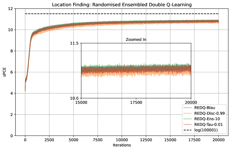
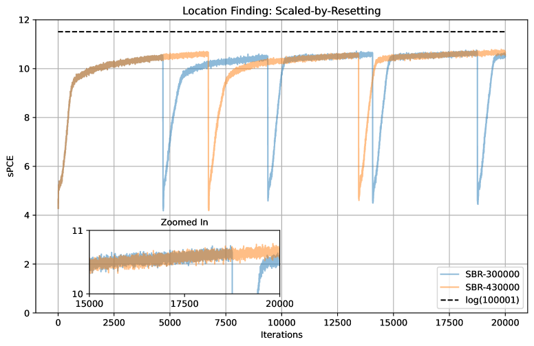
(a) REDQ	(b) DroQ
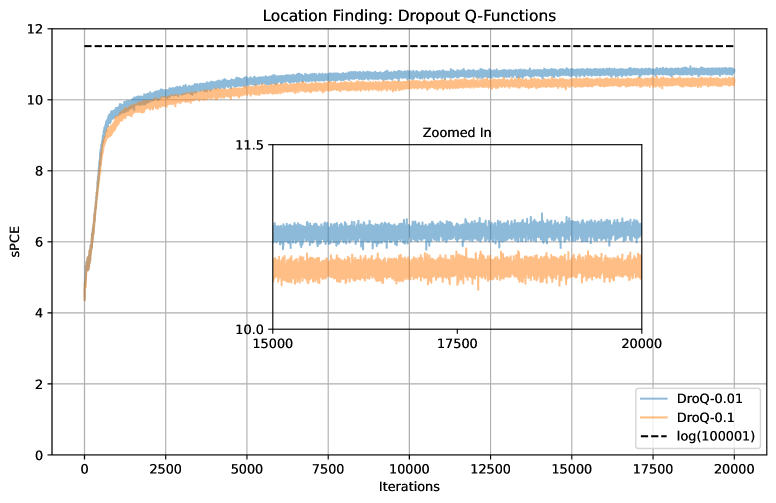
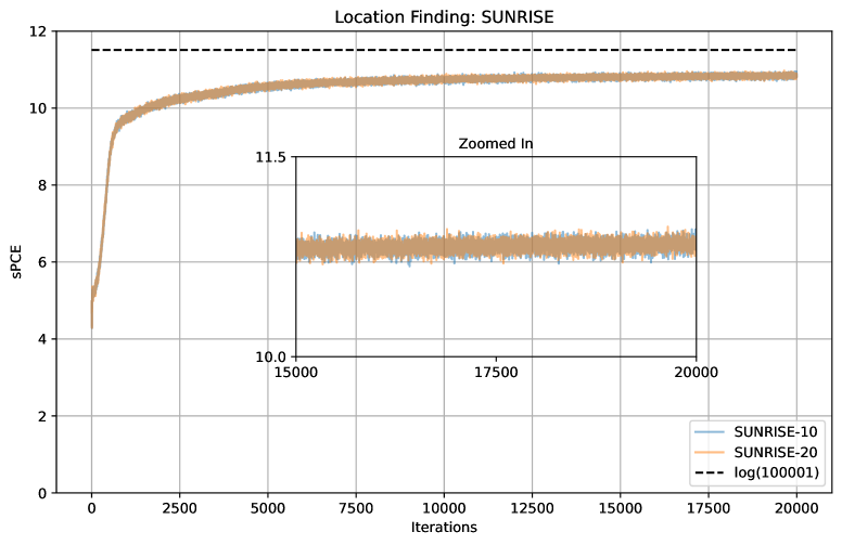
(c) SBR	(d) SUNRISE

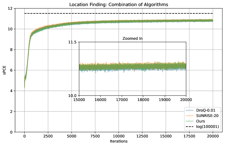
(e) SUNRISE-DroQ

Figure 4: sPCE at $T=30$ training performance, under several hyperparameter combinations and algorithms, for the location finding experiment. sPCE is computed using $L=1e5$, displayed as a dotted line on the plots.

E.2 Constant Elasticity of Substitution

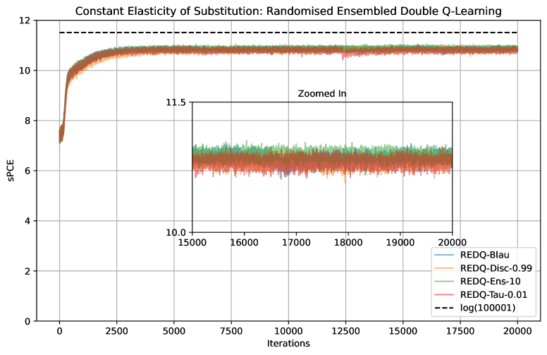
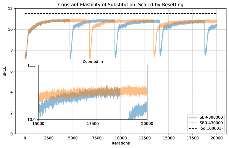
(a) REDQ	(b) DroQ
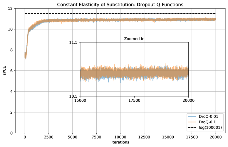
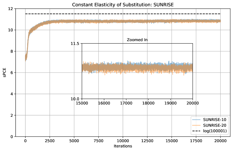
(c) SBR	(d) SUNRISE

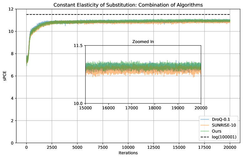
(e) SUNRISE-DroQ

Figure 5: sPCE at $T=10$ training performance, under several hyperparameter combinations and algorithms, for the CES experiment. sPCE is computed using $L=1e5$, displayed as a dotted line on the plots.

Appendix F SUNRISE Tweaks

We explain how we tweaked the SUNRISE algorithm at deployment time, in an effort to offer more informative design choices.

One major change from our SUNRISE implementation and that explored by Lee et al. (2021) is how we use our ensemble of agents at deployment time. Lee et al. (2021) choose to average the means of the TanhNormal distributions modelled by each ensemble policy, and use this average as the next design to select. We empirically find that performance severely falls behind that of the other algorithms through this evaluation method, at least for the location finding experiment. We therefore propose two alternatives to evaluating the agents:

1. Randomly selecting a policy to sample an action from;

2. Forming a new TanhNormal distribution to sample actions from based on the average means and average variances of the ensemble policies. The average of the means is used as the mean, and the average of the variances is used as the variance for the new TanhNormal distribution.

In the results tables displayed for each experimental design problem, SUNRISE-20-A is the agent that follows the evaluation method by Lee et al. (2021) using $\delta=20$. A similar naming convention is used for the other evaluation methods of SUNRISE-20. SUNRISE-20-B are two distinct agents that randomly select a policy to sample an action from at deployment time, our first alternative method. SUNRISE-20-C uses the average means and average variances to formulate a new policy to sample actions from, our second alternative method. The underlying trained agent here is SUNRISE-20. The only change is how we deploy SUNRISE-20 at deployment time through the methods explained.

F.1 Location Finding

We find that the first evaluation method yields superior performance for both sPCE and sNMC, since we are sampling an action from a real distribution learnt during training, and not one that was combined through simply constructing a new distribution based on averaging. Of course, other methods could be explored instead of averaging, or by forming an alternative distribution. The results presented in the main body of this paper, and before this appendix, follow the first evaluation method we propose.

SUNRISE-20-A performs the worst across the board, as we find empirically. We can safely conclude that, at least in our investigated approach, that the evaluation method proposed by Lee et al. (2021) does not offer the impressive results that SUNRISE seeks to deliver. SUNRISE-20-C, while it performs slightly better, also fails to achieve useful values of sPCE. SUNRISE-20-B offers performance comparable to the other algorithms investigated.

	sPCE
	$K=1$	$K=2$	$K=3$	$K=4$	$K=5$
SUNRISE-20-A	$5.947\pm 0.011$	$8.761\pm 0.019$	$8.533\pm 0.020$	$7.972\pm 0.020$	$7.539\pm 0.020$
SUNRISE-20-B	6.340 $\pm$ 0.013	11.837 $\pm$ 0.012	12.133 $\pm$ 0.013	11.846 $\pm$ 0.014	11.445 $\pm$ 0.016
SUNRISE-20-C	$6.125\pm 0.010$	$9.563\pm 0.019$	$9.597\pm 0.020$	$9.393\pm 0.021$	$9.110\pm 0.021$

Table 21: sPCE results for different SUNRISE evaluation methods at $T=30$ computed using $L=1e6$, for the location finding experiment. Means and standard errors are from 20000 rollouts, spread evenly across 10 agents trained under unique random seeds.

	sNMC
	$K=1$	$K=2$	$K=3$	$K=4$	$K=5$
SUNRISE-20-A	$5.949\pm 0.011$	$8.896\pm 0.021$	$8.695\pm 0.023$	$8.074\pm 0.022$	$7.625\pm 0.021$
SUNRISE-20-B	6.342 $\pm$ 0.013	12.555 $\pm$ 0.019	13.656 $\pm$ 0.029	13.345 $\pm$ 0.030	12.823 $\pm$ 0.032
SUNRISE-20-C	$6.126\pm 0.010$	$9.792\pm 0.022$	$10.070\pm 0.027$	$9.919\pm 0.029$	$9.600\pm 0.029$

Table 22: sNMC results for different SUNRISE evaluation methods at $T=30$ computed using $L=1e6$, for the location finding experiment. Means and standard errors are from 20000 rollouts, spread evenly across 10 agents trained under unique random seeds.

F.2 Constant Elasticity of Substitution

For the CES experiment, the first method performs slightly worse than the evaluation method by Lee et al. (2021), at least in terms of sPCE. sNMC is largest for our first evaluation method, suggesting that the true EIG falls within a larger range between the bounds – and can potentially be greater than the true EIG under the other two methods. The sNMC standard errors are the largest for our evaluation method, though not significantly.

Whilst our second proposed method is consistent between both the location finding and CES experiments, the other two are not in terms of sPCE. One may argue in favour of our first method, as we do, since we achieve the best sPCE and sNMC performance on the location finding experiment, and only fail to achieve the highest sPCE for the CES experiment. To stay consistent, we stick to our first evaluation method across both experimental design problems tackled in this paper, unless otherwise stated.

	sPCE		sNMC
	$\nu=0.005$	$\nu=0.01$	$\nu=0.005$	$\nu=0.01$
SUNRISE-20-A	13.806 $\pm$ 0.022	12.277 $\pm$ 0.022	$17.715\pm 0.092$	$12.851\pm 0.032$
SUNRISE-20-B	$13.633\pm 0.022$	$12.261\pm 0.023$	19.815 $\pm$ 0.130	13.344 $\pm$ 0.042
SUNRISE-20-C	$11.252\pm 0.035$	$10.062\pm 0.032$	$13.816\pm 0.066$	$10.418\pm 0.036$

Table 23: sPCE and sNMC results for different SUNRISE evaluation methods at $T=10$ computed using $L=1e7$, for the CES experiment. Means and standard errors are from 20000 rollouts, spread evenly across 10 agents trained under unique random seeds.

Appendix G Source Code and Hardware

In this appendix, we explain how to find our source code, and the hardware we used in our experiments.

G.1 Source Code

Our code is publicly available as a GitHub repository at https://github.com/yasirbarlas/RL-BOED. As done by Blau et al. (2022), we utilise Pyro (Bingham et al. 2018), Garage (The Garage Contributors 2019), and PyTorch (Paszke et al. 2019). Our repository is built over that by Blau et al. (2022), which can be found at https://github.com/csiro-mlai/RL-BOED. Any additions and changes are noted in the README.md file of our repository.

G.2 Hardware

All experiments were run on the Hyperion High-Performance Computer at City St George’s, University of London. A single NVIDIA A100 80GB PCIe GPU or NVIDIA A100 40GB PCIe GPU (only the VRAM differs) was used for each experiment, through the SLURM Workload Manager. 4 CPU cores and 40GB of RAM were assigned to each agent for training. An Intel(R) Xeon(R) Gold 6248R CPU @ 3.00GHz was used.

References

- Arrow et al. (1961) Arrow, K. J.; Chenery, H. B.; Minhas, B. S.; and Solow, R. M. 1961. Capital-Labor Substitution and Economic Efficiency. The Review of Economics and Statistics, 43(3): 225–250.
- Atkinson and Donev (1992) Atkinson, A.; and Donev, A. 1992. Optimum Experimental Designs. Oxford Statistical Science Series. Clarendon Press.
- Ba, Kiros, and Hinton (2016) Ba, J. L.; Kiros, J. R.; and Hinton, G. E. 2016. Layer Normalization. arXiv:1607.06450.
- Bingham et al. (2018) Bingham, E.; Chen, J. P.; Jankowiak, M.; Obermeyer, F.; Pradhan, N.; Karaletsos, T.; Singh, R.; Szerlip, P.; Horsfall, P.; and Goodman, N. D. 2018. Pyro: Deep Universal Probabilistic Programming. Journal of Machine Learning Research, 20(1): 973–978.
- Blau et al. (2022) Blau, T.; Bonilla, E. V.; Chades, I.; and Dezfouli, A. 2022. Optimizing sequential experimental design with deep reinforcement learning. In International Conference on Machine Learning, 2107–2128. PMLR.
- Blau et al. (2024) Blau, T.; Chades, I.; Dezfouli, A.; Steinberg, D.; and Bonilla, E. V. 2024. Statistically Efficient Bayesian Sequential Experiment Design via Reinforcement Learning with Cross-Entropy Estimators. arXiv:2305.18435.
- Catanach and Das (2023) Catanach, T. A.; and Das, N. 2023. Metrics for bayesian optimal experiment design under model misspecification. In 2023 62nd IEEE Conference on Decision and Control (CDC), 7707–7714. IEEE.
- Chen et al. (2017) Chen, R. Y.; Sidor, S.; Abbeel, P.; and Schulman, J. 2017. UCB Exploration via Q-Ensembles. arXiv:1706.01502.
- Chen et al. (2021) Chen, X.; Wang, C.; Zhou, Z.; and Ross, K. W. 2021. Randomized Ensembled Double Q-Learning: Learning Fast Without a Model. In International Conference on Learning Representations.
- Colas, Sigaud, and Oudeyer (2022) Colas, C.; Sigaud, O.; and Oudeyer, P.-Y. 2022. A Hitchhiker’s Guide to Statistical Comparisons of Reinforcement Learning Algorithms. arXiv:1904.06979.
- D’Oro et al. (2022) D’Oro, P.; Schwarzer, M.; Nikishin, E.; Bacon, P.-L.; Bellemare, M. G.; and Courville, A. 2022. Sample-Efficient Reinforcement Learning by Breaking the Replay Ratio Barrier. In Deep Reinforcement Learning Workshop NeurIPS 2022.
- Doshi-Velez and Konidaris (2013) Doshi-Velez, F.; and Konidaris, G. 2013. Hidden Parameter Markov Decision Processes: A Semiparametric Regression Approach for Discovering Latent Task Parametrizations. arXiv:1308.3513.
- Eysenbach and Levine (2022) Eysenbach, B.; and Levine, S. 2022. Maximum Entropy RL (Provably) Solves Some Robust RL Problems. In International Conference on Learning Representations.
- Feinberg and Shwartz (2002) Feinberg, E.; and Shwartz, A. 2002. Handbook of Markov Decision Processes: Methods and Applications. International Series in Operations Research & Management Science. Springer US. ISBN 9780792374596.
- Foster (2022) Foster, A. 2022. Variational, Monte Carlo and Policy-Based Approaches to Bayesian Experimental Design. Ph.D. thesis, University of Oxford.
- Foster et al. (2021) Foster, A.; Ivanova, D. R.; Malik, I.; and Rainforth, T. 2021. Deep adaptive design: Amortizing sequential bayesian experimental design. In International Conference on Machine Learning, 3384–3395. PMLR.
- Foster et al. (2019) Foster, A.; Jankowiak, M.; Bingham, E.; Horsfall, P.; Teh, Y. W.; Rainforth, T.; and Goodman, N. 2019. Variational Bayesian optimal experimental design. Advances in Neural Information Processing Systems, 32.
- Foster et al. (2020) Foster, A.; Jankowiak, M.; O’Meara, M.; Teh, Y. W.; and Rainforth, T. 2020. A unified stochastic gradient approach to designing bayesian-optimal experiments. In International Conference on Artificial Intelligence and Statistics, 2959–2969. PMLR.
- François-Lavet et al. (2018) François-Lavet, V.; Henderson, P.; Islam, R.; Bellemare, M. G.; Pineau, J.; et al. 2018. An introduction to deep reinforcement learning. Foundations and Trends® in Machine Learning, 11(3-4): 219–354.
- Fujimoto, Hoof, and Meger (2018) Fujimoto, S.; Hoof, H.; and Meger, D. 2018. Addressing function approximation error in actor-critic methods. In International Conference on Machine Learning, 1587–1596. PMLR.
- Gelman et al. (2013) Gelman, A.; Carlin, J.; Stern, H.; Dunson, D.; Vehtari, A.; and Rubin, D. 2013. Bayesian Data Analysis, Third Edition. Chapman & Hall/CRC Texts in Statistical Science. Taylor & Francis. ISBN 9781439840955.
- Go and Isaac (2022) Go, J.; and Isaac, T. 2022. Robust expected information gain for optimal bayesian experimental design using ambiguity sets. In Uncertainty in Artificial Intelligence, 728–737. PMLR.
- Haarnoja et al. (2019) Haarnoja, T.; Zhou, A.; Hartikainen, K.; Tucker, G.; Ha, S.; Tan, J.; Kumar, V.; Zhu, H.; Gupta, A.; Abbeel, P.; and Levine, S. 2019. Soft Actor-Critic Algorithms and Applications. arXiv:1812.05905.
- Hinton et al. (2012) Hinton, G. E.; Srivastava, N.; Krizhevsky, A.; Sutskever, I.; and Salakhutdinov, R. R. 2012. Improving neural networks by preventing co-adaptation of feature detectors. arXiv:1207.0580.
- Hiraoka et al. (2022) Hiraoka, T.; Imagawa, T.; Hashimoto, T.; Onishi, T.; and Tsuruoka, Y. 2022. Dropout Q-Functions for Doubly Efficient Reinforcement Learning. In International Conference on Learning Representations.
- Huan, Jagalur, and Marzouk (2024) Huan, X.; Jagalur, J.; and Marzouk, Y. 2024. Optimal experimental design: Formulations and computations. Acta Numerica, 33: 715–840.
- Huan and Marzouk (2016) Huan, X.; and Marzouk, Y. M. 2016. Sequential Bayesian optimal experimental design via approximate dynamic programming. arXiv:1604.08320.
- Huang et al. (2024) Huang, D.; Guo, Y.; Acerbi, L.; and Kaski, S. 2024. Amortized Bayesian Experimental Design for Decision-Making. arXiv:2411.02064.
- Ivanova et al. (2021) Ivanova, D. R.; Foster, A.; Kleinegesse, S.; Gutmann, M. U.; and Rainforth, T. 2021. Implicit deep adaptive design: Policy-based experimental design without likelihoods. Advances in Neural Information Processing Systems, 34: 25785–25798.
- Ivanova et al. (2024) Ivanova, D. R.; Hedman, M.; Guan, C.; and Rainforth, T. 2024. Step-DAD: Semi-Amortized Policy-Based Bayesian Experimental Design. ICLR 2024 Workshop on Data-centric Machine Learning Research (DMLR).
- Janner et al. (2019) Janner, M.; Fu, J.; Zhang, M.; and Levine, S. 2019. When to trust your model: Model-based policy optimization. Advances in Neural Information Processing Systems, 32.
- Kingma and Ba (2017) Kingma, D. P.; and Ba, J. 2017. Adam: A Method for Stochastic Optimization. arXiv:1412.6980.
- Kirk et al. (2023) Kirk, R.; Zhang, A.; Grefenstette, E.; and Rocktäschel, T. 2023. A survey of zero-shot generalisation in deep reinforcement learning. Journal of Artificial Intelligence Research, 76: 201–264.
- Kirschner et al. (2020) Kirschner, J.; Bogunovic, I.; Jegelka, S.; and Krause, A. 2020. Distributionally robust Bayesian optimization. In International Conference on Artificial Intelligence and Statistics, 2174–2184. PMLR.
- Kleinegesse and Gutmann (2021) Kleinegesse, S.; and Gutmann, M. U. 2021. Gradient-based Bayesian Experimental Design for Implicit Models using Mutual Information Lower Bounds. arXiv:2105.04379.
- Lee et al. (2021) Lee, K.; Laskin, M.; Srinivas, A.; and Abbeel, P. 2021. Sunrise: A simple unified framework for ensemble learning in deep reinforcement learning. In International Conference on Machine Learning, 6131–6141. PMLR.
- Lim et al. (2022) Lim, V.; Novoseller, E.; Ichnowski, J.; Huang, H.; and Goldberg, K. 2022. Policy-Based Bayesian Experimental Design for Non-Differentiable Implicit Models. arXiv:2203.04272.
- Lindley (1956) Lindley, D. 1956. On a measure of the information provided by an experiment. Annals of Mathematical Statistics, 27: 986–1005.
- Overstall and McGree (2022) Overstall, A.; and McGree, J. 2022. Bayesian decision-theoretic design of experiments under an alternative model. Bayesian Analysis, 17(4): 1021–1041.
- Paszke et al. (2019) Paszke, A.; Gross, S.; Massa, F.; Lerer, A.; Bradbury, J.; Chanan, G.; Killeen, T.; Lin, Z.; Gimelshein, N.; Antiga, L.; et al. 2019. Pytorch: An imperative style, high-performance deep learning library. Advances in Neural Information Processing Systems, 32.
- Rainforth et al. (2018) Rainforth, T.; Cornish, R.; Yang, H.; Warrington, A.; and Wood, F. 2018. On nesting monte carlo estimators. In International Conference on Machine Learning, 4267–4276. PMLR.
- Rainforth et al. (2024) Rainforth, T.; Foster, A.; Ivanova, D. R.; and Bickford Smith, F. 2024. Modern Bayesian experimental design. Statistical Science, 39(1): 100–114.
- Ryan et al. (2016) Ryan, E. G.; Drovandi, C. C.; McGree, J. M.; and Pettitt, A. N. 2016. A Review of Modern Computational Algorithms for Bayesian Optimal Design. International Statistical Review, 84(1): 128–154.
- Shannon (1948) Shannon, C. E. 1948. A Mathematical Theory of Communication. Bell System Technical Journal, 27(3): 379–423.
- Shen, Dong, and Huan (2023) Shen, W.; Dong, J.; and Huan, X. 2023. Variational Sequential Optimal Experimental Design using Reinforcement Learning. arXiv:2306.10430.
- Shen and Huan (2023) Shen, W.; and Huan, X. 2023. Bayesian sequential optimal experimental design for nonlinear models using policy gradient reinforcement learning. Computer Methods in Applied Mechanics and Engineering, 416: 116304.
- Sloman et al. (2024) Sloman, S. J.; Bharti, A.; Martinelli, J.; and Kaski, S. 2024. Bayesian Active Learning in the Presence of Nuisance Parameters. In The 40th Conference on Uncertainty in Artificial Intelligence.
- Sloman et al. (2022) Sloman, S. J.; Oppenheimer, D. M.; Broomell, S. B.; and Shalizi, C. R. 2022. Characterizing the robustness of Bayesian adaptive experimental designs to active learning bias. arXiv:2205.13698.
- Sutton and Barto (2018) Sutton, R. S.; and Barto, A. G. 2018. Reinforcement Learning: An Introduction. The MIT Press, second edition.
- The Garage Contributors (2019) The Garage Contributors. 2019. Garage: A toolkit for reproducible reinforcement learning research. https://github.com/rlworkgroup/garage.
- Walker (2013) Walker, S. G. 2013. Bayesian inference with misspecified models. Journal of Statistical Planning and Inference, 143(10): 1621–1633.
- Wiles et al. (2022) Wiles, O.; Gowal, S.; Stimberg, F.; Rebuffi, S.-A.; Ktena, I.; Dvijotham, K. D.; and Cemgil, A. T. 2022. A Fine-Grained Analysis on Distribution Shift. In International Conference on Learning Representations.
- Zhou and Levine (2021) Zhou, A.; and Levine, S. 2021. Bayesian adaptation for covariate shift. Advances in Neural Information Processing Systems, 34: 914–927.