[columns=2, title=Alphabetical Index] figuret

Practical Topics in Optimization

Preface

In an era where data-driven decision-making and computational efficiency are paramount, optimization plays a foundational role in advancing fields such as mathematics, computer science, operations research, machine learning, and beyond. From refining machine learning models to improving resource allocation and designing efficient algorithms, optimization techniques serve as essential tools for tackling complex problems. This book aims to provide both an introductory guide and a comprehensive reference, equipping readers with the necessary knowledge to understand and apply optimization methods within their respective fields.

Our primary goal is to demystify the inner workings of optimization algorithms, including black-box and stochastic optimizers, by offering both formal and intuitive explanations. Starting from fundamental mathematical principles, we derive key results to ensure that readers not only learn how these techniques work but also understand when and why to apply them effectively. By striking a careful balance between theoretical depth and practical application, this book serves a broad audience, from students and researchers to practitioners seeking robust optimization strategies.

A significant focus is placed on gradient descent, one of the most widely used optimization algorithms in machine learning. The text examines basic gradient descent, momentum-based methods, conjugate gradient techniques, and stochastic optimization strategies, highlighting their historical development and modern applications. Special attention is given to stochastic gradient descent (SGD) and its pivotal role in optimizing deep neural network or transformer structures, particularly in overcoming computational challenges and escaping saddle points. The book traces the evolution of these methods from the pioneering work of Robbins and Monro in 1951 to their current status as core technologies in deep learning or large language models.

Beyond gradient-based techniques, the book explores modern optimization methods such as proximal algorithms, augmented Lagrangian methods, the alternating direction method of multipliers (ADMM), and trust region approaches. It also discusses least squares problems, sparse optimization, and learning rate adaptation strategies, all of which play critical roles in large-scale and high-dimensional optimization settings.

Keywords.

Optimality conditions, First-order methods, Second-order methods, Newton’s method, Gradient descent, Stochastic gradient descent, Steepest descent, Greedy search, Conjugate descent and conjugate gradient, Learning rate annealing, Adaptive learning rate.

toc.0toc.0ContentsContentstoc.0

Contents

1. 1 Introduction and Mathematical Tools
   1. Introduction and Background
   2. 1.1 Linear Algebra
   3. 1.2 Well-Known Inequalities
      1. 1.2.1 Cauchy-Schwarz Inequality
      2. 1.2.2 Young’s Inequality
      3. 1.2.3 Hölder’s Inequality
   4. 1.3 Norm
      1. 1.3.1 Vector Norm
   5. 1.3.2 Matrix Norm
   6. 1.4 Symmetry, Definiteness, and Quadratic Models
      1. 1.4.1 Symmetric Matrices
      2. 1.4.2 Positive Definiteness
      3. 1.4.3 Quadratic Functions and Quadratic Models
   7. 1.5 Differentiability and Differential Calculus
   8. 1.6 Fundamental Theorems
   9. 1.7 Matrix Decomposition
      1. 1.7.1 Cholesky Decomposition
      2. 1.7.2 Eigenvalue and Spectral Decomposition
      3. 1.7.3 QR Decomposition
      4. 1.7.4 Singular Value Decomposition
   10. 1.8 Classes of Rate of Convergence
2. 2 Optimization and Optimality Conditions
   1. 2.1 Classes of Sets and Functions
      1. 2.1.1 Interior Points and Closed Sets
      2. 2.1.2 Continuous Functions
      3. 2.1.3 Extended Real-Valued Functions
      4. 2.1.4 Convex Functions
      5. 2.1.5 Subgradient and Conjugate Functions
      6. 2.1.6 Lipschitz, Strongly Convex, Strongly Smooth Functions

Notation

This section provides a concise reference describing notation used throughout this book. If you are unfamiliar with any of the corresponding mathematical concepts, the book describes most of these ideas in Chapter 1.

General Notations

$\displaystyle\triangleq$	equals by definition
$\displaystyle:=,\leftarrow$	equals by assignment
$\displaystyle\pi$	3.141592$\ldots$
$\displaystyle e,\exp$	2.71828$\ldots$

Numbers and Arrays

$\displaystyle a$	A scalar (integer or real)
$\displaystyle\bm{a}$	A vector
$\displaystyle\mathbf{1}$	A all-ones vector
$\displaystyle\bm{A}$	A matrix
$\displaystyle\bm{I}_{n}$	Identity matrix with $n$ rows and $n$ columns
$\displaystyle\bm{I}$	Identity matrix with dimensionality implied by context
$\displaystyle\bm{e}_{i}$	Standard basis/canonical orthonormal vector $[0,\dots,0,1,0,\dots,0]$ with a 1 at position $i$
$\displaystyle\text{diag}({\bm{a}})$	A square, diagonal matrix with diagonal entries given by $\bm{a}$
$\displaystyle\text{diag}(\bm{A},\bm{B},\ldots)$	a block-diagonal matrix=($\bm{A}\oplus\bm{B}\oplus\ldots$), the direct sum notation
a	A scalar random variable
$\displaystyle{\mathbf{a}}$	A vector-valued random variable
$\displaystyle{\mathbf{A}}$	A matrix-valued random variable

Sets

$\displaystyle{\mathbb{S}},\left\lvert{\mathbb{S}}\right\rvert,\cancel{{\mathbb{S}}}$	A set ${\mathbb{S}}$, its cardinality, and its complement
$\displaystyle\varnothing$	The null set
$\displaystyle,_{+},_{++},\widehat{\mathbb{R}}$	The set of real/nonnegative/positive/extended real numbers
$\displaystyle\mathbb{N},\mathbb{Z}$	The set of natural/integer numbers
${\mathbb{B}}_{p}(\bm{c},r),{\mathbb{B}}_{p}[\bm{c},r]$	Open/close ball: $\{\bm{x}\in^{n}:\left\lVert\bm{x}-\bm{c}\right\rVert_{p}<r\text{ or }\left\lVert\bm{x}-\bm{c}\right\rVert_{p}\leq r\}$
$\displaystyle{\mathbb{F}}$	The set of either real or complex numbers
$\displaystyle\{0,1\}$	The set containing 0 and 1
$\displaystyle\{0,1,\ldots,n\}$	The set of all integers between $0$ and $n$
$\displaystyle[a,b]$	The real interval including $a$ and $b$
$\displaystyle(a,b]$	The real interval excluding $a$ but including $b$
$\displaystyle{\mathbb{A}}\backslash{\mathbb{B}}$	Set subtraction, i.e., the set containing the elements of ${\mathbb{A}}$ that are not in ${\mathbb{B}}$
$\displaystyle\mathrm{Lev}[f,\alpha]$	Level set of a function: $\{\bm{x}\in^{n}\mid f(\bm{x})\leq\alpha\}$

Calculus

$\displaystyle\frac{dy}{dx}$	Derivative of $y$ with respect to $x$
$\displaystyle\frac{\partial y}{\partial x}$	Partial derivative of $y$ with respect to $x$
$\displaystyle f^{\prime}(\bm{x};\bm{d})$ or $D_{\bm{d}}f(\bm{x})$	Directional derivative of $f$
$\displaystyle\frac{\partial f}{\partial x_{i}}(\bm{x})$, $D_{\bm{e}_{i}}f(\bm{x})$, or $\partial_{i}f(\bm{x})$	$i$-th partial derivative of $f$
$\displaystyle\nabla_{\bm{x}}f(\bm{x}),\nabla f(\bm{x}),\text{ or }\bm{g}$	Gradient of $f$ with respect to $\bm{x}$
$\displaystyle\nabla_{\bm{X}}y$	Matrix derivatives of $y$ with respect to $\bm{X}$
$\displaystyle\frac{\partial f}{\partial{\bm{x}}},\nabla f(\bm{x}),\bm{J}_{f}(\bm{x}),\text{ or }\bm{J}(\bm{x})$	Jacobian matrix ${\bm{J}}\in\mathbb{R}^{m\times n}$ of $f:\mathbb{R}^{n}\rightarrow\mathbb{R}^{m}$
$\displaystyle\nabla_{\bm{x}}^{2}f({\bm{x}}),\nabla^{2}f({\bm{x}}),\bm{H},\text{ or }{\bm{H}}(f)({\bm{x}})$	The Hessian matrix of $f$ at input point ${\bm{x}}$
$\displaystyle\int f({\bm{x}})d{\bm{x}}$	Definite integral over the entire domain of ${\bm{x}}$
$\displaystyle\int_{\mathbb{S}}f({\bm{x}})d{\bm{x}}$	Definite integral with respect to ${\bm{x}}$ over the set ${\mathbb{S}}$

Indexing

$\displaystyle{a}_{i}$	Element $i$ of vector ${\bm{a}}$, with indexing starting at 1
$\displaystyle\bm{a}_{-i}$	All elements of vector ${\bm{a}}$ except for element $i$
$\displaystyle\bm{A}[i,j]=a_{ij}$	Element $(i,j)$ of matrix ${\bm{A}}$
$\displaystyle{\bm{A}}_{i,:}=\bm{A}[i,:]$	Row $i$ of matrix ${\bm{A}}$
$\displaystyle{\bm{A}}_{:,i}=\bm{A}[:,i]=\bm{a}_{i}$	Column $i$ of matrix ${\bm{A}}$

Probability and Information Theory

$\displaystyle{\textnormal{a}}\bot{\textnormal{b}}$	The random variables a and b are independent
$\displaystyle{\textnormal{a}}\bot{\textnormal{b}}\mid{\textnormal{c}}$	They are conditionally independent given c
$\displaystyle P({\textnormal{a}})$	A probability distribution over a discrete variable
$\displaystyle p({\textnormal{a}})$	A probability distribution over a continuous variable, or over a variable whose type has not been specified
$\displaystyle{\textnormal{a}}\sim P$	Random variable a has distribution $P$
$\displaystyle\mathbb{E}_{{\textnormal{x}}\sim P}[f(x)]\text{ or }\mathbb{E}[f(x)]$	Expectation of $f(x)$ with respect to $P({\textnormal{x}})$
$\displaystyle\mathbb{V}\mathrm{ar}[f(x)]$	Variance of $f(x)$ under $P({\textnormal{x}})$
$\displaystyle\mathbb{C}\mathrm{ov}[f(x),g(x)]$	Covariance of $f(x)$ and $g(x)$ under $P({\textnormal{x}})$
$\displaystyle H({\textnormal{x}})$	Shannon entropy of the random variable x
$\displaystyle D_{\mathrm{KL}}(P\|Q)$	Kullback-Leibler divergence of P and Q
$\displaystyle\mathcal{N}({\bm{x}};{\bm{\mu}},{\bm{\Sigma}})$	Gaussian distribution over ${\bm{x}}$ with mean ${\bm{\mu}}$ and covariance ${\bm{\Sigma}}$

Functions

$\displaystyle f:{\mathbb{A}}\rightarrow{\mathbb{B}}$	The function $f$ with domain ${\mathbb{A}}$ and range ${\mathbb{B}}$
$\displaystyle f^{\prime}(\bm{x};\bm{d}),\nabla f(\bm{x})$	Directional derivative, gradient
$\displaystyle f^{\prime}(\bm{x}),\partial f(\bm{x})$	Subgradient, subdifferential
$\displaystyle\delta_{\mathbb{S}}(\bm{x})$	Indicator function, $\delta_{\mathbb{S}}(\bm{x})=0$ if $\bm{x}\in{\mathbb{S}}$, and $\delta_{\mathbb{S}}(\bm{x})=\infty$ otherwise
$\displaystyle\mathds{1}\{\mathrm{condition}\}$	is 1 if the condition is true, 0 otherwise
$\mathcal{P}_{\mathbb{S}}(\bm{x}),\mathcal{P}\mathrm{rox}_{f}(\bm{x}),\mathcal{B}\mathrm{rox}_{f,\phi}(\bm{x})$	Projection/proximal/Bregman-proximal operator
$\mathcal{T}_{L}^{f,g}(\bm{x})\triangleq\mathcal{P}\mathrm{rox}_{\frac{1}{L}g}\left(\bm{x}-\frac{1}{L}\nabla f(\bm{x})\right)$	Prox-grad operator
$\mathcal{G}_{L}^{f,g}(\bm{x})\triangleq L\big{(}\bm{x}-\mathcal{T}_{L}^{f,g}(\bm{x})\big{)}$	Gradient mapping
$\displaystyle f\circ g$	Composition of the functions $f$ and $g$
$\displaystyle\log(x),\ln(x)$	Natural logarithm of $x$
$\displaystyle\sigma(x),\,\text{Sigmoid}(x)$	Logistic sigmoid, i.e., $\displaystyle\frac{1}{1+\exp\{-x\}}$
$\displaystyle\phi(\eta)$	$\phi(\eta)\triangleq f(\bm{x}^{(t)}-\eta\bm{g}^{(t)})$ for line search algorithms
$\displaystyle\psi_{t}(\bm{d})$	$\psi_{t}(\bm{d})\triangleq f(\bm{x}^{(t)})+\bm{d}^{\top}\bm{g}^{(t)}+\frac{1}{2}\bm{d}^{\top}\nabla^{2}f(\bm{x}^{(t)})\bm{d}$ for trust region methods
$\displaystyle\left\lVert\bm{x}\right\rVert_{p}$	$\ell_{p}$ norm of ${\bm{x}}$
$\displaystyle\left\lVert\bm{x}\right\rVert_{1},\left\lVert\bm{x}\right\rVert_{2},\left\lVert\bm{x}\right\rVert_{\infty}$	$\ell_{1}$ norm, $\ell_{2}$ norm, $\ell_{\infty}$ norm
$\displaystyle\left\lVert\bm{A}\right\rVert_{F},\left\lVert\bm{A}\right\rVert_{2}$	Frobenius and spectral norms
$\displaystyle[x]_{+}$	Positive part of $x$, i.e., $\max(0,x)$

Sometimes we use a function $f$ whose argument is a scalar but apply it to a vector or a matrix: $f({\bm{x}})$ or $f({\bm{X}})$. This denotes the application of $f$ to the array element-wise. For example, if $\bm{y}=[\bm{x}]_{+}$, then $y_{i}=[x_{i}]_{+}$ for all valid values of $i$.

Linear Algebra Operations

$\displaystyle\left\lvert\bm{A}\right\rvert$	Componentwise absolute matrix ${\bm{A}}$
$\displaystyle\frac{[\bm{A}]}{[\bm{B}]}$	Componentwise division between two matrices
$\displaystyle\bm{A}^{\top}$	Transpose of matrix ${\bm{A}}$
$\displaystyle\bm{A}^{-1}$	Inverse of ${\bm{A}}$
$\displaystyle\bm{A}^{+}$	Moore-Penrose pseudo-inverse of ${\bm{A}}$
$\displaystyle\bm{A}\circledast\bm{B}$	Element-wise (Hadamard) product of ${\bm{A}}$ and ${\bm{B}}$
$\displaystyle\det(\bm{A})$	Determinant of $\bm{A}$
$\displaystyle\mathrm{tr}(\bm{A})$	Trace of $\bm{A}$
$\displaystyle\mathrm{rref}(\bm{A})$	Reduced row echelon form of $\bm{A}$
$\displaystyle\mathcal{C}(\bm{A})$	Column space of $\bm{A}$
$\displaystyle\mathcal{N}(\bm{A})$	Null space of $\bm{A}$
$\displaystyle\mathcal{V},\mathcal{W}$	A general subspace
$\displaystyle\dim(\mathcal{V})$	Dimension of the space $\mathcal{V}$
$\displaystyle\mathrm{def}(\bm{A})$	Defect or nullity of $\bm{A}$
$\displaystyle\mathrm{rank}(\bm{A})$	Rank of $\bm{A}$
$\displaystyle\mathrm{tr}(\bm{A})$	Trace of $\bm{A}$
$\displaystyle\lambda_{\min}(\bm{A}),\lambda_{\max}(\bm{A})$	Smallest/largest eigenvalues of $\bm{A}$
$\displaystyle\sigma_{\min}(\bm{A}),\sigma_{\max}(\bm{A})$	Smallest/largest singuar values of $\bm{A}$
$\displaystyle d_{\min}(\bm{A}),d_{\max}(\bm{A})$	Smallest/largest diagonal values of $\bm{A}$
$\displaystyle\bm{A}\geq\mathbf{0},\bm{A}>\mathbf{0}$	Nonnegative/positive matrix $\bm{A}$
$\displaystyle\bm{A}\succeq\mathbf{0}\,(\bm{A}\in\mathbb{S}_{+}^{n}),\bm{A}\succ\mathbf{0}\,(\bm{A}\in\mathbb{S}_{++}^{n})$	Positive semidefinite/definite matrix $\bm{A}$
subdiagonal/superdiagonal	Entries below/above the main diagonal

Abbreviations

PD	Positive definite
PSD	Positive semidefinite
SC, SS	Strongl convexity, Strong smoothness
RSC, RSS	Restricted strong convexity, Restricted strong smoothness
KKT	Karush-Kuhn-Tucker conditions
SVD	Singular value decomposition
PCA	Principal component analysis
OLS	Ordinary least squares
LS	Least squares
GD	Gradient descent method
PGD	Projected (sub)gradient descent method
CG	Conditional gradient method
GCG	Generalized conditional gradient method
FISTA	Fast Proximal Gradient method
SGD	Stochastic gradient descent
LM	Levenberg-Marquardt method
ADMM	Alternating direction methods of multipliers
ADPMM	Alternating direction proximal methods of multipliers
IHT	Iterative hard-thresholding method
LASSO	Least absolute selection and shrinkage operator

Chapter 1 Introduction and Mathematical Tools

Introduction and Background

In today’s era, where data-driven decisions and computational efficiency are paramount, optimization techniques have become an indispensable cornerstone across various fields including mathematics, computer science, operations research, and machine learning. These methods play a pivotal role in solving complex problems, whether it involves enhancing machine learning models, improving resource allocation, or designing effective algorithms. Aimed at providing a comprehensive yet accessible reference, this book is designed to equip readers with the essential knowledge for understanding and applying optimization methods within their respective domains.

Our primary goal is to unveil the inner workings of optimization algorithms, ranging from black-box optimizers to stochastic ones, through both formal and intuitive explanations. Starting from fundamental mathematical principles, we derive key results to ensure that readers not only learn how these techniques work but also understand when and where to apply them effectively. We strike a careful balance between theoretical depth and practical application to cater to a broad audience, seeking robust optimization strategies.

The book begins by laying down the necessary mathematical foundations, such as linear algebra, inequalities, norms, and matrix decompositions, which form the backbone for discussing optimality conditions, convexity, and various optimization techniques. As the discussion progresses, we delve deeper into first-order and second-order methods, constrained optimization strategies, and stochastic optimization approaches. Each topic is treated with clarity and rigor, supplemented by detailed explanations, examples, and formal proofs to enhance comprehension.

Special emphasis is placed on gradient descent—a quintessential optimization algorithm widely used in machine learning. The text meticulously examines basic gradient descent, momentum-based methods, conjugate gradient techniques, and stochastic optimization strategies, highlighting their historical development and modern applications. Particular attention is given to stochastic gradient descent (SGD) and its crucial role in optimizing deep neural network or transformer structures, especially concerning overcoming computational challenges and escaping saddle points.

At the heart of the book also lies the exploration of constrained optimization, covering methods for handling equality and inequality constraints, augmented Lagrangian methods, alternating direction method of multipliers (ADMM), and trust region methods. Additionally, second-order methods such as Newton’s method, quasi-Newton methods, and conjugate gradient methods are discussed, along with insights into least squares problems (both linear and nonlinear) and sparse optimization problems. The final section delves into stochastic optimization, encompassing topics like SGD, variance reduction techniques, and learning rate annealing and warm-up strategies.

Throughout the book, compactness, clarity, and mathematical rigor are prioritized, with detailed explanations, examples, and proofs provided to ensure a profound understanding of optimization principles and their applications. The primary aim of this book is to provide a self-contained introduction to the concepts and mathematical tools used in optimization analysis and complexity, and based on them to present major optimization algorithms and their applications to the reader. We clearly realize our inability to cover all the useful and interesting topics concerning optimization methods. Therefore, we recommend additional literature for more detailed introductions to related areas. Some excellent references include beck2017first; boyd2004convex; sun2006optimization; bertsekas2015convex.

In the following sections of this chapter, we provide a concise overview of key concepts in linear algebra and calculus. Further important ideas will be introduced as needed to enhance understanding. It is important to note that this chapter does not aim for an exhaustive exploration of these subjects. Those interested in deeper study should refer to advanced texts on linear algebra and calculus.

1.1 Linear Algebra

The vector space ⁿ consists of all $n$-dimensional column vectors with real components. Our main focus in this book will be problems within the ⁿ vector space, though we will occasionally examine other vector spaces, such as the nonnegative vector space. Similarly, the matrix space ^m×n comprises all real-valued matrices of dimensions $m\times n$.

Scalars will be represented using non-bold font, possibly with subscripts (e.g., $a$, $\alpha$, $\alpha_{i}$). Vectors will be denoted by bold lowercase letters, potentially with subscripts (e.g., $\boldsymbol{\mu}$, $\bm{x}$, $\bm{x}_{n}$, $\bm{z}$), while matrices will be indicated by bold uppercase letters, also potentially with subscripts (e.g., $\bm{A}$, $\bm{L}_{j}$). The $i$-th element of a vector $\bm{z}$ will be written as $z_{i}$ in non-bold font. While a matrix $\bm{A}\in^{m\times n}$, with $(i,j)$-th element being $a_{ij}$, can be denoted as $\bm{A}=\{a_{ij}\}$ or $\bm{A}=\{a_{ij}\}_{i,j=1}^{m,n}$.

When we fix a subset of indices, we form subarrays. Specifically, the entry at the $i$-th row and $j$-th column value of matrix $\bm{A}$ (entry ($i,j$) of $\bm{A}$) is denoted by $a_{ij}$. We also adopt Matlab-style notation: the submatrix of $\bm{A}$ spanning from the $i$-th row to the $j$-th row and from the $k$-th column to the $m$-th column is written as $\bm{A}_{i:j,k:m}=\bm{A}[i:j,k:m]$. A colon indicates all elements along a dimension; for example, $\bm{A}_{:,k:m}=\bm{A}[:,k:m]$ represents columns column $k$ through $m$ of $\bm{A}$, and $\bm{A}_{:,k}$ denotes the $k$-th column of $\bm{A}$. Alternatively, the $k$-th column of $\bm{A}$ can be more compactly written as $\bm{a}_{k}$.

When the indices are non-continuous, given ordered subindex sets ${\mathbb{I}}$ and ${\mathbb{J}}$, $\bm{A}[{\mathbb{I}},{\mathbb{J}}]$ denotes the submatrix of $\bm{A}$ formed by selecting the rows and columns of $\bm{A}$ indexed by ${\mathbb{I}}$ and ${\mathbb{J}}$, respectively. Similarly, $\bm{A}[:,{\mathbb{J}}]$ indicates the submatrix of $\bm{A}$ obtained by extracting all rows from $\bm{A}$ and only the columns specified by ${\mathbb{J}}$, where again the colon operator signifies that all indices along that dimension are included.

Definition 1.1 (Matlab Notation)

Let $\bm{A}\in^{m\times n}$, and ${\mathbb{I}}=\{i_{1},i_{2},\ldots,i_{k}\}$ and ${\mathbb{J}}=\{j_{1},j_{2},\ldots,j_{l}\}$ be two index sets. Then, $\bm{A}[{\mathbb{I}},{\mathbb{J}}]$ represents the $k\times l$ submatrix

$$\bm{A}[{\mathbb{I}},{\mathbb{J}}]=\begin{bmatrix}a_{i_{1},j_{1}}&a_{i_{1},j_{2}}&\ldots&a_{i_{1},j_{l}}\\ a_{i_{2},j_{1}}&a_{i_{2},j_{2}}&\ldots&a_{i_{2},j_{l}}\\ \vdots&\vdots&\ddots&\vdots\\ a_{i_{k},j_{1}}&a_{i_{k},j_{2}}&\ldots&a_{i_{k},j_{l}}\\ \end{bmatrix}.$$

Similarly, $\bm{A}[{\mathbb{I}},:]$ denotes a $k\times n$ submatrix, and $\bm{A}[:,{\mathbb{J}}]$ denotes a $m\times l$ submatrix. For a vector $\bm{v}\in^{m}$, $\bm{v}_{{\mathbb{I}}}\triangleq\bm{v}[{\mathbb{I}}]$ denotes a ^k subvector, and $\bm{v}_{\cancel{{\mathbb{I}}}}\triangleq\bm{v}[\cancel{{\mathbb{I}}}]$ denotes a ^m-k subvector, where $\cancel{{\mathbb{I}}}$ is the complement of set ${\mathbb{I}}$: $\cancel{{\mathbb{I}}}\triangleq\{1,2,\ldots,m\}\backslash{\mathbb{I}}$.

Note that it does not matter whether the index sets ${\mathbb{I}}$ and ${\mathbb{J}}$ are row vectors or column vectors; what’s crucial is which axis they index (either rows or columns of $\bm{A}$). Additionally, the ranges of the indices are given as follows:

$$\left\{\begin{aligned} 0&\leq\min({\mathbb{I}})\leq\max({\mathbb{I}})\leq m;\\ 0&\leq\min({\mathbb{J}})\leq\max({\mathbb{J}})\leq n.\end{aligned}\right.$$

In all cases, vectors are presented in column form rather than as rows. A row vector will be denoted by the transpose of a column vector, such as $\bm{a}^{\top}$. A column vector with specific values is separated by the semicolon symbol $``;"$, for instance, $\bm{x}=[1;2;3]$ is a column vector in <sup>3</sup>. Similarly, a row vector with specific values is split by the comma symbol $``,"$, e.g., $\bm{y}=[1,2,3]$ is a row vector with 3 values. Additionally, a column vector can also be represented as the transpose of a row vector, e.g., $\bm{y}=[1,2,3]^{\top}$ is also a column vector.

The transpose of a matrix $\bm{A}$ will be denoted as $\bm{A}^{\top}$, and its inverse as $\bm{A}^{-1}$. We denote the $p\times p$ identity matrix by $\bm{I}_{p}$ (or simply by $\bm{I}$ when the size is clear from context). A vector or matrix of all zeros will be denoted by a boldface zero, $\mathbf{0}$, with the size inferred from context, or we denote $\mathbf{0}_{p}$ to be the vector of all zeros with $p$ entries. Similarly, a vector or matrix of all ones will be denoted by a boldface one, $\mathbf{1}$, whose size is inferred from context, or we denote $\mathbf{1}_{p}$ to be the vector of all ones with $p$ entries. We frequently omit the subscripts of these matrices when the dimensions are clear from context.

We use $\bm{e}_{1},\bm{e}_{2},\ldots,\bm{e}_{n}$ to represent the standard (unit) basis of ⁿ, where $\bm{e}_{i}$ is the vector whose $i$-th component is one while all others are zero.

Definition 1.2 (Nonnegative Orthant, Positive Orthant, and Unit-Simplex)

The nonnegative orthant is a subset of ⁿ that consists of all vectors in ⁿ with nonnegative components and is denoted by ${}_{+}^{n}$:

$${}_{+}^{n}=\{[x_{1},x_{2},\ldots,x_{n}]^{\top}\in^{n}:x_{1},x_{2},\ldots,x_{n}\geq 0\}.$$

Similarly, the positive orthant comprises all vectors in ⁿ with strictly positive components and is denoted by ${}_{++}^{n}$:

$${}_{++}^{n}=\{[x_{1},x_{2},\ldots,x_{n}]^{\top}\in^{n}:x_{1},x_{2},\ldots,x_{n}>0\}.$$

The unit-simplex (or simply simplex) is a subset of ⁿ comprising all nonnegative vectors whose components sum to one:

$$\Delta_{n}=\{\bm{x}=[x_{1},x_{2},\ldots,x_{n}]^{\top}\in^{n}:x_{1},x_{2},\ldots,x_{n}\geq 0,\,\,\sum_{i=1}^{n}x_{i}=1\}.$$

Definition 1.3 (Eigenvalue, Eigenvector)

Given any vector space ${\mathbb{F}}$ and a linear map $\bm{A}:{\mathbb{F}}\rightarrow{\mathbb{F}}$ (or simply a real matrix $\bm{A}\in^{n\times n}$), a scalar $\lambda\in{\mathbb{K}}$ is called an eigenvalue, or proper value, or characteristic value of $\bm{A}$, if there exists some nonzero vector $\bm{u}\in{\mathbb{F}}$ such that

$$\bm{A}\bm{u}=\lambda\bm{u}.$$

The vector $\bm{u}$ is then called an eigenvector of $\bm{A}$ associated with $\lambda$.

The pair $(\lambda,\bm{u})$ is termed an eigenpair. Intuitively, these definitions imply that multiplying matrix $\bm{A}$ by the vector $\bm{u}$ results in a new vector that is in the same direction as $\bm{u}$, but its length is scaled by $\lambda$ (an eigenvector $\bm{u}$ of a matrix $\bm{A}$ represents a direction that remains unchanged when transformed into the coordinate system defined by the columns of $\bm{A}$.). Any eigenvector $\bm{u}$ can be scaled by a scalar $s$ such that $s\bm{u}$ remains an eigenvector of $\bm{A}$. To avoid ambiguity, it is common practice to normalize eigenvectors to have unit length and ensure the first entry is positive (or negative), since both $\bm{u}$ and $-\bm{u}$ are valid eigenvectors. Note that real-valued matrices can have complex eigenvalues, but all eigenvalues of symmetric matrices are real (see Theorem 1.7.2).

In linear algebra, every vector space has a basis, and any vector within the space can be expressed as a linear combination of the basis vectors. We define the span and dimension of a subspace using the basis.

Definition 1.4 (Subspace)

A nonempty subset $\mathcal{V}$ of ⁿ is called a subspace if $x\bm{a}+y\bm{a}\in\mathcal{V}$ for every $\bm{a},\bm{b}\in\mathcal{V}$ and every $x,y\in$.

Definition 1.5 (Span)

If every vector $\bm{v}$ in subspace $\mathcal{V}$ can be expressed as a linear combination of $\{\bm{a}_{1},\bm{a}_{2},\ldots,$ $\bm{a}_{m}\}$, then $\{\bm{a}_{1},\bm{a}_{2},\ldots,\bm{a}_{m}\}$ is said to span $\mathcal{V}$.

In this context, we frequently use the concept of linear independence for a set of vectors. Two equivalent definitions are given below.

Definition 1.6 (Linearly Independent)

A set of vectors $\{\bm{a}_{1},\bm{a}_{2},\ldots,\bm{a}_{m}\}$ is said to be linearly independent if there is no combination that can yield $x_{1}\bm{a}_{1}+x_{2}\bm{a}_{2}+\ldots+x_{m}\bm{a}_{m}=0$ unless all $x_{i}$’s are equal to zero. An equivalent definition states that $\bm{a}_{1}\neq\mathbf{0}$, and for every $k>1$, the vector $\bm{a}_{k}$ does not belong to the span of $\{\bm{a}_{1},\bm{a}_{2},\ldots,\bm{a}_{k-1}\}$.

Definition 1.7 (Basis and Dimension)

A set of vectors $\{\bm{a}_{1},\bm{a}_{2},\ldots,\bm{a}_{m}\}$ forms a basis of a subspace $\mathcal{V}$ if they are linearly independent and span $\mathcal{V}$. Every basis of a given subspace contains the same number of vectors, and this number is called the dimension of the subspace $\mathcal{V}$. By convention, the subspace $\{\mathbf{0}\}$ is defined to have a dimension of zero. Additionally, every subspace of nonzero dimension has an orthogonal basis, meaning that a basis for the subspace can always be chosen to be orthogonal.

Definition 1.8 (Column Space (Range))

If $\bm{A}$ is an $m\times n$ real matrix, its column space (or range) is the set of all linear combinations of its columns, formally defined as:

$$\mathcal{C}(\bm{A})=\{\bm{y}\in^{m}:\exists\,\bm{x}\in^{n},\,\bm{y}=\bm{A}\bm{x}\}.$$

Similarly, the row space of $\bm{A}$ is the set spanned by its rows, which is equivalent to the column space of $\bm{A}^{\top}$:

$$\mathcal{C}(\bm{A}^{\top})=\{\bm{x}\in^{n}:\exists\,\bm{y}\in^{m},\,\bm{x}=\bm{A}^{\top}\bm{y}\}.$$

Definition 1.9 (Null Space (Nullspace, Kernel))

If $\bm{A}$ is an $m\times n$ real matrix, its null space (also called the kernel or nullspace) is the set of all vectors that are mapped to zero by $\bm{A}$:

$$\mathcal{N}(\bm{A})=\{\bm{y}\in^{n}:\,\bm{A}\bm{y}=\mathbf{0}\}.$$

Similarly, the null space of $\bm{A}^{\top}$ is defined as

$$\mathcal{N}(\bm{A}^{\top})=\{\bm{x}\in^{m}:\,\bm{A}^{\top}\bm{x}=\mathbf{0}\}.$$

Both the column space of $\bm{A}$ and the null space of $\bm{A}^{\top}$ are subspaces of ^m. In fact, every vector in $\mathcal{N}(\bm{A}^{\top})$ is orthogonal to every vector in $\mathcal{C}(\bm{A})$, and vice versa. Similarly, every vector in $\mathcal{N}(\bm{A})$ is also perpendicular to every vector in $\mathcal{C}(\bm{A}^{\top})$, and vice versa.

Definition 1.10 (Rank)

The rank of a matrix $\bm{A}\in^{m\times n}$ is the dimension of its column space. In other words, the rank of $\bm{A}$ is the maximum number of linearly independent columns of $\bm{A}$, which is also equal to the maximum number of linearly independent rows of $\bm{A}$. A fundamental property of matrices is that $\bm{A}$ and its transpose $\bm{A}^{\top}$ always have the same rank. A matrix $\bm{A}$ is considered to have full rank if its rank is equal to $min\{m,n\}$.

A specific example of rank computation arises when considering the outer product of two vectors. Given a vector $\bm{u}\in^{m}$ and a vector $\bm{v}\in^{n}$, then the $m\times n$ matrix $\bm{u}\bm{v}^{\top}$ formed by their outer product always has rank 1. In short, the rank of a matrix is equal to:

• The number of linearly independent columns.

• The number of linearly independent rows.

These two quantities are always equal (see Theorem 1.6).

Definition 1.11 (Orthogonal Complement in General)

The orthogonal complement of a subspace $\mathcal{V}\subseteq^{m}$, denoted as $\mathcal{V}^{\perp}\subseteq^{m}$, consists of all vectors in ^m that are perpendicular to every vector in $\mathcal{V}$. Formally,

$$\mathcal{V}^{\perp}=\{\bm{v}\in^{m}:\bm{v}^{\top}\bm{u}=0,\,\,\,\forall\,\bm{u}\in\mathcal{V}\}.$$

These two subspaces are mutually exclusive yet collectively span the entire space. The dimensions of $\mathcal{V}$ and $\mathcal{V}^{\perp}$ sum up to the dimension of the entire space. Furthermore, it holds that $(\mathcal{V}^{\perp})^{\perp}=\mathcal{V}$.

Definition 1.12 (Orthogonal Complement of Column Space)

For an $m\times n$ real matrix $\bm{A}$, the orthogonal complement of its column space $\mathcal{C}(\bm{A})$, denoted as $\mathcal{C}^{\bot}(\bm{A})$, is the subspace defined as:

$$\mathcal{C}^{\bot}(\bm{A}) =\{\bm{y}\in^{m}:\,\bm{y}^{\top}\bm{A}\bm{x}=\mathbf{0},\,\forall\,\bm{x}\in^{n}\}$$

$$=\{\bm{y}\in^{m}:\,\bm{y}^{\top}\bm{v}=\mathbf{0},\,\forall\,\bm{v}\in\mathcal{C}(\bm{A})\}.$$

We can then identify the four fundamental subspaces associated with any matrix $\bm{A}\in^{m\times n}$ of rank $r$:

• $\mathcal{C}(\bm{A})$: Column space of $\bm{A}$, i.e., linear combinations of columns, with dimension $r$.

• $\mathcal{N}(\bm{A})$: Null space of $\bm{A}$, i.e., all $\bm{x}$ satisfying $\bm{A}\bm{x}=\mathbf{0}$, with dimension $n-r$.

• $\mathcal{C}(\bm{A}^{\top})$: Row space of $\bm{A}$, i.e., linear combinations of rows, with dimension $r$.

• $\mathcal{N}(\bm{A}^{\top})$: Left null space of $\bm{A}$, i.e., all $\bm{y}$ satisfying $\bm{A}^{\top}\bm{y}=\mathbf{0}$, with dimension $m-r$.

Furthermore, $\mathcal{N}(\bm{A})$ is the orthogonal complement of $\mathcal{C}(\bm{A}^{\top})$, and $\mathcal{C}(\bm{A})$ is the orthogonal complement of $\mathcal{N}(\bm{A}^{\top})$; see Theorem 1.6.

Definition 1.13 (Orthogonal Matrix, Semi-Orthogonal Matrix)

A real square matrix $\bm{Q}\in^{n\times n}$ is called an orthogonal matrix if its inverse is equal to its transpose, that is, $\bm{Q}^{-1}=\bm{Q}^{\top}$ and $\bm{Q}\bm{Q}^{\top}=\bm{Q}^{\top}\bm{Q}=\bm{I}$. In other words, suppose $\bm{Q}=[\bm{q}_{1},\bm{q}_{2},\ldots,\bm{q}_{n}]$, where $\bm{q}_{i}\in^{n}$ for all $i\in\{1,2,\ldots,n\}$, then $\bm{q}_{i}^{\top}\bm{q}_{j}=\delta(i,j)$, where $\delta(i,j)$ is the Kronecker delta function. One important property of an orthogonal matrix is that it preserves vector norms: $\left\lVert\bm{Q}\bm{x}\right\rVert=\left\lVert\bm{x}\right\rVert$ for all $\bm{x}\in^{n}$.

If $\bm{Q}$ contains only $\gamma$ of these columns with $\gamma<n$, then $\bm{Q}^{\top}\bm{Q}=\bm{I}_{\gamma}$ stills holds, where $\bm{I}_{\gamma}$ is the $\gamma\times\gamma$ identity matrix. But $\bm{Q}\bm{Q}^{\top}=\bm{I}$ will not hold. In this case, $\bm{Q}$ is called semi-orthogonal.

From an introductory course on linear algebra, we have the following remark regarding the equivalent claims of nonsingular matrices.

Remark 1.14 (List of Equivalence of Nonsingularity for a Matrix)

For a square matrix $\bm{A}\in^{n\times n}$, the following claims are equivalent:

• $\bm{A}$ is nonsingular; 

• $\bm{A}$ is invertible, i.e., $\bm{A}^{-1}$ exists;

• $\bm{A}\bm{x}=\bm{b}$ has a unique solution $\bm{x}=\bm{A}^{-1}\bm{b}$;

• $\bm{A}\bm{x}=\mathbf{0}$ has a unique, trivial solution: $\bm{x}=\mathbf{0}$;

• Columns of $\bm{A}$ are linearly independent;

• Rows of $\bm{A}$ are linearly independent;

• Determinant $\det(\bm{A})\neq 0$;

• Dimension $\dim(\mathcal{N}(\bm{A}))=0$;

• $\mathcal{N}(\bm{A})=\{\mathbf{0}\}$, i.e., the null space is trivial;

• $\mathcal{C}(\bm{A})=\mathcal{C}(\bm{A}^{\top})=^{n}$, i.e., the column space or row space spans the entire ⁿ;

• $\bm{A}$ has full rank $r=n$;

• The reduced row echelon form is $\bm{R}=\bm{I}$;

• $\bm{A}^{\top}\bm{A}$ is symmetric positive definite;

• $\bm{A}$ has $n$ nonzero (positive) singular values;

• All eigenvalues are nonzero.

These equivalences are fundamental in linear algebra and will be useful in various contexts. Conversely, the following remark establishes the equivalent conditions for a singular matrix.

Remark 1.15 (List of Equivalence of Singularity for a Matrix)

For a square matrix $\bm{A}\in^{n\times n}$ with eigenpair $(\lambda,\bm{u})$, the following claims are equivalent:

• $(\bm{A}-\lambda\bm{I})$ is singular;

• $(\bm{A}-\lambda\bm{I})$ is not invertible;

• $(\bm{A}-\lambda\bm{I})\bm{x}=\mathbf{0}$ has nonzero solutions $\bm{x}\neq\mathbf{0}$, and $\bm{x}=\bm{u}$ is one of such solutions;

• $(\bm{A}-\lambda\bm{I})$ has linearly dependent columns;

• Determinant $\det(\bm{A}-\lambda\bm{I})=0$;

• Dimension $\dim(\mathcal{N}(\bm{A}-\lambda\bm{I}))>0$;

• Null space of $(\bm{A}-\lambda\bm{I})$ is nontrivial;

• Columns of $(\bm{A}-\lambda\bm{I})$ are linearly dependent;

• Rows of $(\bm{A}-\lambda\bm{I})$ are linearly dependent;

• $(\bm{A}-\lambda\bm{I})$ has rank $r<n$;

• Dimension of column space = dimension of row space = $r<n$;

• $(\bm{A}-\lambda\bm{I})^{\top}(\bm{A}-\lambda\bm{I})$ is symmetric semidefinite;

• $(\bm{A}-\lambda\bm{I})$ has $r<n$ nonzero (positive) singular values;

• Zero is an eigenvalue of $(\bm{A}-\lambda\bm{I})$.

1.2 Well-Known Inequalities

In this section, we introduce several well-known inequalities that will be frequently used throughout the discussion.

The AM-GM inequality is a fundamental tool in competitive mathematics, particularly useful for determining the maximum or minimum values of multivariable functions or expressions. It establishes a relationship between the arithmetic mean (AM) and the geometric mean (GM). For any nonnegative real numbers $x_{1},x_{2},\ldots,x_{n}$, the following inequality holds: $$\frac{\sum_{i=1}^{n}x_{i}}{n}\geq\sqrt[n]{\prod_{i=1}^{n}x_{i}}.$$ That is, the geometric mean of a set of nonnegative numbers does not exceed their arithmetic mean. Equality holds if and only if all the numbers are equal.

When $n=2$, the AM-GM inequality can be expressed as:

$$a^{2}+b^{2}\geq 2\sqrt{a^{2}b^{2}}=2\left\lvert ab\right\rvert\geq ab.$$ (1.1)

For any nonnegative real numbers $x_{1},x_{2},\ldots,x_{n}$ and nonnegative weights $w_{1},w_{2},\ldots,w_{n}$, the following inequality holds: $$\frac{\sum_{i=1}^{n}w_{i}x_{i}}{\sum_{i=1}^{n}w_{i}}\geq\sqrt[(\sum w_{i})]{\prod_{i=1}^{n}x_{i}^{w_{i}}}.$$ When $w_{1}=w_{2}=\ldots=w_{n}=1$, this reduces to the standard AM-GM inequality. Alternatively, when $\bm{w}\in\Delta_{n}$, i.e., $\bm{w}$ is a unit-simplex with $\sum_{i=1}^{n}w_{i}=1$, it follows that $$\sum_{i=1}^{n}w_{i}x_{i}\geq\prod_{i=1}^{n}x_{i}^{w_{i}},\quad\text{where}\quad\bm{w}\in\Delta_{n}.$$

Proof [of Proposition 1.2] For simplicity, we will only prove the second part, as the first part can be established similarly. Applying Jensen’s inequality (Theorem 2.1.4) to the convex function $f(x)=-\ln(x)$ with $x_{1},x_{2},\ldots,x_{n}>0$ and $\bm{w}\in\Delta_{n}$, we have $-\ln\left(\sum_{i=1}^{n}w_{i}x_{i}\right)\leq-\sum_{i=1}^{n}w_{i}\ln(\bm{x}_{i}).$ Taking the exponent of both sides, we obtain $\sum_{i=1}^{n}w_{i}x_{i}\geq\exp^{\sum_{i=1}^{n}w_{i}\ln(x_{i})}=\prod_{i=1}^{n}x_{i}^{w_{i}}.$ This completes the proof.  

1.2.1 Cauchy-Schwarz Inequality

The Cauchy–Schwarz inequality is one of the most important and widely used inequalities in mathematics. For any $m\times n$ matrices $\bm{X}$ and $\bm{Y}$, we have $$\big{\lVert}\bm{X}^{\top}\bm{Y}\big{\rVert}\leq\|\bm{X}\|\cdot\|\bm{Y}\|.$$ This is a special form of the Cauchy-Schwarz inequality, where the inner product is defined as $\langle\bm{X},\bm{Y}\rangle=\left\lVert\bm{X}^{\top}\bm{Y}\right\rVert$. Similarly, for any vectors $\bm{u}$ and $\bm{v}$, we have $$\big{\lvert}\bm{u}^{\top}\bm{v}\big{\rvert}\leq\left\lVert\bm{u}\right\rVert_{2}\cdot\left\lVert\bm{v}\right\rVert_{2},$$ (1.2) where the equality holds if and only if $\bm{u}$ and $\bm{v}$ are linearly dependent. In the two-dimensional case, it becomes $$(ac+bd)^{2}\leq(a^{2}+b^{2})(c^{2}+d^{2}).$$ The vector form of the Cauchy-Schwarz inequality plays an important role in various branches of modern mathematics, including Hilbert space theory and numerical analysis (wu2009various). For simplicity, we provide only the proof for the vector form of the Cauchy-Schwarz inequality. To see this, given two vectors $\bm{u},\bm{v}\in^{n}$, we have

$$0\leq\sum_{i=1}^{n}\sum_{j=1}^{n}(u_{i}v_{j}-u_{j}v_{i})^{2}=\sum_{i=1}^{n}\sum_{j=1}^{n}u_{i}^{2}v_{j}^{2}+\sum_{i=1}^{n}\sum_{j=1}^{n}v_{i}^{2}u_{j}^{2}-2\sum_{i=1}^{n}\sum_{j=1}^{n}u_{i}u_{j}v_{i}v_{j}$$

$$=\left(\sum_{i=1}^{n}u_{i}^{2}\right)\left(\sum_{j=1}^{n}v_{j}^{2}\right)+\left(\sum_{i=1}^{n}v_{i}^{2}\right)\left(\sum_{j=1}^{n}u_{j}^{2}\right)-2\left(\sum_{i=1}^{n}u_{i}v_{i}\right)^{2}=2\left\lVert\bm{u}\right\rVert_{2}^{2}\cdot\left\lVert\bm{v}\right\rVert_{2}^{2}-2\left\lvert\bm{u}^{\top}\bm{v}\right\rvert^{2},$$

from which the result follows. The equality holds if and only if $\bm{u}=k\bm{v}$ for some constant $k\in$, i.e., $\bm{u}$ and $\bm{v}$ are linearly dependent.

Angle between two vectors.

From Equation (1.2), given two vectors $\bm{x},\bm{y}$, we note that

$$-1\leq\frac{\bm{x}^{\top}\bm{y}}{\|\bm{x}\|_{2}\|\bm{y}\|_{2}}\leq 1.$$

This two-side inequality illustrates the concept of the angle between two vectors.

Definition 1.19 (Angle Between Vectors)

The angle between two vectors $\bm{x}$ and $\bm{y}$ is the number $\theta\in[0,\pi]$ such that

$$\cos(\theta)=\frac{\bm{x}^{\top}\bm{y}}{\|\bm{x}\|_{2}\|\bm{y}\|_{2}}.$$

The definition of the angle between vectors will be useful in the discussion of line search strategies (Section LABEL:section:gd_conv_line_search).

Starting from the vector form of the Cauchy-Schwarz inequality, let $x_{i}\triangleq u_{i}^{2}$, $y_{i}\triangleq v_{i}^{2}$ for all $i=\{1,2,\ldots,n\}$, where $\bm{u},\bm{v}\in^{n}$ in Equation (1.2). We then obtain:

$$\left(\sum_{i=1}^{n}x_{i}\right)^{1/2}\left(\sum_{i=1}^{n}y_{i}\right)^{1/2}\geq\sum_{i=1}^{n}(x_{i}y_{i})^{1/2}.$$ (1.3)

More generally, we have the generalized Cauchy-Schwarz inequality. Given a set of vectors $\bm{a},\bm{b},\ldots,\bm{z}\in^{n}$, and weights $\lambda_{1},\lambda_{2},\ldots,\lambda_{z}$ with $\lambda_{1}+\lambda_{2}+\ldots+\lambda_{z}=1$, it follows that $\displaystyle\left(\sum_{i=1}^{n}a_{i}\right)^{\lambda_{a}}\left(\sum_{i=1}^{n}b_{i}\right)^{\lambda_{b}}\ldots\left(\sum_{i=1}^{n}z_{i}\right)^{\lambda_{z}}\geq(a_{1}^{\lambda_{a}}b_{1}^{\lambda_{b}}\ldots z_{1}^{\lambda_{z}})+(a_{2}^{\lambda_{a}}b_{2}^{\lambda_{b}}\ldots z_{2}^{\lambda_{z}})+\ldots+(a_{n}^{\lambda_{a}}b_{n}^{\lambda_{b}}\ldots z_{n}^{\lambda_{z}}).$ The equality holds if $a_{i}=b_{i}=\ldots=z_{i}$ for all $i\in\{1,2,\ldots,n\}$.

1.2.2 Young’s Inequality

Young’s inequality is a special case of the weighted AM-GM inequality (Proposition 1.2) and has a wide range of applications. For nonnegative numbers $x,y\geq 0$, and positive real numbers $p,q>1$ with $\frac{1}{p}+\frac{1}{q}=1$, it follows that $$xy\leq\frac{1}{p}x^{p}+\frac{1}{q}y^{q}.$$ (1.4)

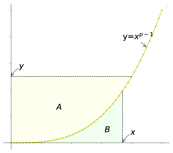
(a) Case 1: $x<y^{1/(p-1)}$ and $p\geq 2$.

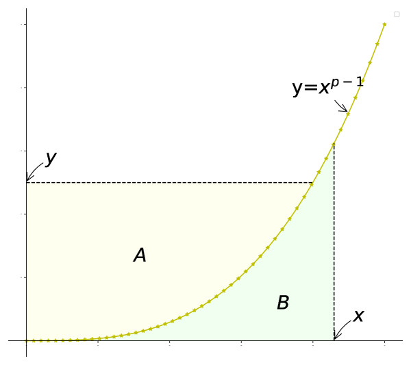
(b) Case 2: $x\geq y^{1/(p-1)}$ and $p\geq 2$.

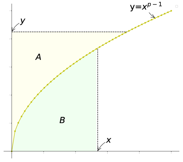
(c) Case 3: $x<y^{1/(p-1)}$ and $1<p<2$.

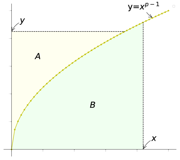
(d) Case 4: $x\geq y^{1/(p-1)}$ and $1<p<2$.

Figure 1.1: Demonstration of Young’s inequality for different cases.

Proof [of Theorem 1.2.2] The area $xy$ is bounded above by the sum of the areas of the two trapezoids with curved edges (the shaded regions $A$ and $B$) as shown in Figure 1.1:

$$\mathrm{area}\,\,\,B=\int_{0}^{x}x^{p-1}dx,\qquad\mathrm{area}\,\,\,A=\int_{0}^{y}y^{1/(p-1)}dy.$$

That is,

$$xy \leq\int_{0}^{x}x^{p-1}dx+\int_{0}^{y}y^{1/(p-1)}dy=\frac{1}{p}x^{p}+\int_{0}^{y}y^{q/p}dy=\frac{1}{p}x^{p}+(\frac{q}{p}+1)^{-1}y^{q/p+1}=\frac{1}{p}x^{p}+\frac{1}{q}y^{q}.$$

This completes the proof.  

There are several conceptually different ways to prove Young’s inequality. As an alternative, we can use the interpolation inequality as follows. For $t\in[0,1]$, we have $$e^{tx+(1-t)y}\leq te^{x}+(1-t)e^{y}.$$

Proof [of Lemma 1.2.2] The function of the scant line through the points $(x,e^{x})$ and $(y,e^{y})$ on the graph of $f(a)=e^{a}$ is (see Figure 1.2):

$$f(t)=(tx+(1-t)y,te^{x}+(1-t)e^{y}).$$

Since the function $f(a)=e^{a}$ is convex, we have

$$e^{tx+(1-t)y}\leq te^{x}+(1-t)e^{y}.$$

This completes the proof.  

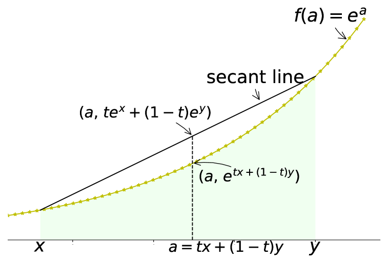
Figure 1.2: Demonstration of interpolation inequality for $e^{x}$.

Using the interpolation inequality for the exponential function, we provide an alternative proof of Theorem 1.2.2.

Proof [of Theorem 1.2.2, an alternative way] We observe that

$$xy =\exp\{\log x+\log y\}=\exp\left\{\frac{q-1}{q}\frac{q}{q-1}\log x+\frac{1}{q}q\log y\right\}.$$

Applying Lemma 1.2.2, we obtain

$$xy \leq\frac{q-1}{q}e^{\frac{q}{q-1}\log x}+\frac{1}{q}e^{q\log y}=\frac{q-1}{q}x^{\frac{q}{q-1}}+\frac{1}{q}y^{q}=\frac{1}{p}x^{p}+\frac{1}{q}y^{q},$$

from which the result follows.  

1.2.3 Hölder’s Inequality

Hölder’s inequality, named after Otto Hölder, is widely used in optimization, machine learning, and many other fields. It is also a generalization of the (vector) Cauchy-Schwarz inequality.

Suppose $p,q>1$ such that $\frac{1}{p}+\frac{1}{q}=1$. Then, for any vector $\bm{x},\bm{y}\in^{n}$, we have $$\sum_{i=1}^{n}x_{i}y_{i}\leq\left\lvert\sum_{i=1}^{n}x_{i}y_{i}\right\rvert\leq\sum_{i=1}^{n}\left\lvert x_{i}\right\rvert\left\lvert y_{i}\right\rvert\leq\left(\sum_{i=1}^{n}\left\lvert x_{i}\right\rvert^{p}\right)^{1/p}\left(\sum_{i=1}^{n}\left\lvert y_{i}\right\rvert^{q}\right)^{1/q}=\left\lVert\bm{x}\right\rVert_{p}\left\lVert\bm{y}\right\rVert_{q},$$ where $\left\lVert\bm{x}\right\rVert_{p}=\left(\sum_{i=1}^{n}\left\lvert x_{i}\right\rvert^{p}\right)^{1/p}$ is known as the $\ell_{p}$ norm or $p$ norm of the vector $\bm{x}$ (see Section 1.3.1). The equality holds if the two sequences $\{\left\lvert x_{i}\right\rvert^{p}\}$ and $\{\left\lvert y_{i}\right\rvert^{q}\}$ are linearly dependent . When $p=q=2$, this reduces to the vector Cauchy-Schwarz inequality (1.2).

Proof [of Theorem 1.2.3] Let $u\triangleq\frac{\left\lvert x_{i}\right\rvert}{\|\bm{x}\|_{p}}$ and $v\triangleq\frac{\left\lvert y_{i}\right\rvert}{\|\bm{y}\|_{q}}$. From Equation (1.4), it follows that

$$uv=\frac{\left\lvert x_{i}\right\rvert\left\lvert y_{i}\right\rvert}{\left\lVert\bm{x}\right\rVert_{p}\left\lVert\bm{y}\right\rVert_{q}}\leq\frac{1}{p}\frac{\left\lvert x_{i}\right\rvert^{p}}{\left\lVert\bm{x}\right\rVert_{p}^{p}}+\frac{1}{q}\frac{\left\lvert y_{i}\right\rvert^{q}}{\left\lVert\bm{y}\right\rVert_{q}^{q}},\qquad\forall\,i\in\{1,2,\ldots,n\}.$$

Therefore,

$$\sum_{i=1}^{n}\frac{\left\lvert x_{i}\right\rvert\left\lvert y_{i}\right\rvert}{\left\lVert\bm{x}\right\rVert_{p}\left\lVert\bm{y}\right\rVert_{q}}\leq\frac{1}{p\left\lVert\bm{x}\right\rVert_{p}^{p}}\sum_{i=1}^{n}\left\lvert x_{i}\right\rvert^{p}+\frac{1}{q\left\lVert\bm{y}\right\rVert_{q}^{q}}\sum_{i=1}^{n}\left\lvert y_{i}\right\rvert^{q}=\frac{1}{p}+\frac{1}{q}=1.$$

That is, $\sum_{i=1}^{n}\left\lvert x_{i}\right\rvert\left\lvert y_{i}\right\rvert\leq\left\lVert\bm{x}\right\rVert_{p}\left\lVert\bm{y}\right\rVert_{q}.$ It is trivial that $\sum_{i=1}^{n}x_{i}y_{i}\leq\sum_{i=1}^{n}\left\lvert x_{i}\right\rvert\left\lvert y_{i}\right\rvert$, from which the result follows.  

Minkowski’s inequality follows immediately from the Hölder’s inequality. Given nonnegative reals $x_{1},x_{2},\ldots,x_{n}\geq 0$ and $y_{1},y_{2},\ldots,y_{n}\geq 0$, and $p\geq 1$, we have $$\left(\sum_{i=1}^{n}(x_{i}+y_{i})^{p}\right)^{1/p}\leq\left(\sum_{i=1}^{n}x_{i}^{p}\right)^{1/p}+\left(\sum_{i=1}^{n}y_{i}^{p}\right)^{1/p}.$$ The equality holds if and only if the sequence $x_{1},x_{2},\ldots,x_{n}$ and $y_{1},y_{2},\ldots,y_{n}$ are proportional. If $p<1$, the inequality sign is reversed. Minkowski’s inequality is essentially the triangle inequality of $\ell_{p}$ norms (Section 1.3.1).

Proof [of Theorem 1.2.3] If $p=1$, the inequality is immediate. We then assume $p>1$. Observe that

$$\sum_{i=1}^{n}(x_{i}+y_{i})^{p}=\sum_{i=1}^{n}x_{i}(x_{i}+y_{i})^{p-1}+\sum_{i=1}^{n}y_{i}(x_{i}+y_{i})^{p-1}.$$

Using Hölder’s inequality, given $p,q$ such that $p>1$ and $\frac{1}{p}+\frac{1}{q}=1$, we have

$$\sum_{i=1}^{n}x_{i}(x_{i}+y_{i})^{p-1} \leq\bigg{(}\sum_{i=1}^{n}x_{i}^{p}\bigg{)}^{1/p}\bigg{(}\sum_{i=1}^{n}(x_{i}+y_{i})^{(p-1)q}\bigg{)}^{1/q}=\bigg{(}\sum_{i=1}^{n}x_{i}^{p}\bigg{)}^{1/p}\bigg{(}\sum_{i=1}^{n}(x_{i}+y_{i})^{p}\bigg{)}^{1/q},$$

$$\sum_{i=1}^{n}y_{i}(x_{i}+y_{i})^{p-1} \leq\bigg{(}\sum_{i=1}^{n}y_{i}^{p}\bigg{)}^{1/p}\bigg{(}\sum_{i=1}^{n}(x_{i}+y_{i})^{(p-1)q}\bigg{)}^{1/q}=\bigg{(}\sum_{i=1}^{n}y_{i}^{p}\bigg{)}^{1/p}\bigg{(}\sum_{i=1}^{n}(x_{i}+y_{i})^{p}\bigg{)}^{1/q}.$$

Combining these results, we obtain

$$\sum_{i=1}^{n}(x_{i}+y_{i})^{p}\leq\bigg{(}\bigg{(}\sum_{i=1}^{n}x_{i}^{p}\bigg{)}^{1/p}+\bigg{(}\sum_{i=1}^{n}y_{i}^{p}\bigg{)}^{1/p}\bigg{)}\bigg{(}\sum_{i=1}^{n}(x_{i}+y_{i})^{p}\bigg{)}^{1/q}.$$

This completes the proof.  

1.3 Norm

The concept of a norm is essential for evaluating the magnitude of vectors and, consequently, allows for the definition of certain metrics on linear spaces equipped with norms. Norms provide a measure of the magnitude of a vector or matrix, which is useful in many applications, such as determining the length of a vector in Euclidean space or the size of a matrix in a multidimensional setting. Additionally, norms enable us to define distances between vectors or matrices. The distance between two vectors $\bm{u}$ and $\bm{v}$ can be computed using the norm of their difference $\left\lVert\bm{u}-\bm{v}\right\rVert$. This is critical for tasks involving proximity measures, such as clustering algorithms in machine learning. 

Definition 1.25 (Vector Norm and Matrix Nrom)

Given a norm $\left\lVert\cdot\right\rVert:^{n}\rightarrow$ on vectors or a norm $\left\lVert\cdot\right\rVert:^{m\times n}\rightarrow$ on matrices, for any vector $\bm{x}\in^{n}$ and any matrix $\bm{A}\in^{m\times n}$, we have   

1. Positive homogeneity. $\left\lVert\lambda\bm{A}\right\rVert=\left\lvert\lambda\right\rvert\cdot\left\lVert\bm{A}\right\rVert$ or $\left\lVert\lambda\bm{x}\right\rVert=\left\lvert\lambda\right\rvert\cdot\left\lVert\bm{x}\right\rVert$ for any $\lambda\in$.

2. Triangle inequality, a.k.a., subadditivity. $\left\lVert\bm{A}+\bm{B}\right\rVert\leq\left\lVert\bm{A}\right\rVert+\left\lVert\bm{B}\right\rVert$, or $\left\lVert\bm{x}+\bm{y}\right\rVert\leq\left\lVert\bm{x}\right\rVert+\left\lVert\bm{y}\right\rVert$ for any matrices $\bm{A},\bm{B}\in^{m\times n}$ or vectors $\bm{x},\bm{y}\in^{n}$.

   1. The triangle inequality also indicates 

      $$\big{|}\,\left\lVert\bm{A}\right\rVert-\left\lVert\bm{B}\right\rVert\,\big{|}\leq\left\lVert\bm{A}-\bm{B}\right\rVert\quad\text{or}\quad\big{|}\,\left\lVert\bm{x}\right\rVert-\left\lVert\bm{y}\right\rVert\,\big{|}\leq\left\lVert\bm{x}-\bm{y}\right\rVert.$$ (1.5)

3. Nonnegativity. $\left\lVert\bm{A}\right\rVert\geq 0$ or $\left\lVert\bm{x}\right\rVert\geq 0$.

   1. the equality holds if and only if $\bm{A}=\mathbf{0}$ or $\bm{x}=\mathbf{0}$.

The vector space ⁿ, together with a given norm $\left\lVert\cdot\right\rVert$, is called a normed vector space. On the other hand, one way to define norms for matrices is by viewing a matrix $\bm{A}\in^{m\times n}$ as a vector in ^mn through its vectorization. What distinguishes a matrix norm is a property called submultiplicativity: $\left\lVert\bm{A}\bm{B}\right\rVert\leq\left\lVert\bm{A}\right\rVert\left\lVert\bm{B}\right\rVert$ if $\left\lVert\cdot\right\rVert$ is a submultiplicative matrix norm (see discussions below). Almost all of the matrix norms we discuss are submultiplicative (Frobenius norm in Proposition 1 and spectral norm in Proposition 1, both of which are special cases of the Schatten $p$-norm, as a consequence of the singular value decomposition (lu2021numerical)).

Definition 1.26 (Orthogonally Invariant Norms)

A matrix norm on ^m×n is orthogonally invariant if $\left\lVert\bm{U}\bm{A}\bm{V}\right\rVert=\left\lVert\bm{A}\right\rVert$ for all orthogonal $\bm{U}\in^{m\times m}$ and $\bm{V}\in^{n\times n}$ and for all $\bm{A}\in^{m\times n}$; and it is weakly orthogonally invariant if $\left\lVert\bm{U}\bm{A}\bm{U}^{\top}\right\rVert=\left\lVert\bm{A}\right\rVert$ for all orthogonal $\bm{U}\in^{m\times m}$ and $\bm{A}\in^{m\times m}$ is square. Similarly, a vector norm on ⁿ is orthogonally invariant if $\left\lVert\bm{Q}\bm{x}\right\rVert=\left\lVert\bm{x}\right\rVert$ for all orthogonal $\bm{Q}\in^{n\times n}$ and for all $\bm{x}\in^{n}$. 

Definition 1.27 (Inner Product)

In most cases, the norm can be derived from the vector inner product $\langle\cdot,\cdot\rangle:^{n}\times^{n}\rightarrow$ (the inner product of vectors $\bm{x},\bm{y}\in^{n}$ is given by $\langle\bm{x},\bm{y}\rangle$), which satisfies the following three axioms: 

1. Commutativity. $\langle\bm{x},\bm{y}\rangle=\langle\bm{y},\bm{x}\rangle$ for any $\bm{x},\bm{y}\in^{n}$.

2. Linearity. $\langle\lambda_{1}\bm{x}_{1}+\lambda_{2}\bm{x}_{2},\bm{y}\rangle=\lambda_{1}\langle\bm{x},\bm{y}\rangle+\lambda_{2}\langle\bm{x}_{2},\bm{y}\rangle$ for any $\lambda_{1},\lambda_{2}\in$ and $\bm{x},\bm{y}\in^{n}$.

3. Nonnegativity. $\langle\bm{x},\bm{x}\rangle\geq 0$ for any $\bm{x}\in^{n}$.

   1. $\langle\bm{x},\bm{x}\rangle=0$ if and only if $\bm{x}=\mathbf{0}$.

Similarly, an inner product for matrices can be defined as a function $\langle\cdot,\cdot\rangle:^{m\times n}\times^{m\times n}\rightarrow$.

For example, the Euclidean inner product, defined as $\left\langle\bm{u},\bm{v}\right\rangle=\bm{u}^{\top}\bm{v},\forall\,\bm{u},\bm{v}\in^{n}$, is an inner product on vectors; the Frobenius inner product, defined as $\left\langle\bm{A},\bm{B}\right\rangle=\mathrm{tr}(\bm{A}^{\top}\bm{B})$, is an inner product on matrices. Unless stated otherwise, we will use the Euclidean inner product throughout this book.

Exercise 1.28 (Cauchy-Schwarz Inequality for Inner Product)

Given an inner product $\langle\cdot,\cdot\rangle:^{n}\times^{n}\rightarrow$, show that

$$\left\lvert\langle\bm{u},\bm{v}\rangle\right\rvert^{2}\leq\left\langle\bm{u},\bm{u}\right\rangle\left\langle\bm{v},\bm{v}\right\rangle\,\,\,\,\,\,\,\,\text{for all }\,\,\,\,\,\,\,\,\bm{u},\bm{v}\in^{n}.$$

Hint: Consider the vector $\bm{x}\triangleq\left\langle\bm{v},\bm{v}\right\rangle\bm{u}-\left\langle\bm{u},\bm{v}\right\rangle\bm{v}$ and analyze $\left\langle\bm{x},\bm{x}\right\rangle\geq 0$.

Exercise 1.29 (Norm Derived from Inner Product, and its Property)

Let $\langle\cdot,\cdot\rangle$ be an inner product on ${}^{n}\times^{n}$. Then the function $\left\lVert\cdot\right\rVert=\langle\cdot,\cdot\rangle^{1/2}:^{n}\rightarrow[0,\infty)$ is a norm on ⁿ. Show that the function satisfies

$$\textbf{(Parallelogram identity):}\,\,\left\lVert\bm{u}+\bm{v}\right\rVert^{2}+\left\lVert\bm{u}-\bm{v}\right\rVert^{2}=2(\left\lVert\bm{u}\right\rVert^{2}+\left\lVert\bm{v}\right\rVert^{2}),\,\,\forall\,\bm{u},\bm{v}\in^{n}.$$ (1.6)

(This is known as the parallelogram identity: consider a parallelogram in a vector space where the sides are represented by the vectors $\bm{u}$ and $\bm{v}$, the diagonals of this parallelogram are represented by the vectors $\bm{u}+\bm{v}$ and $\bm{u}-\bm{v}$.) Prove the following polarization identity:

$$\textbf{(Polarization identity):}\,\,\,\,\,\,\,\,\left\langle\bm{u},\bm{v}\right\rangle=\frac{1}{4}(\left\lVert\bm{u}+\bm{v}\right\rVert^{2}-\left\lVert\bm{u}-\bm{v}\right\rVert^{2}).$$ (1.7)

Therefore, the vector space ⁿ, when equipped with an inner product $\left\langle\cdot,\cdot\right\rangle$, is called an inner product space, which is also a normed vector space with the derived norm.

1.3.1 Vector Norm

The vector norm is derived from the definition of the inner product. In most cases, the inner product in ⁿ is implicitly referred to as the dot product (a.k.a., Euclidean inner product), defined by $\langle\bm{x},\bm{y}\rangle=\sum_{i=1}^{n}x_{i}y_{i}.$ The $\ell_{2}$ norm (also called the $\ell_{2}$ vector norm) is induced by the dot product and is given by $\left\lVert\bm{x}\right\rVert_{2}=\sqrt{\langle\bm{x},\bm{x}\rangle}=\sqrt{\sum_{i=1}^{n}x_{i}^{2}}.$ More generally, for any $p\geq 1$ , the $\ell_{p}$ norm (a.k.a., the $\ell_{p}$ vector norm or Hölder’s norm) is given by

$$\textbf{($\ell_{p}$ {norm})}:\qquad\left\lVert\bm{x}\right\rVert_{p}=\sqrt[p]{\sum_{i=1}^{n}\left\lvert x_{i}\right\rvert^{p}},\quad p\geq 1.$$ (1.8)

This norm satisfies positive homogeneity and nonnegativity by definition, while the triangle inequality follows from Minkowski’s inequality (Theorem 1.2.3; alternatively, we can prove the triangle inequality for the $\ell_{p}$ norm using Hölder’s inequality; see Exercise 1.30). From the general definition of the $\ell_{p}$ norm, the $\ell_{1}$ and $\ell_{\infty}$ norms can be obtained by, respectively,

$$\left\lVert\bm{x}\right\rVert_{1}=\sum_{i=1}^{n}\left\lvert x_{i}\right\rvert\,\,\,\,\,\,\,\,\text{and}\,\,\,\,\,\,\,\,\left\lVert\bm{x}\right\rVert_{\infty}=\mathop{\max}_{i=1,2,\ldots,n}\left\lvert x_{i}\right\rvert.$$

Following the definition of the $\ell_{p}$ norm, we can obtain the famous Hölder’s inequality in Theorem 1.2.3. Thus, the $\ell_{p}$ norm is sometimes referred to as Hölder’s norm. Conversely, Hölder’s inequality can be used to prove the validity of the $\ell_{p}$ norm. This proof is left as an exercise; see, for example, lu2021numerical.

Exercise 1.30 (Triangle Inequality)

Prove the triangle inequality for the $\ell_{p}$ norm using Hölder’s inequality. For the special case $p=2$, use the Cauchy-Schwartz inequlaity (Proposition 1.2.1) to prove the triangle inequality.

Exercise 1.31 (Orthogonal Invariance of $\ell_{2}$)

Show that the $\ell_{2}$ norm is orthogonally invariant: $\left\lVert\bm{Q}\bm{x}\right\rVert_{2}=\left\lVert\bm{x}\right\rVert_{2}$ for all $\bm{x}\in^{n}$ if $\bm{Q}$ is orthogonal. Investigate whether this property holds for other $\ell_{p}$ norms.

Properties

For any vector norm, we also have the following properties. Given any $\bm{x}\in^{n}$, the function $f(p)=\left\lVert\bm{x}\right\rVert_{p}$ is nonincreasing for $p=[1,\infty)$. Therefore, $$\left\lVert\bm{x}\right\rVert_{\infty}\leq\left\lVert\bm{x}\right\rVert_{q}\leq\left\lVert\bm{x}\right\rVert_{p}\leq\left\lVert\bm{x}\right\rVert_{2}\leq\left\lVert\bm{x}\right\rVert_{1},\quad\text{if }\infty\geq q\geq p\geq 2\geq 1.$$ (1.9) If $\bm{x}$ has at least two nonzero elements, the inequalities can be strict. This behavior can also be observed in the figures of unit balls (Figure 1.3). Moreover, for any $\infty\geq p\geq 1$, we also have the bound $$\left\lVert\bm{x}\right\rVert_{\infty}\leq\left\lVert\bm{x}\right\rVert_{p}\leq n^{1/p}\left\lVert\bm{x}\right\rVert_{\infty},\quad\text{if }\infty\geq p\geq 1.$$ (1.10)

Proof [of Proposition 1] Let $S(p)\triangleq\left\lVert\bm{x}\right\rVert_{p}^{p}$. Taking the logarithm of $f(p)$ gives $\ln f(p)=\frac{1}{p}\ln S(p).$ Differentiate both sides with respect to $p$:

$$\frac{f^{\prime}(p)}{f(p)}=\frac{d}{dp}\left(\frac{1}{p}\ln S(p)\right)=-\frac{1}{p^{2}}\ln S(p)+\frac{1}{p}\cdot\frac{S^{\prime}(p)}{S(p)}.$$

This shows

$$f^{\prime}(p)=f(p)\left(-\frac{1}{p^{2}}\ln S(p)+\frac{1}{p}\cdot\frac{S^{\prime}(p)}{S(p)}\right)=\frac{1}{p}\left\lVert\bm{x}\right\rVert_{p}^{1-p}\sum_{i=1}^{n}\alpha_{i},$$

where

$$S^{\prime}(p)=\sum_{i=1}^{n}\left\lvert x_{i}\right\rvert^{p}\ln\left\lvert x_{i}\right\rvert\quad\text{and}\quad\alpha_{i}=\left\{\begin{aligned} &\left\lvert x_{i}\right\rvert^{p}(\ln\left\lvert x_{i}\right\rvert-\ln\left\lVert\bm{x}\right\rVert_{p}),&\text{if }x_{i}\neq 0;\\ &0,&\text{if }x_{i}=0.\end{aligned}\right.$$

This shows $f^{\prime}(p)\leq 0$ since $\ln\left\lvert x_{i}\right\rvert-\ln\left\lVert\bm{x}\right\rVert_{p}\leq 0$. If $\bm{x}$ has at least two nonzero elements, $f^{\prime}(p)<0$ and $f(p)$ is decreasing.

For the second part, following the definition of the $\ell_{p}$ norm, we notice that

$$(\left\lVert\bm{x}\right\rVert_{\infty})^{p}=\left(\mathop{\max}_{i=1,2,\ldots,n}\left\lvert x_{i}\right\rvert\right)^{p}\leq\sum_{i=1}^{n}\left\lvert x_{i}\right\rvert^{p}\leq n\mathop{\max}_{i=1,2,\ldots,n}\left\lvert x_{i}\right\rvert^{p}=n(\left\lVert\bm{x}\right\rVert_{\infty})^{p},$$

from which the result follows.  

Let $\left\lVert\cdot\right\rVert$ be an orthogonally invariant norm on ⁿ, and let $\left\lVert\cdot\right\rVert_{2}$ be the $\ell_{2}$ norm. Then, for any $\bm{x}\in^{n}$, we have $\left\lVert\bm{x}\right\rVert=\left\lVert\bm{x}\right\rVert_{2}\left\lVert\bm{e}_{1}\right\rVert$.

Proof [of Proposition 1] Define $\gamma\triangleq\left\lVert\bm{x}\right\rVert_{2}$ and let $\widehat{\bm{x}}\triangleq\bm{x}/\gamma$, so that $\bm{x}=\gamma\widehat{\bm{x}}$. Consider an orthogonal matrix $\bm{U}$ whose first column is $\widehat{\bm{x}}$. By the definition of a norm and the orthogonally invariant property, we have $\left\lVert\bm{x}\right\rVert=\gamma\left\lVert\widehat{\bm{x}}\right\rVert=\gamma\left\lVert\bm{U}\bm{e}_{1}\right\rVert=\gamma\left\lVert\bm{e}_{1}\right\rVert$.  
The result also implies that the $\ell_{2}$ norm is the only orthogonally invariant norm satisfying $\left\lVert\bm{e}_{1}\right\rVert=1$.

We conclude this section by introducing an important property of vector norms that is frequently useful. The following theorem on the equivalence of vector norms states that if a vector is small in one norm, it is also small in another norm, and vice versa. Let $\left\lVert\cdot\right\rVert_{a}$ and $\left\lVert\cdot\right\rVert_{b}$ be two different vector norms, where $\left\lVert\cdot\right\rVert_{a}$, $\left\lVert\cdot\right\rVert_{b}$: ${}^{n}\rightarrow$. Then, there exist positive scalars $\alpha$ and $\beta$ such that for all $\bm{x}\in^{n}$, the following inequality holds: $$\alpha\left\lVert\bm{x}\right\rVert_{a}\leq\left\lVert\bm{x}\right\rVert_{b}\leq\beta\left\lVert\bm{x}\right\rVert_{a}.$$ This implies $$\frac{1}{\beta}\left\lVert\bm{x}\right\rVert_{b}\leq\left\lVert\bm{x}\right\rVert_{a}\leq\frac{1}{\alpha}\left\lVert\bm{x}\right\rVert_{b}.$$ This justifies the term “equivalence” in the theorem.

Proof [of Theorem 1] In advanced calculus, it is stated that $\mathop{\sup}_{\bm{x}\in{\mathbb{S}}}f(\bm{x})$ is attained for some vector $\bm{x}\in{\mathbb{S}}$ as long as $f(\cdot)$ is continuous and ${\mathbb{S}}$ is a compact set (closed and bounded); see Theorem LABEL:theorem:weierstrass_them. When the supremum is an element in the set ${\mathbb{S}}$, this supremum is known as the maximum such that $\mathop{\sup}_{\bm{x}\in{\mathbb{S}}}f(\bm{x})=\mathop{\max}_{\bm{x}\in{\mathbb{S}}}f(\bm{x})$. Without loss of generality, we assume $\bm{x}\neq\mathbf{0}$. Then we have:

$$\left\lVert\bm{x}\right\rVert_{b} =\frac{\left\lVert\bm{x}\right\rVert_{b}}{\left\lVert\bm{x}\right\rVert_{a}}\left\lVert\bm{x}\right\rVert_{a}\leq\mathop{\sup}_{\bm{z}\neq 0}\frac{\left\lVert\bm{z}\right\rVert_{b}}{\left\lVert\bm{z}\right\rVert_{a}}\left\lVert\bm{x}\right\rVert_{a}=\mathop{\sup}_{\left\lVert\bm{y}\right\rVert_{a}=1}\left\lVert\bm{y}\right\rVert_{b}\left\lVert\bm{x}\right\rVert_{a}=\left\lVert\bm{x}\right\rVert_{a}\mathop{\max}_{\left\lVert\bm{y}\right\rVert_{a}=1}\left\lVert\bm{y}\right\rVert_{b}.$$

The last equality holds since $\{\bm{y}:\left\lVert\bm{y}\right\rVert_{a}=1\}$ is a compact set. By setting $\beta\triangleq\mathop{\max}_{\left\lVert\bm{y}\right\rVert_{a}=1}\left\lVert\bm{y}\right\rVert_{b}$, we have $\left\lVert\bm{x}\right\rVert_{b}\leq\beta\left\lVert\bm{x}\right\rVert_{a}$. From the above argument, there exists a $\tau$ such that $\left\lVert\bm{x}\right\rVert_{a}\leq\tau\left\lVert\bm{x}\right\rVert_{b}.$ Letting $\alpha\triangleq\frac{1}{\tau}$, we obtain $\alpha\left\lVert\bm{x}\right\rVert_{a}\leq\left\lVert\bm{x}\right\rVert_{b}$, from which the result follows.  

Example 1.35 (Equivalence of Vector Norms)

The following inequalities hold for all $\bm{x}\in^{n}$:

$$\left\lVert\bm{x}\right\rVert_{\infty} \leq\left\lVert\bm{x}\right\rVert_{1}\leq n\left\lVert\bm{x}\right\rVert_{\infty};$$

$$\left\lVert\bm{x}\right\rVert_{\infty} \leq\left\lVert\bm{x}\right\rVert_{2}\leq\sqrt{n}\left\lVert\bm{x}\right\rVert_{\infty};$$

$$\left\lVert\bm{x}\right\rVert_{2} \leq\left\lVert\bm{x}\right\rVert_{1}\leq\sqrt{n}\left\lVert\bm{x}\right\rVert_{2}.$$

This demonstrates the equivalence of the $\ell_{1},\ell_{2}$, and $\ell_{\infty}$ vector norms. $\square$

Dual Norm

Consider the $\ell_{p}$ vector norm. From Hölder’s inequality (Theorem 1.2.3), we have $\bm{x}^{\top}\bm{y}\leq\left\lVert\bm{x}\right\rVert_{p}\left\lVert\bm{y}\right\rVert_{q},$ where $p,q>1$ satisfy $\frac{1}{p}+\frac{1}{q}=1$, and $\bm{x},\bm{y}\in^{n}$. Equality holds if the two sequences $\{\left\lvert x_{i}\right\rvert^{p}\}$ and $\{\left\lvert y_{i}\right\rvert^{q}\}$ are linearly dependent. This implies

$$\mathop{\max}_{\left\lVert\bm{y}\right\rVert_{q}=1}\bm{x}^{\top}\bm{y}=\left\lVert\bm{x}\right\rVert_{p}.$$ (1.11)

For this reason, $\left\lVert\cdot\right\rVert_{q}$ is called the dual norm of $\left\lVert\cdot\right\rVert_{p}$. On the other hand, for each $\bm{x}\in^{n}$ with $\left\lVert\bm{x}\right\rVert_{p}=1$, there exists a vector $\bm{y}\in^{n}$ such that $\left\lVert\bm{y}\right\rVert_{q}=1$ and $\bm{x}^{\top}\bm{y}=1$. Notably, the $\ell_{2}$ norm is self-dual, while the $\ell_{1}$ and $\ell_{\infty}$ norms are dual to each other.

Definition 1.36 (Set of Primal Counterparts)

Let $\left\lVert\cdot\right\rVert$ be any norm on ⁿ. Then the set of primal counterparts of $\bm{a}$ is defined as

$$\Lambda_{\bm{a}}=\operatorname*{\text{arg max}}_{\bm{u}\in^{n}}\left\{\left\langle\bm{a},\bm{u}\right\rangle\mid\left\lVert\bm{u}\right\rVert\leq 1\right\}.$$ (1.12)

That is, $\left\langle\bm{a},\bm{a}^{\dagger}\right\rangle=\left\lVert\bm{a}\right\rVert_{*}$ for any $\bm{a}^{\dagger}\in\Lambda_{\bm{a}}$, where $\left\lVert\cdot\right\rVert_{*}$ denotes the dual norm. It follows that

1. If $\bm{a}\neq\mathbf{0}$, then $\left\lVert\bm{a}^{\dagger}\right\rVert=1$ for any $\bm{a}^{\dagger}\in\Lambda_{\bm{a}}$.

2. If $\bm{a}=\mathbf{0}$, then $\Lambda_{\bm{a}}=\{\bm{x}\in^{n}\mid\left\lVert\bm{x}\right\rVert\leq 1\}$.

Example 1.37 (Set of Primal Counterparts)

A few examples for the sets of primal counterparts are shown below:

• If the norm is the $\ell_{2}$ norm, then for any $\bm{a}\neq\mathbf{0}$, $\Lambda_{\bm{a}}=\left\{{\bm{a}}/{\left\lVert\bm{a}\right\rVert_{2}}\right\}.$

• If the norm is the $\ell_{1}$ norm, then for any $\bm{a}\neq\mathbf{0}$,

  $$\Lambda_{\bm{a}}=\left\{\sum_{i\in{\mathbb{I}}(\bm{a})}\lambda_{i}\operatorname{sign}(a_{i})\bm{e}_{i}\mid\sum_{i\in{\mathbb{I}}(\bm{a})}\lambda_{i}=1,\lambda_{j}\geq 0,j\in{\mathbb{I}}(\bm{a})\right\},$$

  where ${\mathbb{I}}(\bm{a})\triangleq\operatorname*{\text{arg max}}_{i=1,2,\ldots,n}|a_{i}|$.

• If the norm is the $\ell_{\infty}$ norm, then for any $\bm{a}\neq\mathbf{0}$,

  $$\Lambda_{\bm{a}}=\left\{\bm{x}\in^{n}\mid x_{i}=\operatorname{sign}(a_{i}),i\in{\mathbb{I}}_{\neq}(\bm{a}),|x_{j}|\leq 1,j\in{\mathbb{I}}_{0}(\bm{a})\right\},$$

  where ${\mathbb{I}}_{\neq}(\bm{a})\triangleq\left\{i\in\{1,2,\ldots,n\}\mid a_{i}\neq 0\right\}$ and ${\mathbb{I}}_{0}(\bm{a})\triangleq\left\{i\in\{1,2,\ldots,n\}\mid a_{i}=0\right\}.$

These examples play a crucial role in the development of non-Euclidean gradient descent methods, which will be discussed in Sections LABEL:section:als-gradie-descent-taylor and LABEL:section:noneucli_gd. $\square$

Unit Ball

The unit ball of a norm is the set of all points whose distance from the origin (i.e., the zero vector) equals 1. If the distance is defined by the $\ell_{p}$ norm, the unit ball is the collection of

$${\mathbb{B}}_{p}=\{\bm{x}:\left\lVert\bm{x}\right\rVert_{p}=1\}.$$

The comparison of the $\ell_{p}$ norm in three-dimensional space with different values of $p$ is depicted in Figure 1.3.

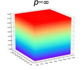
(a) $p=\infty$.

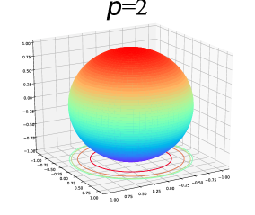
(b) $p=2$.

(c) $p=1$.

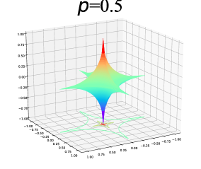
(d) $p=0.5$.

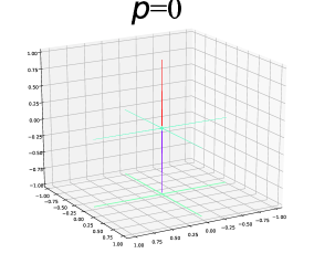
(e) $p=0$.

Figure 1.3: Unit ball of $\ell_{p}$ norms in three-dimensional space. When $p<1$, the metric does not qualify as a norm since it does not satisfy the third axiom of the norm in Definition 1.25.

Vector norms are fundamental in machine learning. In Section LABEL:section:pre_ls, we will discuss how least squares aim to minimize the squared distance between the observed value $\bm{b}$ and the predicted value $\bm{A}\bm{x}$: $\left\lVert\bm{A}\bm{x}-\bm{b}\right\rVert_{2}$, which is the $\ell_{2}$ norm of $\bm{A}\bm{x}-\bm{b}$. Alternatively, minimizing the $\ell_{1}$ norm of the difference between the observed and predicted values can yield a more robust estimation of $\bm{x}$, particularly in the presence of outliers (zoubir2012robust).

$\bm{Q}$-Inner Product, $\bm{Q}$-Norm, $\bm{S}$-Norm

The standard dot product is not the only possible inner product that can be defined on ⁿ. Given a positive definite $n\times n$ matrix $\bm{Q}$, a $\bm{Q}$-dot product can be defined as 

$$\langle\bm{x},\bm{y}\rangle_{\bm{Q}}=\bm{x}^{\top}\bm{Q}\bm{y}.$$

One can verify that the $\bm{Q}$-dot product defined above satisfies the three axioms of an inner product, as discussed at the beginning of this section. When $\bm{Q}=\bm{I}$, this reduces to the standard Euclidean inner product (dot product). From the $\bm{Q}$-dot product, we can define the corresponding $\bm{Q}$-$\ell_{2}$-norm as $\left\lVert\bm{x}\right\rVert_{\bm{Q},2}=\sqrt{\bm{x}^{\top}\bm{Q}\bm{x}}.$ More generally, given a positive definite matrix $\bm{Q}\in^{n\times n}$ and a general norm $\left\lVert\cdot\right\rVert$ on ⁿ, we define the $\bm{Q}$-norm as:

$$\textbf{$\bm{Q}$-norm:}\qquad\left\lVert\bm{x}\right\rVert_{\bm{Q}}=\left\lVert\sqrt{\bm{Q}}\bm{x}\right\rVert$$ (1.13)

Similarly, given a matrix $\bm{S}\in^{m\times n}$ with full column rank and a general norm $\left\lVert\cdot\right\rVert$ on ^m, the $\bm{S}$-norm is defined as:

$$\textbf{$\bm{S}$-norm:}\qquad\left\lVert\bm{x}\right\rVert_{\bm{S}}=\left\lVert\bm{S}\bm{x}\right\rVert,$$ (1.14)

which is a norm on ⁿ. To establish this rigorously, we introduce the following lemma. Let $\left\lVert\cdot\right\rVert$ be a norm on ^m. Given a matrix $\bm{S}\in^{m\times n}$, then $\left\lVert\bm{S}(\cdot)\right\rVert$ defines a semi-norm  on ⁿ. If $\bm{S}$ has full column rank $n$, then $\left\lVert\bm{S}(\cdot)\right\rVert$ is a norm on ^m.

Proof [of Lemma 1] For any vectors $\bm{x},\bm{y}\in^{m}$, following from Definition 1.25, we have

$$\left\lVert\bm{x}\right\rVert\geq 0,\,\,\,\,\,\,\,\,\left\lVert\lambda\bm{x}\right\rVert=\left\lvert\lambda\right\rvert\cdot\left\lVert\bm{x}\right\rVert,\,\,\,\,\,\,\,\,\left\lVert\bm{x}+\bm{y}\right\rVert\leq\left\lVert\bm{x}\right\rVert+\left\lVert\bm{y}\right\rVert.$$

Now, for any $\bm{c},\bm{d}\in^{n}$, it follows that:

$$\left\lVert\bm{S}\bm{c}\right\rVert\geq 0,\,\,\,\,\,\,\,\,\left\lVert\lambda\bm{S}\bm{c}\right\rVert=\left\lvert\lambda\right\rvert\cdot\left\lVert\bm{S}\bm{c}\right\rVert,\,\,\,\,\,\,\,\,\left\lVert\bm{S}\bm{c}+\bm{S}\bm{d}\right\rVert\leq\left\lVert\bm{S}\bm{c}\right\rVert+\left\lVert\bm{S}\bm{b}\right\rVert.$$

Therefore, $\left\lVert\bm{S}(\cdot)\right\rVert$ is a semi-norm. If $\bm{S}$ has full column rank, $\bm{S}\bm{c}=\mathbf{0}$ only if $\bm{c}=\mathbf{0}$, ensuring that $\left\lVert\bm{S}(\cdot)\right\rVert$ satisfies the norm definiteness property. Hence, it is a norm. This completes the proof.  

Exercise 1.39 (Weighted $\ell_{p}$ Norm)

Let $w_{1},w_{2},\ldots,w_{p}$ be positive real numbers, and let $p\geq 1$. Show that the weighted $\ell_{p}$ norm $\left\lVert\bm{x}\right\rVert=\sqrt[p]{\sum_{i=1}^{n}w_{i}\left\lvert x_{i}\right\rvert^{p}}$ is a valid norm on ⁿ. Hint: Show that it is a norm of the form $\left\lVert\bm{S}\bm{x}\right\rVert_{p}$.

1.3.2 Matrix Norm

Submultiplicativity of Matrix Norms

In some texts, a matrix norm that is not submultiplicative is referred to as a vector norm on matrices or a generalized matrix norm. The submultiplicativity of a matrix norm plays a crucial role in the analysis of square matrices. However, it’s important to note that the definition of a matrix norm applies to both square and rectangular matrices. For a submultiplicative matrix norm $\left\lVert\cdot\right\rVert$ satisfying $\left\lVert\bm{A}\bm{B}\right\rVert\leq\left\lVert\bm{A}\right\rVert\left\lVert\bm{B}\right\rVert$, considering $\bm{A}\in^{n\times n}$, it follows that

$$\left\lVert\bm{A}^{2}\right\rVert\leq\left\lVert\bm{A}\right\rVert^{2}\quad\implies\quad\left\lVert\bm{A}^{k}\right\rVert\leq\left\lVert\bm{A}\right\rVert^{k},\forall\,k\in\{1,2,\ldots,\}.$$ (1.15)

Therefore, if the matrix is idempotent, i.e., $\bm{A}^{2}=\bm{A}$, we have $\left\lVert\bm{A}\right\rVert\geq 1$. This also indicates:

$$\left\lVert\bm{I}\right\rVert\geq 1,\quad\text{if}\quad\left\lVert\cdot\right\rVert\text{ is submultiplicative}.$$ (1.16)

On the other hand, if $\bm{A}$ is nonsingular, then for submultiplicative norms, we have the inequality:

$$1\leq\left\lVert\bm{I}\right\rVert=\left\lVert\bm{A}\bm{A}^{-1}\right\rVert\leq\left\lVert\bm{A}\right\rVert\left\lVert\bm{A}^{-1}\right\rVert.$$

This means that for a submultiplicative norm, $\left\lVert\bm{I}\right\rVert\geq 1$, and it is considered normalized if and only if $\left\lVert\bm{I}\right\rVert=1$.

Bounds on the spectral radius.

The property of submultiplicativity can be utilized to establish bounds on the spectral radius of a matrix (i.e., the largest magnitude of the eigenvalues of a matrix). Given an eigenpair $(\lambda,\bm{x})$ of a matrix $\bm{A}\in^{n\times n}$, and consider the matrix $\bm{X}=\bm{x}\mathbf{1}^{\top}=[\bm{x},\bm{x},\ldots,\bm{x}]$. For a submultiplicative matrix norm $\left\lVert\cdot\right\rVert$ on ^n×n, it holds that $\left\lvert\lambda\right\rvert\left\lVert\bm{X}\right\rVert=\left\lVert\lambda\bm{X}\right\rVert=\left\lVert\bm{A}\bm{X}\right\rVert\leq\left\lVert\bm{A}\right\rVert\left\lVert\bm{X}\right\rVert.$ Thus, the spectral radius is bounded by the matrix norm $\left\lVert\bm{A}\right\rVert$. Similarly, we can prove that $\left\lvert\lambda^{-1}\right\rvert\leq\left\lVert\bm{A}^{-1}\right\rVert$. Consequently, we obtain lower and upper bounds on the spectral radius $\rho(\bm{A})$:

$$\textbf{Bounds on spectral radius:}\qquad\frac{1}{\left\lVert\bm{A}^{-1}\right\rVert}\leq\rho(\bm{A})\leq\left\lVert\bm{A}\right\rVert.$$ (1.17)

Additionally, the submultiplicative property aids in understanding bounds on the spectral radius of the product of matrices. For instance, given matrices $\bm{A}$ and $\bm{B}$ (provided the matrix product $\bm{A}\bm{B}$ is defined), we have

$$\rho(\bm{A}\bm{B})\leq\left\lVert\bm{A}\bm{B}\right\rVert\leq\left\lVert\bm{A}\right\rVert\left\lVert\bm{B}\right\rVert.$$ (1.18)

Power of square matrices.

When $\left\lVert\bm{A}\right\rVert\leq 1$ for a square matrix $\bm{A}\in^{n\times n}$, (1.15) shows that $\left\lVert\bm{A}^{k}\right\rVert\leq\left\lVert\bm{A}\right\rVert^{k}\stackrel{{\scriptstyle k\rightarrow\infty}}{{=}}0$. This holds true regardless of the specific norm used, provided it is submultiplicative. Thus, if $\bm{A}^{k}$ tends to the zero matrix when $k\rightarrow\infty$ if $\left\lVert\bm{A}\right\rVert\leq 1$. A matrix with this property is called convergent. The convergence of a matrix can also be characterized by its spectral radius.

Exercise 1.40 (Convergence Matrices)

Let $\bm{A}\in^{n\times n}$. Show that $\mathop{\lim}_{k\rightarrow\infty}\bm{A}^{k}=\mathbf{0}$ if and only if the spectral radius $\rho(\bm{A})<1$. Hint: Examine $\bm{A}^{k}\bm{x}=\lambda^{k}\bm{x}$.

Exercise 1.41 (Convergence Matrices)

Let $\bm{A}\in^{n\times n}$ and $\epsilon>0$. Show that there is a constant $C=C(\bm{A},\epsilon)$ such that $\left\lvert(\bm{A}^{k})_{ij}\right\rvert\leq C(\rho(\bm{A})+\epsilon)^{k}$ for $k\in\{1,2,\ldots\},i,j\in\{1,2,\ldots,n\}$. Hint: Use Exercise 1.40 and examine $\bm{B}=\frac{1}{\rho(\bm{A})+\epsilon}\bm{A}$, whose spectral radius is strictly less than 1.

The Gelfand formula offers a method to estimate the spectral radius of a matrix using submultiplicative norms.

Exercise 1.42 (Gelfand Formula)

Let $\bm{A}\in^{n\times n}$ and let $\left\lVert\cdot\right\rVert$ be a submultiplicative matrix norm on ^n×n. Show that $\rho(\bm{A})=\mathop{\lim}_{k\rightarrow\infty}\left\lVert\bm{A}^{k}\right\rVert^{1/k}$. Hint: Consider $\rho(\bm{A}^{k})=\rho(\bm{A})^{k}\leq\left\lVert\bm{A}\right\rVert$ and examine $\bm{B}=\frac{1}{\rho(\bm{A})+\epsilon}\bm{A}$, whose spectral radius is strictly less than 1.

Frobenius Norm

The norm of a matrix serves a similar purpose to the norm of a vector. One important matrix norm is the Frobenius norm, which can be considered the matrix equivalent of the $\ell_{2}$ vector norm.

Definition 1.43 (Frobenius Norm)

The Frobenius norm of a matrix $\bm{A}\in^{m\times n}$ is defined as

$$\left\lVert\bm{A}\right\rVert_{F}=\sqrt{\sum_{i=1,j=1}^{m,n}(a_{ij})^{2}}=\sqrt{\mathrm{tr}(\bm{A}\bm{A}^{\top})}=\sqrt{\mathrm{tr}(\bm{A}^{\top}\bm{A})}=\sqrt{\sigma_{1}^{2}+\sigma_{2}^{2}+\ldots+\sigma_{r}^{2}},$$

where the values of $\sigma_{i}$ are the singular values of $\bm{A}$, and $r$ is the rank of $\bm{A}$. This represents the square root of the sum of the squares of all elements in $\bm{A}$.

The equivalence of $\sqrt{\sum_{i=1,j=1}^{m,n}(a_{ij})^{2}}$, $\sqrt{\mathrm{tr}(\bm{A}\bm{A}^{\top})}$, and $\sqrt{\mathrm{tr}(\bm{A}^{\top}\bm{A})}$ is straightforward. The equivalence between $\sqrt{\mathrm{tr}(\bm{A}\bm{A}^{\top})}$ and $\sqrt{\sigma_{1}^{2}+\sigma_{2}^{2}+\ldots+\sigma_{r}^{2}}$ can be shown using the singular value decomposition (SVD). Suppose $\bm{A}$ admits the SVD $\bm{A}=\bm{U}\boldsymbol{\Sigma}\bm{V}^{\top}$, then:

$$\sqrt{\mathrm{tr}(\bm{A}\bm{A}^{\top})}=\sqrt{\mathrm{tr}(\bm{U}\boldsymbol{\Sigma}\bm{V}^{\top}\bm{V}\boldsymbol{\Sigma}\bm{U}^{\top})}=\sqrt{\mathrm{tr}(\boldsymbol{\Sigma}^{2})}=\sqrt{\sigma_{1}^{2}+\sigma_{2}^{2}+\ldots+\sigma_{r}^{2}}.$$

Apparently, the Frobenius norm can also be defined using the vector $\ell_{2}$ norm such that $\left\lVert\bm{A}\right\rVert_{F}=\sqrt{\sum_{i=1}^{n}\left\lVert\bm{a}_{i}\right\rVert^{2}}$, where $\bm{a}_{i}$ for all $i\in\{1,2,\ldots,n\}$ are the columns of $\bm{A}$.

The Frobnenius norm is submultiplicative. That is, $\left\lVert\bm{A}\bm{B}\right\rVert_{F}\leq\left\lVert\bm{A}\right\rVert_{F}\left\lVert\bm{B}\right\rVert_{F}$.

Proof [of Proposition 1] Suppose $\bm{A}\in^{m\times n}$ and $\bm{B}\in^{n\times p}$. We have

$$\left\lVert\bm{A}\bm{B}\right\rVert_{F}=\bigg{(}\sum_{i,j=1}^{m,p}\big{(}\sum_{k=1}^{n}a_{ik}b_{kj}\big{)}^{2}\bigg{)}^{1/2}\leq\bigg{(}\sum_{i,j=1}^{m,p}\big{(}\sum_{k=1}^{n}a_{ik}^{2}\big{)}\big{(}\sum_{k=1}^{n}b_{kj}^{2}\big{)}\bigg{)}^{1/2}=\left\lVert\bm{A}\right\rVert_{F}\left\lVert\bm{B}\right\rVert_{F}.$$

This completes the proof.  

Let $\bm{A}\in^{m\times n}$ be given, and let $\bm{U}\in^{m\times m}$ and $\bm{V}\in^{n\times n}$ be orthogonal matrices. Then, $\left\lVert\bm{A}\right\rVert_{F}=\left\lVert\bm{U}\bm{A}\bm{V}\right\rVert_{F}.$

Proof [of Proposition 1] We observe that

$$\left\lVert\bm{U}\bm{A}\bm{V}\right\rVert_{F} =\sqrt{\mathrm{tr}((\bm{U}\bm{A}\bm{V})(\bm{U}\bm{A}\bm{V})^{\top})}=\sqrt{\mathrm{tr}(\bm{U}\bm{A}\bm{A}^{\top}\bm{U}^{\top})}$$

$$=\sqrt{\mathrm{tr}(\bm{A}\bm{A}^{\top}\bm{U}^{\top}\bm{U})}=\sqrt{\mathrm{tr}(\bm{A}\bm{A}^{\top})}=\left\lVert\bm{A}\right\rVert_{F},$$

where the third equality holds due to the cyclic property of the trace.  

The Frobenius norm is defined as the square root of the sum of the squares of the matrix elements. Additionally, we have the well-known Schur inequality, which follows from the definition of the Frobenius norm. Let $\lambda_{1},\lambda_{2},\ldots,\lambda_{n}$ be real eigenvalues of the matrix $\bm{A}\in^{n\times n}$. Then, $\sum_{i=1}^{n}\left\lvert\lambda_{i}\right\rvert^{2}\leq\sum_{i=1,j=1}^{n,n}\left\lvert a_{ij}\right\rvert^{2}=\left\lVert\bm{A}\right\rVert_{F}^{2},$ which means the sum of the squared absolute values of the eigenvalues is bounded by the Frobenius norm of the matrix.

Proof [of Theorem 1] Suppose the Schur decomposition of $\bm{A}$ is given by $\bm{A}=\bm{Q}\bm{U}\bm{Q}^{\top}$ (see, for example, lu2021numerical), where the diagonal of $\bm{U}$ contains the eigenvalues of $\bm{A}$. By the orthogonal invariance Proposition 1, we have $\left\lVert\bm{U}\right\rVert_{F}=\left\lVert\bm{Q}\bm{U}\bm{Q}^{\top}\right\rVert_{F}=\left\lVert\bm{A}\right\rVert_{F}.$ Therefore,

$$\sum_{i=1}^{n}\left\lvert\lambda_{i}\right\rvert^{2}=\sum_{i=1}^{n}u_{ii}^{2}\leq\sum_{i=1}^{n}u_{ii}^{2}+\sum_{i\neq j}u_{ij}^{2}=\left\lVert\bm{U}\right\rVert_{F}^{2}\quad\implies\quad\sum_{i=1}^{n}\left\lvert\lambda_{i}\right\rvert^{2}\leq\left\lVert\bm{A}\right\rVert_{F}^{2}.$$

This completes the proof.  

Exercise 1.47 (Schur Inequality)

Prove the Schur inequality for general matrices that do not necessarily have real eigenvalues. Under what conditions does equality hold?

Spectral Norm

Another important matrix norm that is extensively used is the spectral norm.

Definition 1.48 (Spectral Norm)

The spectral norm of a matrix $\bm{A}\in^{m\times n}$ is defined as

$$\left\lVert\bm{A}\right\rVert_{2}=\mathop{\max}_{\bm{x}\neq\mathbf{0}}\frac{\left\lVert\bm{A}\bm{x}\right\rVert_{2}}{\left\lVert\bm{x}\right\rVert_{2}}=\mathop{\max}_{\bm{u}\in^{n}:\left\lVert\bm{u}\right\rVert_{2}=1}\left\lVert\bm{A}\bm{u}\right\rVert_{2},$$

which corresponds to the largest singular value of $\bm{A}$, i.e., $\left\lVert\bm{A}\right\rVert_{2}=\sigma_{\max}(\bm{A})$ . The second equality holds because scaling $\bm{x}$ by a nonzero scalar does not affect the ratio: $\frac{\left\lVert\lambda\cdot\bm{A}\bm{y}\right\rVert_{2}}{\left\lVert\lambda\cdot\bm{y}\right\rVert_{2}}=\left\lVert\bm{A}\bm{y}\right\rVert_{2}.$ The definition also indicates the matrix-vector inequality:

$$\left\lVert\bm{A}\bm{x}\right\rVert_{2}\leq\left\lVert\bm{A}\right\rVert_{2}\left\lVert\bm{x}\right\rVert_{2} \bm{x}\in^{n}$$ for all vectors .

To see why the spectral norm of a matrix is equal to its largest singular value, consider the singular value decomposition $\bm{A}=\bm{U}\boldsymbol{\Sigma}\bm{V}^{\top}$. We have:

$$\left\lVert\bm{U}\boldsymbol{\Sigma}\bm{V}^{\top}\right\rVert_{2} =\max_{\bm{x}\neq\mathbf{0}}\frac{\left\lVert\bm{U}\boldsymbol{\Sigma}\bm{V}^{\top}\bm{x}\right\rVert_{2}}{\left\lVert\bm{x}\right\rVert_{2}}\stackrel{{\scriptstyle*}}{{=}}\max_{\bm{V}^{\top}\bm{x}\neq\mathbf{0}}\frac{\left\lVert\boldsymbol{\Sigma}\bm{V}^{\top}\bm{x}\right\rVert_{2}}{\left\lVert\bm{x}\right\rVert_{2}}$$

$$=\max_{\bm{V}^{\top}\bm{x}\neq\mathbf{0}}\frac{\left\lVert\boldsymbol{\Sigma}\bm{V}^{\top}\bm{x}\right\rVert_{2}}{\left\lVert\bm{V}^{\top}\bm{x}\right\rVert_{2}}\frac{\left\lVert\bm{V}^{\top}\bm{x}\right\rVert_{2}}{\left\lVert\bm{x}\right\rVert_{2}}=\max_{\bm{y}\neq\mathbf{0}}\frac{\left\lVert\boldsymbol{\Sigma}\bm{y}\right\rVert_{2}}{\left\lVert\bm{y}\right\rVert_{2}}\leq\sigma_{\max}(\bm{A}),$$

where the equality ($*$) holds since $\bm{V}$ is orthogonal and the $\ell_{2}$ vector norm is orthogonally invariant. The inequality holds because the largest singular value of $\bm{A}$ is the maximum value of $\frac{\left\lVert\boldsymbol{\Sigma}\bm{y}\right\rVert_{2}}{\left\lVert\bm{y}\right\rVert_{2}}$ over all nonzero vectors $\bm{y}$. Alternatively, this can be shown by noting that: $\left\lVert\bm{A}\bm{x}\right\rVert_{2}^{2}=\left\lvert\bm{x}^{\top}\bm{A}^{\top}\bm{A}\bm{x}\right\rvert\leq\sigma_{\max}^{2}(\bm{A})$.

The spectral norm is submultiplicative. That is, $\left\lVert\bm{A}\bm{B}\right\rVert_{2}\leq\left\lVert\bm{A}\right\rVert_{2}\left\lVert\bm{B}\right\rVert_{2}$.

Proof [of Proposition 1] The definition of the spectral norm shows that

$$\left\lVert\bm{A}\bm{B}\right\rVert_{2} =\max_{\bm{x}\neq\mathbf{0}}\frac{\left\lVert\bm{A}\bm{B}\bm{x}\right\rVert_{2}}{\left\lVert\bm{x}\right\rVert_{2}}\stackrel{{\scriptstyle*}}{{=}}\max_{\bm{B}\bm{x}\neq\mathbf{0}}\frac{\left\lVert\bm{A}\bm{B}\bm{x}\right\rVert_{2}}{\left\lVert\bm{x}\right\rVert_{2}}=\max_{\bm{B}\bm{x}\neq\mathbf{0}}\frac{\left\lVert\bm{A}\bm{B}\bm{x}\right\rVert_{2}}{\left\lVert\bm{B}\bm{x}\right\rVert_{2}}\frac{\left\lVert\bm{B}\bm{x}\right\rVert_{2}}{\left\lVert\bm{x}\right\rVert_{2}}$$

$$\leq\max_{\bm{y}\neq\mathbf{0}}\frac{\left\lVert\bm{A}\bm{y}\right\rVert_{2}}{\left\lVert\bm{y}\right\rVert_{2}}\max_{\bm{x}\neq\mathbf{0}}\frac{\left\lVert\bm{B}\bm{x}\right\rVert_{2}}{\left\lVert\bm{x}\right\rVert_{2}}=\left\lVert\bm{A}\right\rVert_{2}\left\lVert\bm{B}\right\rVert_{2},$$

where the equality ($*$) holds because if the maximum is obtained when $\bm{x}\neq\mathbf{0}$ and $\bm{B}\bm{x}=\mathbf{0}$, the norm is $\left\lVert\bm{A}\bm{B}\right\rVert=\mathbf{0}$. This holds only when $\bm{A}\bm{B}=\mathbf{0}$, and the submultiplicativity holds obviously.

Alternatively, we have $\left\lVert\bm{A}\bm{B}\right\rVert_{2}=\max_{\left\lVert\bm{u}\right\rVert=1}\left\lVert\bm{A}\bm{B}\bm{u}\right\rVert_{2},$ where $\left\lVert\bm{A}\bm{B}\bm{u}\right\rVert_{2}\leq\left\lVert\bm{A}\right\rVert_{2}\left\lVert\bm{B}\bm{u}\right\rVert_{2}\leq\left\lVert\bm{A}\right\rVert_{2}\left\lVert\bm{B}\right\rVert_{2}$. This again indicates $\left\lVert\bm{A}\bm{B}\right\rVert_{2}\leq\left\lVert\bm{A}\right\rVert_{2}\left\lVert\bm{B}\right\rVert_{2}$ implicitly.  

Let $\bm{A}\in^{m\times n}$ be given, and let $\bm{U}\in^{m\times m}$ and $\bm{V}\in^{n\times n}$ be orthogonal matrices. Then, $\left\lVert\bm{A}\right\rVert_{2}=\left\lVert\bm{U}\bm{A}\bm{V}\right\rVert_{2}.$

Proof [of Proposition 1] We notice that

$$\left\lVert\bm{U}\bm{A}\bm{V}\right\rVert_{2} =\mathop{\max}_{\bm{x}\neq\mathbf{0}}\frac{\left\lVert\bm{U}\bm{A}\bm{V}\bm{x}\right\rVert_{2}}{\left\lVert\bm{x}\right\rVert_{2}}=\mathop{\max}_{\bm{x}\neq\mathbf{0}}\frac{\left\lVert\bm{A}\bm{V}\bm{x}\right\rVert_{2}}{\left\lVert\bm{x}\right\rVert_{2}}=\mathop{\max}_{\bm{x}\neq\mathbf{0}}\frac{\left\lVert\bm{A}\bm{V}\bm{x}\right\rVert_{2}}{\left\lVert\bm{V}\bm{x}\right\rVert_{2}}=\mathop{\max}_{\bm{y}\neq\mathbf{0}}\frac{\left\lVert\bm{A}\bm{y}\right\rVert_{2}}{\left\lVert\bm{y}\right\rVert_{2}}=\left\lVert\bm{A}\right\rVert_{2},$$

This completes the proof.  

We conclude that the spectral norm is a normalized matrix norm. The spectral norm is normalized such that: 1. Normalization. When $\bm{A}\neq\mathbf{0}$, we have $\left\lVert\frac{1}{\left\lVert\bm{A}\right\rVert_{2}}\bm{A}\right\rVert_{2}=1$. 2. Normalized. $\left\lVert\bm{I}\right\rVert_{2}=1$.

1.4 Symmetry, Definiteness, and Quadratic Models

In this section, we will introduce the fundamental concepts of symmetric matrices, positive definite matrices, and quadratic functions (models), which are essential in the modeling of many optimization problems.

1.4.1 Symmetric Matrices

We introduce four important properties of symmetric matrices. The following proposition states that symmetric matrices have only real eigenvalues. The eigenvalues of any symmetric matrix are all real.

Proof [of Proposition 1.4.1] Suppose $\lambda$ is an eigenvalue of a symmetric matrix $\bm{A}$, and let it be a complex number $\lambda=a+ib$, where $a,b$ are real. Its complex conjugate is $\bar{\lambda}=a-ib$. Similarly, let the corresponding complex eigenvector be $\bm{x}=\bm{c}+i\bm{d}$ with its conjugate $\bar{\bm{x}}=\bm{c}-i\bm{d}$, where $\bm{c},\bm{d}$ are real vectors. Then, we have

$$\bm{A}\bm{x}=\lambda\bm{x}\qquad\underrightarrow{\text{ leads to }}\qquad\bm{A}\bar{\bm{x}}=\bar{\lambda}\bar{\bm{x}}\qquad\underrightarrow{\text{ transpose to }}\qquad\bar{\bm{x}}^{\top}\bm{A}=\bar{\lambda}\bar{\bm{x}}^{\top}.$$

We take the dot product of the first equation with $\bar{\bm{x}}$ and the last equation with $\bm{x}$:

$$\bar{\bm{x}}^{\top}\bm{A}\bm{x}=\lambda\bar{\bm{x}}^{\top}\bm{x}\qquad\text{and }\qquad\bar{\bm{x}}^{\top}\bm{A}\bm{x}=\bar{\lambda}\bar{\bm{x}}^{\top}\bm{x}.$$

Then we have the equality $\lambda\bar{\bm{x}}^{\top}\bm{x}=\bar{\lambda}\bar{\bm{x}}^{\top}\bm{x}$. Since $\bar{\bm{x}}^{\top}\bm{x}=(\bm{c}-i\bm{d})^{\top}(\bm{c}+i\bm{d})=\bm{c}^{\top}\bm{c}+\bm{d}^{\top}\bm{d}$ is a real number, we deduce that the imaginary part of $\lambda$ must be zero. Thus, $\lambda$ is real.  

The eigenvectors corresponding to distinct eigenvalues of a symmetric matrix are orthogonal. Consequently, these eigenvectors can be normalized to form an orthonormal basis, since $$\bm{A}\bm{x}=\lambda\bm{x}\qquad\implies\qquad\bm{A}\frac{\bm{x}}{\left\lVert\bm{x}\right\rVert_{2}}=\lambda\frac{\bm{x}}{\left\lVert\bm{x}\right\rVert_{2}},$$ which preserves the eigenvalue.

Proof [of Proposition 1.4.1] Let $\lambda_{1},\lambda_{2}$ be distinct eigenvalues of $\bm{A}$, with corresponding eigenvectors $\bm{x}_{1},\bm{x}_{2}$, satisfying $\bm{A}\bm{x}_{1}=\lambda\bm{x}_{1}$ and $\bm{A}\bm{x}_{2}=\lambda_{2}\bm{x}_{2}$. We have the following equalities:

$$\bm{A}\bm{x}_{1}=\lambda_{1}\bm{x}_{1}\qquad\implies\qquad\bm{x}_{1}^{\top}\bm{A}=\lambda_{1}\bm{x}_{1}^{\top}\qquad\implies\qquad\bm{x}_{1}^{\top}\bm{A}\bm{x}_{2}=\lambda_{1}\bm{x}_{1}^{\top}\bm{x}_{2},$$

and

$$\bm{A}\bm{x}_{2}=\lambda_{2}\bm{x}_{2}\qquad\implies\qquad\bm{x}_{1}^{\top}\bm{A}\bm{x}_{2}=\lambda_{2}\bm{x}_{1}^{\top}\bm{x}_{2},$$

implying $\lambda_{1}\bm{x}_{1}^{\top}\bm{x}_{2}=\lambda_{2}\bm{x}_{1}^{\top}\bm{x}_{2}$. Since $\lambda_{1}\neq\lambda_{2}$, the eigenvectors are orthogonal.  

Let $\bm{A}\in^{n\times n}$ be symmetric. If $\bm{A}$ has a duplicate eigenvalue $\lambda_{i}$ with multiplicity $k\geq 2$, then there exist $k$ orthonormal eigenvectors corresponding to $\lambda_{i}$.

Proof [of Proposition 1.4.1] We start by noting that there exists at least one unit-length eigenvector $\bm{x}_{i1}$ corresponding to $\lambda_{i}$. Furthermore, for such an eigenvector $\bm{x}_{i1}$, we can consistently find $n-1$ additional orthonormal vectors $\bm{y}_{2},\bm{y}_{3},\ldots,\bm{y}_{n}$ such that $\{\bm{x}_{i1},\bm{y}_{2},\bm{y}_{3},\ldots,\bm{y}_{n}\}$ constitutes an orthonormal basis of ⁿ. Define the matrices $\bm{Y}_{1}$ and $\bm{P}_{1}$ as follows:

$$\bm{Y}_{1}\triangleq[\bm{y}_{2},\bm{y}_{3},\ldots,\bm{y}_{n}]\qquad\text{and}\qquad\bm{P}_{1}\triangleq[\bm{x}_{i1},\bm{Y}_{1}].$$

Since $\bm{A}$ is symmetric, we then have $\bm{P}_{1}^{\top}\bm{A}\bm{P}_{1}=\footnotesize\begin{bmatrix}\lambda_{i}&\mathbf{0}\\ \mathbf{0}&\bm{Y}_{1}^{\top}\bm{A}\bm{Y}_{1}\end{bmatrix}.$ Since $\bm{P}_{1}$ is nonsingular and orthogonal, $\bm{A}$ and $\bm{P}_{1}^{\top}\bm{A}\bm{P}_{1}$ are similar matrices such that they have the same eigenvalues (see, for example, lu2021numerical). Using the determinant of block matrices , we get:

$$\det(\bm{P}_{1}^{\top}\bm{A}\bm{P}_{1}-\lambda\bm{I}_{n})=(\lambda_{i}-\lambda)\det(\bm{Y}_{1}^{\top}\bm{A}\bm{Y}_{1}-\lambda\bm{I}_{n-1}).$$

If $\lambda_{i}$ has a multiplicity of $k\geq 2$, then the term $(\lambda_{i}-\lambda)$ appears $k$ times in the characteristic polynomial resulting from the determinant $\det(\bm{P}_{1}^{\top}\bm{A}\bm{P}_{1}-\lambda\bm{I}_{n})$, i.e., this term appears $k-1$ times in the characteristic polynomial from $\det(\bm{Y}_{1}^{\top}\bm{A}\bm{Y}_{1}-\lambda\bm{I}_{n-1})$. In other words, $\det(\bm{Y}_{1}^{\top}\bm{A}\bm{Y}_{1}-\lambda_{i}\bm{I}_{n-1})=0$, and $\lambda_{i}$ is an eigenvalue of $\bm{Y}_{1}^{\top}\bm{A}\bm{Y}_{1}$ with multiplicity $k-1$.

Let $\bm{B}\triangleq\bm{Y}_{1}^{\top}\bm{A}\bm{Y}_{1}$. Since $\det(\bm{B}-\lambda_{i}\bm{I}_{n-1})=0$, the null space of $\bm{B}-\lambda_{i}\bm{I}_{n-1}$ is nonempty. Suppose $(\bm{B}-\lambda_{i}\bm{I}_{n-1})\bm{n}=\mathbf{0}$, i.e., $\bm{B}\bm{n}=\lambda_{i}\bm{n}$, where $\bm{n}$ is an eigenvector of $\bm{B}$.

From $\bm{P}_{1}^{\top}\bm{A}\bm{P}_{1}=\footnotesize\begin{bmatrix}\lambda_{i}&\mathbf{0}\\ \mathbf{0}&\bm{B}\end{bmatrix},$ we have $\bm{A}\bm{P}_{1}\footnotesize\begin{bmatrix}z\\ \bm{n}\end{bmatrix}=\bm{P}_{1}\footnotesize\begin{bmatrix}\lambda_{i}&\mathbf{0}\\ \mathbf{0}&\bm{B}\end{bmatrix}\begin{bmatrix}z\\ \bm{n}\end{bmatrix}$, where $z$ is any scalar. From the left side of this equation:

$$\bm{A}\bm{P}_{1}\begin{bmatrix}z\\ \bm{n}\end{bmatrix} =\begin{bmatrix}\lambda_{i}\bm{x}_{i1},\bm{A}\bm{Y}_{1}\end{bmatrix}\begin{bmatrix}z\\ \bm{n}\end{bmatrix}=\lambda_{i}z\bm{x}_{i1}+\bm{A}\bm{Y}_{1}\bm{n}.$$ (1.19)

From the right side of the equation:

$$\bm{P}_{1}\begin{bmatrix}\lambda_{i}&\mathbf{0}\\ \mathbf{0}&\bm{B}\end{bmatrix}\begin{bmatrix}z\\ \bm{n}\end{bmatrix} =\begin{bmatrix}\bm{x}_{i1}&\bm{Y}_{1}\end{bmatrix}\begin{bmatrix}\lambda_{i}&\mathbf{0}\\ \mathbf{0}&\bm{B}\end{bmatrix}\begin{bmatrix}z\\ \bm{n}\end{bmatrix}=\begin{bmatrix}\lambda_{i}\bm{x}_{i1}&\bm{Y}_{1}\bm{B}\end{bmatrix}\begin{bmatrix}z\\ \bm{n}\end{bmatrix}$$ (1.20)

$$=\lambda_{i}z\bm{x}_{i1}+\bm{Y}_{1}\bm{B}\bm{n}=\lambda_{i}z\bm{x}_{i1}+\lambda_{i}\bm{Y}_{1}\bm{n},$$

where the last equality is due to $\bm{B}\bm{n}=\lambda_{i}\bm{n}$. Combining (1.20) and (1.19), we obtain

$$\bm{A}\bm{Y}_{1}\bm{n}=\lambda_{i}\bm{Y}_{1}\bm{n},$$

which means $\bm{Y}_{1}\bm{n}$ is an eigenvector of $\bm{A}$ corresponding to the eigenvalue $\lambda_{i}$ (the same eigenvalue corresponding to $\bm{x}_{i1}$). Since $\bm{Y}_{1}\bm{n}$ is a linear combination of $\bm{y}_{2},\bm{y}_{3},\ldots,\bm{y}_{n}$, which are orthonormal to $\bm{x}_{i1}$, it can be chosen to be orthonormal to $\bm{x}_{i1}$.

To conclude, if there exists an eigenvector, $\bm{x}_{i1}$, corresponding to the eigenvalue $\lambda_{i}$ with a multiplicity $k\geq 2$, we can construct a second eigenvector by choosing a vector from the null space of $(\bm{B}-\lambda_{i}\bm{I}_{n-1})$, as constructed above.

Now, suppose we have constructed the second eigenvector $\bm{x}_{i2}$, which is orthonormal to $\bm{x}_{i1}$. For such eigenvectors $\bm{x}_{i1}$ and $\bm{x}_{i2}$, we can always find $n-2$ additional orthonormal vectors $\bm{y}_{3},\bm{y}_{4},\ldots,\bm{y}_{n}$ such that $\{\bm{x}_{i1},\bm{x}_{i2},\bm{y}_{3},\bm{y}_{4},\ldots,\bm{y}_{n}\}$ forms an orthonormal basis for ⁿ. Place these vectors $\bm{y}_{3},\bm{y}_{4},\ldots,\bm{y}_{n}$ into matrix $\bm{Y}_{2}$ and $\{\bm{x}_{i1},\bm{x}_{i2},\bm{y}_{3},\bm{y}_{4},\ldots,\bm{y}_{n}\}$ into matrix $\bm{P}_{2}$:

$$\bm{Y}_{2}\triangleq[\bm{y}_{3},\bm{y}_{4},\ldots,\bm{y}_{n}]\qquad\text{and}\qquad\bm{P}_{2}\triangleq[\bm{x}_{i1},\bm{x}_{i2},\bm{Y}_{1}].$$

Since $\bm{A}$ is symmetric, we then have

$$\bm{P}_{2}^{\top}\bm{A}\bm{P}_{2}=\small\begin{bmatrix}\lambda_{i}&0&\mathbf{0}\\ 0&\lambda_{i}&\mathbf{0}\\ \mathbf{0}&\mathbf{0}&\bm{Y}_{2}^{\top}\bm{A}\bm{Y}_{2}\end{bmatrix}\triangleq\begin{bmatrix}\lambda_{i}&0&\mathbf{0}\\ 0&\lambda_{i}&\mathbf{0}\\ \mathbf{0}&\mathbf{0}&\bm{C}\end{bmatrix},$$

where $\bm{C}\triangleq\bm{Y}_{2}^{\top}\bm{A}\bm{Y}_{2}$ such that $\det(\bm{P}_{2}^{\top}\bm{A}\bm{P}_{2}-\lambda\bm{I}_{n})=(\lambda_{i}-\lambda)^{2}\det(\bm{C}-\lambda\bm{I}_{n-2})$. If the multiplicity of $\lambda_{i}$ is $k\geq 3$, then $\det(\bm{C}-\lambda_{i}\bm{I}_{n-2})=0$, and the null space of $\bm{C}-\lambda_{i}\bm{I}_{n-2}$ is not empty. Thus, we can still find a vector $\bm{n}$ from the null space of $\bm{C}-\lambda_{i}\bm{I}_{n-2}$ such that $\bm{C}\bm{n}=\lambda_{i}\bm{n}$. Now we can construct a vector $\footnotesize\begin{bmatrix}z_{1}\\ z_{2}\\ \bm{n}\end{bmatrix}\in^{n}$, where $z_{1}$ and $z_{2}$ are any scalar values, such that

$$\bm{A}\bm{P}_{2}\small\begin{bmatrix}z_{1}\\ z_{2}\\ \bm{n}\end{bmatrix}=\normalsize\bm{P}_{2}\small\begin{bmatrix}\lambda_{i}&0&\mathbf{0}\\ 0&\lambda_{i}&\mathbf{0}\\ \mathbf{0}&\mathbf{0}&\bm{C}\end{bmatrix}\begin{bmatrix}z_{1}\\ z_{2}\\ \bm{n}\end{bmatrix}.$$

Similarly, from the left side of the above equation, we will get $\lambda_{i}z_{1}\bm{x}_{i1}+\lambda_{i}z_{2}\bm{x}_{i2}+\bm{A}\bm{Y}_{2}\bm{n}$. From the right side of the above equation, we will get $\lambda_{i}z_{1}\bm{x}_{i1}+\lambda_{i}z_{2}\bm{x}_{i2}+\lambda_{i}\bm{Y}_{2}\bm{n}$. As a result,

$$\bm{A}\bm{Y}_{2}\bm{n}=\lambda_{i}\bm{Y}_{2}\bm{n},$$

where $\bm{Y}_{2}\bm{n}$ is an eigenvector of $\bm{A}$, orthogonal to both $\bm{x}_{i1}$ and $\bm{x}_{i2}$. This eigenvector can also be normalized to ensure orthonormality with the first two eigenvectors.

The process can continue, ultimately yielding a set of $k$ orthonormal eigenvectors corresponding to $\lambda_{i}$.

In fact, the dimension of the null space of $\bm{P}_{1}^{\top}\bm{A}\bm{P}_{1}-\lambda_{i}\bm{I}_{n}$ is equal to the multiplicity $k$. It also follows that if the multiplicity of $\lambda_{i}$ is $k$, there cannot be more than $k$ orthogonal eigenvectors corresponding to $\lambda_{i}$. If there were more than $k$, it would lead to the conclusion that there are more than $n$ orthogonal eigenvectors in ⁿ, which is a contradiction.  

For any matrix multiplication, the rank of the resulting matrix is at most the rank of the input matrices. Let $\bm{A}\in^{m\times n}$ and $\bm{B}\in^{n\times k}$ be any matrices. Then, the rank of the product $\bm{A}\bm{B}\in^{m\times k}$ satisfies $\mathrm{rank}$($\bm{A}\bm{B}$)$\leq$min($\mathrm{rank}$($\bm{A}$), $\mathrm{rank}$($\bm{B}$)).

Proof [of Lemma 1.4.1] For the matrix product $\bm{A}\bm{B}$, we observe the following:

• Every row of $\bm{A}\bm{B}$ is a linear combination of the rows of $\bm{B}$. Hence, the row space of $\bm{A}\bm{B}$ is contained within the row space of $\bm{B}$, implying that $\mathrm{rank}$($\bm{A}\bm{B}$)$\leq$$\mathrm{rank}$($\bm{B}$).

• Similarly, every column of $\bm{A}\bm{B}$ is a linear combination of the columns of $\bm{A}$. Therefore, the column space of $\bm{A}\bm{B}$ is a subspace of the column space of $\bm{A}$, which gives $\mathrm{rank}$($\bm{A}\bm{B}$)$\leq$$\mathrm{rank}$($\bm{A}$).

Combining these two results, we conclude that $\mathrm{rank}$($\bm{A}\bm{B}$)$\leq$min($\mathrm{rank}$($\bm{A}$), $\mathrm{rank}$($\bm{B}$)).  
This lemma establishes that the rank of a symmetric matrix is equal to the number of its nonzero eigenvalues. Let $\bm{A}$ be an $n\times n$ real symmetric matrix. Then, rank($\bm{A}$) = the total number of nonzero eigenvalues of $\bm{A}$. In particular, $\bm{A}$ has full rank if and only if it is nonsingular. Moreover, the column space of $\bm{A}$, denoted $\mathcal{C}(\bm{A})$, is spanned by the eigenvectors corresponding to its nonzero eigenvalues.

Proof [of Proposition 1.4.1] For any symmetric matrix $\bm{A}$, we have $\bm{A}$, in spectral form, as $\bm{A}=\bm{Q}\boldsymbol{\Lambda}\bm{Q}^{\top}$ and also $\boldsymbol{\Lambda}=\bm{Q}^{\top}\bm{A}\bm{Q}$; see (1.33), which is a result of Symmetric Properties-I$\sim$III (Propositions 1.4.1$\sim$1.4.1). By Lemma 1.4.1, we know that for any matrix multiplication, $\mathrm{rank}$($\bm{A}\bm{B}$)$\leq$min($\mathrm{rank}$($\bm{A}$), $\mathrm{rank}$($\bm{B}$)). Applying this result:

• From $\bm{A}=\bm{Q}\boldsymbol{\Lambda}\bm{Q}^{\top}$, we have $\mathrm{rank}(\bm{A})\leq\mathrm{rank}(\bm{Q}\boldsymbol{\Lambda})\leq\mathrm{rank}(\boldsymbol{\Lambda})$.

• From $\boldsymbol{\Lambda}=\bm{Q}^{\top}\bm{A}\bm{Q}$, we have $\mathrm{rank}(\boldsymbol{\Lambda})\leq\mathrm{rank}(\bm{Q}^{\top}\bm{A})\leq\mathrm{rank}(\bm{A})$.

Since both inequalities hold in opposite directions, we conclude that $\mathrm{rank}(\bm{A})=\mathrm{rank}(\boldsymbol{\Lambda})$, which is the total number of nonzero eigenvalues.

Furthermore, $\bm{A}$ is nonsingular if and only if all its eigenvalues are nonzero, which establishes that $\bm{A}$ has full rank if and only if it is nonsingular.  

1.4.2 Positive Definiteness

A symmetric matrix can be categorized into positive definite, positive semidefinite, negative definite, negative semidefinite, and indefinite types as follows.

Definition 1.57 (Positive Definite and Positive Semidefinite)

A symmetric matrix $\bm{A}\in^{n\times n}$ ($\bm{A}\in\mathbb{S}^{n}$) is considered positive definite (PD) if $\bm{x}^{\top}\bm{A}\bm{x}>0$ for all nonzero $\bm{x}\in^{n}$, denoted by $\bm{A}\succ\mathbf{0}$ or $\bm{A}\in\mathbb{S}_{++}^{n}$. Similarly, a symmetric matrix $\bm{A}\in^{n\times n}$ is called positive semidefinite (PSD) if $\bm{x}^{\top}\bm{A}\bm{x}\geq 0$ for all $\bm{x}\in^{n}$, denoted by $\bm{A}\succeq\mathbf{0}$ or $\bm{A}\in\mathbb{S}_{+}^{n}$.

Given a negative definite matrix $\bm{A}$, then $-\bm{A}$ is a positive definite matrix; if $\bm{A}$ is negative semidefintie matrix, then $-\bm{A}$ is positive semidefinite. The following property demonstrates that PD and PSD matrices have special forms of eigenvalues. A symmetric matrix $\bm{A}$ is positive definite if and only if all its eigenvalues are positive. Similarly, a matrix $\bm{A}$ is positive semidefinite if and only if all its eigenvalues are nonnegative. Additionally, a matrix is indefinite if and only if it possesses at least one positive eigenvalue and at least one negative eigenvalue. Furthermore, we have the following implications: $\bm{A}-\mu\bm{I}\succeq\mathbf{0}$ if and only if $\lambda_{\min}(\bm{A})\geq\mu$; $\bm{A}-\mu\bm{I}\succ\mathbf{0}$ if and only if $\lambda_{\min}(\bm{A})>\mu$; $\bm{A}-\mu\bm{I}\preceq\mathbf{0}$ if and only if $\lambda_{\max}(\bm{A})\leq\mu$; $\bm{A}-\mu\bm{I}\prec\mathbf{0}$ if and only if $\lambda_{\max}(\bm{A})<\mu$; $\lambda_{\min}(\bm{A})\bm{I}\preceq\bm{A}\preceq\lambda_{\max}(\bm{A})\bm{I}$, where $\lambda_{\min}(\bm{A})$ and $\lambda_{\max}(\bm{A})$ denote the minimum and maximum eigenvalues of $\bm{A}$, respectively. The notation $\bm{B}\prec\bm{C}$ means that $\bm{C}-\bm{B}$ is PSD. Given the eigenpair $(\lambda,\bm{x})$ of $\bm{A}$, the forward implication can be shown that $\bm{x}^{\top}\bm{A}\bm{x}=\lambda\bm{x}^{\top}\bm{x}>0$ such that $\lambda=\frac{\bm{x}^{\top}\bm{A}\bm{x}}{\bm{x}^{\top}\bm{x}}>0$ (resp. $\geq 0$) if $\bm{A}$ is PD (resp. PSD). The complete proof of this equivalence can be derived using the spectral theorem (Theorem 1.7.2); the details can be found in lu2021numerical. This theorem provides an alternative definition of positive definiteness and positive semidefiniteness in terms of the eigenvalues of the matrix, which is fundamental for the Cholesky decomposition (Theorems 1.7.1).

Although not all components of a positive definite matrix are necessarily positive, the diagonal components of such a matrix are guaranteed to be positive, as stated in the following result. The diagonal elements of a positive definite matrix $\bm{A}\in^{n\times n}$ are all positive. Similarly, the diagonal elements of a positive semidefinite matrix $\bm{B}\in^{n\times n}$ are all nonnegative. Additionally, the diagonal elements of an indefinite matrix $\bm{C}\in^{n\times n}$ contains at least one positive diagonal and at least one negative diagonal.

Proof [of Theorem 1.4.2] By the definition of positive definite matrices, we have $\bm{x}^{\top}\bm{A}\bm{x}>0$ for all nonzero vectors $\bm{x}$. Consider the specific case where $\bm{x}=\bm{e}_{i}$, with $\bm{e}_{i}$ being the $i$-th unit basis vector having the $i$-th entry equal to 1 and all other entries equal to 0. Then,

$$\bm{e}_{i}^{\top}\bm{A}\bm{e}_{i}=a_{ii}>0,\,\,\forall\,i\in\{1,2,\ldots,n\},$$

where $a_{ii}$ is the $i$-th diagonal component. The proofs for the second and the third parts follow a similar argument. This completes the proof.  

1.4.3 Quadratic Functions and Quadratic Models

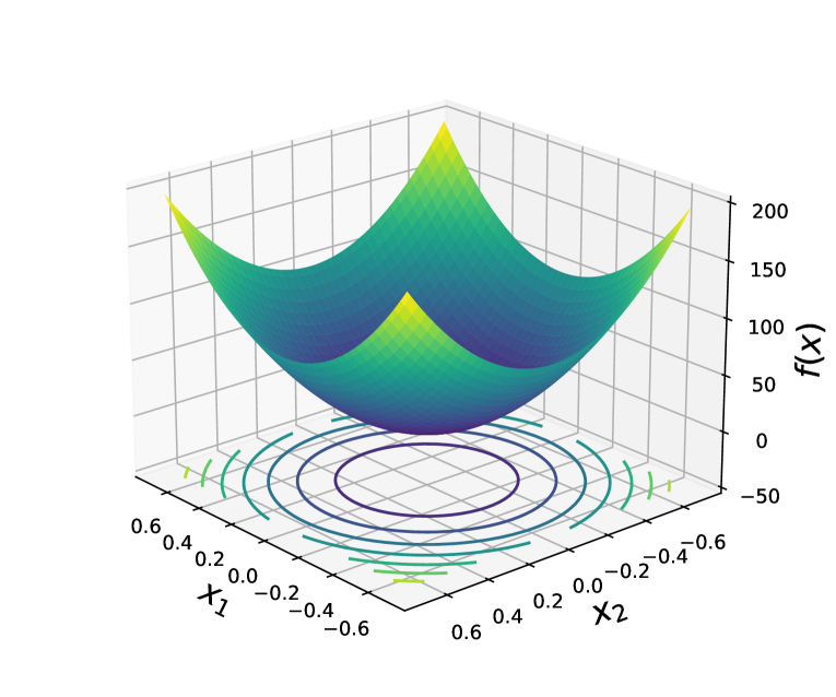
(a) Positive definite matrix: $\bm{A}=\scriptsize\begin{bmatrix}200&0\\ 0&200\end{bmatrix}$.

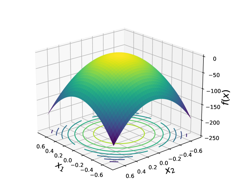
(b) Negative definite matrix: $\bm{A}=\scriptsize\begin{bmatrix}-200&0\\ 0&-200\end{bmatrix}$.

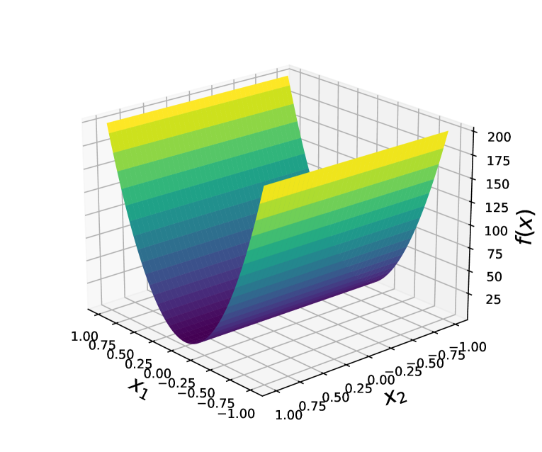
(c) Semidefinite matrix: $\bm{A}=\scriptsize\begin{bmatrix}200&0\\ 0&0\end{bmatrix}$. A line runs through the bottom of the valley is the set of solutions.

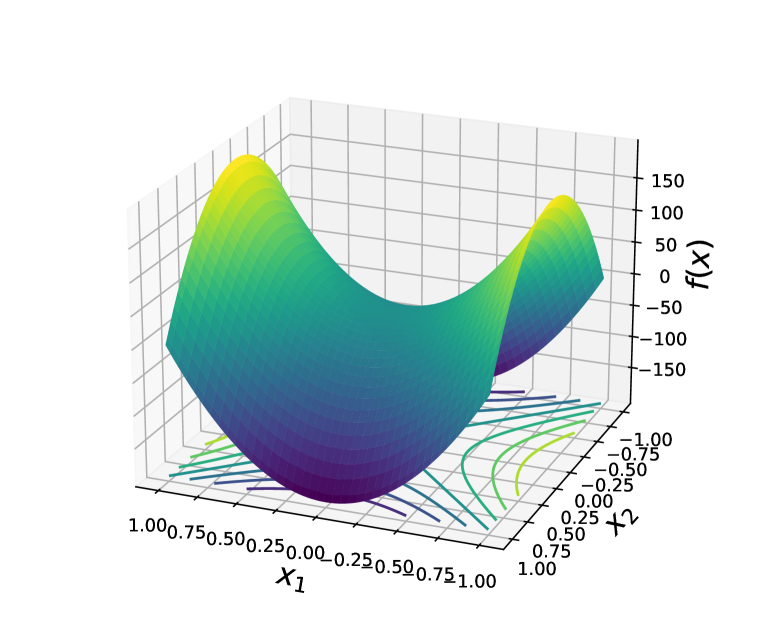
(d) Indefinte matrix: $\bm{A}=\scriptsize\begin{bmatrix}200&0\\ 0&-200\end{bmatrix}$.

Figure 1.4: Loss surfaces for different quadratic forms, providing the surface plots and contour plots (blue=low, yellow=high), where the upper graphs are the surface plots, and the lower ones are their projection (i.e., contours).

We further discuss linear systems with different types of matrices, the quadratic form:

$$f(\bm{x})=\frac{1}{2}\bm{x}^{\top}\bm{A}\bm{x}-\bm{b}^{\top}\bm{x}+c,\,\,\,\,\,\,\,\,\bm{x}\in^{n},$$ (1.21)

where $\bm{A}\in^{n\times n}$, $\bm{b}\in^{n}$, and $c$ is a scalar constant. Though the quadratic form in Equation (1.21) is an extremely simple model, it is rich enough to approximate many other functions, e.g., the Fisher information matrix (amari1998natural), and it captures key features of pathological curvature. The gradient of $f(\bm{x})$ at point $\bm{x}$ is given by

$$\nabla f(\bm{x})=\frac{1}{2}(\bm{A}^{\top}+\bm{A})\bm{x}-\bm{b}.$$

Any optimum point of the function is the solution to the linear system $\frac{1}{2}(\bm{A}^{\top}+\bm{A})\bm{x}=\bm{b}$:

$$\bm{x}^{*}=2(\bm{A}^{\top}+\bm{A})^{-1}\bm{b}.$$

If $\bm{A}$ is symmetric, the equation reduces to $\nabla f(\bm{x})=\bm{A}\bm{x}-\bm{b}.$ Then the optimum point of the function is the solution of the linear system $\bm{A}\bm{x}=\bm{b}$, where $\bm{A}$ and $\bm{b}$ are known matrix or vector, and $\bm{x}$ is an unknown vector; and the optimum point of $\bm{x}$ is thus given by

$$\bm{x}^{*}=\bm{A}^{-1}\bm{b},\quad\text{if $\bm{A}$ is nonsingular.}$$

For different types of matrix $\bm{A}$, the loss surface of $f(\bm{x})$ will vary as shown in Figure 1.4. When $\bm{A}$ is positive definite, the surface is a convex bowl; when $\bm{A}$ is negative definite, on the contrary, the surface is a concave bowl. $\bm{A}$ also could be singular, in which case $\bm{A}\bm{x}-\bm{b}=\mathbf{0}$ has more than one solution, and the set of solutions is a line (in the two-dimensional case) or a hyperplane (in the high-dimensional case). This situation is similar to the case of a semidefinite quadratic form, as shown in Figure 1.4(c). Moreover, $\bm{A}$ could be none of the above, then there exists a saddle point (see Figure 1.4(d)), where the gradient descent may fail (see discussions in the following chapters). In such senses, other methods, e.g., perturbed gradient descent (jin2017escape), can be applied to escape saddle points.

Diagonally dominant matrices.

A specific form of diagonally dominant matrices constitutes a significant subset of positive semidefinite matrices.

Definition 1.60 (Diagonally Dominant Matrices)

Given a symmetric matrix $\bm{A}\in^{n\times n}$, $\bm{A}$ is called diagonally dominant if

$$\left\lvert a_{ii}\right\rvert\geq\sum_{j\neq i}\left\lvert a_{ij}\right\rvert,\qquad\forall\,i\in\{1,2,\ldots,n\};$$

and $\bm{A}$ is called strictly diagonally dominant if

$$\left\lvert a_{ii}\right\rvert>\sum_{j\neq i}\left\lvert a_{ij}\right\rvert,\qquad\forall\,i\in\{1,2,\ldots,n\}.$$

We now show that diagonally dominant matrices with nonnegative diagonal elements are positive semidefinite and that strictly diagonally dominant matrices with positive diagonal elements are positive definite.

Given a symmetric matrix $\bm{A}\in^{n\times n}$, 1. If $\bm{A}$ is diagonally dominant with nonnegative diagonals, then $\bm{A}$ is positive semidefinite; 2. If $\bm{A}$ is strictly diagonally dominant with positive diagonals, then $\bm{A}$ is positive definite.

Proof [of Theorem 1.4.3] (i). Suppose $\bm{A}$ is not PSD and has a negative eigenvalue $\lambda$ associated with an eigenvector $\bm{v}$ such that $\bm{A}\bm{v}=\lambda\bm{v}$. Let $v_{i}$ be the element of $\bm{v}$ with largest magnitude. Consider the $i$-th element of $(\bm{A}-\lambda\bm{I})\bm{v}=\mathbf{0}$, we have

$$\left\lvert a_{ii}-\lambda\right\rvert\cdot\left\lvert v_{i}\right\rvert=\left\lvert\sum_{j\neq i}a_{ij}v_{j}\right\rvert\leq\left(\sum_{j\neq i}\left\lvert a_{ij}\right\rvert\right)\left\lvert v_{i}\right\rvert\leq\left\lvert a_{ij}\right\rvert\cdot\left\lvert v_{i}\right\rvert.$$

This implies $\left\lvert a_{ii}-\lambda\right\rvert\leq\left\lvert a_{ij}\right\rvert$ and leads to a contradiction.

(ii).

From part (i), we known that $\bm{A}$ is positive semidefinite. Suppose $\bm{A}$ is not positive definite and has a zero eigenvalue $0$ associated with a nonzero eigenvector $\bm{v}$ such that $\bm{A}\bm{v}=\mathbf{0}$. Similarly, we have

$$\left\lvert a_{ii}\right\rvert\cdot\left\lvert v_{i}\right\rvert=\left\lvert\sum_{j\neq i}a_{ij}v_{j}\right\rvert\leq\left(\sum_{j\neq i}\left\lvert a_{ij}\right\rvert\right)\left\lvert v_{i}\right\rvert<\left\lvert a_{ij}\right\rvert\cdot\left\lvert v_{i}\right\rvert,$$

which is impossible and the result follows.  

Exercise 1.62 (Quadratic Form)

Consider the quadratic form $f(\bm{x})=\frac{1}{2}\bm{x}^{\top}\bm{A}\bm{x}-\bm{b}^{\top}\bm{x}+c$, where $\bm{A}\in^{n\times n}$ is symmetric, $\bm{x}\in^{n}$, and $c\in$. Show that the following two claims are equivalent :

• $f(\bm{x})\geq 0$ for all $\bm{x}\in^{n}$.

• $\scriptsize\begin{bmatrix}\bm{A}&-\bm{b}\\ -\bm{b}^{\top}&2c\end{bmatrix}\succeq\mathbf{0}$.

Hint: Apply the eigenvalue characterization theorem on $\bm{A}$.

1.5 Differentiability and Differential Calculus

Definition 1.63 (Directional Derivative, Partial Derivative)

Given a function $f$ defined over a set ${\mathbb{S}}\subseteq^{n}$ and a nonzero vector $\bm{d}\in^{n}$, the directional derivative of $f$ at $\bm{x}$ with respect to the direction $\bm{d}$ is given by, if the limit exists,

$$\mathop{\lim}_{\mu\rightarrow 0}\frac{f(\bm{x}+\mu\bm{d})-f(\bm{x})}{\mu}.$$

And it is denoted by $f^{\prime}(\bm{x};\bm{d})$ or $D_{\bm{d}}f(\bm{x})$. The directional derivative is sometimes referred to as the Gâteaux derivative.

For any $i\in\{1,2,\ldots,n\}$, the directional derivative at $\bm{x}$ with respect to the direction of the $i$-th standard basis vector $\bm{e}_{i}$ (if it exists) is called the $i$-th partial derivative and is denoted by $\frac{\partial f}{\partial x_{i}}(\bm{x})$, $D_{\bm{e}_{i}}f(\bm{x})$, or $\partial_{i}f(\bm{x})$.

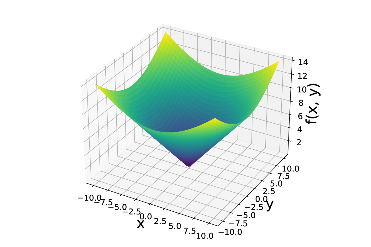
Figure 1.5: Plot for the function $f(x,y)=\sqrt{x^{2}+y^{2}}$, in which case any directional derivative for the direction $\bm{d}=[a,b]^{\top}$ with $a\neq 0$ and $b\neq 0$ at point $[0,0]^{\top}$ exists. However, the partial derivatives at this point do not exist.

It’s important to note that even if a function can have a directional derivative in every direction $\bm{d}$ at some points, its partial derivatives may not exist. For example, given the direction $\bm{d}=[a,b]^{\top}$ with $a\neq 0$ and $b\neq 0$, the directional derivation of the function $f(x,y)=\sqrt{x^{2}+y^{2}}$ (see Figure 1.5) at $[0,0]^{\top}$ can be obtained by

$$f^{\prime}(0,0;\bm{d})=\mathop{\lim}_{\mu\rightarrow 0}\frac{\sqrt{(0+\mu a)^{2}+(0+\mu b)^{2}}-\sqrt{0^{2}+0^{2}}}{\mu}=\sqrt{a^{2}+b^{2}}.$$

When $\bm{d}$ is a unit vector, the directional derivative is 1. However, it can be shown that the partial derivatives are

$$\frac{\partial f}{\partial x}(0,0) =\mathop{\lim}_{h\rightarrow 0}\frac{\sqrt{(0+h)^{2}+0^{2}}}{h}=\mathop{\lim}_{h\rightarrow 0}\frac{\left\lvert h\right\rvert}{h},$$

$$\frac{\partial f}{\partial y}(0,0) =\mathop{\lim}_{h\rightarrow 0}\frac{\sqrt{0^{2}+(0+h)^{2}}}{h}=\mathop{\lim}_{h\rightarrow 0}\frac{\left\lvert h\right\rvert}{h}.$$

When $h>0$, the partial derivatives are 1; when $h<0$, the partial derivaties are $-1$. Therefore, the partial derivatives do not exist.

If all the partial derivatives of a function $f$ exist at a point $\bm{x}\in^{n}$, then the gradient of $f$ at $\bm{x}$ is defined as the column vector containing all the partial derivatives:

$$\nabla f(\bm{x})=\begin{bmatrix}\frac{\partial f}{\partial x_{1}}(\bm{x}),\frac{\partial f}{\partial x_{2}}(\bm{x}),\ldots,\frac{\partial f}{\partial x_{n}}(\bm{x})\end{bmatrix}^{\top}\in^{n}.$$

Exercise 1.64

Show that a function can have partial derivatives but is not necessarily continuous (Definition 2.5). Additionally, demonstrate that a function can be continuous but does not necessarily have partial derivatives.

A function $f$ defined over an open set ${\mathbb{S}}\subseteq^{n}$ (Definition 2.4) is called differentiable if all its partial derivatives exist (i.e., the derivatives exist in univariate cases, and the gradients exist in multivariate cases). This is actually the definition of Fréchet differentiability.

Definition 1.65 ((Fréchet) Differentiability)

Given a function $f:^{n}\rightarrow$, the function $f$ is said to be differentiable at $\bm{x}$ if there exists a vector $\bm{g}\in^{n}$ such that

$$\mathop{\lim}_{\bm{d}\rightarrow\mathbf{0}}\frac{f(\bm{x}+\bm{d})-f(\bm{x})-\bm{g}^{\top}\bm{d}}{\left\lVert\bm{d}\right\rVert_{2}}=0.$$

The unique vector $\bm{g}$ is equal to the gradient $\nabla f(\bm{x})$.

Moreover, a function $f$ defined over an open set ${\mathbb{S}}\subseteq^{n}$ is called continuously differentiable over ${\mathbb{S}}$ if all its partial derivatives exist and are also continuous on ${\mathbb{S}}$.

A differentiable function may not be continuously differentiable. For example, consider the following function $f$:

$$f(x)=\begin{cases}x^{2}\sin(\frac{1}{x}),&\text{if }x\neq 0,\\ 0,&\text{if }x=0.\end{cases}$$

This function is differentiable everywhere, including at $x=0$. To see this, for $x\neq 0$, $f(x)$ is a product of two differentiable functions ($x^{2}$ and $\sin(1/x)$), hence it is differentiable. At $x=0$, we can calculate the derivative using the limit definition:

$$f^{\prime}(0)=\mathop{\lim}_{\mu\rightarrow 0}\frac{f(\mu)-f(0)}{\mu}=\mathop{\lim}_{\mu\rightarrow 0}\frac{\mu^{2}\sin(\frac{1}{\mu})-0}{\mu}=\mu\sin(\frac{1}{\mu})$$

Since $\left\lvert\sin(1/\mu)\right\rvert\leq 1$ for all $\mu\neq 0$, the limit exists and is equal to 0. Thus, $f(x)$ is differentiable at $x=0$ with $f^{\prime}(0)=0$. However, $f(x)$ is not continuously differentiable at $x=0$. The derivative of $f(x)$ when $x\neq 0$ is

$$f^{\prime}(x)=2x\sin(\frac{1}{x})-\cos(\frac{1}{x}).$$

The limit $\mathop{\lim}_{x\rightarrow 0}f^{\prime}(x)$ does not exist because the sine and cosine functions oscillate as $x$ approaches 0.

In the setting of differentiability, the directional derivative and gradient have the following relationship:

$$f^{\prime}(\bm{x};\bm{d})=\nabla f(\bm{x})^{\top}\bm{d},\,\,\,\,\,\,\,\,\text{for all }\bm{x}\in{\mathbb{S}}\text{ and }\bm{d}\in^{n}.$$ (1.22)

Proof  The formula is obviously correct for $\bm{d}=\mathbf{0}$. We then assume that $\bm{d}\neq\mathbf{0}$. The differentiability of $f$ implies that

$$0=\lim_{\mu\to 0^{+}}\frac{f(\bm{x}+\mu\bm{d})-f(\bm{x})-\langle\nabla f(\bm{x}),\mu\bm{d}\rangle}{\left\lVert\mu\bm{d}\right\rVert_{2}}=\lim_{\mu\to 0^{+}}\left[\frac{f(\bm{x}+\mu\bm{d})-f(\bm{x})}{\mu\left\lVert\bm{d}\right\rVert_{2}}-\frac{\langle\nabla f(\bm{x}),\bm{d}\rangle}{\left\lVert\bm{d}\right\rVert_{2}}\right].$$

Therefore,

$$f^{\prime}(\bm{x};\bm{d})=\lim_{\mu\to 0^{+}}\frac{f(\bm{x}+\mu\bm{d})-f(\bm{x})}{\mu}$$

$$=\lim_{\mu\to 0^{+}}\left\{\left\lVert\bm{d}\right\rVert_{2}\left[\frac{f(\bm{x}+\mu\bm{d})-f(\bm{x})}{\mu\left\lVert\bm{d}\right\rVert_{2}}-\frac{\langle\nabla f(\bm{x}),\bm{d}\rangle}{\left\lVert\bm{d}\right\rVert_{2}}\right]+\langle\nabla f(\bm{x}),\bm{d}\rangle\right\} =\langle\nabla f(\bm{x}),\bm{d}\rangle.$$

This proves (1.22).  

Recalling the definition of differentiability, we also have:

$$\mathop{\lim}_{\bm{d}\rightarrow\mathbf{0}}\frac{f(\bm{x}+\bm{d})-f(\bm{x})-\nabla f(\bm{x})^{\top}\bm{d}}{\left\lVert\bm{d}\right\rVert_{2}}=0\,\,\,\,\,\,\,\,\text{for all }\bm{x}\in{\mathbb{S}},$$ (1.23)

or

$$f(\bm{y})=f(\bm{x})+\nabla f(\bm{x})^{\top}(\bm{y}-\bm{x})+o(\left\lVert\bm{y}-\bm{x}\right\rVert_{2}),$$ (1.24)

where the small-oh function $o(\cdot):_{+}\rightarrow$ is a one-dimensional function satisfying $\frac{o(\mu)}{\mu}\rightarrow 0$ as $\mu\rightarrow 0^{+}$.  Therefore, any differentiable function ensures that $\mathop{\lim}_{\bm{x}\rightarrow\bm{a}}f(\bm{x})=f(\bm{a})$. Hence, any differentiable function is continuous.

On the other hand, in the setting of differentiability, although the partial derivatives may not be continuous, the partial derivatives exist for all differentiable points.

The partial derivative $\frac{\partial f}{\partial x_{i}}(\bm{x})$ is also a real-valued function of $\bm{x}\in{\mathbb{S}}$ that can be partially differentiated. The $j$-th partial derivative of $\frac{\partial f}{\partial x_{i}}(\bm{x})$ is defined as

$$\frac{\partial^{2}f}{\partial x_{j}\partial x_{i}}(\bm{x})=\frac{\partial\left(\frac{\partial f}{\partial x_{i}}(\bm{x})\right)}{\partial x_{j}}(\bm{x}).$$

This is called the ($j,i$)-th second-order partial derivative of function $f$. A function $f$ defined over an open set ${\mathbb{S}}\subseteq$ is called twice continuously differentiable over ${\mathbb{S}}$ if all the second-order partial derivatives exist and are continuous over ${\mathbb{S}}$. In the setting of twice continuously differentiability, the second-order partial derivative are symmetric:

$$\frac{\partial^{2}f}{\partial x_{j}\partial x_{i}}(\bm{x})=\frac{\partial^{2}f}{\partial x_{i}\partial x_{j}}(\bm{x}).$$

The Hessian of the function $f$ at a point $\bm{x}\in{\mathbb{S}}$ is defined as the symmetric $n\times n$ matrix

$$\nabla^{2}f(\bm{x})=\begin{bmatrix}\frac{\partial^{2}f}{\partial x_{1}^{2}}(\bm{x})&\frac{\partial^{2}f}{\partial x_{1}\partial x_{2}}(\bm{x})&\ldots&\frac{\partial^{2}f}{\partial x_{1}\partial x_{n}}(\bm{x})\\ \frac{\partial^{2}f}{\partial x_{2}\partial x_{1}}(\bm{x})&\frac{\partial^{2}f}{\partial x_{2}\partial x_{2}}(\bm{x})&\ldots&\frac{\partial^{2}f}{\partial x_{2}\partial x_{n}}(\bm{x})\\ \vdots&\vdots&\ddots&\vdots\\ \frac{\partial^{2}f}{\partial x_{n}\partial x_{1}}(\bm{x})&\frac{\partial^{2}f}{\partial x_{n}\partial x_{2}}(\bm{x})&\ldots&\frac{\partial^{2}f}{\partial x_{n}^{2}}(\bm{x})\end{bmatrix}.$$

We then provide a simple proof of Taylor’s expansion for one-dimensional functions. Let $f(x):\rightarrow$ be $k$-times continuously differentiable on the closed interval $I$ with endpoints $x$ and $y$, for some $k\geq 0$. If $f^{(k+1)}$ exists on the interval $I$, then there exists a $\xi\in(x,y)$ such that $\displaystyle f(x)$ $\displaystyle=f(y)+f^{\prime}(y)(x-y)+\ldots+\frac{f^{(k)}(y)}{k!}(x-y)^{k}+\frac{f^{(k+1)}(\xi)}{(k+1)!}(x-y)^{k+1}$ $\displaystyle=\sum_{i=0}^{k}\frac{f^{(i)}(y)}{i!}(x-y)^{i}+\frac{f^{(k+1)}(\xi)}{(k+1)!}(x-y)^{k+1}.$ Taylor’s expansion can be extended to a function of vector $f(\bm{x}):^{n}\rightarrow$ or a function of matrix $f(\bm{X}):^{m\times n}\rightarrow$. Taylor’s expansion, or also known as Taylor’s series, approximates the function $f(x)$ around a value $y$ using a polynomial in a single variable $x$. To understand the origin of this series, we recall from the elementary calculus course that the approximated function of $\cos(\theta)$ around $\theta=0$ is given by $\cos(\theta)\approx 1-\frac{\theta^{2}}{2}.$ This means that $\cos(\theta)$ can be approximated by a second-degree polynomial. If we want to approximate $\cos(\theta)$ more generally with a second-degree polynomial $f(\theta)=c_{1}+c_{2}\theta+c_{3}\theta^{2}$, an intuitive approach is to match the function and its derivatives at $\theta=0$. That is,

$$\left\{\begin{aligned} \cos(0)&=f(0);\\ \cos^{\prime}(0)&=f^{\prime}(0);\\ \cos^{\prime\prime}(0)&=f^{\prime\prime}(0);\\ \end{aligned}\right.\quad\implies\quad\left\{\begin{aligned} 1&=c_{1};\\ -\sin(0)&=0=c_{2};\\ -\cos(0)&=-1=2c_{3}.\\ \end{aligned}\right.$$

Solving these equations yields $f(\theta)=c_{1}+c_{2}\theta+c_{3}\theta^{2}=1-\frac{\theta^{2}}{2}$, which matches our initial approximation $\cos(\theta)\approx 1-\frac{\theta^{2}}{2}$ around $\theta=0$.

For high-dimensional functions, we have the following approximation results. Let $f(\bm{x}):{\mathbb{S}}\rightarrow$ be a continuously differentiable function over an open set ${\mathbb{S}}\subseteq^{n}$, and given two points $\bm{x},\bm{y}\in{\mathbb{S}}$. Then, there exists a point $\boldsymbol{\xi}\in[\bm{x},\bm{y}]$ such that $$f(\bm{y})=f(\bm{x})+\nabla f(\boldsymbol{\xi})^{\top}(\bm{y}-\bm{x}).$$

Let $f(\bm{x}):{\mathbb{S}}\rightarrow$ be a twice continuously differentiable function over an open set ${\mathbb{S}}\subseteq^{n}$, and let $\bm{x},\bm{y}\in{\mathbb{S}}$. Then, there exists a point $\boldsymbol{\xi}\in[\bm{x},\bm{y}]$ such that $$f(\bm{y})=f(\bm{x})+\nabla f(\bm{x})^{\top}(\bm{y}-\bm{x})+\frac{1}{2}(\bm{y}-\bm{x})^{\top}\nabla^{2}f(\boldsymbol{\xi})(\bm{y}-\bm{x}),$$ or $$f(\bm{y})=f(\bm{x})+\nabla f(\bm{x})^{\top}(\bm{y}-\bm{x})+o(\left\lVert\bm{y}-\bm{x}\right\rVert_{2}),$$ or $$f(\bm{y})=f(\bm{x})+\nabla f(\bm{x})^{\top}(\bm{y}-\bm{x})+\mathcal{O}(\left\lVert\bm{y}-\bm{x}\right\rVert_{2}^{2}).$$

Let $f(\bm{x}):{\mathbb{S}}\rightarrow$ be a twice continuously differentiable function over an open set ${\mathbb{S}}\subseteq^{n}$, and let $\bm{x},\bm{y}\in{\mathbb{S}}$. Then it follows that $$f(\bm{y})=f(\bm{x})+\nabla f(\bm{x})^{\top}(\bm{y}-\bm{x})+\frac{1}{2}(\bm{y}-\bm{x})^{\top}\nabla^{2}f(\bm{x})(\bm{y}-\bm{x})+o(\left\lVert\bm{y}-\bm{x}\right\rVert_{2}^{2}),$$ or $$f(\bm{y})=f(\bm{x})+\nabla f(\bm{x})^{\top}(\bm{y}-\bm{x})+\frac{1}{2}(\bm{y}-\bm{x})^{\top}\nabla^{2}f(\bm{x})(\bm{y}-\bm{x})+\mathcal{O}(\left\lVert\bm{y}-\bm{x}\right\rVert_{2}^{3}).$$

1.6 Fundamental Theorems

This section introduces fundamental theorems from optimization, linear algebra, and calculus that are frequently utilized in subsequent discussions. Let $\bm{a},\bm{b}\in^{n}$ be two vectors. The inner product of these two vectors can be expressed as a sum of norms: $$\bm{a}^{\top}\bm{b}=\frac{1}{2}\left(\left\lVert\bm{a}\right\rVert_{2}^{2}+\left\lVert\bm{b}\right\rVert_{2}^{2}-\left\lVert\bm{a}-\bm{b}\right\rVert_{2}^{2}\right).$$

The following theorem provides an elementary proof that the row rank and column rank of any matrix $\bm{A}\in^{m\times n}$ are equal, which also highlights the fundamental theorem of linear algebra. The dimension of the column space of a matrix $\bm{A}\in^{m\times n}$ is equal to the dimension of its row space. In other words, the row rank and the column rank of a matrix $\bm{A}$ are identical.

Proof [of Theorem 1.6] Firstly, observe that the null space of $\bm{A}$ is orthogonal complementary to the row space of $\bm{A}$: $\mathcal{N}(\bm{A})\bot\mathcal{C}(\bm{A}^{\top})$ (where the row space of $\bm{A}$ corresponds to the column space of $\bm{A}^{\top}$). This means that any vector in the null space of $\bm{A}$ is orthogonal to every vector in the row space of $\bm{A}$. To illustrate this, assume $\bm{A}$ has rows $\bm{a}_{1}^{\top},\bm{a}_{2}^{\top},\ldots,\bm{a}_{m}^{\top}$ and let $\bm{A}=[\bm{a}_{1}^{\top};\bm{a}_{2}^{\top};\ldots;\bm{a}_{m}^{\top}]$. For any vector $\bm{x}\in\mathcal{N}(\bm{A})$, we have $\bm{A}\bm{x}=\mathbf{0}$, implying $[\bm{a}_{1}^{\top}\bm{x};\bm{a}_{2}^{\top}\bm{x};\ldots;\bm{a}_{m}^{\top}\bm{x}]=\mathbf{0}$. And since the row space of $\bm{A}$ is spanned by $\bm{a}_{1}^{\top},\bm{a}_{2}^{\top},\ldots,\bm{a}_{m}^{\top}$, it follows that $\bm{x}$ is perpendicular to all vectors in $\mathcal{C}(\bm{A}^{\top})$, confirming $\mathcal{N}(\bm{A})\bot\mathcal{C}(\bm{A}^{\top})$.

Next, suppose the dimension of the row space of $\bm{A}$ is $r$. Let $\bm{r}_{1},\bm{r}_{2},\ldots,\bm{r}_{r}\in^{n}$ be a basis for the row space. Consequently, the $r$ vectors $\bm{A}\bm{r}_{1},\bm{A}\bm{r}_{2},\ldots,\bm{A}\bm{r}_{r}$ are in the column space of $\bm{A}$ and are linearly independent. To see this, suppose we have a linear combination of the $r$ vectors: $x_{1}\bm{A}\bm{r}_{1}+x_{2}\bm{A}\bm{r}_{2}+\ldots+x_{r}\bm{A}\bm{r}_{r}=\mathbf{0}$, that is, $\bm{A}(x_{1}\bm{r}_{1}+x_{2}\bm{r}_{2}+\ldots+x_{r}\bm{r}_{r})=\mathbf{0}$, and the vector $\bm{v}\triangleq x_{1}\bm{r}_{1}+x_{2}\bm{r}_{2}+\ldots+x_{r}\bm{r}_{r}$ is in null space of $\bm{A}$. But since $\{\bm{r}_{1},\bm{r}_{2},\ldots,\bm{r}_{r}\}$ is a basis for the row space of $\bm{A}$, $\bm{v}$ must also lie in the row space of $\bm{A}$. We have shown that vectors from the null space of $\bm{A}$ are perpendicular to vectors from the row space of $\bm{A}$; thus, it holds that $\bm{v}^{\top}\bm{v}=0$ and $x_{1}=x_{2}=\ldots=x_{r}=0$. Therefore, $\bm{A}\bm{r}_{1},\bm{A}\bm{r}_{2},\ldots,\bm{A}\bm{r}_{r}$ are in the column space of $\bm{A}$, and they are linearly independent. This implies that the dimension of the column space of $\bm{A}$ is larger than $r$. Therefore, the row rank of $\bm{A}\leq$ column rank of $\bm{A}$.

By applying the same argument to $\bm{A}^{\top}$, we deduce that column rank of $\bm{A}\leq$ row rank of $\bm{A}$, completing the proof that the row and column ranks of $\bm{A}$ are equal.  

From this proof, it follows that if $\{\bm{r}_{1},\bm{r}_{2},\ldots,\bm{r}_{r}\}$ is a set of vectors in ⁿ forming a basis for the row space, then $\{\bm{A}\bm{r}_{1},\bm{A}\bm{r}_{2},\ldots,\bm{A}\bm{r}_{r}\}$ constitutes a basis for the column space of $\bm{A}$. This observation is formalized in the following lemma.

Let $\bm{A}\in^{m\times n}$ be a matrix, and suppose that $\{\bm{r}_{1},\bm{r}_{2},\ldots,\bm{r}_{r}\}$ is a set of vectors in ⁿ, which forms a basis for the row space. Then, $\{\bm{A}\bm{r}_{1},\bm{A}\bm{r}_{2},\ldots,\bm{A}\bm{r}_{r}\}$ constitutes a basis for the column space of $\bm{A}$.

For any matrix $\bm{A}\in^{m\times n}$, it is straightforward to verify that any vector in the row space of $\bm{A}$ is orthogonal to any vector in the null space of $\bm{A}$. Suppose $\bm{x}_{n}\in\mathcal{N}(\bm{A})$, then $\bm{A}\bm{x}_{n}=\mathbf{0}$, meaning that $\bm{x}_{n}$ is orthogonal to every row of $\bm{A}$, thereby confirming this property.

Similarly, we can also demonstrate that any vector in the column space of $\bm{A}$ is perpendicular to any vector in the null space of $\bm{A}^{\top}$. Furthermore, the column space of $\bm{A}$ together with the null space of $\bm{A}^{\top}$ span the entire space ^m, which is a key aspect of the fundamental theorem of linear algebra.

The fundamental theorem consists of two aspects: the dimensions of the subspaces and their orthogonality. The orthogonality can be easily verified as shown above. Additionally, when the row space has dimension $r$, the null space has dimension $n-r$. This is not immediately obvious and is proven in the following theorem.

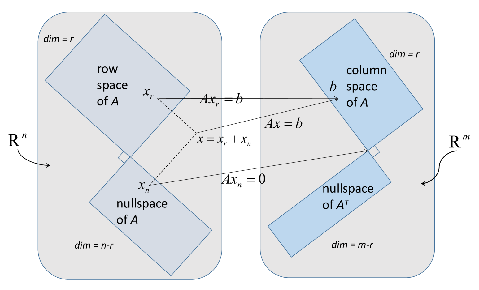
Figure 1.6: Two pairs of orthogonal subspaces in ⁿ and ^m. $\dim(\mathcal{C}(\bm{A}^{\top}))+\dim(\mathcal{N}(\bm{A}))=n$ and $\dim(\mathcal{N}(\bm{A}^{\top}))+\dim(\mathcal{C}(\bm{A}))=m$. The null space component maps to zero as $\bm{A}\bm{x}_{n}=\mathbf{0}\in^{m}$. The row space component maps to the column space as $\bm{A}\bm{x}_{r}=\bm{A}(\bm{x}_{r}+\bm{x}_{n})=\bm{b}\in\mathcal{C}(\bm{A})$.

Orthogonal Complement and Rank-Nullity Theorem: Let $\bm{A}\in^{m\times n}$ be a matrix. Then, $\mathcal{N}(\bm{A})$ is the orthogonal complement to the row space $\mathcal{C}(\bm{A}^{\top})$ in ⁿ: $\dim(\mathcal{N}(\bm{A}))+\dim(\mathcal{C}(\bm{A}^{\top}))=n$; $\mathcal{N}(\bm{A}^{\top})$ is the orthogonal complement to the column space $\mathcal{C}(\bm{A})$ in ^m: $\dim(\mathcal{N}(\bm{A}^{\top}))+\dim(\mathcal{C}(\bm{A}))=m$; If $\bm{A}$ has rank $r$, then $\dim(\mathcal{C}(\bm{A}^{\top}))=\dim(\mathcal{C}(\bm{A}))=r$, implying that $\dim(\mathcal{N}(\bm{A}))=n-r$ and $\dim(\mathcal{N}(\bm{A}^{\top}))=m-r$.

Proof [of Theorem 1.6] Building upon the proof of Theorem 1.6, consider a set of vectors $\bm{r}_{1},\bm{r}_{2},\ldots,\bm{r}_{r}$ in ⁿ forming a basis for the row space. Consequently, $\{\bm{A}\bm{r}_{1},\bm{A}\bm{r}_{2},\ldots,\bm{A}\bm{r}_{r}\}$ constitutes a basis for the column space of $\bm{A}$. Let $\bm{n}_{1},\bm{n}_{2},\ldots,\bm{n}_{k}\in^{n}$ form a basis for the null space of $\bm{A}$. Following again from the proof of Theorem 1.6, it follows that $\mathcal{N}(\bm{A})\bot\mathcal{C}(\bm{A}^{\top})$, indicating the orthogonality between $\bm{r}_{1},\bm{r}_{2},\ldots,\bm{r}_{r}$ and $\bm{n}_{1},\bm{n}_{2},\ldots,\bm{n}_{k}$. Consequently, the set $\{\bm{r}_{1},\bm{r}_{2},\ldots,\bm{r}_{r},\bm{n}_{1},\bm{n}_{2},\ldots,\bm{n}_{k}\}$ is linearly independent in ⁿ.

For any vector $\bm{x}\in^{n}$, $\bm{A}\bm{x}$ is in the column space of $\bm{A}$. Then it can be expressed as a linear combination of $\bm{A}\bm{r}_{1},\bm{A}\bm{r}_{2},\ldots,\bm{A}\bm{r}_{r}$: $\bm{A}\bm{x}\triangleq\sum_{i=1}^{r}a_{i}\bm{A}\bm{r}_{i}$, which states that $\bm{A}(\bm{x}-\sum_{i=1}^{r}a_{i}\bm{r}_{i})=\mathbf{0}$ and $\bm{x}-\sum_{i=1}^{r}a_{i}\bm{r}_{i}$ is thus in $\mathcal{N}(\bm{A})$. Since $\{\bm{n}_{1},\bm{n}_{2},\ldots,\bm{n}_{k}\}$ is a basis for the null space of $\bm{A}$, $\bm{x}-\sum_{i=1}^{r}a_{i}\bm{r}_{i}$ can be expressed as a linear combination of $\bm{n}_{1},\bm{n}_{2},\ldots,\bm{n}_{k}$: $\bm{x}-\sum_{i=1}^{r}a_{i}\bm{r}_{i}=\sum_{j=1}^{k}b_{j}\bm{n}_{j}$, i.e., $\bm{x}=\sum_{i=1}^{r}a_{i}\bm{r}_{i}+\sum_{j=1}^{k}b_{j}\bm{n}_{j}$. That is, any vector $\bm{x}\in^{n}$ can be expressed as $\{\bm{r}_{1},\bm{r}_{2},\ldots,\bm{r}_{r},\bm{n}_{1},\bm{n}_{2},\ldots,\bm{n}_{k}\}$ and the set forms a basis for ⁿ. Thus, the dimensions satisfy: $r+k=n$, i.e., $\dim(\mathcal{N}(\bm{A}))+\dim(\mathcal{C}(\bm{A}^{\top}))=n$. Similarly, we can prove that $\dim(\mathcal{N}(\bm{A}^{\top}))+\dim(\mathcal{C}(\bm{A}))=m$.  

Figure 1.6 visually represents the orthogonality of these subspaces and illustrates how $\bm{A}$ maps a vector $\bm{x}$ into the column space. The row space and null space dimensions add up to $n$, while the dimensions of the column space of $\bm{A}$ and the null space of $\bm{A}^{\top}$ sum to $m$. The null space component maps to zero as $\bm{A}\bm{x}_{\bm{n}}=\mathbf{0}\in^{m}$, which is the intersection of the column space of $\bm{A}$ and the null space of $\bm{A}^{\top}$. Conversely, the row space component transforms into the column space as $\bm{A}\bm{x}_{\bm{r}}=\bm{A}(\bm{x}_{\bm{r}}+\bm{x}_{\bm{n}})=\bm{b}\in^{m}$.

We provide the fundamental theorem of calculus below, which plays a pivotal role in linking differential and integral calculus, offering profound insights into the behavior of functions. Let $f(\cdot):^{n}\rightarrow$. The fundamental theorem of calculus describes the difference between function values: $$f(\bm{y})-f(\bm{x})=\int_{0}^{1}\langle\nabla f(\bm{x}+\mu(\bm{y}-\bm{x})),\bm{y}-\bm{x}\rangle d\mu,$$ (1.25a) or the difference between gradients: $\displaystyle\nabla f(\bm{y})-\nabla f(\bm{x})$ $\displaystyle=\left(\int_{0}^{1}\nabla^{2}f(\bm{x}+\mu(\bm{y}-\bm{x}))d\mu\right)\cdot(\bm{y}-\bm{x});$ (1.25b) $\displaystyle\nabla f(\bm{x}+\alpha\bm{d})-\nabla f(\bm{x})$ $\displaystyle=\int_{0}^{\alpha}\nabla^{2}f(\bm{x}+\mu\bm{d})\bm{d}d\mu.$ (1.25c) where $\nabla f(\bm{y})$ denotes the gradient of $f$ evaluated at $\bm{y}$ (see Section 1.5), and $\left\langle\cdot,\cdot\right\rangle$ represents the inner product. Furthermore, use directional derivative for twice continuously differentiable functions, we also have $$f(\bm{y})=f(\bm{x})+\left\langle\nabla f(\bm{x}),(\bm{y}-\bm{x})\right\rangle+\int_{0}^{1}(1-\mu)\frac{\partial^{2}f(\bm{x}+\mu(\bm{y}-\bm{x}))}{\partial\mu^{2}}d\mu.$$ (1.26) The first equality (1.25a) can be derived by letting $g(t)\triangleq f(\bm{x}+t(\bm{y}-\bm{x}))$. Then we can obtain $f(\bm{y})$ as $f(\bm{y})=g(1)=g(0)+\int_{0}^{1}g^{\prime}(t)dt.$ The other equalities can be demonstrated similarly.

We present the implicit function theorem without a proof. Further details can be found in krantz2002implicit. Let $\bm{h}(\bm{x})=[h_{i}(\bm{x})]_{i\in\{1,2,\ldots,p\}}:\mathbb{R}^{n}\rightarrow\mathbb{R}^{p}$ ($p<n$) and $\widetilde{\bm{x}}=[\widetilde{y}_{1},\ldots,\widetilde{y}_{p},\widetilde{z}_{1},\ldots,\widetilde{z}_{n-p}]=[\widetilde{\bm{y}},\widetilde{\bm{z}}]\in^{n}$ satisfy: 1. $\bm{h}(\widetilde{\bm{x}})=\mathbf{0}$. 2. $\bm{h}(\bm{x})$ is continuously differentiable in a neighborhood of $\widetilde{\bm{x}}$. 3. The $p\times p$ Jacobian matrix $$\small\begin{bmatrix}\frac{\partial h_{1}(\widetilde{\bm{x}})}{\partial y_{1}}&\cdots&\frac{\partial h_{1}(\widetilde{\bm{x}})}{\partial y_{p}}\\ \vdots&\ddots&\vdots\\ \frac{\partial h_{p}(\widetilde{\bm{x}})}{\partial y_{1}}&\cdots&\frac{\partial h_{p}(\widetilde{\bm{x}})}{\partial y_{p}}\end{bmatrix}$$ is nonsingular. Then, there exists $\varepsilon>0$ along with functions $\bm{s}(\bm{z})=[s_{1}(\bm{z}),\ldots,s_{p}(\bm{z})]^{\top}\in^{p}$ such that for all $\bm{z}\in{\mathbb{B}}(\widetilde{\bm{z}},\varepsilon)$, $\bm{h}(\bm{s}(\bm{z}),\bm{z})=\mathbf{0}$. Moreover, each $s_{k}(\bm{z})$ is continuously differentiable for $k\in\{1,2,\ldots,p\}$. Furthermore, for all $i\in\{1,2,\ldots,p\}$ and $j\in\{1,2,\ldots,n-p\}$, we have: $$\sum_{k=1}^{p}\frac{\partial h_{i}(\bm{y},\bm{z})}{\partial y_{k}}\frac{\partial s_{k}(\bm{z})}{\partial z_{j}}+\frac{\partial h_{i}(\bm{y},\bm{z})}{\partial z_{j}}=0.$$

Let $F:\mathbb{R}^{n}\to\mathbb{R}^{n}$ be a continuously differentiable function, and let $\bm{x}^{*}$ be a point in $\mathbb{R}^{n}$. If the derivative of $F$ at $\bm{x}^{*}$, denoted as $\nabla F(\bm{x}^{*})$, is an invertible linear transformation (meaning the Jacobian matrix $\bm{J}_{F}(\bm{x}^{*})$ is nonsingular), then there exists an open neighborhood ${\mathbb{S}}$ of $\bm{x}^{*}$ such that: 1. $F$ maps ${\mathbb{S}}$ bijectively onto an open set ${\mathbb{V}}=F({\mathbb{S}})$, 2. The inverse function $F^{-1}:{\mathbb{V}}\to{\mathbb{S}}$ is also continuously differentiable, 3. For each $\bm{y}\in{\mathbb{V}}$, the derivative of the inverse function at $\bm{y}$ is the inverse of the derivative of $F$ at $\bm{x}$, where $F(\bm{x})=\bm{y}$; i.e., $$\nabla(F^{-1})(\bm{y})=[\nabla F(\bm{x})]^{-1}.$$

In simpler terms, if a function locally behaves like a linear transformation (i.e., its derivative is nonzero and invertible), then near that point, an inverse function exists that “undoes” the original function. This inverse function is also smooth (continuously differentiable). The inverse function theorem is a powerful tool that has wide-ranging applications in mathematics, physics, economics, and engineering. For example, the theorem can be used to solve systems of nonlinear equations by transforming them into a system of linear equations.

Let $\left\lVert\cdot\right\rVert$ be a submultiplicative matrix norm with $\left\lVert\bm{I}\right\rVert=1$, and let $\bm{E}\in^{n\times n}$. If $\left\lVert\bm{E}\right\rVert<1$, then $\bm{I}-\bm{E}$ is nonsingular, and $$(\bm{I}-\bm{E})^{-1}=\sum_{t=0}^{\infty}\bm{E}^{t},$$ (1.27) $$\left\lVert(\bm{I}-\bm{E})^{-1}\right\rVert\leq\frac{1}{1-\left\lVert\bm{E}\right\rVert}.$$ (1.28) If $\bm{A}\in^{n\times n}$ is nonsingular and $\left\lVert\bm{A}^{-1}(\bm{B}-\bm{A})\right\rVert<1$, then $\bm{B}$ is nonsingular and satisfies $$\bm{B}^{-1}=\sum_{t=0}^{\infty}(\bm{I}-\bm{A}^{-1}\bm{B})^{t}\bm{A}^{-1},$$ (1.29) and $$\left\lVert\bm{B}^{-1}\right\rVert\leq\frac{\left\lVert\bm{A}^{-1}\right\rVert}{1-\left\lVert\bm{A}^{-1}(\bm{B}-\bm{A})\right\rVert}.$$ (1.30)

Proof [of Theorem 1.6] Since $\left\lVert\bm{E}\right\rVert<1$, then $\bm{S}_{t}\triangleq\bm{I}+\bm{E}+\bm{E}^{2}+\cdots+\bm{E}^{t}$ defines a Cauchy sequence and thus $\bm{S}_{t}$ converges. Taking the limit, we obtain $\sum_{t=0}^{\infty}\bm{E}^{t}=\lim_{t\to\infty}\bm{S}_{t}=(\bm{I}-\bm{E})^{-1}$ which proves (1.27) and (1.28). For the second part, since $\bm{A}$ is nonsingular and $\left\lVert\bm{A}^{-1}(\bm{B}-\bm{A})\right\rVert=\left\lVert-(\bm{I}-\bm{A}^{-1}\bm{B})\right\rVert<1$, we set $\bm{E}\triangleq\bm{I}-\bm{A}^{-1}\bm{B}$ and apply (1.27) and (1.28), immediately yielding (1.29) and (1.30).  

Let $F:{\mathbb{S}}\subset\mathbb{R}^{n}\to\mathbb{R}^{n}$ be continuously differentiable in a neighborhood of $\bm{x}^{*}\in{\mathbb{S}}$, and suppose that $\nabla F(\bm{x}^{*})$ is nonsingular. Then there exist $\delta>0$, $\xi>0$, and $\epsilon>0$, such that when $\left\lVert\bm{y}-\bm{x}^{*}\right\rVert_{2}<\delta$ and $\bm{y}\in{\mathbb{S}}$, $\nabla F(\bm{y})$ is nonsingular and $$\left\lVert\nabla F(\bm{y})^{-1}\right\rVert_{2}\leq\xi,$$ (1.31) where $\left\lVert\cdot\right\rVert_{2}$ for a matrix denotes the spectral norm. Additionally, the inverse $\nabla F(\bm{y})^{-1}$ is continuous at $\bm{x}^{*}$, meaning $$\left\lVert\nabla F(\bm{y})^{-1}-\nabla F(\bm{x}^{*})^{-1}\right\rVert_{2}<\epsilon.$$

Proof  Define $\alpha\triangleq\left\lVert\nabla F(\bm{x}^{*})^{-1}\right\rVert_{2}$. Since $F$ is continuously differentiable, for a given $\beta<\alpha^{-1}$, choose $\delta$ such that when $\left\lVert\bm{y}-\bm{x}^{*}\right\rVert_{2}<\delta$ with $\bm{y}\in{\mathbb{S}}$,

$$\left\lVert\nabla F(\bm{x}^{*})-\nabla F(\bm{y})\right\rVert_{2}\leq\beta.$$

It follows from Von-Neumann lemma (Theorem 1.6) that $\nabla F(\bm{y})$ is invertible, and (1.30) shows that

$$\left\lVert\nabla F(\bm{y})^{-1}\right\rVert_{2}\leq\frac{\left\lVert\nabla F(\bm{x}^{*})^{-1}\right\rVert_{2}}{1-\left\lVert\nabla F(\bm{x}^{*})^{-1}(\nabla F(\bm{y})-\nabla F(\bm{x}^{*}))\right\rVert_{2}}\leq\alpha/(1-\beta\alpha).$$

Therefore, (1.31) holds with $\xi\triangleq\alpha/(1-\beta\alpha)$. Thus,

$$\left\lVert\nabla F(\bm{x}^{*})^{-1}-\nabla F(\bm{y})^{-1}\right\rVert_{2} =\left\lVert\nabla F(\bm{x}^{*})^{-1}(\nabla F(\bm{y})-\nabla F(\bm{x}^{*}))\nabla F(\bm{y})^{-1}\right\rVert_{2}\leq\alpha\beta\xi\triangleq\epsilon,$$

which shows that the continuity of $\nabla F$ guarantees the continuity of $(\nabla F)^{-1}$.  

1.7 Matrix Decomposition

This section provide several matrix decomposition approaches, which can be useful for the proofs in the optimization methods.

1.7.1 Cholesky Decomposition

Positive definiteness or positive semidefiniteness is one of the most desirable properties a matrix can have. In this section, we introduce decomposition techniques for positive definite matrices, with a focus on the well-known Cholesky decomposition. The Cholesky decomposition is named after a French military officer and mathematician, André-Louis Cholesky (1875–1918), who developed this method in his surveying work. It is primarily used to solve linear systems involving positive definite matrices.

Here, we establish the existence of the Cholesky decomposition using an inductive approach. Alternative proofs also exist, such as those derived from the LU decomposition (lu2022matrix).

Every positive definite (PD) matrix $\bm{A}\in^{n\times n}$ can be factored as $$\bm{A}=\bm{R}^{\top}\bm{R},$$ where $\bm{R}\in^{n\times n}$ is an upper triangular matrix with positive diagonal elements. This decomposition is called the Cholesky decomposition of $\bm{A}$, and $\bm{R}$ is known as the Cholesky factor or Cholesky triangle of $\bm{A}$. Specifically, the Cholesky decomposition is unique (Corollary 1.7.1).

Alternatively, $\bm{A}$ can be factored as $\bm{A}=\bm{L}\bm{L}^{\top}$, where $\bm{L}=\bm{R}^{\top}$ is a lower triangular matrix with positive diagonals.

Proof [of Theorem 1.7.1] We will prove by induction that every $n\times n$ positive definite matrix $\bm{A}$ has a decomposition $\bm{A}=\bm{R}^{\top}\bm{R}$. The $1\times 1$ case is trivial by setting $R\triangleq\sqrt{A}$, so that $A=R^{2}$.

Suppose any $k\times k$ PD matrix $\bm{A}_{k}$ has a Cholesky decomposition. We must show that any $(k+1)\times(k+1)$ PD matrix $\bm{A}_{k+1}$ can also be factored as this Cholesky decomposition, then we complete the proof.

For any $(k+1)\times(k+1)$ PD matrix $\bm{A}_{k+1}$, write $\bm{A}_{k+1}$ as $\bm{A}_{k+1}\triangleq\footnotesize\begin{bmatrix}\bm{A}_{k}&\bm{b}\\ \bm{b}^{\top}&d\end{bmatrix}.$ Since $\bm{A}_{k}$ is PD, by the inductive hypothesis, it admits a Cholesky decomposition $\bm{A}_{k}=\bm{R}_{k}^{\top}\bm{R}_{k}$. Define the upper triangular matrix $\bm{R}_{k+1}\triangleq\footnotesize\begin{bmatrix}\bm{R}_{k}&\bm{r}\\ 0&s\end{bmatrix}.$ Then,

$$\bm{R}_{k+1}^{\top}\bm{R}_{k+1}=\begin{bmatrix}\bm{R}_{k}^{\top}\bm{R}_{k}&\bm{R}_{k}^{\top}\bm{r}\\ \bm{r}^{\top}\bm{R}_{k}&\bm{r}^{\top}\bm{r}+s^{2}\end{bmatrix}.$$

Therefore, if we can prove $\bm{R}_{k+1}^{\top}\bm{R}_{k+1}=\bm{A}_{k+1}$ is the Cholesky decomposition of $\bm{A}_{k+1}$ (which requires the value $s$ to be positive), then we complete the proof. That is, we need to prove

$$\bm{b} =\bm{R}_{k}^{\top}\bm{r},$$

$$d =\bm{r}^{\top}\bm{r}+s^{2}.$$

Since $\bm{R}_{k}$ is nonsingular, we can solve uniquely for $\bm{r}$ and $s$:

$$\bm{r} =\bm{R}_{k}^{-\top}\bm{b},$$

$$s =\sqrt{d-\bm{r}^{\top}\bm{r}}=\sqrt{d-\bm{b}^{\top}\bm{A}_{k}^{-1}\bm{b}},$$

where we assume $s$ is nonnegative. However, we need to further prove that $s$ is not only nonnegative, but also positive. Since $\bm{A}_{k}$ is PD, from Sylvester’s criterion (see lu2022matrix), and the fact that if matrix $\bm{M}$ has a block formulation: $\bm{M}=\footnotesize\begin{bmatrix}\bm{A}&\bm{B}\\ \bm{C}&\bm{D}\end{bmatrix}$, then $\det(\bm{M})=\det(\bm{A})\det(\bm{D}-\bm{C}\bm{A}^{-1}\bm{B})$, we have

$$\det(\bm{A}_{k+1})=\det(\bm{A}_{k})\det(d-\bm{b}^{\top}\bm{A}_{k}^{-1}\bm{b})=\det(\bm{A}_{k})(d-\bm{b}^{\top}\bm{A}_{k}^{-1}\bm{b})>0.$$

Because $\det(\bm{A}_{k})>0$, we then obtain that $(d-\bm{b}^{\top}\bm{A}_{k}^{-1}\bm{b})>0$, and this implies $s>0$. This completes the proof.  

The Cholesky decomposition $\bm{A}=\bm{R}^{\top}\bm{R}$ for any positive definite matrix $\bm{A}\in^{n\times n}$ is unique.

Proof [of Corollary 1.7.1] Suppose the Cholesky decomposition is not unique. Then, there exist two distinct decompositions such that $\bm{A}=\bm{R}_{1}^{\top}\bm{R}_{1}=\bm{R}_{2}^{\top}\bm{R}_{2}$. Rearranging, we obtain

$$\bm{R}_{1}\bm{R}_{2}^{-1}=\bm{R}_{1}^{-\top}\bm{R}_{2}^{\top}.$$

Since the inverse of an upper triangular matrix is also upper triangular, and the product of two upper triangular matrices is upper triangular, we conclude that the left-hand side of the above equation is an upper triangular matrix, while the right-hand side is a lower triangular matrix. Consequently, $\bm{R}_{1}\bm{R}_{2}^{-1}=\bm{R}_{1}^{-\top}\bm{R}_{2}^{\top}$ must be a diagonal matrix, and $\bm{R}_{1}^{-\top}\bm{R}_{2}^{\top}=(\bm{R}_{1}^{-\top}\bm{R}_{2}^{\top})^{\top}=\bm{R}_{2}\bm{R}_{1}^{-1}$. Let $\boldsymbol{\Lambda}\triangleq\bm{R}_{1}\bm{R}_{2}^{-1}=\bm{R}_{2}\bm{R}_{1}^{-1}$ be the diagonal matrix. We notice that the diagonal value of $\boldsymbol{\Lambda}$ is the product of the corresponding diagonal values of $\bm{R}_{1}$ and $\bm{R}_{2}^{-1}$ (or $\bm{R}_{2}$ and $\bm{R}_{1}^{-1}$). Explicitly, writing the matrices as

$$\bm{R}_{1}=\small\begin{bmatrix}r_{11}&r_{12}&\ldots&r_{1n}\\ 0&r_{22}&\ldots&r_{2n}\\ \vdots&\vdots&\ddots&\vdots\\ 0&0&\ldots&r_{nn}\end{bmatrix},\qquad\normalsize\bm{R}_{2}=\small\begin{bmatrix}s_{11}&s_{12}&\ldots&s_{1n}\\ 0&s_{22}&\ldots&s_{2n}\\ \vdots&\vdots&\ddots&\vdots\\ 0&0&\ldots&s_{nn}\end{bmatrix},$$

we find that

$$\bm{R}_{1}\bm{R}_{2}^{-1}=\small\begin{bmatrix}\frac{r_{11}}{s_{11}}&0&\ldots&0\\ 0&\frac{r_{22}}{s_{22}}&\ldots&0\\ \vdots&\vdots&\ddots&\vdots\\ 0&0&\ldots&\frac{r_{nn}}{s_{nn}}\end{bmatrix}=\small\begin{bmatrix}\frac{s_{11}}{r_{11}}&0&\ldots&0\\ 0&\frac{s_{22}}{r_{22}}&\ldots&0\\ \vdots&\vdots&\ddots&\vdots\\ 0&0&\ldots&\frac{s_{nn}}{r_{nn}}\end{bmatrix}\normalsize=\bm{R}_{2}\bm{R}_{1}^{-1}.$$

Since both $\bm{R}_{1}$ and $\bm{R}_{2}$ have positive diagonals, this implies $r_{11}=s_{11},r_{22}=s_{22},\ldots,r_{nn}=s_{nn}$. Thus, we conclude that $\boldsymbol{\Lambda}=\bm{R}_{1}\bm{R}_{2}^{-1}=\bm{R}_{2}\bm{R}_{1}^{-1}=\bm{I}$, which implies $\bm{R}_{1}=\bm{R}_{2}$, contradicting our initial assumption that the decomposition was not unique. Therefore, the Cholesky decomposition is unique.  

Computing Cholesky decomposition element-wise.

It is common to compute the Cholesky decomposition using element-wise equations derived directly from solving the matrix equation $\bm{A}=\bm{R}^{\top}\bm{R}$. Observing that the $(i,j)$-th entry of $\bm{A}$ is given by $a_{ij}=\bm{R}_{:,i}^{\top}\bm{R}_{:,j}=\sum_{k=1}^{i}r_{ki}r_{kj}$ if $i<j$. This further implies the following recurrence relation: if $i<j$, we have

$$a_{ij} =\bm{R}_{:,i}^{\top}\bm{R}_{:,j}=\sum_{k=1}^{i}r_{ki}r_{kj}=\sum_{k=1}^{i-1}r_{ki}r_{kj}+r_{ii}r_{ij}\implies r_{ij}=(a_{ij}-\sum_{k=1}^{i-1}r_{ki}r_{kj})/r_{ii},\,\,\,\,\,\,\,\,\text{if }i<j.$$

For the diagonal entries ($i=j$), we have:

$$a_{jj} =\sum_{k=1}^{j}r_{kj}^{2}=\sum_{k=1}^{j-1}r_{kj}^{2}+r_{jj}^{2} \implies r_{jj}=\sqrt{a_{jj}-\sum_{k=1}^{j-1}r_{kj}^{2}}.$$

If we equate the elements of $\bm{R}$ by taking a column at a time and start with $r_{11}=\sqrt{a_{11}}$, the element-level algorithm is formulated in Algorithm 1.

Algorithm 1 Cholesky Decomposition Element-Wise: $\bm{A}=\bm{R}^{\top}\bm{R}$

1:Positive definite matrix $\bm{A}$ with size $n\times n$;

2:Calculate first element of $\bm{R}$ by $r_{11}\leftarrow\sqrt{a_{11}}$;

3:for $j=1$ to $n$ do $\triangleright$ Compute the $j$-th column of $\bm{R}$

4:  for $i=1$ to $j-1$ do

5:   $r_{ij}\leftarrow(a_{ij}-\sum_{k=1}^{i-1}r_{ki}r_{kj})/r_{ii}$, since $i<j$;

6:  end for

7:  $r_{jj}\leftarrow\sqrt{a_{jj}-\sum_{k=1}^{j-1}r_{kj}^{2}}$;

8:end for

9:Output $\bm{A}=\bm{R}^{\top}\bm{R}$.

On the other hand, Algorithm 1 can be modified to compute the Cholesky decomposition in the form $\bm{A}=\bm{L}\bm{D}\bm{L}^{\top}$, where $\bm{L}$ is unit lower triangular and $\bm{D}$ is diagonal, as outlined in Algorithm 2, whose Step 3 and Step 5 are derived from (since $l_{ii}=1,\forall\,i\in\{1,2,\ldots,n\}$):

$$a_{jj} =\sum_{k=1}^{j-1}d_{kk}l_{jk}^{2}+d_{jj};$$

$$a_{ij} =d_{jj}l_{ij}+\sum_{k=1}^{j-1}d_{kk}l_{ik}l_{jk},\,\,\,\,\,\,\,\,\text{if }i>j.$$

Exercise 1.81

Derive the complexity of Algorithm 2.

This form of Cholesky decomposition is useful for determining the condition number of a PD matrix (lu2021numerical). In essence, the condition number of a function measures the sensitivity of the output value to small changes in the input; a smaller condition number indicates better numerical stability. For positive definite linear systems, the condition number is defined as the ratio of the largest eigenvalue to the smallest eigenvalue. The condition number of a positive definite matrix is lower bounded by the diagonal matrix in the Cholesky decomposition (see Problem 1.2.):

$$\text{cond}(\bm{A})\geq\text{cond}(\bm{D}).$$ (1.32)

This can be proven by showing that $\lambda_{\max}\geq d_{\max}$ and $\lambda_{\min}\leq d_{\min}$, where $\lambda_{\max}$ and $\lambda_{\min}$ are the largest and smallest eigenvalue of $\bm{A}$, and $d_{\max}$ and $d_{\min}$ are the largest and smallest diagonals of $\bm{D}$. Therefore, this form of the Cholesky decomposition can be utilized to modify Newton’s method; see § LABEL:section:modified_damp_new.

Algorithm 2 Cholesky Decomposition Element-Wise: $\bm{A}=\bm{L}\bm{D}\bm{L}^{\top}$

1:Positive definite matrix $\bm{A}$ with size $n\times n$;

2:for $j=1$ to $n$ do $\triangleright$ Compute the $j$-th column of $\bm{L}$

3:  $l_{jj}\leftarrow 1$;

4:  $c_{jj}\leftarrow a_{jj}-\sum_{k=1}^{j-1}d_{kk}l_{jk}^{2}$;

5:  $d_{jj}\leftarrow c_{jj}$

6:  for $i=j+1$ to $n$ do

7:   $c_{ij}\leftarrow a_{ij}-\sum_{k=1}^{j-1}d_{kk}l_{ik}l_{jk}$, since $i>j$;

8:   $l_{ij}\leftarrow\frac{c_{ij}}{d_{jj}}$;

9:  end for

10:end for

11:Output $\bm{A}=\bm{L}\bm{D}\bm{L}^{\top}$, where $\bm{D}=\mathrm{diag}(d_{11},d_{22},\ldots,d_{nn})$.

1.7.2 Eigenvalue and Spectral Decomposition

Eigenvalue decomposition is also known as to diagonalize the matrix. If a matrix $\bm{A}\in^{n\times n}$ has distinct eigenvalues, its corresponding eigenvectors are guaranteed to be linearly independent, allowing $\bm{A}$ to be diagonalized. It is important to note that without $n$ linearly independent eigenvectors, diagonalization is not possible. Any square matrix $\bm{A}\in^{n\times n}$ with linearly independent eigenvectors can be factored as $$\bm{A}=\bm{X}\boldsymbol{\Lambda}\bm{X}^{-1},$$ where $\bm{X}\in^{n\times n}$ is a matrix whose columns are the eigenvectors of $\bm{A}$, and $\boldsymbol{\Lambda}\in^{n\times n}$ is a diagonal matrix given by $\mathrm{diag}(\lambda_{1},$ $\lambda_{2},\ldots,\lambda_{n})$ with $\lambda_{1},\lambda_{2},\ldots,\lambda_{n}$ denoting the eigenvalues of $\bm{A}$.

Proof [of Theorem 1.7.2] Let $\bm{X}=[\bm{x}_{1},\bm{x}_{2},\ldots,\bm{x}_{n}]$ be the linearly independent eigenvectors of $\bm{A}$. Clearly, we have

$$\bm{A}\bm{x}_{1}=\lambda_{1}\bm{x}_{1},\qquad\bm{A}\bm{x}_{2}=\lambda_{2}\bm{x}_{2},\qquad\ldots,\qquad\bm{A}\bm{x}_{n}=\lambda_{n}\bm{x}_{n}.$$

Expressing this in matrix form, we obtain

$$\bm{A}\bm{X}=[\bm{A}\bm{x}_{1},\bm{A}\bm{x}_{2},\ldots,\bm{A}\bm{x}_{n}]=[\lambda_{1}\bm{x}_{1},\lambda_{2}\bm{x}_{2},\ldots,\lambda_{n}\bm{x}_{n}]=\bm{X}\boldsymbol{\Lambda}.$$

Since the eigenvectors are linearly independent, $\bm{X}$ is invertible, leading to $\bm{A}=\bm{X}\boldsymbol{\Lambda}\bm{X}^{-1}.$ This completes the proof.  

An important advantage of the decomposition $\bm{A}=\bm{X}\boldsymbol{\Lambda}\bm{X}^{-1}$ is that it allows efficient computation of matrix powers.

Remark 1.83 ($m$-th Power)

If $\bm{A}$ admits an eigenvalue decomposition $\bm{A}=\bm{X}\boldsymbol{\Lambda}\bm{X}^{-1}$, then its $m$-th power can be computed as $\bm{A}^{m}=\bm{X}\boldsymbol{\Lambda}^{m}\bm{X}^{-1}$.

The existence of eigenvalue decomposition depends on the linear independence of the eigenvectors of $\bm{A}$. This condition is automatically satisfied in specific cases. If the eigenvalues $\lambda_{1},\lambda_{2},\ldots,\lambda_{n}$ of $\bm{A}\in^{n\times n}$ are all distinct, then the associated eigenvectors are necessarily linearly independent. Consequently, any square matrix with unique eigenvalues is diagonalizable.

Proof [of Lemma 1.7.2] Assume that $\bm{A}$ has distinct eigenvalues $\lambda_{1},\lambda_{2},\ldots,\lambda_{n}$ and that the eigenvectors $\bm{x}_{1},\bm{x}_{2},\ldots,\bm{x}_{n}$ are linearly dependent. Then, there exists a nonzero vector $\bm{c}=[c_{1},c_{2},\ldots,c_{n-1}]^{\top}$ such that $\bm{x}_{n}=\sum_{i=1}^{n-1}c_{i}\bm{x}_{i}.$ Applying $\bm{A}$ to both sides, we get

$$\bm{A}\bm{x}_{n} =\bm{A}(\sum_{i=1}^{n-1}c_{i}\bm{x}_{i})=c_{1}\lambda_{1}\bm{x}_{1}+c_{2}\lambda_{2}\bm{x}_{2}+\ldots+c_{n-1}\lambda_{n-1}\bm{x}_{n-1}.$$

and

$$\bm{A}\bm{x}_{n} =\lambda_{n}\bm{x}_{n}=\lambda_{n}(c_{1}\bm{x}_{1}+c_{2}\bm{x}_{2}+\ldots+c_{n-1}\bm{x}_{n-1}).$$

Equating both expressions, we obtain $\sum_{i=1}^{n-1}(\lambda_{n}-\lambda_{i})c_{i}\bm{x}_{i}=\mathbf{0}.$ This leads to a contradiction since $\lambda_{n}\neq\lambda_{i}$ for all $i\in\{1,2,\ldots,n-1\}$, from which the result follows.  

The spectral theorem, also referred to as the spectral decomposition for symmetric matrices, states that every symmetric matrix has real eigenvalues and can be diagonalized using a (real) orthonormal basis . A real matrix $\bm{A}\in^{n\times n}$ is symmetric if and only if there exists an orthogonal matrix $\bm{Q}$ and a diagonal matrix $\boldsymbol{\Lambda}$ such that $$\bm{A}=\bm{Q}\boldsymbol{\Lambda}\bm{Q}^{\top},$$ (1.33) where the columns of $\bm{Q}=[\bm{q}_{1},\bm{q}_{2},\ldots,\bm{q}_{n}]$ are eigenvectors of $\bm{A}$ and are mutually orthonormal, and the entries of $\boldsymbol{\Lambda}=\mathrm{diag}(\lambda_{1},\lambda_{2},\ldots,\lambda_{n})$ are the corresponding real eigenvalues of $\bm{A}$. Moreover, the rank of $\bm{A}$ is equal to the number of nonzero eigenvalues. This result is known as the spectral decomposition or the spectral theorem for real symmetric matrices. Specifically, the following properties hold: 1. A symmetric matrix has only real eigenvalues. 2. The eigenvectors are orthogonal and can be chosen to be orthonormal by normalization. 3. The rank of $\bm{A}$ is equal to the number of nonzero eigenvalues (Proposition 1.4.1). 4. If the eigenvalues are distinct, the eigenvectors are necessarily linearly independent.

The existence of the spectral decomposition follows directly from Symmetric Properties-I$\sim$III (Propositions 1.4.1$\sim$1.4.1). Note that the Symmetric Property-IV (Proposition 1.4.1) is proved using the main result in the spectral decomposition. Similar to the eigenvalue decomposition, spectral decomposition allows for efficient computation of the $m$-th power of a matrix.

Remark 1.86 ($m$-th Power)

If a matrix $\bm{A}$ admits a spectral decomposition $\bm{A}=\bm{Q}\boldsymbol{\Lambda}\bm{Q}^{\top}$, then its $m$-th power can be computed as $\bm{A}^{m}=\bm{Q}\boldsymbol{\Lambda}^{m}\bm{Q}^{\top}$.

1.7.3 QR Decomposition

In many applications, we are interested in the column space of a matrix $\bm{A}=[\bm{a}_{1},\bm{a}_{2},\ldots,\bm{a}_{n}]\in^{m\times n}$. The successive subspaces spanned by the columns $\bm{a}_{1},\bm{a}_{2},\ldots$ of $\bm{A}$ plays a crucial role in understanding the structure and properties of the matrix:

$$\mathcal{C}([\bm{a}_{1}])\,\,\,\,\subseteq\,\,\,\,\mathcal{C}([\bm{a}_{1},\bm{a}_{2}])\,\,\,\,\subseteq\,\,\,\,\mathcal{C}([\bm{a}_{1},\bm{a}_{2},\bm{a}_{3}])\,\,\,\,\subseteq\,\,\,\,\ldots,$$

where $\mathcal{C}([\ldots])$ denotes the subspace spanned by the enclosed vectors, alternatively expressed as $\mathcal{C}([\ldots])=\mathrm{span}\{\ldots\}$. The concept of orthogonal or orthonormal bases within the column space is fundamental to many algorithms, enabling efficient computations and interpretations. QR factorization is a widely used technique for analyzing and decomposing matrices in a way that explicitly reveals their column space structure.

QR decomposition constructs a sequence of orthonormal vectors $\bm{q}_{1},\bm{q}_{2},\ldots$ that span the same successive subspaces:

$$\big{\{}\mathcal{C}([\bm{q}_{1}])=\mathcal{C}([\bm{a}_{1}])\big{\}}\subseteq\big{\{}\mathcal{C}([\bm{q}_{1},\bm{q}_{2}])=\mathcal{C}([\bm{a}_{1},\bm{a}_{2}])\big{\}}\subseteq\big{\{}\mathcal{C}([\bm{q}_{1},\bm{q}_{2},\bm{q}_{3}])=\mathcal{C}([\bm{a}_{1},\bm{a}_{2},\bm{a}_{3}])\big{\}}\subseteq\ldots.$$

Let $\bm{A}=[\bm{a}_{1},\bm{a}_{2},\ldots,\bm{a}_{n}]\in^{m\times n}$ be any matrix (regardless of whether its columns are linearly independent or dependent) with $m\geq n$. Then, it can be factored as $$\bm{A}=\bm{Q}\bm{R},\leavevmode\nobreak\$$ where 1. Reduced: $\bm{Q}$ is $m\times n$ with orthonormal columns, and $\bm{R}$ is an $n\times n$ upper triangular matrix, known as the reduced QR decomposition; 2. Full: $\bm{Q}$ is $m\times m$ with orthonormal columns, and $\bm{R}$ is an $m\times n$ upper triangular matrix, known as the full QR decomposition. If we further restrict the upper triangular matrix to be a square matrix, the full QR decomposition takes the form $$\bm{A}=\bm{Q}\begin{bmatrix}\bm{R}_{0}\\ \mathbf{0}\end{bmatrix},$$ where $\bm{R}_{0}$ is an $n\times n$ upper triangular matrix. Specifically, when $\bm{A}$ has full rank, i.e., $\bm{A}$ has linearly independent columns, then $\bm{R}$ also exhibits linearly independent columns, and $\bm{R}$ is nonsingular in the reduced case, meaning its diagonal elements are nonzero. Under this condition, when we further restrict elements on the diagonal of $\bm{R}$ to be positive and $\mathrm{rank}(\bm{A})=n$, the reduced QR decomposition is unique (lu2022matrix). However, the full QR decomposition is generally not unique since the rightmost $(m-n)$ columns in $\bm{Q}$ can be arranged in any order.

Project vector $\bm{a}$ onto vector $\bm{b}$.

The projection of a vector $\bm{a}$ onto another vector $\bm{b}$ finds the closest vector to $\bm{a}$ that lies along the line spanned by $\bm{b}$. The projected vector, denoted by $\widehat{\bm{a}}$, is a scalar multiple of $\bm{b}$. Let $\widehat{\bm{a}}\triangleq\widehat{x}\bm{b}$. By construction, $\bm{a}-\widehat{\bm{a}}$ is perpendicular to $\bm{b}$, leading to the following result:

$$\text{$\bm{a}^{\perp}\triangleq(\bm{a}-\widehat{\bm{a}})\perp\bm{b}\quad\implies\quad(\bm{a}-\widehat{x}\bm{b})^{\top}\bm{b}=0\quad\implies\quad\widehat{x}$ = $\frac{\bm{a}^{\top}\bm{b}}{\bm{b}^{\top}\bm{b}}$ and $\widehat{\bm{a}}=\frac{\bm{a}^{\top}\bm{b}}{\bm{b}^{\top}\bm{b}}\bm{b}=\frac{\bm{b}\bm{b}^{\top}}{\bm{b}^{\top}\bm{b}}\bm{a}$}.$$

The above discussion leads to the following lemma. Given two unit vectors $\bm{u}$ and $\bm{v}$ (i.e., $\left\lVert\bm{u}\right\rVert_{2}=\left\lVert\bm{v}\right\rVert_{2}=1$), then $\bm{w}\triangleq\bm{v}-\bm{u}\bm{u}^{\top}\bm{v}$ is orthogonal to $\bm{u}$. If $\bm{u}$ and $\bm{v}$ are not unit vectors, they can be normalized $\bm{u}:=\frac{\bm{u}}{\left\lVert\bm{u}\right\rVert_{2}}$ and $\bm{v}:=\frac{\bm{v}}{\left\lVert\bm{v}\right\rVert_{2}}$ to achieve the same result.

Given three linearly independent vectors $\{\bm{a}_{1},\bm{a}_{2},\bm{a}_{3}\}$ and the space spanned by the three linearly independent vectors $\mathcal{C}{([\bm{a}_{1},\bm{a}_{2},\bm{a}_{3}])}$, i.e., the column space of the matrix $[\bm{a}_{1},\bm{a}_{2},\bm{a}_{3}]$, we aim to construct three orthogonal vectors $\{\bm{b}_{1},\bm{b}_{2},\bm{b}_{3}\}$ such that $\mathcal{C}{([\bm{b}_{1},\bm{b}_{2},\bm{b}_{3}])}$ = $\mathcal{C}{([\bm{a}_{1},\bm{a}_{2},\bm{a}_{3}])}$, i.e., the column space remains unchanged. We then normalize these orthogonal vectors to obtain an orthonormal set. This process produces three mutually orthonormal vectors $\bm{q}_{1}\triangleq\frac{\bm{b}_{1}}{\left\lVert\bm{b}_{1}\right\rVert_{2}}$, $\bm{q}_{2}\triangleq\frac{\bm{b}_{2}}{\left\lVert\bm{b}_{2}\right\rVert_{2}}$, and $\bm{q}_{2}\triangleq\frac{\bm{b}_{2}}{\left\lVert\bm{b}_{2}\right\rVert_{2}}$.

For the first vector, we simply set $\bm{b}_{1}\triangleq\bm{a}_{1}$. The second vector $\bm{b}_{2}$ must be perpendicular to the first one. This is achieved by considering the vector $\bm{a}_{2}$ and subtracting its projection along $\bm{b}_{1}$:

$$\bm{b}_{2} =\left(\bm{I}-\frac{\bm{b}_{1}\bm{b}_{1}^{\top}}{\bm{b}_{1}^{\top}\bm{b}_{1}}\right)\bm{a}_{2}=\bm{a}_{2}-\underbrace{\frac{\bm{b}_{1}^{\top}\bm{a}_{2}}{\bm{b}_{1}^{\top}\bm{b}_{1}}\bm{b}_{1}}_{\triangleq\widehat{\bm{a}}_{2}},$$ (1.34)

where the first equation shows that $\bm{b}_{2}$ results from the multiplication of the matrix $\big{(}\bm{I}-\frac{\bm{b}_{1}\bm{b}_{1}^{\top}}{\bm{b}_{1}^{\top}\bm{b}_{1}}\big{)}$ and the vector $\bm{a}_{2}$, signifying the projection of $\bm{a}_{2}$ onto the orthogonal complement space of $\mathcal{C}{([\bm{b}_{1}])}$. The second equality in the above equation shows that $\bm{a}_{2}$ is a linear combination of $\bm{b}_{1}$ and $\bm{b}_{2}$. Clearly, the space spanned by $\bm{b}_{1},\bm{b}_{2}$ coincides with the space spanned by $\bm{a}_{1},\bm{a}_{2}$. Figure 1.7(a) illustrates this process, where we designate the direction of $\bm{b}_{1}$ as the $x$-axis in the Cartesian coordinate system, and $\widehat{\bm{a}}_{2}$ represents the projection of $\bm{a}_{2}$ onto the line defined by $\bm{b}_{1}$. The figure clearly demonstrates that the component of $\bm{a}_{2}$ that is perpendicular to $\bm{b}_{1}$ is $\bm{b}_{2}=\bm{a}_{2}-\widehat{\bm{a}}_{2}$, as derived from the Pythagorean theorem.

For the third vector $\bm{b}_{3}$, it must be perpendicular to both $\bm{b}_{1}$ and $\bm{b}_{2}$, which corresponds to the vector $\bm{a}_{3}$ subtracting its projection along the plane spanned by $\bm{b}_{1}$ and $\bm{b}_{2}$:

$$\bm{b}_{3} =\left(\bm{I}-\frac{\bm{b}_{1}\bm{b}_{1}^{\top}}{\bm{b}_{1}^{\top}\bm{b}_{1}}-\frac{\bm{b}_{2}\bm{b}_{2}^{\top}}{\bm{b}_{2}^{\top}\bm{b}_{2}}\right)\bm{a}_{3}=\bm{a}_{3}-\underbrace{\frac{\bm{b}_{1}^{\top}\bm{a}_{3}}{\bm{b}_{1}^{\top}\bm{b}_{1}}\bm{b}_{1}}_{\triangleq\widehat{\bm{a}}_{3}}-\underbrace{\frac{\bm{b}_{2}^{\top}\bm{a}_{3}}{\bm{b}_{2}^{\top}\bm{b}_{2}}\bm{b}_{2}}_{\triangleq\bar{\bm{a}}_{3}},$$ (1.35)

where the first equation shows that $\bm{b}_{3}$ is a multiplication of the matrix $\left(\bm{I}-\frac{\bm{b}_{1}\bm{b}_{1}^{\top}}{\bm{b}_{1}^{\top}\bm{b}_{1}}-\frac{\bm{b}_{2}\bm{b}_{2}^{\top}}{\bm{b}_{2}^{\top}\bm{b}_{2}}\right)$ and the vector $\bm{a}_{3}$, signifying the projection of $\bm{a}_{3}$ onto the orthogonal complement space of $\mathcal{C}{([\bm{b}_{1},\bm{b}_{2}])}$. The second equality in the above equation shows that $\bm{a}_{3}$ is a linear combination of $\bm{b}_{1},\bm{b}_{2},$ and $\bm{b}_{3}$. This property is essential in the idea of the QR decomposition. Once again, it can be shown that the space spanned by $\bm{b}_{1},\bm{b}_{2},\bm{b}_{3}$ is identical to the space spanned by $\bm{a}_{1},\bm{a}_{2},\bm{a}_{3}$. Figure 1.7(b) illustrates this step, where we designate the direction of $\bm{b}_{2}$ as the $y$-axis in the Cartesian coordinate system. Here, $\widehat{\bm{a}}_{3}$ is the projection of $\bm{a}_{3}$ onto line $\bm{b}_{1}$, while $\bar{\bm{a}}_{3}$ represents the projection of $\bm{a}_{3}$ onto line $\bm{b}_{2}$. It can be shown that the component of $\bm{a}_{3}$ perpendicular to both $\bm{b}_{1}$ and $\bm{b}_{2}$ is $\bm{b}_{3}=\bm{a}_{3}-\widehat{\bm{a}}_{3}-\bar{\bm{a}}_{3}$ from the figure.

Finally, we normalize each vector by dividing its length, resulting in three orthonormal vectors $\bm{q}_{1}\triangleq\frac{\bm{b}_{1}}{\left\lVert\bm{b}_{1}\right\rVert_{2}}$, $\bm{q}_{2}\triangleq\frac{\bm{b}_{2}}{\left\lVert\bm{b}_{2}\right\rVert_{2}}$, and $\bm{q}_{2}\triangleq\frac{\bm{b}_{2}}{\left\lVert\bm{b}_{2}\right\rVert_{2}}$.

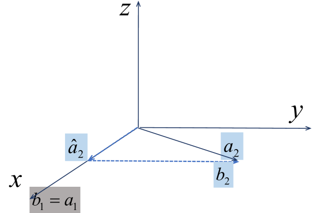
(a) Project $\bm{a}_{2}$ onto the space perpendicular to $\bm{b}_{1}$.

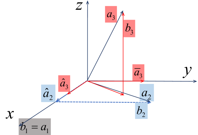
(b) Project $\bm{a}_{3}$ onto the space perpendicular to $\bm{b}_{1},\bm{b}_{2}$.

Figure 1.7: The Gram-Schmidt process.

This procedure can be extended beyond three vectors to an arbitrary set and is known as the Gram-Schmidt process. After applying this process, the matrix $\bm{A}$ is transformed into an upper triangular form. The method is named after Jørgen Pedersen Gram and Erhard Schmidt, though it appeared earlier in the work of Pierre-Simon Laplace within the context of Lie group decomposition theory.

As previously mentioned, the key idea behind QR decomposition is to construct a sequence of orthonormal vectors $\bm{q}_{1},\bm{q}_{2},\ldots$, which successively span the same subspaces as the original vectors:

$$\big{\{}\mathcal{C}([\bm{q}_{1}])=\mathcal{C}([\bm{a}_{1}])\big{\}}\subseteq\big{\{}\mathcal{C}([\bm{q}_{1},\bm{q}_{2}])=\mathcal{C}([\bm{a}_{1},\bm{a}_{2}])\big{\}}\subseteq\big{\{}\mathcal{C}([\bm{q}_{1},\bm{q}_{2},\bm{q}_{3}])=\mathcal{C}([\bm{a}_{1},\bm{a}_{2},\bm{a}_{3}])\big{\}}\subseteq\ldots.$$

This implies that any vector $\bm{a}_{k}$ resides in the space spanned by $\mathcal{C}([\bm{q}_{1},\bm{q}_{2},\ldots,\bm{q}_{k}])$.  Once these orthonormal vectors are determined, the reconstruction of $\bm{a}_{i}$’s from the orthogonal matrix $\bm{Q}=[\bm{q}_{1},\bm{q}_{2},\ldots,\bm{q}_{n}]$ requires an upper triangular matrix $\bm{R}$, such that $\bm{A}=\bm{Q}\bm{R}$.

While the Gram-Schmidt process is a widely used algorithm for QR decomposition, it is not the only approach. Alternative methods, such as Householder reflections and Givens rotations, offer more numerical stability in the presence of round-off errors and may modify the order in which the columns of $\bm{A}$ are processed (lu2021numerical).

1.7.4 Singular Value Decomposition

In eigenvalue decomposition, we factor the matrix into a diagonal matrix. However, this is not always possible. When $\bm{A}$ lacks linearly independent eigenvectors, such diagonalization cannot be achieved. The singular value decomposition (SVD) fills this gap. Instead of using an eigenvector matrix, SVD decomposes a matrix into two orthogonal matrices. Below, we state the theorem for SVD.

Let $\bm{A}\in^{m\times n}$ be any real $m\times n$ matrix with rank $r$. Then, it can be factored as $$\bm{A}=\bm{U}\boldsymbol{\Sigma}\bm{V}^{\top},$$ where $\boldsymbol{\Sigma}\in^{r\times r}$ is a real diagonal matrix, $\boldsymbol{\Sigma}=\mathrm{diag}(\sigma_{1},\sigma_{2}\ldots,\sigma_{r})$ with $\sigma_{1}\geq\sigma_{2}\geq\ldots\geq\sigma_{r}>0$ and The $\sigma_{i}$’s are the nonzero singular values of $\bm{A}$, in the meantime, which are the positive square roots of the nonzero eigenvalues of $\bm{A}^{\top}\bm{A}$ and $\bm{A}\bm{A}^{\top}$. The columns of $\bm{U}\in^{m\times r}$ contain the $r$ eigenvectors of $\bm{A}\bm{A}^{\top}$ corresponding to the $r$ nonzero eigenvalues of $\bm{A}\bm{A}^{\top}$ (semi-orthogonal). The columns of $\bm{V}\in^{n\times r}$ contain the $r$ eigenvectors of $\bm{A}^{\top}\bm{A}$ corresponding to the $r$ nonzero eigenvalues of $\bm{A}^{\top}\bm{A}$ (semi-orthogonal). The columns of $\bm{U}$ and $\bm{V}$ are called the left and right singular vectors of $\bm{A}$, respectively. Furthermore, the columns of both $\bm{U}$ and $\bm{V}$ are mutually orthonormal (by spectral theorem 1.7.2). In particular, the matrix decomposition can be expressed as the sum of outer products of vectors: $$\bm{A}=\bm{U}\boldsymbol{\Sigma}\bm{V}^{\top}=\sum_{i=1}^{r}\sigma_{i}\bm{u}_{i}\bm{v}_{i}^{\top},$$ which is a sum of $r$ rank-one matrices.

By appending $m-r$ additional orthonormal columns to the $r$ eigenvectors of $\bm{A}\bm{A}^{\top}$, we obtain an orthogonal matrix $\bm{U}\in^{m\times m}$. The same process applies to the columns of $\bm{V}$. We then present the full SVD in the following theorem. Differences between the reduced and full SVD are highlighted in blue text. Let $\bm{A}\in^{m\times n}$ be any real $m\times n$ matrix with rank $r$. Then, it can be factored as $$\bm{A}=\bm{U}\boldsymbol{\Sigma}\bm{V}^{\top},$$ where the top-left part of $\boldsymbol{\Sigma}\in$^m×n is a real diagonal matrix, that is $\boldsymbol{\Sigma}=\footnotesize\begin{bmatrix}\boldsymbol{\Sigma}_{1}&\mathbf{0}\\ \mathbf{0}&\mathbf{0}\end{bmatrix}$, where $\boldsymbol{\Sigma}_{1}=\mathrm{diag}(\sigma_{1},\sigma_{2}\ldots,\sigma_{r})\in^{r\times r}$ with $\sigma_{1}\geq\sigma_{2}\geq\ldots\geq\sigma_{r}>0$ and The $\sigma_{i}$’s are the nonzero singular values of matrix $\bm{A}$, which are the positive square roots of the nonzero eigenvalues of $\bm{A}^{\top}\bm{A}$ and $\bm{A}\bm{A}^{\top}$. The columns of $\bm{U}\in{\color[rgb]{0,0.08,0.45}{}^{m\times m}}$ contain the $r$ eigenvectors of $\bm{A}\bm{A}^{\top}$ corresponding to the $r$ nonzero eigenvalues of $\bm{A}\bm{A}^{\top}$ and $m-r$ extra orthonormal vectors from $\mathcal{N}(\bm{A}^{\top})$. The columns of $\bm{V}\in{\color[rgb]{0,0.08,0.45}{}^{n\times n}}$ contain the $r$ eigenvectors of $\bm{A}^{\top}\bm{A}$ corresponding to the $r$ nonzero eigenvalues of $\bm{A}^{\top}\bm{A}$ and $n-r$ extra orthonormal vectors from $\mathcal{N}(\bm{A})$. The columns of $\bm{U}$ and $\bm{V}$ are called the left and right singular vectors of $\bm{A}$, respectively. Furthermore, the columns of $\bm{U}$ and $\bm{V}$ are mutually orthonormal (by spectral theorem 1.7.2), and $\bm{U}$ and $\bm{V}$ are orthogonal matrices. In particular, the matrix decomposition can be expressed as the sum of outer products of vectors: $\bm{A}=\bm{U}\boldsymbol{\Sigma}\bm{V}^{\top}=\sum_{i=1}^{r}\sigma_{i}\bm{u}_{i}\bm{v}_{i}^{\top}$, which is a sum of $r$ rank-one matrices.

In image processing, SVD is also known as the Karhunen-Loewe expansion. The comparison between the reduced and the full SVD is shown in Figure 1.8, where white entries are zero, and blue entries are not necessarily zero.

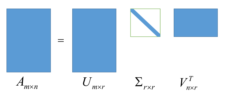
(a) Reduced SVD decomposition.

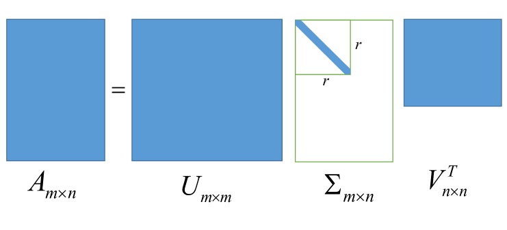
(b) Full SVD decomposition.

Figure 1.8: Comparison between the reduced and full SVD.

1.8 Classes of Rate of Convergence

Before we delve into specific algorithms for solving optimization problems, it is essential to establish criteria for evaluating the speed at which these algorithms converge, as most of them are iterative methods. We define the convergence of a sequence as follows. Note that the $t$-th element in a sequence is denoted by a superscript in parentheses. For instance, $\bm{A}^{(t)}$ denotes the $t$-th matrix in a sequence, and $\bm{a}^{(t)}$ represents the $t$-th vector in a sequence.

Definition 1.91 (Convergence of a Sequence)

Let $\mu^{(1)},\mu^{(2)},\ldots\in$ be an infinite sequence of scalars. The sequence $\{\mu^{(t)}\}_{t>0}$ is said to converge to $\mu^{*}$ if

$$\mathop{\lim}_{t\rightarrow\infty}\left\lvert\mu^{(t)}-\mu^{*}\right\rvert=0.$$

Similarly, let $\boldsymbol{\mu}^{(1)},\boldsymbol{\mu}^{(2)},\ldots\in^{n}$ be an infinite sequence of vectors. The sequence $\{\boldsymbol{\mu}^{(t)}\}_{t>0}$ is said to converge to $\boldsymbol{\mu}^{\star}$ if

$$\mathop{\lim}_{t\rightarrow\infty}\left\lVert\boldsymbol{\mu}^{(t)}-\boldsymbol{\mu}^{\star}\right\rVert=0.$$

The convergence of a sequence of vectors or matrices depends on the norm used. It’s important to note that, according to the equivalence of vector or matrix norms (Theorem 1), if a sequence of vectors or matrices converges in one norm, it will also converge in all other norms.

Definition 1.92 (Linear Convergence)

A sequence $\{\mu^{(t)}\}_{t>0}$ with limit $\mu^{*}$ is said to converge linearly if there exists a constant $c\in(0,1)$ such that

$$\left\lvert\mu^{(t+1)}-\mu^{*}\right\rvert\leq c\left\lvert\mu^{(t)}-\mu^{*}\right\rvert.$$

In other words, the linearly convergent sequence has the following property:

$$\mathop{\lim}_{t\rightarrow\infty}\frac{\left\lvert\mu^{(t+1)}-\mu^{*}\right\rvert}{\left\lvert\mu^{(t)}-\mu^{*}\right\rvert}=c\in(0,1).$$

For example, the sequence $\mu^{(t)}=4+(1/4)^{t}$ converges linearly to $\mu^{*}=4$ since

$$\mathop{\lim}_{t\rightarrow\infty}\frac{\left\lvert\mu^{(t+1)}-\mu^{*}\right\rvert}{\left\lvert\mu^{(t)}-\mu^{*}\right\rvert}=\frac{1}{4}\in(0,1).$$

Definition 1.93 (Superlinear Convergence)

A sequence $\{\mu^{(t)}\}_{t>0}$ with limit $\mu^{*}$ is said to converge superlinearly if there exists a constant $c_{t}>0$ with $c_{t}\rightarrow 0$ such that

$$\left\lvert\mu^{(t+1)}-\mu^{*}\right\rvert\leq c_{t}\left\lvert\mu^{(t)}-\mu^{*}\right\rvert.$$

In other words, the superlinearly convergent sequence has the following property:

$$\mathop{\lim}_{t\rightarrow\infty}\frac{\left\lvert\mu^{(t+1)}-\mu^{*}\right\rvert}{\left\lvert\mu^{(t)}-\mu^{*}\right\rvert}=0.$$

For example, the sequence $\mu^{(t)}=4+\left(\frac{1}{t+4}\right)^{t+3}$ converges superlinearly to $\mu^{*}=4$ since

$$\mathop{\lim}_{t\rightarrow\infty}\frac{\left\lvert\mu^{(t+1)}-\mu^{*}\right\rvert}{\left\lvert\mu^{(t)}-\mu^{*}\right\rvert}=\left(\frac{k+4}{k+5}\right)^{k+3}\frac{1}{k+5}=0.$$

Definition 1.94 (Quadratic Convergence)

A sequence $\{\mu^{(t)}\}_{t>0}$ with limit $\mu^{*}$ is said to converge quadratically if there exists a constant $c>0$ such that

$$\left\lvert\mu^{(t+1)}-\mu^{*}\right\rvert\leq c\left\lvert\mu^{(t)}-\mu^{*}\right\rvert^{2}.$$

In other words, the quadratically convergent sequence has the following property:

$$\mathop{\lim}_{t\rightarrow\infty}\frac{\left\lvert\mu^{(t+1)}-\mu^{*}\right\rvert}{\left\lvert\mu^{(t)}-\mu^{*}\right\rvert^{2}}=c.$$

For example, the sequence $\mu^{(t)}=4+(1/4)^{2^{t}}$ converges quaeratically to $\mu^{*}=4$ since

$$\mathop{\lim}_{t\rightarrow\infty}\frac{\left\lvert\mu^{(t+1)}-\mu^{*}\right\rvert}{\left\lvert\mu^{(t)}-\mu^{*}\right\rvert^{2}}=1.$$

Definition 1.95 (Cubic Convergence)

A sequence $\{\mu^{(t)}\}_{t>0}$ with limit $\mu^{*}$ is said to converge cubically if there exists a constant $c>0$ such that

$$\left\lvert\mu^{(t+1)}-\mu^{*}\right\rvert\leq c\left\lvert\mu^{(t)}-\mu^{*}\right\rvert^{3}.$$

In other words, the cubically convergent sequence has the following property:

$$\mathop{\lim}_{t\rightarrow\infty}\frac{\left\lvert\mu^{(t+1)}-\mu^{*}\right\rvert}{\left\lvert\mu^{(t)}-\mu^{*}\right\rvert^{3}}=c.$$

For example, the sequence $\mu^{(t)}=4+(1/4)^{3^{t}}$ converges cubically to $\mu^{*}=4$ since

$$\mathop{\lim}_{t\rightarrow\infty}\frac{\left\lvert\mu^{(t+1)}-\mu^{*}\right\rvert}{\left\lvert\mu^{(t)}-\mu^{*}\right\rvert^{3}}=1.$$

Chapter 1  Problems 

1. Prove that the sum or maximum of two norms is also a norm.

2. Prove that the $\ell_{1}$ and $\ell_{\infty}$ norms cannot be derived from an inner product. Hint: Consider the standard basis vectors $\bm{e}_{1}$ and $\bm{e}_{2}$, and examine the parallelogram identity in (1.6) or the polarization identity in (1.7).

3. $k$-Norm. Show that the $k$-norm $\left\lVert\bm{x}\right\rVert^{[k]}$ on $\bm{x}\in^{m}$, defined as the sum of the largest $k$ absolute elements of a vector, is a valid norm. Specifically, verify that $\left\lVert\bm{x}\right\rVert_{\infty}=\left\lVert\bm{x}\right\rVert^{[1]}$ and $\left\lVert\bm{x}\right\rVert^{[n]}=\left\lVert\bm{x}\right\rVert_{1}$. Additionally, prove the following sequence of inequalities:

   $$\left\lVert\bm{x}\right\rVert_{\infty}=\left\lVert\bm{x}\right\rVert^{[1]}\leq\left\lVert\bm{x}\right\rVert^{[2]}\leq\ldots\leq\left\lVert\bm{x}\right\rVert^{[n]}=\left\lVert\bm{x}\right\rVert_{1}.$$ (1.36)

4. Given the Cholesky decomposition of a PD matrix: $\bm{A}=\bm{L}\bm{D}\bm{L}^{\top}$, show that $\text{cond}(\bm{A})\geq\text{cond}(\bm{D})$.

5. In Proposition 1.4.1, we demonstrated that eigenvectors corresponding to distinct eigenvalues of a symmetric matrix are orthogonal. More generally, prove that the eigenvectors corresponding to distinct eigenvalues of any matrix are linearly independent.

6. Show that if $\bm{A}$ is positive semidefinite and nonsingular, then $\bm{A}^{-1}$ is positive definite.

7. Quadratic form. Consider the quadratic form $L(\bm{x})=\frac{1}{2}\bm{x}^{\top}\bm{A}\bm{x}-\bm{b}^{\top}\bm{x}+c$ in Equation (1.21), where $\bm{A}\in^{n\times n}$, $\bm{x}\in^{n}$, and $c\in$. Suppose $\bm{A}$ is positive semidefinite. Show that $L(\bm{x})$ is bounded below over ⁿ if and only if $\bm{b}$ is in the column space of $\bm{A}$.

8. Quadratic form. Consider again the quadratic form $L(\bm{x})=\frac{1}{2}\bm{x}^{\top}\bm{A}\bm{x}-\bm{b}^{\top}\bm{x}+c$ in Equation (1.21). Show that $L(\bm{x})$ is coercive  if and only if $\bm{A}$ is PD.

9. Square of symmetric matrices. Let $\bm{A}\in^{n\times n}$ be symmetric. Show that the eigenvalues of $\bm{A}^{2}$ (can only be nonnegative) are the squares of the eigenvalues of $\bm{A}\in^{n\times n}$. What is the relationship between the eigenvectors?

10. Consider the partition of an orthogonal matrix $\bm{Q}=\scriptsize\begin{bmatrix}\underset{p\times p}{\bm{A}}&\underset{p\times q}{\bm{B}}\\ \underset{q\times p}{\bm{C}}&\underset{q\times q}{\bm{D}}\end{bmatrix}\in^{n\times n}.$ Show that $\mathrm{rank}(\bm{B})=\mathrm{rank}(\bm{C})$ and $\mathrm{rank}(\bm{D})=n+\mathrm{rank}(\bm{A})-2p$.

Chapter 2 Optimization and Optimality Conditions

2.1 Classes of Sets and Functions

We briefly introduce different notions of sets and functions.

2.1.1 Interior Points and Closed Sets

Given a specific norm definition, we introduce the concepts of an open ball and a closed ball as follows:

Definition 2.1 (Open Ball, Closed Ball)

Let $\left\lVert\cdot\right\rVert_{p}:^{n}\rightarrow_{+}$ be the $\ell_{p}$ norm function. The open ball centered at $\bm{c}\in^{n}$ with radius $r$ is defined as

$${\mathbb{B}}_{p}(\bm{c},r)\triangleq\{\bm{x}\in^{n}\mid\left\lVert\bm{x}-\bm{c}\right\rVert_{p}<r\}.$$

Similarly, the closed ball centered at $\bm{c}\in^{n}$ with radius $r$ is defined as

$${\mathbb{B}}_{p}[\bm{c},r]\triangleq\{\bm{x}\in^{n}\mid\left\lVert\bm{x}-\bm{c}\right\rVert_{p}\leq r\}.$$

For example, ${\mathbb{B}}_{2}[\mathbf{0},1]$ represents the unit closed ball w.r.t. to the $\ell_{2}$ norm. To simplify notation, we omit the subscript 2 for $\ell_{2}$ norms and $\mathbf{0}$ for balls centered at zero, e.g., ${\mathbb{B}}[1]\triangleq{\mathbb{B}}_{2}[\mathbf{0},1]$. As a special case, the notation ${\mathbb{B}}_{0}[k]\triangleq{\mathbb{B}}_{0}[\mathbf{0},k]$ denotes the set of $k$-sparse vectors, i.e., containing vectors that have only $k$ (or less) nonzero elements. More generally, let $\left\lVert\cdot\right\rVert$ be any norm, the induced open and closed balls are denoted as

$${\mathbb{B}}_{\left\lVert\cdot\right\rVert}(\bm{c},r)\qquad\text{and}\qquad{\mathbb{B}}_{\left\lVert\cdot\right\rVert}[\bm{c},r].$$

Subsequently, we define the concepts of interior and relative interior points. These concepts are foundational in topology and convex analysis and are based on the definitions of balls.

Definition 2.2 (Interior and Relative Interior Points)

The interior of a set ${\mathbb{S}}$ in a topological space is the set of all points in ${\mathbb{S}}$ that have a neighborhood completely contained within ${\mathbb{S}}$. Formally, the interior of ${\mathbb{S}}$, denoted by $\text{int}({\mathbb{S}})$, is given by:

$$\text{int}({\mathbb{S}})=\{\bm{x}\in{\mathbb{S}}\mid\exists\epsilon>0\text{ such that }{\mathbb{B}}(\bm{x},\epsilon)\subseteq{\mathbb{S}}\}.$$

where ${\mathbb{B}}(\bm{x},\epsilon)$ is an open ball centered at $\bm{x}$ with radius $\epsilon$.

The relative interior of a set ${\mathbb{S}}$ in a topological space, typically within the context of convex analysis, is the interior of ${\mathbb{S}}$ relative to its affine hull. The affine hull of ${\mathbb{S}}$, denoted by $\text{aff}({\mathbb{S}})$, is the smallest affine space containing ${\mathbb{S}}$ (Definition 2.18). The relative interior of ${\mathbb{S}}$, denoted by $\text{relint}({\mathbb{S}})$, is given by:

$$\text{relint}({\mathbb{S}})=\{\bm{x}\in{\mathbb{S}}\mid\exists\epsilon>0\text{ such that }{\mathbb{B}}_{\text{aff}({\mathbb{S}})}(\bm{x},\epsilon)\subseteq{\mathbb{S}}\}.$$

where ${\mathbb{B}}_{\text{aff}({\mathbb{S}})}(\bm{x},\epsilon)$ is the open ball centered at $\bm{x}$ with radius $\epsilon$ in the subspace topology of $\text{aff}({\mathbb{S}})$.

In other words, the interior of a set is concerned with the open balls in the ambient space; the relative interior is concerned with open balls in the affine hull of the set, which is particularly important in higher dimensions and in convex analysis where the set may lie in a lower-dimensional subspace.

Example 2.3 (Interior and Relative Interior Points)

Interval in . Let ${\mathbb{S}}=[0,1]$. Then $\text{int}({\mathbb{S}})=(0,1)$ and $\text{relint}({\mathbb{S}})=(0,1)$. Here, the interior and relative interior are the same because the set $[0,1]$ is a subset of and $\text{aff}({\mathbb{S}})=$.

Line Segment in ².

Let ${\mathbb{S}}=\{(x,y)\in^{2}\mid 0\leq x\leq 1,y=0\}$ with $\text{aff}({\mathbb{S}})=\{(x,0)\in^{2}\mid x\in\}$. Then $\text{int}({\mathbb{S}})=\varnothing$ and $\text{relint}({\mathbb{S}})=\{(x,0)\mid 0<x<1\}$. The interior is empty because there are no open balls in ² entirely contained within ${\mathbb{S}}$. However, the relative interior is the open interval (0, 1) in the context of the line segment (the affine hull is the line $y=0$).

Triangle in ².

Let ${\mathbb{S}}$ be a triangle with vertices at $(0,0)$, $(1,0)$, and $(0,1)$. Then the interior consists of all points inside the triangle, excluding the boundary; while the relative interior is the same as the interior in this case because the affine hull of the triangle is the entire plane ². $\square$

Definition 2.4 (Open, Closed, Compact, and Level Sets)

A set ${\mathbb{S}}_{1}$ is said to be open if it consists of only interior points. That is, for every $\bm{x}\in{\mathbb{S}}$, there exists a scalar $s>0$ such that ${\mathbb{B}}(\bm{x},s)\subseteq{\mathbb{S}}_{1}$.

A set ${\mathbb{S}}_{2}$ is said to be closed if its complement $\cancel{{\mathbb{S}}_{2}}$ is open. Alternatively, ${\mathbb{S}}_{2}$ is closed if it contains all the limit points of convergent sequence of points in ${\mathbb{S}}_{2}$; that is, for every sequence of points $\{\bm{x}_{i}\}_{i\geq 1}\subseteq{\mathbb{S}}_{2}$ satisfying $\bm{x}_{i}\rightarrow\bm{x}^{\star}$ as $i\rightarrow\infty$, it follows that $\bm{x}^{\star}\in{\mathbb{S}}_{2}$. In the meantime, the closure of a set ${\mathbb{S}}$, denoted by $\text{cl}({\mathbb{S}})$, is defined as the smallest closed set containing ${\mathbb{S}}$:

$$\text{cl}({\mathbb{S}})=\cap\left\{{\mathbb{T}}\mid{\mathbb{S}}\subseteq{\mathbb{T}},{\mathbb{T}}\text{ is closed}\right\}.$$

A set ${\mathbb{S}}\subseteq^{n}$ is called bounded if there exists $M>0$ for which ${\mathbb{S}}\subseteq{\mathbb{B}}(\mathbf{0},M)$, where ${\mathbb{B}}(\mathbf{0},M)$ is the ball of finite radius $M$ centered at the origin. A set ${\mathbb{S}}\subseteq^{n}$ is called compact if it is closed and bounded.

Given a function $f:{\mathbb{S}}\rightarrow$ where ${\mathbb{S}}\subseteq^{n}$, the level set of $f$ at a particular value $c\in$ is defined as:

$$\mathrm{Lev}[f,c]=\{\bm{x}\in{\mathbb{S}}\mid f(\bm{x})\leq c\}.\leavevmode\nobreak\$$

In other words, the level set $\mathrm{Lev}[f,c]$ consists of all points $\bm{x}$ in the domain ${\mathbb{S}}$ for which the function $f$ evaluates to smaller than or equal to the constant $c$.

2.1.2 Continuous Functions

A continuous function is one that does not exhibit abrupt changes in value—referred to as discontinuities. More formally, it means that small changes in the input of the function lead to correspondingly small changes in its output. Continuous functions are foundational in calculus and analysis, boasting several important properties.

Definition 2.5 (Continuous Functions)

Let $f:{\mathbb{S}}\subseteq^{n}\rightarrow$. The function $f$ is said to be continuous at a point $\bm{y}\in{\mathbb{S}}$ if for every $\epsilon>0$, there exists a $\delta>0$ such that for all $\bm{x}$ in ${\mathbb{S}}$:

$$\forall\,\epsilon>0,\exists\delta>0:\quad\forall\,\bm{x}\in{\mathbb{S}},\left\lVert\bm{x}-\bm{y}\right\rVert_{2}<\delta\quad\implies\quad\left\lvert f(\bm{x})-f(\bm{y})\right\rvert<\epsilon.$$ (2.1)

In simpler terms, this definition indicates that we can make the values of $f(\bm{x})$ arbitrarily close to $f(\bm{y})$ by selecting $\bm{x}$ sufficiently close to $\bm{y}$.

If $f$ is continuous at every point in its domain ${\mathbb{S}}$, then $f$ is said to be continuous on ${\mathbb{S}}$ or simply continuous.

Remark 2.6 (Properties of Continuous Functions)

For a continuous function, we have the following properties:

1. Intermediate value theorem. If $f$ is continuous on a closed interval $[a,b]$ and $y$ is any number between $f(a)$ and $f(b)$, then there exists a $c\in[a,b]$ such that $f(c)=y$.

2. Extreme value theorem. If $f$ is continuous on a closed interval $[a,b]$, then $f$ attains both a maximum and minimum value on that interval (Theorem LABEL:theorem:weierstrass_them).

3. Composition of continuous functions. If $g$ is continuous at $c$ and $f$ is continuous at $g(c)$, then the composition $f\circ g$ is continuous at $c$.

4. Arithmetic operations. If $f$ and $g$ are continuous at $c$, then so are $f+g$, $f-g$, $fg$, and $\frac{f}{g}$ (provided $g(c)\neq 0$).

5. Continuity and limits. A function $f$ is continuous at $c$ if and only if $\lim_{x\to c}f(x)=f(c)$.

Example 2.7 (Continuous Functions)

Following are some continuous functions:

• Polynomial functions are continuous everywhere.

• Rational functions are continuous wherever they are defined (i.e., where the denominator is not zero).

• Trigonometric functions like sine and cosine are continuous everywhere.

• Exponential and logarithmic functions are continuous on their domains.

• Absolute value function $\left\lvert x\right\rvert$ is continuous everywhere.

There are different types of discontinuities:

• Removable discontinuity. The function has a hole at a point, but it can be “filled” to become continuous.

• Jump discontinuity. The left-hand limit and right-hand limit exist but are not equal.

• Infinite discontinuity. The function approaches positive or negative infinity at a point.

• Oscillating discontinuity. The function does not approach a single value as the input approaches a point.

Continuous functions are easier to analyze and manipulate, while discontinuities can lead to complex behaviors that require special handling. Recognizing the type of discontinuity helps in determining appropriate strategies for dealing with these functions in various applications. $\square$

Definition 2.8 (Uniform Continuity)

A function $f:{\mathbb{S}}\subseteq^{n}\rightarrow$ is said to be uniformly continuous on a set ${\mathbb{S}}$ if for every $\epsilon>0$, there exists a $\delta>0$ such that for all $\bm{x}$ and $\bm{y}$ in ${\mathbb{S}}$, whenever the distance between $\bm{x}$ and $\bm{y}$ is less than $\delta$ (that is, $\left\lvert\bm{x}-\bm{y}\right\rvert<\delta$), it follows that the distance between $f(\bm{x})$ and $f(\bm{y})$ is less than $\epsilon$ (that is, $\left\lvert f(\bm{x})-f(\bm{y})\right\rvert<\epsilon$). Formally, $f:{\mathbb{S}}\rightarrow$ is uniformly continuous on ${\mathbb{S}}$ if:

$$\forall\,\epsilon>0,\exists\delta>0:\quad\forall\,\bm{x},{\color[rgb]{0,0.08,0.45}\bm{y}}\in{\mathbb{S}},\left\lVert\bm{x}-\bm{y}\right\rVert_{2}<\delta\quad\implies\quad\left\lvert f(\bm{x})-f(\bm{y})\right\rvert<\epsilon.$$

The key difference between uniform continuity and ordinary (pointwise) continuity is the choice of $\delta$. For pointwise continuity, $\delta$ can depend on both $\epsilon$ and the point $\bm{y}$ in the domain. However, for uniform continuity, $\delta$ must work for all points in the set ${\mathbb{S}}$ simultaneously, given an $\epsilon$.

Uniform continuity is a stronger form of continuity. Every uniformly continuous function is continuous, but not every continuous function is uniformly continuous. Uniform continuity is especially important in analysis because it guarantees certain desirable properties, like the preservation of Cauchy sequences and the ability to interchange limits and function evaluations under suitable conditions.

Example 2.9 (Continuity vs Uniform Continuity)

Consider $f(x)=x^{2}$. For any given $y\in$, we can always find a $\delta$ depending on $y$ and $\epsilon$ to satisfy the definition of continuity. Hence, $f(x)=x^{2}$ is continuous at every point $y\in$.

Not uniformly continuous.

To show that $f(x)=x^{2}$ is not uniformly continuous on , consider two sequences $x_{t}=t$ and $y_{t}=t+\frac{1}{t}$ where $t$ is an integer. As $t\to\infty$, the distance between $x_{t}$ and $y_{t}$ approaches 0 ($\left\lvert x_{t}-y_{t}\right\rvert=\frac{1}{t}\to 0$), but the difference in function values does not approach 0:

$$\left\lvert f(x_{t})-f(y_{t})\right\rvert=\left\lvert t^{2}-\left(t+\frac{1}{t}\right)^{2}\right\rvert=\left\lvert t^{2}-\left(t^{2}+2+\frac{1}{t^{2}}\right)\right\rvert=\left\lvert-2-\frac{1}{t^{2}}\right\rvert\to 2$$

Since the difference in function values does not become arbitrarily small even when the inputs are arbitrarily close, $f(x)=x^{2}$ is not uniformly continuous on . This shows that while $f(x)=x^{2}$ is continuous everywhere on the real line, it fails to be uniformly continuous because the required $\delta$ in the definition of uniform continuity cannot be chosen independently of $x$. $\square$

Remark 2.10 (Consequence of Uniform Continuity)

Let $\nabla f$ be uniformly continuous. Then,

$$\left\langle\nabla f(\bm{x}_{1}),\bm{d}\right\rangle=\left\langle\nabla f(\bm{x}_{2}),\bm{d}\right\rangle+o(\left\lVert\bm{d}\right\rVert_{2}),\quad\text{where }\bm{d}\triangleq\bm{x}_{1}-\bm{x}_{2}.$$

To see this, by the definition of uniform continuity, for any $\epsilon>0$, there exists a $\delta>0$ such that:

$$\left\lVert\bm{d}\right\rVert_{2}<\delta\quad\implies\quad\left\lVert\nabla f(\bm{x}_{1})-\nabla f(\bm{x}_{2})\right\rVert_{2}<\epsilon.$$

This implies that as $\left\lVert\bm{d}\right\rVert_{2}\to 0$, we can choose $\delta$ arbitrarily small, and the gradient difference satisfies: $\left\lVert\nabla f(\bm{x}_{1})-\nabla f(\bm{x}_{2})\right\rVert_{2}=o(1).$ Using the linearity of the inner product, we can write:

$$\left\langle\nabla f(\bm{x}_{1}),\bm{d}\right\rangle=\left\langle\nabla f(\bm{x}_{2}),\bm{d}\right\rangle+\left\langle\nabla f(\bm{x}_{1})-\nabla f(\bm{x}_{2}),\bm{d}\right\rangle,$$

where $\left\langle\nabla f(\bm{x}_{1})-\nabla f(\bm{x}_{2}),\bm{d}\right\rangle=\left\lVert\nabla f(\bm{x}_{1})-\nabla f(\bm{x}_{2})\right\rVert_{2}\cdot\left\lVert\bm{d}\right\rVert_{2}\cdot\cos(\theta),$ and $\theta$ is the angle between $\nabla f(\bm{x}_{1})-\nabla f(\bm{x}_{2})$ and $\bm{d}$. Since $\left\lVert\nabla f(\bm{x}_{1})-\nabla f(\bm{x}_{2})\right\rVert_{2}=o(1)$, we have: $\left\langle\nabla f(\bm{x}_{1})-\nabla f(\bm{x}_{2}),\bm{d}\right\rangle=o(\left\lVert\bm{d}\right\rVert_{2}).$ Therefore, combining these results, we get the desired result.

Definition 2.11 (Lower Semicontinuity)

A function $f:^{n}\rightarrow\cup\{-\infty,\infty\}$ is called lower semicontinuous at $\bm{x}^{*}\in^{n}$ if

$$f(\bm{x})\leq\liminf_{t\rightarrow\infty}f(\bm{x}^{(t)})$$

for any sequence $\{\bm{x}^{(t)}\}_{t\geq 1}\subseteq^{n}$ for which $\bm{x}^{(t)}\rightarrow\bm{x}^{*}$ as $t\rightarrow\infty$. In other words, the limit inferior of the function values at points approaching $\bm{x}^{*}$ must be greater than or equal to the function value at $\bm{x}^{*}$ . This means that the function does not have any sudden drops as you approach $\bm{x}^{*}$. A function $f:^{n}\rightarrow\cup\{-\infty,\infty\}$ is called lower semicontinuous if it is lower semicontinuous at each point in ⁿ.

Note that including $\{-\infty,\infty\}$ in the codomain of a function when defining lower semicontinuityis not strictly necessary for all functions, but it allows for greater generality and flexibility in mathematical analysis. Some functions may have points where they tend towards infinity, either positively or negatively. By including $\{-\infty,\infty\}$, we can still discuss the continuity properties of such functions at those points.

Figure 2.1 depicts examples of lower semicontinuous and non-lower semicontinuous functions. In optimization problems, lower semicontinuity plays a key role because it guarantees that if a sequence of feasible points approaches a minimum, then the limit of this sequence will also be a feasible point and will achieve the minimum value. This property ensures that optimal solutions exist under certain conditions. In many applications, especially in calculus of variations and optimal control, lower semicontinuity is used to prove the existence of minimizers of functionals. If a functional is lower semicontinuous and coercive (it tends to infinity as the norm of its argument grows), then under some compactness assumptions, one can show that there exists a minimizer; see LABEL:weier2_prop_close in Theorem LABEL:theorem:weierstrass_them. In numerical methods and iterative algorithms, lower semicontinuity can help in proving convergence properties. For instance, if a sequence generated by an algorithm is minimizing a lower semicontinuous function, it can be shown that the limit points of the sequence are stationary points; for example, the lower semicontinuity can be applied to prove the uniqueness of the optimizer for a closed and strongly convex function (Theorem LABEL:theorem:exi_close_sc). For this reason, in most of our discussions, we consider lower semicontinuous (closed) functions for evaluation.

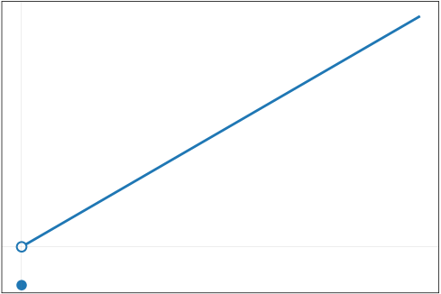
(a) A lower semicontinuous funtion.

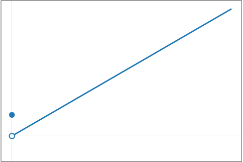
(b) A non-lower semicontinuous funtion

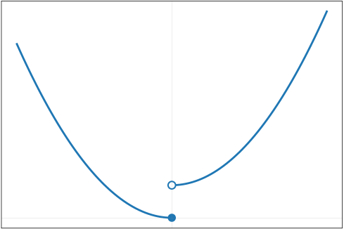
(c) A lower semicontinuous funtion.

Figure 2.1: Lower semicontinuous and non-lower semicontinous funtions. In numerical methods and iterative algorithms, lower semicontinuity can help in proving convergence properties. For instance, if a sequence generated by an algorithm is minimizing a lower semicontinuous function, it can be shown that the limit points of the sequence are stationary points.

2.1.3 Extended Real-Valued Functions

Extended real-valued functions are those that can take values from the extended real number line, which includes all real numbers along with two additional elements: positive infinity ($+\infty$) and negative infinity ($-\infty$). These functions are widely used in mathematical analysis, optimization theory, and measure theory, providing a convenient framework to handle limits and boundary conditions.

Definition 2.12 (Extended Real-Valued, Proper, Closed Functions)

An extended real-valued function $f$ is a function defined on a set ${\mathbb{S}}$ (often a subset of ⁿ or another topological space) that maps each point $\bm{x}$ in ${\mathbb{S}}$ to a value in the extended real number line $\widehat{\mathbb{R}}=\cup\{-\infty,\infty\}$. Formally, an extended real-valued function is written as:

$$f:{\mathbb{S}}\rightarrow\widehat{\mathbb{R}}\qquad\text{or}\qquad f:{\mathbb{S}}\rightarrow\cup\{-\infty,\infty\}.$$

The effective domain or simply the domain and the epigraph of an extended real-valued function are the sets:

$$\textbf{(domain)}: \mathrm{dom}(f) \triangleq \{\bm{x}\in{\mathbb{S}}:f(\bm{x})<\infty\};$$

$$\textbf{(epigraph)}: \mathrm{epi}(f) \triangleq \{(\bm{x},r)\in{\mathbb{S}}\times:f(\bm{x})\leq r\}.$$

That is, the epigraph of an extended real-valued function $f$ is the set of points lying on or above its graph.

In the meantime, a function $f:{\mathbb{S}}\rightarrow\widehat{\mathbb{R}}$ is called proper if it satisfies the following two conditions:

1. Non-identically infinite. The function does not attain the value $+\infty$ everywhere in its domain. In other words, there exists at least one point $\bm{x}\in{\mathbb{S}}$ such that $f(\bm{x})<+\infty$.

2. No negative infinity values. The function never takes on the value $-\infty$. That is, for all $\bm{x}\in{\mathbb{S}},f(\bm{x})>-\infty$.

These conditions ensure that the function has some finite values and avoids the undefined behavior associated with $-\infty$. For a proper function, this domain is nonempty because of the first condition above.

A function $f$ is said to be closed if its epigraph is a closed set in the product topology of ${\mathbb{S}}\times$. In other words, for every sequence $(\bm{x}^{(t)},r_{t})$ in $\text{epi}(f)$ that converges to a limit $(\bm{x}^{*},r^{*})$, we have $f(\bm{x}^{*})\leq r^{*}$, meaning that the limit point $(\bm{x}^{*},r^{*})$ also belongs to the epigraph.

Definition 2.13 (Coerciveness)

Let $f:^{n}\rightarrow$ be a continuous function defined over ⁿ. The function $f$ is called coercive if

$$\lim_{\left\lVert\bm{x}\right\rVert_{2}\rightarrow\infty}f(\bm{x})=\infty.$$

Exercise 2.14 (Coerciveness of Quadratic Functions)

Let $f(\bm{x})=\frac{1}{2}\bm{x}^{\top}\bm{A}\bm{x}+\bm{b}^{\top}\bm{x}+c$, where $\bm{A}\in^{n\times n}$ is symmetric, $\bm{b}\in^{n}$, and $c\in$. Show that $f(\bm{x})$ is coercive if $\bm{A}$ is positive definite.

Proper functions are particularly significant in convex analysis and optimization theory because they allow for a well-defined notion of minimization. When dealing with optimization problems, one often seeks to minimize a function over a given set. A proper function ensures that there are feasible points to consider (points where the function value is finite), which is necessary for the problem to be meaningful. Therefore, unless otherwise stated, we only consider proper functions in this book. Moreover, many results in convex analysis require the objective function to be proper. For example, the Fenchel-Moreau theorem, which relates a function to its biconjugate, requires the function to be proper, convex, and lower semi-continuous.

Example 2.15 (Proper Functions)

The following functions are proper:

• A linear function $f(x)=ax+b$ on is proper since it never reaches $\pm\infty$.

• The indicator function $\delta_{\mathbb{S}}(\bm{x})$, which is $0$ if $\bm{x}$ belongs to a set ${\mathbb{S}}$ and $+\infty$ otherwise, is proper if ${\mathbb{S}}$ is nonempty.

• The function $f(x)=\frac{1}{x}$ on is not proper since it tends to $+\infty$ as $x$ approaches $0$ from the positive side and to $-\infty$ from the negative side.

Consider why the non-proper function $f(x)=\frac{1}{x}$ is not well-defined for a minimization problem. $\square$

Exercise 2.16 (Closedness of Indicator)

Show that the indicator function $\delta_{\mathbb{S}}$, which is $0$ if $\bm{x}$ belongs to a set ${\mathbb{S}}$ and $+\infty$ otherwise, is closed if and only if ${\mathbb{S}}$ is a closed set.

Let $f:^{n}\rightarrow\cup\{-\infty,\infty\}$. Then the following three statements are equivalent: (i) $f$ is lower semicontinuous. (ii) $f$ is closed. (iii) For any $\alpha\in$, the level set $\mathrm{Lev}[f,\alpha]=\{\bm{x}\in^{n}\mid f(\bm{x})\leq\alpha\}$ is closed.

Proof [of Theorem 2.1.3] (i) $\implies$ (ii). Assume that $f$ is lower semicontinuous. We will demonstrate that $\mathrm{epi}(f)$ is closed. Let $\{(\bm{x}^{(t)},y^{(t)})\}_{t\geq 1}\subseteq\mathrm{epi}(f)$ be a sequence such that $(\bm{x}^{(t)},y^{(t)})\rightarrow(\bm{x}^{*},y^{*})$ as $t\rightarrow\infty$. By definition, for any $t\geq 1$,

$$f(\bm{x}^{(t)})\leq y^{(t)}.$$

Due to the lower semicontinuity of $f$ at $\bm{x}^{*}$, we have

$$f(\bm{x}^{*})\leq\liminf_{t\rightarrow\infty}f(\bm{x}^{(t)})\leq\liminf_{t\rightarrow\infty}y^{(t)}=y^{*},$$

which shows that $(\bm{x}^{*},y^{*})\in\mathrm{epi}(f)$, proving that $f$ is closed.

(ii) $\implies$ (iii).

Suppose that $f$ is closed, i.e., the epigraph $\mathrm{epi}(f)$ is closed. For any $\alpha\in$, we aim to show that $\mathrm{Lev}[f,\alpha]$ is closed. If $\mathrm{Lev}[f,\alpha]=\varnothing$, the claim holds trivially. Otherwise, take a sequence $\{\bm{x}^{(t)}\}_{t\geq 1}\subseteq\mathrm{Lev}[f,\alpha]$ that converges to $\widehat{\bm{x}}$. Obviously, $(\bm{x}^{(t)},\alpha)\in\mathrm{epi}(f)$ for any $t$ and $(\bm{x}^{(t)},\alpha)\rightarrow(\widehat{\bm{x}},\alpha)$ as $t\rightarrow\infty$. By the closedness of $\mathrm{epi}(f)$, it follows that $(\widehat{\bm{x}},\alpha)\in\mathrm{epi}(f)$, establishing the fact that $\widehat{\bm{x}}\in\mathrm{Lev}[f,\alpha]$.

(iii) $\implies$ (i).

Assuming all level sets of $f$ are closed, we prove that it is lower semicontinuous. Suppose for contradiction that $f$ is not lower semicontinuous, meaning that there exists $\bm{x}^{*}\in^{n}$ and $\{\bm{x}^{(t)}\}_{t\geq 1}\subseteq^{n}$ such that $\bm{x}^{(t)}\rightarrow\bm{x}^{*}$ and $\liminf_{t\rightarrow\infty}f(\bm{x}^{(t)})<f(\bm{x}^{*})$. Choose $\alpha$ satisfying

$$\liminf_{t\rightarrow\infty}f(\bm{x}^{(t)})<\alpha<f(\bm{x}^{*}).$$ (2.2)

Then there exists a subsequence $\{\bm{x}_{n_{t}}\}_{t\geq 1}$ such that $f(\bm{x}_{n_{t}})\leq\alpha$ for all $t\geq 1$. By the closedness of the level set $\mathrm{Lev}[f,\alpha]$ and the fact that $\bm{x}_{n_{t}}\rightarrow\bm{x}^{*}$ as $t\rightarrow\infty$, it follows that $f(\bm{x}^{*})\leq\alpha$, which is a contradiction to (2.2), establishing that (iii) implies (i).  

2.1.4 Convex Functions

This subsection introduces the concepts of affine, convex, and conic combinations and hulls within the context of vector sets in ⁿ, providing definitions and mathematical formulations for these fundamental geometric constructs.

Definition 2.18 (Affine/Convex/Conic Combinations and Hulls)

Given a set of vectors $\bm{x}_{1},\bm{x}_{2},\ldots,\bm{x}_{p}\in^{n}$, an affine combination of these $p$ vectors is a vector of the form $\sum_{i=1}^{p}\lambda_{i}\bm{x}_{i}$, where $\sum_{i=1}^{p}\lambda_{i}=1$, i.e., a linear combination of these points where the coefficients (not necessarily nonnegative) sum to 1; a convex combination of these $p$ vectors is a vector of the form $\sum_{i=1}^{p}\lambda_{i}\bm{x}_{i}$, where $\lambda_{i}\geq 0$ for $i\in\{1,2,\ldots,p\}$ satisfying $\sum_{i=1}^{p}\lambda_{i}=1$ (i.e., $\{\lambda_{i}\}$ belongs to the unit-simplex in ^p); when only requiring $\lambda_{i}\geq 0$ without the constraint on their sum, the combination is referred to as a conic combination of these vectors.

The affine hull of a set ${\mathbb{S}}$ is the smallest affine space (a translation of a vector subspace) that contains ${\mathbb{S}}$. Formally, given a set ${\mathbb{S}}\subseteq^{n}$, the affine hull of ${\mathbb{S}}$, denoted as $\text{aff}({\mathbb{S}})$, is defined as the set of all affine combinations of points from ${\mathbb{S}}$:

$$\text{aff}({\mathbb{S}})\triangleq\left\{\sum_{i=1}^{p}\lambda_{i}\bm{x}_{i}\mid\bm{x}_{1},\bm{x}_{2},\ldots,\bm{x}_{p}\in{\mathbb{S}},\lambda_{i}\in,\mathbf{1}^{\top}\boldsymbol{\lambda}=1,p\in\mathbb{N}\right\}.$$

The convex hull of ${\mathbb{S}}$, denoted as $\text{conv}({\mathbb{S}})$, is the set comprising all the convex combinations of vectors from ${\mathbb{S}}$:

$$\text{conv}({\mathbb{S}})\triangleq\left\{\sum_{i=1}^{p}\lambda_{i}\bm{x}_{i}\mid\bm{x}_{1},\bm{x}_{2},\ldots,\bm{x}_{p}\in{\mathbb{S}},\boldsymbol{\lambda}\in\Delta_{p},p\in\mathbb{N}\right\}.$$

Similarly, the conic hull of ${\mathbb{S}}$, denoted as $\text{cone}({\mathbb{S}})$, is the set comprising all the conic combinations of vectors from ${\mathbb{S}}$:

$$\text{cone}({\mathbb{S}})\triangleq\left\{\sum_{i=1}^{p}\lambda_{i}\bm{x}_{i}\mid\bm{x}_{1},\bm{x}_{2},\ldots,\bm{x}_{p}\in{\mathbb{S}},\boldsymbol{\lambda}\in^{n}_{+},p\in\mathbb{N}\right\}.$$

Exercise 2.19 (Closedness of Conic Hull of a Finite Set)

Let $\bm{x}_{1},\bm{x}_{2},\ldots,\bm{x}_{p}\in^{n}$. Show that $\text{cone}(\{\bm{x}_{1},\bm{x}_{2},\ldots,\bm{x}_{p}\})$ is closed.

Exercise 2.20 (Closure)

Show that

$$\text{cl}(_{++}^{n}) =_{+}^{n};$$

$$\text{cl}({\mathbb{B}}(\bm{x},r)) ={\mathbb{B}}[\bm{x},r],\quad\text{where $\bm{x}\in^{n}$, $r\in_{++}$};$$

$$\text{cl}((\bm{x},\bm{y})) =[\bm{x},\bm{y}],\quad\text{where $\bm{x},\bm{y}\in^{n}$ and $\bm{y}\geq\bm{x}$}.$$

Exercise 2.21 (Interior and Closure)

Let ${\mathbb{S}}\subseteq^{n}$ be a convex set with a nonempty interior. Show that

$$\text{cl}(\text{int}({\mathbb{S}}))=\text{cl}({\mathbb{S}})\qquad\text{and}\qquad\text{int}(\text{cl}({\mathbb{S}}))=\text{int}({\mathbb{S}}).$$

For vectors $\bm{x}$ and $\bm{y}$, the point $\lambda\bm{x}+(1-\lambda)\bm{y}$, where $\lambda\in[0,1]$, is known as a convex combination of the two vectors. A set that is closed under arbitrary convex combinations is referred to as a convex set. The standard definition follows:

Definition 2.22 (Convex Set)

A set ${\mathbb{S}}\subseteq^{n}$ is called convex if, for any $\bm{x},\bm{y}\in{\mathbb{S}}$ and $\lambda\in[0,1]$, the point $\lambda\bm{x}+(1-\lambda)\bm{y}$ also belongs to ${\mathbb{S}}$.

Geometrically, convex sets contain all line segments that join two points within the set (Figure 2.2). Consequently, these sets do not feature any concave indentations.

Definition 2.23 (Cone and Convex Cone)

A set ${\mathbb{S}}\subseteq^{n}$ is a cone if for every $\bm{x}\in{\mathbb{S}}$, $\alpha\bm{x}\in{\mathbb{S}}$ for any $\alpha\geq 0$. A set ${\mathbb{S}}$ is a convex cone if it is both a cone and a convex set.

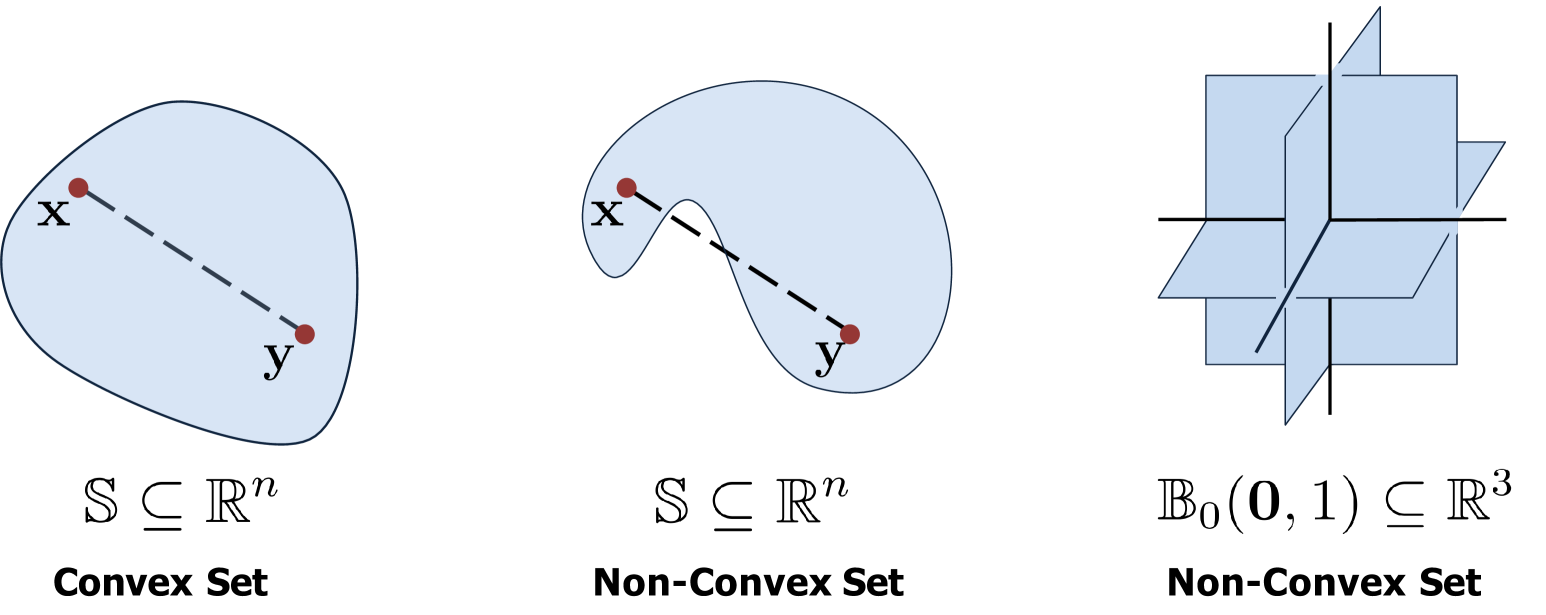
Figure 2.2: A set is considered convex if it includes all convex combinations of its points. If there exists even one convex combination that lies outside the set, then by definition, the set is not convex. Therefore, a convex set must have a shape without any inward “dents” or “bulges”. It’s worth noting that the collection of sparse vectors does not satisfy this criterion and thus forms a non-convex set. The illustration provided is adapted from jain2017non.

A related concept is that of convex functions, which exhibit specific behavior under convex combinations. We now recall the definition:

Definition 2.24 (Convex Functions)

A function $f:{\mathbb{S}}\rightarrow$ defined over a convex set ${\mathbb{S}}\subseteq^{n}$ is called convex if

$$f(\lambda\bm{x}+(1-\lambda)\bm{y})\leq\lambda f(\bm{x})+(1-\lambda)f(\bm{y}),\text{ for any }\bm{x},\bm{y}\in{\mathbb{S}},\lambda\in[0,1].$$

Moreover, $f$ is called strictly convex if

$$f(\lambda\bm{x}+(1-\lambda)\bm{y})<\lambda f(\bm{x})+(1-\lambda)f(\bm{y}),\text{ for any }\bm{x}\neq\bm{y}\in{\mathbb{S}},\lambda\in(0,1).$$

A well-known inequality derived from the concept of convex functions is provided below without a proof. Let $f:{\mathbb{S}}\rightarrow$ be a convex function defined on a convex subset ${\mathbb{S}}\subseteq^{n}$. For any finite sequence of points $\bm{x}_{1},\bm{x}_{2},\ldots,\bm{x}_{m}\in{\mathbb{S}}$ and any sequence of nonnegative weights $\lambda_{1},\lambda_{2},\lambda_{3},\ldots,\lambda_{m}$ such that $\sum_{i=1}^{m}\lambda_{i}=1$, Jensen’s inequality states: $$f\left(\sum_{i=1}^{m}\lambda_{i}\bm{x}_{i}\right)\leq\sum_{i=1}^{m}\lambda_{i}f(\bm{x}_{i}).$$ If $f$ is concave, the inequality is reversed: $$f\left(\sum_{i=1}^{m}\lambda_{i}\bm{x}_{i}\right)\geq\sum_{i=1}^{m}\lambda_{i}f(\bm{x}_{i}).$$ In the context of probability theory, if ${\mathbf{x}}$ is a random vector with values in ${\mathbb{S}}$ and $f$ is a convex function, Jensen’s inequality can be stated as follows: $$f(\mathbb{E}[{\mathbf{x}}])\leq\mathbb{E}[f({\mathbf{x}})],$$ where $\mathbb{E}[\cdot]$ denotes the expectation operator over the random vector ${\mathbf{x}}$. For a concave function, the inequality is again reversed.

Similarly, we provide the definition of quasi-convexity and strict quasi-convexity.

Definition 2.26 (Quasi-Convex Function)

Let $f:{\mathbb{S}}\subseteq^{n}\rightarrow$ be a function defined over the convex set ${\mathbb{S}}$. Then $f$ is called quasi-convex if for any $\mu\in$ the level set $\mathrm{Lev}[f,\mu]$ is convex. Formally, it satisfies that

$$f(\lambda\bm{x}+(1-\lambda)\bm{y})\leq\max\{f(\bm{x}),f(\bm{y})\},\text{ for any }\bm{x},\bm{y}\in{\mathbb{S}},\lambda\in[0,1].$$

Similarlly, $f$ is called strictly quasi-convex if

$$f(\lambda\bm{x}+(1-\lambda)\bm{y})<\max\{f(\bm{x}),f(\bm{y})\},\text{ for any }\bm{x}\neq\bm{y}\in{\mathbb{S}},\lambda\in(0,1).$$

The geometric interpretation of a quasi-convex function is that the value of the function on any line segment within its domain does not exceed the maximum value of the function at the endpoints of the segment. Quasi-convexity is a broader property than convexity since all convex functions are also quasi-convex, but not all quasi-convex functions are convex. For example, $f(x)=\sqrt{\left\lvert x\right\rvert}$ is a quasi-convex function, but it is not convex. Although a quasi-convex function is not necessarily a convex function, its level sets are convex, and it can include some well-behaved non-convex functions (Theorem LABEL:theorem:uni_qua_conv).

In scenarios involving multiple variables, the input vector $\bm{x}$ can be partitioned into $\bm{x}=(\bm{a},\bm{b})\in^{n}$. When discussing properties of functions in this context, convexity can sometimes be referred to as joint convexity, meaning that the function is convex with respect to all components of the input simultaneously. Additionally, there are instances where a function exhibits partial convexity, often termed marginal convexity, indicating that the function is convex when considered with respect to one or more subsets of its input variables while keeping others constant.

Definition 2.27 (Marginally Convex)

A function $f(\bm{a},\bm{b}):{\mathbb{S}}\subseteq^{n}\rightarrow$ (i.e., $(\bm{a},\bm{b})\in^{n}$), defined over a convex set ${\mathbb{S}}$, is called marginally convex if

$$f(\lambda\bm{x}+(1-\lambda)\bm{y},\bm{b})\leq\lambda f(\bm{x},\bm{b})+(1-\lambda)f(\bm{y},\bm{b}),\text{ for any }(\bm{x},\bm{b}),(\bm{y},\bm{b})\in{\mathbb{S}},\lambda\in[0,1].$$

Exercise 2.28

Show that the norm functions $\left\lVert\bm{x}\right\rVert_{2}^{2}$ and $\left\lVert\bm{x}\right\rVert_{1}$ are convex.

Exercise 2.29

Suppose the continuously differentiable function $f$ is convex. Show that the directional derivative (Definition 1.63) $g(\bm{d})\triangleq f^{\prime}(\bm{x};\bm{d})$ is also convex.

Exercise 2.30 (Convexity of Quadratic Functions)

Let $f(\bm{x})=\frac{1}{2}\bm{x}^{\top}\bm{A}\bm{x}+\bm{b}^{\top}\bm{x}+c$, where $\bm{A}\in^{n\times n}$ is symmetric, $\bm{b}\in^{n}$, and $c\in$. Show that $f(\bm{x})$ is convex (resp. strict convex) if and only if $\bm{A}\succeq\mathbf{0}$ (resp. $\bm{A}\succ\mathbf{0}$)

Exercise 2.31 (Closure of Convex)

Let ${\mathbb{S}}\subseteq^{n}$ be a convex set. Show that $\text{cl}({\mathbb{S}})$ is also convex.

Exercise 2.32 (Convexity of Indicator)

Show that the indicator function $\delta_{\mathbb{S}}$, which is $0$ if $\bm{x}$ belongs to a set ${\mathbb{S}}$ and $+\infty$ otherwise, is convex if and only if ${\mathbb{S}}$ is a convex set.

First-order characterizations of convex functions.

Convex functions do not necessarily have to be differentiable. However, when they are differentiable, such functions can be characterized by the gradient inequality. Let $f:{\mathbb{S}}\rightarrow$ be a continuously differentiable function defined on a convex set ${\mathbb{S}}\subseteq^{n}$. Then, $f$ is convex over ${\mathbb{S}}$ if and only if $$f(\bm{x})+\nabla f(\bm{x})^{\top}(\bm{y}-\bm{x})\leq f(\bm{y}),\text{ for any $\bm{x},\bm{y}\in{\mathbb{S}}$}.$$ (2.3) Similarly, the function is strictly convex over ${\mathbb{S}}$ if and only if $$f(\bm{x})+\nabla f(\bm{x})^{\top}(\bm{y}-\bm{x})<f(\bm{y}),\text{ for any $\bm{x}\neq\bm{y}\in{\mathbb{S}}$}.$$ (2.4) This indicates that the graph of a convex function lies above its tangent plane at any point. For concave or strictly concave functions, the inequality signs are reversed.

Proof [of Theorem 2.1.4] For brevity, we only prove (2.3), and (2.4) can be proved analogously. Suppose first that $f$ is convex. Let $\bm{x},\bm{y}\in{\mathbb{S}}$ and $\lambda\in[0,1]$. If $\bm{x}=\bm{y}$, then (2.3) trivially holds. We will therefore assume that $\bm{x}\neq\bm{y}$. Then, the definition of convexity shows that

$$f(\lambda\bm{y}+(1-\lambda)\bm{x})\leq\lambda f(\bm{y})+(1-\lambda)f(\bm{x})\;\implies\;\frac{f(\bm{x}+\lambda(\bm{y}-\bm{x}))-f(\bm{x})}{\lambda}\leq f(\bm{y})-f(\bm{x}).$$

Taking $\lambda\to 0^{+}$, the left-hand side converges to the directional derivative of $f$ at $\bm{x}$ in the direction $\bm{y}-\bm{x}$ (Definition 1.63), whence we have $f^{\prime}(\bm{x};\bm{y}-\bm{x})\leq f(\bm{y})-f(\bm{x}).$ Since $f$ is continuously differentiable, it follows that $f^{\prime}(\bm{x};\bm{y}-\bm{x})=\nabla f(\bm{x})^{\top}(\bm{y}-\bm{x})$ by (1.22), and hence (2.3) follows.

Conversely, assume that the gradient inequality holds. Let $\bm{x},\bm{y}\in{\mathbb{S}}$, and let $\lambda\in[0,1]$. We will show that $f(\lambda\bm{x}+(1-\lambda)\bm{y})\leq\lambda f(\bm{x})+(1-\lambda)f(\bm{y})$. The cases for $\lambda=0$ or $\lambda=1$ holds trivially. We will therefore assume that $\lambda\in(0,1)$. Let $\bm{a}\triangleq\lambda\bm{x}+(1-\lambda)\bm{y}\in{\mathbb{S}}$. Then $-\frac{\lambda}{1-\lambda}(\bm{x}-\bm{a})=(\bm{y}-\bm{a}).$ Combining with the gradient inequality implies that

$$f(\bm{a})+\nabla f(\bm{a})^{\top}(\bm{x}-\bm{a})\leq f(\bm{x})\qquad\text{and}\qquad f(\bm{a})-\frac{\lambda}{1-\lambda}\nabla f(\bm{a})^{\top}(\bm{x}-\bm{a})\leq f(\bm{y}).$$

Multiplying the first inequality by $\frac{\lambda}{1-\lambda}$ and adding it to the second one, we obtain $\frac{1}{1-\lambda}f(\bm{a})\leq\frac{\lambda}{1-\lambda}f(\bm{x})+f(\bm{y}),$ establishing the desired result.  

Let $f:{\mathbb{S}}\rightarrow$ be a continuously differentiable function defined over a convex set ${\mathbb{S}}\subseteq^{n}$. Then, given any $\bm{x},\bm{y}\in{\mathbb{S}}$, $f$ is convex over ${\mathbb{S}}$ if and only if $$\big{(}\nabla f(\bm{x})-\nabla f(\bm{y})\big{)}^{\top}(\bm{x}-\bm{y})\geq 0.$$ (2.5) Similarly, given any $\bm{x}\neq\bm{y}\in{\mathbb{S}}$, $f$ is strictly convex over ${\mathbb{S}}$ if and only if $$\big{(}\nabla f(\bm{x})-\nabla f(\bm{y})\big{)}^{\top}(\bm{x}-\bm{y})>0.$$ (2.6)

Proof [of Theorem 2.1.4] For brevity, we only prove (2.5), and (2.6) can be proved analogously. Assume that $f$ is convex over ${\mathbb{S}}$. Then by the gradient inequality, for any $\bm{x},\bm{y}\in{\mathbb{S}}$, we have

$$f(\bm{x})\geq f(\bm{y})+\nabla f(\bm{y})^{\top}(\bm{x}-\bm{y})\qquad\text{and}\qquad f(\bm{y})\geq f(\bm{x})+\nabla f(\bm{x})^{\top}(\bm{y}-\bm{x}).$$

Summing the two inequalities yields the desired inequality in (2.5).

Conversely, assume that (2.5) holds, and let $\bm{x},\bm{y}\in{\mathbb{S}}$. Define $g(\mu)\triangleq f(\bm{x}+\mu(\bm{y}-\bm{x})),\mu\in[0,1]$ as a one-dimensional function. By the fundamental theorem of calculus (Theorem 1.6), we have

$$f(\bm{y}) =g(1)=g(0)+\int_{0}^{1}g^{\prime}(\mu)\,d\mu=f(\bm{x})+\int_{0}^{1}(\bm{y}-\bm{x})^{\top}\nabla f\big{(}\bm{x}+\mu(\bm{y}-\bm{x})\big{)}\,d\mu$$

$$=f(\bm{x})+\nabla f(\bm{x})^{\top}(\bm{y}-\bm{x})+\int_{0}^{1}(\bm{y}-\bm{x})^{\top}\big{(}\nabla f(\bm{x}+\mu(\bm{y}-\bm{x}))-\nabla f(\bm{x})\big{)}\,d\mu$$

$$\geq f(\bm{x})+\nabla f(\bm{x})^{\top}(\bm{y}-\bm{x}),$$

where the last inequality follows from the monotonicity of the gradient. This shows that $f$ is convex by Definition 2.24.  

Second-order characterizations of convex functions.

When the function is further assumed to be twice continuously differentiable, its convexity can be characterized by the positive semidefiniteness (see Definition 1.57) of the Hessian matrix Let $f:{\mathbb{S}}\subseteq^{n}\rightarrow$ be a twice continuously differentiable function defined on an open convex set ${\mathbb{S}}$, then the function is convex if and only if $\nabla^{2}f(\bm{x})\succeq\mathbf{0}$ for any $\bm{x}\in{\mathbb{S}}$.  Moreover, if $\nabla^{2}f(\bm{x})\succ\mathbf{0}$ for any $\bm{x}\in{\mathbb{S}}$, then the function is strictly convex over ${\mathbb{S}}$ .

Proof [of Theorem 2.1.4] Assume that $\nabla^{2}f(\bm{x})\succeq\mathbf{0}$ for all $\bm{x}\in{\mathbb{S}}$, and let $\bm{x},\bm{y}\in{\mathbb{S}}$. By the linear approximation theorem (Theorem 1.5), there exists $\boldsymbol{\xi}\in[\bm{x},\bm{y}]$ (and hence $\boldsymbol{\xi}\in{\mathbb{S}}$) such that

$$f(\bm{y})=f(\bm{x})+\nabla f(\bm{x})^{\top}(\bm{y}-\bm{x})+\frac{1}{2}(\bm{y}-\bm{x})^{\top}\nabla^{2}f(\boldsymbol{\xi})(\bm{y}-\bm{x}),\quad\boldsymbol{\xi}\in[\bm{x},\bm{y}].$$ (2.7)

Given that $\nabla^{2}f(\boldsymbol{\xi})\succeq\mathbf{0}$, it follows that $(\bm{y}-\bm{x})^{\top}\nabla^{2}f(\boldsymbol{\xi})(\bm{y}-\bm{x})\geq 0$, whence by (2.7) we have $f(\bm{y})\geq f(\bm{x})+\nabla f(\bm{x})^{\top}(\bm{y}-\bm{x})$, establishing convexity by Theorem 2.1.4.

Conversely, assume that $f$ is convex over ${\mathbb{S}}$. Let $\bm{x}\in{\mathbb{S}}$ and let $\bm{y}\in^{n}$. Since ${\mathbb{S}}$ is open, there exists a scalar $\varepsilon>0$ such that $\bm{x}+\lambda\bm{y}\in{\mathbb{S}}$ for any $\lambda\in(0,\varepsilon)$. The gradient inequality (Theorem 2.1.4) shows that

$$f(\bm{x}+\lambda\bm{y})\geq f(\bm{x})+\lambda\nabla f(\bm{x})^{\top}\bm{y}.$$ (2.8)

Additionally, by the quadratic approximation theorem (Theorem 1.5), we have

$$f(\bm{x}+\lambda\bm{y})=f(\bm{x})+\lambda\nabla f(\bm{x})^{\top}\bm{y}+\frac{\lambda^{2}}{2}\bm{y}^{\top}\nabla^{2}f(\bm{x})\bm{y}+o(\lambda^{2}\left\lVert\bm{y}\right\rVert_{2}^{2}),$$

which combined with (2.8) yields the inequality $\frac{\lambda^{2}}{2}\bm{y}^{\top}\nabla^{2}f(\bm{x})\bm{y}+o(\lambda^{2}\left\lVert\bm{y}\right\rVert_{2}^{2})\geq 0$ for any $\lambda\in(0,\varepsilon)$. Dividing the latter inequality by $\lambda^{2}$ yields that $\frac{1}{2}\bm{y}^{\top}\nabla^{2}f(\bm{x})\bm{y}+\frac{o(\lambda^{2}\left\lVert\bm{y}\right\rVert_{2}^{2})}{\lambda^{2}}\geq 0.$ Taking $\lambda\to 0^{+}$, we conclude that $\bm{y}^{\top}\nabla^{2}f(\bm{x})\bm{y}\geq 0$ for any $\bm{y}\in^{n}$, implying that $\nabla^{2}f(\bm{x})\succeq\mathbf{0}$ for any $\bm{x}\in{\mathbb{S}}$. The strict convexity can be proved analogously.  

Exercise 2.36 (Preservation of Closedness and Convexity)

Prove the following results:

1. Let $\bm{A}\in^{n\times n}$, and let $f:^{n}\rightarrow(-\infty,\infty]$ be an extended real-valued closed (resp. convex) function. Then the function $g(\bm{x})=f(\bm{A}\bm{x}+\bm{b})$ is closed (resp. convex).

2. Let $f_{1},f_{2},\ldots,f_{m}:^{n}\rightarrow(-\infty,\infty]$ be extended real-valued closed (resp. convex) functions, and let $\sigma_{1},\sigma_{2},\ldots,\sigma_{m}\in_{+}$. Then the function $f=\sum_{i=1}^{m}\sigma_{i}f_{i}$ is closed (resp. convex).

3. Let $f_{i}:^{n}\rightarrow(-\infty,\infty],i\in{\mathbb{I}}$ be extended real-valued closed (resp. convex) functions, where ${\mathbb{I}}$ is a given index set. Then the function $f(\bm{x})=\max_{i\in{\mathbb{I}}}f_{i}(\bm{x})$ is closed (resp. convex).

Hint: the epigraph of $\max_{i\in{\mathbb{I}}}f_{i}(\bm{x})$ is the intersection of the epigraphs of $f_{i}$’s.

2.1.5 Subgradient and Conjugate Functions

The gradient inequality for convex functions applies specifically to continuously differentiable functions. However, this concept can be extended through the notion of a subgradient, which plays a crucial role in optimization, especially for non-differentiable or non-smooth functions.

Definition 2.37 (Subgradient and Subdifferential)

Let $f:{\mathbb{S}}\subseteq^{n}\rightarrow$. A vector $\bm{g}\in^{n}$ is called a subgradient of $f$ at $\bm{x}\in{\mathbb{S}}$ if

$$f(\bm{y})\geq f(\bm{x})+\left\langle\bm{g},\bm{y}-\bm{x}\right\rangle\quad\text{for all $\bm{y}\in{\mathbb{S}}$}.$$

The inequality is called a subgradient inequality. The set of all subgradients of $f$ at $\bm{x}$, denoted by $\partial f(\bm{x})$, is called the subdifferential of $f$ at $\bm{x}$:

$$\partial f(\bm{x})\triangleq\left\{\bm{g}\in^{n}\mid f(\bm{y})\geq f(\bm{x})+\left\langle\bm{g},\bm{y}-\bm{x}\right\rangle\text{ for all $\bm{y}\in{\mathbb{S}}$}\right\}.$$

Any subgradient of $f$ at $\bm{x}$ can be denoted as

$$f^{\prime}(\bm{x})\in\partial f(\bm{x}).$$

It’s worth noting that the notion of a subgradient is applicable not only to convex functions but also extends to non-convex settings. For convex functions, however, it is assured that the subdifferential at any point within the domain is nonempty (Theorem 2.1.5).

Exercise 2.38 (Subdifferential of Norms)

Let $f(\bm{x})=\left\lVert\bm{x}\right\rVert_{2}$. Show that

$$\partial f(\bm{x})=\begin{cases}\left\{\frac{\bm{x}}{\left\lVert\bm{x}\right\rVert_{2}}\right\},&\bm{x}\neq\mathbf{0};\\ {\mathbb{B}}_{2}[\mathbf{0},1],&\bm{x}=\mathbf{0}.\end{cases}$$

Additionally, let $g(\bm{x})=\left\lVert\bm{x}\right\rVert_{1}$. Show that $\partial g(\bm{x})=\sum_{i=1}^{n}\partial g_{i}(\bm{x})$, where $g_{i}(\bm{x})=\left\lvert x_{i}\right\rvert$ and

$$\partial g_{i}(\bm{x})=\begin{cases}\{\operatorname{sign}(x_{i})\bm{e}_{i}\},&x_{i}\neq 0,\\ [-\bm{e}_{i},\bm{e}_{i}],&x_{i}=0.\end{cases}$$

This indicates that

$$\operatorname{sign}(\bm{x})\in\partial g(\bm{x}),$$

where $\operatorname{sign}(\bm{x})$ returns the sign for each component.

An established result in convex analysis asserts that the relative interior of a convex set is always nonempty. Moreover, for a proper convex function, it is guaranteed to be subdifferentiable at every relative interior point of its effective domain. The following theorem encapsulates these findings without proof. Let ${\mathbb{S}}\subseteq^{n}$ be a nonempty convex set. Then, the relative interior of ${\mathbb{S}}$, denoted as $\text{relint}({\mathbb{S}})$, is nonempty. Moreover, let $f:^{n}\rightarrow(-\infty,\infty]$ be a proper convex function, and let $\bm{x}\in\text{relint}(\mathrm{dom}(f))$. Consequently, the subdifferential of $f$ at $\bm{x}$, $\partial f(\bm{x})$, is nonempty.

We then provide the definition and properties of conjugate functions.

Definition 2.40 (Conjugate Functions)

Let $f:^{n}\rightarrow[-\infty,\infty]$ be an extended real-valued function. The conjugate function $f^{*}:^{n}\rightarrow\cup\{-\infty,\infty\}$ of $f$ is defined by

$$f^{*}(\bm{y})=\max_{\bm{x}\in^{n}}\{\left\langle\bm{y},\bm{x}\right\rangle-f(\bm{x})\},\quad\bm{y}\in^{n}.$$

Fenchel’s inequality follows immediately from the definition of conjugate functions. Let $f:^{n}\rightarrow(-\infty,\infty]$ be a proper and extended real-valued function. Then for any $\bm{x},\bm{y}\in^{n}$, $$f(\bm{x})+f^{*}(\bm{y})\geq\left\langle\bm{y},\bm{x}\right\rangle.$$

Exercise 2.42

Let $f:^{n}\rightarrow[-\infty,\infty]$ be an extended real-valued function. Show that $f(\bm{x})\geq f^{**}(\bm{x})$ for any $\bm{x}\in^{n}$. Additionally, let $g:^{n}\rightarrow(-\infty,\infty]$ be a proper closed and convex function. Show that $g(\bm{x})=g^{**}(\bm{x})$

Exercise 2.43 (Closedness and Convexity of Conjugate)

Let $f:^{n}\rightarrow(-\infty,\infty]$ be a proper function. Show that $f^{*}$ is closed and convex.

Exercise 2.44 (Properness of Conjugate)

Let $f:^{n}\rightarrow(-\infty,\infty]$ be a proper convex function. Show that $f^{*}$ is also proper.

The main result concerning the subdifferential of a conjugate function is the so-called conjugate subgradient theorem.

Let $f:^{n}\to(-\infty,\infty]$ be a proper and convex function. The following two claims are equivalent for any $\bm{x},\bm{y}\in^{n}$: 1. $\left\langle\bm{x},\bm{y}\right\rangle=f(\bm{x})+f^{*}(\bm{y})$. 2. $\bm{y}\in\partial f(\bm{x})$. If $f$ is additionally closed, then (i) and (ii) are equivalent to $\bm{x}\in\partial f^{*}(\bm{y})$. Alternatively, let $f:^{n}\to(-\infty,\infty]$ be a proper closed convex function. Then for any $\bm{x},\bm{y}\in^{n}$, $\displaystyle\partial f(\bm{x})$ $\displaystyle=\operatorname*{\text{arg max}}_{\bm{u}\in^{n}}\left\{\left\langle\bm{x},\bm{u}\right\rangle-f^{*}(\bm{u})\right\};$ (2.9a) $\displaystyle\partial f^{*}(\bm{y})$ $\displaystyle=\operatorname*{\text{arg max}}_{\bm{v}\in^{n}}\left\{\left\langle\bm{y},\bm{v}\right\rangle-f(\bm{v})\right\}.$ (2.9b)

Proof [of Theorem 2.1.5] By the subgradient inequality of $\bm{y}\in\partial f(\bm{x})$, it follows that

$$f(\bm{u})\geq f(\bm{x})+\left\langle\bm{y},\bm{u}-\bm{x}\right\rangle\quad\implies\quad\left\langle\bm{y},\bm{x}\right\rangle-f(\bm{x})\geq\left\langle\bm{y},\bm{u}\right\rangle-f(\bm{u})\text{ for all }\bm{u}\in^{n}.$$

Taking the maximum over $\bm{u}$, the above inequality is equivalent to

$$\left\langle\bm{y},\bm{x}\right\rangle-f(\bm{x})\geq f^{*}(\bm{y}),$$

which by Fenchel’s inequality (Theorem 2.1.5) is the same as the equality $\left\langle\bm{x},\bm{y}\right\rangle=f(\bm{x})+f^{*}(\bm{y})$, establishing the equivalence between (i) and (ii). When $f$ is proper closed and convex, by Exercise 2.42, $f^{**}=f$, which implies that (i) is equivalent to $\left\langle\bm{x},\bm{y}\right\rangle=f^{*}(\bm{y})+f^{**}(\bm{x})$. By the above argument, we conclude that (i) is equivalent to $\bm{x}\in\partial f^{*}(\bm{y})$.  

An important result regarding conjugate functions is known as Fenchel’s duality theorem. We briefly discuss the result here; and details can be found, for example, in bertsekas2009convex; rockafellar2015convex; beck2017first. Consider the following (primal) problem and its equivalent statement with an auxiliary variable:

$$\text{(P)}: \min_{\bm{x}\in^{n}}f(\bm{x})+g(\bm{x})$$

$$= \min_{\bm{x},\bm{y}\in^{n}}\{f(\bm{x})+g(\bm{y}):\bm{x}=\bm{y}\}.$$

Construct the Lagrangian function for (P) (see Section LABEL:section:gen_kkt_cond for more details):

$$L(\bm{x},\bm{y},\boldsymbol{\lambda})=f(\bm{x})+g(\bm{y})+\left\langle\boldsymbol{\lambda},\bm{y}-\bm{x}\right\rangle=-\left\{\left\langle\boldsymbol{\lambda},\bm{x}\right\rangle-f(\bm{x})\right\}-\left\{(-\boldsymbol{\lambda},\bm{y})-g(\bm{y})\right\}.$$

The dual objective function is computed by minimizing the Lagrangian w.r.t. the primal variables $\bm{x},\bm{y}$:

$$q(\boldsymbol{\lambda})=\min_{\bm{x},\bm{y}\in^{n}}L(\bm{x},\bm{y},\boldsymbol{\lambda})=-f^{*}(\boldsymbol{\lambda})-g^{*}(-\boldsymbol{\lambda}).$$

Therefore, Fenchel’s dual can be expressed using the conjugate functions of the primal functions w.r.t. the Lagrangian multipliers $\boldsymbol{\lambda}$:

$$\text{(D)}:\qquad\min_{\boldsymbol{\lambda}\in^{n}}\{f^{*}(\boldsymbol{\lambda})+g^{*}(-\boldsymbol{\lambda})\}.$$

Fenchel’s duality theorem then shows that strong duality (equivalence of (P) and (D)) holds for convex functions. Let $f,g:^{n}\to(-\infty,\infty]$ be proper convex functions. If $\text{relint}(\mathrm{dom}(f))\cap\text{relint}(\mathrm{dom}(g))\neq\emptyset$ , then $$\min_{\bm{x}\in^{n}}\{f(\bm{x})+g(\bm{x})\}=\min_{\boldsymbol{\lambda}\in^{n}}\{f^{*}(\boldsymbol{\lambda})+g^{*}(-\boldsymbol{\lambda})\}.$$

2.1.6 Lipschitz, Strongly Convex, Strongly Smooth Functions

This section explores the properties of Lipschitz, strongly convex, and strongly smooth functions, defining these concepts and examining their implications on function behavior, including the boundedness of subdifferential sets for convex functions.

Definition 2.47 (Lipschitz Functions)

Let $L\geq 0$, and let $f:{\mathbb{S}}\rightarrow$ be a function defined over ${\mathbb{S}}\subseteq^{n}$. Then, the function $f$ is called L-Lipschitz if, for every $\bm{x},\bm{y}\in{\mathbb{S}}$, it follows that

$$\left\lvert f(\bm{x})-f(\bm{y})\right\rvert\leq L\cdot\left\lVert\bm{x}-\bm{y}\right\rVert_{2}.$$

If the function is continuously differentiable, then its gradient is called Lipschitz continuous over ⁿ (or the function is called Lipschitz continuously differentiable) if, for every $\bm{x},\bm{y}\in{\mathbb{S}}$, it follows that

$$\left\lVert\nabla f(\bm{x})-\nabla f(\bm{y})\right\rVert_{2}\leq L\cdot\left\lVert\bm{x}-\bm{y}\right\rVert_{2}.\leavevmode\nobreak\$$

The class of functions with a Lipschitz gradient and constant $L$ is denoted by $C_{L}^{1,1}(^{n})$ or simply by $C_{L}^{1,1}$.

Similarly, the function is called twice Lipschitz continuously differentiable with constant $L$, denoted by $C_{L}^{2,2}(^{n})$, if, for every $\bm{x},\bm{y}\in{\mathbb{S}}$, it follows that

$$\left\lVert\nabla^{2}f(\bm{x})-\nabla^{2}f(\bm{y})\right\rVert_{2}\leq L\cdot\left\lVert\bm{x}-\bm{y}\right\rVert_{2}.$$

More generally, let ${\mathbb{S}}\subseteq^{n}$. We denote by $C_{L}^{k,p}({\mathbb{S}})$ the class of functions possessing the following properties:

• Any $f\in C_{L}^{k,p}({\mathbb{S}})$ is $k$ times continuously differentiable on ${\mathbb{S}}$.

• Its $p$-th derivative is Lipschitz continuous on ${\mathbb{S}}$ with constant $L$: $\left\lVert\nabla^{p}f(\bm{x})-\nabla^{p}f(\bm{y})\right\rVert_{2}\leq L\cdot\left\lVert\bm{x}-\bm{y}\right\rVert_{2}.$ for all $\bm{x},\bm{y}\in{\mathbb{S}}$.

In this book, we usually work with $p=0$, $p=1$, and $p=2$. Clearly, we always have $p\leq k$. And it follows that $C_{L}^{t,p}({\mathbb{S}})\subseteq C_{L}^{k,p}({\mathbb{S}})$ if $t\geq k$. For simplicity, we also denotes $C^{k}({\mathbb{S}})$ as the set of $k$ times continuously differentiable functions on ${\mathbb{S}}$.

Example 2.48

Consider the following examples:

• Since $\big{\lvert}\left\lVert\bm{x}\right\rVert_{1}-\left\lVert\bm{y}\right\rVert_{1}\big{\rvert}\leq\left\lVert\bm{x}-\bm{y}\right\rVert_{1}\leq\sqrt{n}\left\lVert\bm{x}-\bm{y}\right\rVert_{2}$ for any $\bm{x},\bm{y}\in^{n}$, $f_{1}(\bm{x})=\left\lVert\bm{x}\right\rVert_{1}$ is thus $\sqrt{n}$-Lipschitz.

• Since $\big{\lvert}\left\lVert\bm{b}-\bm{A}\bm{x}\right\rVert_{2}-\left\lVert\bm{b}-\bm{A}\bm{y}\right\rVert_{2}\big{\rvert}\leq\left\lVert(\bm{b}-\bm{A}\bm{x})-(\bm{b}-\bm{A}\bm{y})\right\rVert_{2}\leq\left\lVert\bm{A}\right\rVert_{2}\left\lVert\bm{x}-\bm{y}\right\rVert_{2}$, $f_{2}(\bm{x})=\left\lVert\bm{b}-\bm{A}\bm{x}\right\rVert_{2}$ is $\left\lVert\bm{A}\right\rVert_{2}$-Lipschitz, where $\left\lVert\bm{A}\right\rVert_{2}$ represents the spectral norm of $\bm{A}$.

The function $f_{3}(\bm{x})\triangleq f_{2}^{2}(\bm{x})=\left\lVert\bm{b}-\bm{A}\bm{x}\right\rVert_{2}^{2}$ is not Lipschitz. However, it can be shown that $f_{3}(\bm{x})$ is Lipschitz continuously differentiable with constant $2\left\lVert\bm{A}^{\top}\bm{A}\right\rVert_{2}$. $\square$

Exercise 2.49

Let $f_{1}\in C^{k,p}_{L_{1}}({\mathbb{S}})$, $f_{2}\in C^{k,p}_{L_{2}}({\mathbb{S}})$, $\alpha_{1},\alpha_{2}\in$, and $L_{3}=\left\lvert\alpha_{1}\right\rvert\cdot L_{1}+\left\lvert\alpha_{2}\right\rvert\cdot L_{2}$. Show that $\alpha_{1}f_{1}+\alpha_{2}f_{2}\in C^{k,p}_{L_{3}}({\mathbb{S}})$.

Exercise 2.50

Show that a function $f(\cdot)$ belongs to the class $C^{2,1}_{L}(^{n})\subset C^{1,1}_{L}(^{n})$ if and only if for all $\bm{x}\in^{n}$ we have $\left\lVert\nabla^{2}f(\bm{x})\right\rVert_{2}\leq L.$  Hint: use the fundamental theorem of calculus (Theorem 1.6).

Let $f:{\mathbb{S}}\rightarrow$ be a convex function, and let ${\mathbb{X}}\subseteq\text{int}({\mathbb{S}})$. Consider the following two claims: 1. $\left\lvert f(\bm{x})-f(\bm{y})\right\rvert\leq L\left\lVert\bm{x}-\bm{y}\right\rVert_{2}$ for any $\bm{x},\bm{y}\in{\mathbb{X}}$. 2. $\left\lVert\bm{g}\right\rVert_{2}\leq L$ for any $\bm{g}\in\partial f(\bm{x}),\bm{x}\in{\mathbb{X}}$. Then, 1. The implication (ii) $\implies$ (i) holds, 2. If ${\mathbb{X}}$ is open, then statement (i) holds if and only if statement (ii) holds.

Proof [of Theorem 2.1.6] (a). Assume that (ii) is satisfied, and let $\bm{x},\bm{y}\in{\mathbb{X}}$. Let $\bm{g}_{x}\in\partial f(\bm{x})$ and $\bm{g}_{y}\in\partial f(\bm{y})$. By the definitions of $\bm{g}_{x},\bm{g}_{y}$ and the Cauchy-Schwarz inequality (Proposition 1.2.1),

$$f(\bm{x})-f(\bm{y}) \leq\left\langle\bm{g}_{x},\bm{x}-\bm{y}\right\rangle\leq\left\lVert\bm{g}_{x}\right\rVert_{2}\left\lVert\bm{x}-\bm{y}\right\rVert_{2}\leq L\left\lVert\bm{x}-\bm{y}\right\rVert_{2};$$

$$f(\bm{y})-f(\bm{x}) \leq\left\langle\bm{g}_{y},\bm{y}-\bm{x}\right\rangle\leq\left\lVert\bm{g}_{y}\right\rVert_{2}\left\lVert\bm{x}-\bm{y}\right\rVert_{2}\leq L\left\lVert\bm{x}-\bm{y}\right\rVert_{2},$$

which establishes the validity of (i).

(b).

The implication (ii) $\implies$ (i) was shown in (a). Conversely, assume that (i) is satisfied. Take $\bm{x}\in{\mathbb{X}}$ and $\bm{g}\in\partial f(\bm{x})$. Let $\widetilde{\bm{g}}\triangleq\frac{\bm{g}}{\left\lVert\bm{g}\right\rVert_{2}}$ such that $\left\lVert\widetilde{\bm{g}}\right\rVert_{2}=1$ and $\left\langle\widetilde{\bm{g}},\bm{g}\right\rangle=\left\lVert\bm{g}\right\rVert_{2}$. Since ${\mathbb{X}}$ is open, we can take $\epsilon>0$ small enough such that $\bm{x}+\epsilon\widetilde{\bm{g}}\in{\mathbb{X}}$. Given the subgradient inequality, it follows that $f(\bm{x}+\epsilon\widetilde{\bm{g}})\geq f(\bm{x})+\epsilon\left\langle\bm{g},\widetilde{\bm{g}}\right\rangle,$ whence we have

$$\epsilon\left\lVert\bm{g}\right\rVert_{2}\leq f(\bm{x}+\epsilon\widetilde{\bm{g}})-f(\bm{x})\leq L\left\lVert\bm{x}+\epsilon\widetilde{\bm{g}}-\bm{x}\right\rVert_{2}=L\epsilon\quad\implies\quad\left\lVert\bm{g}\right\rVert_{2}\leq L.$$

This completes the proof.  

Exercise 2.52 (Gradient Lipschitzness of Quadratic Functions)

Let $f(\bm{x})=\frac{1}{2}\bm{x}^{\top}\bm{A}\bm{x}+\bm{b}^{\top}\bm{x}+c$, where $\bm{A}$ is symmetric, $\bm{b}\in^{n}$, and $c\in$. Show that the gradient of $f(\bm{x})$ is $\left\lVert\bm{A}\right\rVert_{2}$-Lipschitz. This also indicates that the gradient function is 0-Lipschitz when $\bm{A}=\mathbf{0}$ (an affine function).

Below, we provide rigorous definitions of strong convexity (SC) and strong smoothness (SS, or simply smoothness). Although both terms can be defined for non-differentiable functions using subgradients in convex cases, we will focus on differentiable functions in this book.

Figure 2.3: A convex function is always bounded below by its tangent at any point. In contrast, strongly convex functions are not only bounded below but also have a quadratic lower bound that limits how slowly they can grow. Similarly, smooth functions have an upper bound on their growth rate, which prevents them from increasing too rapidly. These bounds ensure that strongly convex and smooth functions cannot grow either too slowly or too quickly compared to quadratic functions. In each figure, the shaded area represents the region where the function’s curve is allowed to lie. The figure is adapted from jain2017non.