Structure Formation under Inelastic Two-Component Dark Matter: Halo Statistics and Matter Power Spectra in the High-$z$ Universe

Abstract

We present hydrodynamic simulations of a flavour-mixed two-component dark matter (2cDM) model that utilize IllustrisTNG baryonic physics. The model parameters are explored for two sets of power laws of the velocity-dependent cross sections, favoured on the basis of previous studies. The model is shown to suppress the formation of structures at scales $k\gtrsim 10^{2}\ h\text{ Mpc}^{-1}$ up to 40% compared to cold dark matter (CDM) at redshifts $z\sim 5-2$. We compare our results to structure enhancement and suppression due to cosmological and astrophysical parameters presented in the literature and find that 2cDM effects remain relevant at galactic and subgalactic scales. The results indicate the robustness of the role of nongravitational dark matter interactions in structure formation and the absence of putative degeneracies introduced by baryonic feedback at high $z$. The predictions made can be further tested with future Ly-$\alpha$ forest observations.

1 Introduction

With the beginning of new observational missions alongside the maturation of multi-messenger astronomy comes the promise of unprecedented tests of the cosmological standard model, $\Lambda$CDM. These new observations will join the decades-long effort of precision cosmology observations and direct detection experiments to determine the physical nature of dark matter (DM), which still remains a mystery.

Historically, it was thought that $N$-body simulations of $\Lambda$CDM produced major tensions with observations on the dwarf-galaxy scale. Some of the most notable small-scale problems include (see Sales et al. (2022) for a comprehensive review): the core-cusp problem (Flores & Primack, 1994; Klypin et al., 2001; Navarro et al., 1996), where the innermost density profiles of dwarf galaxies form isothermal cores as opposed to cusps in $N$-body simulation; the missing satellites problem (Klypin et al., 1999; Moore et al., 1999), where the observed number of satellites around Milky Way-like systems is far fewer than what $N$-body simulations predicted; the Too-Big-to-Fail problem (Boylan-Kolchin et al., 2011a, b; Garrison-Kimmel et al., 2014), where $N$-body simulations predict the formation of massive subhalos around Milky Way-like systems that could not have failed to form a significant stellar component; and the rotation curve diversity problem (Kamada et al., 2017; Oman et al., 2015), where observed dwarf galaxies exhibit a large diversity in rotation curves despite the $N$-body prediction of a universal density profile (Navarro et al., 1997).

Elastic self-interacting dark matter (SIDM) was introduced as a possible explanation for the core-cusp problem (Spergel & Steinhardt, 2000), and has since been extended to give potential explanations for additional small scale problems. Notably, elastic SIDM has been shown to create Milky Way-like systems with diverse rotation curves (Vogelsberger et al., 2012a; Creasey et al., 2017) (see Tulin & Yu (2018) for a comprehensive review).

In current literature, the existence and significance of the small scale problems is a matter of debate (Kim et al., 2018). Despite this, there is still good reason to construct alternative DM models and find their cosmological implications. Modern searches for particle DM candidates regularly construct DM models with non-negligible self-interactions (Duerr et al., 2021; Emken et al., 2022; Kong et al., 2015) as plausible detection scenarios for current generation detector and accelerator experiments (Bell et al., 2022; Bertuzzo et al., 2022; Kamada et al., 2022). Notably, these models include inelastic self-interactions. The particle theory behind such self-interactions are generally known and well-studied (Schutz & Slatyer, 2015), however the full cosmological implications of such models is still a matter of active study.

A major part of this effort is to classify alternative DM models and parametrize them in a way amenable to simulation. One such classification and parametrization scheme is the “effective theory of structure formation” (ETHOS) (Vogelsberger et al., 2016; Cyr-Racine et al., 2016). DM self-interactions generally have two significant regimes. Interactions in the early universe before the DM thermally decouples lead to small-scale perturbations in the initial power spectrum. These effects are most widely studied in models like warm dark matter, where they are modelled in simulation by generating initial conditions consistent with these modified power spectra and then evolve these initial conditions using a standard CDM simulation (An et al., 2024). Late time interactions, direct particle collisions during galaxy and cluster formation, lead to the thermalisation of DM halos and, in the inelastic case, potentially their evaporation (Vogelsberger et al., 2019; Medvedev, 2014a).

How baryons interact with varied cosmological and astrophysical parameters is now well-understood with large hydrodynamical simulation suites such as the Cosmology and Astrophysics with Machine-learning Simulations (CAMELS) project (Villaescusa-Navarro et al., 2021). Nevertheless, comprehensive simulation suites incorporating both realistic baryonic physics and modified DM are still in their infancy. One such initiative to rectify this discrepancy, the DaRk mattEr and Astrophysics with Machine learning and Simulations (DREAMS) project, will soon produce alternative DM simulation suites comparable to CAMELS. However, this project will begin with a focus on warm DM models and will take some time to generalize to more complicated DM models. A small but growing number of simulations exist where these baryonic prescriptions are used with elastic SIDM: Vogelsberger et al. (2014b); Fry et al. (2015); Rose et al. (2023) are some examples utilizing the IllustrisTNG model, while Sameie et al. (2021); Myrtaj et al. (2022); Vargya et al. (2022); Kohm et al. (2024); Straight et al. (2025) implement the Feedback in Realistic Environments (FIRE) model. Fewer simulations – N-body or hydrodynamical – consider general DM models with inelastic effects (Vogelsberger et al., 2019; Medvedev, 2014a; Kim et al., 2024; O’Neil et al., 2022; Roy et al., 2023, 2024).

In this paper, we present the first suite of simulations that utilize both an inelastic two-component SIDM model and hydrodynamic baryonic feedback. We organize this paper as follows. In section 2 we describe the DM model and our simulation methods. In section 3 we present several summary statistics and demonstrate how the modified DM physics drives structure formation away from the CDM case. In section 4 we draw comparisons with other hydrodynamical simulations to show how the modified dark physics produces a unique signature. In section 5 we conclude.

2 Methods

2.1 2cDM Model

The two-component dark matter (2cDM) model is the two-flavour case of a general $N$-component dark matter model motivated by the physics of flavour mixed particles Medvedev (2014b, a, 2010a, 2010b, 2000, 2001). $N$-component flavour-mixed dark matter is a physically motivated model for both its kinematic behaviour — to be discussed below — and its ability to avoid tight constraints imposed by the early universe (Todoroki & Medvedev, 2019a). Typical multicomponent DM models rely on multiple particle species that decay or relax to some ground state. For inelastic effects to be significant at sufficiently late times, then the abundance of these excited states must be sufficiently large at late times. However, the same collision processes must also occur in the early universe, where the DM density is order of magnitudes higher thereby increasing the reaction rate and depleting the abundance of excited states at later times. Thus, a general multicomponent DM model threads a fine line where the inelastic effect must be simultaneously small enough that the excited states remain abundant and large enough that the modified DM physics can modify halo formation. flavour mixing involves a single stable particle species whose self-interactions behave as if there are distinct excited states due to the difference in propagation and interaction between flavour and mass eigenstates.

The state of flavour-mixed DM particles can be represented in terms of flavour eigenstates or mass eigenstates. These two representations are related by a unitary transformation

$$\left(\begin{array}[]{c}\left|\alpha\right\rangle\\ \left|\beta\right\rangle\end{array}\right)=U\left(\begin{array}[]{c}\left|h\right\rangle\\ \left|\ell\right\rangle\end{array}\right)\text{,}$$

where $\left(\alpha,\beta\right)$ denote flavour states, $\left(h,\ell\right)$ denote mass states (denoting the ‘heavier’ and ‘lighter’ states), and the unitary transformation $U$ is parametrized by the mixing angle $\theta$ and given by

$$U=\left(\begin{array}[]{cc}\cos\theta&\sin\theta\\ -\sin\theta&\cos\theta\end{array}\right)\text{.}$$

Many-particle states, in particular two-particle states, are the tensor product of single-particle states. Evolution for a state $\left|\Psi\right\rangle$ is determined by the Schrödinger equation

$$i\hslash\partial_{t}\left|\Psi\right\rangle=H\left|\Psi\right\rangle\text{.}$$

The Hamiltonian is $H=H_{free}+H_{grav}+H_{int}$, where $H_{free}$ describes free propagation, $H_{grav}$ interaction with a gravitational field, and $H_{int}$ particle-particle interactions. $H_{free}$ and $H_{grav}$ are diagonal in the mass basis (corresponding to states $\left|h\right\rangle$, $\left|\ell\right\rangle$) while $H_{int}$ is diagonal in the flavour basis. In the two-particle case, $H_{int}$ is transformed to the mass basis by the similarity transformation $H_{int}=U_{2}^{\dagger}\tilde{H_{int}}U_{2}$, with $U_{2}\equiv U\otimes U$. Because of this, $H_{int}$ necessarily contains non-trivial off-diagonal elements in the mass basis, so particle-particle interactions can lead to conversions between mass eigenstates.

These mass eigenstate conversions are the inelastic interactions in this model. In principle, there are six inelastic reactions: $\left|hh\right\rangle\rightarrow\left|h\ell\right\rangle$, $\left|\ell\ell\right\rangle\rightarrow\left|h\ell\right\rangle$, $\left|hh\right\rangle\rightarrow\left|\ell\ell\right\rangle$, and their reverses. In this study, we choose a flavour mixing angle which eliminates the processes $\left|hh\right\rangle\rightarrow\left|\ell\ell\right\rangle$, maximizing the inelastic interactions (Medvedev, 2014b; Todoroki & Medvedev, 2019a). This results in the interaction cross sections taking on the form

$$\sigma_{ii\rightarrow ff}=\frac{\sigma_{0}}{m}\left(\frac{V}{V_{0}}\right)^{\alpha}\left(\begin{array}[]{cccc}2&1&1&0\\ \Theta&1+\Theta&0&1\\ \Theta&0&1+\Theta&1\\ 0&\Theta&\Theta&2\Theta\end{array}\right)\text{,}$$ (1)

where $V$ is the relative velocity between the particles, $\Theta=\Theta\left(E_{final}-E_{initial}\right)$ is the Heaviside step function, $\alpha$ is a power law index, and $\sigma_{0}/m$ is the cross section per particle mass at $V_{0}$, which we choose to be $V_{0}=100\ \text{km}\ \text{s}^{-1}$. The step functions ensure that the upscattering processes, i.e. $\left|h\ell\right\rangle\rightarrow\left|hh\right\rangle$, are kinematically allowed. Downscattering is always kinematically allowed. In principle, the power laws for each type of process can be different, so Equation 1 can be summarized as

$$\sigma\left(V\right)=\begin{cases}\sigma_{0}\left(V/V_{0}\right)^{a_{s}}&\text{elastic scattering}\\ \sigma_{0}\left(p_{f}/p_{i}\right)\left(V/V_{0}\right)^{a_{c}}&\text{inelastic conversion}\end{cases}\text{,}$$ (2)

with power law indices $\left(a_{s},a_{c}\right)$ for scattering and conversion respectively. We highlight the extra ratio of state momenta for the conversion cross section, which provides an extra inverse power of velocity for conversion cross sections. That is, the velocity dependence for the conversion cross section goes as $V^{a_{c}-1}$.

Medvedev (2014a) demonstrated that it is sufficient to consider the case where the masses are highly degenerate, that is $m_{h}\approx m_{\ell}\approx m$. This mass degeneracy, $\Delta m/m$, determines how much kinetic energy is injected or lost during a conversion. It is useful to discuss this mass degeneracy in terms of a “kick velocity”

$$V_{kick}=c\sqrt{2\frac{\Delta m}{m}}\text{,}$$ (3)

which tells how much kinetic energy a heavy (light) particle gains (loses) when it converts to the other mass state. More specifically, a heavy particle initially at rest obtains a velocity equal to $V_{kick}$ when converted into the light state. We emphasize that $V_{kick}$ is not the exact value of the velocity a moving particle obtains in each collision, but rather an energy-related parameter with the dimension of a velocity. The actual velocity change of a particle in each collision depends on the particle’s initial state. For highly degenerate particles, the velocity change is written in terms of $V_{kick}$ by (Medvedev, 2014b)

$$\Delta V=V^{\prime}-V \simeq\sqrt{\left(\Delta m/m\right)c^{2}+V^{2}}-V$$ (4)

$$\simeq\begin{cases}\left(1/\sqrt{2}\right)V_{kick},&\text{if }V\ll V_{kick},\\ \left(1/4\right)V_{kick}^{2}/V,&\text{if }V\gg V_{kick}.\end{cases}$$

Using Equations 2 and 4, we plot the scattering and conversion cross sections for example values of $\sigma_{0}$ and $V_{kick}$ in Figure 1.

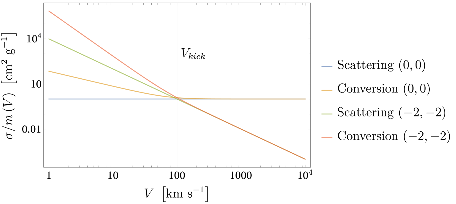
Figure 1: Cross sections for the power law indices $\left(a_{s},a_{c}\right)=\left(0,0\right)$ and $\left(-2,-2\right)$ with $\sigma_{0}=1\ \text{cm}^{2}\ \text{g}^{-1}$ and $V_{kick}=100\ \text{km}\ \text{s}^{-1}$. For $V>V_{kick}$, $\sigma_{c}$ behaves as a simple power law with an extra inverse power, i.e. while the power law index is $a_{c}$, the velocity dependence goes as $V^{a_{c}-1}$.

Particle interactions are modelled in the code using a Monte-Carlo method. Using the same implementation as presented in Todoroki & Medvedev (2019a), we assume that all collisions are rare and binary. The probability of interaction channel $ij\rightarrow i^{\prime}j^{\prime}$ within time step $\Delta t$ can therefore be modelled using the pair probability

$$P_{ij\rightarrow i^{\prime}j^{\prime}}=\left(\rho_{j}/m_{j}\right)\sigma_{ij\rightarrow i^{\prime}j^{\prime}}\left|{\bf V}_{j}-{\bf V}_{i}\right|\,\Delta t\,\Theta\text{,}$$ (5)

where, $\rho_{j}/m_{j}$ is the number density of target particles, $\sigma_{ij\rightarrow i^{\prime}j^{\prime}}$ is the cross section for the process $ij\rightarrow i^{\prime}j^{\prime}$, ${\bf V}_{j}-{\bf V}_{i}$ is the relative velocity of initial particles, and $\Theta$ is the same Heaviside function from Equation 1. In every time step, for each particle, from 10 to 38 nearest neighbours are identified as potential scattering partners, from which the scattering probabilities are calculated. A random number is generated to determine which, if any, scattering channels are chosen. If an interaction occurs, the final particle energy and momenta magnitude are calculated in the centre-of-mass frame, with energy injected or removed in an inelastic interaction if need be. The final directions of momentum are chosen at random (but still opposite to each other) in the centre-of-mass frame. Under the rare binary collision approximation, any interactions within a single time step involving more than two particles are rejected. In principle, particle masses must also be adjusted in an interaction. In practice, the mass degeneracy is much smaller than the mass resolution of a simulation. Therefore, the simulation particles are of equal mass, but are labelled with their state so that appropriate interactions take place.

2.2 Simulation Suites

We present new cosmological simulations utilizing the above 2cDM model. Two kinds of simulations were performed. $N$-body simulations are dark matter only (DMO) and evolve only under gravitation, while hydrodynamical simulations implement baryonic physics. Simulations are performed using the advanced hydrodynamical code Arepo (Vogelsberger et al., 2012b). Gravity is implemented using the same TreePM/SPH code as in GADGET-3 (Springel, 2005; Springel et al., 2008), while baryonic physics follow the IllustrisTNG model (Pillepich et al., 2018). IllustrisTNG is an improvement to the Illustris model (Vogelsberger et al., 2014a; Torrey et al., 2014), implementing subgrid baryonic physics processes including star formation and feedback, black hole formation and feedback, and gas enrichment.

Initial conditions were generated using the N-GenIC code using cosmological parameters from Planck Collaboration et al. (2016), where $\Omega_{m}=0.302$, $\Omega_{\Lambda}=0.698$, $\Omega_{b}=0.046$, $\sigma_{8}=0.83$, $n_{s}=0.97$, and $H_{0}=100h\ \text{km}\ \text{s}^{-1}\,\text{Mpc}^{-1}$ so that $h=0.6909$. We note that no modified transfer function was used to generate these initial conditions - we only consider the late time dynamics of 2cDM. In our fiducial set of simulations, we choose a periodic box with side length $L_{box}=3h^{-1}\,\text{Mpc}$ and a total particle count of $N_{part}=256^{3}$. For the DMO simulations this yields a mass resolution of $1.38\times 10^{5}\mathrm{M_{\odot}}$, while for the hydrodynamical simulations the mass resolutions are $1.17\times 10^{5}\mathrm{M_{\odot}}$ and $2.11\times 10^{4}\mathrm{M_{\odot}}$ for DM particles and gas cells respectively. All simulations have a gravitational softening length of $404\,\text{pc}$ at $z=0$, yielding a force resolution scale of $1.31\,\text{kpc}$. Additional simulations demonstrating how results converge with $L_{box}$ and $N_{part}$ are presented in Appendix A.

All simulations begin at $z=99$. All DMO simulations are evolved to $z=0$. We evolve hydrodynamical simulations to $z=2$, due to their computational cost. A follow-up paper discussing results found at $z=0$ is in preparation.

Substructures are identified within the simulation box using the Friends-of-Friends (FoF) and Subfind algorithms (Springel et al., 2001; Dolag et al., 2009). The FoF algorithm organizes particles into groups. Subfind further organizes particles by their gravitational boundedness. Each FoF group contains a largest main halo and can have many smaller subhalos.

DMO Simulations - Parameter Space Exploration

For this study, we choose explore the 2cDM parameter space of two power laws identified by Todoroki & Medvedev (2019b, 2022) as being both physically natural as well as consistent with observations. These have $\left(a_{s},a_{c}\right)=\left(0,0\right)$ and $\left(a_{s},a_{c}\right)=\left(-2,-2\right)$ respectively. Each is physically motivated: the $\left(0,0\right)$ model corresponds to $s$-wave scattering, while the $\left(-2,-2\right)$ model arises naturally from maximizing the conversion probability Medvedev (2014b). Todoroki & Medvedev (2019b, 2022) also demonstrate that for each model, $\sigma_{0}/m\sim 1\ \text{cm}^{2}\ \text{g}^{-1}$ and $\Delta m/m\sim 10^{-8}$ (corresponding to $V_{k}\approx 100\ \text{km}\ \text{s}^{-1}$) produce results consistent with observational constraints. We explore the 2cDM parameter space by varying $\sigma_{0}/m$ and $V_{kick}$ about these values for the two power laws using the same initial conditions. In particular, we vary $\sigma_{0}/m$ between $0.1$ and $10\ \text{cm}^{2}\ \text{g}^{-1}$ and $V_{kick}$ between $20$ and $200\ \text{km}\ \text{s}^{-1}$ each in logarithmic steps. We also performed a CDM simulation using this initial condition as a baseline to compare against.

Hydrodynamical Simulations

To study how the 2cDM model behaves in the presence of baryons, as well as to demonstrate the robustness of results, we perform a suite of simulations using 10 different initial conditions by varying the random seed in N-GenIC. For each initial condition, we perform 10 hydrodynamical simulations for each power law with fixed 2cDM parameters $\sigma_{0}/m=1\ \text{cm}^{2}\ \text{g}^{-1}$ and $V_{kick}=100\ \text{km}\ \text{s}^{-1}$. 10 CDM simulations were performed as a baseline to compare against. We also performed corresponding DMO simulations to highlight the effect of the baryons. An overview of structure formation under the 2cDM model displayed in Figure 2.

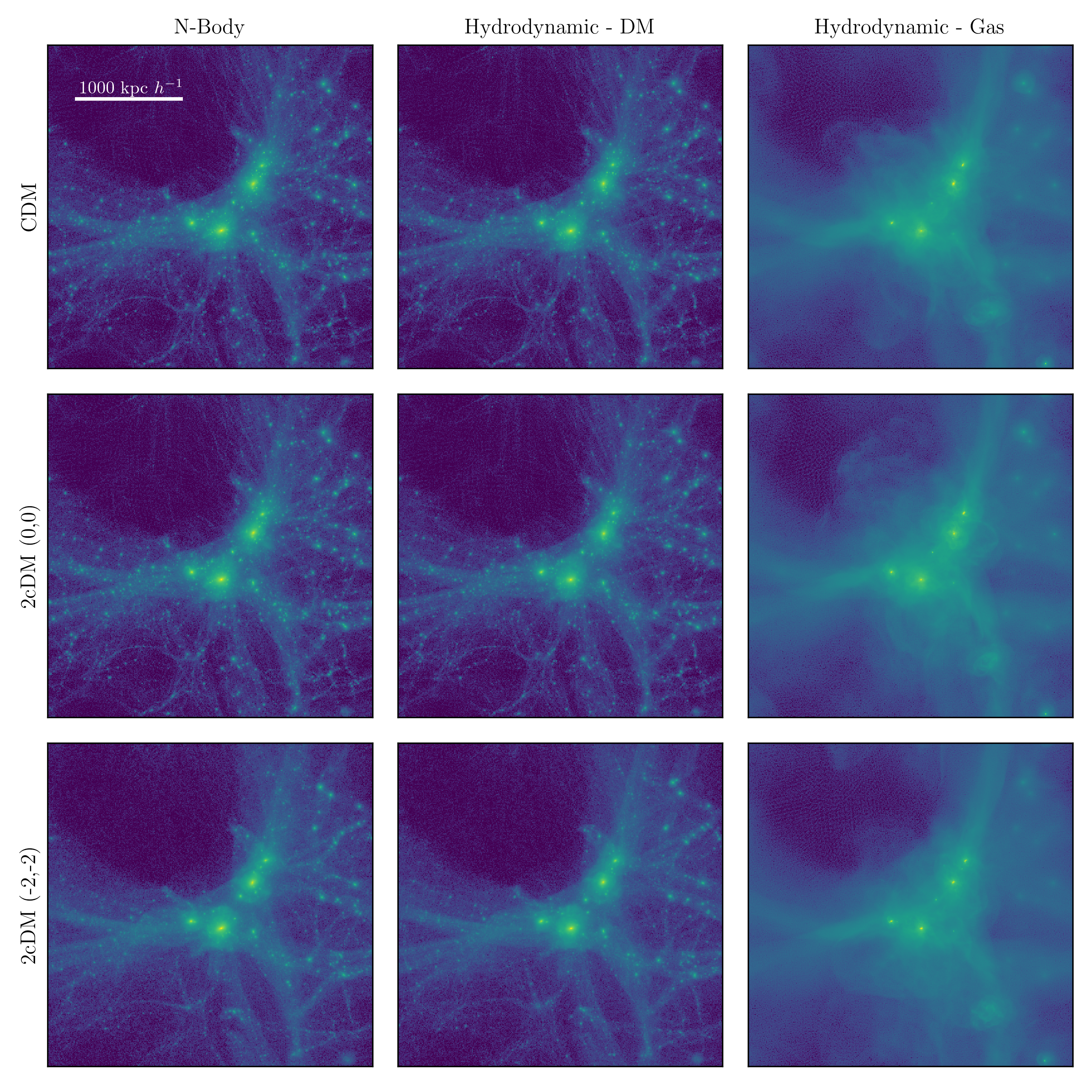
Figure 2: Halo formation within the 2cDM model. Each image shows the particle density via a histogram in the most dense slice of the $z$ coordinate. The top row is CDM, middle is the $\left(0,0\right)$ 2cDM model, and bottom is the $\left(-2,-2\right)$ 2cDM model. 2cDM simulations have 2cDM parameters $\sigma_{0}/m=1\ \text{cm}^{2}\ \text{g}^{-1}$ and $V_{kick}=100\ \text{km}\ \text{s}^{-1}$. The leftmost column is a DMO simulation, the middle column shows the DM particle density for the corresponding hydrodynamical simulation, and the rightmost column shows the gas particle density. Comparison by eye with CDM shows that both 2cDM models suppress small scale halo formation while keeping the large scale structure intact.

Data Products

For all simulations, we analyse three related summary statistics to determine the extent at which small scale structures are suppressed. The halo mass function (HMF) is the cumulative distribution of halo masses observed within each simulation box. It is related to the maximum circular velocity function (MCVF) via $V_{max}=\max\left\{\sqrt{GM\left(>R\right)/R}\right\}$. In principle, both measure the mass distribution of a halo population. While the HMF is more instructive in demonstrating the direct effect of 2cDM interactions, the MCVF is usually more readily measured in observation, as halo mass estimates are often reliant on direct measurements of velocity dispersions. To avoid counting spurious non-physical structures as well as avoid small-scale numerical effects, we only consider SubFind halos with $>30$ simulation particles, corresponding to halos with masses $\gtrsim 10^{6}\,\mathrm{M_{\odot}}$. In addition, we do not form structures with masses $\gtrsim 10^{11}\,\mathrm{M_{\odot}}$ due to the small box size.

A third metric we analyse is the one-dimensional dimensionless power spectrum $\Delta^{2}\left(k\right)$, which is a common statistical measure of density fluctuations with wavenumber $k$ (accordingly with characteristic size $\lambda=1/k$). $\Delta^{2}\left(k\right)$ is related to the ordinary power spectrum via $\Delta^{2}\left(k\right)=4\pi\left(2\pi\right)^{-3}k^{3}P\left(k\right)$. To calculate $P\left(k\right)$, consider fluctuations from the mean density $\bar{\rho}$

$$\delta\left(x\right)=\frac{\rho\left(x\right)-\bar{\rho}}{\bar{\rho}}.$$

From this, $P\left(k\right)=\left|\delta\left(k\right)\right|^{2}$, where $\delta\left(k\right)=\mathcal{F}\left\{\delta\left(\boldsymbol{x}\right)\right\}$ is the Fourier transform of $\delta\left(x\right)$.

Power spectra are common metrics in constraining alternative DM models. By surveying Lyman-$\alpha$ absorption in quasar spectra, one can obtain the density fluctuations in neutral Hydrogen at $z\sim 2-4$ and thereby estimate the density fluctuations in the matter density field (Hui & Gnedin, 1997; Croft et al., 1998). DM models that suppress or enhance the matter density field at some characteristic scale will produce a signature on the Ly-$\alpha$ forest, and therefore the matter power spectrum. This method has already been used to place large constraints on warm DM and decaying DM (Viel et al., 2013; Wang et al., 2013; Iršič et al., 2024; Dienes et al., 2022), and will only become more constraining as next-generation spectroscopic surveys release more data.

Power spectra were computed using the publicly available GenPK code (Bird, 2017). Numerically, the smallest scale one can probe before aliasing due to discretization occurs is the Nyquist wavenumber, $k_{Nyquist}=2\pi N^{1/3}/\left(2L\right)$. For our simulation suites, $k_{Nyquist}=286\ h\text{Mpc}^{-1}$. On large scales, accuracy is limited by the small number of modes with $\lambda\sim L_{box}$.

All three metrics give two important pieces of information: a scale at which suppression occurs and the degree of that suppression. To more easily discern the degree and scale, we present all quantities as ratios relative to CDM values in addition to the values themselves.

3 Results

3.1 Parameter Space Exploration

Variation of $V_{kick}$

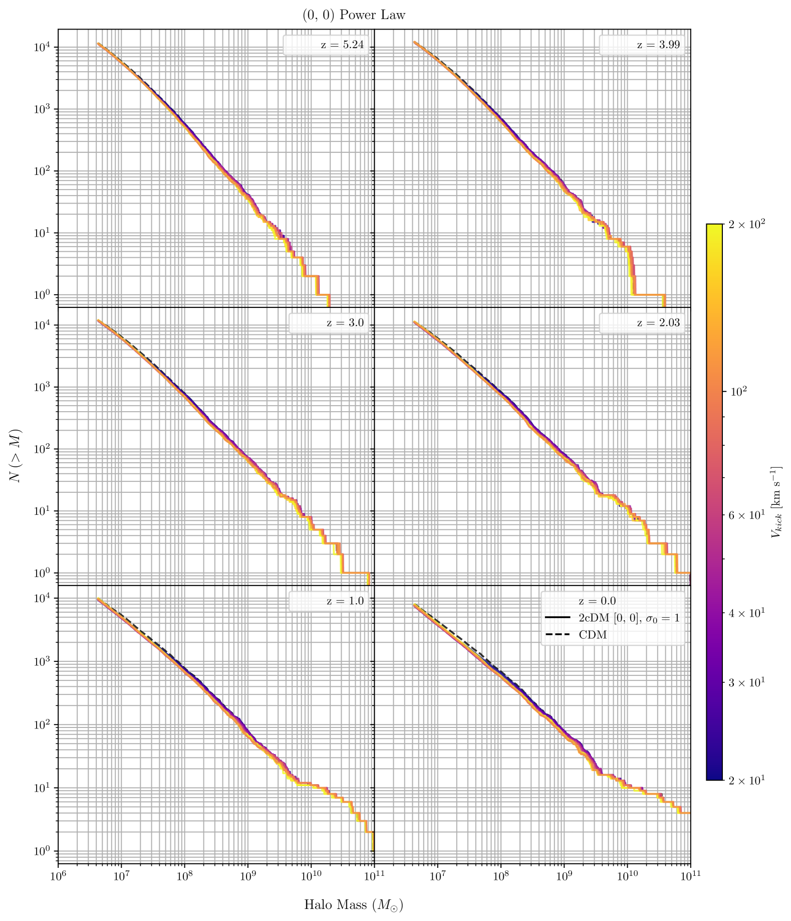
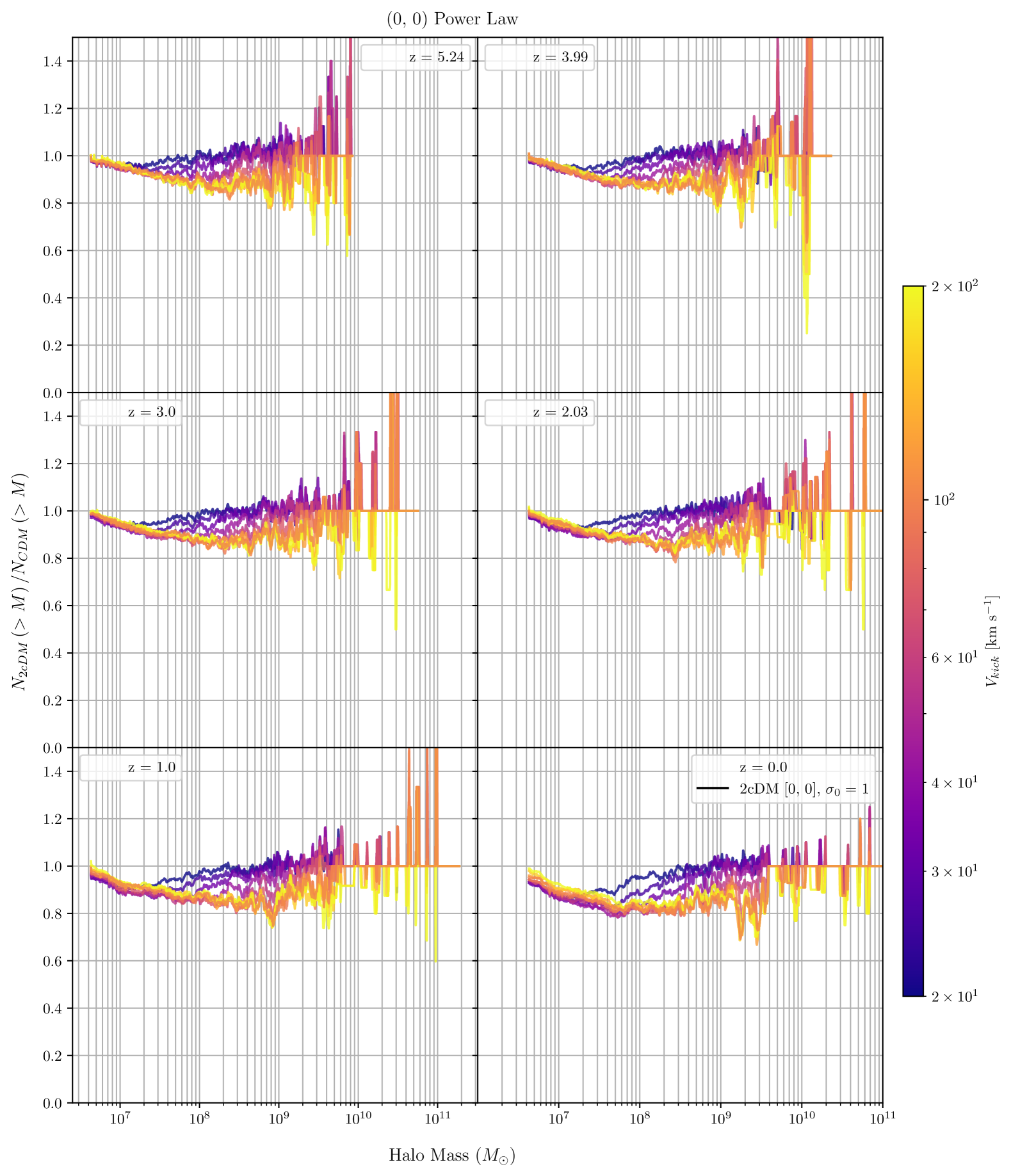
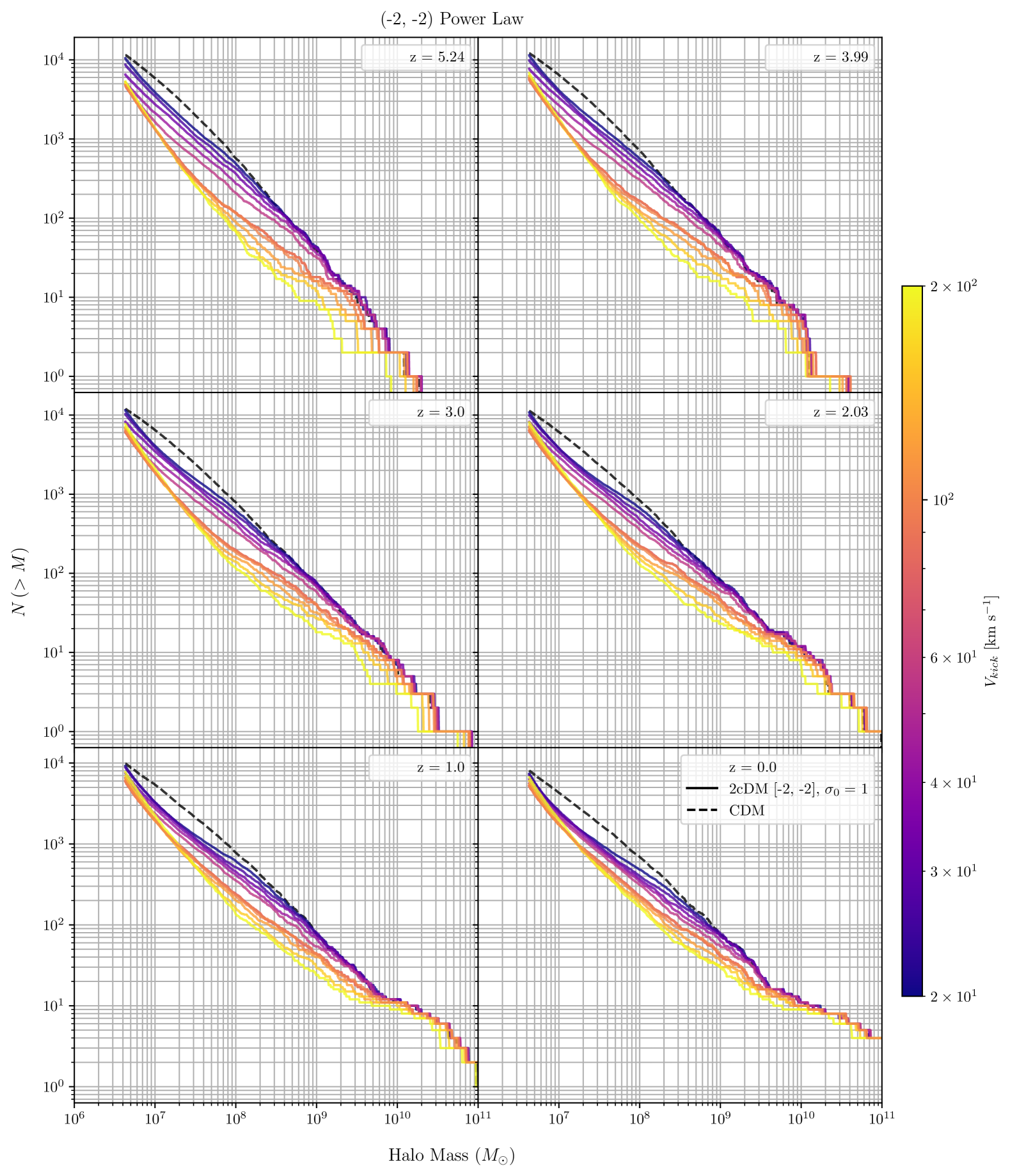
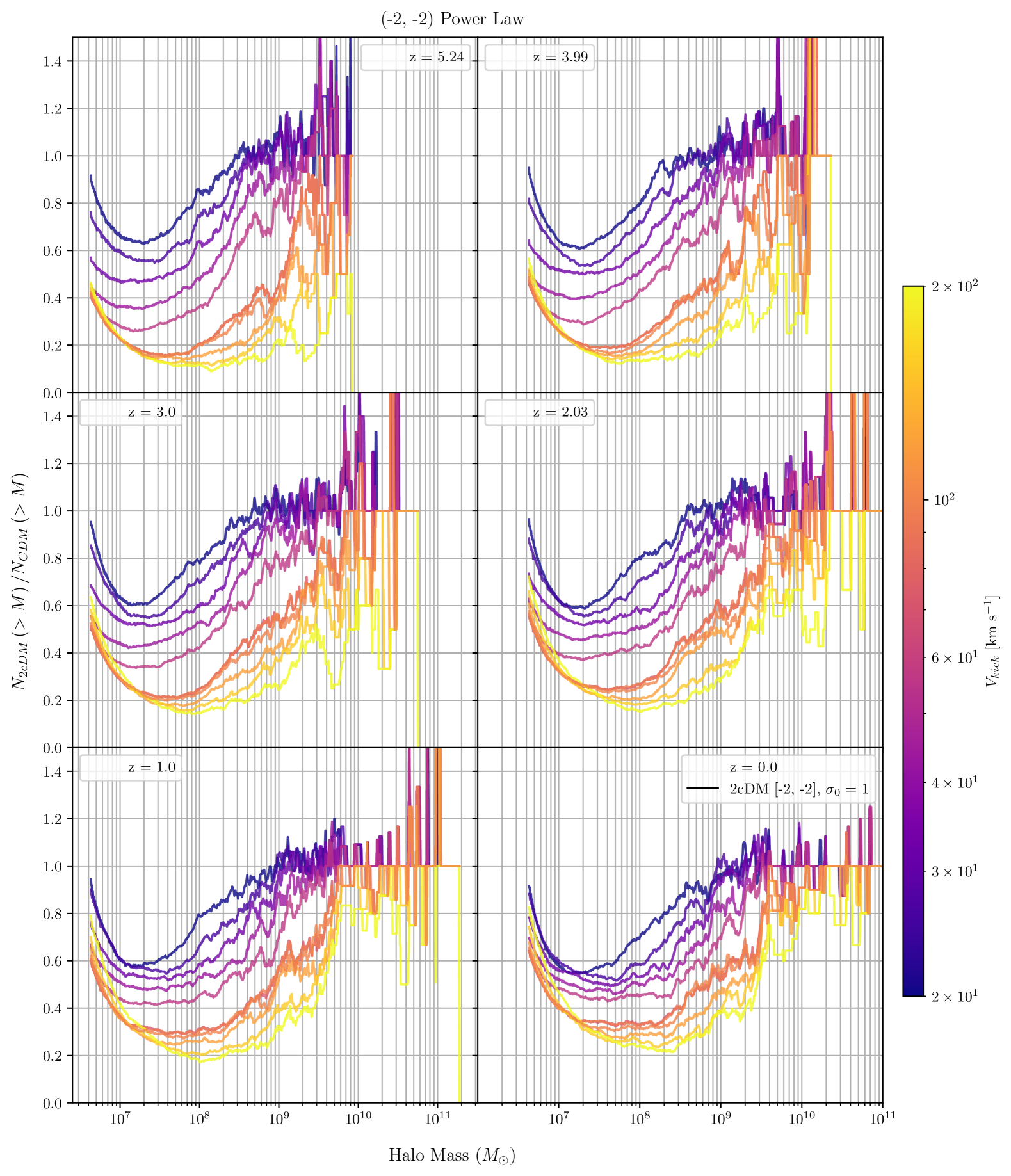
Figure 3: (Right Column) The halo mass functions for the 20 $V_{kick}$ variations, separated by power law. CDM is denoted by the dotted black line. Lines are coloured by the value of $V_{kick}$, with yellow representing larger values and blue representing smaller values. $\sigma_{0}$ is fixed at $1\ \text{cm}^{2}\ \text{g}^{-1}$ for these simulations. (Left Column) The ratio of 2cDM halo mass functions to the CDM halo mass function. The main effect of increasing $V_{kick}$ is to increase the energy injected in a conversion, thereby letting particles escape from halos more easily. This effect is clearly shown, where larger $V_{kick}$ leads to the suppression of more small structure and a shift in the peak amount of suppression to higher mass structures. The effect is less pronounced in the $\left(0,0\right)$ power law compared to the $\left(-2,-2\right)$ power law.

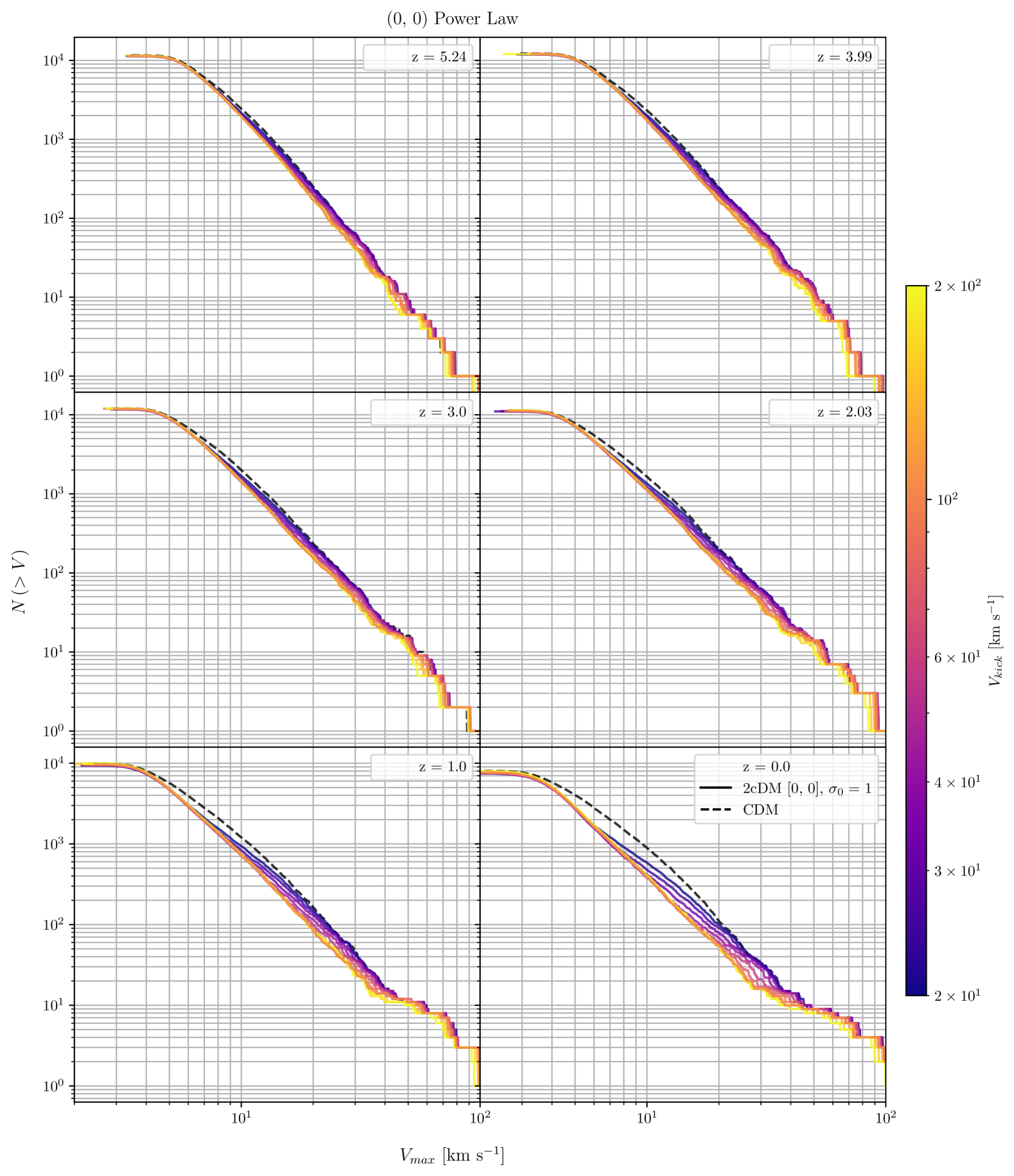
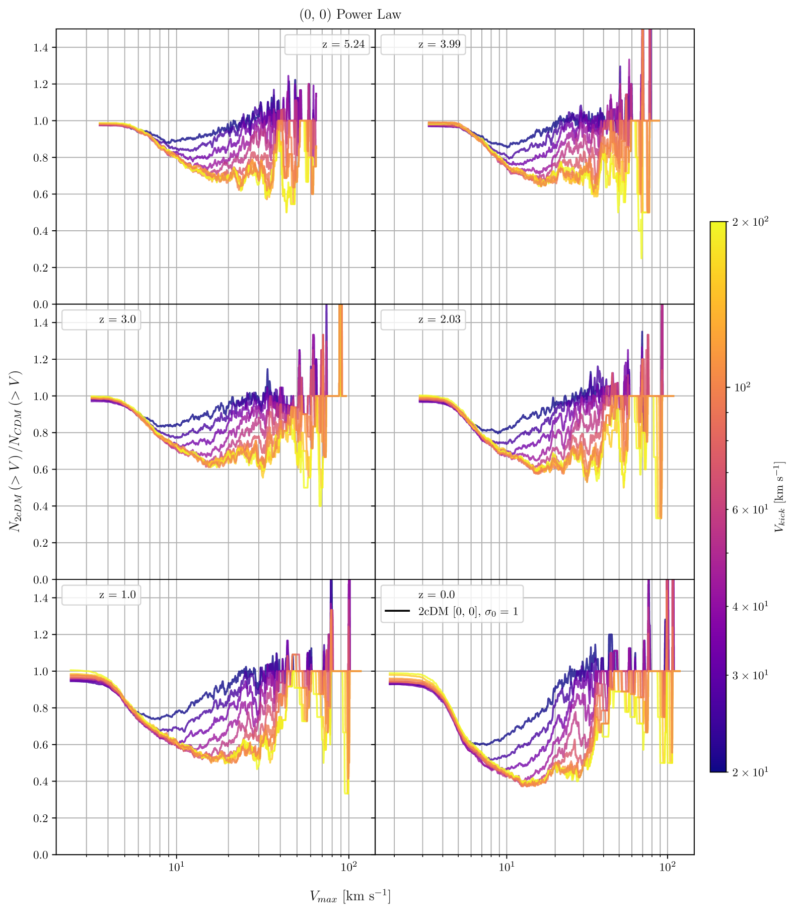
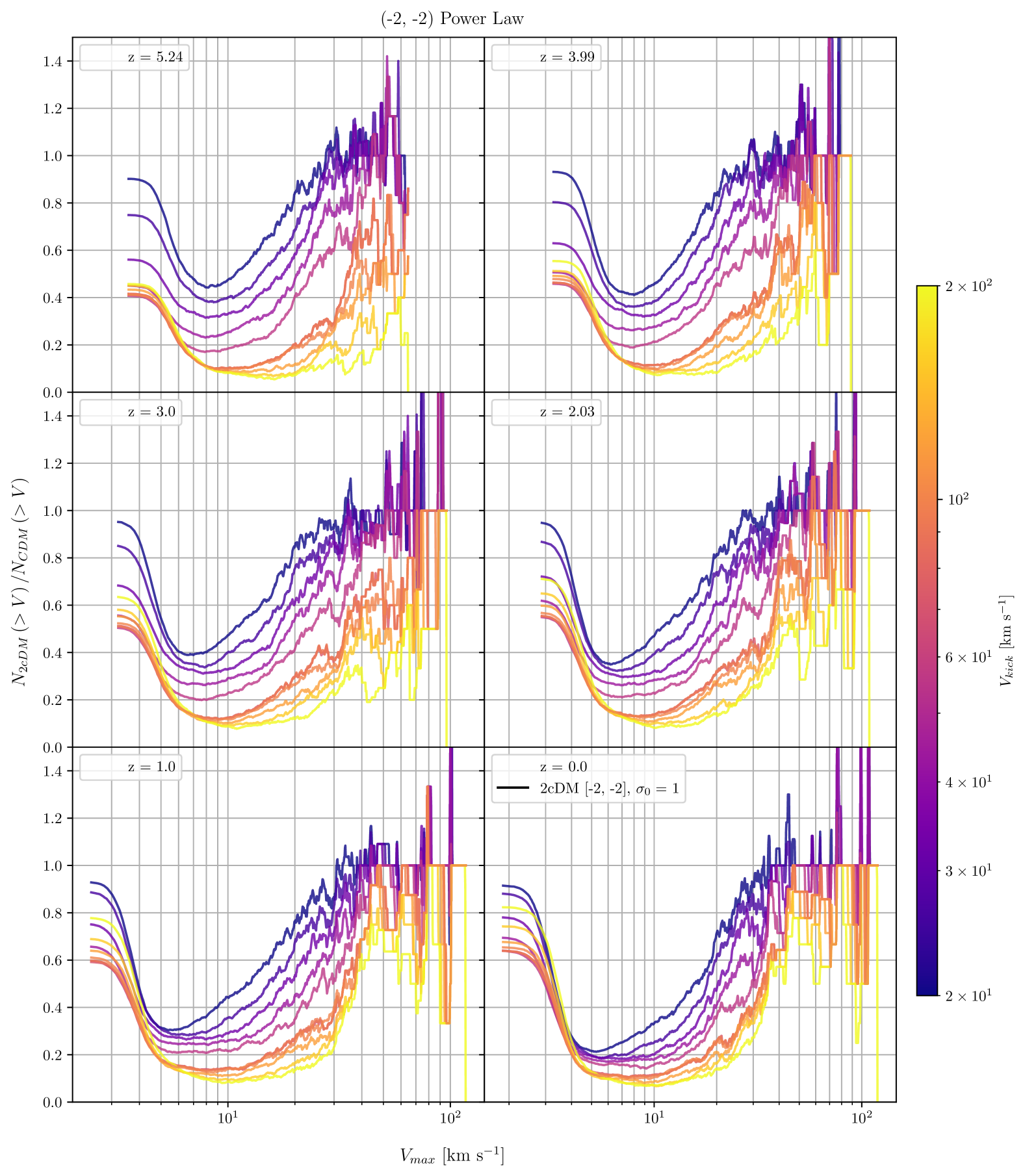
Figure 4: The $V_{max}$ function for the $V_{kick}$ variation suite. Labelling and colouring are identical to Figure 3. The effect of moving peak suppression to higher mass structures is now seen in both power laws. As expected, the $\left(-2,-2\right)$ power law shows a much higher degree of suppression, but the location of the peak is similar between both power laws.

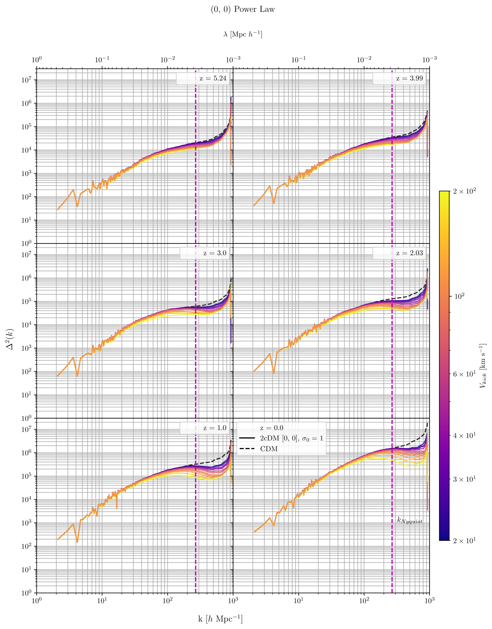
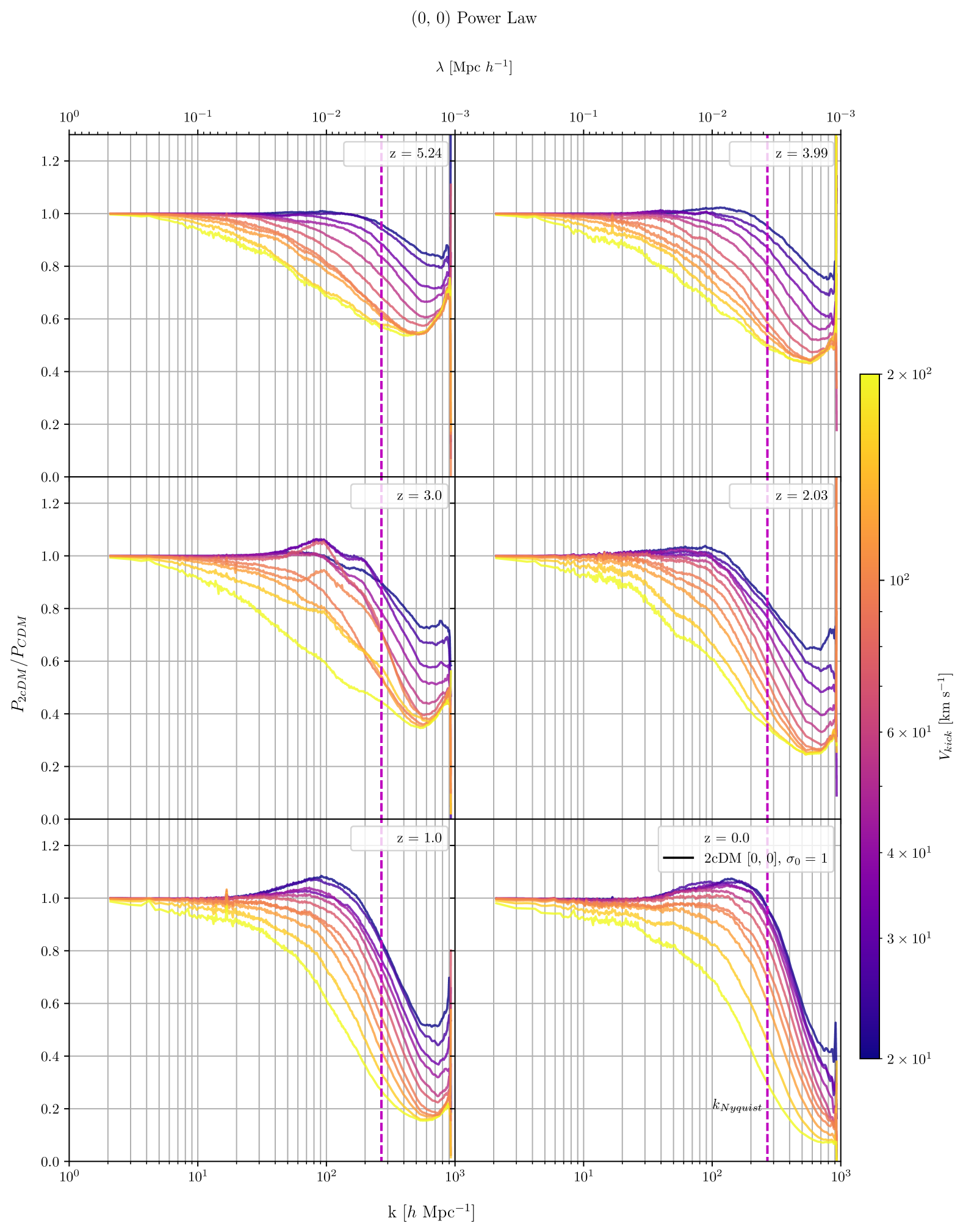
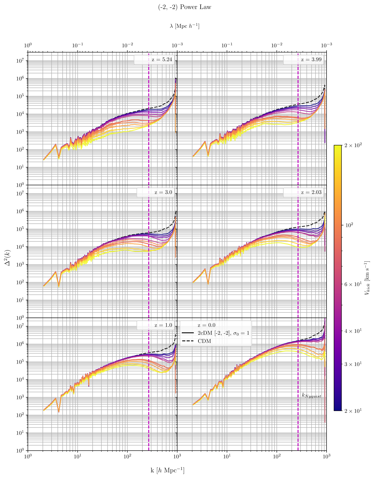
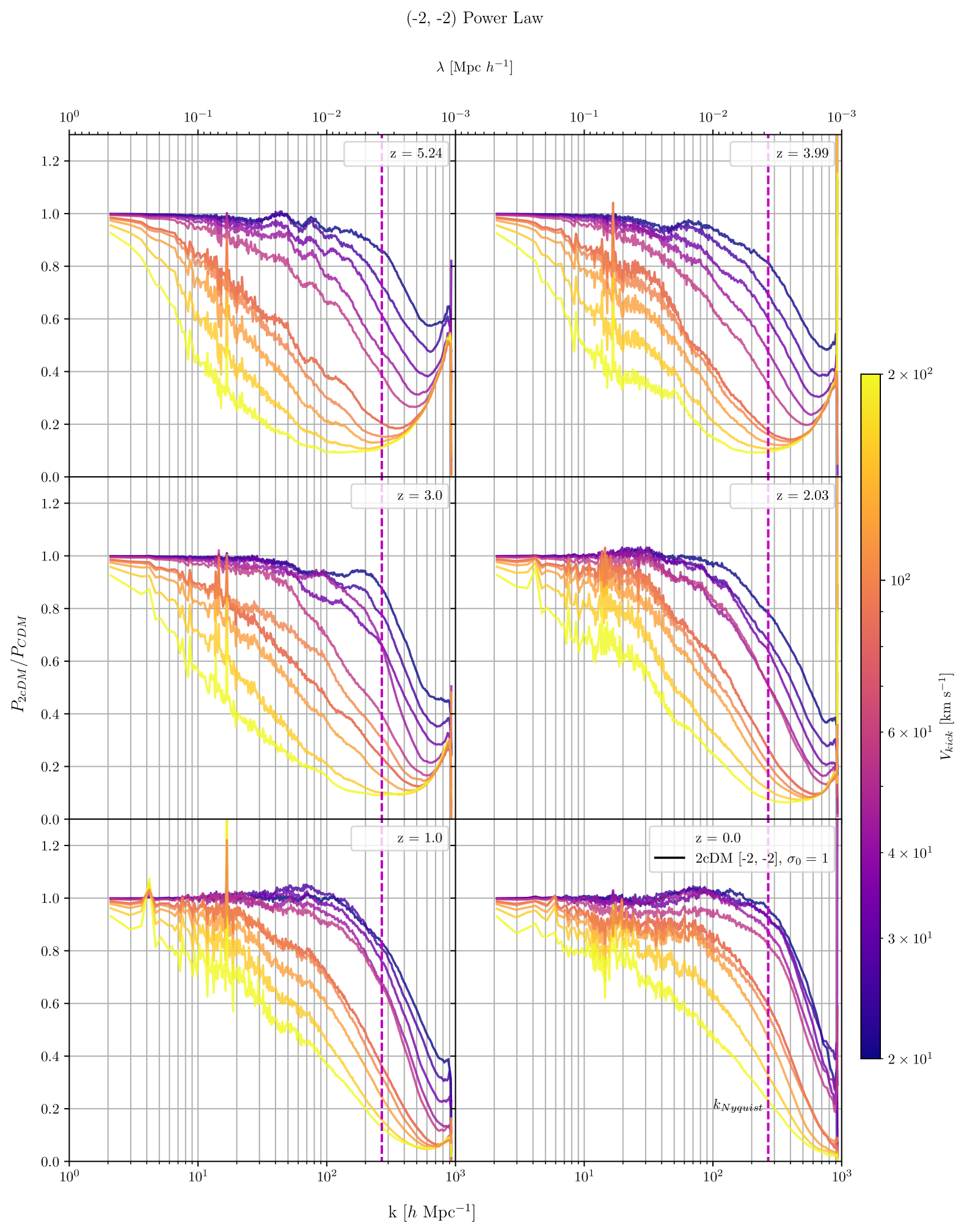
Figure 5: The dimensionless power spectrum for the $V_{kick}$ variation suite. Labelling and colouring are identical to Figure 3. Vertical lines denote the Nyquist wavenumber for the simulations. While the effects of the $\left(0,0\right)$ power law are less pronounced in halo statistics, the power spectra shows that even a modest $V_{kick}$ can produce $\sim 20\%$ suppression in the density distribution. As with the other statistics, the main effect of $V_{kick}$ is to move where suppression begins towards larger structures, that is higher $k$.

We vary $V_{kick}$ between $20$ and $200\ \text{km}\ \text{s}^{-1}$ in 10 logarithmic steps while keeping $\sigma_{0}$ fixed to $1\ \text{cm}^{2}\ \text{g}^{-1}$. Including the fiducial simulation with $10\ \text{km}\ \text{s}^{-1}$, we performed a total of 11 simulations per power law. The results are shown in Figures 3-5.

In Figure 3, we present the suppression in the HMF. For the $\left(0,0\right)$ power law, structure suppression only occurs with $V_{kick}\gtrsim 10\ \text{km}\ \text{s}^{-1}$, where the degree of suppression is $\sim 20\%$ relative to CDM at a scale of $M_{halo}\sim 10^{8}\,\mathrm{M_{\odot}}$. The $\left(-2,-2\right)$ power law produces a much higher degree of suppression at all $V_{kick}$ compared to the $\left(0,0\right)$ power law. The $\left(-2,-2\right)$ power law illustrates the main effect of $V_{kick}$ more clearly: increasing $V_{kick}$ changes where peak suppression occurs. As $V_{kick}$ increases, particles can escape more easily from more massive systems, thereby increasing the halo mass at which halo evaporation occurs.

This effect is most easily seen in the MCVF (Figure 4). For both power laws, it is clear that the effect of increasing $V_{kick}$ is to shift the suppression peak over towards higher $V_{max}$, while retaining a similar shape throughout. We also see that the effects on the MCVF can be different from the effects on the HMF. The $\left(0,0\right)$ power law has a growing degree of suppression across redshift between $30-60\%$ at $V_{max}\sim 11\ \text{km}\ \text{s}^{-1}$. The maximum degree of suppression for the $\left(-2,-2\right)$ power law is $\sim 90\%$ at $V_{max}\sim 10\ \text{km}\ \text{s}^{-1}$ across all redshift.

Power spectra are similarly affected (Figure 5). As $V_{kick}$ increases, the break between CDM and 2cDM power spectra moves to larger scales, i.e. towards larger $k$. Simulations with small $V_{kick}$ have enhancement or only small suppression above the Nyquist level. In the highest $V_{kick}$ cases, the $\left(0,0\right)$ power law shows suppression of up to $60\%$, while the $\left(-2,-2\right)$ power law a higher degree of suppression, up to $80\%$.

Variation of $\sigma_{0}$

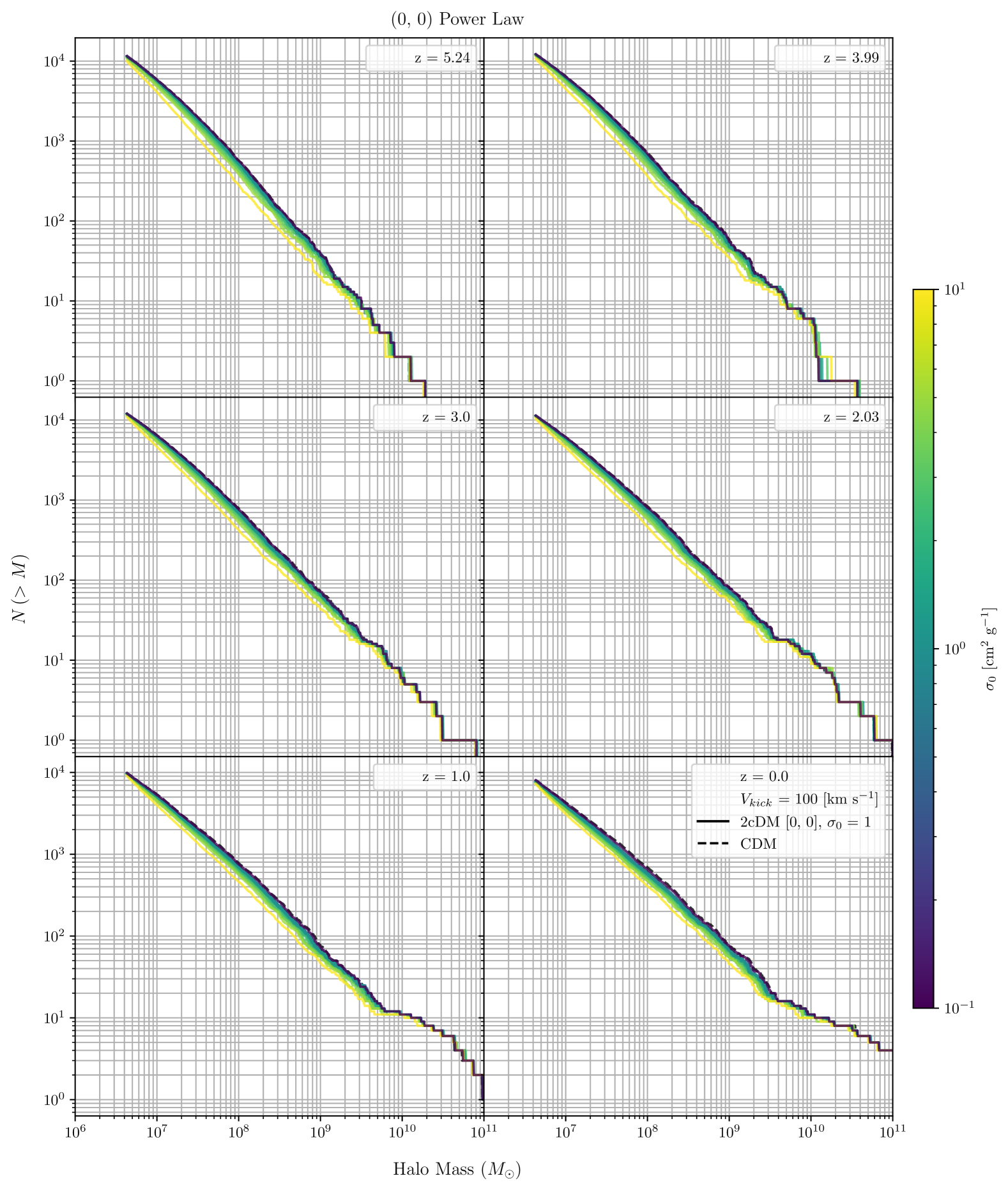
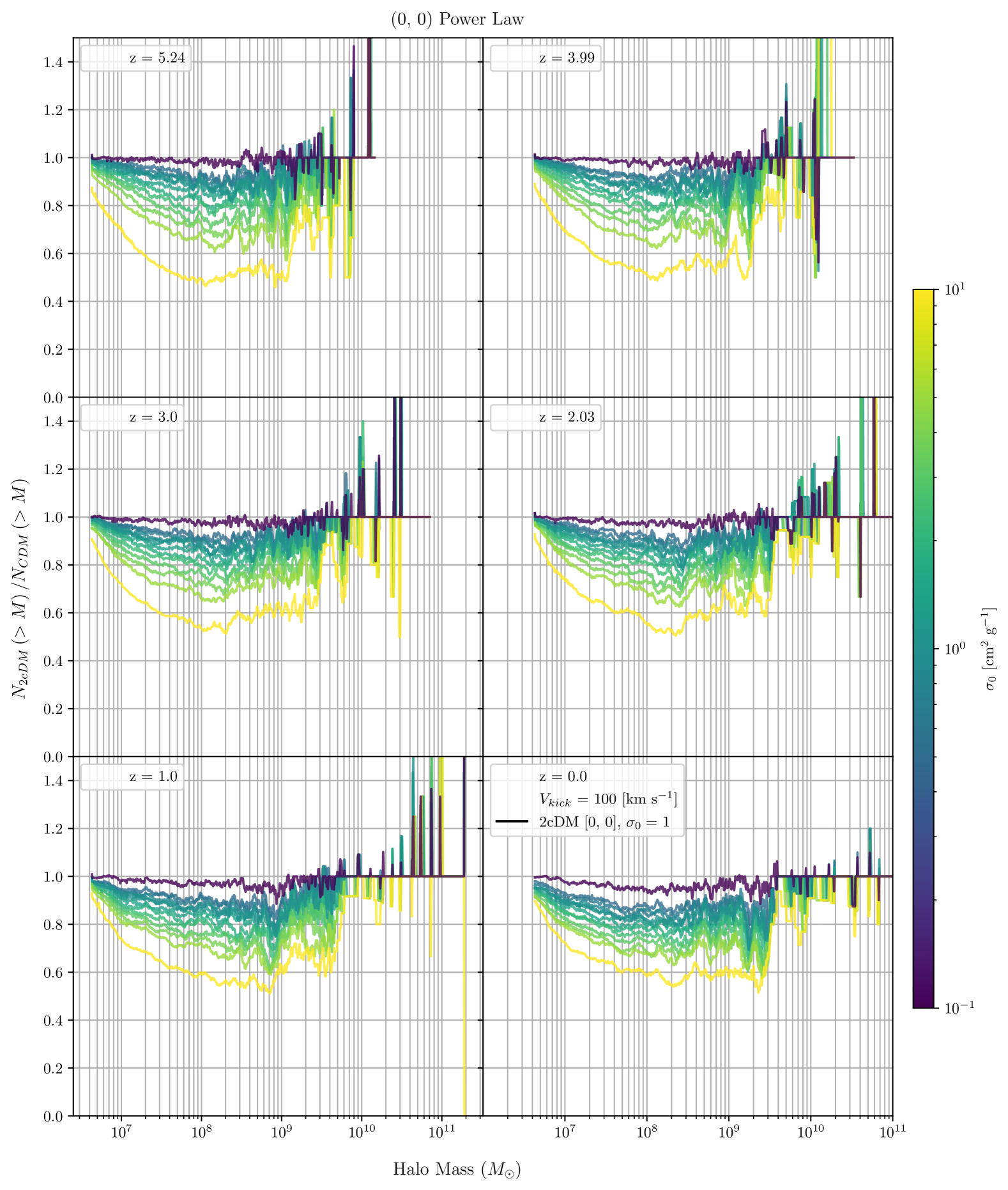
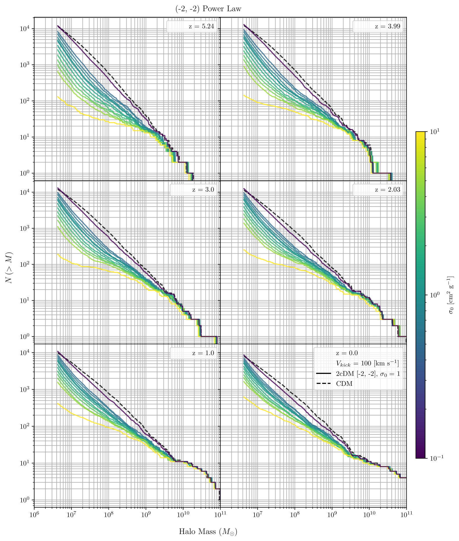
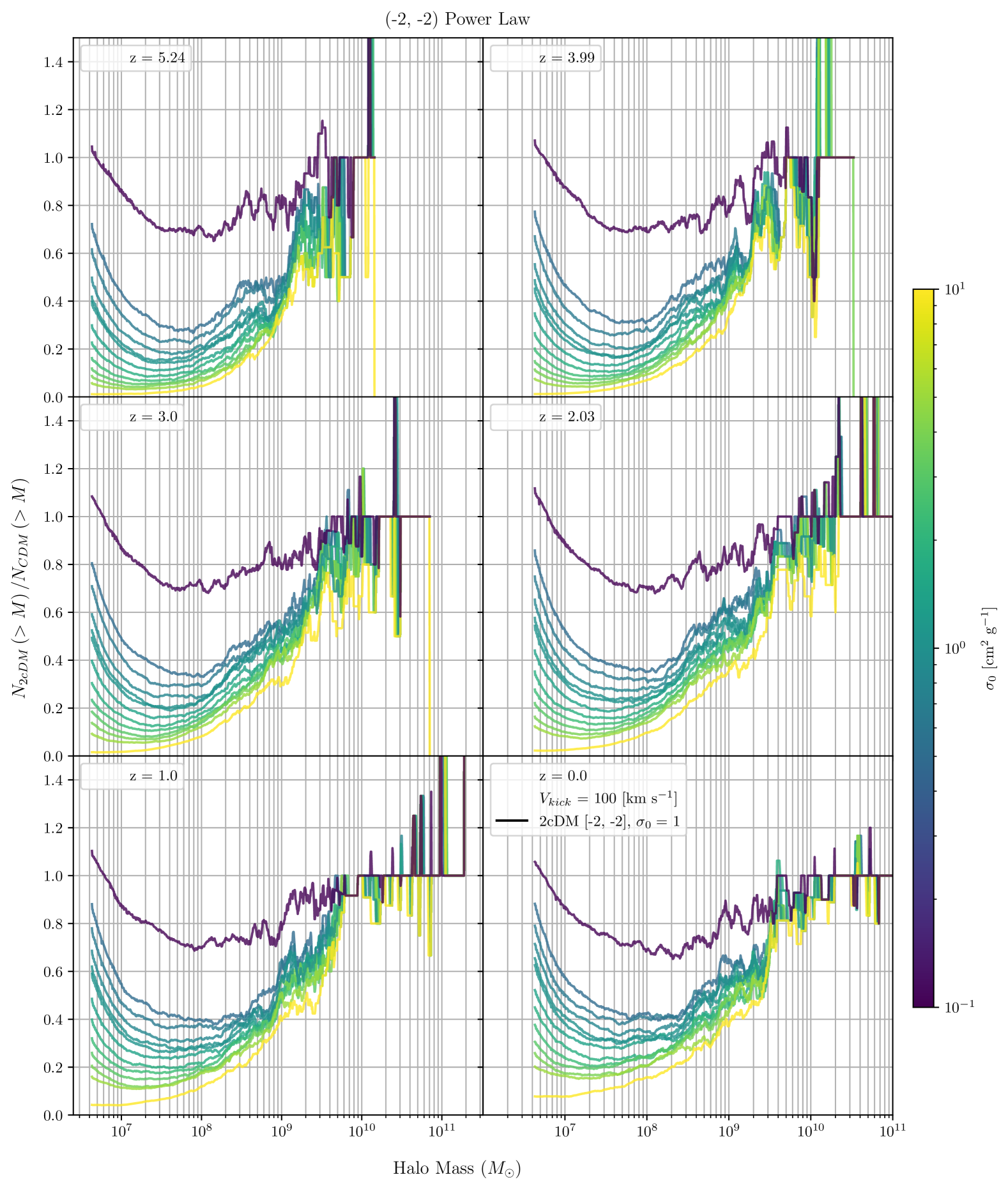
Figure 6: (Right Column) The halo mass functions for the 20 $\sigma_{0}$ variations, separated by power law. CDM is denoted by the dotted black line. Lines are coloured by the value of $\sigma_{0}$, with yellow representing larger values and blue representing smaller values. $V_{kick}$ is fixed at $100\ \text{km}\ \text{s}^{-1}$ for these simulations. (Left Column) The ratio of 2cDM halo mass functions to the CDM halo mass function. For both power laws, we see that the location of peak suppression remains the same. Only the degree of suppression is increased. In other words, the overall shape of the suppression curve remains the same, just deepened. This corresponds to the higher collision rate from increasing $\sigma_{0}$.

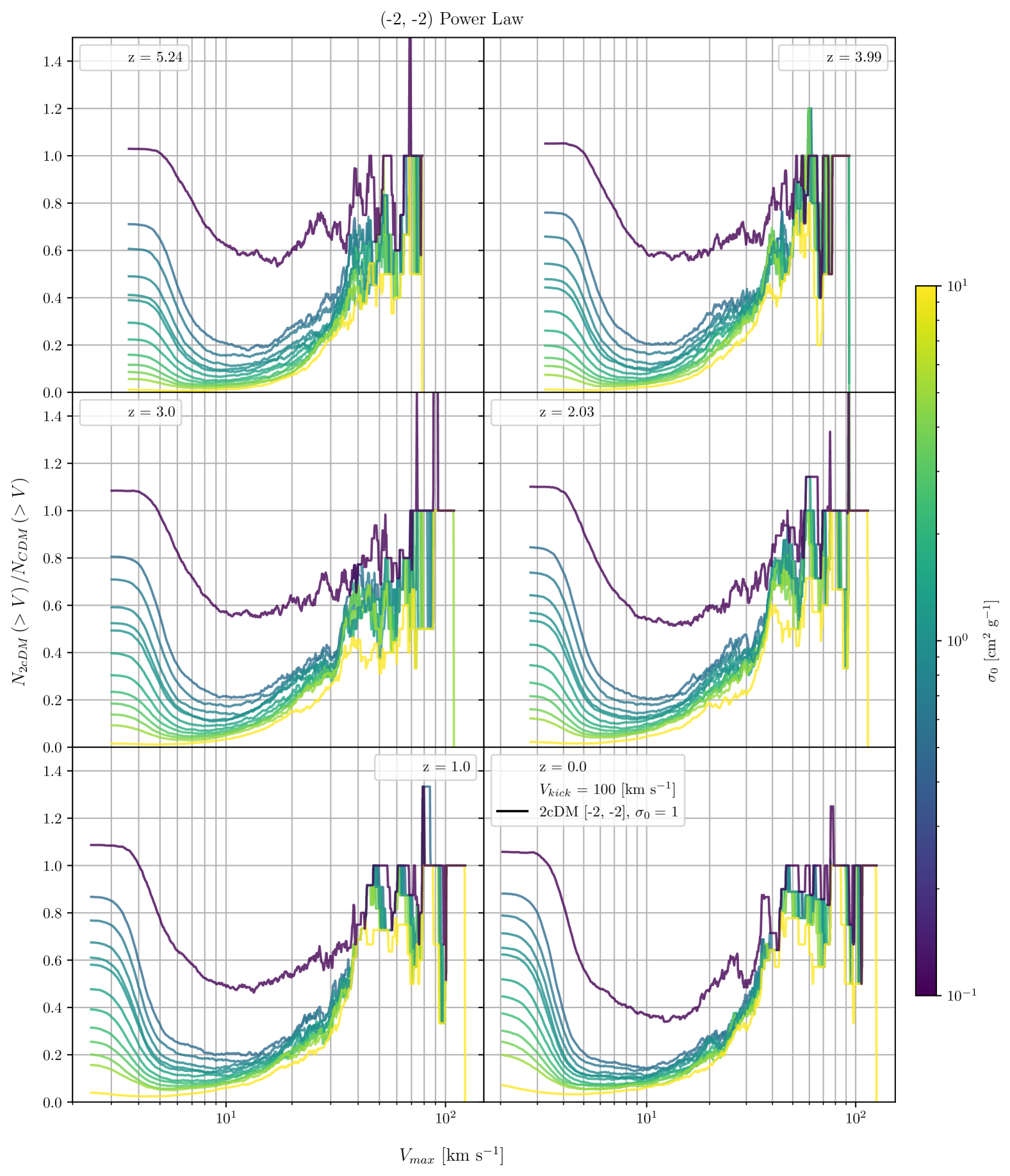
Figure 7: The $V_{max}$ function for the $\sigma_{0}$ variation suite. Labelling and colouring are identical to Figure 6. The same conclusion as in Figure 6 can be drawn here. The overall shape of the suppression curve remains the same, just deepened.

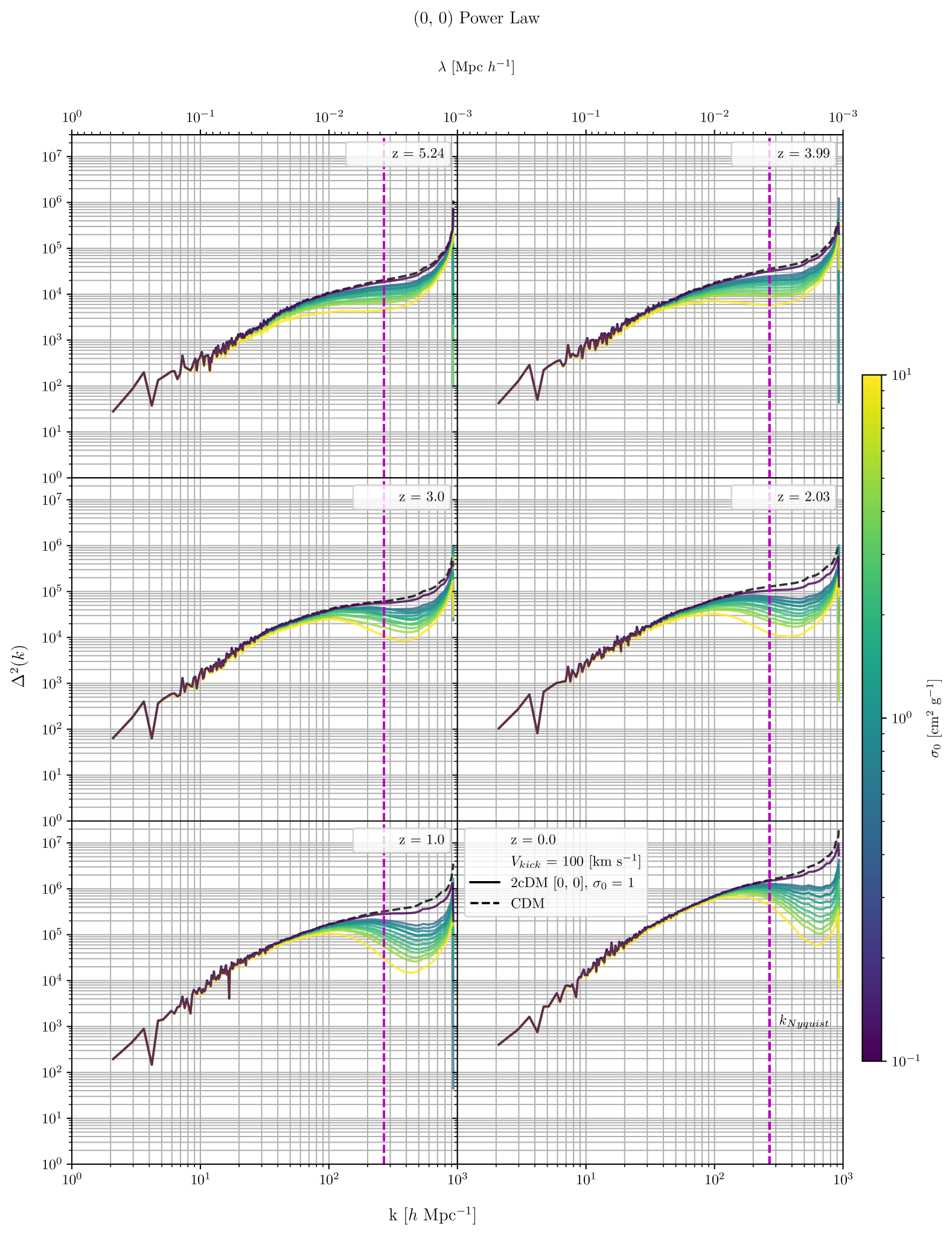
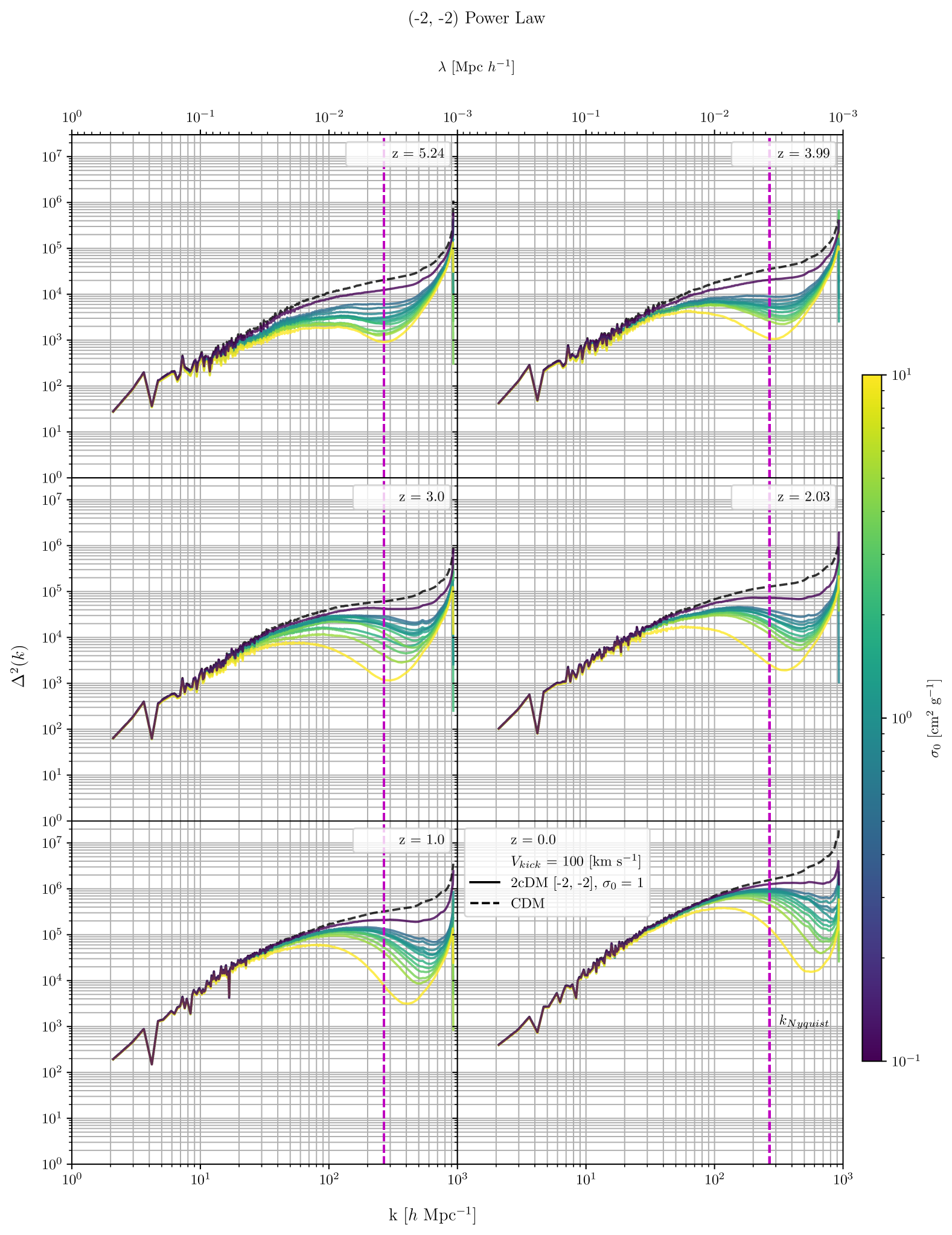
Figure 8: The dimensionless power spectrum for the $\sigma_{0}$ variation suite. Labelling and colouring are identical to Figure 6. Vertical lines denote the Nyquist wavenumber for the simulations. The $\left(0,0\right)$ power law demonstrates that the location of the break with CDM remains the same for all simulations and only the degree of suppression is changed. It is more difficult to make this same conclusion for the $\left(-2,-2\right)$ power law because the break occurs at such large scale for $V_{kick}=100\ \text{km}\ \text{s}^{-1}$.

We vary $\sigma_{0}$ between $0.5$ and $5\ \text{cm}^{2}\ \text{g}^{-1}$ in 10 logarithmic steps keeping $V_{kick}$ fixed to $100\ \text{km}\ \text{s}^{-1}$. In addition to the fiducial simulation with $\sigma_{0}=1\ \text{cm}^{2}\ \text{g}^{-1}$, as well as two additional simulations with $\sigma_{0}=0.1,10\ \text{cm}^{2}\ \text{g}^{-1}$, we performed a total of 13 simulations per power law. The results are shown in Figures 6-8.

The HMF suppression is displayed in Figure 6. With fixed $V_{kick}$, we see that the scale at which suppression occurs remains consistent between simulations and across redshift. Only the degree of suppression increases with increasing $\sigma_{0}$. The $\left(0,0\right)$ power law shows a consistent amount of suppression peaking around $M_{halo}\sim 10^{9}\mathrm{M_{\odot}}$, with a peak suppression of $\sim 40\%$. The $\left(-2,-2\right)$ power law becomes exponentially more collisional at small $V$ with increasing $\sigma_{0}$. In the most extreme cases, there is a severe reduction in structure across all scales, due to the difficulty in forming smaller seed structures to form larger ones. A similar story is shown for the MCVF (Figure 7) and $\Delta^{2}\left(k\right)$ (Figure 8).

In all examples, the when compared to CDM the overall shape of each curve remains similar, only deepening with increasing $\sigma_{0}$. This makes intuitive sense. $\sigma_{0}$ is responsible for setting the interaction rate, but $V_{kick}$ sets the amount of kinetic energy injected, thus setting the scale at which structures become suppressed.

3.2 Hydrodynamical Simulations

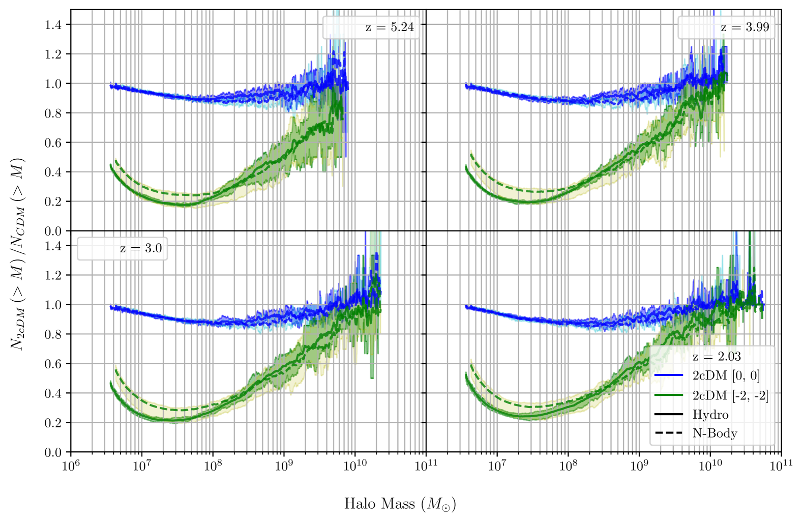
Figure 9: (Right) The halo mass functions for the fiducial suite of simulations between $z\sim 5-2$. Solid lines denote hydrodynamic simulations while dotted lines denote DMO simulations. Blue lines represent the $\left(0,0\right)$ model, green lines represent the $\left(-2,-2\right)$ model, and red lines represent CDM. Each line represents the average of 10 simulations. Shaded regions denote the $10$th to $90$th percentile. Fiducial simulations have fixed 2cDM parameters $\sigma_{0}/m=1\ \text{cm}^{2}\ \text{g}^{-1}$ and $V_{kick}=100\ \text{km}\ \text{s}^{-1}$. For clarity, shading for the DMO simulations are lighter than those for the hydrodynamical simulations. The full DMO variations are shown in Figures 13 - 15. (Left) Ratio of 2cDM halo mass functions to corresponding CDM halo mass functions. Low mass structures are suppressed to a similar degree to that presented in Figures 3 and 6 for the given 2cDM parameters. Baryons appear to provide slightly more suppression for the $\left(-2,-2\right)$ power law, however this is within the error bounds of the DMO simulations.

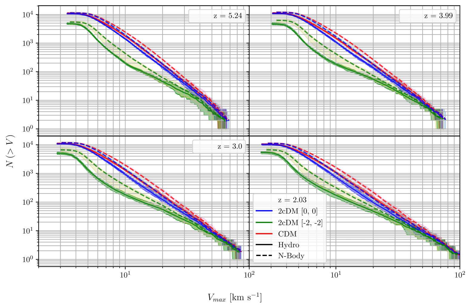
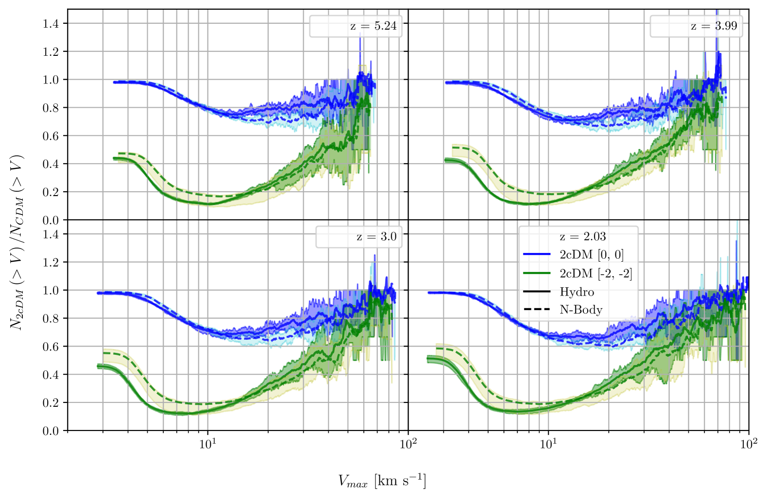
Figure 10: The $V_{max}$ functions for the fiducial suite of simulations. colouring is identical to Figure 9. Low mass structures are suppressed to a similar degree to that presented in Figures 4 and 7 for the given 2cDM parameters. Baryons provide significantly more suppression to systems with $V_{max}\lesssim 10\ \text{km}\ \text{s}^{-1}$ for the $\left(-2,-2\right)$ power law.

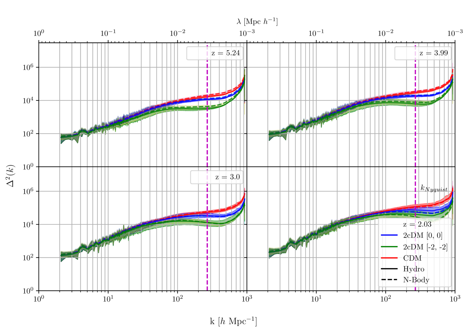
Figure 11: The dimensionless power spectra for the fiducial suite of simulations. Vertical lines denote the Nyquist wavenumber for the simulations. colouring is identical to Figure 9. Both power laws exhibit significant suppression relative to CDM at small scales across all redshifts. Results between $N$-body and hydrodynamic simulations are similar, with the $\left(0,0\right)$ power law perhaps showing some enhancement relative to its $N$-body counterpart.

To demonstrate the resilience of results to cosmic variation, we perform 10 hydrodynamical simulations per power law with different initial conditions. In addition to CDM and DMO counterparts, we performed a total of 60 simulations. As a reminder, these fiducial simulations use fixed 2cDM parameters of $\sigma_{0}=1\ \text{cm}^{2}\ \text{g}^{-1}$ and $V_{kick}=100\ \text{km}\ \text{s}^{-1}$. We present our results in Figures 9-11.

Because the HMF (Figure 9) and MCVF (Figure 10) are cumulative distributions, we can directly compare between hydrodynamic and DMO results. In both metrics, the $\left(0,0\right)$ power law shows remarkably similar results between hydrodynamic and DMO simulations. With our sample size, we can say the results are consistent up to cosmic variance. The $\left(-2,-2\right)$ power law have additional $10\%$ suppression at scales $M_{halo}\lesssim 10^{8}\,\mathrm{M_{\odot}}$ or $V_{max}\lesssim 10\ \text{km}\ \text{s}^{-1}$ compared to the DMO simulations. This difference is a most likely from baryonic feedback, as it appears outside the variance bounds of the DMO simulation.

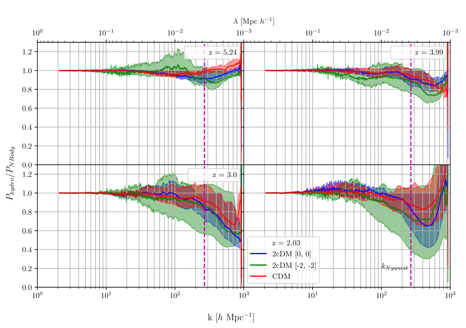
Figure 12: The ratio between power spectra for hydrodynamic and $N$-body simulations. Vertical lines denote the Nyquist wavenumber for the simulations. colouring is identical to Figure 9. Deviations from unity indicate hydrodynamic simulations producing different amounts of structure compared to $N$-body counterparts. Within the error bounds, all hydrodynamic simulations produce similar levels of suppression at small scales, though the deviation from unity is insignificant. Suppression between CDM and 2cDM simulations can therefore be mainly attributed to the modified DM physics.

We plot the power spectra for the fiducial simulations in Figure 11. There is differences between the hydrodynamic and DMO suites for both power laws and across all scales up to cosmic variance. Intuitively, this reflects the reduced role baryonic feedback plays at high redshift. We can further demonstrate that the effects are mainly due to the modified dark physics. In Figure 12 we plot the ratio between the hydrodynamic and DMO power spectra. In this comparison, effects from baryons are generally smaller, less than $20\%$ suppression at the Nyquist level, and are less consistent, seen in the much wider spread.

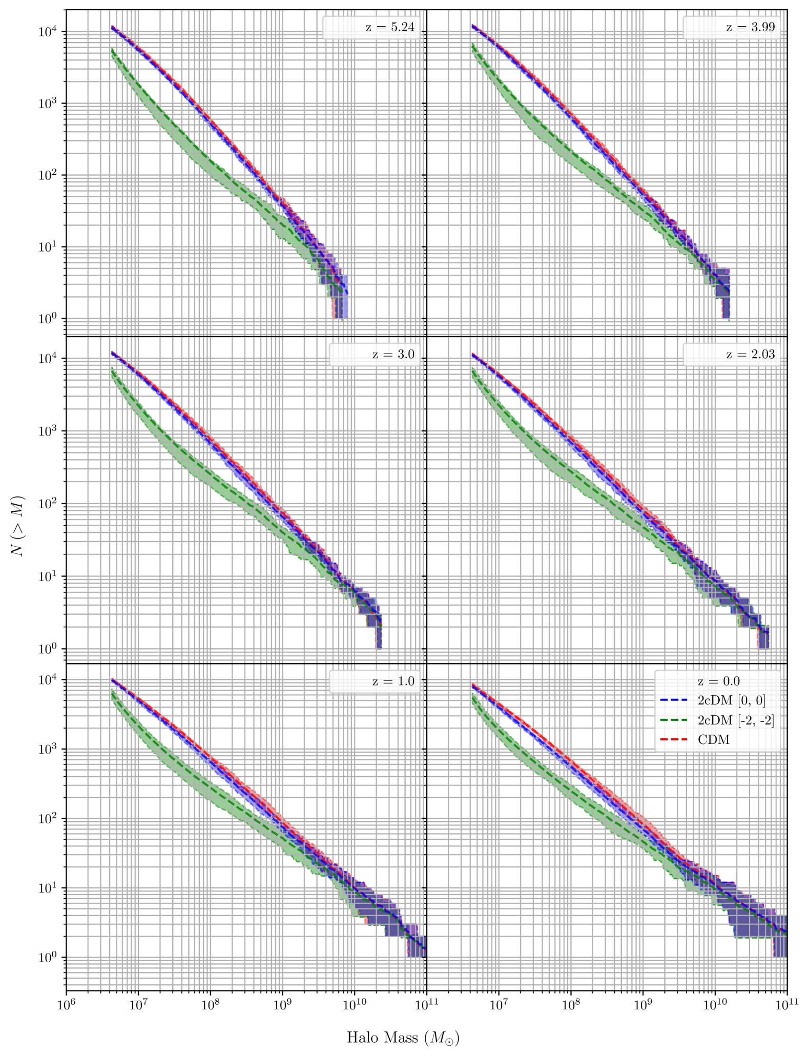
Figure 13: (Right) The halo mass function for the DMO suite of simulations from $z\sim 5-0$. Dotted lines denote that these are DMO simulations. As with Figures 9-11, blue lines represent the $\left(0,0\right)$ model, green lines represent the $\left(-2,-2\right)$ model, and red lines represent CDM. Each line represents the average of 10 simulations. Shaded regions denote the $10$th to $90$th percentile. Fiducial simulations have fixed 2cDM parameters $\sigma_{0}/m=1\ \text{cm}^{2}\ \text{g}^{-1}$ and $V_{kick}=100\ \text{km}\ \text{s}^{-1}$. (Left) Ratio of 2cDM halo mass functions to corresponding CDM halo mass functions. Simulations with the $\left(0,0\right)$ power law show low variation across all redshift while the $\left(-2,-2\right)$ power law shows variation of $\sim 10\%$, biased towards more suppression. Both power laws produce results consistent with the single parameter variations presented in Section 3.1.

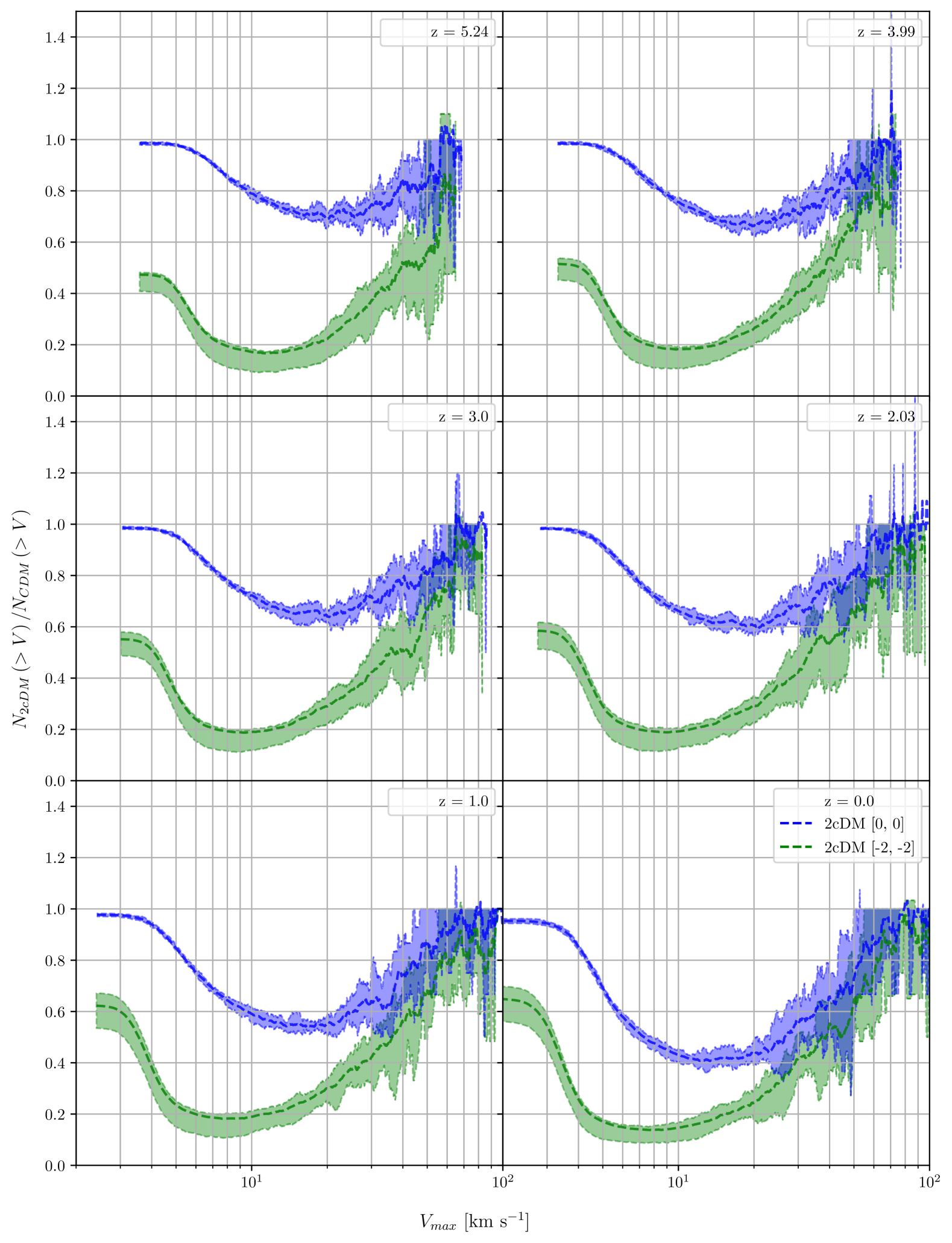
Figure 14: The $V_{max}$ functions for the DMO suite of simulations. The variation in the $V_{max}$ functions is generally less than that of the halo mass functions. Both power laws produce results consistent with the single parameter variations presented in Section 3.1.

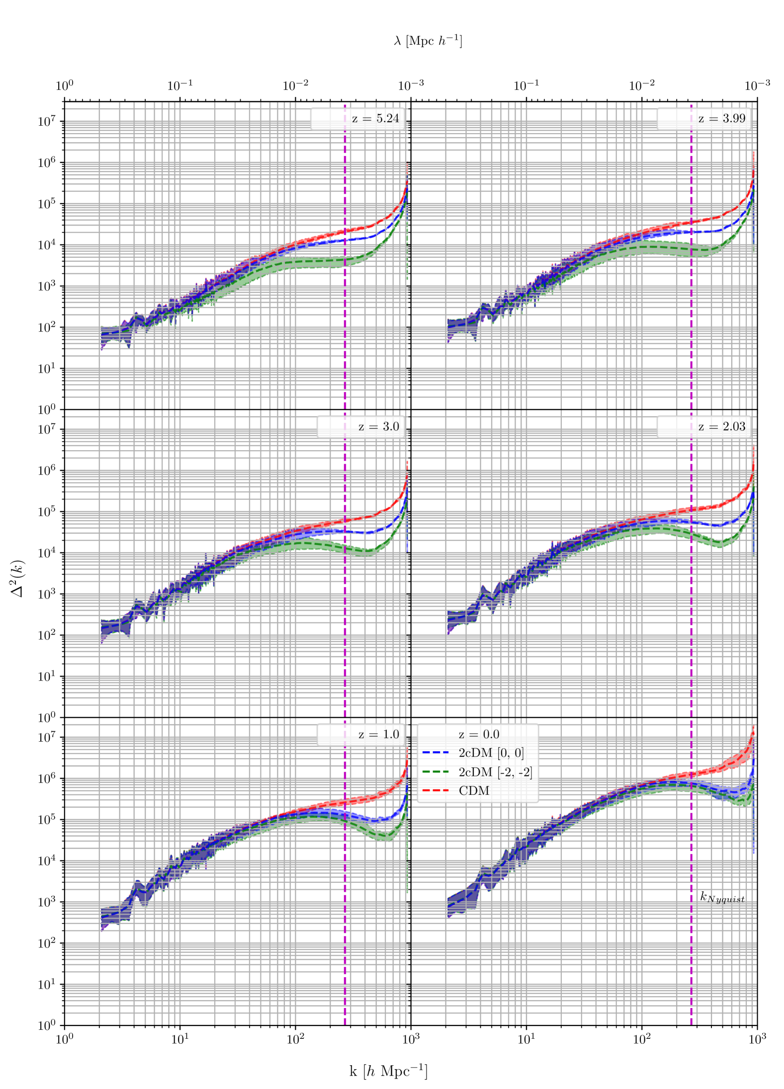
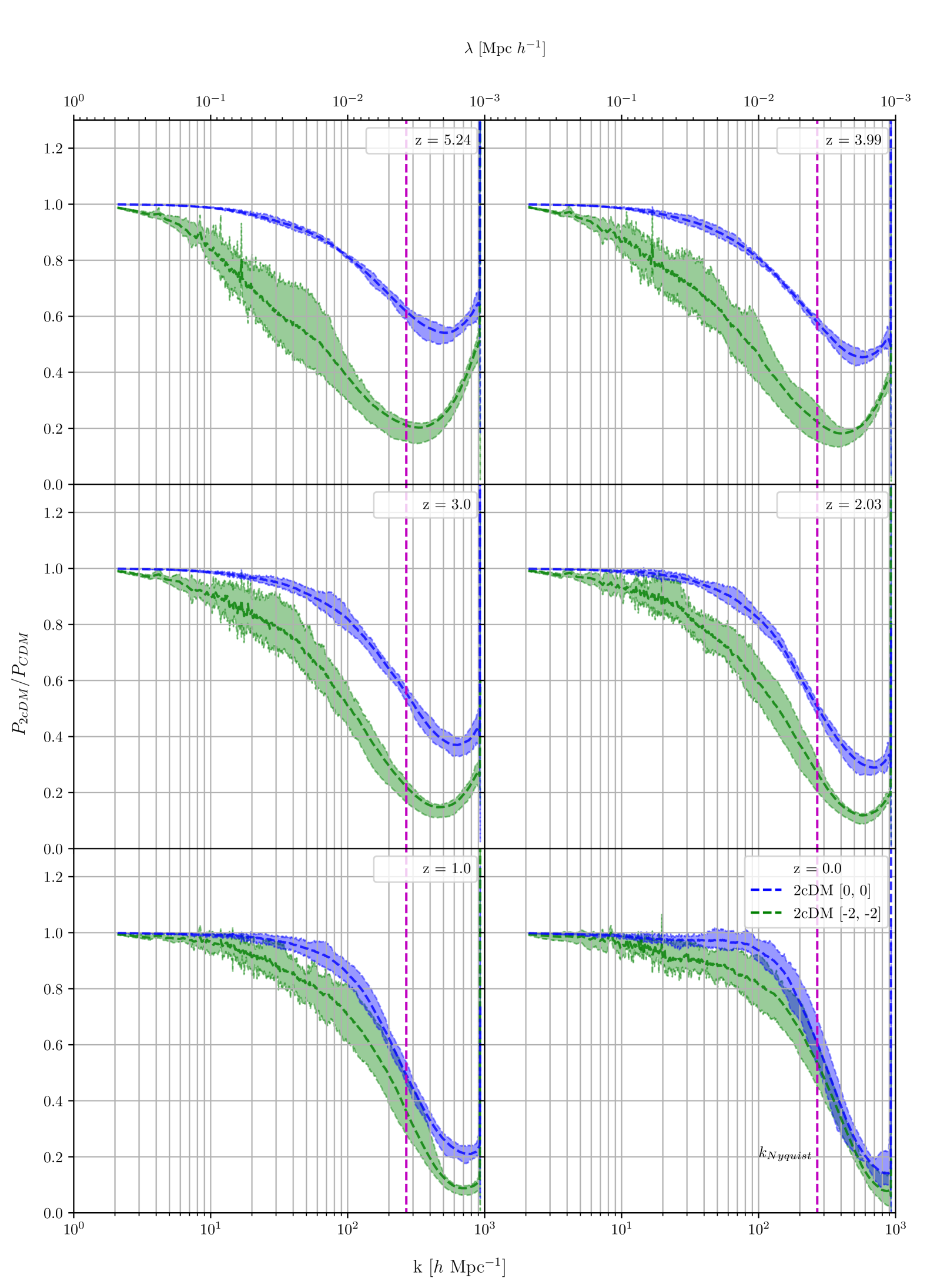
Figure 15: The dimensionless power spectra for the DMO suite of simulations. Vertical lines denote the Nyquist wavenumber for the simulations. Results as $z\rightarrow 0$ should not be expected to hold in the hydrodynamical case, as baryonic feedback becomes much more significant. Both power laws produce results consistent with the single parameter variations presented in Section 3.1.

For completeness, we plot all previously analysed metrics for the DMO suites in Figures 13-15. In DMO simulations, the suppression continues to $z=0$ with relatively low spread. This is consistent with results reported by Todoroki & Medvedev (2019a), though extends the analysis to a larger parameter range for the selected power laws. We anticipate that the low redshift results will not hold in hydrodynamic simulations, as the effects of baryonic feedback become larger in this regime.

4 Discussion

4.1 Degeneracies Between 2cDM and Baryonic Effects

Baryonic feedback is known to generally suppress power at scales $k\lesssim 2\text{Mpc }h^{-1}$ (van Daalen et al., 2011; Chisari et al., 2019; Schneider et al., 2019; van Daalen et al., 2020), and the effect is now well quantified across a range of cosmological and astrophysical parameters in the CAMELS suites (Villaescusa-Navarro et al., 2021; Gebhardt et al., 2024). As shown in Section 3, inelastic DM processes also provide suppression at those scales, so the effects are potentially degenerate. It is therefore crucial that we be able to distinguish baryonic effects from those of dark physics.

In CAMELS, the observed suppression over the parameter range is well constrained for IllustrisTNG, which we use in our simulations. In particular, we use the fiducial set of IllustrisTNG astrophysical and cosmological parameters, aligning ourselves with the CAMELS cosmic variance (CV) set of simulations. At scales of $k\gtrsim 2\text{Mpc }h^{-1}$, the ratio of hydrodynamic to $N$-body power spectra in the CAMELS TNG CV suite exhibits a "spoon" shape , where power is initially suppressed by up to $30\%$ before turning back towards $100\%$ (Villaescusa-Navarro et al., 2021). This decrease in the ratio of hydrodynamic to $N$-body power spectra indicates that hydrodynamic simulations tend to produce less structure than equivalent $N$-body simulations at those scales.

In Figure 12, we see that comparing our hydrodynamic to $N$-body simulations all simulations, both CDM and 2cDM, exhibit a small downturn at small scales, but the effect is insignificant up to cosmic variance. All hydrodynamic simulations appear to have similar amounts of substructure suppression relative to their $N$-body counterparts, indicating that the addition of baryons has a similar effect on small structure formation in both DM models. At $z\gtrsim 2$, it appears that the dominant effect on the power spectrum is therefore the modified dark physics.

However, degeneracies between baryonic physics and dark physics are still possible. The CAMELS Latin Hypercube (LH) set of simulations simultaneously varies astrophysical and cosmological parameters. In the TNG LH suite, the degree of suppression on the same scales is less constrained, with a maximum of $\sim 60\%$ and minimum of $\sim 10\%$, which can overlap with some of the more severe 2cDM models.

Similar results are seen when comparing to other baryonic physics prescriptions, such as SIMBA and ASTRID (Gebhardt et al., 2024). Under fiducial sets of parameters, the suppression from 2cDM is unique, but degeneracies appear once cosmological and astrophysical parameters are varied.

While it would be instructive to compare the other halo statistics, the HMF and MCVF, to results from CAMELS, the present suite of simulations unfortunately cannot. The choice of $L_{box}$ renders us unable to form halos of similar masses to the CAMELS boxes. However, as discussed in Section 2.1 and shown in Figure 16, 2cDM signatures are expected to stay at these small scales. Future studies utilizing Milky Way-like zoom-in suites, similar to those found in the DREAMS project (Rose et al., 2024) will help us to further understand the role astrophysical and cosmological parameters play at these small scales and how modified dark physics interacts with those parameters.

4.2 Application to Other DM Models

We now highlight potential applications of this computational approach to other DM models as well as its limitations.

Kong et al. (2015) proposed a similar two-component inelastic model, Boosted Dark Matter (BDM), with one of the main differences being a large mass difference and a primary annihilation process (in contrast to our low mass difference and primary conversion process). Kim et al. (2023) explored its early-time effects on the initial power spectrum. Kim et al. (2024) then used $N$-body CDM simulations with modified initial conditions to explore metrics similar to those presented in this work. The full consequences of the BDM model, including both early time and late time effects, can be readily implemented into this framework if the mass degeneracy and velocity dependent cross sections are known. Despite the large mass difference, realistic results could potentially be achieved through rare inelastic interactions or a low initial excited state fraction.

Other, more complicated inelastic DM models are possible. As we emphasized in Section 2, 2cDM is a special case of a generalized $N$-component flavour-mixed model. More interaction channels will inevitably lead to higher computational cost, as well as a higher probability of more-than-two particle collisions occurring within a time step, violating the rare binary collision approximation that we use. A highly-interacting DM acts more like a fluid, requiring a hydrodynamic approach to obtain accurate results. Work is already ongoing in adapting existing hydrodynamical codes to model fluid-like DM. Roy et al. (2023) implement such a model, atomic DM, in the GIZMO code. This computational approach applies on much different physical scales than the present framework. It would be interesting to investigate at which scale the binary collision approach becomes insufficient and a fully hydrodynamical implementation becomes necessary, and if a hybrid computational approach is practical or desirable.

5 Conclusions

We have presented the first suite of 2cDM simulations with IllustrisTNG physics. Our results indicate that baryonic physics does not significantly affect suppression due to 2cDM at $z\sim 5-2$. In this regime, suppression follows expectations from $N$-body simulations, suggesting this modified dark physics can be distinguished from degeneracies due to baryonic effects. Degeneracies can still exist as $z\rightarrow 0$. A future publication will follow these results down to $z=0$. to analyse how baryonic effects interact with modified DM physics deep into the nonlinear regime.

We have also demonstrated how two power laws, $\left(0,0\right)$ and $\left(-2,-2\right)$ , behave under a wide range of the 2cDM parameter space in $N$-body simulations. Our fiducial $N$-body and hydrodynamic simulations are self-consistent with these parameter space studies. Effort is ongoing to perform a similar parameter space exploration in hydrodynamic simulations.

It is known that uniform boxes struggle to simultaneously achieve a realistic Milky Way-like environment while also probing the scales necessary to observe 2cDM effects. Future studies will utilize zoom-in simulations to explore 2cDM in Milky Way-like systems more thoroughly.

Data availability

Data is available upon request.

Appendix A Tests of Numerical Convergence

Scaling With $L_{box}$

We perform single simulations with CDM and the 2cDM $\left(0,0\right)$ model with varying box sizes of $L_{box}=3,5,10\text{Mpc }h^{-1}$. The results for the same metrics discussed in Section 3 are displayed in Figures 16-19. Generally, the scale at which we see suppression relative to CDM is the same, though the larger boxes are less sensitive to the small scales where effects are the strongest.

Scaling With $N_{part}$

We perform single simulations with CDM and the 2cDM $\left(0,0\right)$ model with varying particle numbers of $N_{part}=128^{3},256^{3},512^{3}$. Results are only shown to $z=3$ due to the computational and storage cost of the $512^{3}$ set of simulations. Results generally align with each other, with the $128^{3}$ simulation exhibiting a high amount of noise due to small number of particles.

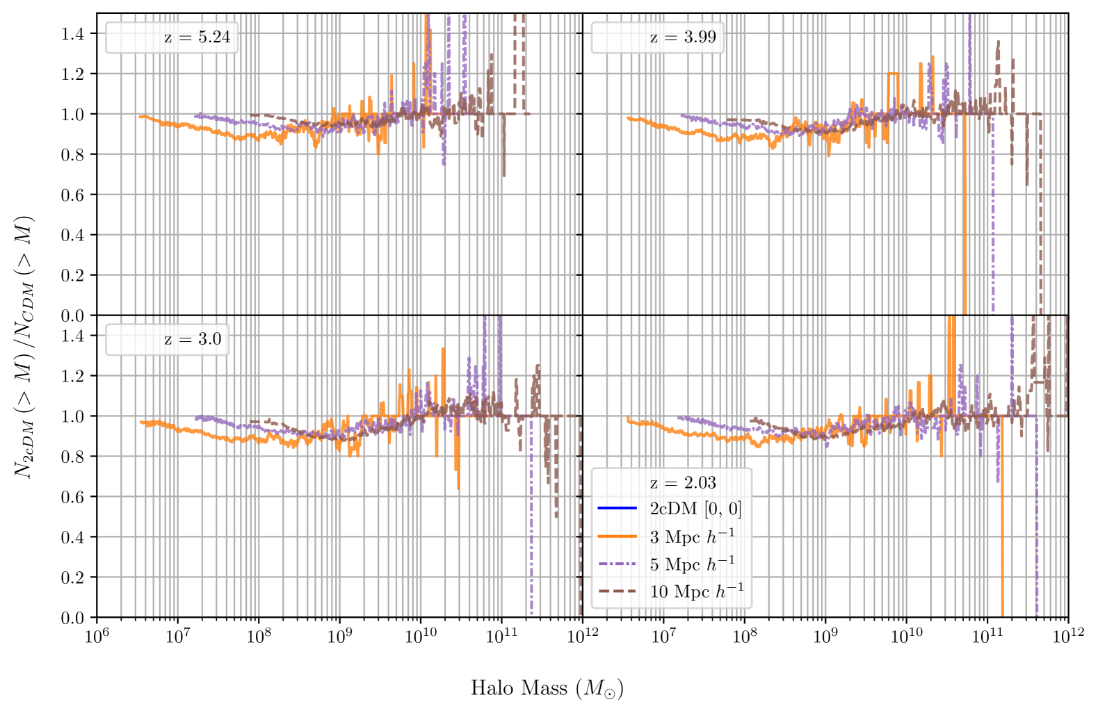
Figure 16: (Right) Comparing the halo mass function across simulations with varying $L_{box}$. Blue lines represent 2cDM simulations, while red lines represent CDM simulations. Solid lines correspond to the fiducial box size of $3\text{Mpc }h^{-1}$. Dash-dotted and dashed lines correspond to box sizes of $5\text{Mpc }h^{-1}$ and $10\text{Mpc }h^{-1}$ respectively. All simulations presented here are hydrodynamic. (Left) The ratio between 2cDM and CDM halo mass functions. Lines are coloured by box size.

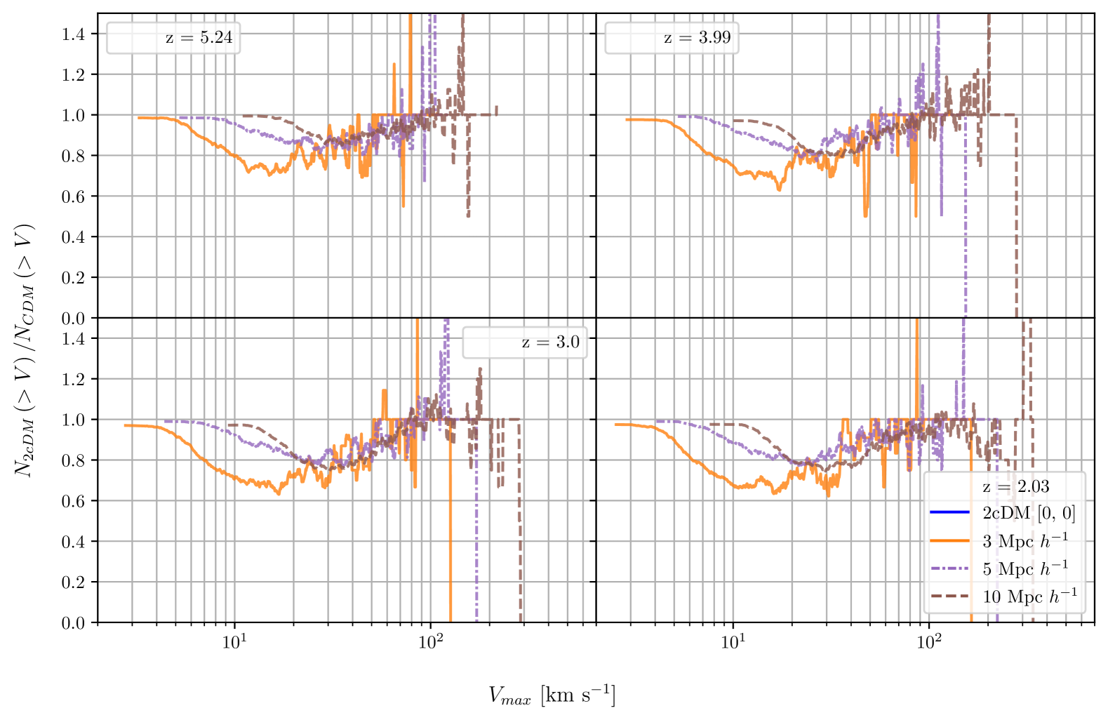
Figure 17: The $V_{max}$ functions for the $L_{box}$ scaling test. colouring is identical to Figure 16.

Figure 18: The dimensionless power spectra for the $L_{box}$ scaling test. Vertical lines denote the Nyquist wavenumber for the simulations. We note that the enhancement seen in the power spectra lie within the error bounds of our fiducial simulations. colouring is identical to Figure 16. Larger boxes at the same particle number cannot resolve smaller structures as well due to coarser mass and force resolutions. Box size does not appear to affect results significantly. Trends established below the Nyquist level of the largest boxes are followed well by the smaller boxes.

Figure 19: The ratio between power spectra for hydrodynamic and $N$-body simulations for the $L_{box}$ scaling test. Box size appears to have little effect on the convergence of results on scales greater than the largest $\lambda_{Nyquist}$.

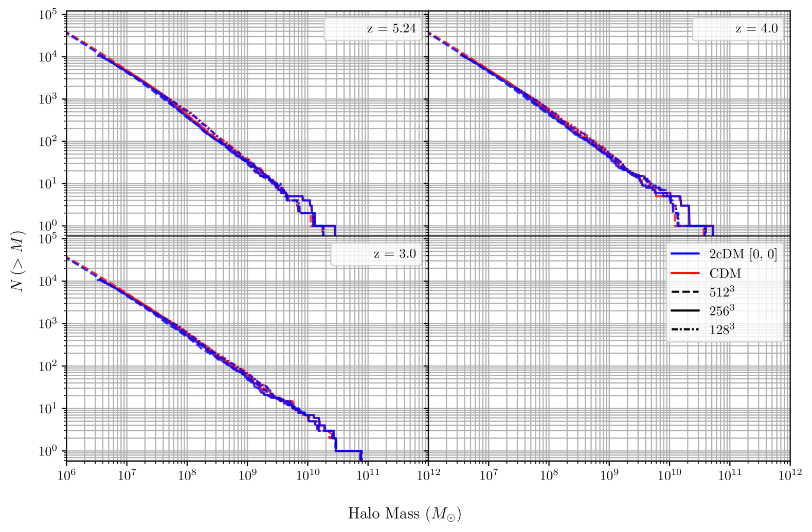
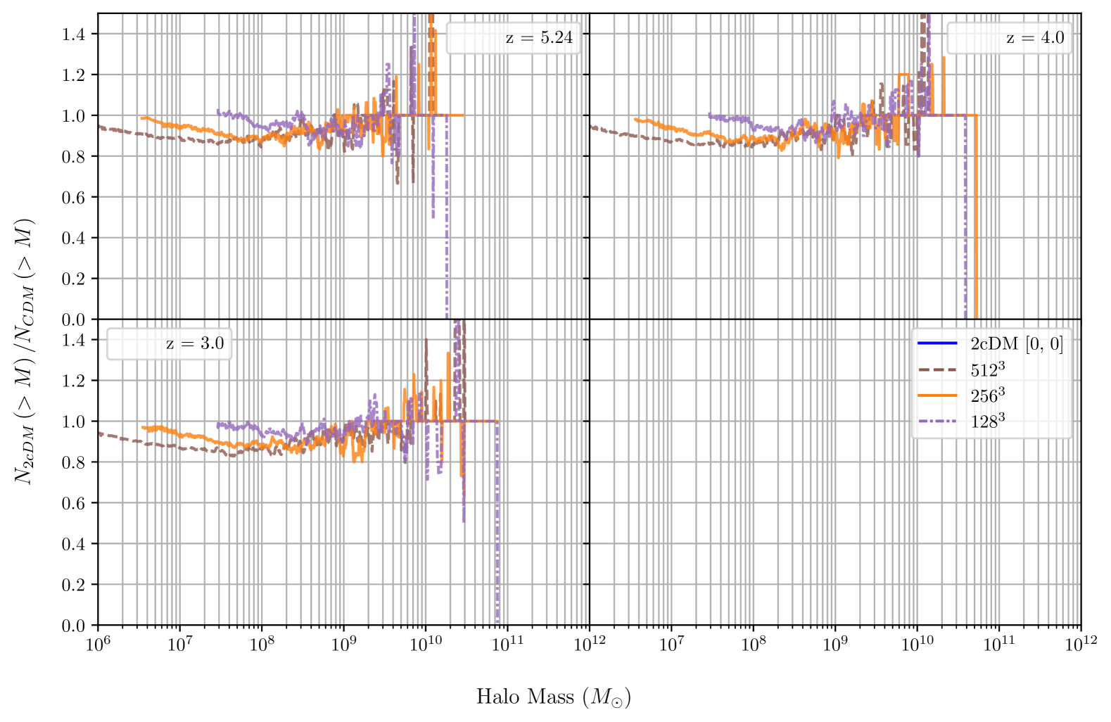
Figure 20: (Right) Comparing the halo mass function across simulations with varying $N_{part}$. Blue lines represent 2cDM simulations, while red lines represent CDM simulations. Solid lines correspond to the fiducial particle number of $256^{3}$. Dash-dotted and dashed lines correspond to particle numbers of $128^{3}$ and $512^{3}$ respectively. All simulations presented here are hydrodynamic. (Left) The ratio between 2cDM and CDM halo mass functions. Lines are coloured by box size.

Figure 21: The $V_{max}$ functions for the $N_{part}$ scaling test. colouring is identical to Figure 20.

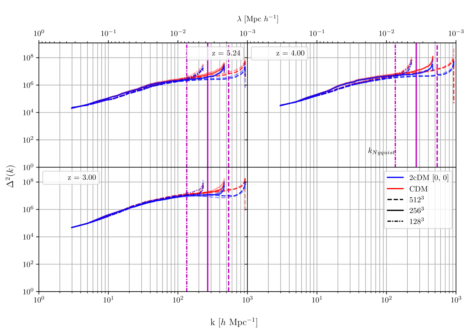
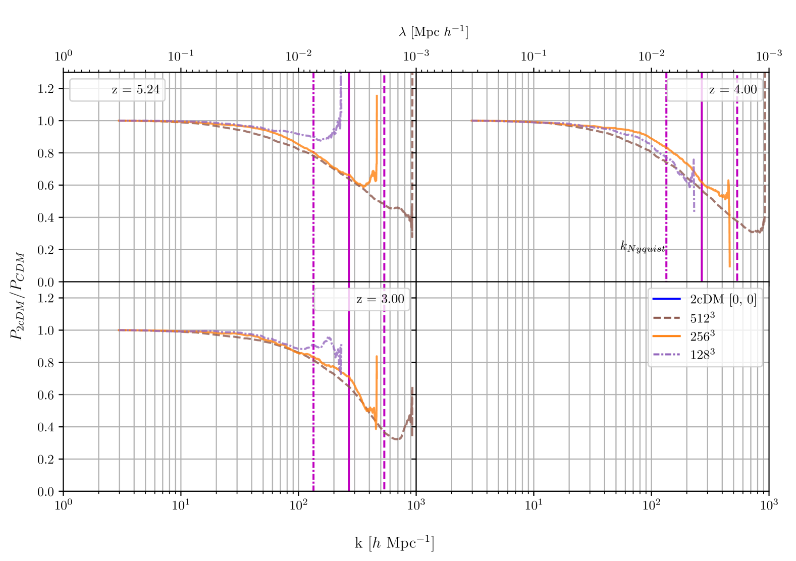
Figure 22: The dimensionless power spectra for the $N_{part}$ scaling test. Vertical lines denote the Nyquist wavenumber for the simulations. colouring is identical to Figure 20. Higher particle number leads to better resolved small structure. The trend in the suppression that we see at lower resolutions continues well at higher resolutions.

Figure 23: The ratio between power spectra for hydrodynamic and $N$-body simulations for the the $N_{part}$ scaling test. We note that the enhancement seen in the power spectra lie within the error bounds of our fiducial simulations. Lower gas particle numbers lead to worse convergence, suggesting a minimum particle number for producing the correct baryonic effects.

References

- An et al. (2024) An R., Nadler E. O., Benson A., Gluscevic V., 2024, arXiv e-prints, p. arXiv:2411.03431
- Bell et al. (2022) Bell N. F., Dent J. B., Dutta B., Kumar J., Newstead J. L., 2022, arXiv e-prints, p. arXiv:2208.08020
- Bertuzzo et al. (2022) Bertuzzo E., Scaffidi A., Taoso M., 2022, Journal of High Energy Physics, 2022, 100
- Bird (2017) Bird S., 2017, GenPK: Power spectrum generator, Astrophysics Source Code Library, record ascl:1706.006
- Boylan-Kolchin et al. (2011a) Boylan-Kolchin M., Bullock J. S., Kaplinghat M., 2011a, MNRAS, 415, L40
- Boylan-Kolchin et al. (2011b) Boylan-Kolchin M., Bullock J. S., Kaplinghat M., 2011b, MNRAS, 415, L40
- Chisari et al. (2019) Chisari N. E., et al., 2019, The Open Journal of Astrophysics, 2, 4
- Creasey et al. (2017) Creasey P., Sameie O., Sales L. V., Yu H.-B., Vogelsberger M., Zavala J., 2017, MNRAS, 468, 2283
- Croft et al. (1998) Croft R. A. C., Weinberg D. H., Katz N., Hernquist L., 1998, ApJ, 495, 44
- Cyr-Racine et al. (2016) Cyr-Racine F.-Y., Sigurdson K., Zavala J., Bringmann T., Vogelsberger M., Pfrommer C., 2016, Phys. Rev. D, 93, 123527
- Dienes et al. (2022) Dienes K. R., Huang F., Kost J., Thomas B., Yu H.-B., 2022, Phys. Rev. D, 106, 123521
- Dolag et al. (2009) Dolag K., Borgani S., Murante G., Springel V., 2009, MNRAS, 399, 497
- Duerr et al. (2021) Duerr M., Ferber T., Garcia-Cely C., Hearty C., Schmidt-Hoberg K., 2021, Journal of High Energy Physics, 2021, 146
- Emken et al. (2022) Emken T., Frerick J., Heeba S., Kahlhoefer F., 2022, Phys. Rev. D, 105, 055023
- Flores & Primack (1994) Flores R. A., Primack J. R., 1994, ApJ, 427, L1
- Fry et al. (2015) Fry A. B., et al., 2015, MNRAS, 452, 1468
- Garrison-Kimmel et al. (2014) Garrison-Kimmel S., Boylan-Kolchin M., Bullock J. S., Kirby E. N., 2014, MNRAS, 444, 222
- Gebhardt et al. (2024) Gebhardt M., et al., 2024, MNRAS, 529, 4896
- Harris et al. (2020) Harris C. R., et al., 2020, Nature, 585, 357
- Hui & Gnedin (1997) Hui L., Gnedin N. Y., 1997, MNRAS, 292, 27
- Hunter (2007) Hunter J. D., 2007, Computing in Science & Engineering, 9, 90
- Iršič et al. (2024) Iršič V., et al., 2024, Phys. Rev. D, 109, 043511
- Kamada et al. (2017) Kamada A., Kaplinghat M., Pace A. B., Yu H.-B., 2017, Phys. Rev. Lett., 119, 111102
- Kamada et al. (2022) Kamada A., Kim H. J., Park J.-C., Shin S., 2022, J. Cosmology Astropart. Phys., 2022, 052
- Kim et al. (2018) Kim S. Y., Peter A. H. G., Hargis J. R., 2018, Phys. Rev. Lett., 121, 211302
- Kim et al. (2023) Kim J. H., Kong K., Lim S. H., Park J.-C., 2023, arXiv e-prints, p. arXiv:2312.07660
- Kim et al. (2024) Kim J. H., Kong K., Lim S. H., Park J.-C., 2024, arXiv e-prints, p. arXiv:2410.05382
- Klypin et al. (1999) Klypin A., Kravtsov A. V., Valenzuela O., Prada F., 1999, ApJ, 522, 82
- Klypin et al. (2001) Klypin A., Kravtsov A. V., Bullock J. S., Primack J. R., 2001, ApJ, 554, 903
- Kohm et al. (2024) Kohm J., Sanderson R., Hey D., Huber D., 2024, in American Astronomical Society Meeting Abstracts. p. 107.06
- Kong et al. (2015) Kong K., Mohlabeng G., Park J.-C., 2015, Physics Letters B, 743, 256
- Medvedev (2000) Medvedev M. V., 2000, arXiv e-prints, pp astro–ph/0010616
- Medvedev (2001) Medvedev M., 2001, arXiv e-prints, pp astro–ph/0105156
- Medvedev (2010a) Medvedev M. V., 2010a, arXiv e-prints, p. arXiv:1004.3377
- Medvedev (2010b) Medvedev M. V., 2010b, Journal of Physics A Mathematical General, 43, 372002
- Medvedev (2014a) Medvedev M. V., 2014a, Phys. Rev. Lett., 113, 071303
- Medvedev (2014b) Medvedev M. V., 2014b, J. Cosmology Astropart. Phys., 2014, 063
- Moore et al. (1999) Moore B., Ghigna S., Governato F., Lake G., Quinn T., Stadel J., Tozzi P., 1999, ApJ, 524, L19
- Myrtaj et al. (2022) Myrtaj O., Sameie O., Boylan-Kolchin M., 2022, in American Astronomical Society Meeting #240. p. 334.04D
- Navarro et al. (1996) Navarro J. F., Frenk C. S., White S. D. M., 1996, ApJ, 462, 563
- Navarro et al. (1997) Navarro J. F., Frenk C. S., White S. D. M., 1997, ApJ, 490, 493
- O’Neil et al. (2022) O’Neil S., et al., 2022, arXiv e-prints, p. arXiv:2210.16328
- Oman et al. (2015) Oman K. A., et al., 2015, MNRAS, 452, 3650
- Pillepich et al. (2018) Pillepich A., et al., 2018, MNRAS, 473, 4077
- Planck Collaboration et al. (2016) Planck Collaboration et al., 2016, A&A, 594, A13
- Rose et al. (2023) Rose J. C., Torrey P., Vogelsberger M., O’Neil S., 2023, MNRAS, 519, 5623
- Rose et al. (2024) Rose J. C., et al., 2024, arXiv e-prints, p. arXiv:2405.00766
- Roy et al. (2023) Roy S., Shen X., Lisanti M., Curtin D., Murray N., Hopkins P. F., 2023, ApJ, 954, L40
- Roy et al. (2024) Roy S., Shen X., Barron J., Lisanti M., Curtin D., Murray N., Hopkins P. F., 2024, arXiv e-prints, p. arXiv:2408.15317
- Sales et al. (2022) Sales L. V., Wetzel A., Fattahi A., 2022, Nature Astronomy, 6, 897
- Sameie et al. (2021) Sameie O., et al., 2021, MNRAS, 507, 720
- Schneider et al. (2019) Schneider A., Teyssier R., Stadel J., Chisari N. E., Le Brun A. M. C., Amara A., Refregier A., 2019, J. Cosmology Astropart. Phys., 2019, 020
- Schutz & Slatyer (2015) Schutz K., Slatyer T. R., 2015, J. Cosmology Astropart. Phys., 2015, 021
- Spergel & Steinhardt (2000) Spergel D. N., Steinhardt P. J., 2000, Phys. Rev. Lett., 84, 3760
- Springel (2005) Springel V., 2005, MNRAS, 364, 1105
- Springel et al. (2001) Springel V., White S. D. M., Tormen G., Kauffmann G., 2001, MNRAS, 328, 726
- Springel et al. (2008) Springel V., et al., 2008, MNRAS, 391, 1685
- Straight et al. (2025) Straight M. C., et al., 2025, arXiv e-prints, p. arXiv:2501.16602
- Todoroki & Medvedev (2019a) Todoroki K., Medvedev M. V., 2019a, MNRAS, 483, 3983
- Todoroki & Medvedev (2019b) Todoroki K., Medvedev M. V., 2019b, MNRAS, 483, 4004
- Todoroki & Medvedev (2022) Todoroki K., Medvedev M. V., 2022, MNRAS, 510, 4249
- Torrey et al. (2014) Torrey P., Vogelsberger M., Genel S., Sijacki D., Springel V., Hernquist L., 2014, MNRAS, 438, 1985
- Tulin & Yu (2018) Tulin S., Yu H.-B., 2018, Phys. Rep., 730, 1
- Van Rossum & Drake (2009) Van Rossum G., Drake F. L., 2009, Python 3 Reference Manual. CreateSpace, Scotts Valley, CA
- Vargya et al. (2022) Vargya D., Sanderson R., Sameie O., Boylan-Kolchin M., Hopkins P. F., Wetzel A., Graus A., 2022, MNRAS, 516, 2389
- Viel et al. (2013) Viel M., Becker G. D., Bolton J. S., Haehnelt M. G., 2013, Phys. Rev. D, 88, 043502
- Villaescusa-Navarro et al. (2021) Villaescusa-Navarro F., et al., 2021, ApJ, 915, 71
- Virtanen et al. (2020) Virtanen P., et al., 2020, Nature Methods, 17, 261
- Vogelsberger et al. (2012a) Vogelsberger M., Zavala J., Loeb A., 2012a, MNRAS, 423, 3740
- Vogelsberger et al. (2012b) Vogelsberger M., Sijacki D., Kereš D., Springel V., Hernquist L., 2012b, MNRAS, 425, 3024
- Vogelsberger et al. (2014a) Vogelsberger M., et al., 2014a, MNRAS, 444, 1518
- Vogelsberger et al. (2014b) Vogelsberger M., Zavala J., Simpson C., Jenkins A., 2014b, MNRAS, 444, 3684
- Vogelsberger et al. (2016) Vogelsberger M., Zavala J., Cyr-Racine F.-Y., Pfrommer C., Bringmann T., Sigurdson K., 2016, MNRAS, 460, 1399
- Vogelsberger et al. (2019) Vogelsberger M., Zavala J., Schutz K., Slatyer T. R., 2019, MNRAS, 484, 5437
- Wang et al. (2013) Wang M.-Y., Croft R. A. C., Peter A. H. G., Zentner A. R., Purcell C. W., 2013, Phys. Rev. D, 88, 123515
- van Daalen et al. (2011) van Daalen M. P., Schaye J., Booth C. M., Dalla Vecchia C., 2011, MNRAS, 415, 3649
- van Daalen et al. (2020) van Daalen M. P., McCarthy I. G., Schaye J., 2020, MNRAS, 491, 2424