On spectral scaling laws for averaged turbulence on the sphere
Abstract.
Spectral analysis for a class of Lagrangian-averaged Navier–Stokes (LANS) equations on the sphere is carried out. The equations arise from the Navier–Stokes equations by applying a Helmholtz filter of width to the advecting velocity times. Power laws for the energy spectrum are derived and indicate a -dependent scaling at wave numbers with . The energy and enstrophy transfer rates distinctly depend on the averaging, allowing control over the energy flux and the enstrophy flux separately through the choice of averaging operator. A necessary condition on the averaging operator is derived for the existence of the inverse cascade in two-dimensional turbulence. Numerical experiments with a structure-preserving integrator confirm the expected energy spectrum scalings and the robustness of the double cascade under choices of the averaging operator.
1. Introduction
The distribution of energy over a vast range of scales of motion is a characteristic feature of turbulent flows. Consequently, fully scale-resolving numerical simulations of turbulence are computationally unfeasible. This has prompted the development of simulation strategies that deal with modified systems of partial differential equations with reduced dynamical complexity. Among these is a geometric regularization principle for ideal fluids as proposed by Holm, Marsden, and Ratiu [21], referred to as -modeling. It alters the nonlinear advection terms and thereby gives rise to regularized Euler equations. Adding a viscous term then leads to the Navier–Stokes- (NS-, also referred to as Lagrangian-averaged NS- or LANS-) model, in which the energy content of small scales is suppressed [28].
In this work, we study the two-dimensional NS- model on the sphere and extend the model to a larger class of averaging operators, which we refer to as the --Navier–Stokes (--NS) equations. More specifically, the contributions are the following.
-
(1)
We perform spectral analysis for averaged turbulence on the sphere to obtain scaling laws for the double cascade, using the geometric stream function-vorticity formulation. The analysis is carried out for the --NS equations, which encompass both the standard NS equations and the NS- model. By adhering to the stream function-vorticity formulation, we exploit geometric properties of the two-dimensional Euler equations and simplify previous work on the scaling of the Navier–Stokes equations [26]. Specifically, without averaging we recover the double cascade of two-dimensional turbulence. When averaging, a steep energy scaling is found at high wave numbers, where the onset to this scaling is determined by and the scaling rate is determined by the averaging strength .
-
(2)
A necessary condition is derived for the inverse energy cascade to exist in averaged turbulence, which imposes certain conditions on the averaging operator. This ensures that the analysis is valid for any type of operator relating the vorticity and stream function that decays sufficiently fast for high wave numbers.
-
(3)
The energy and enstrophy flux rates are derived and are shown to distinctly depend on the chosen averaging operator. The disparity between these flux rates permits control over the fluxes through an appropriate choice of averaging operator.
-
(4)
The derived energy scaling laws are supported by numerical results carried out with a structure-preserving integrator, providing robust numerical support of the theoretically derived double cascade in averaged turbulence.
The averaged Navier–Stokes equations are a model for the dynamics of the large-scale flow in a turbulent fluid. Here, the spatial domain is the two-dimensional sphere and the governing equations are given by
| (1) |
where denotes time derivative, and denote the covariant derivative and its transpose under the -metric, denotes the averaged velocity field of the fluid, and is the velocity, or momentum. The parameter determines the viscosity of the fluid, is the friction parameter, and is a length scale associated with the smoothing effect of the Helmholtz operator. The parameter determines the strength of the averaging, or, for integer values, the number of times the Helmholtz filter is applied. The addition of marks an extension of the averaging operator when compared to preceding studies of the -model. We refer to equation 1 as the - averaged Navier–Stokes equations.
An equivalent formulation of equation 1 is the stream function-vorticity formulation. We distinguish between the velocity and the momentum via the relations and , where is the skew-gradient on the sphere, obtained by rotating the gradient by in the tangent plane of the sphere. The scalar functions and are referred to as the vorticity and the stream function, respectively. The formulation via and avoids having to deal with the covariant derivative terms in (1), which can be cumbersome numerically, and which simplifies the spectral analysis of energy fluxes. The resulting formulation reads
| (2) |
where is the vorticity of the fluid, and is the stream function, which is determined up to a constant. The Poisson bracket is defined by
| (3) |
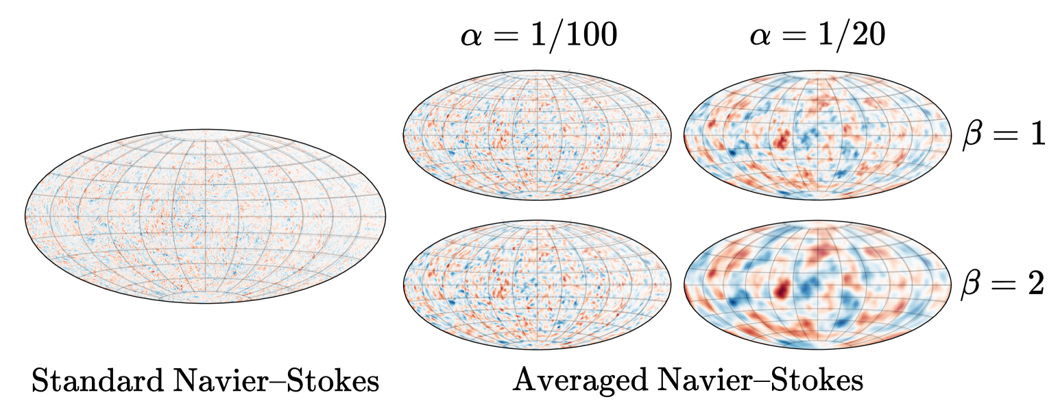
and its unaltered appearance in (2) alludes to the geometric properties of -modelling [21]. The --averaged Navier–Stokes equations (2) are a generalization of the usual Navier–Stokes equations, which are obtained as . A qualitative illustration of the averaging is given in figure 1, depicting the smoothed vorticity fields for several values of and .
There are several possible notions of energy and enstrophy in the averaged Navier–Stokes equations. However, a natural choice is to consider the energy and enstrophy that are preserved in the limit of vanishing viscosity and friction. This energy is given by
| (4) |
and the enstrophy is given by
| (5) |
In fact, the --averaged Euler equations, given by
| (6) |
form a Hamiltonian system on with Hamiltonian . The smoothed stream function enters the definition of the energy, thereby inhibiting the creation of scales below a certain threshold defined by and yielding a nonlinear dispersive modification of the Navier–Stokes equations [12].
For the -model, the parameter profoundly affects the distribution of energy across the resolvable scales of motion [29]. The energy scalings in spectral space of the --averaged Navier–Stokes equations are the focus of the current study. In three dimensions, the energy spectrum of the NS- model shows a scaling at wave numbers where the averaging is dominant, rather than the standard scaling [12]. A similar result has been established for the two-dimensional NS- model theoretically and numerically, yielding a scaling in the direct enstrophy cascade regime at wave numbers where the averaging is strong [28]. Furthermore, the latter showed that the cascading conserved quantity in the -model determines the scaling of derived statistical quantities in two-dimensional turbulence.
The suppression of small-scale motions in averaged turbulence is computationally appealing, since this property facilitates numerical simulations. This property has been exploited in computational large-eddy simulation (LES) studies. Re-writing the averaged equations of motion in terms of the smoothed momentum casts them into a standard LES template, where the divergence of the turbulent stress tensor is modeled as a forcing term [13]. The nonlinearly dispersive -model, as opposed to commonly used dissipative models, encompasses Leray regularization [25, 15] and has shown favorable results for turbulent mixing when compared to eddy-viscosity models [13, 14]. The -modelling approach has also found meaningful applications in ocean modelling, where transport phenomena often play an important role. The -model and Leray model are studied in the context of the primitive equation ocean model [17, 18], yielding flow statistics resembling those obtained with no-model high-resolution simulations. In addition, qualitative flow dynamics also complied with higher-resolution numerical simulations. The present focus is the distribution of energy in two-dimensional homogeneous isotropic turbulence on the sphere, which is studied in the context of the --Navier–Stokes equations. The novel inclusion of describes the rate at which high-frequency flow components are curbed, and thereby enables stricter control over the roll-off of the energy spectrum. Furthermore, a range of numerical experiments are carried out to study the robustness of the --model and investigate at which parameter regimes the large-scale flow features can still be predicted reliably.
The Lagrangian-averaged Navier–Stokes equations share mathematical and statistical properties with the standard Navier–Stokes equations. For example, the -Navier–Stokes equations can be cast in a variational formulation [31], using the assumption that fluctuations smaller than length scale are frozen in the mean flow. In three-dimensional turbulence, the -model is shown to not affect the connection between second- and third-order structure functions at separation distances larger than [19], further substantiating that the model is suited to accurately resolve the large scales of turbulent motion. Moreover, a derivation of the NS- equations from the Kelvin circulation theorem is given by taking the integral over a loop moving with a spatially filtered velocity [12]. For two-dimensional fluids, this implies that inviscid averaged equations retain the conserved quantities of the two-dimensional Euler equations. The --NS model may thus serve as a deterministic reference model for flow descriptions in which the transport velocity is stochastically perturbed, such as (Lagrangian-averaged) stochastic advection by Lie transport ((LA-)SALT) [1, 20, 10].
In this paper, we make theoretical predictions about the transfer and cascade of energy and enstrophy in the --NS equations on the sphere, and we verify these predictions numerically using Zeitlin’s structure-preserving spatial discretization of the Euler equations [35, 36]. This computational method replaces the Hamiltonian system on the Poisson algebra of smooth zero-mean functions on the sphere with a Hamiltonian system on the Lie algebra of skew-Hermitian matrices of size . In particular, as the mathematical structure of the continuous system and the discrete system are geometrically and algebraically similar, we expect that the spectral behavior of the continuous system is accurately captured by the discrete system even at modest resolutions. This has been demonstrated for homogeneous isotropic turbulence on the sphere, where Kraichnan’s double cascade [24] is accurately captured in Zeitlin-based numerical simulations [8].
The paper is structured as follows. In section 2 we apply the analysis of Lindborg and Nordmark [26] to derive the cascade directions and spectrum scaling rates for averaged turbulence. This is followed by numerical experiments in section 3. We verify the results of section 2 in two experiments, to study the averaging effect on both cascades. The paper is concluded in section 4.
2. Cascade directions and spectrum scalings
In this section, we provide arguments for the transfer and cascade of energy and enstrophy for the --averaged Navier–Stokes equations (2).
We show that the double cascade of two-dimensional turbulence also holds for the averaged equations. That is, energy and enstrophy below a forcing wave number move from low to high wave numbers, and in the opposite direction above the forcing wave number, as predicted by Kraichnan [24]. Briefly, this is because the definitions of the energy, enstrophy and the corresponding rates of change in the NS- model (2) equals the spherical two-dimensional case up to a dimensionless wave number-dependent factor, since the averaging operator is diagonalized by the spherical harmonics basis. The key is to identify in which expressions this scaling factor appears, and how it affects the energy and enstrophy transfer rates.
We derive these expressions in detail by expanding the relevant physical quantities in the spherical harmonic basis, following the approach of Lindborg and Nordmark [26]. To this end, let be the spherical harmonic functions, i.e., the eigenfunctions of the Laplace–Beltrami operator . The corresponding eigenvalues are given by
| (7) |
Consequently, a real scalar function can be expanded as
| (8) |
where with . Since the stream function has the expansion
| (9) |
it follows from the relation that
| (10) |
or, in other words, that . Consequently, the energy is expressed as
We set to be the energy in mode . Furthermore, is a natural definition of the energy since it
-
(1)
is the Hamiltonian of the - Euler equations;
-
(2)
is a conserved quantity in the case of vanishing viscosity and friction.
In the limit of vanishing viscosity and friction, there are an infinite number of conserved quantities called Casimirs, given by integrals of analytic functions of the vorticity. All Casimirs can thus be expanded in Casimir functions of the form , where . A well-known Casimir is the enstrophy, given by
Here, we use the series expansion (10) to obtain the right-hand side. The enstrophy in mode is given by
With these definitions at hand, we turn our attention to the corresponding rates of change. Equation 2 induces an evolution of , which is found by multiplying (2) by and integrating over ,
| (11) |
Note that we also have
We follow Lindborg and Nordmark [26] and introduce the quantity
| (12) |
so that the nonlinear term in (11) is given by
| (13) |
Equation 12 reveals that the behavior of is intimately connected to the Lie algebra structure of the Poisson bracket (3), and that the triadic interactions, central in the analysis of Kraichnan [24], Fjørtoft [11] and Lindborg and Nordmark [26]m are captured by the structure constants of the Poisson algebra in the spherical harmonics basis. The geometric analysis of the triadic interactions warrants its own study and is not further investigated here.
The remaining terms in (11) are rewritten as
| (14) | ||||
| (15) |
where we have used that . Thus, the energy transfer equation for the --averaged Navier–Stokes equations reads
| (16) |
Note that this is the same equation as for the (standard) Navier–Stokes equations. To continue the analysis, we need to study . Observe that and may be expanded into their respective modes, so that is rewritten as
| (17) |
By noting that , and all consist of finite linear combinations of spherical harmonics, it becomes evident from (17) that the qualitative behavior of is described by the structure constants . In particular, this is independent of the values of and . Consequently, the analysis of the energy transfer in the --averaged Navier–Stokes equations is identical to the analysis of the usual Navier–Stokes equations on the sphere, detailed by Lindborg and Nordmark [26], up to the scaling factor .
We now show that the kinetic energy dissipation vanishes for the averaged Navier–Stokes equations in the limit of small viscosity, following the same analysis as Lindborg and Nordmark [26]. This result implies that there can be no Richardson energy cascade, and that energy is instead transferred to large scales in an inverse cascade. The evolution of the average total energy and enstrophy are given by
| (18) | |||
| (19) |
where and respectively denote the average energy and enstrophy dissipation rates.
By omitting energy and enstrophy loss due to friction, i.e., terms with , the result of Lindborg and Nordmark [26] can be cast in the present notation as
| (20) | |||
| (21) |
We deduce that kinetic energy dissipation vanishes in the limit . Indeed, inserting into the equation of yields
| (22) |
Since
| (23) |
for all , we have that
| (24) |
The enstrophy is a positive quantity that is non-increasing in time, since is nonnegative. This indicates that the kinetic energy dissipation has an upper bound in terms of the viscosity and the total enstrophy. The enstrophy is bounded from above; hence the energy dissipation must vanish if . (It is clear that the kinetic energy dissipation cannot be negative.) This result does not follow in three-dimensional turbulence, where the enstrophy can grow due to vortex stretching [4].
We continue the analysis by studying the spectral energy and enstrophy fluxes. These are respectively defined as
| (25) | |||
| (26) |
where energy and enstrophy conservation is used to obtain the right-hand sides [26]. Now, the analysis of the fluxes presented by Lindborg and Nordmark [26] can be repeated verbatim since the behavior of the fluxes is determined by the structure constants, which are independent of and . The only difference is that the scaling factor describing the enstrophy transfer within a triad of modes, when given in terms of the energy transfer within these modes, is given by instead of . Thus, the qualitative reasoning in Lindborg and Nordmark [26, Section 5-6] can still be applied. We therefore have that the enstrophy flux is positive when the energy flux is zero, and vice versa for the energy flux. Moreover, in the case of narrow-band forcing in spectral space, more energy is transferred to low wave numbers than to high wave numbers, and the opposite holds true for the enstrophy [16].
Assume now that the forcing is concentrated at a wave number , such that . In that case, we expect three distinct scaling regimes to appear in the energy spectrum. At wave numbers , i.e., wave numbers at which the effect of the averaging is negligible, the distribution of energy should follow the double cascade observed in the standard Navier–Stokes equations. That is, the energy spectrum scales as in the energy cascade range (when ) and as in the enstrophy cascade range (when ). This means that the large flow scales are largely unaffected by the averaging. A third regime appears at wave numbers such that , i.e., wave numbers at which the effect of the averaging is significant. In this regime, dimensional analysis as in Kraichnan [24] and the approximation for large wave numbers, as in Lindborg and Nordmark [26], predicts that
| (27) |
Equivalently, this implies that the energy spectrum scales as
| (28) |
resulting in a steeper decline of the energy than predicted in the enstrophy cascade range, with a stronger suppression of energy as increases. This is in line with Lunasin et al. [28], who derive via dimensional analysis and numerical simulations that the energy spectrum should scale as for .
Remark 2.1.
Note that the above derivation is not limited to the operator . Indeed, let . If is a linear operator defined by
for some function such that
-
(1)
is a dimensionless quantity,
-
(2)
,
then the above analysis also holds when . For instance, could be chosen such that it equals if is small, and only apply - smoothing for wave numbers above a specified value.
3. Numerical experiments
We now move on to numerical demonstrations of the results derived in section 2.
3.1. Computational method
The spatial discretization of the equations of motion (2) follows the self-consistent finite-dimensional truncation method of Zeitlin [36]. In the absence of viscous dissipation and external forcing, the vorticity equation (2) forms a Lie–Poisson system [2, 30] on the space of smooth functions on the sphere . The Zeitlin approach provides a finite-dimensional truncation of the Poisson bracket through geometric quantization [22, 5, 6], thereby enabling a fully structure-preserving discretization of the convection operator. The method relies on a projection of smooth functions to complex skew-Hermitian matrices and replacing the Poisson bracket by the matrix commutator for . A spherical harmonic basis element is then identified with a matrix basis . The value can be thought of as the adopted numerical resolution, and we have for :
-
(1)
,
-
(2)
,
-
(3)
,
where denotes the spectral norm. The Laplacian operator is replaced by the discrete Laplacian operator of Hoppe and Yau [23]. The critical property of is that the basis elements are the eigenvectors with corresponding eigenvalues , analogous to the Laplacian and the spherical harmonics.
A discrete approximation of the vorticity is obtained after identifying a spherical harmonic function with the matrix harmonic . The spherical harmonic coefficients of the vorticity are computed as , after which the matrix approximation of reads
| (29) |
The stream matrix is computed analogously from . The discrete approximation to the equations of motion (2) are given by
| (30) |
In particular, the system (30) has Casimir functions in the absence of viscosity and external forcing and damping. These are defined as the traces of the powers of vorticity [35],
| (31) |
analogous to the integrated powers of vorticity in the original system. We employ an isospectral Lie–Poisson integrator [33, 32, 7] for the convective term to preserve these Casimir functions. The viscous dissipation and external forcing and damping terms are integrated using a Crank–Nicolson scheme [9]. We denote these time integration schemes over a time interval of length by and , respectively. A single time integration step of length for (30) is then carried out using the Strang splitting [34] as
| (32) |
where the superscript denotes the time step. This provides a second-order time discretization of the dynamics.
3.2. Details of the numerical experiments
Two series of numerical experiments are carried out at resolution . All results are compared to numerical results of the standard Navier–Stokes equations obtained with the same computational method. Each numerical realization is driven to a statistically stationary state via an external forcing placed at a forcing wave number , combined with a friction coefficient to prevent energy build-up in low wave number modes. A single Reynolds number is chosen for both sets of simulations, where we adopt the forcing-dependent definition as presented by Kraichnan [24]. The external forcing is defined as white noise in time to control the energy injection rate [3], multiplied by a magnitude . We estimate as and adjust the viscosity parameter so that a specified Reynolds number is obtained. All numerical simulations are run until a statistically stationary state is reached, which we define by having a constant time-averaged energy spectrum over different time intervals.
In the first set of experiments, the forcing is placed at wave number to allow the maximal possible development of the enstrophy inertial subrange. The Reynolds number is set to 1200. A sequence of values for and is applied in separate numerical simulations to obtain clear numerical evidence of the different scaling regimes predicted in the previous section. Here, we adopt all combinations of and .
The second set consists of simulations in which a double cascade can develop, by placing the external forcing at wave number and setting the Reynolds number at 600. We demonstrate that this choice of forcing already allows for the formation of a double cascade at the employed resolution. The same values of and are applied as in the first set of experiments to study the effects of the averaging procedure in both regimes of the classical double cascade.
3.3. Enstrophy cascade scalings
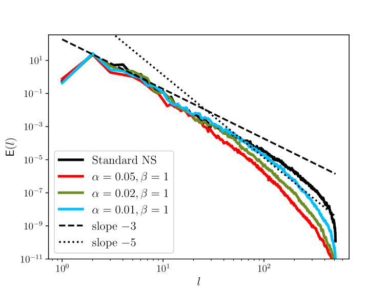
The first set of numerical simulations is used to verify the predicted scaling laws in the enstrophy cascade regime for different values of and . The energy spectra are shown in figure 2 along with reference scalings. The standard Navier–Stokes result is the same in both panels, and the departures from this energy spectrum clearly display the effect of the averaging on the distribution of energy across the scales of motion.
The left panel shows the results for . The predicted scaling is attained in the results of the averaged Navier–Stokes equations. This is best observed for , which causes the averaging term to become dominant at wave numbers well separated from wave numbers at which dissipative effects are strong. The averaging is further amplified for , visible from the energy spectra in the right panel. A clear scaling is found for these parameter values, which agrees with the prediction in the previous section. The cusp between the two scalings in the energy spectrum appears sharper than for , which is due to the term growing exponentially for increasing and thus strongly increasing the averaging effect.
3.4. Robustness of the double cascade and spectral fluxes
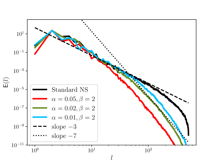
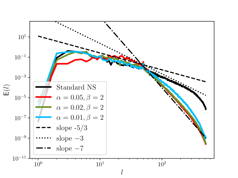
In the second set of numerical simulations, we investigate how the averaging affects the double cascade observed in two-dimensional turbulence. The corresponding energy spectra are given in figure 3, where the spectrum of the standard Navier–Stokes equations is the same in both panels for comparison. Even at the modest adopted resolution , the and scalings as predicted by Kraichnan are accurately captured. The --averaged Navier–Stokes equations display the expected scalings at high wave numbers for all considered values of and . This coincides with the results reported in the previous subsection. Of particular interest are the results obtained with (), where the term becomes significant at wave numbers smaller than the forcing wave number . For this value of , the averaging effect for is difficult to discern at wave numbers . However, a deviation is observed in the inverse energy cascade for and .
Injecting the energy at wave number allows for a clear identification of the energy and enstrophy fluxes. The energy is expected to move from the forcing wave number towards low wave numbers in the standard Navier–Stokes equations [24, 26], whereas the enstrophy is expected to move to high wave numbers. This qualitative behavior is not expected to change for the --Navier–Stokes equations, following the analysis in section 2. To demonstrate this, we take a vorticity field from the standard Navier–Stokes equations in a statistically stationary state and compute the corresponding stream function for various values of and . Subsequently, the spectral fluxes are computed following their respective definitions in (25) and (26).
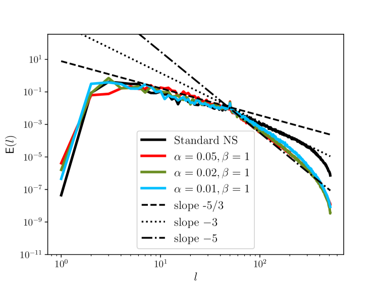
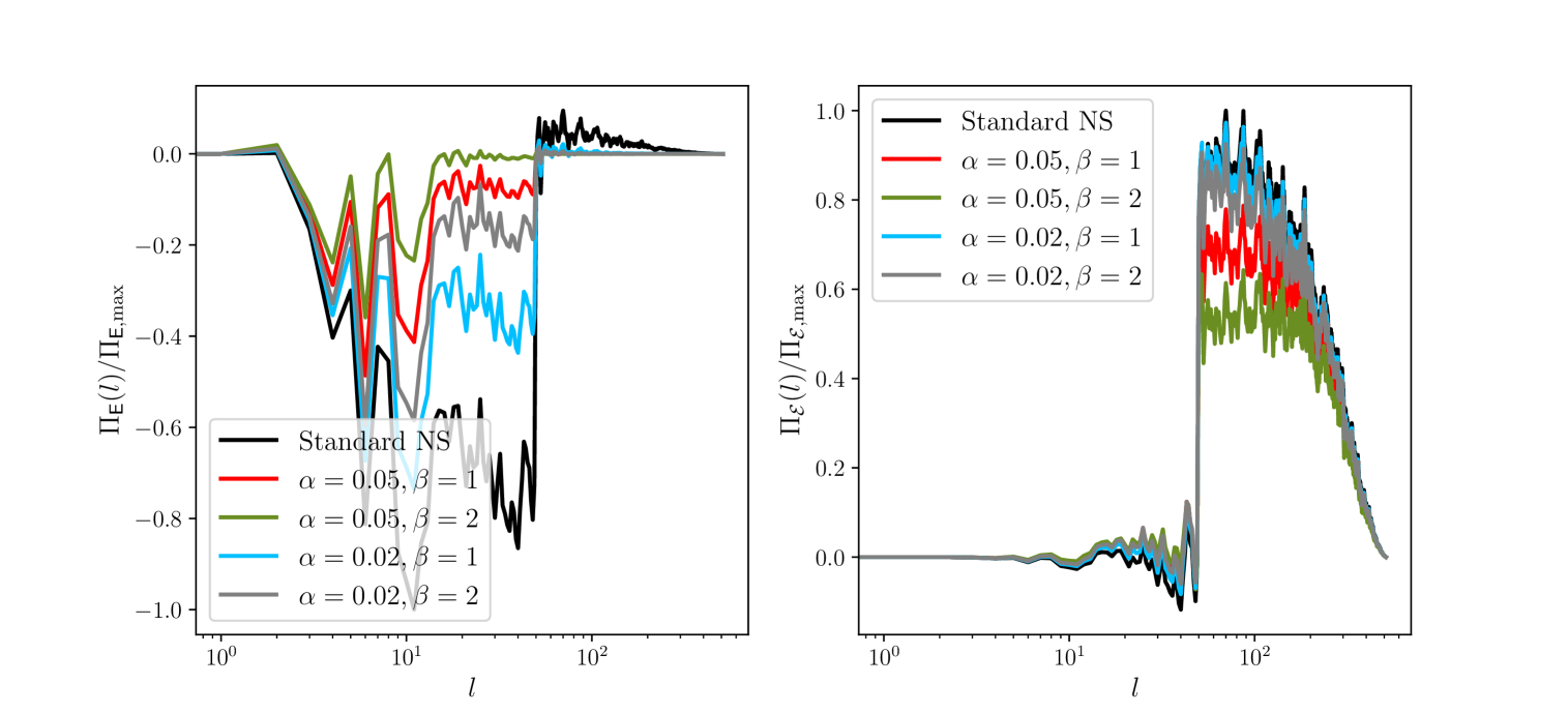
The fluxes are presented in figure 4, normalized by the maximum absolute value of the corresponding flux for the standard Navier–Stokes equations. The forcing causes the jump observed in both fluxes at . The negative energy flux for indicates energy moving to low wave numbers. Similarly, the positive enstrophy flux for implies that enstrophy is transferred to high wave numbers. This qualitative behavior is also observed in the fluxes of the --Navier–Stokes equations, suggesting that the double cascade is still present in the averaged equations. After all, the transfer function does not change qualitatively since it is defined in terms of the Poisson bracket and the vorticity, which both do not change when averaging, and the stream function, which is suppressed at higher wave numbers. This smoothing effect is especially visible as the energy fluxes approach zero at wave numbers for and . A less pronounced damping is visible in the enstrophy flux. The disparity between the damping of the energy flux and the enstrophy flux is readily explained by the appearance of the stream function in their respective definitions. Namely, the stream function is subject to the averaging operator, which dampens the component at wave number by a factor . This factor appears twice in the definition of the energy flux and only once in the enstrophy flux. Thus, the smoothing has a larger effect on the former than on the latter. The different effects on each of these fluxes implies that one can control the relation of the fluxes through an appropriate choice of averaging operator.
4. Conclusions
In this paper, we carried out spectral analysis for averaged turbulence on the sphere. The scaling laws for a class of Lagrangian-averaged Navier–Stokes equations were derived by extending the results of Lindborg and Nordmark [26] and utilizing the geometry of two-dimensional fluids in two distinct ways. First, the scaling laws were determined by studying the governing equations in stream function-vorticity formulation that yielded simple expressions for the relevant terms. Second, the averaging operator was applied in a manner that retains the underlying geometric structure of the equations, thereby enabling an extension of previous results to encompass Lagrangian-averaged turbulence.
The averaging operator was found to suppress the energy in high wave number flow components, which is in agreement with previous studies on the Navier–Stokes- model. Here, an extension to previous models was included through an additional parameter that determines the number of times that the smoothing is applied. This lead to a class of averaging operators that not only determines the onset of the energy suppression, but also allows for control over the rate of suppression. In particular, a necessary condition for the existence of the inverse cascade in two-dimensional turbulence was derived for the averaging operator. Furthermore, the energy flux and enstrophy flux were found to have a distinct dependence on the parameters of the averaging operator, allowing for control over these fluxes through the choice of parameters. The derived scaling laws, existence of the inverse cascade, and the energy and enstrophy fluxes were demonstrated in numerical experiments performed with a structure-preserving integrator for flows on the sphere.
The results presented in this paper can serve as a reference for spectral analysis of other global geophysical fluid models that possess similar geometric properties as the Euler equations, such as the quasi-geostrophic equations [27]. Additionally, the current results can be compared to geophysical fluid models where the advection velocity is stochastically perturbed and a smoothing effect can be achieved by taking the expectation [1, 20, 10].
References
- [1] M. Arnaudon and A. B. Cruzeiro. Lagrangian Navier–Stokes diffusions on manifolds: Variational principle and stability. Bull. Sci. Math., 136(8):857–881, Dec. 2012.
- [2] V. I. Arnold and B. A. Khesin. Topological methods in hydrodynamics, volume 19. Springer, 2009.
- [3] G. Boffetta. Energy and enstrophy fluxes in the double cascade of two-dimensional turbulence. J. Fluid Mech., 589:253–260, 2007.
- [4] G. Boffetta and R. E. Ecke. Two-dimensional turbulence. Annu. Rev. Fluid Mech., 44(1):427–451, 2012.
- [5] M. Bordemann, J. Hoppe, P. Schaller, and M. Schlichenmaier. gl() and geometric quantization. Comm. Math. Phys., 138:209–244, 1991.
- [6] M. Bordemann, E. Meinrenken, and M. Schlichenmaier. Toeplitz quantization of Kähler manifolds ang gl (n), N→ limits. Comm. Math. Phys., 165:281–296, 1994.
- [7] P. Cifani, K. Modin, and M. Viviani. An efficient geometric method for incompressible hydrodynamics on the sphere. J. Comput. Phys., 473:111772, 2023.
- [8] P. Cifani, M. Viviani, E. Luesink, K. Modin, and B. J. Geurts. Casimir preserving spectrum of two-dimensional turbulence. Phys. Rev. Fluids, 7(8):L082601, 2022.
- [9] J. Crank and P. Nicolson. A practical method for numerical evaluation of solutions of partial differential equations of the heat-conduction type. In Mathematical proceedings of the Cambridge philosophical society, volume 43, pages 50–67. Cambridge University Press, 1947.
- [10] T. D. Drivas, D. D. Holm, and J.-M. Leahy. Lagrangian averaged stochastic advection by lie transport for fluids. J. Stat. Phys., 179(5):1304–1342, 2020.
- [11] R. Fjørtoft. On the changes in the spectral distribution of kinetic energy for twodimensional, nondivergent flow. Tellus, 5(3):225–230, 1953.
- [12] C. Foias, D. D. Holm, and E. S. Titi. The Navier–Stokes-alpha model of fluid turbulence. Phys. D, 152:505–519, 2001.
- [13] B. J. Geurts and D. D. Holm. Alpha-modeling strategy for LES of turbulent mixing. Springer, 2002.
- [14] B. J. Geurts and D. D. Holm. Regularization modeling for large-eddy simulation. Phys. Fluids, 15(1):L13–L16, 2003.
- [15] B. J. Geurts and D. D. Holm. Leray and lans- modelling of turbulent mixing. J. Turbul., (7):N10, 2006.
- [16] E. Gkioulekas and K. K. Tung. A new proof on net upscale energy cascade in two-dimensional and quasi-geostrophic turbulence. J. Fluid Mech., 576:173–189, 2007.
- [17] M. Hecht, D. Holm, M. Petersen, and B. Wingate. The lans- and leray turbulence parameterizations in primitive equation ocean modeling. J. Phys. A, 41(34):344009, 2008.
- [18] M. W. Hecht, D. D. Holm, M. R. Petersen, and B. A. Wingate. Implementation of the lans- turbulence model in a primitive equation ocean model. J. Comput. Phys., 227(11):5691–5716, 2008.
- [19] D. D. Holm. Karman–Howarth theorem for the lagrangian-averaged Navier–Stokes–alpha model of turbulence. J. Fluid Mech., 467:205–214, 2002.
- [20] D. D. Holm. Variational principles for stochastic fluid dynamics. Proc. R. Soc. A: Math. Phys. Eng. Sci., 471(2176):20140963, 2015.
- [21] D. D. Holm, J. E. Marsden, and T. S. Ratiu. Euler-poincaré models of ideal fluids with nonlinear dispersion. Phys. Rev. Lett., 80(19):4173, 1998.
- [22] J. Hoppe. Diffeomorphism groups, quantization, and SU(). Internat. J. Modern Phys. A, 4(19):5235–5248, 1989.
- [23] J. Hoppe and S.-T. Yau. Some properties of matrix harmonics on s 2. Comm. Math. Phys., 195:67–77, 1998.
- [24] R. H. Kraichnan. Inertial ranges in two-dimensional turbulence. Phys. Fluids, 10(7):1417–1423, 1967.
- [25] J. Leray. Sur le mouvement d’un liquide visqueux emplissant l’espace. Acta Math., 63:193–248, 1934.
- [26] E. Lindborg and A. Nordmark. Two-dimensional turbulence on a sphere. J. Fluid Mech., 933:A60, 2022.
- [27] E. Luesink, A. Franken, S. Ephrati, and B. Geurts. Geometric derivation and structure-preserving simulation of quasi-geostrophy on the sphere. arXiv preprint arXiv:2402.13707, 2024.
- [28] E. Lunasin, S. Kurien, M. A. Taylor, and E. S. Titi. A study of the Navier–Stokes- model for two-dimensional turbulence. J. Turbul., 8:N30, 2007.
- [29] E. Lunasin, S. Kurien, and E. S. Titi. Spectral scaling of the leray- model for two-dimensional turbulence. J. Phys. A, 41(34):344014, 2008.
- [30] J. E. Marsden and T. S. Ratiu. Introduction to mechanics and symmetry: a basic exposition of classical mechanical systems, volume 17. Springer, 2013.
- [31] J. E. Marsden and S. Shkoller. The anisotropic lagrangian averaged euler and navier-stokes equations. Arch. Ration. Mech. Anal., 166:27–46, 2003.
- [32] K. Modin and M. Viviani. A Casimir preserving scheme for long-time simulation of spherical ideal hydrodynamics. J. Fluid Mech., 884:A22, 2020.
- [33] K. Modin and M. Viviani. Lie–poisson methods for isospectral flows. Found. Comput. Math., 20(4):889–921, 2020.
- [34] G. Strang. On the construction and comparison of difference schemes. SIAM J. Numer. Anal., 5(3):506–517, 1968.
- [35] V. Zeitlin. Finite-mode analogs of 2d ideal hydrodynamics: Coadjoint orbits and local canonical structure. Phys. D, 49(3):353–362, 1991.
- [36] V. Zeitlin. Self-consistent finite-mode approximations for the hydrodynamics of an incompressible fluid on nonrotating and rotating spheres. Phys. Rev. Lett., 93(26):264501, 2004.