Evolutionary Prediction Games

Abstract

When users decide whether to use a system based on the quality of predictions they receive, learning has the capacity to shape the population of users it serves—for better or worse. This work aims to study the long-term implications of this process through the lens of evolutionary game theory. We introduce and study evolutionary prediction games, designed to capture the role of learning as a driver of natural selection between groups of users, and hence a determinant of evolutionary outcomes. Our main theoretical results show that: (i) in settings with unlimited data and compute, learning tends to reinforce the survival of the fittest, and (ii) in more realistic settings, opportunities for coexistence emerge. We analyze these opportunities in terms of their stability and feasibility, present several mechanisms that can sustain their existence, and empirically demonstrate our findings using real and synthetic data.

1 Introduction

Accurate predictions have potential to improve many aspects of our lives, whether as individuals, as groups, or as a society. From everyday content recommendation to life-changing medical diagnoses, higher quality predictions in human-facing tasks often lead to better decisions and therefore better outcomes for users. A reasonable conclusion is that we should work hard to further push the envelope on predictive accuracy across applications. Considerable efforts in machine learning research and practice are devoted precisely to this purpose. But at the same time, there is a growing recognition that blindly promoting accuracy in social contexts can have unexpected, and sometimes undesired, consequences. It is therefore important to consider not only how much, but also how, predictive accuracy is attained.

Concerns regarding the application of machine learning in society typically consider its possible ill effects on a given population of users. Taking this notion one step further, here we argue that learning can have the potency to determine what this population is—or will be. Our main observation is that when the benefit to users depends on the accuracy of the predictions they receive, then consequently, so will the willingness of those users to use the system.Since users’ decisions of whether or not to use a system are in aggregate and over time precisely what forms the population of system users, learning gains influence over the population’s eventual composition. Our goal is to study the capacity of learning to do so—a point we believe is often overlooked, but carries significant implications.

Our key observation is that not all users can be equally happy; or more technically, that in typical settings, not all groups of users in a population will get equally accurate predictions. If we make the plausible assumption that groups who get higher accuracy are more likely to grow (e.g., by satisfied users inviting their peers), whereas groups who get lower accuracy are prone to shrink (e.g., by users leaving or convincing others to leave too), then over time, learning will come to shape the relative proportions of groups in the population. From a learning perspective, once the population changes, it becomes beneficial to retrain the model on new data from the updated distribution. This creates a feedback loop in which changes to the model induce changes in the population, which then lead to further changes to the model, ad infinitum. We are interested in understanding the long-term outcomes of this process, both in terms of the attainable accuracy and the resulting composition of the population.

Towards this, we adopt a novel evolutionary perspective and model the joint dynamics of learning and user choices through the lens of natural selection. Under the assertion that some degree of predictive error always exists, our key modeling point is that accuracy becomes, in effect, a scarce resource over which different groups in the population ‘compete’. By associating each group’s accuracy with its evolutionary fitness, we obtain an evolutionary process in which learning is the driver of selective pressure, and consequently, a determinant of long-term population outcomes.

Our main innovation is to model this process using a population game, which we adopt from the field of evolutionary game theory (e.g., Hofbauer & Sigmund, 1998), which studies the dynamics of populations of agents driven by myopic interaction rules. Population games are a core component of this framework, defining the evolutionary fitness of each group as a function of the overall population state. Formalizing evolution as a game connects key properties of natural selection processes (e.g. stationary points) with properties of the corresponding population game (e.g. Nash equilibria). Such links have previously been established for a large family of games and dynamics (see, e.g., Sandholm, 2010), and successfully used for explaining a wide array of evolutionary phenomena from survival of the fittest and kin selection to altruistic behavior and mating rituals.

Population games are useful for studying the limiting behavior of global population dynamics driven by local interactions, such as imitation, word-of-mouth, or social learning. This makes them well-suited for adaptation to our setting. Building on this as motivation, we propose a new form of population game, which we call an evolutionary prediction game, that models the coevolution of a (re)trained model and the population of users over which it makes predictions. Evolutionary prediction game are unique in that the interaction between the different groups are induced by solutions to a non-trivial optimization problem, namely loss minimization. This complexity introduces inherent challenges to characterizing the game’s outcomes, but at the same time, provides useful structure, which we exploit in our analysis.

A primary question that evolutionary game theory aims to answer is: which species survive? Typically, there are two possible outcomes of interest: survival of some species (and extinction of others), or coexistence. Evolutionary prediction games allow us to explore which of these outcomes materialize, and when, for a population of social groups in settings where learning acts as a selective force. In nature, most interactions result in the ‘survival of the fittest’, an outcome which is so pronounced that it is often associated with the mechanism of natural selection itself. Our first result establishes that this occurs in learning as well, in two settings: (i) when the model is trained only once at the onset (i.e., is not updated over time), and (ii) under the ideal conditions of infinite data and unlimited compute. While intuitive, proving this for evolutionary prediction games is technically challenging due to the complexity introduced by the loss minimization operator. Our main tool here is to show that evolutionary prediction games in such settings adhere to the structure of more general potential games (Sandholm, 2001). This allows us to connect evolutionary outcomes to extrema of scalar-valued functions over the simplex, providing interpretation and simplifying analysis.

One interesting point that our analysis reveals is that, in the idealized setting, although survival of the fittest is the likely outcome, coexistence becomes a possibility under retraining. Technically, this manifests as the (possible) existence of a mixed equilibrium, but which is unstable (and so will not materialize under plausible dynamics). Our next set of results then show that learning under realistic conditions, i.e., using finite data and/or limited compute, can stabilize such mixed equilibria, meaning that coexistence becomes possible (or even probable). We demonstrate several mechanisms through which this phenomenon can arise, all common in machine learning practice, namely: (i) the use of proxy losses (e.g., hinge loss or cross entropy), (ii) the need to overcome overfitting, and (iii) asymmetric label noise. We conduct experiments using synthetic and real data: the former to provide insight into the inner workings of these mechanisms, and the latter to demonstrate their capacity for coexistence under more realistic conditions and at scale.

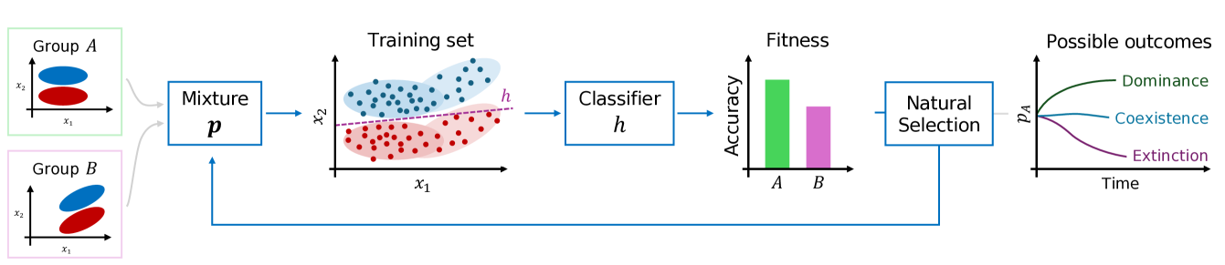
Figure 1: Interaction model in a two-group setting. Population is a mixture ${\bm{p}}$ of groups; Classifier $h$ is learned using data from the mixture distribution $D_{\bm{p}}$; Evolutionary fitness is associated with prediction accuracy; Differences in fitness drive change in mixture coefficients; Possible long-term outcomes are dominance (only $A$ survives), extinction (only $B$ survives), or coexistence (both survive).

1.1 Related Work

Our work relates to the emerging literature on performative prediction (Perdomo et al., 2020), which studies learning in settings where model deployments affect the underlying data distribution, with emphasis on (re)training dynamics and equilibrium. A central effort in this area is to identify global properties (e.g., appropriate notions of smoothness) that guarantee convergence. Our work complements this effort by proposing structure, in the form of evolutionary forces. This allows us to study a rich class of stateful performative dynamics, which are notoriously more challenging (Brown et al., 2022), thanks to an efficient low-dimensional representation of the distribution map (see Section A.1).

Evolutionary game theory was originally developed to model biological natural selection (Maynard Smith & Price, 1973), but has also been used in sociology (Bisin & Verdier, 2001) and financial markets (Scholl et al., 2021).The evolutionary prediction games we introduce are novel since they are defined as implicit solutions to statistical optimization problems. Our results for optimal classifiers reflect the principle of competitive exclusion (Hardin, 1960), while our analysis of non-optimal classifiers relates to long-studied questions of coexistence (e.g., Chesson, 2000).

Our formulation of evolutionary prediction games gives rise to a notion of equilibrium that satisfies the fairness criterion of overall accuracy equality in expectation (e.g., Verma & Rubin, 2018). Thus, rather than encouraging fair outcomes, we study a setting in which fairness is emergent. This adds another dimension to the question of fair outcomes, since it asks not only whether equity holds for the observed groups, but also which groups will remain to be observed. It also suggests an intriguing counterfactual perspective: if we observe fair outcomes at present, could this be because some groups were historically driven out of the game? This complements other voiced concerns regarding long-term outcomes of fair learning (Hashimoto et al., 2018; Liu et al., 2018; D’Amour et al., 2020).

2 Setting

The core of our setting is based on a standard supervised learning setup in which examples describe user data. Denote features by $x\in\mathcal{X}$ and labels $y\in\mathcal{Y}$. For a given distribution $D$ over pairs $(x,y)$, and given a training set $S={\left\{{(x_{i},y_{i})}\right\}}_{i=1}^{n}\sim D^{n}$, the goal in learning is to use $S$ to find a predictor $h:\mathcal{X}\to\mathcal{Y}$ from a class $\mathcal{H}$ which minimizes the expected error under some loss function $\ell:\mathcal{Y}\times\mathcal{Y}\to\mathbb{R}$. For concreteness, we focus primarily on classification tasks with the 0-1 loss, $\ell(\hat{y},y)=\mathds{1}\left\{{\hat{y}\neq y}\right\}$, whose minimization is equivalent to maximizing expected accuracy:

$$\mathrm{acc}_{D}(h)=\mathbb{P}_{(x,y)\sim D}{\left[{h(x)=y}\right]}$$ (1)

Denote the learning algorithm by $\mathcal{A}(S)$, and by $h\sim\mathcal{A}(D)$ the process mapping distributions to learned classifiers, with randomness due to sampling. Since solving Eq. (1) is both computationally and statistically hard, practical learning algorithms often resolve to optimizing an empirical surrogate loss (e.g., hinge or cross-entropy). One question we will ask is how such compromises affect long-term outcomes.

Population structure.

As data points $(x,y)$ are generated by users, the data distribution $D$ represents a population. We assume the population is a mixture of $K$ groups. Each group $k\in[K]$ is associated with a group-specific distribution $D_{k}$ over $(x,y)$ pairs, which remains fixed, and with a relative size $p_{k}$, which evolves over time. The overall data distribution is a mixture denoted by $D=D_{\bm{p}}=\sum_{k}p_{k}D_{k}$, where $p_{k}$ describes the relative proportion of group $k$ (such that $\sum_{k}p_{k}=1$ and $p_{k}\geq 0\,\,\forall k$). The population state vector ${\bm{p}}=(p_{1},\dots,p_{K})$ will be our main object of interest. Formally, the space of population states is the $(K-1)$-dimensional simplex $\Delta^{K}$. As ${\bm{p}}$ determines $D_{\bm{p}}$, for brevity we denote $h\sim\mathcal{A}({\bm{p}})=\mathcal{A}(D_{\bm{p}})$ and $\mathrm{acc}_{\bm{p}}(h)=\mathrm{acc}_{D_{\bm{p}}}(h)$. Our goal is to understand how changes in ${\bm{p}}$ affect learning, and in turn, how learning and its outcomes shape states ${\bm{p}}$.

Dynamics.

For a classifier $h\sim\mathcal{A}({\bm{p}})$, denote the marginal expected accuracy of $h$ on group $k$ by $\mathrm{acc}_{k}(h)=\mathrm{acc}_{D_{k}}(h)$. Informally, our central assumption on dynamics is that the proportion $p_{k}$ of each group $k$ grows if $\mathrm{acc}_{k}(h)$ is larger than others (on average), and shrinks if it is smaller. This aims to capture settings in which users benefit from accurate predictions, and so their tendency to use the system (or not) will depend on how well the system performs on other users in their cohort. Since $h$ is trained on the entire population, it is likely that some groups will benefit more (and therefore grow), and others less (and so will shrink). Thus, each deployment of a classifier induces change in ${\bm{p}}$, resulting in a form of distribution shift known as subpopulation shift (Yang et al., 2023). This, in turn, will influence the choice of classifier in the next time step—which forms a feedback loop between ${\bm{p}}$ and $h$. We propose to formalize and study such dynamics through the lens of evolutionary game theory, as described next.

3 Evolutionary Prediction Games

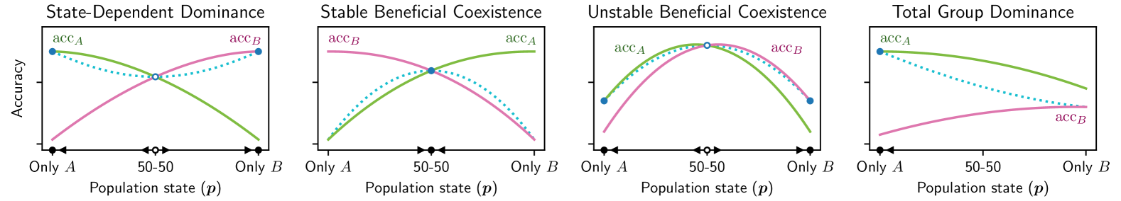
Figure 2: Graphical representation of two-group evolutionary prediction games (Definition 3.1). Groups are denoted by ${\left\{{A,B}\right\}}$. Solid lines describe expected group accuracies for each population state ${\bm{p}}$, dotted line describes population accuracy $\mathrm{acc}_{\bm{p}}(h)$, dots indicate Nash equilibria, and x-axis arrows indicate evolutionary stability. Each schematic diagram represents a possible scenario: (Left) State-dependent dominance. There are two stable equilibria, each dominated by a single group, with locally maximal population accuracy. Additionally, there is an unstable coexistence equilibrium. (Center Left) Stable beneficial coexistence. There is a stable coexistence equilibrium, with maximal population accuracy. (Center Right) Unstable beneficial coexistence. Coexistence has maximal population accuracy, but it is unstable. (Right) Total group dominance. There is a single equilibrium dominated by a single group.

Evolutionary Game Theory is a general framework for the analysis of natural selection processes (Maynard Smith & Price, 1973). The framework is built around population games – symmetric normal-form games for large number of agents, which model the interactions between $K$ species in a large mixed population. The population is modeled as a distribution over species ${\bm{p}}\in\Delta^{K}$. Each species $k\in[K]$ corresponds to a pure strategy in the population game, and is associated with a scalar fitness function, $F_{k}({\bm{p}})$, which quantifies its evolutionary fitness given population state ${\bm{p}}$. The fitness functions $F=\left(F_{1},\ldots,F_{K}\right)$ jointly define the population game, which then governs the dynamics of ${\bm{p}}$.

Learning as an evolutionary force.

We formalize the interplay between learning and user population dynamics through a novel type of population game, which we call an evolutionary prediction game. This game associates the fitness of each group with its expected marginal accuracy:

Definition 3.1 (Evolutionary Prediction Game).

Let $\mathcal{A}$ be a learning algorithm, and let $D_{1},\dots,D_{K}\in{\Delta\left({{\mathcal{X}\times\mathcal{Y}}}\right)}$ be group distributions. Denote by $\mathrm{acc}_{k}(h)$ the marginal accuracy of group $k\in[K]$ under classifier $h\sim\mathcal{A}({\bm{p}})$. The evolutionary fitness of group $k$ under population state ${\bm{p}}$ is:

$$F_{k}({\bm{p}})=\mathbb{E}_{h\sim\mathcal{A}({\bm{p}})}{\left[{\mathrm{acc}_{k}(h)}\right]}$$ (2)

Together, the fitness functions $F=(F_{1},\dots,F_{K})$ define an evolutionary prediction game over the population.

The game captures an implicit interaction between groups: While the fitness of each group $F_{k}({\bm{p}})$ is given by its own accuracy, the classifier $h$ is trained on the entire population, and thus different groups interact through the learning process. An illustration of this idea is outlined in Figure 1.

Dynamics revisited.

Our analysis considers the joint evolution of population states and classifiers. As population games may induce dynamics in several ways, we maintain generality by making only two structural assumptions on dynamics, namely that: (i) changes in $p_{k}$ are positively correlated with fitness $F_{k}({\bm{p}})$, and (ii) Nash equilibria of the population game are rest points of the dynamics. These hold for many well-known families of dynamical processes, including replicator dynamics (Taylor & Jonker, 1978), Moran processes (Moran, 1958), and multiplicative weight updates (e.g., Kleinberg et al., 2009) – See definitions in Section B.1. For the learning process, we first consider a setting where the classifier is trained only once at the onset (Section 4.1), and then proceed to study retraining dynamics in which $h$ is retrained at each step to fit the new distribution $D_{\bm{p}}$ (Sections 4.2, 5). This draws connections to the recent literature on performative prediction (Perdomo et al., 2020).

Evolutionary outcomes.

Denote the initial population state by ${\bm{p}}^{0}$, and the initial classifier by $h^{0}\sim\mathcal{A}({\bm{p}}^{0})$. We will be interested in characterizing the joint evolutionary outcomes of ${\bm{p}}$ and $h$. For the dynamics we consider, this takes the form of equilibrium points, denoted $({\bm{p}}^{*},h^{*})$. Games may have multiple equilibria, and the eventual outcome will depend on the group distributions, the learning algorithm, and the initial conditions. Our taxonomy of possible equilibria concerns three key properties:

• Survival: For the population, some groups may become extinct (e.g., $p^{*}_{k}\to 0$ for some $k\in[K]$), while others may reach coexistence (e.g., $p^{*}_{k}\to 1/K$ for all $k\in[K]$).

• Accuracy: For the classifier, natural selection may result in its performance improving over time, (i.e. $\mathrm{acc}(h^{*})>\mathrm{acc}(h^{0})$), deteriorating, or remaining unchanged.

• Stability: For the system, some equilibrium points will be robust to small perturbation of ${\bm{p}}^{*}$ and remain stable, while for others this may cause dynamics to diverge.

When $K=2$, the probability simplex $\Delta^{K}$ is equivalent to the unit interval $[0,1]$, and evolutionary prediction games admit a convenient graphical representation, illustrating the relations between the different elements (see Figure 2).

Nash equilibria and fairness.

For Nash equilibria, we follow the definition given by Sandholm (2010). Let $F({\bm{p}})$ be a population game. For a given population state ${\bm{p}}$, denote $\operatorname*{support}({\bm{p}})={\left\{{k\mid p_{k}>0}\right\}}$. A state ${\bm{p}}^{*}$ is a Nash equilibrium of $F({\bm{p}})$ if it satisfies the following condition:

$$\operatorname*{support}({\bm{p}}^{*})\subseteq\operatorname*{arg\,max}\nolimits_{k}F_{k}({\bm{p}}^{*})$$ (3)

We note that a Nash equilibrium exists for any population game (Sandholm, 2010, Thm. 2.1.1). In relation to fairness, we make the following connection (see Section B.2.2):

Proposition 3.2.

Let $F({\bm{p}})$ be an evolutionary prediction game induced by a learning algorithm $\mathcal{A}$, and let ${\bm{p}}^{*}$ be a Nash equilibrium. Then $\mathcal{A}$ satisfies the overall accuracy equality criterion in expectation when trained on $D_{{\bm{p}}^{*}}$.

4 Survival of the Fittest

4.1 Warm-up: Training Once

We begin with a characterization of evolutionary outcomes for a simple setting in which the classifier is trained only once on the initial distribution, and henceforth kept fixed. This is useful as a first step since, given the learned $h$, outcomes can be attributed solely to changes in the population.

Proposition 4.1.

Let $\mathcal{A}$ be a learning algorithm. Denote the initial population state by ${\bm{p}}^{0}$, and the initial classifier by $h^{0}\sim\mathcal{A}({\bm{p}}^{0})$. If $h^{0}$ is deployed at every time step (i.e., irrespective of the population state ${\bm{p}}$), then it holds that:

1. $\mathrm{acc}_{{\bm{p}}^{*}}(h^{0})\geq\mathrm{acc}_{{\bm{p}}^{0}}(h^{0})$

2. ${\bm{p}}^{*}$ is supported on $k^{*}=\operatorname*{arg\,max}_{k}\mathrm{acc}_{k}(h^{0})$

3. ${\bm{p}}^{*}$ is stable

Proof in Section B.3. Proposition 4.1 makes two important statements. First, from the perspective of the prediction system operator, overall accuracy only improves over time as a result of population dynamics. Since only group proportions ${\bm{p}}$ change, this improvement is due to an increase in $p_{k}$ for higher-accuracy groups, and a decrease for lower-accuracy groups. Thus, average accuracy increases—though not because of an actual ‘improvement’ in the model, but rather, due to the distribution becoming easier to predict.

Second, in the limit, this effect is driven to extreme, and a single group $k^{*}$—the one having the highest initial accuracy under $h^{0}$—will dominate at equilibrium ${\bm{p}}^{*}$. In evolution, this is known as the competitive exclusion principle (Hardin, 1960), which states that if multiple species compete over the same resources, then even a minimal advantage of one species over the others results in exclusive survival of the fittest species, and extinction of the rest.Our result suggests that this strong form of ‘survival of the fittest’ also applies to group dynamics driven by a fixed classifier.

Interpretation.

Although our results forecast that only the fittest will survive, it is important to remember that this describes outcomes in the limit. A more practical takeaway is that, as time progresses, the general tendency of the system will be for $p_{k^{*}}$ to gradually grow on account of others. If we wish to prevent eventual domination, then we should seek ways to intervene along the way. One possible approach is to retrain $h$, in hopes that this will lead to different outcomes: note that while accuracy under $h^{0}$ improves over time, the final $\mathrm{acc}_{{\bm{p}}^{*}}(h^{0})$ is by no means guaranteed to be the maximal attainable accuracy. Thus, working to continually improve accuracy should affect the eventual population. We now turn to study population dynamics under retraining.

4.2 Retraining Optimal Classifiers

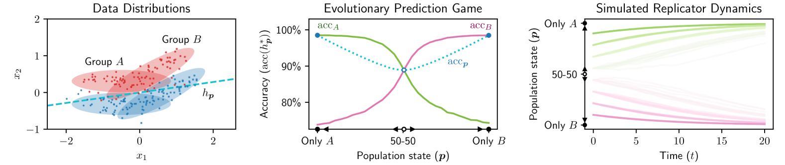
Figure 3: Evolutionary dynamics for two groups, induced by an optimal linear classifier (Section 4.2). (Left) Data distributions in feature space. Dashed line represents the optimal linear classifier $h_{\bm{p}}$ for the uniform mixture ${\bm{p}}=(0.5,0.5)$. (Center) Evolutionary prediction game induced by an optimal linear classifier. The game has two stable equilibria with single-group dominance, and one unstable coexistence equilibrium. Overall population accuracy $\mathrm{acc}_{\bm{p}}(h_{\bm{p}})$ is convex, and maximized at the stable equilibria. (Right) Replicator dynamics induced by the population game, for various initial conditions. Populations evolve towards states with single-group dominance.

To understand how populations and classifiers evolve jointly, we start by characterizing evolutionary outcomes for an ‘ideal’ setting in which the deployed classifier is optimal:

Definition 4.2 (Optimal classifier).

Let $\mathcal{H}$ be a hypothesis class, and let $D$ be a data distribution. An optimal classifier w.r.t. $\mathcal{H}$ is a minimizer of the 0-1 loss in expectation over $D$:

$$h^{\mathrm{opt}}\in\operatorname*{arg\,min}\nolimits_{h\in\mathcal{H}}\mathbb{E}_{(x,y)\sim D}{\left[{\mathds{1}\left\{{h(x)\neq y}\right\}}\right]}$$ (4)

Working with optimal classifiers abstracts away the complexities due to estimation and approximation errors of practical learning algorithms (i.e., algorithms that optimize proxy loss functions over finite data). Nonetheless, analyzing a dynamical system that is driven by the argmin of an expected objective remains quite challenging. We focus on settings in which $h^{\mathrm{opt}}$ exists, and denote by $\mathcal{A}^{\mathrm{opt}}({\bm{p}})$ the (theoretical) learning algorithm which returns the optimal classifier with respect to $D_{\bm{p}}$. In this case, the fitness function becomes $F_{k}({\bm{p}})=\mathrm{acc}_{k}\left(\mathcal{A}^{\mathrm{opt}}({\bm{p}})\right)$. We assume that fitness functions are differentiable, and that that ties are broken consistently if multiple optimal classifiers exist.

Our central theoretical result characterizes the possible evolutionary outcomes induced by optimal classifier retraining:

Theorem 4.3.

Let $\mathcal{H}$ be a hypothesis class, and denote by $\mathcal{A}^{\mathrm{opt}}$ the optimal learning algorithm w.r.t. $\mathcal{H}$. Fix an initial state ${\bm{p}}^{0}$, and assume that at each population state ${\bm{p}}$ the optimal classifier $h_{\bm{p}}\sim\mathcal{A}^{\mathrm{opt}}({\bm{p}})$ is deployed. Then it holds that:

1. Stable equilibria always exist. For all stable equilibria:

   • ${\left|{\operatorname*{support}({\bm{p}}^{*})}\right|}=1$

   • $\mathrm{acc}_{{\bm{p}}^{*}}\left(h_{{\bm{p}}^{*}}\right)\geq\mathrm{acc}_{{\bm{p}}^{0}}\left(h_{{\bm{p}}^{0}}\right)$

2. Unstable equilibria with ${\left|{\operatorname*{support}({\bm{p}}^{*})}\right|}>1$ may exist.

Proof in Section B.4. To prove the claim, we leverage basic structure which is revealed despite the complexity of the learning problem. Our main technical tool is the framework of potential games, which are population games that can be expressed as the gradient of a potential function. We first show that the expected accuracy of any fixed classifier is linear in ${\bm{p}}$. Then the core of the proof is a convexity argument: The optimality of $\mathcal{A}$ implies that $\mathrm{acc}_{\bm{p}}(h_{\bm{p}})$ is convex as a pointwise maximum of linear functions, with gradients given by marginal accuracies. From this we identify $\mathrm{acc}_{\bm{p}}(h_{\bm{p}})$ as the potential function for the game, and leverage the known correspondence between Nash equilibria of population games and extremal points of potential functions. Finally, the stability of single-population states follows from the fact that maximal points of convex functions over the simplex are attained at the vertices.

Interpretation.

Theorem 4.3 suggests multiple equilibria can exist, and distinguishes between two types. If dynamics converge to a stable equilibrium ${\bm{p}}^{*}$, then accuracy improves, but this is again through competitive exclusion, since $p^{*}_{k}>0$ for only one group. However, in contrast to training once, the surviving group is no longer predetermined, and can depend on context (e.g., initial state) and choices (e.g., model class). The more critical difference, however, is that retraining enables coexistence, in the form of possible equilibria in which multiple groups survive. That is, there may exist population states ${\bm{p}}^{*}$ such that $p^{*}_{k}>0$ for several groups $k$, and for which this remains to hold when the classifier is retrained. The crux, unfortunately, is that such points are inherently unstable, in the sense that any small perturbation of ${\bm{p}}^{*}$ will push dynamics away. Hence, under plausible dynamics, and for retraining with optimal classifiers, it is most unlikely that dynamics will converge to such states.

5 Avenues for Coexistence

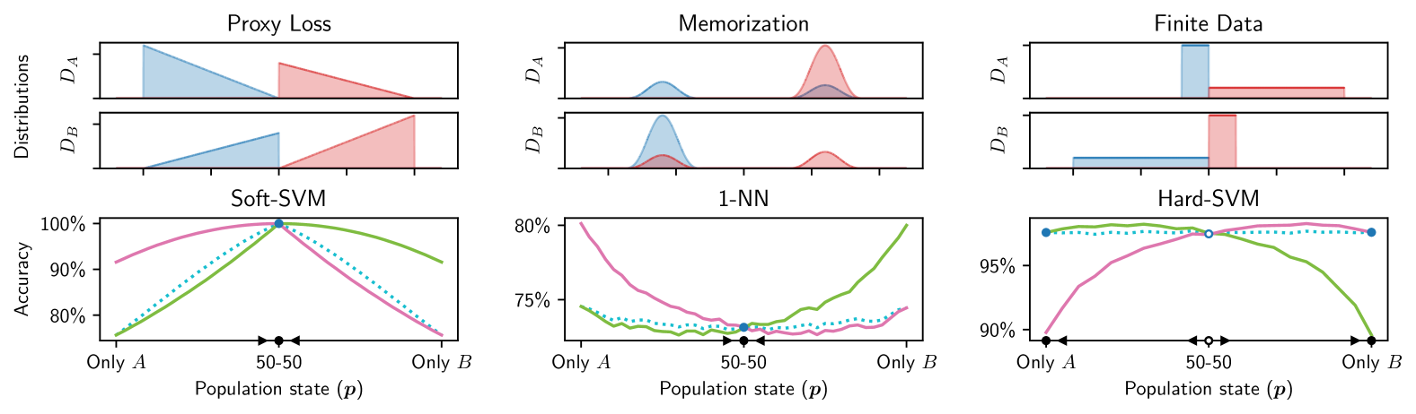
Figure 4: Graphical illustration of coexistence results. Top row presents data distributions, bottom row shows the corresponding prediction games. (Left) Stable and beneficial coexistence induced by the use of a proxy loss (Theorem 5.1). (Center) Stable coexistence induced by the use of memorization (Theorem 5.2). (Right) Beneficial coexistence induced by learning from a finite dataset (Theorem 5.3).

Intuitively, optimal classifiers drive dynamics away from mixture equilibria because the learning objective is fully aligned with, and so reinforces, fitness. But in practice we must resort to optimizing proxy empirical objectives, which can break alignment. This raises two important questions: when will mixture equilibria be stable, and can we make them such? For the first question, we show that each of the aspects which enable learning in practice—namely the use of proxy losses, finite data access, or memorization—can create conditions for coexistence to organically materialize. This entails coexistence that is beneficial (w.r.t. accuracy) stable, or both. For the second, we present preliminary steps.

5.1 Proxy Loss

A common approach to overcoming the difficulty due to the discontinuity of the 0-1 loss is to replace it with a convex surrogate defined over predictive scores. This enables optimization, but introduces bias: for example, instead of a uniform penalty of 1, misclassified points are penalized relative to their distance from the decision boundary of $h$. Our next result shows that this limitation enables coexistence if the two groups have opposing biases, which balance at equilibrium. The construction relies on the Soft-SVM algorithm which uses the hinge loss with $\ell_{2}$ regularization.

Theorem 5.1.

For the Soft-SVM algorithm, there exist data distributions that induce an evolutionary prediction game with a mixture equilibrium that is both stable and beneficial.

Proof in Section B.5, and the construction is outlined in Figure 4 (Left). The main idea of the construction is to leverage the bias of Soft-SVM against the minority class in imbalanced settings. For each group alone, minimizing the proxy loss biases the learned classifier against the minority class, which is suboptimal. However, when both groups coexist, these biases cancel out. The surprising property is that when one group grows slightly (e.g., $p_{1}=0.5+\epsilon$), it loses more from the fact that the other group shrinks (e.g., $p_{2}=0.5-\epsilon$) than it gains from its own growth. This symbiotic relation leads to stable and beneficial coexistence. In Section B.5.3, we expand on this idea, showing that varying the SVM regularization parameter leads to bifurcations in which the game transitions between 3, 1, and 5 equilibria.

5.2 Memorization

Another practical approach to loss minimization is to use a class of models that fit the training data perfectly and then interpolate. Notable examples $k$-NN and overparameterized neural networks (e.g., Zhang et al., 2021). Memorization leads to zero loss on the training set by definition, but often at the price of sensitivity to noise; as a concrete example, consider how 1-NN predictions change with the addition of a single point. The problem is that even in the limit, 1-NN cannot express the true $p(y|x)$, and remains sensitive to label noise. Our next result shows this can lead to coexistence:

Theorem 5.2.

For the 1-NN learning algorithm, there exist noisy-label data distributions that induce an evolutionary prediction game with stable coexistence.

Proof in Section B.6, and the construction is illustrated in Figure 4 (Center). The key property leveraged by this proof is asymmetric label noise. There are two groups defined symmetrically. Each group is composed of a majority and minority classes, and the majority class has label noise. For each group alone, the 1-NN algorithm makes perfect predictions on its minority class, and imperfect predictions on the majority class. Since groups are defined symmetrically, training on one group alone leads to better accuracy for the other—leading to stable coexistence. Section B.6.2 shows that under $k>1$, stable coexistence can also be beneficial.

5.3 Finite data

All practical learning algorithms must rely on a finite sample of data points for training a classifier. Learnability (in the PAC sense) implies that as data size grows, the sample becomes increasingly representative of the distribution. But the rate at which variance diminishes need not be equally across all regions of a distribution. In a sense, this means that one region can be learned ‘faster’ (i.e., with less data) than another. Our final example exploits this to show how coexistence can arise from statistical considerations.

Theorem 5.3.

For the Hard-SVM algorithm, there exist linearly-separable data distributions induce an evolutionary prediction game with beneficial coexistence.

Proof in Section B.7, and the construction is illustrated in Figure 4 (Right). The key property we leverage here is asymmetric class variance. In each group, one class has high variance, and the other class has low variance. When the dataset is finite (of size $n$), this creates bias against the high-variance class, and thus convergence towards the optimal classifier at a linear rate ($O(n^{-1})$). When the two groups coexist, this bias is balanced, and the rate of convergence is exponential—leading to beneficial coexistence. The crux in the construction is that while coexistence is beneficial, it is unstable. Generally we suspect that stability is difficult to obtain through pure statistical means. But this does not mean that it is generally unattainable, as we show next.

5.4 Stabilizing Coexistence Equilibria

We have thus far considered retraining with the objective of maximizing accuracy at each time step on the current distribution. But if the learner is aware of population dynamics, then this can be leveraged in training. Our next result shows that it is possible to turn an unstable equilibrium into a stable one by simple reweighing of the accuracy objective:

Proposition 5.4.

Let $\mathcal{A}({\bm{p}})$ be an optimal algorithm with equilibrium ${\bm{p}}^{*}$. If ${\bm{p}}^{*}$ has full support (and thus is unstable), then it becomes stable under $\mathcal{A}^{\prime}({\bm{p}})=\mathcal{A}(2{\bm{p}}^{*}-{\bm{p}})$.

Proof in Section B.8. The idea is that $\mathcal{A}^{\prime}$ trains ‘as if’ the state is $2{\bm{p}}^{*}-{\bm{p}}$, which can be achieved by weighing examples from each group $k$ by $w_{k}=\frac{p_{k}}{2p^{*}_{k}-p_{k}}$. This inverts the natural tendency of dynamics to push away from the unstable equilibrium, and instead pull towards it.

6 Empirical Evaluation

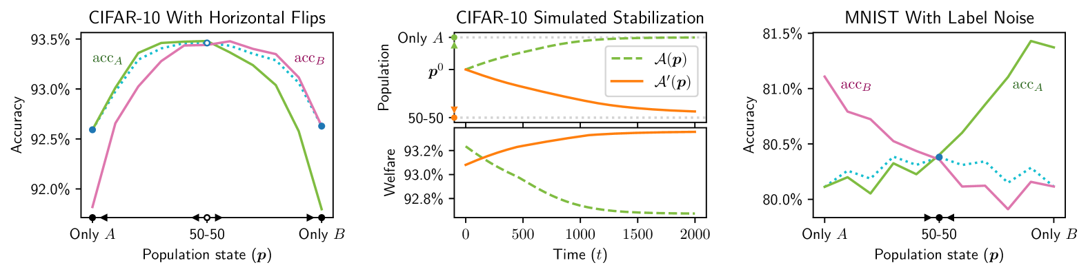
Figure 5: Empirical evaluation results. (Left) Evolutionary prediction game induced by CIFAR-10 with Resnet-9 and groups representing horizontal flips. The game has beneficial unstable coexistence (Section 6.1). (Center) Simulated stabilization of replicator dynamics on the CIFAR-10 game (Section 5.4). (Right) Game induced by MNIST with label noise, showing stable beneficial coexistence (Section 6.2).

We now turn to explore evolutionary prediction games empirically using real data and simulated dynamics.

6.1 Beneficial Coexistence Through Data Augmentation

Our first empirical result explores an avenue for beneficial coexistence inspired by data augmentation techniques. Data augmentations enrich the training set with class-preserving transformations of inputs. These serve as a proxy for additional data that is representative of the task but is unbounded to the biases specific to the observed data distribution (e.g., camera angle, source of lighting). Such relations can occur naturally: for example, medical images from different hospitals may differ in imaging device calibration, and pooling them together can provide robustness.

Method.

We use the CIFAR-10 image recognition dataset (Krizhevsky, 2009), which consists of 60000 32x32 color images in 10 classes, with 6000 images per class. As horizontal image flips are considered class-preserving for this dataset, group $A$ consists of images sampled directly from CIFAR-10, and group $B$ consists of images under horizontal flip. We use a ResNet-9 network for prediction (He et al., 2016), and train it using the ffcv framework with default optimization parameters (Leclerc et al., 2023). For each ${\bm{p}}$ we measure the prediction model’s accuracy on the original images from the CIFAR test set (representing $\mathrm{acc}_{A}(h_{\bm{p}})$), and on their flipped counterparts (representing $\mathrm{acc}_{B}(h_{\bm{p}})$). For stabilization, we use the method described in Proposition 5.4 with ${\bm{p}}^{*}=(0.5,0.5)$. We simulate the evolutionary process using discrete replicator dynamics, and use linear interpolation due determine intermediate fitness values.

Results.

A graphical representation of the estimated evolutionary prediction game is presented in Fig. 5 (Left). The game has three equilibria: Two stable equilibria with single-group dominance ($92.6\%{}$ accuracy), and an unstable coexistence equilibrium ($93.5\%{}$ accuracy). Fig. 5 (Center) shows how stabilization induces stable beneficial coexistence.

6.2 Stable Coexistence Through Overparameterization

Our second empirical result explores an avenue for stable coexistence driven by properties of overparametrized neural networks. Modern neural networks are frequently overparameterized, and are known to achieve strong test-time performance despite memorizing the training data (e.g., Zhang et al., 2021). Recent research attributes this phenomenon to the implicit biases introduced by the training process (e.g., Vardi, 2023). Building on the ideas presented in Theorem 5.3, we demonstrate that stable coexistence can emerge when an overparameterized neural network is trained on a multi-class classification task with label noise.

Method.

We use the MNIST dataset for digit recognition (LeCun, 1998), which consists of 70000 28x28 grayscale images of handwritten digits across 10 classes. Each class is split unevenly between the two groups: Group $A$ is biased towards even digits ${\left\{{0,2,4,6,8}\right\}}$, and group $B$ is biased towards odd digits, both with a 4:1 imbalance. For each group, we introduce label noise to the majority classes, mapping the true label of each digit $d$ to the next digit with same parity with probability $0.2$ (i.e. for group $A$, label noising stochastically maps $0\mapsto 2$, $2\mapsto 4$, etc.). We train a convolutional neural network for 200 epochs using stochastic gradient decent with momentum. The training and test sets are split independently, and for each ${\bm{p}}$ we measure the prediction model’s accuracy on both splits of the test sets (representing $\mathrm{acc}_{A}(h_{\bm{p}})$ and $\mathrm{acc}_{B}(h_{\bm{p}})$). Under the given parameters, the label noising process leads to an accuracy upper bound of $84\%$ assuming perfect recognition.

Results.

A graphical representation of the estimated evolutionary prediction game is presented in Figure 5 (Right). The game has a single beneficial coexistence equilibrium with accuracy $80.4\%{}$ (c.f. the $84\%$ test accuracy upper bound due to label noise). In addition, we observe an average training accuracy of $98.7\%{}$, indicating memorization.

7 Discussion

The study of population dynamics is central to biology and ecology, a task for which population games have proven to be highly effective. We believe there is need to ask similar questions regarding the dynamics of social populations, as they become increasingly susceptible to the effects of predictive learning algorithms. The social world is of course quite distinct from the biological, but there is nonetheless much to gain from adopting an ecological perspective. One implication of our results is that, without intervention, learning might drive a population of users to states which would otherwise be unfavorable. Ecologists address such problems by studying and devising tools for effective conservation. Similar ideas can be used in learning for fostering and sustaining heterogeneous user populations. Our work intends to stir discussion about such ideas within the learning community.

Impact statement

Our work seeks to shed light on the question: how does the deployment of learned classifier impact the long-term composition of the population of its users? Posing this question as one of equilibrium under a novel population game, our results describe the possible evolutionary outcomes under simple conditions (training once), optimal conditions (perfect classifiers), and realistic settings (namely empirical surrogate loss minimization). The fact that learning can influence population dynamics can have major implications on social and individual outcomes. Our work intends to illuminate this aspect of learning in social contexts, and to provide a basic and preliminary understanding of such interactions.

The bulk of our results are theoretical in nature, and as such, rely on several assumptions. Some regard the learning process: for example, we consider only simple accuracy-maximizing algorithms that optimize over a fixed-size training set sampled only from the current (and not past) data distribution. Others concern dynamics: for example, we assume no exogenous forces (i.e., which could prevent extinction), intra-group distribution shifts, or inter-group dependencies (other than those indirectly formed through the classifier). Whether our results hold also when these assumptions are relaxed is an important future question.

It is also important to interpret our results appropriately and with care. For example, statements which establish ‘extinction’ as a likely outcome apply only limiting behavior, and so are silent on trajectories, rates, or any finite timepoint. Our results also rely on users being partitioned into non-overlapping groups. In reality, group memberships are rarely exclusive (or even fixed), and the dependence of individual behavior on group outcomes (in our case, marginal group accuracy—which defines fitness) is unlikely to be strict.

The above points should be considered when attempting to draw conclusions from our theoretical results to real learning problems. However, and despite these limitations, we believe the message we convey—which is that learning in social settings requires intervention and conservation to ensure sustainability of social groups and individuals—applies broadly and beyond our framework’s scope.

Appendix A Further Discussion of Related Work

A.1 Relation to Performative Prediction

Performative prediction (Perdomo et al., 2020) is a general framework for modeling the effects of predictive models on the data distributions they are tested and trained on. In particular, stateful performative prediction (Brown et al., 2022) generalizes the original framework to model stateful performative dynamics. In the stateful framework, the performative effects of a predictor $h\in\mathcal{H}$ are formally modeled using a stateful transition function $D_{t+1}=T(D_{t},h)$, where $D_{t},D_{t+1}\in{\Delta\left({{\mathcal{X}\times\mathcal{Y}}}\right)}$ are the data distributions at times $t,t+1$, and $h\in\mathcal{H}$ is the predictor being deployed. We note that the space of feature-label distributions is infinite-dimensional under the common assumption $\mathcal{X}\subseteq\mathbb{R}^{d}$. Additionally, we note that the space of classifiers $\mathcal{H}$ is high-dimensional when the hypotheses class $\mathcal{H}$ is complex (e.g., a class of deep neural networks). Thus, the general framework allows for transition operators which are infinite-dimensional (e.g., as noted by Conger et al., 2024).

In the context of performative prediction, our setting can be seen as a special case of stateful performative prediction, where the transition operator $T$ operates within a low-dimensional subspace of all possible feature label-distributions (mixtures of fixed distributions), and depends on predictors through low-dimensional statistics (their marginal accuracy on each group). Formally, given a collection of group distributions $D_{1},\dots,D_{K}\in{\Delta\left({{\mathcal{X}\times\mathcal{Y}}}\right)}$, denote the space of mixtures by $\Delta_{\mathrm{mix}}={\left\{{\sum_{k}\alpha_{k}D_{k}\mid\alpha\in{\Delta\left({[K]}\right)}}\right\}}$, and note that $\Delta_{\mathrm{mix}}\subseteq{\Delta\left({{\mathcal{X}\times\mathcal{Y}}}\right)}$. By definition, any mixture $D\in\Delta_{\mathrm{mix}}$ can be represented using a $(K-1)$-dimensional vector ${\bm{p}}\in{\Delta\left({[K]}\right)}$. Additionally, as performative response is assumed to depend on predictor accuracy, the transition operator depends on the classifier $h$ through a $K$-dimensional vector of accuracies $\mathbf{acc}(h)=\left(\mathrm{acc}_{1}(h),\dots,\mathrm{acc}_{K}(h)\right)\in\left[0,1\right]^{K}$. Therefore, transition operators induced by the evolutionary model can be seen as mappings ${\bm{p}}^{\prime}=T({\bm{p}},\mathbf{acc}(h))$ from a $(2K-1)$-dimensional space to a $(K-1)$-dimensional space.

Appendix B Deferred Proofs

B.1 Preliminaries

Distributions.

The set of distribution over a set $A$ is denoted by ${\Delta\left({A}\right)}$, and the set of distributions over $[K]$ is denoted by $\Delta^{K}={\Delta\left({[K]}\right)}={\left\{{{\bm{p}}\mid\sum_{k}p_{k}=1,p_{k}\geq 0\ \ \forall k\in[K]}\right\}}$. Following the notations in Sandholm (2010), we denote the space tangent to the $K$-simplex by $T\Delta^{K}={\left\{{z\in\mathbb{R}^{K}\mid\sum_{k}z_{k}=0}\right\}}$. We denote ${\bm{1}}=\left(1,\dots,1\right)\in\mathbb{R}^{K}$, and denote by ${\bm{\Phi}}={\bm{I}}-{\bm{1}}{\bm{1}}^{T}$ the orthogonal projection matrix from $\mathbb{R}^{K}$ to $T\Delta^{K}$.

Supervised learning.

We denote the space of features by $\mathcal{X}$, the space of labels by $\mathcal{Y}$, the hypotheses class by $\mathcal{H}\subseteq\mathcal{Y}^{\mathcal{X}}$, and the loss function by $\mathcal{L}:\mathcal{Y}^{2}\to\mathbb{R}$. The expected loss of hypothesis $h\in\mathcal{H}$ under population distribution $D\in{\Delta\left({{\mathcal{X}\times\mathcal{Y}}}\right)}$ is denoted by $\mathcal{L}_{D}(h)=\mathbb{E}_{(x,y)\sim D}{\left[{\mathcal{L}(h(x),y)}\right]}$. A supervised learning algorithm $\mathcal{A}$ is a stochastic mapping from a distribution $D\in{\Delta\left({{\mathcal{X}\times\mathcal{Y}}}\right)}$ to a classifier $h\sim\mathcal{A}(D)$, formally $\mathcal{A}:{\Delta\left({{\mathcal{X}\times\mathcal{Y}}}\right)}\to{\Delta\left({\mathcal{H}}\right)}$.

Population state.

Each group $k$ is associated with a feature-label distribution $D_{k}\in{\Delta\left({{\mathcal{X}\times\mathcal{Y}}}\right)}$. For a population state ${\bm{p}}\in\Delta^{K}$, the population mixture distribution is denoted by $D_{\bm{p}}=\sum_{k\in[K]}p_{k}D_{k}$. We use a vector subscript notation to distinguish between group distributions (e.g. $D_{k}$) and mixture distributions (e.g. $D_{\bm{p}}$). For a hypothesis $h\in\mathcal{H}$, the expected loss of group $k$ is denoted by $\mathcal{L}_{k}(h)=\mathbb{E}_{(x,y)\sim D_{k}}{\left[{\mathcal{L}(h(x),y)}\right]}$, and the vector of expected group losses is denoted by $\vec{\mathcal{L}}(h)=\left(\mathcal{L}_{1}(h),\dots,\mathcal{L}_{K}(h)\right)$. For ${\bm{p}}\in\Delta^{K}$, the expected loss of $h$ under distribution $D_{\bm{p}}$ is denoted by $\mathcal{L}_{\bm{p}}(h)=\mathbb{E}_{(x,y)\sim D_{\bm{p}}}{\left[{\mathcal{L}(h(x),y)}\right]}$. The support of a population state ${\bm{p}}$ is denoted by $\operatorname*{support}({\bm{p}})={\left\{{k\in[K]\mid p_{k}>0}\right\}}$.

Population games.

We follow the notations of Sandholm (2010), and provide the key definitions here for completeness. Population games associate each group $k\in[K]$ with a fitness function $F_{k}({\bm{p}})$, which maps a population state ${\bm{p}}\in\Delta^{K}$ to the evolutionary fitness of group $k$. A Nash Equilibrium (NE) of a population game is a population state ${\bm{p}}^{*}$ which satisfies $\operatorname*{support}({\bm{p}}^{*})\subseteq\operatorname*{arg\,max}_{k\in[K]}F_{k}({\bm{p}}^{*})$, and we note that every population game admits at least one Nash equilibrium (Sandholm, 2010, Theorem 2.1.1).

Evolutionary dynamics.

For population dynamics, we make the positive correlation assumption (Sandholm, 2010, Section 5.2), and assume that whenever a population is not at rest, the growth rate of a group is positively correlated with its fitness. Positive correlation implies that all Nash equilibria are rest points of the dynamics (Sandholm, 2010, Proposition 5.2.1). For our simulations, we use the replicator dynamics (Taylor & Jonker, 1978), which satisfy this property. We also note that other dynamics converge towards the replicator dynamics in the limit – For example, Moran in the large-population limit (Traulsen et al., 2006), and multiplicative-weights as the multiplicative factor approaches $1$ and time is renormalized accordingly (e.g., Kleinberg et al., 2011). To simplify analysis, we assume that all groups are present at the onset (${\left|{\operatorname*{support}({\bm{p}}^{0})}\right|}=K$).

Potential games.

A population game is a potential game if it can be represented as a gradient of some function. Formally, $F:\Delta^{K}\to\mathbb{R}^{K}$ is a potential game if there exists $f:\Delta^{K}\to\mathbb{R}$ such that $F=\nabla f$, where $\nabla f$ is the gradient of $f$ over the simplex (see Sandholm, 2010, Section 3.2 for rigorous definitions). We informally state key results that are relevant to our setting: By (Sandholm, 2010, Theorem 3.1.3), a state ${\bm{p}}^{*}$ is a Nash equilibrium of $F$ if and only if it is an extremum of the potential function $f$. By (Sandholm, 2010, Theorem 7.1.2), dynamics satisfying the positive correlation property converge towards Nash equilibria (restricted Nash equilibria in case of replicator dynamics). Finally, by (Sandholm, 2010, Theorem 8.2.1), a population state ${\bm{p}}^{*}$ is a stable equilbrium if and only if it is a local maximizer of $f({\bm{p}})$.

B.2 Basic Claims

B.2.1 Linearity

Proposition B.1 (Expected loss is linear in ${\bm{p}}$ for a fixed hypothesis).

For any $h\in\mathcal{H}$ and ${\bm{p}}\in\Delta^{K}$, The expected loss can be represented as a convex combination:

$$\mathcal{L}_{\bm{p}}(h)=\sum_{k\in[K]}p_{k}\cdot\mathcal{L}_{k}(h)$$

Proof.

Given a population state ${\bm{p}}$, treat it as a categorical random variable over population groups, denote by $k\sim{\bm{p}}$ the group from which a feature-label pair gets selected. Applying the law of total expectation and using the definition of $\mathcal{L}_{\bm{p}}(h)$, we obtain:

$$\mathcal{L}_{\bm{p}}(h) =\mathbb{E}_{(x,y)\sim D_{\bm{p}}}{\left[{\mathcal{L}(h(x),y)}\right]}$$

$$=\mathbb{E}_{k\sim{\bm{p}}}{\left[{\mathbb{E}_{(x,y)\sim D_{k}}{\left[{\mathcal{L}(h(x),y)}\right]}}\right]}$$

$$=\sum_{k\in[K]}p_{k}\cdot\mathbb{E}_{(x,y)\sim D_{k}}{\left[{\mathcal{L}(h(x),y)}\right]}$$

$$=\sum_{k\in[K]}p_{k}\cdot\mathcal{L}_{k}(h)$$

∎

B.2.2 Overall accuracy equality

A classifier $h$ satisfies overall accuracy equality if both protected and unprotected groups have equal prediction accuracy. In the context of natural selection, we consider this definition with respect to the groups currently present in the population:

Definition B.2 (Overall accuracy equality; (e.g., Verma & Rubin, 2018)).

Let $h:\mathcal{X}\to\mathcal{Y}$, and let ${\bm{p}}\in\Delta^{K}$ be a population state. $h$ satisfies overall prediction equality if $\mathrm{acc}_{k}(h)=\mathrm{acc}_{k^{\prime}}(h)$ for all $k,k^{\prime}\in\operatorname*{support}({\bm{p}})$.

Under retraining, a different classifier is deployed at each time step. It is therefore natural to define this property with respect to the learning algorithm, rather than a single classifier. In the definition, we take the expectation over the stochasticity of the sampling and learning process to representing the average over time under retraining:

Definition B.3 (Overall accuracy equality in expectation).

Let ${\bm{p}}$ be a population state, and let $\mathcal{A}({\bm{p}})$ be a learning algorithm. $\mathcal{A}$ satisfies overall prediction equality in expectation if $\mathbb{E}_{h\sim\mathcal{A}({\bm{p}})}{\left[{\mathrm{acc}_{k}(h)}\right]}=\mathbb{E}_{h\sim\mathcal{A}(D)}{\left[{\mathrm{acc}_{k^{\prime}}(h)}\right]}$ for all $k,k^{\prime}\in\operatorname*{support}({\bm{p}})$.

Proof of Proposition 3.2.

Let ${\bm{p}}^{*}$ be a Nash equilibrium of the evolutionary prediction game induced by $\mathcal{A}({\bm{p}})$. By Equation 3, it holds that $\operatorname*{support}({\bm{p}}^{*})\subseteq\operatorname*{arg\,max}_{k}F_{k}({\bm{p}}^{*})$, and therefore there exists some $a\in\mathbb{R}$ such that $F_{k}({\bm{p}}^{*})=a$ for all $k\in\operatorname*{support}({\bm{p}}^{*})$. Then by the definition of the evolutionary prediction game (Definition 3.1), it holds that: $\mathbb{E}_{h\sim\mathcal{A}({\bm{p}})}{\left[{\mathrm{acc}_{k}(h)}\right]}=\mathbb{E}_{h\sim\mathcal{A}(D)}{\left[{\mathrm{acc}_{k^{\prime}}(h)}\right]}=a$ for all $k,k^{\prime}\in\operatorname*{support}({\bm{p}}^{*})$. ∎

B.3 Training Once

Definition B.4 (Train-once prediction game).

Let ${\bm{p}}^{0}\in\Delta^{K}$ be the population state at time 0, and denote by $h^{0}\in\mathcal{H}$ the hypothesis learned at time 0. The train-once prediction game is a population game with the following fitness function:

$$F_{k}({\bm{p}};h^{0})=-\mathcal{L}_{k}(h^{0})$$

Definition B.5 (Constant game; (Sandholm, 2010, Section 3.2.4)).

A population game $F:\Delta^{K}\to\mathbb{R}^{K}$ is a constant game if there exist constants $\alpha_{1},\dots,\alpha_{K}\in\mathbb{R}$ such that $F_{k}({\bm{p}})=\alpha_{k}$ for all ${\bm{p}}\in\Delta^{K}$.

Proposition B.6.

let $\mathcal{L}$ be a loss function, let ${\bm{p}}^{0}\in\Delta^{K}$ be the population state at time 0, and let $h^{0}\in\mathcal{H}$ be the hypothesis learned at time 0. Denote by $F_{k}({\bm{p}})$ the corresponding train-once prediction game, and denote by ${\bm{p}}^{*}$ a Nash equilibrium of $F$. It holds that:

1. $\operatorname*{support}({\bm{p}}^{*})\subseteq\operatorname*{arg\,min}_{k\in[K]}\mathcal{L}_{k}(h^{0})$

2. $\mathcal{L}_{{\bm{p}}^{*}}(h)\leq\mathcal{L}_{{\bm{p}}^{0}}(h)$

3. ${\bm{p}}^{*}$ is stable.

Proof.

Fix $h_{0}\in\mathcal{Y}^{\mathcal{X}}$. In the train-once setting, the expected marginal accuracies are constant as a function of ${\bm{p}}$, and therefore $F_{k}$ is a constant game by Definition B.5. By (Sandholm, 2010, Proposition 3.2.13), $F_{k}$ a potential game with linear potential $f({\bm{p}})=-\vec{\mathcal{L}}(h^{0})\cdot{\bm{p}}$. By (Sandholm, 2010, Theorem 3.1.3), the set of Nash equilibria is the set of local maximizers of $f({\bm{p}})$, which is a convex combination over the set $\operatorname*{arg\,min}_{k\in[K]}\mathcal{L}_{k}(h^{0})$ due to linearity. Hence:

$$\operatorname*{support}({\bm{p}}^{*})\subseteq\operatorname*{arg\,min}_{k\in[K]}\mathcal{L}_{k}(h^{0})$$

satisfying (1).

At equilibrium ${\bm{p}}^{*}$, it holds that $\mathcal{L}_{{\bm{p}}^{*}}=\min_{k\in[K]}\mathcal{L}_{k}(h^{0})$. Apply Proposition B.1 to obtain:

$$\mathcal{L}_{{\bm{p}}^{0}}(h^{0}) =\sum_{k}p_{k}^{0}\mathcal{L}_{k}(h^{0})$$

$$\geq\sum_{k}p_{k}^{0}\min_{k^{\prime}\in[K]}\mathcal{L}_{k^{\prime}}(h^{0})$$

$$=\min_{k^{\prime}\in[K]}\mathcal{L}_{k^{\prime}}(h^{0})$$

$$=\mathcal{L}_{{\bm{p}}^{*}}(h^{0})$$

satisfying (2).

Finally, observe that each ${\bm{p}}^{*}$ is stable as a maximizer of the linear potential function (Sandholm, 2010, Theorem 8.2.1). ∎

Proof of Proposition 4.1.

Proposition 4.1 is a special case of Proposition B.6 for the loss function: $\mathcal{L}_{k}(h)=-\mathrm{acc}_{k}(h)$. ∎

B.4 Retraining

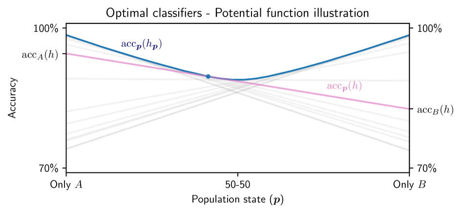
Figure 6: Theorem 4.3 – Illustration of the proof. Pink line: The expected accuracy of a fixed classifier $h$ is linear in ${\bm{p}}$ (Proposition B.1). Blue line: The overall accuracy of the optimal classifier $h_{\bm{p}}$ is a pointwise maximum over linear functions, and is therefore convex (Proposition B.9). The gradient of $\mathrm{acc}_{\bm{p}}(h_{\bm{p}})$ over the simplex is the vector of marginal accuracies, showing that the overall accuracy is a potential function for the game (Proposition B.12). Properties of the game’s equilibria then follow from convexity arguments.

Definition B.7 (Retraining prediction game with an optimal predictor).

Let ${\bm{p}}\in\Delta^{K}$, let $\mathcal{L}$ be a loss function, and let $\mathcal{H}$ be a hypothesis class. Denote $h_{\bm{p}}\in\operatorname*{arg\,min}_{h\in\mathcal{H}}\mathcal{L}_{\bm{p}}(h)$, and assume ties are broken in a consistent way. The retraining prediction game with an optimal predictor is a population game with the following payoff function:

$$F_{k}({\bm{p}})=-\mathcal{L}_{k}(h_{\bm{p}})$$

Definition B.8 (Optimal loss function $l^{*}({\bm{p}})$).

Given hypotheses $\mathcal{H}$ and population state ${\bm{p}}\in\Delta^{K}$, the optimal loss at ${\bm{p}}$ is:

$$l^{*}({\bm{p}})=\min_{h\in\mathcal{H}}\mathcal{L}_{\bm{p}}(h)$$

Proposition B.9 ($l^{*}({\bm{p}})$ is concave).

The optimal loss $l^{*}({\bm{p}})$ is a concave function of ${\bm{p}}$.

Proof.

By definition of $l^{*}({\bm{p}})$:

$$l^{*}({\bm{p}})=\min_{h\in\mathcal{H}}\mathcal{L}_{\bm{p}}(h)$$

From Proposition B.1, each $\mathcal{L}_{\bm{p}}(h)$ is linear in ${\bm{p}}$ for all $h\in\mathcal{H}$, and in particular concave. Hence, $l^{*}({\bm{p}})$ is a point-wise minimum of concave functions, and is therefore concave. ∎

Definition B.10 (Subgradient; (e.g., Rockafellar, 1970, Section 23)).

Let $f:\Delta^{K}\to\mathbb{R}$ be a convex function over the simplex. The vector ${\bm{v}}\in T\Delta^{K}$ is a subgradient of $f$ at point ${\bm{p}}$ if for all ${\bm{p}}^{\prime}$ it holds that:

$$f({\bm{p}})+{\bm{v}}\cdot({\bm{p}}^{\prime}-{\bm{p}})\leq f({\bm{p}}^{\prime})$$

Where $f({\bm{p}})+{\bm{v}}\cdot({\bm{p}}^{\prime}-{\bm{p}})$ is the tangent plane at point ${\bm{p}}$.

Definition B.11 (Subdifferential).

Let $f:\Delta^{K}\to\mathbb{R}$ be a convex function over the simplex. The subdifferential of $f$ at ${\bm{p}}$ is set of all subgradients at point ${\bm{p}}$, denoted by $\partial f({\bm{p}})$.

Proposition B.12.

Let $h_{\bm{p}}\in\operatorname*{arg\,min}_{h\in\mathcal{H}}\mathcal{L}_{\bm{p}}(h)$ be an optimal predictor. The projection of the loss vector of $h$ at point ${\bm{p}}$ is a subgradient of $-l^{*}({\bm{p}})$:

$${\bm{\Phi}}\vec{\mathcal{L}}(h_{\bm{p}})\in\partial\left(-l^{*}({\bm{p}})\right)$$

Proof.

Let $h_{\bm{p}}\in\operatorname*{arg\,min}_{h\in\mathcal{H}}\mathcal{L}_{\bm{p}}(h)$, and let ${\bm{p}},{\bm{p}}^{\prime}\in\Delta^{K}$. We need to show that $-l^{*}({\bm{p}})+\vec{\mathcal{L}}(h_{\bm{p}})\cdot({\bm{p}}^{\prime}-{\bm{p}})\leq-l^{*}({\bm{p}}^{\prime})$.

By Proposition B.1, it holds that $\mathcal{L}_{{\bm{p}}^{\prime}}(h_{\bm{p}})=\sum_{k}p^{\prime}_{k}\mathcal{L}_{k}(h_{\bm{p}})$. By algebraic manipulation we obtain:

$$\mathcal{L}_{{\bm{p}}^{\prime}}(h_{\bm{p}}) =\vec{\mathcal{L}}(h_{\bm{p}})\cdot{\bm{p}}^{\prime}$$ (5)

$$=\overbrace{\underbrace{\vec{\mathcal{L}}(h_{\bm{p}})\cdot{\bm{p}}}_{=l^{*}({\bm{p}})}-\vec{\mathcal{L}}(h_{\bm{p}})\cdot{\bm{p}}}^{=0}+\vec{\mathcal{L}}(h_{\bm{p}})\cdot{\bm{p}}^{\prime}$$

$$=l^{*}({\bm{p}})+\vec{\mathcal{L}}(h_{\bm{p}})\cdot\left({\bm{p}}^{\prime}-{\bm{p}}\right)$$

As ${\bm{p}}^{\prime}-{\bm{p}}\in T\Delta^{K}$, it is not affected by the orthogonal projection ${\bm{\Phi}}:\mathbb{R}^{K}\to T\Delta^{K}$:

$${\bm{\Phi}}\left({\bm{p}}^{\prime}-{\bm{p}}\right)={\bm{p}}^{\prime}-{\bm{p}}$$ (6)

Since ${\bm{\Phi}}$ is an orthogonal projection, it holds that ${\bm{\Phi}}^{T}={\bm{\Phi}}$. In addition, for any vector ${\bm{v}}$ it holds that:

$${\bm{v}}^{T}{\bm{\Phi}}^{T}=\left({\bm{\Phi}}{\bm{v}}\right)^{T}$$ (7)

Combining equations (5, 6, 7), we obtain:

$${\bm{\Phi}}\mathcal{L}_{{\bm{p}}^{\prime}}(h_{\bm{p}})=l^{*}({\bm{p}})+{\bm{\Phi}}\vec{\mathcal{L}}(h_{\bm{p}})\cdot\left({\bm{p}}^{\prime}-{\bm{p}}\right)$$

By Proposition B.9, it holds that $\mathcal{L}_{{\bm{p}}^{\prime}}(h_{\bm{p}})\geq l^{*}({\bm{p}}^{\prime})$, and therefore:

$$l^{*}({\bm{p}})+{\bm{\Phi}}\vec{\mathcal{L}}(h_{\bm{p}})\cdot\left({\bm{p}}^{\prime}-{\bm{p}}\right)\geq l^{*}({\bm{p}}^{\prime})$$

$l^{*}({\bm{p}})$ is concave, and therefore its negation is convex. Multiplying both sides by $-1$, we obtain that $-{\bm{\Phi}}\vec{\mathcal{L}}({\bm{p}})$ is a subgradient of $-l^{*}$ at point ${\bm{p}}$, as required. ∎

Proposition B.13.

Assume $l^{*}({\bm{p}})$ is differentiable, and let $h_{\bm{p}}\in\operatorname*{arg\,min}_{h\in\mathcal{H}}\mathcal{L}_{\bm{p}}(h)$. The gradient of $-l^{*}({\bm{p}})$ satisfies:

$$\nabla\left(-l^{*}({\bm{p}})\right)=-{\bm{\Phi}}\vec{\mathcal{L}}(h_{\bm{p}})$$

Proof.

Any convex differentiable function $f$ satisfies:

$$\partial f({\bm{p}})={\left\{{\nabla f({\bm{p}})}\right\}}$$

By Proposition B.12, it holds that $-{\bm{\Phi}}\vec{\mathcal{L}}(h_{\bm{p}})\in\partial\left(-l^{*}(p)\right)$, and therefore $\nabla\left(-l^{*}({\bm{p}})\right)=-{\bm{\Phi}}\vec{\mathcal{L}}(h_{\bm{p}})$. ∎

Lemma B.14.

Let $\mathcal{H}\subseteq\mathcal{Y}^{\mathcal{X}}$ and let $\mathcal{L}:\mathcal{Y}^{2}\to\mathbb{R}$. For ${\bm{p}}\in\Delta^{K}$, denote $h_{\bm{p}}=\operatorname*{arg\,min}_{h\in\mathcal{H}}\mathcal{L}_{\bm{p}}(h)$. If $\mathcal{L}_{\bm{p}}(h_{\bm{p}})$ is a continuously differentiable function of ${\bm{p}}$, then game $F_{k}({\bm{p}})=-\mathcal{L}_{k}(h_{\bm{p}})$ is a potential game.

Proof.

Take the function $f({\bm{p}})=-l^{*}({\bm{p}})$. By Proposition B.13, the gradient of $f({\bm{p}})$ satisfies:

$$\nabla f({\bm{p}})=-{\bm{\Phi}}\vec{\mathcal{L}}(h_{\bm{p}})=F({\bm{p}})$$

And therefore $F$ is a potential game. ∎

Proof of Theorem 4.3.

By applying Lemma B.14 for the loss function $\mathcal{L}_{k}(h)=-\mathrm{acc}_{k}(h)$, we obtain that $F({\bm{p}})$ is a potential game with potential function $f({\bm{p}})=\mathrm{acc}_{\bm{p}}(h_{\bm{p}})$. By Proposition B.9 we obtain that $f({\bm{p}})$ is convex over the simplex, and therefore local maximizers of $f$ exist and are located at the vertices of the simplex. By (Sandholm, 2010, Theorem 8.2.1), maximizers of $f({\bm{p}})$ correspond to stable Nash equilibria of $F({\bm{p}})$, and therefore any stable equilibrium ${\bm{p}}^{*}$ satisfies ${\left|{\operatorname*{support}({\bm{p}}^{*})}\right|}=1$. Moreover, stable equilibrium states have higher potential compared to initial state due to the convexity of $f({\bm{p}})$, and therefore overall accuracy increases at stable equilibria. Finally, we note that coexistence equilibria may exist as $f({\bm{p}})$ may have local minimizers.

∎

B.5 Soft-SVM

Definition B.15 (Soft-SVM; (e.g., Shalev-Shwartz & Ben-David, 2014, Section 15.2)).

Let ${\left\{{(x_{i},y_{i})}\right\}}_{i=1}^{n}$ be a training set, and let $\lambda>0$. The Soft-SVM learning algorithm outputs a linear classifier $h(x)=\operatorname{sign}(w^{*}\cdot x+b)$ such that $(w^{*},b^{*})$ are minimizers of the regularized hinge loss:

$$(w^{*},b^{*})=\operatorname*{arg\,min}_{w,b}\lambda\left\lVert{w}\right\rVert^{2}+\frac{1}{n}\sum_{i=1}^{n}\max{\left\{{0,1-y_{i}(wx_{i}+b)}\right\}}$$

B.5.1 Data distribution

Consider a two-group binary classification setting ($K=2,\mathcal{Y}={\left\{{-1,1}\right\}}$). Denote the two groups by $[K]={\left\{{A,B}\right\}}$. Denote by $\mathrm{Triangular}(a,b,c)$ the triangular distribution with parameters $(a,b,c)$ and probability density function:

$$\mathbb{P}_{x\sim\mathrm{Triangular}(a,b,c)}{\left[{x}\right]}=\begin{cases}\frac{2(x-a)}{(b-a)(c-a)}&x\in[a,c)\\ \frac{2(b-x)}{(b-a)(b-c)}&x\in[c,b]\\ 0&\mathrm{otherwise}\end{cases}$$

Let $\alpha\in[0.5,1)$ be a population balance parameter. Define the data distributions:

$$X_{A} \sim\alpha\cdot\mathrm{Triangular}(-1,0,-1)+(1-\alpha)\cdot\mathrm{Triangular}(0,1,0)$$

$$X_{B} =-X_{A}=(1-\alpha)\cdot\mathrm{Triangular}(-1,0,0)+\alpha\cdot\mathrm{Triangular}(0,1,1)$$

$$Y|X =\begin{cases}1&X\geq 0\\ -1&X<0\end{cases}$$

$D_{A}$ is the distribution of tuples $(X_{A},Y|X_{A})$, and $D_{B}$ is defined correspondingly as $D_{B}=(X_{B},Y|X_{B})$. The distributions are illustrated in Figure 4 (Left).

B.5.2 Stable beneficial coexistence

We show that the Soft-SVM algorithm can induce a stable, beneficial coexistence. We will consider learning in the population limit $n\to\infty$, where the loss minimization objective (Definition B.15) converges towards its expected value:

Definition B.16 (Soft-SVM in the population limit).

Denote the probability density function of the data by $f(x,y)$. In the population limit $n\to\infty$, the Soft-SVM classifier $(w^{*},b^{*})$ is a minimizer of the expected regularized hinge loss:

$$(w^{*},b^{*})=\operatorname*{arg\,min}_{w,b}L(w,b)$$

Where:

$$L(w,b)=\lambda\left\lVert{w}\right\rVert^{2}+\sum_{y}\int_{x}f(x,y)\max{\left\{{0,1-y(wx+b)}\right\}}\mathrm{d}x$$ (8)

Proposition B.17.

For a one-dimensional Soft-SVM classification problem, denote and feature-label distribution by $f$, and denote by $L(w,b)$ the regularized hinge loss over the population. It holds that:

$$\frac{\partial L(w,b)}{\partial b} =\int_{wx+b\geq-1}f(x,y=-1)\mathrm{d}x-\int_{wx+b\leq 1}f(x,y=1)\mathrm{d}x$$ (9)

Proof.

The population hinge loss of a 1D classifier:

$$L(w,b)=\lambda w^{2}+\sum_{y}\int_{x\in\mathbb{R}}f(x,y)\max{\left\{{0,1-y(wx+b)}\right\}}\mathrm{d}x$$

First, we calculate the derivative $\frac{\partial L}{\partial b}$:

$$\frac{\partial L(w,b)}{\partial b} =\frac{\partial}{\partial b}\sum_{y}\int_{x\in\mathbb{R}}f(x,y)\max{\left\{{0,1-y(wx+b)}\right\}}\mathrm{d}x$$

By the Leibniz integral rule, and excluding the single non-differential point from the integral:

$$=\sum_{y}\int_{x\in\mathbb{R}\setminus{\left\{{ywx-1}\right\}}}f(x,y)\frac{\partial}{\partial b}\max{\left\{{0,1-y(wx+b)}\right\}}\mathrm{d}x$$

$$=\sum_{y}\int_{y(wx+b)\leq 1}f(x,y)(-y)\mathrm{d}x$$

Expanding the summation over $$y$$ yields:

$$=\int_{wx+b\geq-1}f(x,y=-1)\mathrm{d}x-\int_{wx+b\leq 1}f(x,y=1)\mathrm{d}x$$

As required.

∎

Proof of Theorem 5.1.

Assume the Soft-SVM algorithm trains on a large dataset sampled from $D_{\bm{p}}$. Denote ${\bm{p}}=(1-p,p)$, and denote the probability density functions of groups ${\left\{{A,B}\right\}}$ by $f_{A}(x,y),f_{B}(x,y)$, respectively. Since the data is separable and labels are positively correlated with the feature $x$, it holds that $w^{*}>0$. Assume that regularization parameter $\gamma$ is large enough such that $w^{*}\leq 1$. From Proposition B.17, it holds that:

$$\left.\frac{\partial L(w,b)}{\partial b}\right|_{b=0}=\int_{wx\geq-1}f(x,y=-1)\mathrm{d}x-\int_{wx\leq 1}f(x,y=1)\mathrm{d}x$$

When $w\in(0,1]$, observe that the distribution defined in Section B.5.1 is suppported on $[-1,1]$, and therefore both integrals cover the whole distribution. We can therefore write:

$$\left.\frac{\partial L(w,b)}{\partial b}\right|_{b=0}=\mathbb{P}_{(x,y)\sim D_{\bm{p}}}{\left[{y=-1}\right]}-\mathbb{P}_{(x,y)\sim D_{\bm{p}}}{\left[{y=1}\right]}$$

By construction, for group $A$ it holds that

$$\mathbb{P}_{(x,y)\sim D_{A}}{\left[{y=-1}\right]}-\mathbb{P}_{(x,y)\sim D_{A}}{\left[{y=1}\right]}=\alpha-(1-\alpha)=-(1-2\alpha)$$

and similarly for group $B$:

$$\mathbb{P}_{(x,y)\sim D_{B}}{\left[{y=-1}\right]}-\mathbb{P}_{(x,y)\sim D_{B}}{\left[{y=1}\right]}=1-2\alpha$$

Therefore, for $D_{\bm{p}}$, it holds that:

$$\left.\frac{\partial L(w,b)}{\partial b}\right|_{b=0}=p(1-2\alpha)-(1-p)(1-2\alpha)$$

The state ${\bm{p}}=(0.5,0.5)$ corresponds to $p=0.5$. For this state, it holds that $\left.\frac{\partial L(w,b)}{\partial b}\right|_{b=0}=0$, and therefore $b^{*}=0$. Since the data is separable at $x=0$, any classifier with $w^{*}>0$ and $b^{*}=0$ achieves perfect accuracy, and therefore the state ${\bm{p}}=(0.5,0.5)$ is beneficial for both groups.

To prove stability, we take an additional partial derivative by $p$:

$$\left.\frac{\partial^{2}L(w,b)}{\partial p\partial b}\right|_{b=0,p=0.5}=2(1-2\alpha)$$

And as $\alpha>0.5$, it holds that $\left.\frac{\partial^{2}L(w,b)}{\partial p\partial b}\right|_{b=0,p=0.5}<0$. Let $\varepsilon>0$ which is sufficiently small. For $p^{\prime}=0.5+\varepsilon$ it holds that $\left.\frac{\partial L(w,b)}{\partial b}\right|_{b=0}<0$, and since $L(w,b)$ is convex, the optimal $b^{*}$ corresponding to $p^{\prime}$ satisfies $b^{*}>0$, and the decision boundary is smaller than $0$. Assume that the deviation $\varepsilon$ is sufficiently small such that the new $b^{*}$ is also in the neighborhood of $0$. By definition, in a sufficiently small neighborhood of zero, it holds by construction for each group:

$$\mathrm{acc}_{A}(h_{{\bm{p}}^{\prime}})=\mathrm{acc}_{A}(w^{*}>0,b^{*}>0) =1-\int_{[-b^{*}/w^{*},0]}f_{A}(x,y=-1)\mathrm{d}x$$

$$\mathrm{acc}_{B}(h_{{\bm{p}}^{\prime}})=\mathrm{acc}_{B}(w^{*}>0,b^{*}>0) =1-\int_{[-b^{*}/w^{*},0]}f_{B}(x,y=-1)\mathrm{d}x$$

Hence, for a sufficiently small deviation $p^{\prime}=p+\varepsilon$ it holds by the alignment of the triangle distributions that $\mathrm{acc}_{A}(h_{{\bm{p}}^{\prime}})>\mathrm{acc}_{B}(h_{{\bm{p}}^{\prime}})$. Applying a similar argument to an opposite deviation $p^{\prime\prime}=0.5-\varepsilon$ shows that an opposite relation holds, and therefore the state ${\bm{p}}=(0.5,0.5)$ is also stable. ∎

B.5.3 The effect of regularization

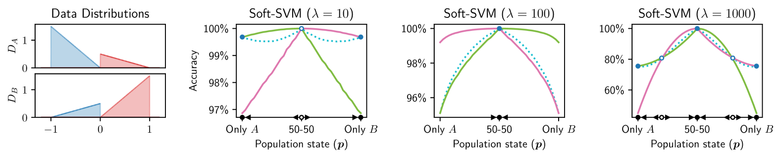
Figure 7: Varying regularization strength for Soft-SVM classifiers. (Left) Data distributions. (Center Left) Evolutionary prediction game induced by a Soft-SVM classifier with $\lambda=10$. The game has two stable equilibria at the boundaries, and an unstable coexistence equilibrium. (Center Right) Game induced by a Soft-SVM classifier with $\lambda=100$. The game has one stable coexistence equilibrium. (Right) Game induced by a Soft-SVM classifier with $\lambda=1000$. The game has five equilibria: Two stable single-group equilibria, one stable beneficial coexistence equilibrium at ${\bm{p}}=(0.5,0.5)$, and two unstable coexistence equilibria at ${\bm{p}}\approx(0.2,0.8)$ and ${\bm{p}}\approx(0.8,0.2)$.

In Figure 7, we vary the regularization strength for the distributions specified in Section B.5.1 with imbalance parameter $\alpha=0.75$. We observe that the system transition between three topologically-distinct phases: For weak regularization ($\lambda=10$), coexistence is beneficial but not stable. For intermediate regularization ($\lambda=100$), coexistence is beneficial and stable. Interestingly, for strong regularization ($\lambda=1000$), the game has five equilibria – Two stable single-group equilibria, one stable coexistence equilibia, and two unstable coexistence equilibria.

B.6 k-NN Classifiers With Label Noise

Definition B.18 (k-Nearest-Neighbors (k-NN); e.g. Shalev-Shwartz & Ben-David (2014), Section 19.1).

Let $k$ be an odd positive integer. Given a training set $S\in\left({\mathcal{X}\times\mathcal{Y}}\right)^{n}$ and a feature vector $x$, denote the $k$ nearest neighbors of $x$ in the training set by $N(x)$. The k-NN classifier returns the majority label $y$ among the members of $N(x)$.

B.6.1 Data distribution

Consider a two-group binary classification setting ($K=2$, $\mathcal{Y}={\left\{{-1,1}\right\}}$). Denote the two groups by $[K]={\left\{{A,B}\right\}}$, and let $\alpha>0$, $\beta\geq 0.5$. The data distributions for the two groups are defined symmetrically:

• Each group is comprised of a majority subgroup and a minority subgroup. The proportion of the majority subgroup is $\beta\geq 0.5$.

• One subgroup is initially contains positively-labeled data, denoted by $D_{\mathrm{pos}}\in{\Delta\left({\mathcal{X}\times{\left\{{1}\right\}}}\right)}$. Conversely, the other subgroup is initially comprised of data with negative labels, and denoted by $D_{\mathrm{neg}}\in{\Delta\left({\mathcal{X}\times{\left\{{-1}\right\}}}\right)}$. The positive subgroup is the majority of group $A$, and the negative subgroup is majority of group $B$.

• For each group, the labels in the majority subgroup are flipped with probability $\alpha$. For any data distribution $D\in{\Delta\left({{\mathcal{X}\times\mathcal{Y}}}\right)}$, we denote its noisy version by $\tilde{D}^{\alpha}$.

• It is assumed that the positive and negative data distribution have bounded support, and are sufficiently far apart such that the nearest neighbor of any sample is from the same group.

Overall we have:

$$D_{A} =\beta\tilde{D}^{\alpha}_{\mathrm{pos}}+(1-\beta)D_{\mathrm{neg}}$$

$$D_{B} =(1-\beta)D_{\mathrm{pos}}+\beta\tilde{D}^{\alpha}_{\mathrm{neg}}$$

The construction is illustrated in Figure 4 (Center).

B.6.2 Coexistence

Proposition B.19 (Convex combinations).

Let ${\bm{p}}=(1-p,p)\in{\Delta\left({{\left\{{A,B}\right\}}}\right)}$, and denote $\gamma=p-2p\beta+\beta$. It holds that:

$$D_{\bm{p}}=\gamma\tilde{D}^{\frac{\beta(1-p)}{\gamma}\alpha}_{\mathrm{pos}}+(1-\gamma)\tilde{D}^{\frac{\beta p}{1-\gamma}\alpha}_{\mathrm{neg}}$$

Proof.

For any mixture coefficient $q\in[0,1]$, the label-flipped datasets satisfy:

$$(1-q)\tilde{D}^{\alpha}+qD=\tilde{D}^{(1-q)\alpha}$$ (10)

The convex combination of the mixture coefficients of corresponding to $D_{\mathrm{pos}}$ and $\tilde{D}^{\alpha}_{\mathrm{pos}}$, is given by:

$$(1-p)\beta+p(1-\beta)=p+\beta-2p\beta=\gamma$$ (11)

Plugging Equation 11 into Equation 10, we obtain that the corresponding $q$ for the positive mixture is:

$$q_{\mathrm{pos}}=\frac{(1-p)\beta}{(1-p)\beta+p(1-\beta)}=\frac{\beta(1-p)}{\gamma}$$

and for the negative mixture:

$$q_{\mathrm{neg}}=\frac{p\beta}{p\beta+(1-p)(1-\beta)}=\frac{\beta p}{1-\gamma}$$

Combining the two equations above yields the result. ∎

Proposition B.20 (Reflection-exchange symmetry).

Let ${\bm{p}}=(1-p,p)$, and let ${\bm{p}}^{\prime}=(p,1-p)$. For the prediction setting defined above and for any classifier $h^{*}$ trained on a dataset $S\sim D^{n}_{\bm{p}}$, it holds that:

$$\mathbb{E}_{S\sim D_{{\bm{p}}}}{\left[{\mathrm{acc}_{D_{A}}(h^{*})}\right]}=\mathbb{E}_{S\sim D_{{\bm{p}}^{\prime}}}{\left[{\mathrm{acc}_{D_{B}}(h^{*})}\right]}$$

Proof.

From symmetry of the definition. Intuitively, $\mathbb{E}_{S\sim D_{{\bm{p}}}}{\left[{\mathrm{acc}_{D_{B}}(h^{*})}\right]}$ can be obtained by reflecting $\mathbb{E}_{S\sim D_{{\bm{p}}}}{\left[{\mathrm{acc}_{D_{A}}(h^{*})}\right]}$ across the ${\bm{p}}$ axis. ∎

Proposition B.21 (Expected prediction of $k$-NN).

Let $D_{x}\in{\Delta\left({\mathcal{X}}\right)}$ be a distribution over features, let $\alpha>0$ be a noise parameter, and let $k$ be an odd number greater or equal to $1$. Denote the label distribution by $D^{\alpha}_{y}=1-2\mathrm{Bernoulli}(\alpha)$, and denote the joint feature-label distribution by $D=D_{x}\otimes D_{y}^{\alpha}\in{\Delta\left({{\mathcal{X}\times\mathcal{Y}}}\right)}$. Let $h:\mathcal{X}\to{\left\{{-1,1}\right\}}$ be a $k$-Nearest-Neighbors ($k$-NN) classifier trained on a dataset $S\sim D^{n}$ with $n\geq k$, and let $x\in\mathcal{X}$. It holds that:

$$\mathbb{E}_{S\sim D^{n}}{\left[{h(x)}\right]}=-1+2\phi_{k}(\alpha)$$

Where $\phi_{k}(\alpha)$ the cumulative distribution function (CDF) of a $\mathrm{Binomial}\left(k,\alpha\right)$ random variable, taken at $\left\lfloor\frac{k}{2}\right\rfloor$:

$$\phi_{k}(\alpha)=\Pr\left(\mathrm{Binomial}\left(k,\alpha\right)\leq\left\lfloor\frac{k}{2}\right\rfloor\right)$$

Proof.

Denote the $k$-NN training set by $S\sim D^{n}$. For any $x\in\mathcal{X}$, denote its $k$ nearest neighbors by $N(x)\in\left({\mathcal{X}\times\mathcal{Y}}\right)^{n}$. Denote by $N_{\mathrm{neg}}(x)$ the number of neighbors with negative labels:

$$N_{\mathrm{neg}}(x)={\left|{{\left\{{(x^{\prime},y^{\prime})\in N(x)\mid y^{\prime}=-1}\right\}}}\right|}$$

Since features and labels in $D$ are assumed to be independent, the number of neighbors with negative labels is a binomial random variable:

$$N_{\mathrm{neg}}(x)\sim\mathrm{Binomial}\left(k,\alpha\right)$$

As a $k$-NN classifier predicts the label according to the majority label in $N(x)$, the expectation value of the label of $x$, taken over the randomness of the training set, depends on the cumulative distribution function of $N_{\mathrm{neg}}(x)$:

$$\mathbb{E}_{S\sim D^{n}}{\left[{h(x)}\right]} =-1+2\Pr\left(h(x)=1\right)$$

$$=-1+2\Pr\left(N_{\mathrm{neg}}(x)\leq\left\lfloor\frac{k}{2}\right\rfloor\right)$$

And using the definition of $\phi_{k}(\alpha)$, we obtain:

$$\mathbb{E}_{S\sim D^{n}}{\left[{h(x)}\right]}=-1+2\phi_{k}(\alpha)$$

∎

Lemma B.22 (Expected accuracy).

For the distributions $D_{A}$, $D_{B}$ defined above, let ${\bm{p}}=(1-p,p)\in{\Delta\left({{\left\{{A,B}\right\}}}\right)}$, and let $k>0$ be an odd integer. Denote by $h_{\bm{p}}$ the $k$-Nearest-Neighbor ($k$-NN) classifier trained on data sampled from $D_{\bm{p}}$. Assume that the training set contains feature vectors from both subgroups, and that the supports of the feature vector distributions in the datasets $D_{\mathrm{pos}}$, $D_{\mathrm{neg}}$ are sufficiently far apart. The expected accuracy of $h_{\bm{p}}$ with respect to $D_{A}$ is:

$$\mathbb{E}_{S\sim D_{\bm{p}}^{n}}{\left[{\mathrm{acc}_{D_{A}}(h^{*})}\right]}= \beta\left(\frac{1+(1-2\alpha)\left(-1+2\phi_{k}\left(\frac{\beta(1-p)}{\gamma}\alpha\right)\right)}{2}\right)$$ (12)

$$+(1-\beta)\left(\frac{1+(-1)\left(1-2\phi_{k}\left(\frac{\beta p}{1-\gamma}\alpha\right)\right)}{2}\right)$$

Where $\phi_{k}(\alpha)$ the cumulative distribution function of a $\mathrm{Binomial}\left(k,\alpha\right)$ variable, taken at $\left\lfloor\frac{k}{2}\right\rfloor$.

Proof.

Denote the training set by $S={\left\{{(x_{i},y_{i})}\right\}}_{i=1}^{n}\sim D_{\bm{p}}^{n}$, and denote the learned 1-NN classifier by $h_{\bm{p}}$. For any $x\in\mathcal{X}$, denote its nearest neighbor in the training set by $i^{*}(x)=\operatorname*{arg\,min}_{i\in[n]}d(x,x_{i})$. The expected accuracy of $h_{\bm{p}}$ with respect to $D_{A}$ is given by:

$$\mathbb{E}_{S\sim D_{\bm{p}}^{n}}{\left[{\mathrm{acc}_{D_{A}}(h)}\right]} =\mathbb{E}_{S\sim D_{\bm{p}}^{n},(x,y)\sim D_{A}}{\left[{\frac{1+yy_{i^{*}(x)}}{2}}\right]}$$

Since the supports of the subgroups are sufficiently far apart, the nearest neighbor $i^{*}(x)$ always originates from the same subgroup as $x$. From this we obtain that $y$ and $y_{i^{*}(x)}$ are independent given the subgroup from which $(x,y)$ was sampled ($\in{\left\{{\mathrm{pos},\mathrm{neg}}\right\}}$). Thus, for noisy data from the positive subgroup ($D^{\alpha}_{\mathrm{pos}}$), we have:

$$\mathbb{E}_{S\sim D_{\bm{p}}^{n}}{\left[{\mathrm{acc}_{\tilde{D}_{\mathrm{pos}}^{\alpha}}(h)}\right]} =\mathbb{E}_{S\sim D_{\bm{p}}^{n},(x,y)\sim\tilde{D}^{\alpha}_{\mathrm{pos}}}{\left[{\frac{1+yy_{i^{*}(x)}}{2}}\right]}$$

$$=\frac{1+\mathbb{E}{\left[{y}\right]}\mathbb{E}{\left[{y_{i^{*}(x)}}\right]}}{2}$$

$$=\frac{1+(1-2\alpha)\left(-1+2\phi_{k}\left(\frac{\beta(1-p)}{\gamma}\alpha\right)\right)}{2}$$

Where the identity $\mathbb{E}{\left[{y}\right]}=(1-2\alpha)$ is given by the definition of $\tilde{D}_{\mathrm{pos}}^{\alpha}$, the definition of $\gamma$ is given by Proposition B.19, and the identity $\mathbb{E}{\left[{y_{i^{*}(x)}}\right]}=\left(-1+2\phi_{k}\left(\frac{\beta(1-p)}{\gamma}\alpha\right)\right)$ is given by Proposition B.21.

Similarly, for clean data from the negative subgroup ($D_{\mathrm{neg}}$), we obtain:

$$\mathbb{E}_{S\sim D_{\bm{p}}^{n}}{\left[{\mathrm{acc}_{D_{\mathrm{neg}}}(h)}\right]} =\mathbb{E}_{S\sim D_{\bm{p}}^{n},(x,y)\sim D_{\mathrm{neg}}}{\left[{\frac{1+yy_{i^{*}(x)}}{2}}\right]}$$

$$=\frac{1+\mathbb{E}{\left[{y}\right]}\mathbb{E}{\left[{y_{i^{*}(x)}}\right]}}{2}$$

$$=\frac{1+(-1)\left(1-2\phi_{k}\left(\frac{\beta p}{1-\gamma}\alpha\right)\right)}{2}$$

and jointly:

$$\mathbb{E}_{S\sim D_{\bm{p}}^{n}}{\left[{\mathrm{acc}_{A}(h)}\right]}= \beta\mathbb{E}_{S\sim D_{\bm{p}}^{n}}{\left[{\mathrm{acc}_{\tilde{D}_{\mathrm{pos}}^{\alpha}}(h)}\right]}+(1-\beta)\mathbb{E}_{S\sim D_{\bm{p}}^{n}}{\left[{\mathrm{acc}_{D_{\mathrm{neg}}}(h)}\right]}$$

And finally, plugging in the expected accuracy values calculated above yields the desired result. ∎

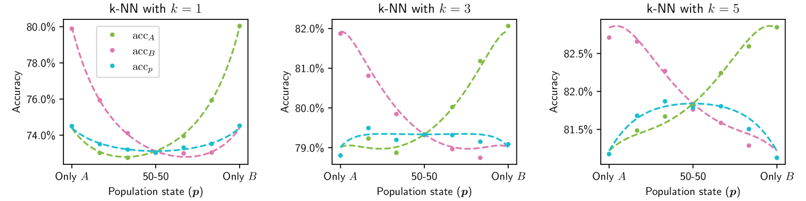
Figure 8: k-NN accuracy for the construction specified in Section B.6.1. The plots show alignment between the theoretical curves (Lemma B.22) and empirical simulations (mean accuracies represented by dots). For $k=3,5$ the game has a stable beneficial coexistence.

Proposition B.23.

For $k=1$, a prediction game induced by a $1$-NN classifier trained on dataset with label noise has the following properties:

1. A stable coexistence equilibrium exists if and only if $\alpha\in\left(0,1-\frac{1}{2\beta}\right)$. If a stable coexistence equilibrium exists, then it exists at the uniform population state ${\bm{p}}=(0.5,0.5)$.

2. The overall welfare at the coexistence state ${\bm{p}}=(0.5,0.5)$ is lower than the overall welfare at extinction states ${\bm{p}}\in{\left\{{(1,0),(0,1)}\right\}}$.

Proof.

By applying Lemma B.22. When $k=1$, the $\phi_{k}$ function satisfies:

$$\phi_{k=1}(\alpha)=\Pr\left(\mathrm{Binomial}(1,\alpha)\leq 0\right)=1-\alpha$$

Plugging into Equation 12 and using the symmetry argument in Proposition B.20, we obtain:

$$\mathrm{acc}_{A}\left(h^{*}_{{\bm{p}}=(1,0)}\right)=\mathrm{acc}_{B}\left(h^{*}_{{\bm{p}}=(0,1)}\right) =2\alpha\beta(\alpha-1)+1$$

$$\mathrm{acc}_{B}\left(h^{*}_{{\bm{p}}=(1,0)}\right)=\mathrm{acc}_{A}\left(h^{*}_{{\bm{p}}=(0,1)}\right) =1-\alpha$$

$$\mathrm{acc}_{A}\left(h^{*}_{{\bm{p}}=(0.5,0.5)}\right)=\mathrm{acc}_{B}\left(h^{*}_{{\bm{p}}=(0.5,0.5)}\right) =2\alpha\beta(\alpha\beta-1)+1$$

For (1), a stable equilibrium exists if:

$$\mathrm{acc}_{A}\left(h^{*}_{{\bm{p}}=(1,0)}\right)<\mathrm{acc}_{B}\left(h^{*}_{{\bm{p}}=(1,0)}\right)$$

Plugging in the values calculated above:

$$2\alpha\beta(\alpha-1)+1<1-\alpha$$

Which is satisfied when $\alpha\in\left(0,1-\frac{1}{2\beta}\right)$.

For (2), we note that $\beta\leq 1$, and therefore:

$$\mathrm{acc}_{A}\left(h^{*}_{{\bm{p}}=(1,0)}\right)-\mathrm{acc}_{A}\left(h^{*}_{{\bm{p}}=(0.5,0.5)}\right)=\alpha\beta(\alpha-\alpha\beta)=\alpha^{2}\beta(1-\beta)\geq 0$$

∎

Proof of Theorem 5.2.

By Proposition B.23, using e.g. $(\alpha,\beta)=(0.2,0.8)$. We observe that the conditions of the proposition are satisfied for this choice of constants, as $\alpha=0.2<0.375=1-\frac{1}{2\cdot 0.8}=1-\frac{1}{2\beta}$. ∎

B.7 Hard-SVM With Finite Data

Definition B.24 (Hard-SVM; e.g. Shalev-Shwartz & Ben-David (2014), Section 15.1).

Given a linearly-separable training set ${\left\{{(x_{i},y_{i})}\right\}}_{i=1}^{n}\in\left(\mathbb{R}^{d}\times{\left\{{-1,1}\right\}}\right)^{n}$, the Hard-SVM algorithm outputs a linear classifier $\operatorname*{sgn}(w^{*}\cdot x+b^{*})$ which maximizes the margin of the decision hyperplane:

$$(w^{*},b^{*})=\operatorname*{arg\,max}_{(w,b);\left\lVert{w}\right\rVert=1}\min_{i\in[n]}y_{i}(w\cdot x+b)$$

Remark B.25 (One-dimensional Hard-SVM).

For one dimensional data, denote by $x^{+}_{\mathrm{min}}$ the minimal $x$ with a positive label in the training set by $x^{+}_{\mathrm{min}}=\min_{i}{\left\{{x_{i}\mid y_{i}=1}\right\}}$. Similarly, denote by $x^{-}_{\mathrm{max}}$ the maximal $x$ with a negative label in the training set by $x^{-}_{\mathrm{max}}=\max_{i}{\left\{{x_{i}\mid y_{i}=-1}\right\}}$. When $x^{+}_{\mathrm{min}}\geq x^{-}_{\mathrm{max}}$, the Hard-SVM decision margin is given by:

$$x_{\mathrm{margin}}=\frac{x^{-}_{\mathrm{max}}+x^{+}_{\mathrm{min}}}{2}$$ (13)

B.7.1 Data Distribution

Let $\varepsilon>0$, and denote by $\delta(x=a)$ the Dirac delta distribution centered around $x=a$.

$$X_{A} \sim 0.5\left(\mathrm{Uniform}\left([0,1]\right)+\varepsilon\right)+0.5\delta(x=-\varepsilon)$$

$$X_{B} =-X_{A}$$

$$Y|X =\begin{cases}1&X\geq 0\\ -1&X<0\end{cases}$$

$D_{A}$ is the distribution of tuples $(X_{A},Y|X_{A})$, and $D_{B}$ is defined correspondingly as $D_{B}=(X_{B},Y|X_{B})$. The distributions are illustrated in Figure 4 (Right).

B.7.2 Coexistence

Proposition B.26.

For a given positive integer $N$, Let $n\sim\mathrm{Binomial}\left(N,\frac{1}{2}\right)$, let $x_{1},\dots,x_{n}\sim\mathrm{Uniform}\left([0,1]\right)$, and let $x_{\mathrm{min}}=\min_{i\in[n]}x_{i}$. Then for $N\geq 15$, it holds that:

$$\mathbb{E}{\left[{x_{\mathrm{min}}}\right]}\geq\frac{1}{N}$$

Proof.

Let $n\sim\mathrm{Binomial}\left(N,\frac{1}{2}\right)$. By Hoeffding’s inequality, it holds that:

$$\mathbb{P}_{n}{\left[{n-\frac{N}{2}\geq t}\right]}\leq e^{-\frac{2t^{2}}{N^{2}}}$$

And for $t=\frac{N}{4}$ we obtain:

$$\mathbb{P}_{n}{\left[{n\geq\frac{3N}{4}}\right]}\leq e^{-\frac{N}{8}}$$ (14)

For any fixed $n$, let $x_{1},\dots,x_{n}\sim\mathrm{Uniform}\left([0,1]\right)$, and denote the first order statistic among ${\left\{{x_{i}}\right\}}$ by $x_{\mathrm{min},n}=\min_{i\in[n]}x_{i}$. As each $x_{i}$ is a uniform random variable over the unit interval, the first order statistic admits a beta distribution:

$$x_{\mathrm{min},n}\sim\mathrm{Beta}(1,n)$$

and therefore:

$$\mathbb{E}{\left[{x_{\mathrm{min},n}}\right]}=\frac{1}{n+1}$$ (15)

Now consider the compound variable $x_{\mathrm{min}}=x_{\mathrm{min,n}}$ where $n\sim\mathrm{Binomial}\left(N,\frac{1}{2}\right)$. Applying the law of total expectation:

$$\mathbb{E}{\left[{x_{\mathrm{min}}}\right]} =\mathbb{E}_{n}{\left[{\mathbb{E}{\left[{x_{\mathrm{min}}\mid n}\right]}}\right]}$$

$$=\mathbb{E}_{n}{\left[{\mathbb{E}{\left[{x_{\mathrm{min,n}}}\right]}}\right]}$$

By Equation 15 we obtain the expectation of $$x_{\mathrm{min},n}$$:

$$\mathbb{E}{\left[{x_{\mathrm{min}}}\right]} =\mathbb{E}_{n}{\left[{\frac{1}{n+1}}\right]}$$

Equation 14 gives a lower bound on the expectation:

$$\mathbb{E}{\left[{x_{\mathrm{min}}}\right]} \geq\overbrace{\frac{1}{\frac{3N}{4}+1}\cdot\left(1-e^{-\frac{N}{8}}\right)}^{n<\frac{3N}{4}}+\overbrace{0\cdot e^{-\frac{N}{8}}}^{n\geq\frac{3N}{4}}$$

Then for $$N\geq 15$$ it holds that:

$$\mathbb{E}{\left[{x_{\mathrm{min}}}\right]} \geq\frac{1}{N}$$

As required.

∎

Proposition B.27.

For the distribution defined above, assume the Hard-SVM classifier is trained on dataset of size $n\geq 21$, and let $\varepsilon\in\left(0,\frac{1}{2n}\right)$. It holds that:

1. When the classifier is trained on $D_{\bm{p}}$ for ${\bm{p}}=(1,0)$:

   $$\mathbb{E}{\left[{\mathrm{acc}_{\bm{p}}(h)}\right]}=\mathbb{E}{\left[{\mathrm{acc}_{A}(h)}\right]} \leq 1-\frac{1}{8n}$$

2. When the classifier is trained on $D_{\bm{p}}$ for ${\bm{p}}=(0,1)$:

   $$\mathbb{E}{\left[{\mathrm{acc}_{\bm{p}}(h)}\right]}=\mathbb{E}{\left[{\mathrm{acc}_{B}(h)}\right]} \leq 1-\frac{1}{8n}$$

3. When the classifier is trained on $D_{\bm{p}}$ for ${\bm{p}}=(0.5,0.5)$:

   $$\mathrm{acc}_{{\bm{p}}}(h_{n})=\mathbb{E}{\left[{\mathrm{acc}_{A}(h)}\right]}=\mathbb{E}{\left[{\mathrm{acc}_{B}(h)}\right]}\geq 1-2\left(1-\frac{1}{4}\right)^{n}$$

4. Coexistence is beneficial.

Proof.

For case (1), the Hard-SVM algorithm trains on data sampled from $D_{A}$. Denote the size of the dataset by $n$ and the corresponding Hard-SVM classfier by $h_{n}$. We note that $h_{n}$ is a random variable depending on the dataset. For a dataset ${\left\{{(x_{i},y_{i})}\right\}}_{i=1}^{n}\sim D_{A}^{n}$, Since the problem is one-dimensional, the Hard-SVM decision margin is given by Equation 13:

$$x_{\mathrm{margin}}=\frac{x^{-}_{\mathrm{max}}+x^{+}_{\mathrm{min}}}{2}=\frac{x^{+}_{\mathrm{min}}-\varepsilon}{2}>0$$

And the expected accuracy of each group is given by:

$$\mathbb{E}{\left[{\mathrm{acc}_{A}(h_{n})\mid\omega^{c}}\right]} =\frac{1}{2}+\frac{1}{2}\left(1-x_{\mathrm{margin}}+\varepsilon\right)=1-\frac{x^{+}_{\mathrm{min}}-\varepsilon}{4}+\frac{\varepsilon}{4}$$

By Proposition B.26 and for $n\geq 15$, it holds that $\mathbb{E}{\left[{x_{\mathrm{margin}}}\right]}\geq\frac{1}{n}+\varepsilon$, and therefore:

$$\mathbb{E}{\left[{\mathrm{acc}_{A}(h_{n})\mid\omega^{c}}\right]} \leq 1-\frac{1}{4n}+\frac{1}{8n}=1-\frac{1}{8n}$$

Case (2) follows from symmetry.

For case (3), denote by $\omega$ the bad event in which the training set ${\left\{{(x_{i},y_{i})}\right\}}_{i=1}^{n}\sim D_{\bm{p}}^{n}$ does not contain $x_{i}\in{\left\{{-\varepsilon,\varepsilon}\right\}}$. By the union bound, the probability of this event is bounded by $2\left(1-\frac{1}{4}\right)^{n}$, and therefore the accuracy for ${\bm{p}}=(0.5,0.5)$ is bounded from below by:

$$\mathrm{acc}_{{\bm{p}}}(h_{n})\geq 1-2\left(1-\frac{1}{4}\right)^{n}$$

Finally, for (4), we note that $1-2\left(1-\frac{1}{4}\right)^{n}\geq 1-\frac{1}{8n}$ for all $n\geq 21$. ∎

Proof of Theorem 5.3.

By Proposition B.27. ∎

B.8 Stabilizing Coexistence

Proof of Proposition 5.4.

Let $F({\bm{p}})$ be an evolutionary prediction game induced by an optimal learning algorithm $\mathcal{A}({\bm{p}})$, and let ${\bm{p}}^{*}$ be an unstable coexistence equilibrium with full support (${\left|{\operatorname*{support}({\bm{p}}^{*})}\right|}=K$). The game induced by $\mathcal{A}^{\prime}({\bm{p}})$ in the neighborhood of ${\bm{p}}^{*}$ is $F^{\prime}({\bm{p}})=F(2{\bm{p}}^{*}-{\bm{p}})$. By Lemma B.14, the game $F({\bm{p}})$ is a potential game, and therefore admits a potential function $f({\bm{p}})=\mathrm{acc}_{\bm{p}}(h_{\bm{p}})$. Consider the potential function $f^{\prime}({\bm{p}})=-f(2{\bm{p}}^{*}-{\bm{p}})$. By the chain rule, it holds that:

$$\nabla f^{\prime}({\bm{p}})=-(\nabla f)(2{\bm{p}}^{*}-{\bm{p}})\cdot\nabla(2{\bm{p}}^{*}-{\bm{p}})=F(2{\bm{p}}^{*}-{\bm{p}})=F^{\prime}({\bm{p}})$$

And therefore $f^{\prime}({\bm{p}})$ is a potential function for the game $F^{\prime}({\bm{p}})$ in the neighborhood of ${\bm{p}}^{*}$. The equilibrium ${\bm{p}}^{*}$ is unstable, and therefore by (Sandholm, 2010, Theorem 8.2.1) it is not a maximizer of $f({\bm{p}})$. Moreover, by Proposition B.9 the potential function $f({\bm{p}})=\mathrm{acc}_{\bm{p}}(h_{\bm{p}})$ is convex, and as ${\bm{p}}^{*}$ is assumed to have full support, it is also a global minimizer of $f({\bm{p}})$. From this we conclude that ${\bm{p}}^{*}$ is a global maximizer of $f^{\prime}({\bm{p}})$, and therefore the equilibrium ${\bm{p}}^{*}$ is stable under the evolutionary game induced by $\mathcal{A}^{\prime}$. ∎

Appendix C Experimental Details

Code.

We implement our analysis in Python. Our synthetic-data experiments rely on scikit-learn for learning algorithm implementations (Pedregosa et al., 2011), and our real-data experiments rely on PyTorch (Paszke et al., 2019) and ffcv (Leclerc et al., 2023). Code is available at: https://github.com/edensaig/evolutionary-prediction-games.

Hardware.

Synthetic data simulations were run on a single Macbook Pro laptop, with 16GB of RAM, M2 processor, and no GPU support. Experiments involving neural networks (Section 6) were run on a dedicated server with an AMD EPYC 7502 CPU, 503GB of RAM, and an Nvidia RTX A4000 GPU.

Evolutionary dynamics.

For simulation of evolutionary dynamics (Figure 3, Figure 5), we use the discrete replicator equation given by (Taylor & Jonker, 1978, Equation (3)).

Architectures.

For CIFAR-10, we use the Resnet-9 architecture and training code provided in the CIFAR-10 example code in the ffcv Github repository (libffcv/ffcv, commit 7885f40), with modifications to control the probability of horizontal flips in training and testing. For MNIST, we use the convolutional neural network provided in the MNIST example code in the PyTorch examples Github repository (pytorch/examples, commit 37a1866). The MNIST network has two convolutional layers, and two fully-connected layers, with dropout and max pooling. Training is performed for 200 epochs using SGD with learning rate $0.01$ and momentum $0.5$. We use ffcv for data loading in both experiments.

Runtime.

A single run of the complete synthetic data pipeline takes roughly 20 minutes on a laptop. A single repetition of each real-data experiment (i.e. sampling $h\sim\mathcal{A}({\bm{p}})$ and computing marginal accuracies) takes roughly 10 minutes.

References

- Bisin & Verdier (2001) Bisin, A. and Verdier, T. The economics of cultural transmission and the dynamics of preferences. Journal of Economic theory, 97(2):298–319, 2001.
- Brown et al. (2022) Brown, G., Hod, S., and Kalemaj, I. Performative prediction in a stateful world. In International conference on artificial intelligence and statistics, pp. 6045–6061. PMLR, 2022.
- Chesson (2000) Chesson, P. Mechanisms of maintenance of species diversity. Annual review of Ecology and Systematics, 31(1):343–366, 2000.
- Conger et al. (2024) Conger, L., Hoffmann, F., Mazumdar, E., and Ratliff, L. Strategic distribution shift of interacting agents via coupled gradient flows. Advances in Neural Information Processing Systems, 36, 2024.
- D’Amour et al. (2020) D’Amour, A., Srinivasan, H., Atwood, J., Baljekar, P., Sculley, D., and Halpern, Y. Fairness is not static: deeper understanding of long term fairness via simulation studies. In Proceedings of the 2020 Conference on Fairness, Accountability, and Transparency, pp. 525–534, 2020.
- Hardin (1960) Hardin, G. The competitive exclusion principle: an idea that took a century to be born has implications in ecology, economics, and genetics. science, 131(3409):1292–1297, 1960.
- Hashimoto et al. (2018) Hashimoto, T., Srivastava, M., Namkoong, H., and Liang, P. Fairness without demographics in repeated loss minimization. In International Conference on Machine Learning, pp. 1929–1938. PMLR, 2018.
- He et al. (2016) He, K., Zhang, X., Ren, S., and Sun, J. Deep residual learning for image recognition. In Proceedings of the IEEE conference on computer vision and pattern recognition, pp. 770–778, 2016.
- Hofbauer & Sigmund (1998) Hofbauer, J. and Sigmund, K. Evolutionary games and population dynamics. Cambridge university press, 1998.
- Kleinberg et al. (2009) Kleinberg, R., Piliouras, G., and Tardos, É. Multiplicative updates outperform generic no-regret learning in congestion games. In Proceedings of the forty-first annual ACM symposium on Theory of computing, pp. 533–542, 2009.
- Kleinberg et al. (2011) Kleinberg, R. D., Ligett, K., Piliouras, G., and Tardos, É. Beyond the nash equilibrium barrier. In ICS, volume 20, pp. 125–140, 2011.
- Krizhevsky (2009) Krizhevsky, A. Learning multiple layers of features from tiny images. Master’s thesis, University of Toronto, 2009.
- Leclerc et al. (2023) Leclerc, G., Ilyas, A., Engstrom, L., Park, S. M., Salman, H., and Madry, A. FFCV: Accelerating training by removing data bottlenecks. In Computer Vision and Pattern Recognition (CVPR), 2023.
- LeCun (1998) LeCun, Y. The mnist database of handwritten digits. http://yann. lecun. com/exdb/mnist/, 1998.
- Liu et al. (2018) Liu, L. T., Dean, S., Rolf, E., Simchowitz, M., and Hardt, M. Delayed impact of fair machine learning. In International Conference on Machine Learning, pp. 3150–3158. PMLR, 2018.
- Maynard Smith & Price (1973) Maynard Smith, J. and Price, G. R. The logic of animal conflict. Nature, 246(5427):15–18, 1973.
- Moran (1958) Moran, P. A. P. Random processes in genetics. In Mathematical proceedings of the cambridge philosophical society, volume 54, pp. 60–71. Cambridge University Press, 1958.
- Paszke et al. (2019) Paszke, A., Gross, S., Massa, F., Lerer, A., Bradbury, J., Chanan, G., Killeen, T., Lin, Z., Gimelshein, N., Antiga, L., et al. Pytorch: An imperative style, high-performance deep learning library. Advances in neural information processing systems, 32, 2019.
- Pedregosa et al. (2011) Pedregosa, F., Varoquaux, G., Gramfort, A., Michel, V., Thirion, B., Grisel, O., Blondel, M., Prettenhofer, P., Weiss, R., Dubourg, V., Vanderplas, J., Passos, A., Cournapeau, D., Brucher, M., Perrot, M., and Duchesnay, E. Scikit-learn: Machine learning in Python. Journal of Machine Learning Research, 12:2825–2830, 2011.
- Perdomo et al. (2020) Perdomo, J., Zrnic, T., Mendler-Dünner, C., and Hardt, M. Performative prediction. In International Conference on Machine Learning, pp. 7599–7609. PMLR, 2020.
- Rockafellar (1970) Rockafellar, R. T. Convex Analysis. Princeton University Press, Princeton, 1970. ISBN 9781400873173. doi: doi:10.1515/9781400873173. URL https://doi.org/10.1515/9781400873173.
- Sandholm (2001) Sandholm, W. H. Potential games with continuous player sets. Journal of Economic theory, 97(1):81–108, 2001.
- Sandholm (2010) Sandholm, W. H. Population games and evolutionary dynamics. MIT press, 2010.
- Scholl et al. (2021) Scholl, M. P., Calinescu, A., and Farmer, J. D. How market ecology explains market malfunction. Proceedings of the National Academy of Sciences, 118(26):e2015574118, 2021.
- Shalev-Shwartz & Ben-David (2014) Shalev-Shwartz, S. and Ben-David, S. Understanding machine learning: From theory to algorithms. Cambridge university press, 2014.
- Taylor & Jonker (1978) Taylor, P. D. and Jonker, L. B. Evolutionary stable strategies and game dynamics. Mathematical biosciences, 40(1-2):145–156, 1978.
- Traulsen et al. (2006) Traulsen, A., Claussen, J. C., and Hauert, C. Coevolutionary dynamics in large, but finite populations. Physical Review E, 74(1):011901, 2006.
- Vardi (2023) Vardi, G. On the implicit bias in deep-learning algorithms. Communications of the ACM, 66(6):86–93, 2023.
- Verma & Rubin (2018) Verma, S. and Rubin, J. Fairness definitions explained. In Proceedings of the international workshop on software fairness, pp. 1–7, 2018.
- Yang et al. (2023) Yang, Y., Zhang, H., Katabi, D., and Ghassemi, M. Change is hard: A closer look at subpopulation shift. arXiv preprint arXiv:2302.12254, 2023.
- Zhang et al. (2021) Zhang, C., Bengio, S., Hardt, M., Recht, B., and Vinyals, O. Understanding deep learning (still) requires rethinking generalization. Communications of the ACM, 64(3):107–115, 2021.