Dependence of Krylov complexity on the initial operator and state

Abstract

Krylov complexity, a quantum complexity measure which uniquely characterizes the spread of a quantum state or an operator, has recently been studied in the context of quantum chaos. However, the definitiveness of this measure as a chaos quantifier is in question in light of its strong dependence on the initial condition. This article clarifies the connection between the Krylov complexity dynamics and the initial operator or state. We find that the Krylov complexity depends monotonically on the inverse participation ratio (IPR) of the initial condition in the eigenbasis of the Hamiltonian. We explain the reversal of the complexity saturation levels observed in Phys.Rev.E.107,024217, 2023 using the initial spread of the operator in the Hamiltonian eigenbasis. IPR dependence is present even in the fully chaotic regime, where popular quantifiers of chaos, such as out-of-time-ordered correlators and entanglement generation, show similar behavior regardless of the initial condition. Krylov complexity averaged over many initial conditions still does not characterize chaos.

How an isolated quantum system thermalizes is closely connected to the scrambling of an initially localized, far-from-equilibrium quantum state. As the quantum state scrambles, one expects it to become more complex in an intuitive sense. However, when trying to quantify this complexity rigorously, one soon encounters a problem: the ambiguity of the basis. For example, the complexity of a computer circuit would depend on the fixed set of gates available. Things look rather grim for a quantum state as the number of basis sets is infinite. Once a basis is fixed, the spread complexity can be defined as a function of the state’s amplitude in the orthogonal basis directions, capturing the extent of the state. Krylov basis provides a unique solution to the ambiguity by minimizing the spread complexity over all the possible bases [1]. Krylov complexity maps the complexity of a quantum state to the average position of a particle hopping on a one-dimensional chain, with the probability of hopping determined by Lanczos coefficients.

Since the spreading of quantum information in the system is a key feature of quantum chaos, Krylov complexity seems to be a suitable candidate for quantifying chaos in such systems. Similar to the other popular quantum chaos measures such as out-of-time-ordered correlator (OTOC) and entanglement generation, Krylov complexity also displays a ramp followed by saturation. The complexity growth rate is exponential in chaotic systems and the Krylov exponent upper bounds the Lyapunov exponent [2, 3]. Studies showed that the late-time saturation value of Krylov complexity carries signatures of chaos [4, 5, 6, 7]. Integrable systems tend to saturate at lower complexity values compared to nonintegrable systems. The difference in saturation is attributable to the difference in the variance of the Lanczos coefficients [4, 5, 8, 6, 7].

However, the legitimacy of Krylov complexity as a measure of quantum chaos has recently been questioned. The saturation value of the operator complexity can be completely changed by choosing a different initial operator or state [9, 10]. The authors in [9] also found that the variance of the Lanczos coefficients, although somewhat correlated with chaos, shows large fluctuations. Another study in conformal field theory models [11] pointed out that the Krylov complexity can increase exponentially even when the system remains noninteracting. Furthermore, the Krylov exponent keeps increasing monotonically in systems where the Lyapunov exponent is non-monotonic [12], prompting the authors to conjecture that the Krylov complexity works more as an entropy and less as a measure of chaos.

This conflict in the literature raises the question: What constitutes a good initial operator (or a state) for the Krylov complexity study if there is one at all? Using traceless operators as suggested in [4] does not always work, as the counter-example in [9] points out. In a paper [10] that describes discrepancies in state complexity, the authors recommend not so delocalized initial states in the energy eigenbasis for better results. If we have to scrabble around to find suitable operators and states so that Krylov complexity behaves as expected, can it even be trusted to diagnose chaos? The key to unlocking this problem is to understand how Krylov complexity depends on the initial condition. Based on the initial spread in the Hamiltonian eigenbasis, we find a surprisingly simple relationship between the complexity dynamics and the initial operators and states.

This article studies Krylov complexity of both states and operators in time-independent and periodically driven Floquet systems. For generality, we study a random matrix model for the unitary evolution of two coupled systems, with a transition to chaos depending on the coupling strength. After establishing the relation between complexity and IPR in this model, we probe well-studied physical systems, such as the quantum kicked top and transverse field Ising model, where we illuminate the contrast between Krylov complexity and other well-accepted measures of chaos in these models. In the end, we investigate whether Krylov complexity can still be used to quantify chaos despite its excessive dependence on the initial state. Since we deal with both states and operators in this paper, Krylov complexity may refer to either of them and will be made clear from the context.

Krylov complexity: Given a Hamiltonian $H$ of dimension $d$, a Hermitian operator $\mathcal{O}$, and the Liouvillian superoperator $\mathcal{L}=\commutator{H}{\cdot}$, the Krylov subspace is defined as the minimum subspace of $\mathcal{L}$ that contains $\mathcal{O}(t)$ at all times, that is, $\mathcal{K}=\{|\mathcal{O}),\,\mathcal{L}|\mathcal{O}),\,\mathcal{L}^{2}|\mathcal{O}),\dots\}$, where $|\mathcal{O})$ is the state representation of $\mathcal{O}$ in the Hilbert space of the operator. Using the Lanczos or Arnoldi iteration method, the set $\mathcal{K}$ can be orthogonalized to obtain the Krylov basis vectors $\{|K_{n})\}_{n=1}^{d_{\mathcal{K}}},$ where $d_{\mathcal{K}}$ denote the dimension of the Krylov subspace. In this paper, we use the Arnoldi method for numerical simulations. The Krylov complexity of $\mathcal{O}(t)$ is defined as

$$K_{\mathcal{C}}(t)=\sum_{n=0}^{d_{k}-1}n\left|({K_{n}}|{\mathcal{O}(t)})\right|^{2}.$$ (1)

A similar definition follows for the state complexity by simply replacing the operator $\mathcal{O}$ by a state $\ket{\psi}$. The extension of the definition to include periodically driven systems can be found in [13, 6], and also in the supplementary file.

Inverse Participation Ratio for states and operators Let the Hamiltonian $H$ or the Floquet $\mathcal{U}$ for a periodically driven system has eigenvectors $\{|v_{i}\rangle\}_{i=1}^{d}$. For an initial state $|\psi\rangle$, the IPR with respect to this eigenbasis is:

$$\mathrm{IPR}_{\mathcal{U}}(|\psi\rangle)=\sum_{i=1}^{d}|\langle v_{i}|\psi\rangle|^{4},$$ (2)

IPR varies between $\frac{1}{d}$ and one, equal to one when $\ket{\psi}$ is an eigenstate of the Floquet, and $\frac{1}{d}$ when $\ket{\psi}$ is perfectly delocalized in $\{|v_{i}\rangle\}.$

Similarly, we define IPR for an operator $\mathcal{O}.$ To treat all operators on the same footing, first, we normalize $\mathcal{O}$ by defining $\mathcal{O}=\mathcal{O}/\mathrm{Tr}\sqrt{\mathcal{O}\mathcal{O}^{\dagger}}.$ Expanding $\mathcal{O}$ in the energy eigenbasis obtained above, we get $\mathcal{O}=\sum_{i,j=1}^{d}\bra{v_{i}}\mathcal{O}|v_{j}\rangle\ket{v_{i}}\bra{v_{j}}.$ We define the IPR of $\mathcal{O}$ using the diagonal elements in this representation as follows:

$$\mathrm{IPR}_{H}(\mathcal{O})=\sum_{i=1}^{d}{|\bra{v_{i}}\mathcal{O}\ket{v_{i}}|^{2}}.$$ (3)

Equation (3) is a function of the operator’s projections along the energy eigenvectors of the dynamics. It quantifies the initial overlap and the spread of $\mathcal{O}$ along the eigenvector directions. One must note that $\sum_{i=1}^{d}|\bra{v_{i}}\mathcal{O}\ket{v_{i}}|\neq 1,$ unlike the case of states. $\mathcal{O}$ could as well be a hollow matrix in this representation, with diagonal entries all zero if $\mathcal{O}$ has zero overlap with the one-dimensional projectors along $\{\ket{v_{i}}\}.$

Krylov state complexity with random matrix transition ensemble dynamics: To examine $K_{\mathcal{C}}(t)$ in the context of quantum chaos, we choose a dynamics that transitions from regular to chaotic as a function of a parameter. To be independent of any particular model system, we consider a random matrix model of interacting bipartite systems with Floquet dynamics over one period of the form (also known as the Random matrix transition ensemble (RMTE) [14]),

$$\mathcal{U}_{\epsilon}=U_{12}(\epsilon)(U_{1}\otimes U_{2}).$$ (4)

Here, the unitaries $U_{1}$ and $U_{2}$ are chosen from the circular unitary ensemble (CUE), and they act on the Hilbert spaces of subsystem-1 and subsystem-2 respectively, each of dimension $d$. The parameter $\epsilon$ governs the strength of the interaction between the two subsystems in $U_{12}(\epsilon).$ The coupling unitary is diagonal, with the non-zero elements being $\mathrm{exp}(i2\pi\epsilon\mathscr{\xi}_{n_{1}n_{2}})$, where $1\leq n_{1},n_{2}\leq d,$ and $\xi_{n_{1}n_{2}}\in[-\frac{1}{2},\frac{1}{2})$, chosen uniformly at random. At $\epsilon=0,$ the two subsystems are non-interacting. As $\epsilon$ increases from zero to one, the eigenphase spacing distribution of the unitary matrix transitions from Poissonian to Wigner-Dyson statistics.

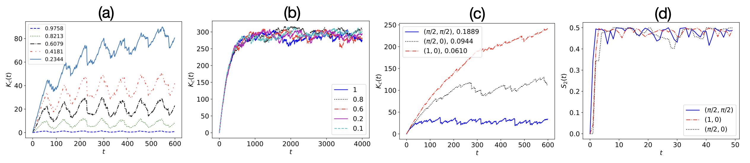
Figure 1: (a) Krylov complexity as a function of time for initial states with different IPR in the eigenbasis of $\mathcal{U}_{\epsilon=1}$. The dimensions of the subspaces are chosen to be $d=5.$ There is a monotonic relationship between the IPR of the state and the rate of growth and saturation of the complexity. (b) Krylov complexity for the states with the same IPR under different RMTE dynamics. Legends denote the $\epsilon$ values of $\mathcal{U}_{\epsilon}$. (c) Krylov complexity evolution under the kicked top unitary for three spin coherent states with $(\theta,\phi)$ values given in the parenthesis. The numeral outside the parenthesis in the legend is the IPR. The kicking strength $\kappa=6,$ and $j=15.$ (d) Linear entropy evolution for the coherent initial states in (c) under the same unitary dynamics.

First, we fix the evolution given by Eq. (4), by letting $d=5$, and choosing an $\epsilon.$ Let us consider $\epsilon=1$ so that the evolution is chaotic and the evolution unitary is denoted by $\mathcal{U}_{\epsilon=1}.$ The set of random numbers $\{\mathscr{\xi}_{n_{1}n_{2}}\}$ once generated, is fixed for the entire experiment.

The next step is to pick initial states as inputs to the Floquet evolution. We choose states with different IPRs in the eigenbasis of $\mathcal{U}_{\epsilon=1}.$ To obtain such states, we rotate $\ket{v_{1}}$, an eigenvector of $\mathcal{U}_{\epsilon=1}$ using a unitary rotation operator

$$R(\theta,\phi)=\exp[i\theta(j_{x}\mathrm{sin}(\phi)-j_{y}\mathrm{cos}(\phi))]$$ (5)

for different $(\theta,\phi).$ Here $j_{x}$ and $j_{y}$ are angular momentum operators acting in the collective Hilbert space of $\mathcal{U}_{\epsilon=1}.$ The $K_{\mathcal{C}}(t)$ for states with different IPRs is shown in Fig. 1(a). Note that the system is in the chaotic limit, yet the saturation of $K_{\mathcal{C}}(t)$ depends on the IPR of the initial state. If the state has $\mathrm{IPR}=1,$ it does not evolve, and the Krylov complexity remains zero. The more spread the initial state is in $\{|v_{i}\rangle\}$, the higher the growth rate and saturation of its complexity. Even when the number of Krylov basis vectors is the same for two states, their complexity could differ based on how the states spread within the Krylov space.

Now that the behavior of the states with different IPR under a chosen dynamics is clear, we probe the converse situation. We now vary $\epsilon$ so that the dynamics determined by $\mathcal{U}_{\epsilon}$ can be different. But we fix the initial state to be the maximally delocalized state for all $\mathcal{U}_{\epsilon}$ so that the IPR are the same. More explicitly, when subsystems are of $d=5,$ the initial state is given by the equal superposition of all the eigenstates: $\ket{\psi_{0}}=\frac{1}{\sqrt{(}25)}(\ket{v_{1}}+\ket{v_{2}}+...\ket{v_{25}}).$ Here the $\{\ket{v_{i}}\}$ vary depending on the $\mathcal{U_{\epsilon}},$ but the IPR is the same and is equal to $0.04$ regardless of $\epsilon.$ We find that the $K_{\mathcal{C}}(t)$, irrespective of the $\epsilon$ rise and saturate very close to each other, as shown in Fig.1(b). Since there are fluctuations post-saturation, we plot a long-time evolution for clarity. We also studied other states more localized in $\{\ket{v_{i}}\}$, maintaining the same IPR. Their behavior was the same. Figure 1(b) is a clear indication that the Krylov complexity is independent of the nature of the dynamics and only depends on the IPR.

Krylov state complexity with the quantum kicked top: Turning to a physical system that is well studied in the context of quantum chaos, we find that Krylov complexity can be a misleading measure of chaos. The quantum kicked top is a periodically driven system, with the evolution for one period given by the unitary [15, 16]

$$U=\exp(-i\frac{\kappa}{2j}J_{z}^{2})\exp(-i\alpha J_{y}).$$ (6)

Here $\kappa$ is the kick strength, determining the amount of chaos in the system. $\alpha$ is the angle of precession about $y$-axis, which we fix to be $\pi/2,$ and $j$ is the spin angular momentum.

To study $K_{\mathcal{C}}(t),$ we choose $j=15,$ and $\kappa=6.$ At this $\kappa,$ chaos dominates the corresponding classical phase space [15]. The evolution of the complexity for three different initial spin coherent states is shown in Fig. 1(c), again revealing the monotonic dependence on IPR. It should be noted that we are witnessing IPR dependence even in this chaotic regime.

On the other hand, studying the entanglement dynamics of the kicked top considered as a compound system of spins [17] shows a contrasting picture. The linear entropy $S_{2}(t)$ of a single spin with the rest increases and rapidly saturates close to the maximum entropy of $0.5,$ at $\kappa=6.$ The linear entropy is defined as $S_{2}(t)=1-\mathrm{Tr}\rho_{s}^{2}(t),$ where $\rho_{s}(t)$ is the reduced density matrix of a single spin. The $S_{2}(t)$ evolution is shown in Fig. 1(d). The initial states are the same as in Fig. 1(c); however, it is now impossible to differentiate one initial state from the other based on evolution. This behavior is not limited to the chosen coherent states. Randomly choosing $(\theta,\phi)$ values also gives similar growth and saturation, as expected from an underlying chaotic phase space.

Krylov operator complexity with random matrix transition ensemble dynamics: We first study the IPR dependence of the operator complexity for the random matrix evolution in Eq. (4). We fix $\epsilon=1$ as in the case of states so that we have a chaotic evolution governed by $\mathcal{U}_{\epsilon=1}$. To generate initial operators with different IPR, we rotate $\mathcal{U}_{1}$ using the rotation operator $R(\theta,\phi)$ in Eq. (5) by varying $(\theta,\phi).$ The resultant dynamics of these operators under $\mathcal{U}_{1}$ is shown in Fig. 5(a). The figure displays the dependence of the Krylov complexity on the IPR of the initial operator.

Krylov operator complexity with the quantum kicked top: We illustrate another example of $K_{\mathcal{C}}(t)$ not capturing chaos and instead following the IPR in the quantum kicked top with $j=15$ and $\kappa=6.$ Figure 5(b) shows the complexity evolution under Eq. (6) with angular momentum operators $(j_{x},j_{y},j_{z})$ as initializations. The figure shows that in the chaotic regime, the evolutions of $j_{x}$ and $j_{z}$ are identical and differ from $j_{y}$. This is in line with the IPR of these operators. Both $j_{x}$ and $j_{z}$ are hollow matrices in the energy eigenbasis and have vanishing IPR according to Eq. (3). Krylov complexity evolution of both these operators is therefore identical as seen in Fig. 5(b). $j_{y}$ has nonzero IPR (0.009), and hence lower complexity.

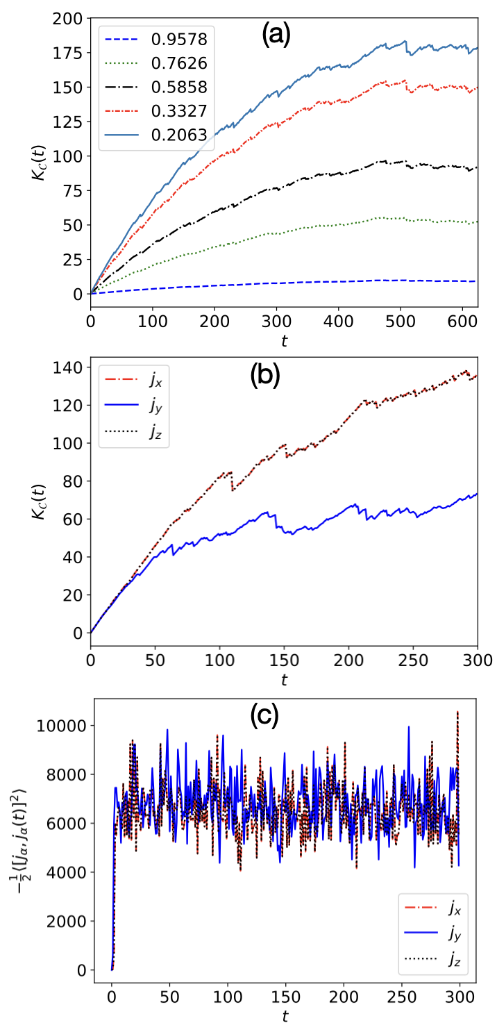
Figure 2: (a) Operator complexity for initial operators with different IPR in the eigenbasis of $\mathcal{U}_{\epsilon=1}$ of the RMTE. (b) Complexity evolution of spin operators under kicked top unitary with $j=15$ and $\kappa=6.$ Krylov complexity of $j_{x}$ and $j_{z}$ are the same, whereas that of $j_{y}$ is lower. The corresponding IPRs obtained are $j_{x}=j_{z}=0$, $j_{y}=0.009$. An inverse correlation between IPR and Krylov complexity is evident from the figure. (c) OTOC of the form $-\frac{1}{2}\langle[j_{\alpha},j_{\alpha}(t)]^{2}\rangle$, where $\alpha\in\{x,y,z\}$ show that OTOC cannot distinguish these operators. OTOC expectation value is taken with respect to the maximally mixed state, also called infinite temperature OTOC.

However, OTOC evolution of the form $-\frac{1}{2}\langle[j_{\alpha},j_{\alpha}(t)]^{2}\rangle$, where $\alpha\in\{x,y,z\}$ cannot resolve between these operators, as Fig. 5(c) shows. In a fully chaotic regime, OTOC and entanglement dynamics do not depend on the initial condition, as true chaos measures should. With the phase space lacking regular structures, one point is no different from another. However, Krylov complexity, even in the chaotic regime, shows different evolutions based on the IPR, which indicates a serious flaw for it to be a chaos measure.

Krylov operator complexity with transverse field Ising model: The authors in [9], working with a transverse field Ising model, found that the saturation level of the Krylov complexity changes based on the initial operator. The Ising Hamiltonian has nearest-neighbour coupling and a transverse magnetic field in the $X-Z$ plain, given by:

$$H=\sum_{k=1}^{L}(h_{x}\sigma_{k}^{x}+h_{z}\sigma_{k}^{z})-J\sum_{k=1}^{L-1}\sigma_{k}^{z}\sigma_{k+1}^{z}.$$ (7)

Here, $L$ is the chain length, $J$ is the interaction strength and $h_{x}$ and $h_{z}$ denote the components of the magnetic field. The operators $\sigma_{k}^{\alpha},$ where $\alpha\in\{x,y,z\}$ are local Pauli operators. Fixing $J=h_{x}=1$, the system transitions progressively from integrability to chaos as $h_{z}$ decreases from $2.5$ to $0.2.$

A stark display of the effect of the initial condition on Krylov complexity is obtained by choosing $S_{z}=\sum_{k=1}^{L}\sigma_{k}^{z}$ and $S_{x}=\sum_{k=1}^{L}\sigma_{k}^{x}$ as initial operators. The system has a reflection symmetry about the center of the chain, and the operators $S_{x}$ and $S_{z}$ lie in the positive parity sector. Working in the corresponding symmetry subspace, the complexity for $S_{z}$ evolves and saturates at a higher value in the chaotic regime compared to the regular region (see [9] or supplementary for the figure). This behavior is in line with the findings in [4, 5], and is consistent with what one would expect from studying other measures of chaos. The initial choice of $S_{x}=\sum_{k=1}^{L}\sigma_{k}^{x}$ makes the Krylov complexity behave in a way opposite to this expectation, and now there is more complexity in the integrable regime (see [9] or supplementary for the figure)!

We can explain this behavior using the spread of the initial operator in the eigenbasis of the transverse field Ising Hamiltonian. The IPR for the operators $S_{x}$ and $S_{z}$ according to Eq. (3) is shown in the table below. In each row, the operator with the smaller IPR consistently shows a higher saturation value of complexity.

$h_{z}$	IPR for $S_{x}$	IPR for $S_{z}$
0.2	$0.3545$	$0.0946$
1.35	$0.2307$	$0.3391$
2.5	$0.1351$	$0.4409$

Average Krylov complexity: Given the dependence on the initial condition, $K_{\mathcal{C}}(t)$ cannot be trusted with characterizing chaos with a single initial operator/state. However, can it at least roughly estimate chaos? In other words, can Krylov complexity saturation, averaged over many initial conditions work as a measure of chaos?

We study the transverse field Ising model in Eq. (14), averaging over one hundred initial operators in the positive parity subspace.

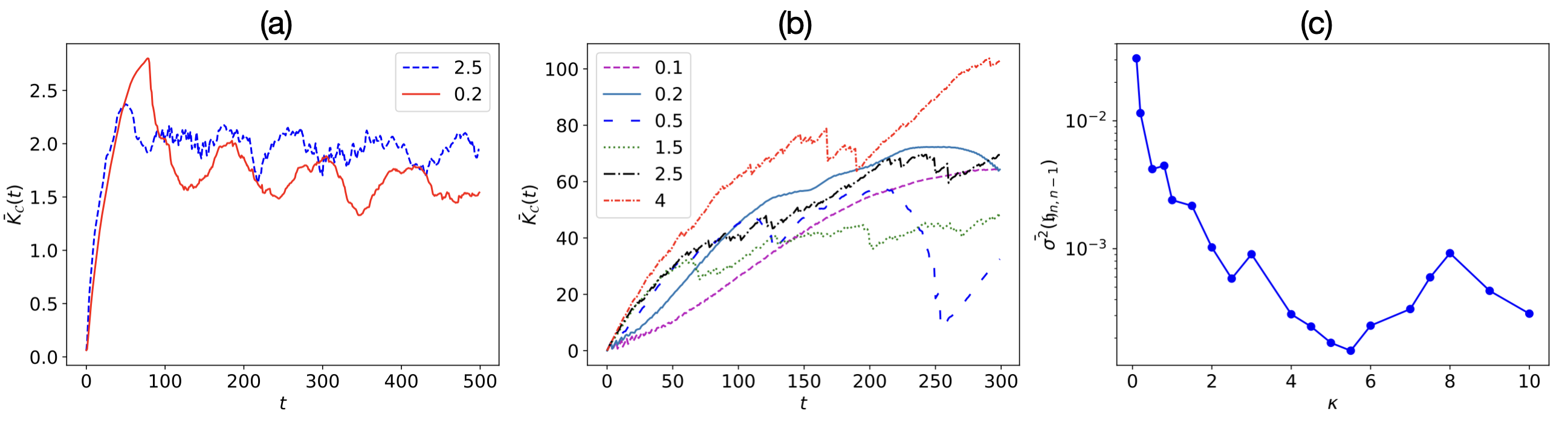
Figure 3: (a) Average Krylov complexity $\bar{K}_{\mathcal{C}}(t)$ for the transverse Ising model with $L=6$ over 100 initial operators, as mentioned in the main text. (b) $\bar{K}_{\mathcal{C}}(t)$ averaged over 100 randomly chosen initial coherent states under kicked top evolution with $j=10$ for different kick strengths $\kappa.$ (c) Variance of Arnoldi coefficients $\mathfrak{h}_{n,n-1}$ against kicking strength obtained after averaging over 100 initial coherent state evolutions using kicked top with $j=10$.

To generate the initial operators, we rotate each spin -$\frac{1}{2}$ sites in $S_{x}=\sum_{k=1}^{L}\sigma_{k}^{x}$ using the rotation operator $R(\theta,\phi)=\exp[i\theta(\sigma_{x}\mathrm{sin}(\phi)-\sigma_{y}\mathrm{cos}(\phi))]$ for $(\theta,\phi)$ chosen uniformly at random, such that $\theta\in[0,\pi)$ and $\phi\in[0,2\pi)$. We plot the average Krylov complexity (denoted $\bar{K}_{\mathcal{C}}(t)$) for $h_{z}=0.2$ corresponding to the chaotic regime, and $h_{z}=2.5$ in the regular regime, in Fig. 3(a). Other parameters of the model are kept the same as before, namely $L=6,\>\&\>J=h_{x}=1.$ Complexity at $h_{z}=0.2$ does not saturate above that of $h_{z}=2.5,$ even with the averaging. Therefore, Krylov complexity does not describe chaos even as a coarse measure.

Similarly, $\bar{K}_{\mathcal{C}}(t)$ for one hundred spin coherent states evolved with the kicked top Floquet is shown in Fig 3 (b). There is no monotonic correlation between the growth, complexity saturation, and the amount of chaos in the system.

The only part of the Krylov construction, that somewhat correlates with chaos is the variance of the Arnoldi coefficients denoted by $\mathfrak{h}_{n,n-1}$ (see [6], or Krylov construction for Floquet systems in the supplementary), shown in Fig. 3(c). Although we have averaged over one hundred initial coherent states in Fig. 3(c), we find that this behavior is robust and holds even for a single initial-state evolution. A similar observation about the dispersion of the Lancsoz coefficients being better indicators over different initial conditions was made in [9, 10, 18]. However, the initial fall of this quantity is quite sharp, followed by a slow decrease to saturation. There are significant fluctuations in the chaotic regime. Since there is some non-monotonicity even where the system dissents into chaos, we would not identify it as an accurate measure of chaos.

Discussion: This article clarifies that the Krylov complexity depends on the IPR of the initial condition and not on the amount of chaos in the system. Although the Krylov basis is generated from the system dynamics, the associated complexity fails to capture the information scrambling caused by the same dynamics. Other well-accepted measures, such as entanglement and OTOC, are based on quantum correlations that are physical and basis-independent. For instance, two different initial conditions in the Hilbert space can evolve differently under the system Hamiltonian, however, the quantum correlations built up during this time purely depend on the nature of the dynamics. If the correlations developed are different for the two, it is because the Hamiltonian causes one of them to scramble faster than the other, like in a mixed-phase space regime. The quantum-classical correspondence is well established in these measures. In a fully chaotic regime, both points show similar dynamics of quantum correlations regardless of their IPR.

On the other hand, Krylov complexity for the above two initial conditions is derived from two different bases. While the Krylov basis is unique for each, the complexity is still a basis-dependent quantity. The Krylov complexity evolution for the two initial conditions could be different even in the fully chaotic regime, where the Hamiltonian scrambles them just the same. States and operators whose $K_{\mathcal{C}}(t)$ saturation does not correlate with chaos are easy to find. Had they been a rare group, the average Krylov complexity should have worked as a good measure of chaos.

Someone might argue that OTOC can also lead to a false signature of chaos [19, 20], showing an exponential growth in the mixed phase space regime if calculated in the neighborhood of an unstable equilibrium point in some systems. However, the physical reason for this behavior is evident and can be mapped back to the underlying classical phase space. Furthermore, this perceived problem can be solved by looking at the long-time evolution of the OTOC [21], which shows strong oscillations, unlike the chaotic regime. Similarly, initial-state dependence is also present with entanglement generation in the mixed-phase space regime [22]. This issue can be resolved by considering the average entanglement over initial states [23]. In the fully chaotic regime, such ambiguities cease to exist and averaging is not necessary [24]. Krylov complexity, in contrast, gives ambiguous results even in a fully chaotic regime. However, the variance of the Arnoldi coefficients does sustain a correlation with chaos.

Acknowledgments: S PG acknowledges the I-HUB quantum technology foundation (I-HUB QTF), IISER Pune, for financial support. Authors thank Prof. M.S Santhanam for useful discussions.

Supplementary Information

I Krylov construction

Given a Hamiltonian $H$, a Hermitian operator $\mathcal{O}$, and the Liouvillian superoperator $\mathcal{L}=\commutator{H}{\cdot}$, the Krylov subspace is defined as the minimum subspace of $\mathcal{L}$ that contains $\mathcal{O}(t)$ at all times, that is, $\mathcal{K}=\{|\mathcal{O}),\,\mathcal{L}|\mathcal{O}),\,\mathcal{L}^{2}|\mathcal{O}),\dots\}$, where $|\mathcal{O})$ is the state representation of $\mathcal{O}$ in the operator’s Hilbert space.

Given an inner product $(\mathcal{O}_{1}|\mathcal{O}_{2})=\Tr\,(\mathcal{O}_{1}^{\dagger}\,\mathcal{O}_{2})$, the iterative Lanczos algorithm can be used to generate an orthonormal basis of this subspace. The exact form of this algorithm consists of the following steps [2, 8, 25, 26]:

Lanczos algorithm:

• Define auxiliary variables:
  $b_{0}=0$, $~|\mathcal{O}_{-1})=0$.

• Normalize the operator to expand:
  $|\mathcal{O}_{0})=|\mathcal{O})/\left(\mathcal{O}|\mathcal{O}\right)^{\frac{1}{2}}$.

• for $n=1,2,\cdots$, repeat:

  • $|{\mathcal{A}}_{n})=\mathcal{L}\,|\mathcal{O}_{n-1})-b_{n-1}\,|\mathcal{O}_{n-2})$.

  • $b_{n}=\left(\mathcal{A}_{n}|\mathcal{A}_{n}\right)^{\frac{1}{2}}$. If $b_{n}=0$, stop.

  • $|\mathcal{O}_{n})=|\mathcal{A}_{n})/b_{n}$

Full orthogonalization (Arnoldi iteration):

To avoid numerical instability associated with the above algorithm, explicit orthogonalization of the new vector with all the previous ones can be performed at each step. The steps are as follows [25, 8].

• $|\mathcal{O}_{0})=|\mathcal{O})/\left(\mathcal{O}|\mathcal{O}\right)^{\frac{1}{2}}$, $b_{0}=\left(\mathcal{O}|\mathcal{O}\right)^{\frac{1}{2}}$.

• for $n\geq 1$ ; $|{\mathcal{A}}_{n})=\mathcal{L}\,|\mathcal{O}_{n-1})$
  $|{\mathcal{A}}_{n})\xrightarrow{}\mathcal{L}\,|\mathcal{O}_{n-1})-\sum_{m=0}^{n-1}|\mathcal{O}_{m})(\mathcal{O}_{m}|\mathcal{A}_{n})$.

• Repeat the previous step once again, to ensure orthogonality.

• $b_{n}={(\mathcal{A}_{n}|\mathcal{A}_{n})}^{\frac{1}{2}},$ called Arnoldi coefficients.

• if $b_{n}=0,$ stop. Else, $|\mathcal{O}_{n})=\frac{1}{b_{n}}|\mathcal{A}_{n})$

II Krylov construction for Floquet systems for Operators

This approach employs the Arnoldi iteration to systematically construct the Krylov basis in a periodically driven quantum system. Operator complexity for studying operator growth is defined similarly. Let $\mathcal{O}_{0}$ be the operator under study at $t=0$ and construct [6, 7]

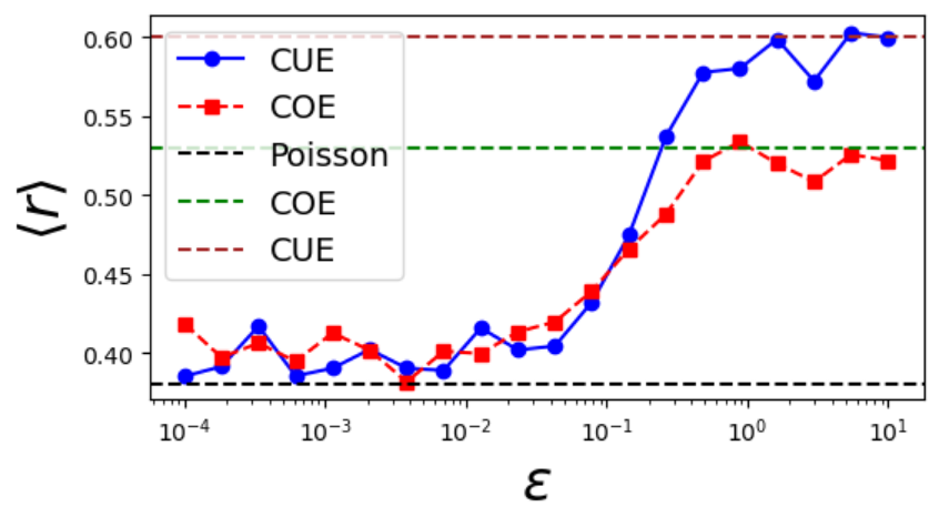
Figure 4: Level spacing ratio of RMTE model

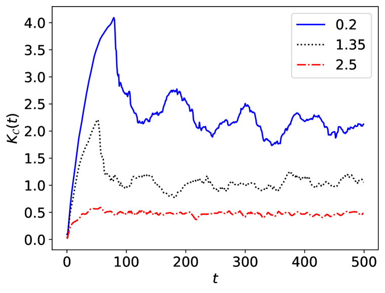
(a)

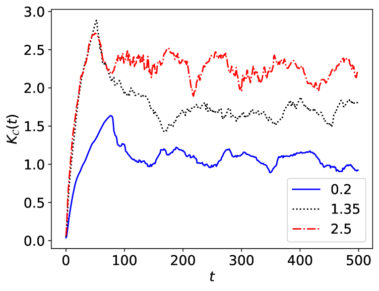
(b)

Figure 5: The saturation levels of Krylov complexity flip depending on the initial operator in the transverse Ising model. We choose a spin length $L=6,$ and $J=h_{x}=1$ in the Hamiltonian. In (a), the initial operator is $S_{z}$, whereas in (b) the initial operator is $S_{x}$.

$$\mathcal{H}_{K}^{O} =\{|\mathcal{O}_{0}),|U_{F}^{\dagger}\mathcal{O}_{0}U_{F}),|(U_{F}^{\dagger})^{2}\mathcal{O}_{0}U_{F}^{2}),....\}$$

$$=\{|\mathcal{O}_{0}),|\mathcal{O}_{1}),|\mathcal{O}_{2}),....\}\,$$ (8)

where $\mathcal{O}_{j}$ denotes the Heisenberg picture operator at time $t=jT$. $|\mathcal{O})$ denotes the operator $\mathcal{O}$ as a ket in the linear space of all operators that act in $\mathcal{H}$. Note that here $U_{F}$, as a superoperator, has the action $U_{F}|\mathcal{O})=|U_{F}^{\dagger}\mathcal{O}U_{F})$. The Krylov basis is then generated by the following recursive algorithm. Define $|K_{0})=\mathcal{O}_{0})$ and

$$|K_{1})=\frac{1}{\mathfrak{h}_{1,0}}\big{[}U_{F}|K_{0})-\mathfrak{h}_{0,0}|K_{0})\big{]}$$ (9)

$$|K_{n})=\frac{1}{\mathfrak{h}_{n,n-1}}\left[U_{F}|K_{n-1})-\sum_{j=0}^{n-1}\mathfrak{h}_{j,n-1}|K_{j})\right]$$ (10)

with $\mathfrak{h}_{j,k}=(K_{j}|U_{F}|K_{k})=\dfrac{1}{D}Tr(K_{j}^{\dagger}U_{F}^{\dagger}K_{k}U_{F})$. The normalisation $\mathfrak{h}_{n,n-1}$ are the Arnoldi coefficients. With $\mathcal{O}_{j}=(U_{F}^{\dagger})^{j}\mathcal{O}_{0}U_{F}^{j}$ being the time evolved operator at (stroboscopic) time $t=jT$, the operator complexity, defined by $\mathcal{K}_{j}^{O}=(\mathcal{O}_{j}|\hat{K}|\mathcal{O}_{j})$, is given by

$$\mathcal{K}_{j}^{O} =\sum_{n=0}^{D_{K}-1}n|(K_{n}|U_{F}^{j}|K_{0})|^{2}$$

$$=\frac{1}{D^{2}}\sum_{n=0}^{D_{K}-1}n|Tr[K_{n}^{\dagger}U_{F}^{\dagger j}K_{0}U_{F}^{j}]|^{2}.$$ (11)

This gives us a direct way to compute operator complexity given the Floquet matrix and the Krylov operator basis. Using $|\mathcal{O}_{j})=\sum_{n}\phi_{n}^{j}|K_{n})$, where $\phi_{n}^{j}=(K_{n}|\mathcal{O}_{j})$ is the $n$-th operator amplitude at time $t=jT$, we can write an equivalent form of the above equation

$$\mathcal{K}_{j}^{\mathcal{O}}=\sum_{n}n\,|\phi_{n}^{j}|^{2}.$$ (12)

III Level spacing ratio

Spectral properties of the system can distinguish between integrable and chaotic systems [27, 28]. The ratio of the consecutive eigenvalues [29] for the random matrix transition ensemble described in the main text is plotted in Fig. 4. As $\epsilon$ varies, the system transitions from a regular to chaotic regime, as indicated by the ratio distributions. The level spacing ratio is defined as:

$$r_{n}=\frac{\min(s_{n},s_{n+1})}{\max(s_{n},s_{n+1})},$$ (13)

where $s_{n}=E_{n+1}-E_{n}$ represents the spacing between consecutive eigenvalues (eigenphase in case of Floquet unitary). For integrable systems, the eigenvalues tend to follow a Poisson distribution, leading to an average spacing ratio of $\langle r\rangle\approx 0.386$. In contrast, for chaotic quantum systems that follow random matrix theory statistics. For instance, systems exhibiting time-reversal symmetry and belonging to the COE(circular orthogonal ensemble) have an average ratio of $\langle r\rangle\approx 0.530$. In contrast, those in the CUE (circular unitary ensemble) have $\langle r\rangle\approx 0.599$.

IV Krylov complexity in Transverse field Ising model

The Ising Hamiltonian includes a nearest-neighbour coupling and a transverse magnetic field in the $X-Z$ plain, given by:

$$H=\sum_{k=1}^{L}(h_{x}\sigma_{k}^{x}+h_{z}\sigma_{k}^{z})-J\sum_{k=1}^{L-1}\sigma_{k}^{z}\sigma_{k+1}^{z}.$$ (14)

Here, $L$ is the chain length, $J$ is the interaction strength and $h_{x}$ and $h_{z}$ denote the components of the magnetic field. The operators $\sigma_{k}^{\alpha}$ are local Pauli Fixing $J=h_{x}=1$, the system transitions progressively from integrability to chaos as $h_{z}$ decreases from $2.5$ to $0.2.$ The flip in the saturation of complexity depending on the initial operator is shown in Fig. 5.

References

- [1] V. Balasubramanian, P. Caputa, J. M. Magan, Q. Wu, Quantum chaos and the complexity of spread of states, Physical Review D 106 (4) (2022) 046007.
- [2] D. E. Parker, X. Cao, A. Avdoshkin, T. Scaffidi, E. Altman, A universal operator growth hypothesis, Physical Review X 9 (4) (2019) 041017.
- [3] P. Nandy, A. S. Matsoukas-Roubeas, P. Martínez-Azcona, A. Dymarsky, A. del Campo, Quantum dynamics in krylov space: Methods and applications, arXiv preprint arXiv:2405.09628 (2024).
- [4] E. Rabinovici, A. Sánchez-Garrido, R. Shir, J. Sonner, Krylov complexity from integrability to chaos, Journal of High Energy Physics 2022 (7) (2022) 1–29.
- [5] E. Rabinovici, A. Sánchez-Garrido, R. Shir, J. Sonner, Krylov localization and suppression of complexity, Journal of High Energy Physics 2022 (3) (2022) 1–42.
- [6] A. A. Nizami, A. W. Shrestha, Krylov construction and complexity for driven quantum systems, Physical Review E 108 (5) (2023) 054222.
- [7] A. A. Nizami, A. W. Shrestha, Spread complexity and quantum chaos for periodically driven spin chains, Physical Review E 110 (3) (2024) 034201.
- [8] E. Rabinovici, A. Sánchez-Garrido, R. Shir, J. Sonner, Operator complexity: a journey to the edge of krylov space, Journal of High Energy Physics 2021 (6) (2021) 1–24.
- [9] B. L. Español, D. A. Wisniacki, Assessing the saturation of krylov complexity as a measure of chaos, Physical Review E 107 (2) (2023) 024217.
- [10] G. F. Scialchi, A. J. Roncaglia, D. A. Wisniacki, Integrability-to-chaos transition through the krylov approach for state evolution, Physical Review E 109 (5) (2024) 054209.
- [11] A. Dymarsky, M. Smolkin, Krylov complexity in conformal field theory, Physical Review D 104 (8) (2021) L081702.
- [12] S. Chapman, S. Demulder, D. A. Galante, S. U. Sheorey, O. Shoval, Krylov complexity and chaos in deformed sachdev-ye-kitaev models, Physical Review B 111 (3) (2025) 035141.
- [13] D. J. Yates, A. Mitra, Strong and almost strong modes of floquet spin chains in krylov subspaces, Physical Review B 104 (19) (2021) 195121.
- [14] S. C. Srivastava, S. Tomsovic, A. Lakshminarayan, R. Ketzmerick, A. Bäcker, Universal scaling of spectral fluctuation transitions for interacting chaotic systems, Physical review letters 116 (5) (2016) 054101.
- [15] F. Haake, M. Kuś, R. Scharf, Classical and quantum chaos for a kicked top, Zeitschrift für Physik B Condensed Matter 65 (1987) 381–395.
-
[16]
F. Haake, S. Gnutzmann, M. Kuś, Time Reversal and Unitary Symmetries, Springer International Publishing, Cham, 2018, pp. 15–70.
doi:10.1007/978-3-319-97580-1_2.
URL https://doi.org/10.1007/978-3-319-97580-1_2 - [17] S. Ghose, B. C. Sanders, Entanglement dynamics in chaotic systems, Physical Review A—Atomic, Molecular, and Optical Physics 70 (6) (2004) 062315.
- [18] K. Hashimoto, K. Murata, N. Tanahashi, R. Watanabe, Krylov complexity and chaos in quantum mechanics, Journal of High Energy Physics 2023 (11) (2023) 1–41.
- [19] K. Hashimoto, K.-B. Huh, K.-Y. Kim, R. Watanabe, Exponential growth of out-of-time-order correlator without chaos: inverted harmonic oscillator, Journal of High Energy Physics 2020 (11) (2020) 1–25.
- [20] T. Xu, T. Scaffidi, X. Cao, Does scrambling equal chaos?, Physical review letters 124 (14) (2020) 140602.
- [21] R. Kidd, A. Safavi-Naini, J. Corney, Saddle-point scrambling without thermalization, Physical Review A 103 (3) (2021) 033304.
- [22] M. Lombardi, A. Matzkin, Entanglement and chaos in the kicked top, Physical Review E—Statistical, Nonlinear, and Soft Matter Physics 83 (1) (2011) 016207.
- [23] V. Madhok, Comment on “entanglement and chaos in the kicked top”, Physical Review E 92 (3) (2015) 036901.
- [24] M. Lombardi, A. Matzkin, Reply to “comment on ‘entanglement and chaos in the kicked top’”, Physical Review E 92 (3) (2015) 036902.
- [25] B. N. Parlett, The symmetric eigenvalue problem, SIAM, 1998.
- [26] V. Viswanath, G. Müller, The recursion method: application to many body dynamics, Vol. 23, Springer Science & Business Media, 1994.
- [27] O. Bohigas, M.-J. Giannoni, C. Schmit, Characterization of chaotic quantum spectra and universality of level fluctuation laws, Physical review letters 52 (1) (1984) 1.
- [28] M. C. Gutzwiller, Chaos in classical and quantum mechanics, Vol. 1, Springer Science & Business Media, 2013.
- [29] Y. Y. Atas, E. Bogomolny, O. Giraud, G. Roux, Distribution of the ratio of consecutive level spacings in random matrix ensembles, Physical review letters 110 (8) (2013) 084101.