Finite element form-valued forms (I): Construction

Abstract.

We provide a finite element discretization of $\ell$-form-valued $k$-forms on triangulation in $\mathbb{R}^{n}$ for general $k$, $\ell$ and $n$ and any polynomial degree. The construction generalizes finite element Whitney forms for the de Rham complex and their higher-order and distributional versions, the Regge finite elements and the Christiansen–Regge elasticity complex, the TDNNS element for symmetric stress tensors, the MCS element for traceless matrix fields, the Hellan–Herrmann–Johnson (HHJ) elements for biharmonic equations, and discrete divdiv and Hessian complexes in [Hu, Lin, and Zhang, 2025]. The construction discretizes the Bernstein–Gelfand–Gelfand (BGG) diagrams. Applications of the construction include discretization of strain and stress tensors in continuum mechanics and metric and curvature tensors in differential geometry in any dimension.

1. Introduction

Constructing finite element spaces (and more general discrete patterns) that encode the differential structures of continuous problems has drawn growing attention in recent decades. For solving PDEs and simulating physical systems, preserving the de Rham complex (and its cohomology) provides stability, convergence, and structure-preserving properties. This viewpoint has become central in the area of Finite Element Exterior Calculus (FEEC) [3, 5, 2]. Classic finite elements for the de Rham complex, such as Nédélec and Raviart–Thomas spaces [48, 52], can be unified through the notion of Whitney forms and their higher-order extensions [37, 38, 11, 57]. These elements have a canonical form: in the lowest order case, $k$-forms are discretized on $k$-cells. These elements and their associated numerical schemes form the standard toolkit in computational electromagnetism and other $\operatorname{curl}$–$\operatorname{div}$ problems (see, e.g., recent quantum computing hardware simulations and geophysics applications [30, 1, 47, 54]). Moreover, discrete topology and discrete differential forms play a crucial role in computer graphics [56] and topological data analysis [46].

A wide range of problems involve tensors with more general symmetries (differential forms being tensors with full skew-symmetry) and more elaborate differential structures than the $\operatorname{grad}$–$\operatorname{curl}$–$\operatorname{div}$ operators in the de Rham setting. For instance, elasticity typically introduces symmetric $(0,2)$-tensors as strain and stress, while in differential geometry, the metric is a symmetric $(0,2)$-tensor and the Riemannian curvature, interpreted as a $(0,4)$-tensor, obeys multiple symmetries (skew-symmetry in the first two and the last two indices, symmetry between those two groups, plus the algebraic Bianchi identity). Related constructions (Ricci, Einstein, Weyl tensors, etc.) arise in general relativity, continuum defects, network theories, and beyond. Inspired by the canonical form and wide applications of discrete or finite element differential forms on triangulation, a natural question is

Are there discrete analogues of such tensors with symmetries and differential structures?

(1)

For these tensorial objects, the Bernstein–Gelfand–Gelfand (BGG) sequences play a role analogous to that of the de Rham complex for differential forms. Originally studied in algebraic geometry and representation theory [8, 15, 29], BGG sequences have recently been brought into analytic contexts and numerical analysis [4, 7, 14, 5]. Corresponding finite element discretizations have been explored in various works [16, 18, 20, 19, 17, 41, 39, 32, 10, 25, 24, 40], mostly focusing on conforming elements (piecewise polynomials with certain high intercell continuity). Except for one approach on cubical meshes using tensor product structures [10], these constructions are either dimension-specific or restricted to particular slots in a complex. No systematic approach exists to cover all form indices in arbitrary dimension. More importantly, while Whitney forms for the de Rham complex exhibit a clear topological structure, such structures have yet to be fully discovered for tensors, either generally or more specifically in BGG-type constructions [7].

The work in this paper aims to answer a more specific version of (1):

Are there canonical finite elements for form-valued forms and BGG complexes on triangulation?

(2)

In other words, we aim to design finite elements that reflect the same differential and cohomological properties as their continuous counterparts, while also demonstrating discrete topological/geometry structures comparable to Whitney forms in the de Rham context. Requiring these properties is not only mathematically appealing but also crucial for robust numerical solutions for tensor-valued problems, problems involving intrinsic geometry (e.g., shells, continuum defects, numerical relativity), and for discrete structures (e.g., networks, graphs, [46]).

Similar to that finite element differential forms were built based on works by Nédéléc [48], Raviart-Thomas [52], Brezzi-Douglas-Marini [13], etc., many building blocks are also available for formed-valued forms. Christiansen’s reinterpretation of Regge calculus as a finite element [23] elegantly fits into a discrete elasticity complex. The piecewise-constant metric yields a conic (distributional) curvature, matching the angle-deficit interpretation of Regge geometry. One may see the Christiansen-Regge complex as the canonical discretization for that complex, for the canonical forms of the degrees of freedom, for the discrete geometric interpretation, and for the formal self-adjointness. The cohomology and extensions of the Christiansen-Regge complex can be found in [26].

Independently, Schöberl and collaborators developed distributional finite elements for equilibrated error estimators [12] and for continuum mechanics, giving rise to the TDNNS method for elasticity [51] and the MCS method [33] for fluids. The classical work of the Hellan–Herrmann–Johnson (HHJ) element [35, 36, 43] for biharmonic plate problems can be also interpreted in this spirit [49]. These methods incorporate distributional derivatives and certain vector or matrix versions of Dirac measures. A systematic discussion on distributional de Rham complexes can be found in [45].

New finite element and distributional spaces were needed to derive the Hessian and divdiv complexes in three dimensions [42]. The Hessian complex starts with a Lagrange element, followed by Dirac measures. The divdiv complex are formal adjoint of the Hessian complex. The shape function spaces have a Koszul-type construction. Moreover, [42] used a diagram chase approach to establish the cohomology of the discrete complexes.

On the continuous level, 0-form-valued and $n$-formed valued de Rham complexes (the former is just the de Rham complex and the latter can be identified with a de Rham complex if a volume element is fixed) fit in the same diagram as BGG complexes (see Figure 1). On the discrete level, the Whitney forms for the de Rham complex [11, 37, 5], the dual Whitney forms [12], the Christiansen-Regge element [23], and the discrete Hessian and divdiv complexes [42] completes a diagram in three dimensions with a canonical pattern (see Figure 2).

$\begin{array}[]{c}\operatorname{Alt}^{-1,-1}\\ \\ \\ \end{array}\begin{array}[]{c}\leavevmode\hbox to35.12pt{\vbox to6.67pt{\text{[drawing]}}}\vskip-8.5359pt\\ \vskip-5.69046pt\leavevmode\hbox to35.12pt{\vbox to23.74pt{\text{[drawing]}}}\vskip-5.69046pt\\ \leavevmode\hbox to35.12pt{\vbox to6.67pt{\text{[drawing]}}}\end{array}\begin{array}[]{c}\\ \\ \operatorname{Alt}^{0,0}~~\longrightarrow~~\operatorname{Alt}^{1,0}~~\longrightarrow~~\operatorname{Alt}^{2,0}~~\longrightarrow~~\operatorname{Alt}^{3,0}\end{array}$

$\begin{array}[]{c}\operatorname{Alt}^{0,0}\\ \\ \\ \end{array}$ $\begin{array}[]{c}\longrightarrow\\ \swarrow\\ \longrightarrow\end{array}$ $\begin{array}[]{c}\\ \\ \operatorname{Alt}^{1,1}\end{array}$ $\begin{array}[]{c}\\ \\ \longrightarrow\end{array}$ $\begin{array}[]{c}\\ \\ \operatorname{Alt}^{2,1}\end{array}$ $\begin{array}[]{c}\\ \\ \longrightarrow\end{array}$ $\begin{array}[]{c}\\ \\ \operatorname{Alt}^{3,1}\end{array}$
$\begin{array}[]{c}\operatorname{Alt}^{0,1}\\ \\ \\ \end{array}$ $\begin{array}[]{c}\longrightarrow\\ \\ \\ \end{array}$ $\begin{array}[]{c}\operatorname{Alt}^{1,1}\\ \\ \\ \end{array}$ $\begin{array}[]{c}\longrightarrow\\ \swarrow\\ \longrightarrow\end{array}$ $\begin{array}[]{c}\\ \\ \operatorname{Alt}^{2,2}\end{array}$ $\begin{array}[]{c}\\ \\ \longrightarrow\end{array}$ $\begin{array}[]{c}\\ \\ \operatorname{Alt}^{3,2}\end{array}$
$\begin{array}[]{c}\operatorname{Alt}^{0,2}\\ \\ \\ \end{array}$ $\begin{array}[]{c}\longrightarrow\\ \\ \\ \end{array}$ $\begin{array}[]{c}\operatorname{Alt}^{1,2}\\ \\ \\ \end{array}$ $\begin{array}[]{c}\longrightarrow\\ \\ \\ \end{array}$ $\begin{array}[]{c}\operatorname{Alt}^{2,2}\\ \\ \\ \end{array}$ $\begin{array}[]{c}\longrightarrow\\ \swarrow\\ \longrightarrow\end{array}$ $\begin{array}[]{c}\\ \\ \operatorname{Alt}^{3,3}\end{array}$
$\begin{array}[]{c}\operatorname{Alt}^{0,3}~~\longrightarrow~~\operatorname{Alt}^{1,3}~~\longrightarrow~~\operatorname{Alt}^{2,3}~~\longrightarrow~~\operatorname{Alt}^{3,3}\\ \\ \\ \end{array}\begin{array}[]{c}\leavevmode\hbox to35.12pt{\vbox to6.67pt{\text{[drawing]}}}\vskip-8.5359pt\\ \vskip-5.69046pt\leavevmode\hbox to35.12pt{\vbox to23.74pt{\text{[drawing]}}}\vskip-5.69046pt\\ \leavevmode\hbox to35.12pt{\vbox to6.67pt{\text{[drawing]}}}\end{array}\begin{array}[]{c}\\ \\ \operatorname{Alt}^{4,4}\end{array}$

Figure 1. De Rham and BGG complexes with form-valued forms in $\mathbb{R}^{3}$ on the continuous level in a unified language. Here $\operatorname{Alt}^{k,\ell}$ stands for $\ell$-form-valued $k$-forms with certain symmetries. The complexes are the 3-form-valued de Rham complex, the Hessian complex, the elasticity complex, the divdiv complex, and the de Rham complex, respectively. The spaces $\operatorname{Alt}^{-1,-1}$ and $\operatorname{Alt}^{4,4}$ are trivial in 3D.

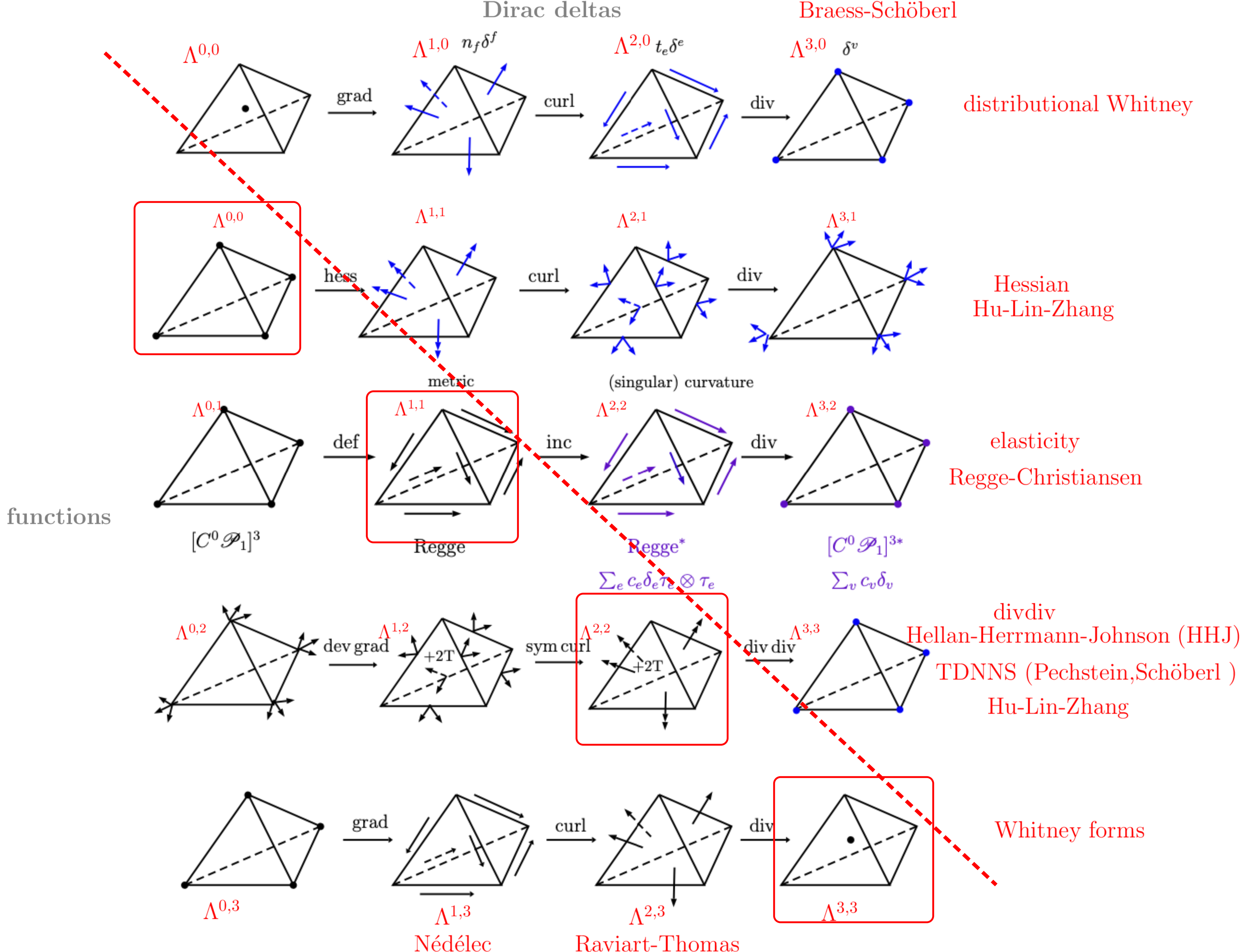
Figure 2. Finite elements (including currents) of the lowest order for Figure 2. The first row is the distributional de Rham complex (dual Whitney forms) [12, 45]; the last row consists of Whitney forms; the elasticity complex is discretized by the Christiansen–Regge complex [23]; the Hessian and divdiv complexes are due to [42].

In this paper, we identify the patterns in Figure 2 and extends them to any dimension, any form-valued form, and any polynomial degree. Moreover, we discretize the iterated BGG constructions (leading to the $\operatorname{grad}\operatorname{curl}$ complex, the $\operatorname{curl}\operatorname{div}$ complex, and the $\operatorname{grad}\operatorname{div}$ complex in 3D; see Figure 3). The complexes (Figure 4) glue together Whitney forms and the MCS element with high-order differentials.

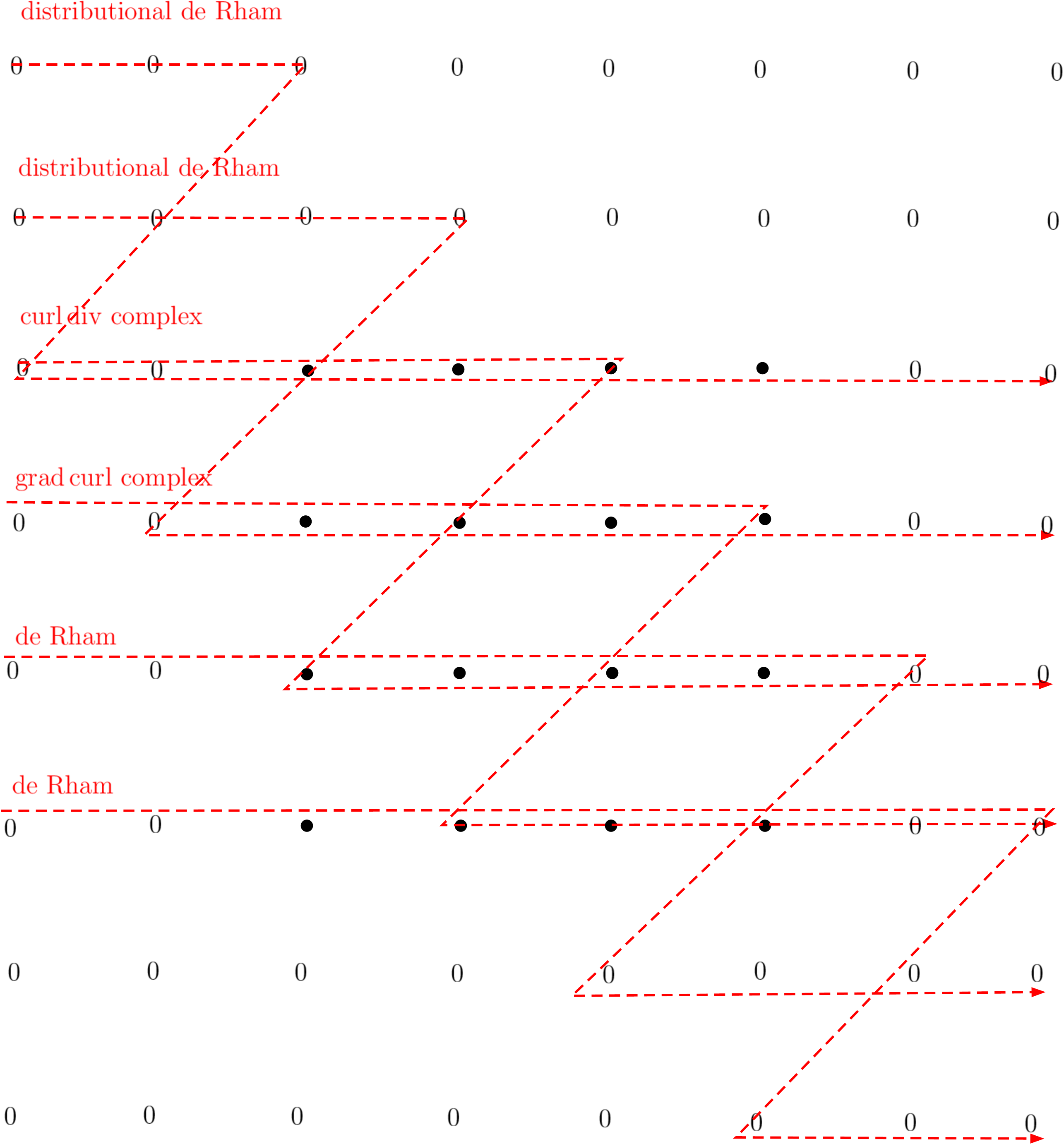
Figure 3. Iterated BGG constructions. The dots denote spaces $C^{\infty}\otimes\operatorname{Alt}^{k,\ell}$ with $0\leq k,\ell\leq 3$. The diagram is extended by zero.

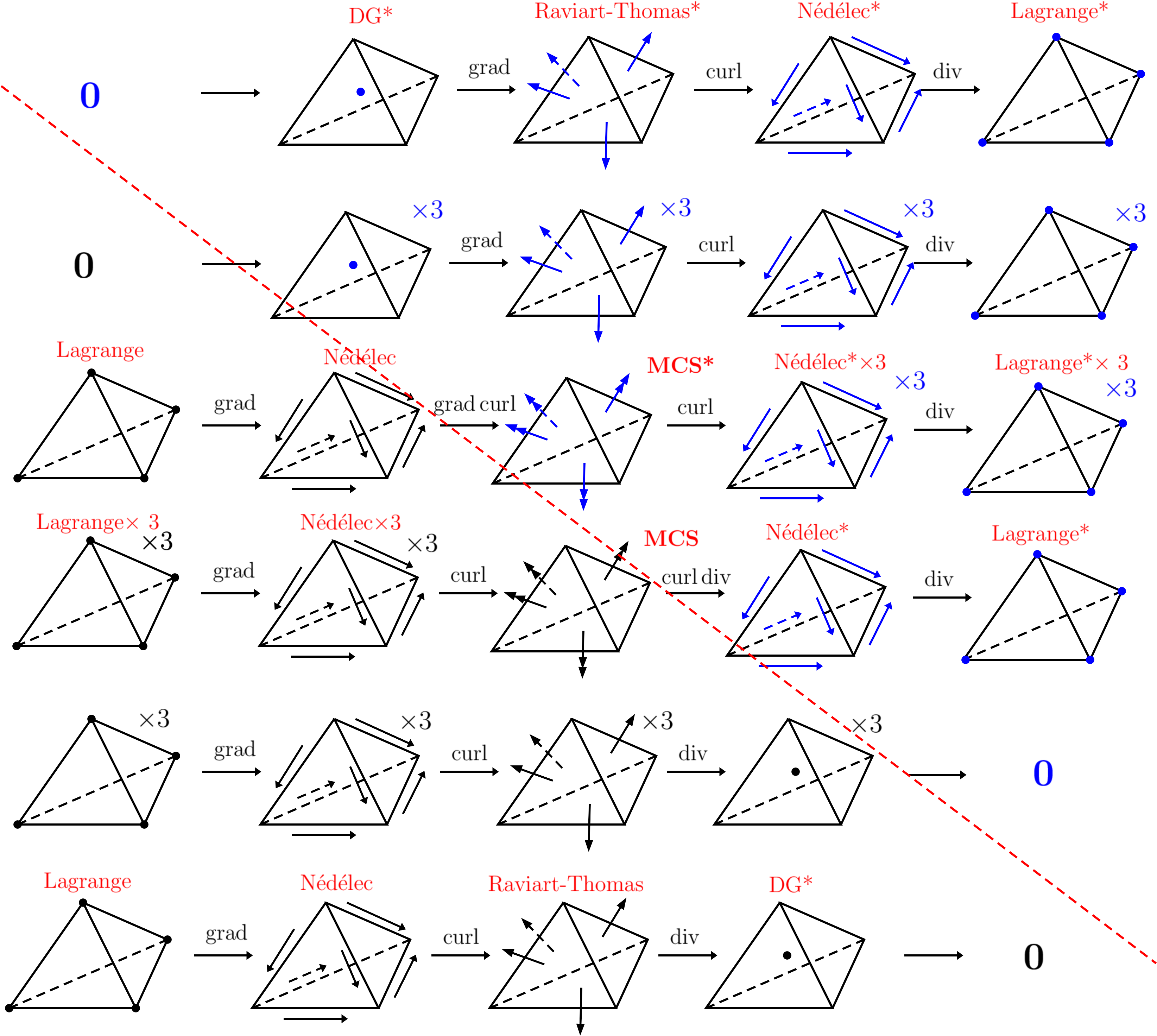
Figure 4. Distributional finite element complexes for the iterated BGG constructions.

We show the unisolvency of the resulting finite element spaces. This paper leaves the complex and cohomological issues open, i.e., in this paper, we do not prove that the resulting spaces fit in a complex and their cohomology is isomorphic to the continuous versions (although they do in three and lower dimensions). This is because some of the differential operators have to be interpreted discretely, and a full explanation is beyond the scope of this paper. However, we provide a dimension count as a strong indication that such results will hold in any dimensions.

Before diving into details of the construction, we mention motivations for investigating a general construction in arbitrary dimensions.

• Identifying the canonical patterns in general dimensions for general forms contributes to understanding constructions and applications in three dimensions.

• Important problems from differential geometry and relativity require discretizing tensor fields (such as the metric and various notions of curvature tensors) in four and higher dimensions.

• The twisted complexes [7, 14], which involve all the spaces in the BGG diagram, play a fundamental role in their own right. The twisted complexes incorporate richer physics and geometry. For example, the twisted complex models micropolar and Cosserat models while the BGG complex is for standard elasticity [14]; the twisted complex involves Riemann-Cartan geometry with curvature and torsion, while the torsion is eliminated in the BGG complex [26]. Applications require discretizing the twisted complexes [28]. The general construction in this paper discretizes the entire diagram, and therefore sheds light on discretizing generalized models in micropolar continuum, Riemann-Cartan geometry and continuum defects [58, 60, 59] etc.

• Cliques (analogues of simplices) of any dimensions exist on graphs or hypergraphs [9]. A simplicial construction with full generality sheds light on investigating objects and applications from graph and network theory, such as the notion of graph curvature.

Concerning the last point, Hodge-Laplacian and discrete differential forms can be established on graphs [46]. The theory has a close relation with the lowest order Whitney forms as they share the same degrees of freedom. To carry tensor finite elements to other discrete structures such as graphs, one desires intrinsic finite elements with canonical degrees of freedom and geometric and topological interpretations. This is another reason for the preference of a construction mimicking the Whitney forms with relaxed conformity (for the de Rham complex, the Whitney forms happen to have enough conformity for $L^{2}$ spaces with exterior derivatives in $L^{2}$; however, this is not the case for the BGG complexes).

1.1. Overview of the construction

Each BGG complex involves a “zig-zag” at some slot, connecting two rows of the diagram. From the examples in Figure 2 (see also Figure 1), we see that each BGG complex consists of finite element spaces (piecewise polynomials) before the zig-zag, and then Dirac measures of certain types (referred to as currents hereafter) after it. The sequence of Whitney forms and its dual are two special cases, where all spaces are finite elements or all spaces are currents, respectively. To generalize this pattern in the general construction, each sequence is also split into two parts: first the finite elements and then the currents. The construction of currents is relatively straightforward, as we can extend the sequences via derivatives. However, constructing the finite element spaces calls for special care in choosing local shape functions and degrees of freedom that match each other (unisolvency) and yield the desired interelement continuity.

Generalized trace operators. For a finite element space, specifying the conformity (and hence the degrees of freedom) is essential. For the Whitney forms, the conformity condition demands that the trace (see (3.1)) of a differential form from both sides of a face is single-valued on that face. Correspondingly, the degrees of freedom for Whitney forms can be given by moments of this trace over subcells. The first challenge for form-valued forms is to generalize the notion of the trace. A straightforward approach is to project each vector onto the face’s tangent space (see $\iota^{\ast}\iota^{\ast}$ below). However, this is not necessarily what we need. For example, consider the first space in the elasticity complex, which is in $\mathrm{Alt}^{0,1}$ (1-form-valued 0-forms). The $\iota^{\ast}\iota^{\ast}$-trace vanishes at vertices. Yet the canonical Christiansen–Regge complex starts with a Lagrange space, requiring vertex evaluations.

To resolve this, we introduce generalized trace operators. In particular, we allow evaluating a $k$-form on an $m$-dimensional cell where $m<k$ (via the operator $\jmath^{*}$ (3.5)). The idea is to use tangent vectors as much as possible. For example, to evaluate a 3-form on a 1-dimensional cell, we feed its single tangent vector plus two vectors normal to the cell into the 3-form. This definition sits between the classical trace (which feeds only tangent vectors) and the restriction operator (which can feed any vectors).

For iterated BGG complexes, we must generalize further, leading to $\jmath^{*}_{[p]}$ (the above case corresponds to $p=1$). Increasing $p$ moves the definition closer to the restriction operator, allowing one ($p=2$) or more ($p\geq 3$) tangent vectors to remain unused. In the example of evaluating a 3-form on a 1D cell, $\jmath^{*}_{[2]}$ permits either tangent or normal vectors. On a 1D cell, this reduces effectively to the restriction operator. On 2D cells, for $p=2$, one must feed at least one tangent vector to the 3-form, while the remaining two slots can be tangent or normal; for $p=3$, $\jmath^{*}_{[p]}$ boils down to the restriction. The notation has not appeared in existing literature on finite elements in three dimensions, as the first non-trivial examples appear in four dimensions. The definition of the generalized traces and their properties are discussed in Section 3.

These generalized traces recover existing elements such as TDNNS, MCS, Regge, Hu–Lin–Zhang in 3D, and enable new constructions in higher dimensions.

The overall idea behind constructing finite elements in this paper is to modify the Whitney forms, following the following steps.

Step 1: $\iota^{\ast}\iota^{\ast}$-conforming elements. For $\ell$-form-valued $k$-forms, we begin by tensoring Whitney $k$-forms with alternating $\ell$-forms, giving $\mathcal{P}^{-}\mathrm{Alt}^{k,\ell}:=\mathcal{P}^{-}\mathrm{Alt}^{k}\otimes\mathrm{Alt}^{\ell}$. The resulting space is $\iota^{\ast}\rho^{\ast}$-conforming (where $\rho^{\ast}$ is the restriction operator). We then weaken continuity to obtain an $\iota^{\ast}\iota^{\ast}$-conforming space. For instance, to build 1-form-valued 1-forms in 3D, we start with three copies of the Nédélec space (tangential continuity) and weaken the continuity, leading to tangential–tangential continuity. This general procedure is possible because one can move certain degrees of freedom from lower-dimensional subcells to higher-dimensional ones. The resulting finite element spaces $C_{\iota^{*}\iota^{*}}\mathcal{P}^{-}\mathrm{Alt}^{k,\ell}$ are spelled out in Proposition 4.1.

Step 2: Symmetry reduction. The spaces from Step 1 do not yet reflect the tensor symmetries in the BGG complexes. We therefore reduce these spaces to lie in $\mathcal{N}(\mathcal{S}_{\dagger})$, which appears in the BGG diagrams. This requires reducing both the shape function spaces and their degrees of freedom.

To reduce the local shape function spaces, we verify that the BGG machinery is compatible with the polynomial spaces $\mathcal{P}^{-}\mathrm{Alt}^{k,\ell}$; i.e., $\mathcal{S}_{\dagger}$ maps onto from $\mathcal{P}^{-}\mathrm{Alt}^{k,\ell}$ to $\mathcal{P}^{-}\mathrm{Alt}^{k-1,\ell+1}$ (Lemma 2.2).

The degrees of freedom for $\mathcal{P}^{-}\mathrm{Alt}^{k,\ell}$ involve moments against bubbles on each subcell. We remove certain bubbles likewise. Consequently, the degrees of freedom for the reduced finite elements can be defined by moments against the reduced bubble spaces. The key is to check that $\mathcal{S}_{\dagger}$ indeed maps onto from $\mathcal{B}^{-}\mathrm{Alt}^{k,\ell}$ to $\mathcal{B}^{-}\mathrm{Alt}^{k-1,\ell+1}$ (see (4.2) and Lemma 4.3).

This process yields spaces $C_{\iota^{\ast}\iota^{\ast}}\mathcal{P}^{-}\mathbb{W}^{k,\ell}$ together with their degrees of freedom, described in Proposition 4.2.

Step 3: $\iota^{\ast}\jmath^{\ast}$-conforming elements. We then move certain degrees of freedom from higher-dimensional subcells to lower-dimensional ones, improving the continuity of the finite element space. This works because:

1. The total dimension of the space remains unchanged.

2. Single-valuedness on lower-dimensional subcells guarantees single-valuedness on higher-dimensional subcells.

This procedure applies to the full $\mathrm{Alt}^{k,\ell}$ spaces (Proposition 4.4) and to the reduced ${\mathbb{W}}^{k,\ell}$ spaces (Proposition 4.5).

We apply the same recipe to obtain spaces $\mathcal{P}^{-}{\mathbb{W}}_{[p]}^{k,\ell}$ in the iterated BGG complexes (Proposition 4.6).

The above recipe is demonstrated in Figures 5, 6, 7 and 8 for the Regge, HLZ, MCS, and HHJ (TDNNS) elements, respectively.

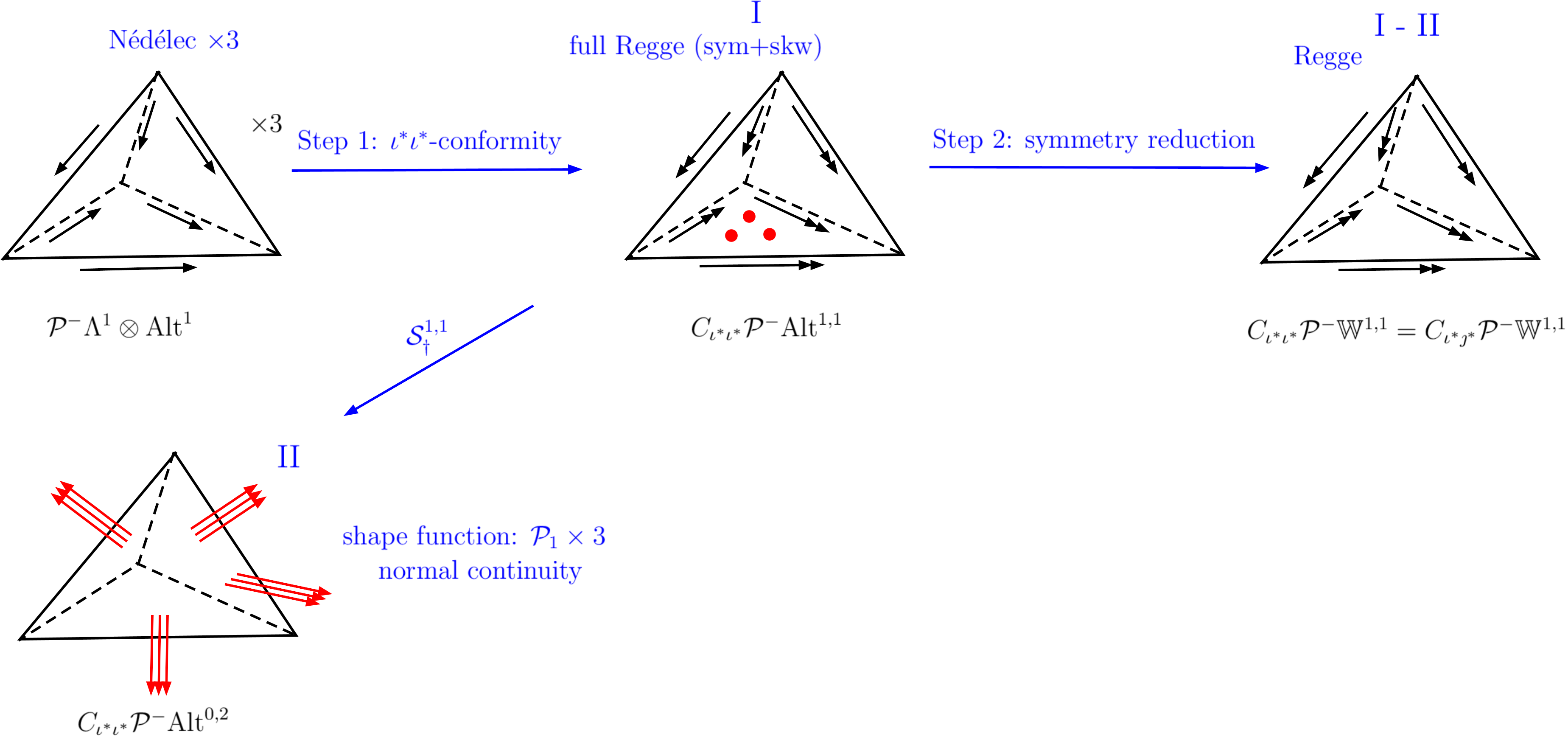
Figure 5. Deriving the Regge element (tangential-tangential continuity) from a vector-valued Nédélec element (tangential continuity). Step 1: weakening the continuity of the Nédélec element to tangential-tangential. Step 2: eliminating the face degrees of freedom by those of a weakened vector Lagrange element connected by a $\mathcal{S}_{\dagger}$ operator.

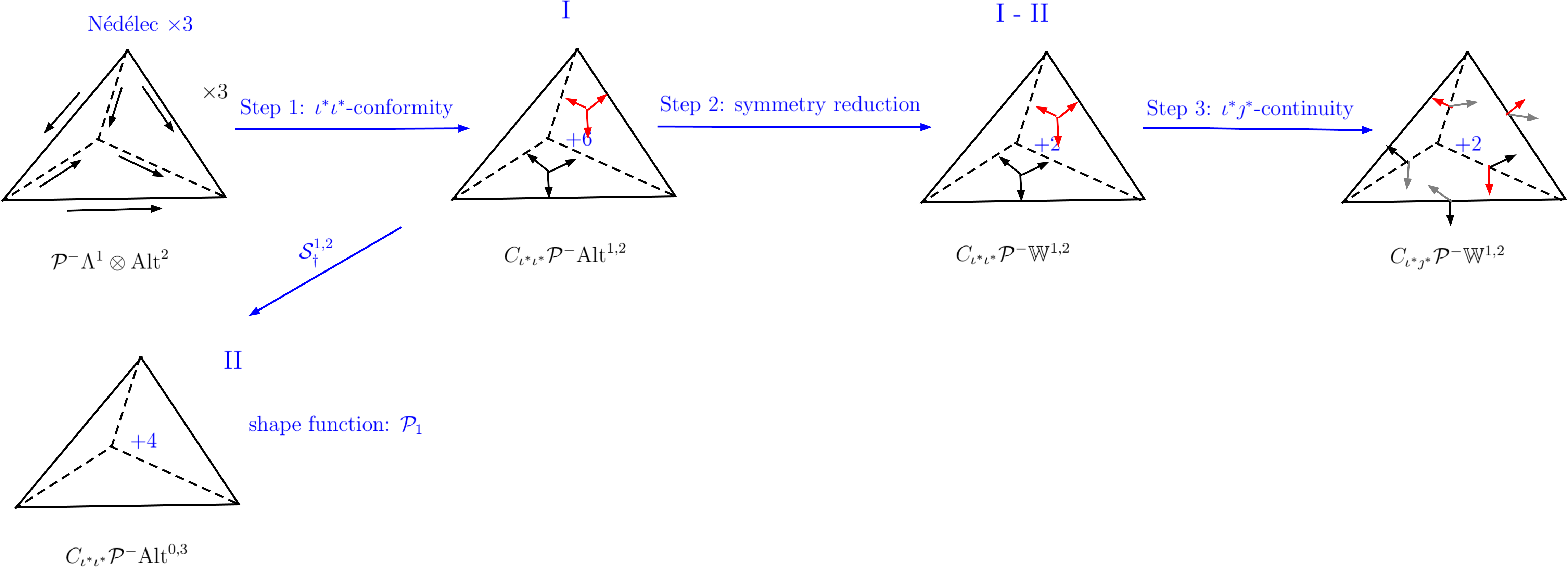
Figure 6. Deriving the Hu-Lin-Zhang element (tangential-normal continuity) from a vector-valued Nédélec element (tangential continuity). Step 1: weakening the continuity of the Nédélec element to tangential-normal. Step 2: eliminating part of the interior degrees of freedom by those of a $\mathcal{P}_{1}$ connected by an $\mathcal{S}_{\dagger}$ operator. Step 3: moving the three degrees of freedom on each face to the three edges of the face; each edge gathers two tangential-normal degrees of freedom from its two neighbouring faces.
In general, we obtain $C_{\iota^{*}\jmath^{*}}\mathcal{P}^{-}\mathrm{Alt}^{k,\ell}(K)$ from $C_{\iota^{*}\iota^{*}}\mathcal{P}^{-}\mathrm{Alt}^{k,\ell}(K)$ by moving degrees from $\ell$-dimensional cells to $k$-dimensional ones. On each $\ell$-face $F$, the degrees of freedom are the inner product with respect to the space $\mathcal{P}^{-}\mathrm{Alt}^{k}(F)$. To see that these degrees of freedom can be relocated to $k$-cells, note that each $\sigma\in\mathcal{T}_{k}(F)$ receives $\binom{n-k}{\ell-k}$ degrees of freedom (one from each $\ell$-face containing $\sigma$), which is exactly the dimension of $\mathrm{Alt}^{\ell-k}(\sigma^{\perp})$.

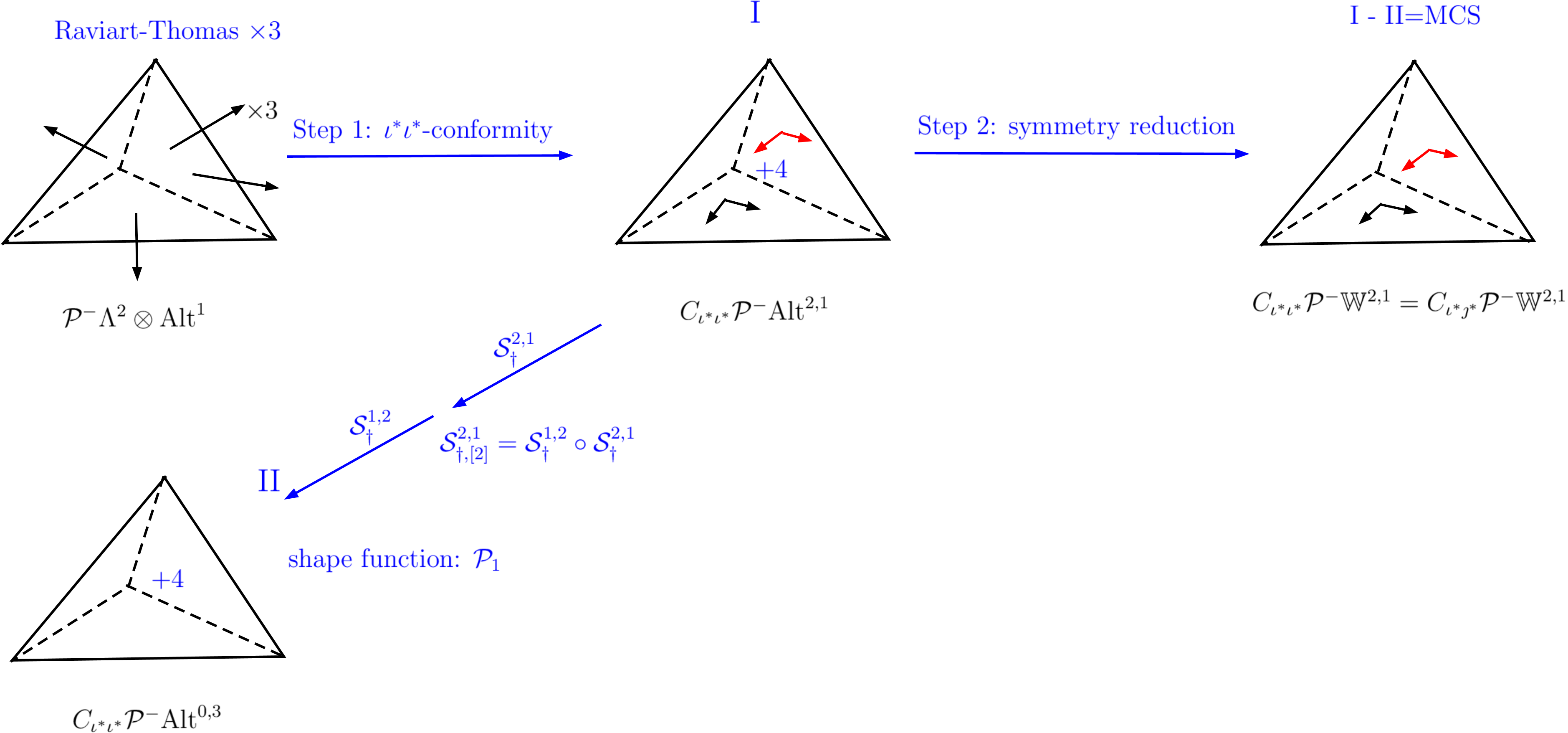
Figure 7. Deriving the MCS element (normal-tangential continuity) from a vector-valued Raviart–Thomas element (normal continuity). Step 1: weakening the continuity of the Raviart–Thomas element to normal-tangential. Step 2: eliminating part of the interior degrees of freedom by those of a $\mathcal{P}_{1}$ connected by an $\mathcal{S}_{\dagger,[2]}$ operator. Note that the MCS element appears in an iterated BGG construction as $k=2,\ell=1$ and $k>\ell$. Thus the reduction is by a space down two rows.

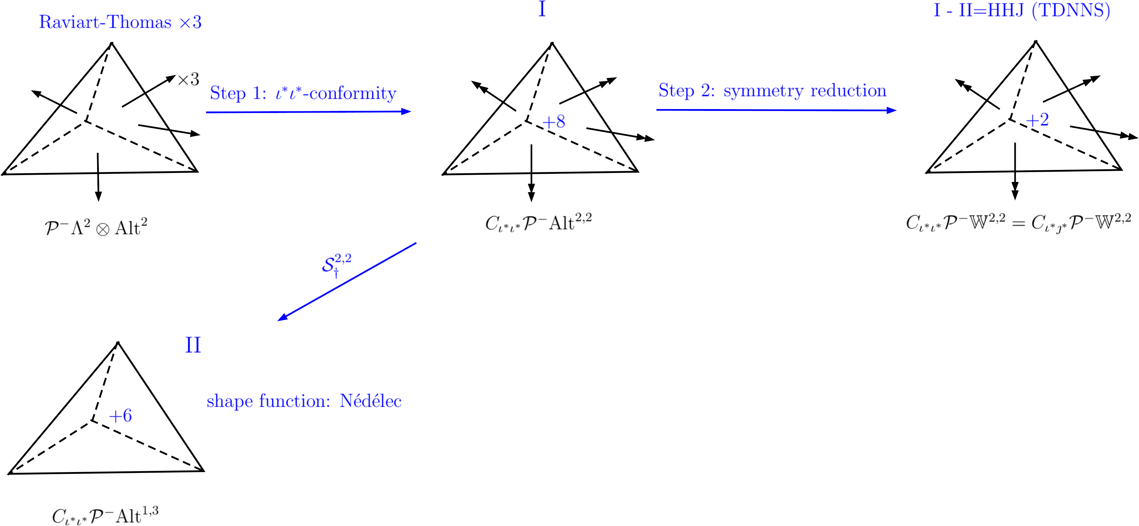
Figure 8. Deriving the HHJ (TDNNS) element (normal-normal continuity) from a vector-valued Raviart–Thomas element (normal continuity). Step 1: weakening the continuity of the Raviart–Thomas element to normal-normal. Step 2: eliminating part of the interior degrees of freedom by Nédélec shape functions connected by a $\mathcal{S}_{\dagger}$ operator.

Finally, higher-order constructions (including the family $\mathcal{P}\mathrm{Alt}_{[p]}^{k,\ell}$ and $\mathcal{P}{\mathbb{W}}_{[p]}^{k,\ell}$) follow analogously, using the same sequence of steps.

Remarks on complexes and cohomologies. For a complex

where $V^{i},\forall i$ is a finite dimensional vector space, a necessary condition for it to be exact is that the Euler characteristic is zero. That is,

(1.1) $$\sum_{i=0}^{n}(-1)^{i}\dim V^{i}=0.$$

Although in this paper, we do not prove that the cohomologies of the finite element complexes are isomorphic to the continuous versions (except for dimension less than or equal to three, which was proved in [42]), we show that (1.1) holds for all the complexes when the domain has trivial topology. This should be a strong indication that the complexes indeed have correct cohomology. A detailed investigation on the operators and cohomology is left for future work.

1.2. Notations

Let $V$ be a vector space. We use $\operatorname{Alt}^{k}(V)$ to denote the algebraic alternating $k$-forms on $V$, and $\operatorname{Alt}^{k,\ell}(V):=\operatorname{Alt}^{k}(V)\otimes\operatorname{Alt}^{\ell}(V)$. When there is no danger of confusion, we also drop $V$ and write $\operatorname{Alt}^{k}$ and $\operatorname{Alt}^{k,\ell}$. Then the space $C^{\infty}(\Omega)\otimes\operatorname{Alt}^{k}$ consists of smooth differential $k$-forms on a manifold $\Omega$. We use $d^{{\scriptscriptstyle\bullet}}$ to denote the exterior derivative $d^{k}:C^{\infty}\otimes\Lambda^{k,\ell}\to C^{\infty}\otimes\Lambda^{k+1,\ell}$. Note that $d^{{\scriptscriptstyle\bullet}}$ acts on the first index ($k$, rather than $\ell$).

Hereafter, $\mathcal{T}$ is a triangulation and $\mathcal{T}_{<n}$ denotes the set of all subsimplices of $\mathcal{T}$ with dimension less than $n$. Similarly, we define $\mathcal{T}_{>n},\mathcal{T}_{\leq n},\mathcal{T}_{\geq n}$, and define $\mathcal{T}_{[a:b]}:=\mathcal{T}_{\geq a}\cap\mathcal{T}_{\leq b}$.

We introduce notation for several linear algebraic operations on $\mathbb{R}^{n\times n}$:

• $\operatorname{skw}:\mathbb{M}\to\mathbb{K}$ and $\operatorname{sym}:\mathbb{M}\to\mathbb{S}$ denote taking the skew-symmetric and symmetric part of a matrix.

• $\operatorname{tr}:\mathbb{M}\to\mathbb{R}$ is the trace, given by summing the diagonal entries of a matrix.

• $I:\mathbb{R}\to\mathbb{M}$ is defined by $I(u):=uI$, identifying a scalar $u$ with the corresponding diagonal matrix.

• $\operatorname{dev}:\mathbb{M}\to\mathbb{T}$ is the deviator (trace-free part), $\operatorname{dev}(u):=u-\tfrac{1}{n}\operatorname{tr}(u)I$.

In three dimensions only, there is an isomorphism between skew-symmetric matrices in $\mathbb{K}$ and vectors in $\mathbb{V}$ via

$$\operatorname{mskw}\left(\begin{array}[]{c}v_{1}\\ v_{2}\\ v_{3}\end{array}\right)=\begin{pmatrix}0&-v_{3}&v_{2}\\ v_{3}&0&-v_{1}\\ -v_{2}&v_{1}&0\end{pmatrix}.$$

This map $\operatorname{mskw}:\mathbb{V}\to\mathbb{K}$ is an isomorphism satisfying $\operatorname{mskw}(v)\,w=v\times w$ for any $v,w\in\mathbb{V}$; the vector $v$ is called the axial vector of $\operatorname{mskw}(v)$. We also define $\operatorname{vskw}:=\operatorname{mskw}^{-1}\circ\operatorname{skw}:\mathbb{M}\to\mathbb{V}$, taking a matrix to the axial vector of its skew-symmetric part.

Finally, let $S:\mathbb{M}\to\mathbb{M}$ be the linear map given by $S(u):=u^{T}-\operatorname{tr}(u)\,I$. One can verify that $S$ is invertible for any $n>1$.

We summarize the notations and terms that will be used below, see Tables 2, 3 and 1, with references to the place where they first appear.

Table 1. General notations.

$\Omega$	$n$ dimensional domain
$\mathcal{T}$	triangulation of $\Omega$
$\mathcal{T}_{s},\mathcal{T}_{\leq a},\mathcal{T}_{<a},\mathcal{T}_{>a},\mathcal{T}_{\geq a},\mathcal{T}_{[a,b]}$	the collection of the faces
	with dimension $s,\leq a,<,\geq a,>a$ and $\in[a,b]$
$\mathcal{H}_{dR}$	de Rham cohomology
$\lambda_{i}$	barycentric coordinates
$\phi_{\sigma}$, (4.3), p.4.3	Whitney form
$[n]$	$\{1,2,\cdots,n\}$
$X(n,k)$	increasing $k$ sets in $\{1,2,\cdots,n\}$
DoFs	abbreviation for degrees of freedom
BGG	Bernstein-Gelfand-Gelfand

Table 2. Notations for continuous and discrete spaces.

Forms
$\operatorname{Alt}^{k}$	alternating $k$-forms
$\mathcal{P}_{r}\mathrm{Alt}^{k}$, Section 6, p.6	polynomial $k$-forms
$\mathcal{B}_{r}\mathrm{Alt}^{k}$, Section 6, p.6	bubble space of polynomial $k$-forms
$\mathcal{P}_{r}^{-}\mathrm{Alt}^{k}$, Section 6, p.6	incomplete polynomial $k$-forms
$\mathcal{B}_{r}\mathrm{Alt}^{k}$, Section 6, p.6	bubble space of incomplete polynomial $k$-forms
$N^{\ell}(\sigma,K)$, (4.5), p.4.5	auxiliary space for bubbles
Form-valued Forms
$\operatorname{Alt}^{k,\ell}:=\operatorname{Alt}^{k}\otimes\operatorname{Alt}^{\ell}$	alternating $\ell$-form-valued alternating $k$-forms (($k,\ell$) forms)
${\mathbb{W}}^{k,\ell}$, (2.6), p.2.6	subspace of $\operatorname{Alt}^{k,\ell}$ in either $\mathcal{N}(\mathcal{S}^{{\scriptscriptstyle\bullet}})$ or $\mathcal{N}(\mathcal{S}^{{\scriptscriptstyle\bullet}}_{\dagger})$
${\mathbb{W}}^{k,\ell}_{[p]}$, (2.20), p.2.20	subspace of $\operatorname{Alt}^{k,\ell}$ in $\mathcal{N}(\mathcal{S}^{{\scriptscriptstyle\bullet}}_{\dagger,[p]})$,
$\widetilde{{\mathbb{W}}}^{k,\ell}_{[p]}$, (2.21), p.2.21	subspace of $\operatorname{Alt}^{k,\ell}$ in $\mathcal{N}(\mathcal{S}^{{\scriptscriptstyle\bullet}}_{[p]})$
$\mathcal{P}^{-}\mathrm{Alt}^{k,\ell}$, (4.1), p.4.1	Whitney $(k,\ell)$ forms
$\mathcal{B}^{-}\mathrm{Alt}^{k,\ell}$, (4.2), p.4.2	Bubbles of Whitney $(k,\ell)$ forms
$\mathcal{P}_{r}^{-}\operatorname{Alt}^{k,\ell}$, (2.14), p.2.14	incomplete polynomial $(k,\ell)$ forms
$\mathcal{B}_{r}^{-}\mathrm{Alt}^{k,\ell}$, (6.6), p. 6.6	bubbles of incomplete polynomial $(k,\ell)$ forms
$\mathcal{P}_{r}^{-}{\mathbb{W}}^{k,\ell}$, (2.15), p.2.15	incomplete polynomial subspace in $\mathcal{N}(\mathcal{S}^{{\scriptscriptstyle\bullet}}_{\dagger})$
$\mathcal{P}_{r}^{-}{\mathbb{W}}^{k,\ell}_{[p]}$, Lemma 2.5, p.2.5	incomplete polynomial subspace in $\mathcal{N}(\mathcal{S}^{{\scriptscriptstyle\bullet}}_{\dagger,[p]})$
$\mathcal{P}_{r}\mathrm{Alt}^{k,\ell}$	polynomial $(k,\ell)$ forms $\mathcal{P}_{r}\otimes\mathrm{Alt}^{k,\ell}$
$\mathcal{B}_{r}\mathrm{Alt}^{k,\ell}$, (6.11), p.6.11	bubbles of polynomial $(k,\ell)$ forms
$\mathcal{P}_{r}{\mathbb{W}}^{k,\ell}$, $\mathcal{P}_{r}{\mathbb{W}}^{k,\ell}_{[p]}$	polynomial subspaces $\mathcal{P}_{r}\otimes{\mathbb{W}}^{k,\ell}$ and $\mathcal{P}_{r}\otimes{\mathbb{W}}^{k,\ell}_{[p]}$

Table 3. Notations for the operators.

$d$	differential operators for forms and form-valued forms
$\mathcal{S}$, (2.1), p.2.1	connecting maps in the BGG diagram
$\mathcal{S}_{\dagger}$, (2.5), p.2.5	adjoint operator of $\mathcal{S}$
$\mathcal{S}_{[p]}$, (2.18), p.2.18	iterated connecting maps, composition of $\mathcal{S}$
$\mathcal{S}_{\dagger,[p]}$, (2.19), p.2.19	adjoint operator of $\mathcal{S}_{[p]}$
$\kappa$, (2.7), p.2.7	Koszul operator for forms and form-valued forms
$\iota^{*}$, (3.1), p. 3.1	traces / pullback of the inclusion of forms
$\iota^{*}\iota^{*}$, (3.7), p.3.7	two-sided traces for form-valued forms
$\jmath^{*}$, (3.5), p. 3.5	generalized trace operators
$\vartheta_{E,q}^{*}$, (3.4), p.3.4	generalized trace (edge normal, etc.)
$\rho^{*}$, (3.2), p.3.2	restriction (value on edges, etc.)
$\jmath^{*}_{[p]}$, (3.6), p.3.6	interpolated generalized trace
$C_{\iota^{*}}$	(prefix) $\iota^{*}$ conforming finite element forms
$C_{\rho^{*}}$	(prefix) $\rho^{*}$ conforming finite element forms
$C_{\iota^{*}\iota^{*}}$	(prefix) $\iota^{*}\iota^{*}$ conforming finite element form-valued forms
$C_{\iota^{*}\jmath^{*}}$, $C_{\iota^{*}\jmath_{[p]}^{*}}$	(prefix) $\iota^{*}\jmath^{*}$ (and $\iota^{*}\jmath_{[p]}^{*})$ conforming finite element form-valued forms

2. BGG complexes and form-valued form revisited

In this section, we first revisit the BGG machinery in the setting of [7, 14]. Then for the purpose of this paper, we provide several generalizations, including introducing the $\mathcal{S}_{\dagger}$ operators and deriving the Koszul version of the BGG complexes.

The goal of this paper is to give a canonical discretization of the form-valued forms $C^{\infty}\otimes\operatorname{Alt}^{k,\ell}$. Moreover, we incorporate more symmetries than the skew-symmetry of the first $k$ indices and the last $\ell$ indices. Specifically, the symmetry considered in this paper is given by the operators $\mathcal{S}$ and $\mathcal{S}_{\dagger}$ in the framework of the BGG construction [7, 14]:

$$\mathcal{S}^{k,\ell}:\operatorname{Alt}^{k,\ell}\to\operatorname{Alt}^{k+1,\ell-1},\quad\mathcal{S}_{\dagger}^{k,\ell}:\operatorname{Alt}^{k,\ell}\to\operatorname{Alt}^{k-1,\ell+1}.$$

The definition follows from [7]: for $\omega\in\mathrm{Alt}^{k,\ell}(V)$ and $v_{1},\cdots,v_{k+1}\in V$, $u_{1},\cdots,u_{\ell-1}\in V$, let the linking mapping be defined as

(2.1) $$\mathcal{S}^{k,\ell}\omega(v_{1},\cdots,v_{k+1})(u_{1},\cdots,u_{\ell-1}):=\sum_{j=1}^{k+1}(-1)^{j+1}\omega(v_{1},\cdots,\widehat{v_{j}},\cdots,v_{k+1})(v_{j},u_{1},\cdots,u_{\ell-1}).$$

The BGG construction in [7] follows the diagram below:

(2.2)

Here, $d^{k}:C^{\infty}\otimes\mathrm{Alt}^{k,\ell}\to C^{\infty}\otimes\mathrm{Alt}^{k+1,\ell}$ acts on the first index.

We introduce the spaces of alternating forms with symmetries: for a fixed $\ell$,

(2.3) $${\mathbb{W}}^{k,\ell}:=\begin{cases}\mathcal{R}(\operatorname{\mathcal{S}}^{k,\ell})^{\perp}\subset\mathrm{Alt}^{k,\ell},&\text{ when }k\leq\ell,\\ \mathcal{N}(\operatorname{\mathcal{S}}^{k,\ell+1})\subset\mathrm{Alt}^{k,\ell+1}&\text{ when }k\geq\ell+1.\end{cases}$$

The following theorem follows from [7].

Theorem 2.1.

The following sequence is a complex (referred to as the BGG complex hereafter)

(2.4)

where the operators $\pi$ are the projections to the tensor spaces with symmetries ${\mathbb{W}}^{{\scriptscriptstyle\bullet},{\scriptscriptstyle\bullet}}$ (with respect to the Frobenius norm). The cohomology of (2.4) is isomorphic to $\mathcal{H}_{dR}^{{\scriptscriptstyle\bullet}}(\Omega)\otimes(\operatorname{Alt}^{\ell}\oplus\operatorname{Alt}^{\ell+1})$, where $\mathcal{H}_{dR}^{{\scriptscriptstyle\bullet}}(\Omega)$ is the de Rham cohomology.

However, complexes of the form of (2.4) do not exhaust all the possibilities even in the de Rham diagrams. We may compose the $\mathcal{S}^{{\scriptscriptstyle\bullet}}$ operators in (2.2), leading to new connecting maps, and connect any two rows in (2.2). In three space dimensions, this iterated BGG construction leads to the $\operatorname{grad}\operatorname{curl}$, $\operatorname{curl}\operatorname{div}$ and $\operatorname{grad}\operatorname{div}$ complexes, which were derived in [7]. For general dimensions, we show that $\mathcal{S}^{{\scriptscriptstyle\bullet}}$ also enjoys the desired injectivity/surjectivity properties, leading to more BGG complexes.

2.1. The $\mathcal{S}_{\dagger}$ operator and adjointness

In the above framework, the spaces in the BGG complex take value in $\mathcal{R}(\mathcal{S}^{k-1,\ell+1})^{\perp}$. The orthogonal completement is not straightforward to work with for the purpose of this paper. Below we will instead use $\mathcal{N}(\mathcal{S}_{\dagger}^{k,\ell})$, the kernel of the adjoint operator of $\mathcal{S}$. The introduction of $S_{\dagger}$ is closer to the BGG construction in an algebraic and geometric context [15].

We define $\mathcal{S}_{\dagger}^{k,\ell}:\operatorname{Alt}^{k,\ell}\to\operatorname{Alt}^{k-1,\ell+1}$ as follows: for $\omega\in\mathrm{Alt}^{k,\ell}(V)$ and $v_{1},\cdots,v_{k-1}\in V$, $u_{1},\cdots,u_{\ell+1}\in V$,

(2.5) $$\mathcal{S}_{\dagger}^{k,\ell}\omega(v_{1},\cdots,v_{k-1})(u_{1},\cdots,u_{\ell+1})=\sum_{j=1}^{\ell+1}(-1)^{j+1}\omega(u_{j},v_{1},\cdots,v_{k-1})(u_{1},\cdots,\widehat{u_{j}},\cdots,u_{\ell+1}).$$

Lemma 2.1.

We have the following properties.

1. $\mathcal{S}^{k,\ell}_{\dagger}$ and $\mathcal{S}^{k-1,\ell+1}$ are adjoint with respect to the Frobenius norm, and therefore $\mathcal{N}(\mathcal{S}_{\dagger}^{k,\ell})=\mathcal{R}(\mathcal{S}^{k-1,\ell+1})^{\perp}$.

2. When $k\leq\ell+1$, $\mathcal{S}_{\dagger}^{k,\ell}$ is surjective, and $\mathcal{S}^{k-1,\ell+1}$ is injective.

3. When $k\geq\ell-1$, $\mathcal{S}^{k,\ell}$ is surjective while $\mathcal{S}_{\dagger}^{k+1,\ell-1}$ is injective.

The proof for the surjectivity and injectivity ((2) and (3) above) can be found in [7]. For clarity, we present the proof in the appendix.

With the above properties of $\mathcal{S}_{\dagger}$, we can reformulate $\mathbb{W}^{k,\ell}$ as

(2.6) $${\mathbb{W}}^{k,\ell}:=\begin{cases}\mathcal{N}(\operatorname{\mathcal{S}}_{\dagger}^{k,\ell})\subset\mathrm{Alt}^{k,\ell},&\text{ when }k\leq\ell,\\ \mathcal{N}(\operatorname{\mathcal{S}}^{k,\ell})\subset\mathrm{Alt}^{k,\ell}&\text{ when }k\geq\ell+1.\end{cases}$$

In three dimensions, the form-valued forms $\operatorname{Alt}^{k,\ell}$ and the ${\mathbb{W}}^{k,\ell}$ versions with symmetries can be illustrated via vector proxies. In the sequel, we use $\mathbb{V}:=\mathbb{R}^{3}$, $\mathbb{M}:=\mathbb{R}^{3\times 3}$, $\SS:=\mathbb{R}^{3\times 3}_{\operatorname{sym}}$, and $\mathbb{T}:=\mathbb{R}^{3\times 3}_{\operatorname{dev}}$ to denote the spaces of vectors, matrices, symmetric matrices, and traceless matrices, respectively.

	0	1	2	3
0	$\mathbb{R}$	$\mathbb{V}$	$\mathbb{V}$	$\mathbb{R}$
1	$\mathbb{V}$	$\mathbb{M}$	$\mathbb{M}$	$\mathbb{V}$
2	$\mathbb{V}$	$\mathbb{M}$	$\mathbb{M}$	$\mathbb{V}$
3	$\mathbb{R}$	$\mathbb{V}$	$\mathbb{V}$	$\mathbb{R}$

	0	1	2	3
0	$\mathbb{R}$	$\mathbb{V}$	$\mathbb{V}$	$\mathbb{R}$
1	$\mathbb{V}$	$\SS$	$\mathbb{T}$	$\mathbb{V}$
2	$\mathbb{V}$	$\mathbb{T}$	$\SS$	$\mathbb{V}$
3	$\mathbb{R}$	$\mathbb{V}$	$\mathbb{V}$	$\mathbb{R}$

Table 4. Left: vector/matrix proxies of $\operatorname{Alt}^{k,\ell}$ in $\mathbb{R}^{3}$. Right: vector/matrix proxies of ${\mathbb{W}}^{k,\ell}$ in $\mathbb{R}^{3}$ (see (2.6)). Note that for each $j$, running the definition (2.6) with $\ell=0,1,2,3$ leads to two definitions of ${\mathbb{W}}^{j,j}$ (one from the first part of the complex starting with ${\mathbb{W}}^{0,j}$ and another from the second part of the complex starting with ${\mathbb{W}}^{0,j-1}$). However, these two definitions lead to the same proxy in $\mathbb{R}^{3}$. Any space ${\mathbb{W}}^{k,\ell}$ with $k\neq\ell$ only appears in (2.6) once. Thus listing all the cases as in the table on the right will not lead to ambiguity.

In general, ${\mathbb{W}}^{1,1}$ can be identified with symmetric matrices in $n$ dimensions; ${\mathbb{W}}^{n-1,1}$ corresponds to traceless matrices in $n$ dimensions; ${\mathbb{W}}^{2,2}$ corresponds to the algebraic curvature tensor, encoding the symmetries of the Riemannian tensor ($(2,2)$-forms satisfying the algebraic Bianchi identity).

2.2. Koszul operators and symbol complexes

The Koszul operators (Poincaré operators on polynomial spaces) are an important tool for establishing exact sequences of polynomials [5, 2, 3]. In this section, we develop Koszul operators and construct polynomial versions of the BGG complexes, which will be crucial building blocks for defining the local finite element spaces.

Recall that the Koszul operators $\kappa:C^{\infty}(\Omega)\otimes\operatorname{Alt}^{k}\to C^{\infty}(\Omega)\otimes\operatorname{Alt}^{k-1}$ are defined as

(2.7) $$\kappa\omega(v_{1},\cdots,v_{k-1}):=\omega(x,v_{1},\cdots,v_{k-1}),\quad\forall v_{1},\cdots,v_{k-1}\in C^{\infty}(\Omega)\otimes V,$$

where $x$ is the Euler vector field (the vector field $x:=(x_{1},\cdots,x_{n})$). In vector proxies in $\mathbb{R}^{3}$, the $\kappa$ operator corresponds to $\otimes x$, $\times x$, and $\cdot x$, respectively. For simplicity, we consider smooth forms in the presentation below. For smooth forms, we introduce the following Koszul complex:

The relationship between $d$ and $\kappa$ has been investigated in various contexts. See [5, 2, 3] for applications in Finite Element Exterior Calculus.

To derive the BGG versions of the Koszul complexes, we develop a perspective of viewing BGG diagram from a different angle: the Koszul operators as “differentials” and the exterior derivatives as the null-homotopy operators. Some polynomial BGG complexes in two and three dimensions have been used in [18, 20].

For form-valued forms $C^{\infty}\otimes\mathrm{Alt}^{k,\ell}$, there are two indices $k$ and $\ell$. Correspondingly, exterior derivatives and the Koszul operators can be defined for each of the slots. To unify the notation, we use $\kappa^{k,\ell}:C^{\infty}\otimes\mathrm{Alt}^{k,\ell}\to C^{\infty}\otimes\mathrm{Alt}^{k-1,\ell}$ to denote the Koszul operator with respect to the first index. Recall that $d^{k,\ell}:C^{\infty}\otimes\mathrm{Alt}^{k,\ell}\to C^{\infty}\otimes\mathrm{Alt}^{k+1,\ell}$ is the exterior derivative in the first index. We also introduce Koszul type algebraic operators $K^{k,\ell}:C^{\infty}\otimes\mathrm{Alt}^{k,\ell}\to C^{\infty}\otimes\mathrm{Alt}^{k,\ell-1}$ and the exterior derivatives for the second index $D^{k,\ell}:C^{\infty}\otimes\mathrm{Alt}^{k,\ell}\to C^{\infty}\otimes\mathrm{Alt}^{k,\ell+1}$. The following identities are crucial for the construction in [7]:

(2.8) $$\mathcal{S}^{k,\ell}=d^{k,\ell-1}K^{k,\ell}-K^{k+1,\ell}d^{k,\ell},$$

and consequently,

(2.9) $$d^{k+1,\ell-1}\operatorname{\mathcal{S}}^{k,\ell}=-\operatorname{\mathcal{S}}^{k+1,\ell}d^{k,\ell}.$$

As the two indices in form-valued forms play symmetric roles, we similarly have for the other two operators:

(2.10) $$\operatorname{\mathcal{S}}_{\dagger}^{k,\ell}=D^{k-1,\ell}\kappa^{k,\ell}-\kappa^{k,\ell+1}D^{k,\ell},$$

and consequently,

(2.11) $$\operatorname{\mathcal{S}}_{\dagger}^{k-1,\ell}\kappa^{k,\ell}=-\kappa^{k-1,\ell+1}\operatorname{\mathcal{S}}_{\dagger}^{k,\ell}.$$

With the identities (2.10) and (2.11), viewing (2.2) from bottom to top and from right to left, we get

(2.12)

Compared to the framework in [7], here $P$, $D$, and $\mathcal{S}_{\dagger}$ play the role of $d$, $K$, and $\mathcal{S}$ in [7], respectively, thanks to the identities (2.10) and (2.11). Therefore we can carry out a similar construction as in [7] to derive a Koszul version of the BGG complexes as follows.

Theorem 2.2 (Koszul BGG Complexes).

The following sequence is a complex

(2.13)

Note that for $i\leq\ell-1$, $\kappa$ maps $C^{\infty}\otimes\mathbb{W}^{i,\ell-1}$ to $C^{\infty}\otimes\mathbb{W}^{i-1,\ell-1}$ due to the anticommutativity (2.11).

Polynomial Koszul complexes will be the local shape functions of finite element complexes. Let $\operatorname{\mathcal{P}}_{r}$ be the polynomial space with degree $\leq r$, and $\mathcal{H}_{r}$ be the homogenous polynomial space with degree $=r$. We first recall the Koszul complex for the de Rham complex (differential forms) [3]:

where $\mathcal{P}_{r}^{-}\mathrm{Alt}^{k}:=\mathcal{P}_{r-1}\mathrm{Alt}^{k}+\kappa^{k+1}\mathcal{P}_{r-1}\mathrm{Alt}^{k+1}:=\mathcal{P}_{r-1}\mathrm{Alt}^{k}\oplus\kappa^{k+1}\mathcal{H}_{r-1}\mathrm{Alt}^{k+1}$.

Similarly, the Koszul spaces for form-valued forms are defined by

(2.14) $$\mathcal{P}^{-}_{r}\operatorname{Alt}^{k,\ell}:=\mathcal{P}_{r-1}\operatorname{Alt}^{k,\ell}+\kappa^{k+1}\mathcal{P}_{r-1}\operatorname{Alt}^{k+1,\ell}=(\mathcal{P}_{r-1}\operatorname{Alt}^{k}+\kappa^{k+1}\mathcal{P}_{r-1}\operatorname{Alt}^{k+1})\otimes\operatorname{Alt}^{\ell}.$$

By the commutativity of $\kappa$ and $\mathcal{S}_{\dagger}$, the following lemma holds.

Lemma 2.2.

The operators $\operatorname{\mathcal{S}}^{k,\ell}:\mathcal{P}^{-}_{r}\mathrm{Alt}^{k,\ell}\to\mathcal{P}^{-}_{r}\mathrm{Alt}^{k+1,\ell-1}$ and their adjoints $\operatorname{\mathcal{S}}_{\dagger}^{k+1,\ell-1}$ are well defined. We have the following properties:

1. When $k\leq\ell$, $\mathcal{S}_{\dagger}^{k,\ell}$ is surjective, and $\mathcal{S}^{k-1,\ell+1}$ is injective.

2. When $k\geq\ell+1$, $\mathcal{S}^{k,\ell}$ is surjective, and $\mathcal{S}_{\dagger}^{k+1,\ell-1}$ is injective.

Moreover, we have the following characterization of

(2.15) $$\mathcal{P}_{r}^{-}{\mathbb{W}}^{k,\ell}:=\mathcal{N}(\mathcal{S}_{\dagger}^{k,\ell}:\mathcal{P}_{r}^{-}\mathrm{Alt}^{k,\ell}\to\mathcal{P}_{r}^{-}\mathrm{Alt}^{k-1,\ell+1})$$

whenever $k\leq\ell$.

Lemma 2.3.

For $k<\ell$, we have

(2.16) $$\begin{split}{\mathcal{P}_{r}^{-}{\mathbb{W}}^{k,\ell}}=&\operatorname{\mathcal{P}}_{r-1}{\mathbb{W}}^{k,\ell}+\kappa\operatorname{\mathcal{P}}_{r-1}{\mathbb{W}}^{k+1,\ell}+\kappa(\mathcal{S}^{k+1,\ell}_{\dagger})^{-1}\kappa\mathcal{P}_{r-2}\mathrm{Alt}^{k+1,\ell+1}\\ =&\operatorname{\mathcal{P}}_{r-1}{\mathbb{W}}^{k,\ell}\oplus\kappa\mathcal{H}_{r-1}{\mathbb{W}}^{k+1,\ell}\oplus\kappa(\mathcal{S}^{k+1,\ell}_{\dagger})^{-1}\kappa\mathcal{H}_{r-2}\mathrm{Alt}^{k+1,\ell+1}.\end{split}$$

Here, $\mathcal{S}_{\dagger}^{k+1,\ell}$ is a surjective operator from $\mathcal{P}_{r-1}\mathrm{Alt}^{k,\ell+1}$ to $\mathcal{P}_{r-1}\mathrm{Alt}^{k+1,\ell}$, and $(\mathcal{S}_{\dagger}^{k+1,\ell})^{-1}$ is a right inverse of $\mathcal{S}_{\dagger}^{k+1,\ell}$.

For $k=\ell$, we have

$${\mathcal{P}_{r}^{-}{\mathbb{W}}^{k,\ell}}=\operatorname{\mathcal{P}}_{r-1}{\mathbb{W}}^{k,\ell}+\kappa(\mathcal{S}^{k+1,\ell}_{\dagger})^{-1}\kappa\mathcal{P}_{r-2}\mathrm{Alt}^{k+1,\ell+1},$$

when $k=\ell$. Here, $\mathcal{S}_{\dagger}^{k+1,\ell}$ is a surjective operator from $\mathcal{P}_{r-1}\mathrm{Alt}^{k,\ell+1}$ to $\mathcal{P}_{r-1}\mathrm{Alt}^{k+1,\ell}$.

Proof.

Suppose that $a+\kappa b$ lies in the kernel of $\mathcal{S}_{\dagger}$, where $a\in\mathcal{P}_{r-1}\mathrm{Alt}^{k,\ell}$ and $b\in\mathcal{H}_{r-1}\mathrm{Alt}^{k+1,\ell}$. By the commuting property of $\mathcal{S}_{\dagger}$ and $\kappa$, it holds that $\mathcal{S}_{\dagger}a=0$ and $\kappa\mathcal{S}_{\dagger}b=0$. Since $\mathcal{S}_{\dagger}b\in\mathcal{H}_{r-1}\mathrm{Alt}^{k,\ell+1}$, it follows from the exactness of Koszul complex that $\mathcal{S}_{\dagger}b=\kappa c$ for some $c\in\mathcal{H}_{r-2}\mathrm{Alt}^{k+1,\ell+1}$. Using the right inverse, it suffices to consider the term $\mathcal{S}_{\dagger}b=0$. For $k<\ell$, it holds that $b\in\mathcal{H}_{r-1}{\mathbb{W}}^{k+1,\ell}$, while for $k=\ell$, it holds that $b=0$. ∎

2.3. Iterated constructions

We consider the BGG diagram of algebraic forms between row $k$ and row $\ell$:

(2.17)

Define

(2.18) $$\mathcal{S}^{k,\ell}_{[p]}:\mathrm{Alt}^{k,\ell}\to\mathrm{Alt}^{k+p,\ell-p}$$

by

$$\mathcal{S}^{k,\ell}_{[p]}=\operatorname{\mathcal{S}}^{k+p-1,\ell-p+1}\circ\cdots\circ\operatorname{\mathcal{S}}^{k+1,\ell-1}\circ\operatorname{\mathcal{S}}^{k,\ell}.$$

Note that for large $p$, the above map can be zero. We also define

(2.19) $$\mathcal{S}^{k,\ell}_{\dagger,[p]}:\mathrm{Alt}^{k,\ell}\to\mathrm{Alt}^{k-p,\ell+p}$$

by

$$\mathcal{S}^{k,\ell}_{\dagger,[p]}=\operatorname{\mathcal{S}}^{k-p+1,\ell+p-1}_{\dagger}\circ\cdots\circ\operatorname{\mathcal{S}}^{k-1,\ell+1}_{\dagger}\circ\operatorname{\mathcal{S}}^{k,\ell}_{\dagger}.$$

Lemma 2.4.

We have the following properties.

1. $\mathcal{S}^{k,\ell}_{\dagger,[p]}$ and $\mathcal{S}^{k-p,\ell+p}_{[p]}$ are adjoint with respect to the Frobenius norm, and therefore $\mathcal{N}(\mathcal{S}_{\dagger,[p]}^{k,\ell})=\mathcal{R}(\mathcal{S}^{k-p,\ell+p}_{[p]})^{\perp}$.

2. When $k\leq\ell+p$, $\mathcal{S}^{k,\ell}_{\dagger,[p]}$ is surjective, and $\mathcal{S}^{k-p,\ell+p}_{[p]}$ is injective.

3. When $k\geq\ell-p$, $\mathcal{S}^{k,\ell}_{[p]}$ is surjective while $\mathcal{S}_{\dagger,[p]}^{k+p,\ell-p}$ is injective.

We then define $\mathbb{W}_{[p]}$ and $\widetilde{{\mathbb{W}}}_{[p]}$ as

(2.20) $${\mathbb{W}}^{k,\ell}_{[p]}:=\mathcal{N}(\operatorname{\mathcal{S}}_{\dagger,[p]}^{k,\ell})\subset\mathrm{Alt}^{k,\ell},\text{ when }k\leq\ell+p-1,$$

and

(2.21) $$\widetilde{\mathbb{W}}^{k,\ell}_{[p]}:=\mathcal{N}(\operatorname{\mathcal{S}}_{[p]}^{k,\ell})\subset\mathrm{Alt}^{k,\ell},\text{ when }k\geq\ell-p+1.$$

Therefore, the BGG complexes (both smooth de Rham and Koszul) can be derived for the iterated constructions.

Theorem 2.3 (BGG complexes for iterated constructions).

The following sequence is a complex

(2.22)

The cohomology of (2.22) is isomorphic to $\mathcal{H}_{dR}^{{\scriptscriptstyle\bullet}}(\Omega)\otimes\operatorname{Alt}^{\ell}\oplus\mathcal{H}_{dR}^{{\scriptscriptstyle\bullet}-p+1}(\Omega)\otimes\operatorname{Alt}^{\ell+p}$, where $\mathcal{H}_{dR}^{{\scriptscriptstyle\bullet}}(\Omega)$ is the de Rham cohomology.

Regarding the Koszul spaces, we have the following result.

Lemma 2.5.

The operators $\operatorname{\mathcal{S}}^{k,\ell}_{[p]}:\mathcal{P}^{-}_{r}\mathrm{Alt}^{k,\ell}\to\mathcal{P}^{-}_{r}\mathrm{Alt}^{k+p,\ell-p}$ and their adjoint $\operatorname{\mathcal{S}}_{\dagger}^{k+p,\ell-p}$ are well defined. We have the following properties.

1. When $k\leq\ell+p-1$, $\mathcal{S}_{\dagger,[p]}^{k,\ell}$ is surjective, and $\mathcal{S}^{k-p,\ell+p}_{[p]}$ is injective.

2. When $k\geq\ell+p$, $\mathcal{S}^{k,\ell}_{[p]}$ is surjective, and $\mathcal{S}_{\dagger,[p]}^{k+p,\ell-p}$ is injective.

3. For $k<\ell+p-1$, the space ${\mathcal{P}_{r}^{-}{\mathbb{W}}^{k,\ell}_{[p]}}$ is the kernel of $\mathcal{S}_{\dagger,[p]}^{k,\ell},$ and is characterized as

   $${\mathcal{P}_{r}^{-}{\mathbb{W}}^{k,\ell}_{[p]}}=\operatorname{\mathcal{P}}_{r-1}{\mathbb{W}}^{k,\ell}_{[p]}+\kappa\operatorname{\mathcal{P}}_{r-1}{\mathbb{W}}^{k+1,\ell}_{[p]}+\kappa(\mathcal{S}^{k+1,\ell}_{\dagger,[p]})^{-1}\kappa\mathcal{P}_{r-2}\mathrm{Alt}^{k-p+2,\ell+p},$$

   where $(\mathcal{S}^{k+1,\ell}_{\dagger,[p]})^{-1}$ is a right inverse.

4. For $k=\ell+p-1$, the space ${\mathcal{P}_{r}^{-}{\mathbb{W}}^{k,\ell}_{[p]}}$ is the kernel of $\mathcal{S}_{\dagger,[p]}^{k,\ell},$ and is characterized as

   $${\mathcal{P}_{r}^{-}{\mathbb{W}}^{k,\ell}}=\operatorname{\mathcal{P}}_{r-1}{\mathbb{W}}^{k,\ell}+\kappa(\mathcal{S}^{k+1,\ell}_{\dagger,[p]})^{-1}\kappa\mathcal{P}_{r-2}\mathrm{Alt}^{k-p+2,\ell+p}.$$

3. Generalized traces for differential forms

To introduce the continuity condition of the form-valued forms, we generalize the concept of traces of differential forms. Let $\Omega$ be a bounded Lipschitz domain and $F\subset{\partial}\Omega$ be a submanifold. The trace operator $\iota^{*}$ is defined as the pullback of the inclusion operator $\iota:F\rightarrow\Omega$. That is, for $F\subset\Omega$, $\iota_{F}^{\ast}:C^{\infty}\otimes\mathrm{Alt}^{k}(\Omega)\to C^{\infty}\otimes\mathrm{Alt}^{k}(F)$ is defined by

(3.1) $$\iota_{F}^{\ast}\omega(v_{1},\cdots,v_{k})=\omega(\iota_{F,\ast}v_{1},\cdots,\iota_{F,\ast}v_{k}),\quad\omega\in C^{\infty}\mathrm{Alt}^{k}(\Omega);v_{1},\cdots,v_{k}\in\mathscr{X}(\Omega),$$

where $v_{1},\cdots v_{k}$ are vector fields on $\Omega$. Here the pushforward $\iota_{F,\ast}$ projects the $k$-vectors $v_{1},\cdots,v_{k}$ to the submanifold $F$.

We also define restrictions of differential forms:

(3.2) $$\rho_{F}^{\ast}:C^{\infty}(\Omega)\otimes\mathrm{Alt}^{k}(\mathbb{R}^{n})\to C^{\infty}(F)\otimes\mathrm{Alt}^{k}(\mathbb{R}^{n}),$$

which regards a $k$-form as a $k$-form-valued $0$-form and takes the trace of 0-forms.

To generalize the spaces in Figure 2 to form-valued forms, we need a generalized notion of traces to define the continuity conditions. Specifically, we will first define the generalized trace $\jmath_{F}^{*}$, extending the definition of the trace $\iota^{*}_{F}$ to $k$-forms with $k>\dim F$. Note that with the original definition, $\iota^{*}_{F}$ will vanish in this case. In the next step, we construct a family of linear functionals $\jmath_{F,[p]}^{*}$ such that they interpolate between the trace $\jmath_{F}^{*}=\jmath_{F,[1]}^{*}$ and the restriction $\jmath_{F,[n]}^{*}:=\rho$. The generalized trace operator $\jmath_{F,[p]}^{*}$ is used to characterize the continuity of the finite element spaces from the iterated constructions.

3.1. Generalized trace

For every fixed simplex $F$, the following tangential-normal decomposition holds:

(3.3) $$\mathrm{Alt}^{k}(\mathbb{R}^{n})\cong\bigoplus_{s=0}^{k}\mathrm{Alt}^{s}(F)\otimes\operatorname{Alt}^{k-s}(F^{\perp}).$$

Here we view $F$ as a subspace of $\mathbb{R}^{n}$ and $F^{\perp}$ is the orthogonal complement with respect to the inner product in $\mathbb{R}^{n}$. The isomorphism (3.3) can be explicitly given as follows.

Suppose that $\dim F=m$ and $\bm{\alpha}_{1},\cdots,\bm{\alpha}_{m}$ are a basis of $F$, and $\bm{\alpha}_{m+1},\cdots,\bm{\alpha}_{n}$ are a basis of $F^{\perp}$. Let $d\alpha^{i}$ be the dual basis of 1-forms, i.e., $\langle d\alpha^{i},\bm{\alpha}_{j}\rangle=\delta_{ij}$. Then the isomorphism can be written as

$$d\alpha^{i_{1}}\wedge\cdots d\alpha^{i_{k}}\mapsto\bigwedge_{s\in[1:k]:i_{s}\leq m}d\alpha^{i_{s}}\otimes\bigwedge_{s\in[1:k]:i_{s}>m}d\alpha^{i_{s}},$$

where $[1:k]$ is the set $\{1,2,\cdots,k\}$. Clearly, the decomposition does not depend on the choice of basis of $F$ and $F^{\perp}$.

Consequently, we can define the algebraic projection of a $k$-form to the components with $q$ components tangent to $F$ and $k-q$ components normal to $F$:

(3.4) $$\vartheta_{F,q}^{*}:C^{\infty}(\Omega)\otimes\mathrm{Alt}^{k}(\mathbb{R}^{n})\to C^{\infty}(F)\otimes\mathrm{Alt}^{q}(F)\otimes\mathrm{Alt}^{k-q}(F^{\perp}).$$

More precisely, for $i_{1},\cdots,i_{k}\in[1:n]$, the map $\vartheta_{F,q}^{*}$ sends a monomial

$$fd\alpha^{i_{1}}\wedge\cdots\wedge d\alpha^{i_{k}}\mapsto\begin{cases}f|_{F}\bigwedge_{i_{s}\leq m}d\alpha^{i_{s}}\otimes\bigwedge_{i_{s}>m}d\alpha^{i_{s}},\quad\mbox{~if there are $q$ indices $i_{s}\leq m$,}\\ 0,\quad\mbox{~otherwise~}.\end{cases}$$

The extension of $\vartheta_{F,q}^{*}$ to a combination of monomials $\sum_{i_{1},\cdots,i_{k}\in[1:n]}fd\alpha^{i_{1}}\wedge\cdots\wedge d\alpha^{i_{k}}$ is defined by linear combination. It is easy to see that $\vartheta_{F,k}^{*}=\iota_{F}^{*}$ on $k$-forms. Intuitively, $\vartheta_{F,q}^{*}$ preserves the $k$ forms that have $q$ tangential components and map others to zero.

When $k>\dim(F)$, the pullback $\iota_{F}^{*}$ vanishes on $k$-forms. To see this trace operator is not enough for our purpose, consider the elasticity complex (Figure 2), where 1-form-valued 0-forms are discretized by a vector Lagrange element. The vertex degrees of freedom of the Lagrange element cannot be interpreted as the trace of 1-form-valued 0-forms, as $\iota_{F}^{*}$ of a 1-form at vertices vanishes. This demonstrates that a generalized notation of trace operators for $k$-forms is necessary when $k>\dim(F)$. The general idea of the generalized trace operator is to use tangential vectors as much as possible. When $k\leq\dim(F)$, we feed all the $\dim F$ tangent vectors of $F$ to the $k$-form, and in addition, we use $k-\dim F$ normal vectors. This leads to the following definition of a generalized trace on lower dimensional simplices:

(3.5) $$\jmath_{F}^{*}:=\vartheta_{F,\dim F}^{*}:C^{\infty}(\Omega)\otimes\mathrm{Alt}^{k}(\mathbb{R}^{n})\to C^{\infty}(F)\otimes\mathrm{Alt}^{\dim F}(F)\otimes\mathrm{Alt}^{k-\dim F}(F^{\perp})\text{ if }\dim F\leq k.$$

Here $\mathrm{Alt}^{\dim F}(F)$ is the volume form on $F$, which is unique up to a scalar multiple. Therefore, if $\dim F\leq k$, the range of $\jmath_{F}^{*}$ can be identified with $C^{\infty}(F)\otimes\mathrm{Alt}^{k-\dim F}(F^{\perp})$. For $\dim F>k$, $\jmath_{F}^{*}$ are defined to be zero maps (see Table 6).

Figure 9. Generalized trace of $k$-forms on $m$-cells when $k>m$. The figure demonstrates the trace of a 2-form $\omega$ on a 1-cell $e$ in $\mathbb{R}^{3}$ (shown in a tetrahedron). In this case, we feed two vectors to $\omega$. There are three possibilities: two normal vectors, and one tangent vector plus one normal (two choices). The generalized trace operator decomposes $\omega$ to these three components and remove the one corresponding to the normal-normal component, i.e., the generalized trace projects $\omega$ to the components containing the tangent vector. In general, in $\mathbb{R}^{n}$ there are $m$ tangent vectors to the $m$-cell and $n-m$ normal vectors. The generalized trace operator projects a $k$-form ($k>m$) to the components containing $m$-tangent vectors plus $k-m$ normal vectors. The number of components, i.e., the number of choices of $k-m$ normal vectors, is therefore ${n-m\choose k-m}$. The figure shows the case $n=3$, $m=1$, $k=2$.
In other words, the generalized trace operator projects a form to all the $k$-hyperplanes that contain the $m$-cell.

Tables 5 and 6 below summarize the trace $\iota_{F}^{*}$ and the generalized trace $\jmath_{F}^{*}$ with the standard vector proxies in $\mathbb{R}^{3}$.

	0	1	2
0	vertex value	edge value	face value
1	0	edge tangential	face tangential
2	0	0	face normal

Table 5. Vector proxies of $\iota^{*}_{F}$ on $k$-forms in $\mathbb{R}^{3}$. Here 0 means zero maps.

	0	1	2
0	vertex value	0	0
1	vertex value	edge tangential	0
2	vertex value	edge normal	face normal

Table 6. Vector proxies of $\jmath^{*}_{F}$ on $k$-forms in $\mathbb{R}^{3}$. The diagonal blocks are identical to those in Table 5.

Recall that the composition of trace operators is also the trace. That is, $\iota_{E}^{*}\circ\iota_{F}^{*}w=\iota_{E}^{*}w$ for $E\trianglelefteq F\trianglelefteq K$ and $w\in\mathrm{Alt}^{k}(K)$. Hereafter, we write $F\trianglelefteq K$ to denote that $F$ is a subsimplex of $K$. For the generalized trace, we have the following.

Lemma 3.1.

For $E\trianglelefteq F\trianglelefteq K$, and $w\in\mathrm{Alt}^{k}(K)$. Suppose that $\dim E\leq k\leq\dim F$, and $q\leq k$. Let $\pi_{E,F}$ be the orthogonal projection from the space $\mathrm{Alt}^{k-q}(E^{\perp})\to\mathrm{Alt}^{k-q}(E^{\perp}\cap F)$. It holds that $\vartheta_{E,q}\circ\iota_{F}=\Pi_{E,F}\circ\vartheta_{E,q},$ where

$$\Pi_{E,F}:C^{\infty}(E)\otimes\mathrm{Alt}^{q}(E)\otimes\mathrm{Alt}^{k-q}(E^{\perp})\to C^{\infty}(E)\otimes\mathrm{Alt}^{q}(E)\otimes\mathrm{Alt}^{k-q}(E^{\perp}\cap F)$$

is defined as $(id,id,\pi_{E,F})$.

The above result holds since $\iota_{F}$ removes the components that are orthogonal to $F$.

Example 3.1.

Let us consider a simple example in three dimensions. Let the edge $E$ be parallel to $x_{1}$. The two forms in three dimension are therefore have the following basis:

$$f=f_{3}dx^{1}\wedge dx^{2}+f_{1}dx^{2}\wedge dx^{3}+f_{2}dx^{3}\wedge dx^{1}.$$

When introducing the $\jmath^{*}$ on the edge $E$, we should extract the $dx^{1}\wedge dx^{2}$ and $dx^{3}\wedge dx^{1}$ component. That is, $\jmath_{E}^{*}f=f_{3}dx^{1}\otimes dx^{2}-f_{2}dx^{1}\otimes dx^{3}.$

3.2. A family of generalized trace

Given any integer $p\geq 1$ and $\omega\in C^{\infty}(\Omega)\otimes\mathrm{Alt}^{k}(\mathbb{R}^{n})$, set

(3.6) $$\jmath^{*}_{F,[p]}\omega:=\vartheta_{F,\dim F}^{*}\omega+\vartheta_{F,\dim F-1}^{*}\omega+\cdots+\vartheta_{F,\dim F-p+1}^{*}\omega.$$

The range of $\jmath_{F,[p]}^{*}$ is

$$\bigoplus_{s=0}^{p-1}C^{\infty}(F)\otimes\mathrm{Alt}^{\dim F-s}(F)\otimes\mathrm{Alt}^{k-\dim F+s}(F^{\perp}).$$

More precisely, for $i_{1},\cdots,i_{k}\in[1:n]$, the map $\jmath_{F,[p]}^{*}$ sends a monomial

$$fd\alpha^{i_{1}}\wedge\cdots\wedge d\alpha^{i_{k}}\mapsto\begin{cases}f|_{F}\bigwedge_{i_{s}\leq\dim F}d\alpha^{i_{s}}\otimes\bigwedge_{i_{s}>\dim F}d\alpha^{i_{s}},\quad\mbox{~if at least $\dim F-p+1$ indices $i_{s}\leq\dim F$}\\ 0,\quad\mbox{~otherwise~}.\end{cases}$$

Lemma 3.2.

Given a $k$-form $w$ and a cell $F$, the trace $\jmath_{F,[p]}^{*}$ has the following properties:

1. $\jmath_{F,[p]}^{*}w=\iota_{F}^{*}w$ if $\dim F=k+p-1$.

2. $\jmath_{F,[p]}^{*}w=0$ if $\dim F\geq k+p$.

3. $\jmath_{F,[p]}^{*}w=\rho_{F}^{*}w$ if $p>\dim F$ or $k-(\dim F-p+1)\geq\dim F^{\perp}$. Suppose that $w$ is defined in $\mathbb{R}^{n}$, then the latter condition boils down to $k+p-1\geq n$.

Proof.

By definition. ∎

Example 3.2.

We demonstrate an example in four dimensions. Let the 2-face $F$ be parallel to $x_{1}$ and $x_{2}$. Two-forms in four dimension have the following basis (count 6):

$$f=f_{ij}dx^{i}\wedge dx^{j},\{i,j\}\subset\{1,2,3,4\}.$$

The trace $\iota=\jmath_{F,[1]}^{*}$ extracts the $dx^{1}\wedge dx^{2}$ term, the trace $\jmath_{F,[2]}^{*}$ extracts $dx^{1}\wedge dx^{2},dx^{1}\wedge dx^{3},dx^{1}\wedge dx^{4},dx^{2}\wedge dx^{3},dx^{2}\wedge dx^{4}$ terms, where the last four terms come from $\vartheta_{F,1}$. Finally, $\jmath_{F,[3]}^{*}=\rho_{F}^{*}$ is the restriction.

The above definitions for $\iota^{*}$ and $\jmath^{*}$ can be generalized to form-valued forms $C^{\infty}(\Omega)\otimes\mathrm{Alt}^{k,\ell}$. For example, we use $\iota^{*}\iota^{*}$ to denote the trace operator for both indices. That is, for $\omega\in\mathrm{Alt}^{k,\ell}$ and $F\subset\Omega$, $\iota_{F}^{*}\iota_{F}^{*}:C^{\infty}(\Omega)\otimes\mathrm{Alt}^{k,\ell}(\Omega)\to C^{\infty}(F)\otimes\mathrm{Alt}^{k,\ell}(F)$ is defined by

(3.7) $$\iota_{F}^{*}\iota_{F}^{*}\omega(v_{1},\cdots,v_{k})(u_{1},\cdots,u_{\ell}):=\omega(\iota_{F,\ast}v_{1},\cdots,\iota_{F,\ast}v_{k})(\iota_{F,\ast}u_{1},\cdots,\iota_{F,\ast}u_{\ell}),$$

$$\quad\forall v_{1},\cdots,v_{k},u_{1},\cdots,u_{\ell}\in C^{\infty}(F)\otimes V.$$

We use $\iota^{*}\jmath^{*}$ to denote taking $\iota^{*}$ for the first index in $\mathrm{Alt}^{k,\ell}$ and $\jmath^{*}$ for the second. Similar definitions are used for $\jmath^{*}\jmath^{*}$ and $\jmath^{*}\iota^{*}$. In vector/matrix proxies, operators on the two indices correspond to row-wise and column-wise operators.

4. Tensorial Whitney forms: construction of spaces

In this section, we present the lowest order case of our construction, serving as a generalization of the Whitney forms for de Rham complexes. We refer to this low order construction as tensorial Whitney forms.

The construction follows in two steps. The first step is to construct finite element spaces for tensors $\mathrm{Alt}^{k,\ell}$ without further symmetries. The unisolvency of these finite elements will be based on the results of the Whitney forms for differential forms $C^{\infty}\otimes\mathrm{Alt}^{k}$. For later use, we will impose various types of conformity.

The second step is to reduce $\mathrm{Alt}^{k,\ell}$ by imposing extra symmetries, leading to ${\mathbb{W}}^{k,\ell}$ spaces. We first deal with the standard (non-iterated) cases introduced by kernels of $\mathcal{S}_{\dagger}^{k,\ell}$ or $\mathcal{S}^{k,\ell}$. The resulting finite element space is a discretization of $C^{\infty}\otimes\mathbb{W}^{k,\ell}$ with $k\leq\ell.$ The spaces have the following conformity: the $\iota^{*}\jmath^{*}$ trace is single-valued on $\mathcal{T}_{\leq\ell}$, while the $\iota^{*}\iota^{*}$ trace is single-valued on $\mathcal{T}_{>\ell}.$ We say that the finite element space is $\iota^{*}\jmath^{*}$-conforming. See Figures 5-8.

Moreover, we can derive a finite element complex with the help of tensorial Whitney forms and distributions. We show that the discrete complex satisfies the condition of Euler characteristics as the smooth BGG construction [7]. A detailed discussion of the discrete differential operators (note that the resulting spaces in this paper are not conforming with respect to the BGG differential operators in general; therefore some operators are to be defined in a nonconforming sense) and the proof of cohomology will be left as future work.

For iterated construction, finite element discretizations of $C^{\infty}\otimes\mathbb{W}_{[p]}^{k,\ell}$ will be constructed. We impose $\iota^{*}\jmath_{[p]}^{*}$-conformity for faces in $\mathcal{T}_{<\ell+p}$ (only for those simplexes the definition of $\jmath_{[p]}^{*}$ is not vacuous) and $\iota^{*}\iota^{*}$-conformity for $\mathcal{T}_{\geq\ell+p}$. For simplicity, we call such elements $\iota^{*}\jmath_{[p]}^{*}$-conforming. We will discuss it in Section 4.4.

Now we take $r=1$ in (2.14), yielding that

(4.1) $$\mathcal{P}^{-}\mathrm{Alt}^{k,\ell}=\mathcal{P}_{1}^{-}\mathrm{Alt}^{k,\ell}=\mathrm{Alt}^{k,\ell}+\kappa\mathrm{Alt}^{k+1,\ell}.$$

The following dimension count is standard

$$\dim\mathcal{P}^{-}\operatorname{Alt}^{k,\ell}=\binom{n+1}{k+1}\binom{n}{\ell}.$$

4.1. Step 1: $\iota^{*}\iota^{*}$-conforming finite elements

To define the degrees of freedom leading to the $\iota^{*}\jmath^{*}$-conformity and show the unisolvency, we first investigate spaces with the $\iota^{*}\iota^{*}$-conformity.

Correspondingly, define the bubble function spaces:

(4.2) $$\mathcal{B}^{-}\mathrm{Alt}^{k,\ell}(K):=\{\omega\in\mathcal{P}^{-}\mathrm{Alt}^{k,\ell}(\sigma):\iota_{F}^{*}\iota_{F}^{*}K=0,\,\,\forall F\triangleleft K,F\neq K\}.$$

For each $k$-simplex $\sigma$, we have the Whitney form associated to $\sigma$:

(4.3) $${\phi}_{\sigma}:=\sum_{j=0}^{k}(-1)^{j}\lambda_{\sigma_{j}}d\lambda_{\sigma_{0}}\wedge\cdots\wedge\widehat{d\lambda_{\sigma_{j}}}\wedge\cdots\wedge d\lambda_{\sigma_{k}}.$$

Running through all $\sigma$, the Whitney forms give a basis for $\operatorname{\mathcal{P}}^{-}\Lambda^{k}:=(\operatorname{Alt}^{k}+\kappa\operatorname{Alt}^{k+1})$. The pullback of the Whitney form $\iota_{F}^{*}\phi_{\sigma}$ is again a Whitney form $\phi_{\sigma}\in\mathcal{P}^{-}\Lambda^{k}(F)$. We will also use the fact that $\iota^{*}{\phi}_{\sigma}$ vanishes at $\sigma^{\prime}\in\mathcal{T}_{k}$ whenever $\sigma^{\prime}\neq\sigma$.

Lemma 4.1 (Decomposition of the bubble forms).

The following direct sum decomposition holds:

(4.4) $$\mathcal{B}^{-}\mathrm{Alt}^{k,\ell}(K)=\sum_{\sigma\in\mathcal{T}_{k}}\phi_{\sigma}\otimes N^{\ell}(\sigma,K).$$

Here,

(4.5) $$N^{\ell}(\sigma,K):=\{\omega\in\mathrm{Alt}^{\ell}(K):\iota_{F}^{*}\omega=0\mbox{ for all }F\mbox{ such that }\sigma\trianglelefteq F\trianglelefteq_{1}K\}$$

is the (constant) $\ell$-form that vanishes at all codimensional 1 face $F$ such that $\sigma\trianglelefteq F$. Hereafter, $F\trianglelefteq_{1}K$ indicates that $F$ is a subsimplex of $K$, and $\dim K-\dim F=1$.

Proof.

Since $\phi_{\sigma}$ for $\dim\sigma=k$ form a basis of $\mathcal{P}^{-}\Lambda^{k}$, for $\omega\in\mathcal{P}^{-}\mathrm{Alt}^{k,\ell}$ there exist a unique expression $\omega=\sum_{\sigma}\phi_{\sigma}\otimes w_{\sigma}$, where $w_{\sigma}\in\mathrm{Alt}^{\ell}$. Thus, the right hand side of (4.4) is a direct sum.

For each $F$ with $\operatorname{codim}(F)=1$, we readily see that $\iota_{F}^{*}\iota_{F}^{*}\phi_{\sigma}\otimes w_{\sigma}=0$ whenever $\iota_{F}^{*}w_{\sigma}=0$ or $\iota_{F}^{*}\phi_{\sigma}{=0}$. The latter holds when $\sigma\not\trianglelefteq F$. Therefore, the right hand side of (4.4) is contained in the left hand side.

Conversely, suppose that $\omega\in\mathcal{B}^{-}\mathrm{Alt}^{k,\ell}$. Fix $F$ with $\operatorname{codim}(F)=1$ and $0=\iota_{F}^{*}\iota_{F}^{*}\omega=\sum_{\sigma\in\mathcal{T}_{k}(F)}\phi_{\sigma}\otimes\iota_{F}^{*}w_{\sigma},$ where we shall not distinguish $\phi_{\sigma}$ and $\iota_{F}^{*}\phi_{\sigma}$. Again by the fact that $\phi_{\sigma}$ is basis of $\mathcal{P}^{-}\mathrm{Alt}^{k,\ell}(F)$, it holds that $\iota_{F}^{*}w_{\sigma}=0$.

Therefore, we conclude with the desired result. ∎

Moreover, the following dimension count holds.

Lemma 4.2.

For $\dim\sigma=k$ and $\dim K=n$, $\dim N^{\ell}(\sigma,K)=\binom{k}{\ell+k-n}.$

Proof.

The lemma is proved by an explicit count. Suppose that the vertices of $K$ are $X_{0},\cdots,X_{n}$ and $[X_{0},X_{1},\cdots,X_{k}]=\sigma$. Let $dx^{i}$ be the dual basis of $(X_{i}-X_{0})$. Clearly, $\mathrm{Alt}^{\ell}$ has a basis $dx^{I}=\wedge_{i\in I}dx^{i}$ for $I\subset[n]:=\{1,2,\cdots,n\}$ and $|I|=\ell$. We can now rewrite $w\in\mathrm{Alt}^{\ell}$ as $w=\sum_{|I|=\ell,I\subset[n]}w_{I}dx^{I}$.

For $F:\,\operatorname{codim}(F)=1$ and $\sigma\trianglelefteq F$, suppose that $F=[X_{0},\cdots,X_{n-1}]$. Then $\iota_{F}^{*}w=\sum_{I\subset[n-1],|I|=\ell}w_{I}dx^{I}=0$. Therefore, $w_{I}=0$ for any $n\not\in I$.

Similarly, it holds that $w\in N^{\ell}(\sigma,K)$ if and only if $w_{I}=0$ for all $I$ not containing at least one of $\{k+1,k+2,\cdots,n\}$. Therefore, the dimension of $\mathrm{Alt}^{\ell}\cap\mathcal{N}(\iota_{F}^{*}:\operatorname{codim}(F)=1,\sigma\trianglelefteq F)$ is equal to $\displaystyle\#\{I\subset[n],\{k+1,\cdots,n\}\subset I,|I|=\ell\}=\binom{k}{\ell+k-n}$.

∎

As a corollary, it holds that

(4.6) $$\dim\mathcal{B}^{-}\mathrm{Alt}^{k,\ell}(K)=\binom{n+1}{k+1}\binom{k}{\ell+k-n}.$$

Corollary 4.1.

For a given $n$-simplex $K$, we index its vertex set in $[n+1]=\{1,2,\cdots,n+1\}$. Let $X(n+1,k)$ be the set of increasing $k$-tuples. For $\sigma$, let $I:=[\![\sigma]\!]\subset[n+1]$ be its corresponding index set. We will use $\phi_{I}$ to represent $\phi_{\sigma}$. Then $\phi_{I}\otimes d\lambda_{J}$ for all $I\in X(n+1,k)$ and $J\in X(n+1,\ell)$ such that $I\cup J=[n+1]$ is a spanning set of $\mathcal{B}^{-}\mathrm{Alt}^{k,\ell}(K)$. It is also possible to write down a basis, but in general we cannot provide a canonical one due to the linear dependence on $d\lambda_{i}$, see [6].

A straightforward corollary of (4.6) is the following.

Corollary 4.2.

The bubble space $\mathcal{B}^{-}\mathrm{Alt}^{k,\ell}(\sigma)=0$ for an $n$-dimensional simplex $\sigma$, if $\ell+k>n$.

The dimension count implies the unisolvency.

Proposition 4.1.

The degrees of freedom

(4.7) $$\langle\iota_{\sigma}^{*}\iota_{\sigma}^{*}\omega,b\rangle_{\sigma},\qquad\forall~~b\in\mathcal{B}^{-}\mathrm{Alt}^{k,\ell}(\sigma)$$

for each $\sigma\in\mathcal{T}(K)$ are unisolvent with respect to the shape function space $\mathcal{P}^{-}\mathrm{Alt}^{k,\ell}(K)$. The resulting finite element space is $\iota^{*}\iota^{*}$-conforming, denoted as $C_{\iota^{*}\iota^{*}}\mathcal{P}^{-}\mathrm{Alt}^{k,\ell}$.

By definition, $\mathcal{B}^{-}\mathrm{Alt}^{k,\ell}(\sigma)=\mathrm{Alt}^{k,\ell}(\sigma)$ when $\dim\sigma<\max(k,\ell)$.

Proof.

It suffices to prove the dimension count. The conformity follows from mathematical induction. For $\sigma\in\mathcal{T}_{m}(K)$, by (4.6), it holds that

$$\dim\mathcal{B}^{-}\mathrm{Alt}^{k,\ell}(\sigma)=\binom{m+1}{k+1}\binom{k}{\ell+k-m}.$$

Therefore,

(4.8) $$\begin{split}\sum_{\sigma\in\mathcal{T}(K)}\dim\mathcal{B}^{-}\mathrm{Alt}^{k,\ell}(\sigma)&=\sum_{m=0}^{n}\binom{n+1}{m+1}\binom{m+1}{k+1}\binom{k}{\ell+k-m}\\ &=\sum_{m=0}^{n}\frac{(n+1)!}{(n-m)!(m+1)!}\frac{(m+1)!}{(k+1)!(m-k)!}\binom{k}{\ell+k-m}\\ &=\sum_{m=0}^{n}\binom{n+1}{k+1}\binom{n-k}{n-m}\binom{k}{\ell+k-m}\\ &=\binom{n+1}{k+1}\binom{n}{\ell}=\dim\mathcal{P}^{-}\mathrm{Alt}^{k,\ell}(K),\end{split}$$

where we have used the Vandermonde identity $\sum_{k=0}^{r}\binom{m}{k}\binom{n}{r-k}=\binom{m+n}{r}$. This completes the proof. ∎

Now we give some examples to show the construction.

Example 4.1.

We first consider the case $k=0$. In this case, $C_{\iota^{*}\iota^{*}}\mathcal{P}^{-}\mathrm{Alt}^{0,\ell}$ gives the standard FEEC space $\mathcal{P}^{-}\mathrm{Alt}^{\ell}$. Next, we consider the case when $\ell=n$. In this case, $C_{\iota^{*}\iota^{*}}\mathcal{P}^{-}\mathrm{Alt}^{k,n}$ gives the discontinuous space $C^{-1}\mathcal{P}^{-}\mathrm{Alt}^{k}$.

Example 4.2 (Full Regge space $C_{\iota^{*}\iota^{*}}\mathcal{P}^{-}\mathrm{Alt}^{1,1}$).

In this example, we show the construction of the $C_{\iota^{*}\iota^{*}}\mathcal{P}^{-}\mathrm{Alt}^{1,1}$ element. In any space dimensions, $C_{\iota^{*}\iota^{*}}\mathcal{P}^{-}\mathrm{Alt}^{1,1}$ has one degree of freedom (DoF) per edge and three DoFs per 2-face. In three dimensions with proxies, the shape function space is $\mathbb{M}+\bm{x}\times\mathbb{M}$, and the degrees of freedom are the edge tangential-tangential component and the moment against three face tangential-tangential bubbles inside each 2-face. The total number of the degrees of freedom is $1\times 6+3\times 4=18$. The resulting space is tangential-tangential continuous. See Figure 5.

Remark 4.1.

Recall that the lowest order Regge finite elements have piecewise constant symmetric matrices as the shape functions [23, 44]. One may expect that piecewise constant tensors are a natural candidate for shape functions of the finite element spaces for $\operatorname{Alt}^{k,\ell}$. However, the discussions above show that this is not the case. For example, let $\mathcal{B}_{0}\mathrm{Alt}^{1,1}$ be the space of constant bubbles (matrices with vanishing tangential-tangential components on the boundary). In one dimension, $\dim\mathcal{B}_{0}\mathrm{Alt}^{1,1}(e)=1$; in two dimensions $\mathcal{B}_{0}\mathrm{Alt}^{1,1}(f)=4-3=1$ (a constant matrix has four entries and there is one degree of freedom on each edge). However, continuing this pattern in three dimensions, one has one degree of freedom per edge (corresponding to $\mathcal{B}_{0}\mathrm{Alt}^{1,1}(e)$) and one degree of freedom per face (corresponding to $\mathcal{B}_{0}\mathrm{Alt}^{1,1}(f)$). This already gives $4+6=10$ degrees of freedom, more than $\dim\mathrm{Alt}^{1,1}(\mathbb{R}^{3})=9$. Therefore introducing additional shape functions, e.g., the above construction with the Koszul operators, is necessary for constructing $\operatorname{Alt}^{k,\ell}$ finite element spaces.

4.2. Step 2: symmetry reduction

From the previous step, we have $\iota^{\ast}\iota^{\ast}$-conforming finite element spaces in hand with the shape function space $C_{\iota^{*}\iota^{*}}\mathcal{P}^{-}\mathrm{Alt}^{k,\ell}$ and the degrees of freedom (4.7). In Step 2 presented below, we follow the BGG diagrams and construction to reduce $C_{\iota^{*}\iota^{*}}\mathcal{P}^{-}\mathrm{Alt}^{k,\ell}(K)$ to $C_{\iota^{*}\iota^{*}}\mathcal{P}^{-}{\mathbb{W}}^{k,\ell}$, the spaces with the symmetries encoded in $\mathcal{N}(\mathcal{S}_{\dagger})$. To derive the shape functions of the new spaces, we characterize $\mathcal{P}^{-}\mathrm{Alt}^{k,\ell}\cap\mathcal{N}(\mathcal{S}_{\dagger})$. As the degrees of freedom of the spaces from the previous step are given by moments (integrals) against bubble forms, we can also use the same idea to reduce the bubble spaces to those in $\mathcal{N}(\mathcal{S}_{\dagger})$. The above process eliminates the same number of shape functions and degrees of freedom. Therefore the unisolvency of $C_{\iota^{*}\iota^{*}}\mathcal{P}^{-}\mathrm{Alt}^{k,\ell}$ extends to the reduced spaces.

In this subsection, we assume $k\leq\ell$. Recall that $\mathcal{S}_{\dagger}^{k,\ell}:\mathrm{Alt}^{k,\ell}\to\mathrm{Alt}^{k-1,\ell+1}$ is onto. The kernel space is defined as ${\mathbb{W}}^{k,\ell}$. By Lemma 2.2, $\mathcal{S}_{\dagger}^{k,\ell}$ is a surjective map from $\operatorname{\mathcal{P}}^{-}\mathrm{Alt}^{k,\ell}$ to $\operatorname{\mathcal{P}}^{-}\mathrm{Alt}^{k-1,\ell+1}$. By Lemma 2.3, the kernel $\operatorname{\mathcal{P}}^{-}{\mathbb{W}}^{k,\ell}:=\mathcal{N}(\mathcal{S}_{\dagger}^{k,\ell})$ is characterized as ${\mathbb{W}}^{k,\ell}+\kappa{\mathbb{W}}^{k+1,\ell}$ for $k<\ell$, and ${\mathbb{W}}^{k,\ell}$ for $k=\ell$.

The reduction of the shape function spaces is straightforward. To carry out a similar reduction to the degrees of freedom, it suffices to show that $\mathcal{S}_{\dagger}^{k,\ell}$ induces a mapping from ${\mathcal{B}}^{-}\mathrm{Alt}^{k,\ell}(\sigma)$ to ${\mathcal{B}}^{-}\mathrm{Alt}^{k-1,\ell+1}(\sigma)$, the spaces involved in (4.7). This can be verified by the following facts: (1) $\mathcal{S}_{\dagger}$ commutes with trace, and (2) $\mathcal{S}$ is injective and $\mathcal{S}_{\dagger}$ is surjective. We summarize these results in the following lemma.

Lemma 4.3.

For $k\leq\ell$, it holds that

1. $\mathcal{S}_{\dagger}^{k,\ell}:\mathcal{P}^{-}\mathrm{Alt}^{k,\ell}(\sigma)\to\mathcal{P}^{-}\mathrm{Alt}^{k-1,\ell+1}(\sigma)$ is onto.

2. $\mathcal{S}_{\dagger}^{k,\ell}:\mathcal{B}^{-}\mathrm{Alt}^{k,\ell}(\sigma)\to\mathcal{B}^{-}\mathrm{Alt}^{k-1,\ell+1}(\sigma)$ is onto.

The first statement comes from the commuting properties of $\kappa$ and $\mathcal{S}_{\dagger}$. The second statement is actually far from trivial, and the proof is presented in the appendix, with the help of Corollary 4.1.

We first show the symmetry element with respect to the $\iota^{*}\iota^{*}$-conformity.

Proposition 4.2.

For the shape function space

$$\mathcal{P}^{-}\mathbb{W}^{k,\ell}(K):=\mathcal{N}(\mathcal{S}_{\dagger}:\mathcal{P}^{-}\mathrm{Alt}^{k,\ell}(K)\to\mathcal{P}^{-}\mathrm{Alt}^{k-1,\ell+1}(K))$$

the degrees of freedom

(4.9) $$\langle\iota^{*}_{\sigma}\iota^{*}_{\sigma}\omega,b\rangle_{\sigma},\,\,\forall\,\,b\in\mathcal{B}^{-}\mathbb{W}^{k,\ell}(\sigma)$$

for all $\sigma\in\mathcal{T}(K)$ is unisolvent. Here the symmetric bubble space is defined as

$$\mathcal{B}^{-}\mathbb{W}^{k,\ell}(\sigma):=\mathcal{N}(\mathcal{S}_{\dagger}:\mathcal{B}^{-}\mathrm{Alt}^{k,\ell}(\sigma)\to\mathcal{B}^{-}\mathrm{Alt}^{k-1,\ell+1}(\sigma)).$$

The resulting space is $\iota^{*}\iota^{*}$-conforming, denoted as $C_{\iota^{*}\iota^{*}}\operatorname{\mathcal{P}}^{-}{\mathbb{W}}^{k,\ell}$.

Proof.

It suffices to show the dimension count, i.e., the dimension of the reduced space is equal to the number of the new degrees of freedom. By the surjectivity, it holds that

$$\dim\mathcal{P}^{-}{\mathbb{W}}^{k,\ell}=\dim\mathcal{P}^{-}\mathrm{Alt}^{k,\ell}-\dim\mathcal{P}^{-}\mathrm{Alt}^{k-1,\ell+1}.$$

Similarly,

$$\dim\mathcal{B}^{-}{\mathbb{W}}^{k,\ell}(\sigma)=\dim\mathcal{B}^{-}\mathrm{Alt}^{k,\ell}(\sigma)-\dim\mathcal{B}^{-}\mathrm{Alt}^{k-1,\ell+1}(\sigma).$$

The desired result holds by summing over all $\sigma$. ∎

Example 4.3 (The Regge element $C_{\iota^{*}\iota^{*}}\mathcal{P}^{-}{\mathbb{W}}^{1,1}$).

We continue Example 4.2 to show how to obtain the symmetric Regge space. We first show the three dimensional case. We will use vector proxies. Recall that the local shape function space of $C_{\iota^{*}\iota^{*}}\mathcal{P}^{-}\mathrm{Alt}^{1,1}$ is $\mathbb{M}+\bm{x}\times\mathbb{M}$, and we have one degree of freedom per edge and three degrees of freedom per face. In the reduction, we intend to remove the degrees of freedom from $\mathcal{P}^{-}\mathrm{Alt}^{0,2}$. The latter space has three degrees of freedom per 2-face (in three dimensions, $\mathcal{P}^{-}\mathrm{Alt}^{0,2}$ is three copies of the Raviart–Thomas element). The symmetry reduction thus completely removes the face degrees of freedom from $C_{\iota^{*}\iota^{*}}\mathcal{P}^{-}\mathrm{Alt}^{1,1}$ (3-3=0), leading to the symmetric Regge element $C_{\iota^{*}\iota^{*}}\mathcal{P}^{-}\mathbb{W}^{1,1}$. The resulting local shape function space is $\mathcal{P}^{-}{\mathbb{W}}^{1,1}=\mathbb{S}$, and we have one degree of freedom per edge. See Section 5.2 for more details.

Finally, we consider the symmetry reduction introduced by the iterated operator $\mathcal{S}^{k,\ell}_{[p]}$. The shape function space is

$$\mathcal{P}^{-}\mathbb{W}^{k,\ell}_{[p]}:=\mathcal{N}(\mathcal{S}_{\dagger,[p]}:\mathcal{P}^{-}\mathrm{Alt}^{k,\ell}\to\mathcal{P}^{-}\mathrm{Alt}^{k-p,\ell+p}).$$

Lemma 4.4.

For $k\leq\ell+p-1$, it holds that

1. $\mathcal{S}_{\dagger,[p]}:\mathcal{P}^{-}\mathrm{Alt}^{k,\ell}(\sigma)\to\mathcal{P}^{-}\mathrm{Alt}^{k-p,\ell+p}(\sigma)$ is onto.

2. $\mathcal{S}_{\dagger,[p]}:\mathcal{B}^{-}\mathrm{Alt}^{k,\ell}(\sigma)\to\mathcal{B}^{-}\mathrm{Alt}^{k-p,\ell+p}(\sigma)$ is onto.

Again, the proof is postponed to the appendix.

We first show the symmetric element with the $\iota^{*}\iota^{*}$-conformity.

Proposition 4.3.

For the shape function space

$$\mathcal{P}^{-}\mathbb{W}^{k,\ell}_{[p]}(K):=\mathcal{N}(\mathcal{S}^{k,\ell}_{\dagger,[p]}:\mathcal{P}^{-}\mathrm{Alt}^{k,\ell}(K)\to\mathcal{P}^{-}\mathrm{Alt}^{k-p,\ell+p}(K)),$$

the degrees of freedom

$$\langle\iota^{*}_{\sigma}\iota^{*}_{\sigma}\omega,b\rangle_{\sigma},\,\,\forall\,\,b\in\mathcal{B}^{-}\mathbb{W}^{k,\ell}_{[p]}(\sigma):=\mathcal{N}(\mathcal{S}^{k,\ell}_{\dagger,[p]}:\mathcal{B}^{-}\mathrm{Alt}^{k,\ell}(\sigma)\to\mathcal{B}^{-}\mathrm{Alt}^{k-p,\ell+p}(\sigma))$$

for all $\sigma\in\mathcal{T}(K)$ are unisolvent. The resulting space is $\iota^{*}\iota^{*}$-conforming.

Proof.

The proof is similar to Proposition 4.2. It suffices to show the dimension count. By the surjectivity results, we have

$$\dim\mathcal{P}^{-}{\mathbb{W}}_{[p]}^{k,\ell}=\dim\mathcal{P}^{-}\mathrm{Alt}^{k,\ell}-\dim\mathcal{P}^{-}\mathrm{Alt}^{k-p,\ell+p},$$

$$\dim\mathcal{B}^{-}{\mathbb{W}}_{[p]}^{k,\ell}(\sigma)=\dim\mathcal{B}^{-}\mathrm{Alt}^{k,\ell}(\sigma)-\dim\mathcal{B}^{-}\mathrm{Alt}^{k-p,\ell+p}(\sigma).$$

The desired result follows by summing over all $\sigma$. ∎

Remark 4.2.

The reduction does not happen in the degrees of freedom on $\mathcal{T}_{\ell},\mathcal{T}_{\ell+1},\cdots,\mathcal{T}_{\ell+p-1}$. This allows us to move the degrees of freedom to lower dimensions in multilevels. See Section 4.4.

Example 4.4 ($C_{\iota^{*}\iota^{*}}\mathcal{P}^{-}{\mathbb{W}}^{2,1}_{[2]}$: the MCS element).

We now demonstrate the example of $C_{\iota^{*}\iota^{*}}\mathcal{P}^{-}{\mathbb{W}}^{2,1}_{[2]}$. Again, we use vector proxies to simplify the notation. For $\mathcal{P}^{-}\mathrm{Alt}^{2,1}=\mathbb{M}+\bm{x}\otimes\mathbb{V}$, the construction of $C_{\iota^{*}\iota^{*}}$-conforming elements gives the degrees of freedom of face tangential-normal moments (2 per face) plus 4 degrees of freedom inside the tetrahedron. Since $\mathcal{P}^{-}\mathrm{Alt}^{0,3}=\mathcal{P}_{1}$ has four degrees of freedom, all the interior degrees of freedom are removed in the reduction. Therefore, the resulting space is the MCS element $C_{\iota^{*}\iota^{*}}\mathcal{P}^{-}\mathbb{W}^{2,1}_{[2]}$ [33], where the shape function space is $\mathbb{T}$, and the degrees of freedom involve face tangential-normal components.

4.3. Step 3: $\iota^{*}\jmath^{*}$-conforming finite elements

We modify the degrees of freedom to obtain the $\iota^{*}\jmath^{*}$-conformity for $(k,\ell)$-forms when $k\leq\ell$. We carry out this process for both $\mathcal{P}^{-}\Lambda^{k,\ell}$ and $\mathcal{P}^{-}{\mathbb{W}}^{k,\ell}$. Recall that we say a finite element is $\iota^{*}\jmath^{*}$-conforming, if for $\sigma\in\mathcal{T}_{\leq\ell}$ the generalized double trace $\iota^{\ast}\jmath^{*}$ is single-valued, while for $\sigma\in\mathcal{T}_{\geq\ell}$ the standard double trace $\iota^{*}\iota^{*}$ is single-valued. The above definition overlaps at the index $\ell$, but this is still consistent as the generalized trace and the standard trace coincident for $\ell$-form on $\ell$-dimensional simplices.

Before presenting the details, we show some examples to demonstrate the ideas. For $(0,1)$-forms in 3D, the shape function space is $\mathcal{P}^{-}\mathrm{Alt}^{0,1}\cong\mathcal{P}_{1}\otimes\mathbb{R}^{3}$. The $\iota^{*}\iota^{*}$-conformity translates to the tangential continuity of the vector. Therefore, the global finite element space is exactly the Nédélec element of the second kind [48]. On the other hand, we note that the $\iota^{*}\jmath^{*}$-conformity means the continuity of every component. Therefore the $\iota^{*}\jmath^{*}$-conforming finite element space will be the vector Lagrange element. Similarly, for $(1,2)$-forms in 3D, the $\iota^{*}\iota^{*}$-conformity leads to an MCS^⊤ element [33] (traceless matrices with tangential-normal continuity on faces), while the $\iota^{*}\jmath^{*}$-conformity corresponds to the Hu-Lin-Zhang element with tangential-normal continuity on edges [42].

In Step 1, we have constructed $\iota^{*}\iota^{*}$-conforming finite elements. We will modify these constructions to obtain $\iota^{*}\jmath^{*}$-conforming spaces. To show the idea with the above examples, first consider $(0,1)$-forms in 3D. We can move the two (tangential) degrees of freedom on each edge to its two vertices. This leads to the vector Lagrange element. Similarly, for $(1,2)$-forms in 3D, we can move the three degrees of freedom on each face to its three edges. The idea of moving degrees of freedom is not new. Recent applications of this idea in the context of complexes can be found in [31, 22, 21]. As we see above, the key for this process to work is that the number of degrees of freedom matches the number of subsimplices. Below we generalize this idea to any $(k,\ell)$-forms. The construction moves the degrees of freedom on $\ell$ dimensional simplices to $k$ dimensional ones. Moving degrees of freedom from higher dimensions to the lower dimensions would enhance the continuity of the finite elements. Specifically, the $C_{\iota^{*}\jmath^{*}}$ continuity implies the $C_{\iota^{*}\iota^{*}}$ continuity.

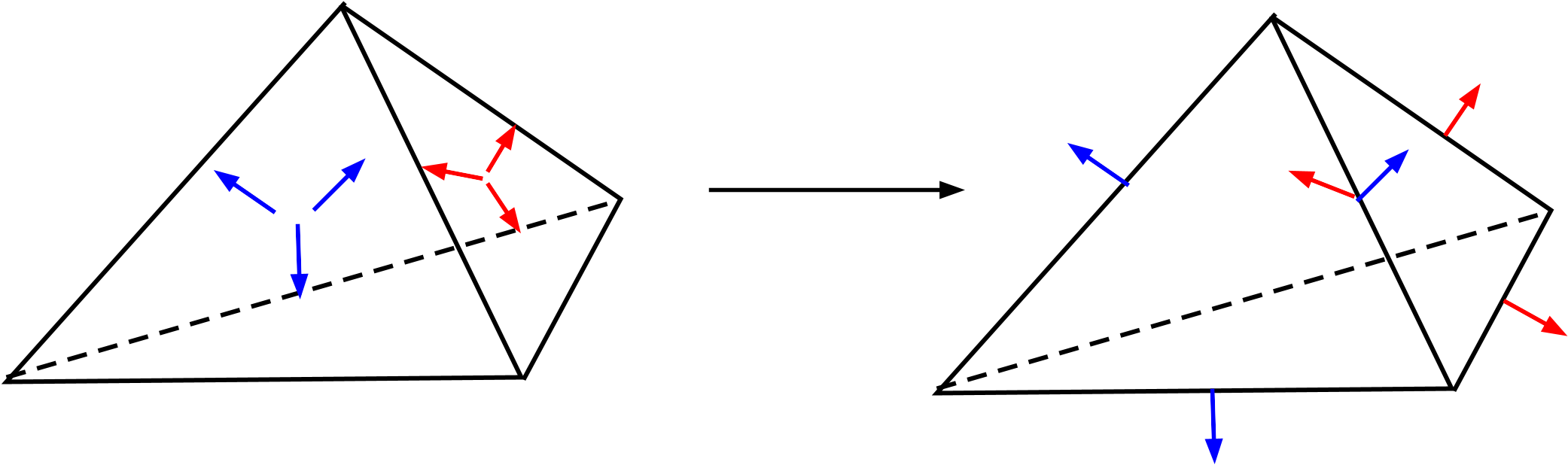
Figure 10. An illustration for the construction of the Hu-Lin-Zhang traceless element. Here, we move the face degrees of freedom to each edge.

Recall that $\iota_{\sigma}^{*}\jmath_{\sigma}^{*}$ maps $C^{\infty}\otimes\mathrm{Alt}^{k,\ell}(\mathbb{R}^{n})$ to $C^{\infty}(\sigma)\otimes\mathrm{Alt}^{k}(\sigma)\otimes\mathrm{Alt}^{\ell-k}(\sigma^{\perp})$, which is a vector bundle on $\sigma$. Correspondingly, we use $\langle\cdot,\cdot\rangle$ to denote an inner product on the vector bundles. This means that $\langle\iota_{\sigma}^{*}\jmath_{\sigma}^{*}w,b\rangle_{\sigma}$, for $w\in C^{\infty}\otimes\mathrm{Alt}^{k,\ell}(\mathbb{R}^{n})$ and $b\in\mathrm{Alt}^{k}(\sigma)\otimes\mathrm{Alt}^{\ell-k}(\sigma^{\perp})$ first takes a pointwise inner product of $\iota_{\sigma}^{*}\jmath_{\sigma}^{*}w$ and $b$, and integrate on the $k$-dimensional cell $\sigma$ (rather than in the $n$-dimensional space).

Proposition 4.4.

The degrees of freedom

(4.10) $$\begin{cases}\langle\iota^{*}_{\sigma}\jmath^{*}_{\sigma}\omega,b\rangle_{\sigma},&\forall~~b\in\mathrm{Alt}^{k}(\sigma)\otimes\mathrm{Alt}^{\ell-k}(\sigma^{\perp}),\quad\dim\sigma=k\\ \langle\iota^{*}_{\sigma}\iota^{*}_{\sigma}\omega,b\rangle_{\sigma},&\forall~~b\in\mathcal{B}^{-}\mathrm{Alt}^{k,\ell}(\sigma),\quad\dim\sigma>\ell\end{cases}$$

for each $\sigma\in\mathcal{T}(K)$ are unisolvent with respect to the shape function space $\mathcal{P}^{-}\mathrm{Alt}^{k,\ell}(K)$. The resulting finite element space is $\iota^{*}\jmath^{*}$-conforming, and denoted as $C_{\iota^{*}\jmath^{*}}\operatorname{\mathcal{P}}^{-}\mathrm{Alt}^{k,\ell}$.

Proof.

The proof follows from carrying over the unisolvency of (4.7) to (4.10) by counting the number of degrees of freedom. First note that we use the same shape function space $\mathcal{P}^{-}\mathrm{Alt}^{k,\ell}$ as in the case of $C_{\iota^{*}\iota^{*}}\operatorname{\mathcal{P}}^{-}\mathrm{Alt}^{k,\ell}$. For the degrees of freedom, the only difference between (4.10) and (4.7) is those on the simplices of dimension $k$ and $\ell$. The dimension count is done once we show that (4.7) and (4.10) have the same numbers.

For the $\iota^{*}\iota^{*}$-conforming space $C_{\iota^{*}\iota^{*}}\operatorname{\mathcal{P}}^{-}\mathrm{Alt}^{k,\ell}$ , the degrees of freedom on each $\ell$ simplex $\sigma_{\ell}$ has the dimension of

$$\dim\mathcal{B}^{-}\mathrm{Alt}^{k,\ell}(\sigma_{\ell})=\dim\mathcal{P}^{-}\mathrm{Alt}^{k,\ell}(\sigma_{\ell})=\binom{\ell+1}{\ell+1}\binom{\ell+1}{k+1}=\binom{\ell+1}{k+1}.$$

Therefore, the total number of degrees of freedom of (4.7) associated with all $\ell$-dimensional simplices $\mathcal{T}_{\ell}$ is $\displaystyle\binom{n+1}{\ell+1}\binom{\ell+1}{k+1}$.

While for (4.10), the degrees of freedom on each $k$ simplex $\sigma_{k}$ have the dimension $\displaystyle\dim\mathrm{Alt}^{\ell-k}(\sigma_{k}^{\perp})=\binom{n-k}{\ell-k}$. Therefore, the total degrees of freedom of (4.10) at $\mathcal{T}_{k}$ is $\displaystyle\binom{n-k}{\ell-k}\binom{n+1}{k+1}.$ By combinatoric identity, the two numbers are identical.

Now it suffices to verify the unisolvency and conformity. Since the second group in (4.10) also exits in (4.7), it suffices to verify the following: for $w\in\operatorname{\mathcal{P}}^{-}\mathrm{Alt}^{k,\ell}$, if $\langle\iota^{*}_{\sigma}\jmath^{*}_{\sigma}\omega,b\rangle_{\sigma}=0$ for all constant $b$ and $\sigma\in\mathcal{T}_{\ell}$, then for each $F\in\mathcal{T}_{\ell}$, $w_{F}:=\iota_{F}^{*}\iota_{F}^{*}w$ vanishes. In fact, by the above vanishing conditions, it holds that $\iota^{*}_{\sigma}\jmath^{*}_{\sigma}w=0$. By Lemma 3.1, $\iota^{*}_{\sigma}\jmath^{*}_{\sigma}w_{F}=0$. Note that $w_{F}$ is in $\operatorname{\mathcal{P}}^{-}\mathrm{Alt}^{k,\ell}(F)\cong\operatorname{\mathcal{P}}^{-}\mathrm{Alt}^{k}(F)$. Therefore we have $\iota_{\tau}^{*}w_{F}=0$ for all $\tau\in\mathcal{T}_{k}(F)$. By the unisolvency of the Whitney form, it then holds that $w_{F}$. The remaining proof is implied in that of Proposition 4.1. ∎

Example 4.5.

For the $C_{\iota^{*}\iota^{*}}\mathcal{P}^{-}\mathrm{Alt}^{1,2}$ element, the degrees of freedom are face moments against the Raviart-Thomas space (3 per face) plus 6 interior DoFs inside each tetrahedron. Next, we move the degrees of freedom from faces (2-simplices) to edges (1-simplices). Each face has 3 degrees of freedom and has 3 edges. Therefore, on each face we send one degree of freedom to each of its edge; and each edge receives two degrees of freedom in total. This leads to the $C_{\iota^{*}\jmath^{*}}\mathcal{P}^{-}\mathrm{Alt}^{1,2}$ element. The degrees of freedom are the moments of edge tangential-normal components (2 per edge) plus 6 inside each tetrahedron.

Remark 4.3.

Conversely, moving degrees of freedom from lower to higher dimensions will weaken the continuity. This is in general doable. The finite element spaces before and after moving degrees of freedom can be connected by a diagram similar to the construction in the Finite Element System [27], and properties of weakened finite element spaces can be derived from those with stronger continuity. In our case, the $C_{\iota^{*}\iota^{*}}$- and $C_{\iota^{*}\jmath^{*}}$-conforming finite element spaces can be obtained from $C_{\iota^{*}\rho^{*}}\mathcal{P}^{-}\mathrm{Alt}^{k,\ell}$, a tensor product of the standard FEEC space $\mathcal{P}^{-}\mathrm{Alt}^{k}$ and $\mathrm{Alt}^{\ell}$. This provides another perspective for deriving the $C_{\iota^{*}\iota^{*}}$- and $C_{\iota^{*}\jmath^{*}}$-conforming finite element spaces above by weakening finite element differential forms. However, we followed a more explicit construction with bubble functions. This approach will also be more transparent for higher order cases.

For convenience, we call the first set of degrees of freedom in (4.10) (those on dimension $k$) the skeletal part and the second set (those on dimensions $>\ell$) the bubble part. Note that for $\sigma\in\mathcal{T}_{\ell}$, it holds that $\mathcal{B}^{-}{\mathbb{W}}^{k,\ell}(\sigma)=\mathcal{P}^{-}\mathrm{Alt}^{k,\ell}(\sigma)$. Therefore, we can also move the degrees of freedom to obtain the $C_{\iota^{*}\jmath^{*}}$-continuity. See the following proposition for a precise statement.

Proposition 4.5.

If $k\leq\ell$, then the degrees of freedom

$$\begin{cases}\langle\iota^{*}_{\sigma}\jmath^{*}_{\sigma}\omega,b\rangle_{\sigma},&\forall~~b\in\mathrm{Alt}^{k}\otimes\mathrm{Alt}^{\ell-k}(\sigma^{\perp}),\quad\dim\sigma=k\\ \langle\iota^{*}_{\sigma}\iota^{*}_{\sigma}\omega,b\rangle_{\sigma},&\forall~~b\in\mathcal{B}^{-}{\mathbb{W}}^{k,\ell}(\sigma),\quad\dim\sigma>\ell\end{cases}$$

are unisolvent for $\operatorname{\mathcal{P}}^{-}{\mathbb{W}}^{k,\ell}$. The resulting finite element space is $\iota^{*}\jmath^{*}$-conforming, denoted as $C_{\iota^{*}\jmath^{*}}\operatorname{\mathcal{P}}^{-}{\mathbb{W}}^{k,\ell}$.

Example 4.6.

As a special case, $C_{\iota^{*}\jmath^{*}}\mathcal{P}^{-}\mathrm{Alt}^{0,\ell}$ gives $\mathrm{Alt}^{\ell}$-valued Lagrange space ($\binom{n}{\ell}$ copies of the scalar Lagrange finite element spaces). Moreover, $C_{\iota^{*}\iota^{*}}\mathcal{P}^{-}\mathrm{Alt}^{k,n}$ gives the discontinuous space $C^{-1}\mathcal{P}^{-}\mathrm{Alt}^{k}$.

Example 4.7.

We discuss some nontrivial examples involving symmetries. Again, we consider the symmetric (1,2)-form in three dimensions. The shape function space is then $\mathbb{W}^{1,1}+\kappa\mathbb{W}^{2,2}=\mathbb{T}+\bm{x}\times\mathbb{S}$, which is traceless. For the $C_{\iota^{*}\iota^{*}}\mathcal{P}^{-}\mathbb{W}^{1,2}$ element with $\iota^{*}\iota^{*}$-conformity, the degrees of freedom are moments against face Raviart-Thomas spaces (3 per face) and 2 inside the cell. Note that the reduction only occurs for the interior degrees of freedom. Next, we move the degrees of freedom from faces to edges. For the $C_{\iota^{*}\jmath^{*}}\mathcal{P}^{-}{\mathbb{W}}^{1,2}$ element, the degrees of freedom are evaluation of the edge tangential-normal components (2 per edge) and 2 inside the tetrahedron. This gives the Hu-Lin-Zhang traceless element in [42]. See Figure 10 for the moving the degrees of freedom step, and Figure 6 for the whole procedure.

4.4. $\iota^{*}\jmath_{[p]}^{*}$-conforming finite elements

In this section, we discuss the $\iota^{*}\jmath_{[p]}^{*}$-conforming finite elements In $\mathcal{T}_{\leq\ell+p-1}$, we require that $\iota^{*}\jmath^{*}_{[p]}$ is single-valued, while in $\mathcal{T}_{\geq\ell+p}$, we require that $\iota^{*}\iota^{*}w$ is single-valued. Note that $\jmath^{*}_{F,[p]}$ is a direct sum of $p$ terms: $\vartheta_{F,\dim F}^{\ast}$, $\vartheta_{F,\dim F-1}^{\ast}$, $\cdots$, $\vartheta_{F,\dim F-p+1}^{\ast}$. When $\dim F=k$, the range of $\vartheta_{F,\dim F-s}^{\ast}$ is in $C^{\infty}(F)\otimes\mathrm{Alt}^{k-s}(F)\otimes\mathrm{Alt}^{\ell-k+s}(F^{\perp}).$

We first assume that $k<\ell$, where the degrees of freedom of the finite element space $C_{\iota^{*}\iota^{*}}\mathcal{P}^{-}\mathrm{Alt}^{k,\ell}$ are located on the simplices of dimensions greater than or equal to $\ell$, $\mathcal{T}_{\ell},\mathcal{T}_{\ell+1},\cdots.$ To impose the $\iota^{*}\jmath_{[p]}^{*}$-conformity, we move the degrees of freedom on simplices of dimension $\ell,\ell+1,\cdots,\ell+p-1$ to $k$-simplices $\sigma$. The new degrees of freedom on $\sigma$ gained from those on $\mathcal{T}_{\ell+s}$ will ensure that the generalized trace $\iota^{\ast}\vartheta_{\sigma,k-s}^{*}$ is single-valued on $\sigma$. To see this is possible, we first check that the number of degrees of freedom matches, i.e., the number of degrees of freedom on $\mathcal{T}_{\ell+s}$ before the move is the same as the number of those new degrees of freedom on $\sigma$ ensuring the $\iota^{\ast}\vartheta_{\sigma,k-s}^{*}$-conformity for all $\sigma$ of dimension $k$. In fact, for each $(\ell+s)$-simplex $F$, the degrees of freedom before the move are inner product against $\mathcal{B}^{-}\mathrm{Alt}^{k,\ell}(F)$. By Lemma 4.1, forms in $\mathcal{B}^{-}\mathrm{Alt}^{k,\ell}(F)$ have the following decomposition: $\mathcal{B}^{-}\mathrm{Alt}^{k,\ell}(F)=\sum\phi_{\sigma}\otimes N^{\ell}(\sigma,F)$. Recall that the dimension of $N^{\ell}(\sigma,F)$ is $\binom{k}{\ell+k-\ell-s}=\binom{k}{k-s}.$ This number coincides with the dimension of $\mathrm{Alt}^{k-s}(\sigma)$. The number of possible $\sigma$ in the decomposition $\sum\phi_{\sigma}\otimes N^{\ell}(\sigma,F)$ (with $F:\dim F=\ell+s$ and $\sigma\trianglelefteq F$) is $\binom{n-k}{\ell-k+s}=\dim\mathrm{Alt}^{\ell-k+s}(\sigma^{\perp})$. Therefore

$$\sum_{\begin{subarray}{c}F:\sigma\trianglelefteq F\\ \dim\sigma=k\end{subarray}}\dim\phi_{\sigma}\otimes N^{\ell}(\sigma,F)=\binom{n-k}{\ell-k+s}\binom{k}{k-s}=\dim(\mathrm{Alt}^{k-s}(\sigma)\otimes\mathrm{Alt}^{\ell-k+s}(\sigma^{\perp})).$$

Summing over all $\sigma$, we have

$$\sum_{F:\dim F=\ell+s}\dim\mathcal{B}^{-}\mathrm{Alt}^{k,\ell}(F)=\sum_{\sigma:\dim\sigma=k}\dim(\mathrm{Alt}^{k-s}(\sigma)\otimes\mathrm{Alt}^{\ell-k+s}(\sigma^{\perp})),$$

for each $s$, where the left hand side is the number of removed degrees of freedom in the process, and the right hand side is the number of new degrees of freedom added on $k$-simplices. The equality therefore shows that the operation does not change the total number of degrees of freedom in an $n$-simplex. See Figure 11 for an illustration.

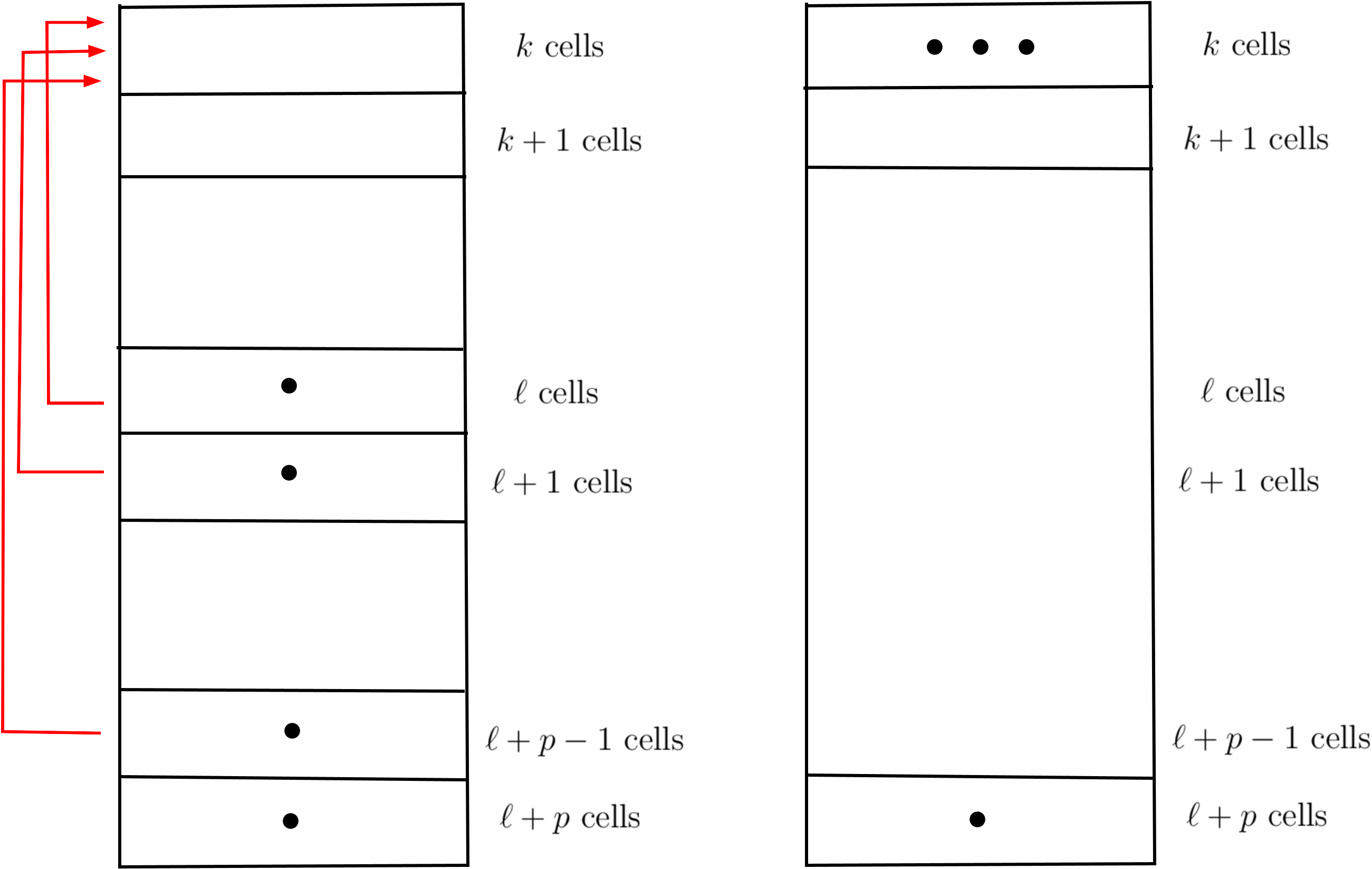
Figure 11. An illustration for moving the degrees of freedom for the $\jmath_{[p]}^{*}$ case. Here, we move the degrees of freedom from $\ell$-, $(\ell+1)$-, …. $(\ell+p-1)$- faces to $k$-faces.

Proposition 4.6.

The degrees of freedom

(4.11) $$\begin{cases}\langle\iota^{*}_{\sigma}\vartheta^{*}_{\sigma,k}\omega,b\rangle_{\sigma},&\forall~~b\in\mathrm{Alt}^{k}(\sigma)\otimes\mathrm{Alt}^{\ell-k}(\sigma^{\perp}),\quad\dim\sigma=k\\ \langle\iota^{*}_{\sigma}\vartheta^{*}_{\sigma,k-1}\omega,b\rangle_{\sigma},&\forall~~b\in\mathrm{Alt}^{k-1}(\sigma)\otimes\mathrm{Alt}^{\ell-k+1}(\sigma^{\perp}),\quad\dim\sigma=k\\ \langle\iota^{*}_{\sigma}\vartheta^{*}_{\sigma,k-2}\omega,b\rangle_{\sigma},&\forall~~b\in\mathrm{Alt}^{k-2}(\sigma)\otimes\mathrm{Alt}^{\ell-k+2}(\sigma^{\perp}),\quad\dim\sigma=k\\ \cdots\\ \langle\iota^{*}_{\sigma}\vartheta^{*}_{\sigma,k-p+1}\omega,b\rangle_{\sigma},&\forall~~b\in\mathrm{Alt}^{k-p+1}(\sigma)\otimes\mathrm{Alt}^{\ell-k+p-1}(\sigma^{\perp}),\quad\dim\sigma=k\\ \langle\iota^{*}_{\sigma}\iota^{*}_{\sigma}\omega,b\rangle_{\sigma},&\forall~~b\in\mathcal{B}^{-}\mathrm{Alt}^{k,\ell}(\sigma),\quad\dim\sigma\geq\ell+p\end{cases}$$

or written in a compact form:

$$\begin{cases}\langle\iota^{*}_{\sigma}\jmath^{*}_{\sigma,[p]}\omega,b\rangle_{\sigma},&\forall~~b\in\bigoplus_{s=0}^{p-1}\mathrm{Alt}^{k-s}(\sigma)\otimes\mathrm{Alt}^{\ell-k+s}(\sigma^{\perp}),\quad\dim\sigma=k\\ \langle\iota^{*}_{\sigma}\iota^{*}_{\sigma}\omega,b\rangle_{\sigma},&\forall~~b\in\mathcal{B}^{-}\mathrm{Alt}^{k,\ell}(\sigma),\quad\dim\sigma\geq\ell+p\end{cases}$$

are unisolvent with respect to the shape function space $\mathcal{P}^{-}\mathrm{Alt}^{k,\ell}(K)$. The resulting finite element space is $\iota^{*}\jmath^{*}_{[p]}$-conforming.

Proof.

We have verified that moving degrees of freedom as described above does not change the total number of degrees of freedom. Therefore, it suffices to show the unisolvency and conformity.

Suppose that all the degrees of freedom in $\mathcal{T}_{k}$ vanish on $w\in\mathcal{P}^{-}\mathrm{Alt}^{k,\ell}$. It suffices to show that $\iota_{F}^{*}\iota_{F}^{*}w=0$ for any $F\in\mathcal{T}_{\ell+p-1}$. Then, by the last set of degrees of freedom, we can conclude with the unisolvency. Fix $F\in\mathcal{T}_{\ell+p-1}$ and let $w_{F}=\iota_{F}^{*}\iota_{F}^{*}w\in\mathcal{P}^{-}\mathrm{Alt}^{k,\ell}(F)$. By Lemma 3.1, it holds that $\iota_{E}^{*}\jmath_{E,[p]}^{*}w_{F}=0$ for all $E\in\mathcal{T}_{k}$. Note that $w_{F}$ is in $\mathbb{R}^{\ell+p-1}$, therefore, by Lemma 3.2, it holds that $\jmath_{E,[p]}^{*}=\rho_{E}^{*}$. Therefore, it then conclude that $w_{F}=0$. ∎

Remark 4.4.

The situation is slightly different for the case when $\ell\leq k\leq\ell+p-1$. In this case, the degrees of freedom of the finite element $C_{\iota^{*}\iota^{*}}\mathcal{P}^{-}\mathrm{Alt}^{k,\ell}$ are only located on $\mathcal{T}_{k},\mathcal{T}_{k+1},\cdots$. Therefore, we only move the degrees of freedom $\mathcal{T}_{k},\mathcal{T}_{k+1},\cdots\mathcal{T}_{\ell+p-1}$ to those involving $\vartheta_{\sigma,\ell}^{\ast}$, $\vartheta^{\ast}_{\sigma,\ell-1}$, $\cdots$, $\vartheta^{\ast}_{\sigma,k-p+1}$ on $\mathcal{T}_{k}$, respectively. This is also reflected in the degrees of freedom (4.11) by the fact that $\vartheta_{\sigma,k}^{*},\cdots\vartheta_{\sigma,\ell+1}^{*}$ vanish when $\ell\leq k$.

Example 4.8.

A trivial case is that when $\jmath_{[p]}^{*}=\rho^{*}$ (which holds for sufficiently large $p$; see Lemma 3.2). In this case, the construction gives $C_{\iota^{*}}\mathcal{P}^{-}\mathrm{Alt}^{k}\otimes\mathrm{Alt}^{\ell}$, i.e., alternating $\ell$-forms-valued finite element $k$-forms $C_{\iota^{*}}\mathcal{P}^{-}\mathrm{Alt}^{k}$ [3, 5].

Similar to the $\iota^{*}\jmath^{*}$-conforming finite element space, the degrees of freedom in $\mathcal{T}_{<\ell+p}$ are not changed in the symmetry reduction (see Remark 4.2). This indicates that the process of moving the degrees of freedom can be also done from $C_{\iota^{\ast}\iota^{\ast}}\mathcal{P}^{-}{\mathbb{W}}_{[p]}^{k,\ell}$ to $C_{\iota^{\ast}\jmath^{\ast}_{[p]}}\mathcal{P}^{-}{\mathbb{W}}_{[p]}^{k,\ell}$.

Proposition 4.7.

If $k\leq\ell+p-1$, then the degrees of freedom

(4.12) $$\begin{cases}\langle\iota^{*}_{\sigma}\vartheta^{*}_{\sigma,k}\omega,b\rangle_{\sigma},&\forall~~b\in\mathrm{Alt}^{k}(\sigma)\otimes\mathrm{Alt}^{\ell-k}(\sigma^{\perp}),\quad\dim\sigma=k\\ \langle\iota^{*}_{\sigma}\vartheta^{*}_{\sigma,k-1}\omega,b\rangle_{\sigma},&\forall~~b\in\mathrm{Alt}^{k-1}(\sigma)\otimes\mathrm{Alt}^{\ell-k+1}(\sigma^{\perp}),\quad\dim\sigma=k\\ \langle\iota^{*}_{\sigma}\vartheta^{*}_{\sigma,k-2}\omega,b\rangle_{\sigma},&\forall~~b\in\mathrm{Alt}^{k-2}(\sigma)\otimes\mathrm{Alt}^{\ell-k+2}(\sigma^{\perp}),\quad\dim\sigma=k\\ \cdots\\ \langle\iota^{*}_{\sigma}\vartheta^{*}_{\sigma,k-p+1}\omega,b\rangle_{\sigma},&\forall~~b\in\mathrm{Alt}^{k-p+1}(\sigma)\otimes\mathrm{Alt}^{\ell-k+p-1}(\sigma^{\perp}),\quad\dim\sigma=k\\ \langle\iota^{*}_{\sigma}\iota^{*}_{\sigma}\omega,b\rangle_{\sigma},&\forall~~b\in\mathcal{B}^{-}{\mathbb{W}}_{[p]}^{k,\ell}(\sigma),\quad\dim\sigma\geq\ell+p\end{cases}$$

or written compactly,

$$\begin{cases}\langle\iota^{*}_{\sigma}\jmath^{*}_{\sigma,[p]}\omega,b\rangle_{\sigma},&\forall~~b\in\bigoplus_{s=0}^{p-1}\mathrm{Alt}^{k-s}(\sigma)\otimes\mathrm{Alt}^{\ell-k+s}(\sigma^{\perp}),\quad\dim\sigma=k\\ \langle\iota^{*}_{\sigma}\iota^{*}_{\sigma}\omega,b\rangle_{\sigma},&\forall~~b\in\mathcal{B}^{-}{\mathbb{W}}^{k,\ell}_{[p]}(\sigma),\quad\dim\sigma\geq\ell+p\end{cases}$$

are unisolvent for $C_{\iota^{\ast}\jmath^{\ast}_{[p]}}\mathcal{P}^{-}{\mathbb{W}}_{[p]}^{k,\ell}$. The resulting finite element space is $\iota^{*}\jmath_{[p]}^{*}$-conforming.

Remark 4.5.

It is also possible to construct the finite element space $C_{\iota^{*}\jmath_{[q]}^{*}}\mathcal{P}^{-}{\mathbb{W}}_{[p]}^{k,\ell}$ whenever $q\leq p$.

Example 4.9.

The resulting finite elements in three space dimensions all exist in the literature. Namely, for $p\geq 2$, one of the case in Lemma 3.2 holds. See the following examples:

1. For $\mathrm{Alt}^{1,1}$, it holds that $\jmath_{e,[p]}^{*}=\rho^{*}$ for $p\geq 2$. Therefore, the construction gives three copies of the Nédélec elements.

2. For $\mathrm{Alt}^{2,2}$, it holds that $\jmath_{f,[p]}^{*}=\rho^{*}$ for $p\geq 2$. Therefore, the construction gives three copies of the Raviart-Thomas elements.

3. For $\mathrm{Alt}^{1,2}$, it holds that $\jmath_{e,[p]}^{*}=\rho^{*}$ for $p\geq 2$. Therefore, the construction gives three copies of the Nédélec element.

4. For $\mathrm{Alt}^{2,1}$, we can consider the construction when $p\geq 2$. For $p=2$, $\jmath_{f,[2]}^{*}=\iota^{*}$, while for the other cases, $\jmath_{f,[p]}^{*}=\rho^{*}$. The latter always gives three copies of the Raviart-Thomas element.

We will see some nontrivial $\iota^{*}\jmath_{[p]}^{*}$-conforming finite elements in four dimensions in Section 5.2.

5. Tensorial Whitney forms: examples and complexes

In this section, we provide some examples of tensorial Whitney forms constructed in the previous section. Recall that we have constructed

1. $C_{\iota^{*}\iota^{*}}\mathcal{P}^{-}\mathrm{Alt}^{k,\ell}$ for $k\leq\ell$;

2. $C_{\iota^{*}\iota^{*}}\mathcal{P}^{-}{\mathbb{W}}^{k,\ell}$ for $k\leq\ell$;

3. $C_{\iota^{*}\jmath^{*}}\mathcal{P}^{-}\mathrm{Alt}^{k,\ell}$ for $k\leq\ell$;

4. $C_{\iota^{*}\jmath^{*}}\mathcal{P}^{-}{\mathbb{W}}^{k,\ell}$ for $k\leq\ell$.
   For the iterated constructions, we have

5. $C_{\iota^{*}\iota^{*}}\mathcal{P}^{-}{\mathbb{W}}^{k,\ell}_{[p]}$ for $k\leq\ell+p-1$;

6. $C_{\iota^{*}\jmath^{*}_{[p]}}\mathcal{P}^{-}{\mathbb{W}}^{k,\ell}_{[p]}$ for $k\leq\ell+p-1$.

The spaces of symmetries (2)(4)(6) are candidates for discrete BGG complexes.

In subsequent sections, we first provide a summary for the examples in three space dimensions. It should be noted that the pattern presented in two and three dimensions are deceptive, leading to some challenge to generalize the idea to higher dimensions,. In general dimensions, we demonstrate the families of the $(k,k)$ forms to investigate the general pattern and the nontriviality in higher dimensions. Finally, we show candidates of finite element and distributional BGG complexes, and show that a necessary dimension condition for correct cohomology holds.

5.1. Recap in three dimensions

In this subsection, we summarize the finite elements in three dimensions. For simplicity, here we only list the symmetric version $C_{\iota^{*}\iota^{*}}\mathcal{P}^{-}{\mathbb{W}}_{[p]}^{k,\ell}$ and $C_{\iota^{*}\jmath_{[p]}^{*}}\mathcal{P}^{-}{\mathbb{W}}_{[p]}^{k,\ell}$.

	0	1	2	3
0	Lagrange	first type Nédélec	RT	DG
1	second type Nédélec	full Regge $\mathbb{M}+\bm{x}\times\mathbb{M}$	full MCS $\mathbb{M}+\bm{x}\mathbb{V}$	$(\mathrm{DG})^{3}$
		Figure 5 (I)	Figure 7 (I)
2	BDM	$\mathrm{full~MCS}^{\top}C_{tn}$ $\mathbb{M}+\bm{x}\times\mathbb{M}$	full HHJ $\mathbb{M}+\bm{x}\mathbb{V}$	$(\mathrm{DG})^{3}$
	Figure 5 (II)	Figure 6 (I)	Figure 8 (I)
3	$\mathrm{DG}_{1}$	$C^{-1}\mathrm{Ned}$	$C^{-1}\mathrm{RT}$	DG
	Figures 6 and 7 (II)	Figure 8 (II)

Table 7. $C_{\iota^{*}\iota^{*}}\mathcal{P}^{-}\mathrm{Alt}^{k,\ell}$

	0	1	2	3
0	Lagrange	-	-	-
1	second type Nédélec	Regge $\mathbb{S}$	-	-
		(Figure 5 (I-II))
2	BDM	$\mathrm{MCS}^{\top}$ face $C_{tn}$ traceless $\mathbb{T}+\bm{x}\times\mathbb{S}$	HHJ $\mathbb{S}$	-
		(Figure 6 (I-II))	(Figure 5 (I-II))
3	$C^{-1}\mathcal{P}_{1}$	$C^{-1}\mathrm{Ned}$	$C^{-1}\mathrm{RT}$	DG

Table 8. $C_{\iota^{*}\iota^{*}}\mathcal{P}^{-}{\mathbb{W}}^{k,\ell}$

	0	1	2	3
0	Lagrange	first type Nédélec	-	-
1	second type Nédélec	full Regge $\mathbb{M}+\bm{x}\times\mathbb{M}$	MCS $\mathbb{T}$ (Figure 7 (I-II))	-
2	BDM	$\mathrm{MCS}^{\top}$ $\mathbb{M}+\bm{x}\times\mathbb{M}$	full HHJ $\mathbb{M}+\bm{x}\mathbb{V}$	$\mathrm{(DG)}^{3}$
3	$C^{-1}\mathcal{P}_{1}$	$C^{-1}\mathrm{Ned}$	$C^{-1}\mathrm{RT}$	DG

Table 9. $C_{\iota^{*}\iota^{*}}\mathcal{P}^{-}{\mathbb{W}}_{[2]}^{k,\ell}$

	0	1	2	3
0	Lagrange	-	-	-
1	vector Lagrange	Regge $\mathbb{S}$	-	-
2	vector Lagrange	HLZ $\mathbb{T}+\bm{x}\times\mathbb{S}$ (Figure 6, rightmost)	HHJ $\mathbb{S}$	-
3	Lagrange	Nédélec	RT	DG

Table 10. $C_{\iota^{*}\jmath^{*}}\mathcal{P}^{-}{\mathbb{W}}^{k,\ell}$

	0	1	2	3
0	Lagrange	first type Nédélec	-	-
1	vector Lagrange	vector Nédélec	MCS $\mathbb{T}$	-
2	vector Lagrange	vector Nédélec	vector RT	$\mathrm{(DG)}^{3}$
3	Lagrange	Nédélec	RT	DG

Table 11. $C_{\iota^{*}\jmath_{[2]}^{*}}\mathcal{P}^{-}{\mathbb{W}}_{[2]}^{k,\ell}$

5.2. $(k,k)$ forms

In this section, we consider the $(k,k)$ forms in general dimensions, especially for $k=1,2,3.$ Specifically, we consider

1. $C_{\iota^{*}\iota^{*}}\mathcal{P}^{-}\mathrm{Alt}^{k,k}$, and its reduction $C_{\iota^{*}\iota^{*}}\mathcal{P}^{-}{\mathbb{W}}_{[p]}^{k,k}$. The most interesting case is $p=1$, where the local shape function space is $\mathcal{P}^{-}{\mathbb{W}}^{k,k}={\mathbb{W}}^{k,k}$.

2. $C_{\iota^{*}\jmath_{[p]}^{*}}\mathcal{P}^{-}\mathrm{Alt}^{k,k}$. This gives some nontrivial case for $\iota^{*}\jmath_{[p]}^{*}$-conforming space whose continuity lies between $\iota^{*}\iota^{*}$ and $\iota^{*}\rho^{*}$.

By (4.6), no degrees of freedom are put on any $\sigma\in\mathcal{T}_{>2k}$ for $\mathcal{P}^{-}\operatorname{Alt}^{k,\ell}$, while for $\sigma\in\mathcal{T}_{2k}$, the numbers of the degrees of freedom are $\binom{2k+1}{k+1}$. In the symmetric case, the shape function space of $\mathcal{P}^{-}\mathbb{W}^{k,k}$ is constant $\mathbb{W}^{k,k}$. The symmetry reduction removes the degrees of freedom of $\mathcal{P}^{-}\mathrm{Alt}^{k-1,k+1}$ from those of $\mathcal{P}^{-}\mathrm{Alt}^{k,k}$. For $\mathcal{P}^{-}\mathrm{Alt}^{k-1,k+1}$, no degrees of freedom are put for $\sigma\in\mathcal{T}_{>2k}$, while for $\sigma\in\mathcal{T}_{2k}$, the numbers of degrees of freedom are $\binom{2k+1}{k}$. Removing these numbers from the dimension count of $\mathcal{P}^{-}\mathrm{Alt}^{k,k}$, we get the following.

Corollary 5.1.

For $\mathcal{P}^{-}\mathbb{W}^{k,k}=\mathbb{W}^{k,k}$ finite element with $\iota^{*}\iota^{*}$-conformity, there are no degrees of freedom on $\sigma\in\mathcal{T}_{\geq 2k}$.

Consequently, the degrees of freedom for $\mathcal{P}^{-}\mathrm{Alt}^{k,k}$ are

(5.1) $$\langle\iota^{*}_{\sigma}\iota^{*}_{\sigma}\omega,b\rangle_{\sigma},\qquad\forall~~b\in\mathcal{B}^{-}\mathrm{Alt}^{k,k}(\sigma),\forall\sigma\in\mathcal{T}_{[k,2k]},$$

while for $\mathcal{P}^{-}\mathbb{W}^{k,k}$ the degrees of freedom are

(5.2) $$\langle\iota^{*}_{\sigma}\iota^{*}_{\sigma}\omega,b\rangle_{\sigma},\qquad\forall~~b\in\mathcal{B}^{-}\mathbb{W}^{k,k}(\sigma),\forall\sigma\in\mathcal{T}_{[k,2k-1]}.$$

Recall that $\mathcal{T}_{[k,2k]}:\mathcal{T}_{\geq k}\cap\mathcal{T}_{\leq 2k}$ denotes the simplices with dimension in $[k,2k]$. Here $\mathcal{B}^{-}\mathbb{W}^{k,k}(\sigma)=\mathcal{B}^{-}\mathrm{Alt}^{k,k}(\sigma)\cap\mathcal{N}(\mathcal{S}_{\dagger}^{k,k})=\mathbb{W}^{k,k}(\sigma)\cap\bigcap_{F:\operatorname{codim}(F)=1}\mathcal{N}(\iota_{F}^{*}\iota_{F}^{*})$.

For $k=1$, this result covers the Regge element. In any space dimension, $\mathcal{P}^{-}\mathrm{Alt}^{1,1}$ has one degree of freedom (DoF) per edge and three DoFs per 2-faces.

The symmetry reduction completely removes the face DoFs (3-3=0), and thus we obtain the symmetric Regge element. The dimension count is summarized in Table 15.

$n$	1	2	$\geq 3$
DoFs on $n$-face of $\mathcal{P}^{-}\mathrm{Alt}^{1,1}$	1	3	0
DoFs on $n$-face of $\mathcal{P}^{-}\mathrm{Alt}^{0,2}$	0	3	0
DoFs on $n$-face of $\mathcal{P}^{-}\mathbb{W}^{1,1}$	1	0	0

Table 12. The dimension count involved in the construction of $\mathcal{P}^{-}\mathrm{Alt}^{1,1}$ and $\mathcal{P}^{-}{\mathbb{W}}^{1,1}$. Here the continuity is $C_{\iota^{*}\iota^{*}}$. Here, we highlight the dimension (in blue) that the degrees of freedom are totally modified due to symmetric reduction. The numbers in the last row are obtained from the second row minus the first row.

For $k=2$, we obtain the shape functions and degrees of freedom of $\mathcal{P}^{-}\mathrm{Alt}^{2,2}$ and $\mathcal{P}^{-}\mathbb{W}^{2,2}=\mathbb{W}^{2,2}$ by a similar argument. The dimension count is summarized in Table 16.

$n$	1	2	3	4	$\geq 5$
DoFs on $n$-face of $\mathcal{P}^{-}\mathrm{Alt}^{2,2}$	0	1	8	10	0
DoFs on $n$-face of $\mathcal{P}^{-}\mathrm{Alt}^{1,3}$	0	0	6	10	0
DoFs on $n$-face of $\mathcal{P}^{-}\mathbb{W}^{2,2}$	0	1	2	0	0
DoFs on $n$-face of $\mathcal{P}^{-}\mathrm{Alt}^{0,4}$	0	0	0	5	0
DoFs on $n$-face of $\mathcal{P}^{-}{\mathbb{W}}^{2,2}_{[2]}$	0	1	8	5	0

Table 13. The dimension count involved in the construction of $\mathcal{P}^{-}\mathrm{Alt}^{2,2}$ and $\mathcal{P}^{-}{\mathbb{W}}^{2,2}_{[p]}$. Here the continuity is $C_{\iota^{*}\iota^{*}}$. We highlight in blue the number of DoFs after the symmetry reduction.

The case with $k=3$ is summarized in Table 17.

$n$	1	2	3	4	5	6	$\geq 7$
DoFs on $n$-face of $\mathcal{P}^{-}\mathrm{Alt}^{3,3}$	0	0	1	15	45	35	0
DoFs on $n$-face of $\mathcal{P}^{-}\mathrm{Alt}^{2,4}$	0	0	0	10	40	35	0
DoFs on $n$-face of $\mathcal{P}^{-}\mathbb{W}^{3,3}$	0	0	1	5	5	0	0
DoFs on $n$-face of $\mathcal{P}^{-}\mathrm{Alt}^{1,5}$	0	0	0	0	15	21	0
DoFs on $n$-face of $\mathcal{P}^{-}{\mathbb{W}}^{3,3}_{[2]}$	0	0	1	15	30	14	0
DoFs on $n$-face of $\mathcal{P}^{-}\mathrm{Alt}^{0,6}$	0	0	0	0	0	7	0
DoFs on $n$-face of $\mathcal{P}^{-}{\mathbb{W}}^{3,3}_{[3]}$	0	0	1	15	45	28	0

Table 14. The dimension count involved in the construction of $\mathcal{P}^{-}\mathrm{Alt}^{3,3}$ and $\mathcal{P}^{-}{\mathbb{W}}^{3,3}_{[p]}$. Here the continuity is $C_{\iota^{*}\iota^{*}}$. We highlight in blue the number of DoFs after the symmetry reduction.

Next, we show how to move the degrees of freedom to obtain $\iota^{*}\jmath_{[p]}^{*}$-conforming space for $p\geq 2$. We begin by (1,1) form.

• For $\mathrm{Alt}^{1,1}$, we can move the degree of freedom from 2-faces to 1-faces. Each 2-face has three degrees of freedom, and 3 edges. Therefore, each 2-face sends 1 degrees of freedom to one of its edge, and each edge receives $(n-1)$ degrees of freedom in total.

  $n$	1	2	$\geq 3$
  DoFs on $n$-face for $p=1$	1	3	0
  DoFs on $n$-face for $p=2$	$n$	0	0

  Table 15. The dimension count involved in the construction of $\mathcal{P}^{-}\mathrm{Alt}^{1,1}$

Next, we consider (2,2) form in four dimensions.

• For $p=2$, we move the degrees of freedom from 3-faces to 2-faces. Each face has 8 degrees of freedom and four 2-faces. Therefore, each 3-face sends 2 of its degrees of freedom to one of 2-face, and each 2-face receives 4 in total. Therefore, the construction of $C_{\iota^{*}\jmath_{[2]}^{*}}\mathrm{Alt}^{2,2}$ has 5 degrees of freedom in each 2-face. Suppose that the 2-face is parallel to the plane spanned by $x_{1}$ and $x_{2}$. Then the $\iota^{*}\iota^{*}$ trace corresponds to $dx^{1}\wedge dx^{2}$, while $\iota^{*}\jmath_{[2]}^{*}$ trace corresponds to $dx^{1}\wedge dx^{2}$, $dx^{1}\wedge dx^{3}$, $dx^{1}\wedge dx^{4}$, $dx^{2}\wedge dx^{3}$, $dx^{2}\wedge dx^{4}$.

• For $p=3$, we continue moving the degrees of freedom from 4-faces to 2-faces. Each 4 face has 10 degrees of freedom and 10 2-faces. Therefore, each 2-face receives 1 degrees of freedom. The construction then has 6 degrees of freedom in each 2-face. Clearly, the result is $\iota^{*}\rho^{*}$-conforming.

$n$	1	2	3	4	$\geq 5$
DoF on $n$-face of $C_{\iota^{*}\iota^{*}}\mathcal{P}^{-}\mathrm{Alt}^{2,2}$	0	1	8	10	0
DoF on $n$-face of $C_{\iota^{*}\jmath^{*}_{[2]}}\mathcal{P}^{-}\mathrm{Alt}^{2,2}$	0	5	0	10	0
DoF on $n$-face of $C_{\iota^{*}\jmath^{*}_{[3]}}\mathcal{P}^{-}\mathrm{Alt}^{2,2}$	0	6	0	0	0
DoF on $n$-face of $C_{\iota^{*}\jmath^{*}_{[2]}}\mathcal{P}^{-}{\mathbb{W}}^{2,2}_{[2]}$	0	5	0	5	0

Table 16. The dimension count involved in the construction of $\mathcal{P}^{-}\mathrm{Alt}^{2,2}$ and $\mathcal{P}^{-}{\mathbb{W}}^{2,2}_{[p]}$ in 4 dimensions, with $\iota^{*}\jmath_{[p]}^{*}$-conformity. Here, numbers in blue indicates the number of DoFs after the symmetry reduction; red indicates the DoFs that have been moved to lower dimensional simplices; green indicates the simplices that receive DoFs from higher dimensional cells. The blue slots do not intersect with the red ones.

$n$	1	2	3	4	5	6	$\geq 7$
DoF on $n$-face for $C_{\iota^{*}\iota^{*}}\mathcal{P}^{-}\mathrm{Alt}^{3,3}$	0	0	1	15	45	35	0
DoF on $n$-face for $C_{\iota^{*}\jmath^{*}_{[2]}}\mathcal{P}^{-}\mathrm{Alt}^{3,3}$	0	0	10	0	45	35	0
DoF on $n$-face for $C_{\iota^{*}\jmath^{*}_{[3]}}\mathcal{P}^{-}\mathrm{Alt}^{3,3}$	0	0	19	0	0	35	0
DoF on $n$-face for $C_{\iota^{*}\jmath^{*}_{[4]}}\mathcal{P}^{-}\mathrm{Alt}^{3,3}$	0	0	20	0	0	0	0
DoF on $n$-face of $C_{\iota^{*}\iota^{*}}\mathcal{P}^{-}{\mathbb{W}}^{3,3}_{[2]}$	0	0	1	15	30	14	0
DoF on $n$-face of $C_{\iota^{*}\jmath_{[2]}^{*}}\mathcal{P}^{-}{\mathbb{W}}^{3,3}_{[2]}$	0	0	10	0	30	14	0
DoF on $n$-face of $C_{\iota^{*}\iota^{*}}\mathcal{P}^{-}{\mathbb{W}}^{3,3}_{[3]}$	0	0	1	15	45	28	0
DoF on $n$-face of $C_{\iota^{*}\jmath_{[2]}^{*}}\mathcal{P}^{-}{\mathbb{W}}^{3,3}_{[3]}$	0	0	10	0	45	28	0
DoF on $n$-face of $C_{\iota^{*}\jmath_{[3]}^{*}}\mathcal{P}^{-}{\mathbb{W}}^{3,3}_{[3]}$	0	0	19	0	0	28	0

Table 17. The dimension count involved in the construction of $\mathcal{P}^{-}\mathrm{Alt}^{3,3}$ and $\mathcal{P}^{-}{\mathbb{W}}^{3,3}_{[p]}$ in 6 dimensions, with $\iota^{*}\jmath_{[p]}^{*}$ continuity. Here, numbers in blue indicates the number of DoFs after the symmetry reduction; red indicates the DoFs that have been moved to lower dimensional simplices; green indicates the simplices that receive DoFs from higher dimensional cells. The blue slots do not intersect with the red ones.

5.3. Tensor-valued distributions and complexes

From the pattern in Figure 2, we observe that in 3D, the first part of each complex consists of classical finite elements (piecewise polynomials), while the second part consists of distributions (Dirac deltas). So far we have constructed finite elements which potentially fit in the first part of complexes (the lower triangular part of Figure 2). In this subsection, we introduce the distributional spaces and verify the dimension count in any space dimension, which is a necessary condition for the discrete complexes to have the correct cohomology.

For $k\geq\ell$, we introduce the following $\iota^{*}\jmath^{*}$ distributional spaces:

$$D_{\iota^{*}\jmath^{*}}\mathbb{W}^{k,\ell}:=\operatorname{span}\{\omega\mapsto\langle\iota^{*}\jmath^{*}(\star\star)\omega,b\rangle_{\sigma},\forall~~b\in\mathrm{Alt}^{k-\ell}(\sigma^{\perp}),\sigma\in\mathcal{T}_{n-k}^{\circ}\},$$

where $\star\star:\mathrm{Alt}^{k,\ell}\to\mathrm{Alt}^{n-k,n-\ell}$ is the two-sided Hodge star operator. The distribution above can be regarded as a dual of the skeletal part of $\mathcal{P}^{-}{\mathbb{W}}^{k,\ell}$, while the other degrees of freedom (the bubbles) of $\mathcal{P}^{-}{\mathbb{W}}^{k,\ell}$ do not appear in these distributional spaces.

The complex now reads

(5.3)

More generally, for $k\geq\ell+p-1$, we introduce the following distribution spaces:

$$D_{\iota^{*}\jmath^{*}_{[p]}}\widetilde{\mathbb{W}}^{k,\ell}_{[p]}:=\operatorname{span}\{\omega\mapsto\langle\iota^{*}\jmath^{*}_{[p]}(\star\star)\omega,b\rangle_{\sigma},\forall~~b\in\bigoplus_{s=0}^{p-1}\mathrm{Alt}^{n-k-s}(\sigma)\otimes\mathrm{Alt}^{k-\ell+s}(\sigma^{\perp}),\sigma\in\mathcal{T}_{n-k}^{\circ}\}.$$

Again, the distribution comes from the skeletal part of $\mathcal{P}^{-}{\mathbb{W}}^{k,\ell}_{[p]}$.

Now we can formally write down the BGG complex linking line $\ell$ and $\ell+p$.

(5.4)

We leave the details of the definition of the differential operator to the subsequent paper, but the result of the Euler characteristic (dimension count) is given below.

Theorem 5.1.

Given any triangulation $\mathcal{T}$ of a contractible domain $\Omega$, the Euler characteristic of (5.4) is equal to that of the smooth BGG complex (2.22). That is,

(5.5) $$\sum_{\theta=0}^{\ell+p-1}(-1)^{\theta}\dim C_{\iota^{*}\jmath^{*}_{[p]}}\mathcal{P}^{-}{\mathbb{W}}^{\theta,\ell}_{[p]}+\sum_{\theta=0}^{n-\ell-1}(-1)^{n+p-1}\dim D_{\iota^{*}\jmath^{*}_{[p]}}\widetilde{{\mathbb{W}}}^{n-\theta,\ell+p}_{[p]}=\binom{n}{\ell+p}+(-1)^{p-1}\binom{n}{\ell}.$$

Especially, when $\ell=k+1,p=1$, we obtain that the Euler characteristic of (5.3) is equal to that of (2.4). That is,

(5.6) $$\sum_{\theta=0}^{\ell}(-1)^{\theta}C_{\iota^{*}\jmath^{*}}\mathcal{P}^{-}{\mathbb{W}}^{\theta,\ell}+\sum_{\theta=0}^{n-\ell-1}(-1)^{n}\dim D_{\iota^{*}\jmath^{*}}{\mathbb{W}}^{n-\theta,\ell+1}=\binom{n+1}{\ell+1}.$$

Now we show the examples in three and four dimensions.

5.3.1. Three-dimensional complexes

In three dimensions, we have the following complexes:

1. The discrete Hessian complex (linking row 0 and 1) is

   (5.7)

2. The discrete Regge complex (linking row 1 and 2) is

   (5.8)

3. The discrete divdiv complex (linking row 2 and 3) is

   (5.9)

4. The discrete grad curl complex (linking row 0 and 2) is

   (5.10)

5. The discrete curl div complex (linking row 1 and 3) is

   (5.11)

6. The discrete grad div complex (linking row 0 and 3) is

   (5.12)

5.3.2. Four-dimensional complexes

In four dimensions, we also show the construction of the Hessian complex (for line 0 and 1) and the Regge complex (for line 1 and 2).

To this end, we introduce the following vector proxies. We use $\mathbb{R}$ to represent 0-forms and 4-forms, $\mathbb{V}\cong\mathbb{R}^{4}$ to represent 1-forms and 3-forms, and $\mathbb{K}\cong\mathbb{R}^{6}$ to represent 2-forms, see Example 3.2 and [50] for the de Rham case. In fact, $\mathbb{K}$ can be naturally regarded as a skew-symmetric matrix space in four dimensions. Therefore, we can define the trace $\iota^{*}$ of a $\mathbb{K}$-valued function $\bm{w}$ on any 2-faces by $\bm{t}_{1}\cdot\bm{w}\cdot\bm{t}_{2}$. Note that since $\bm{w}$ is skew-symmetric, the trace is well-defined. Similar to how we use $t$ to represent the relevant quantity for 1-forms and $n$ for 3-forms, we use $m$ to represent the trace in the vector proxies. For convenience, we still use double indices $(i,j)$ to index the components of $\mathbb{K}$.

For $\mathbb{K}$, we define the following operator: $\star:\mathbb{K}\to\mathbb{K}$ such that $[\star a]_{(k,l)}=a_{(i,j)}$ for $\text{sgn}(i,j,k,l)=1$. Further, for $\mathbb{K}\otimes\mathbb{V}$, we define the contraction as $\text{ctr}:\mathbb{K}\otimes\mathbb{V}\to\mathbb{V}$ such that $\text{ctr}(\bm{w}\otimes v)=\bm{w}v$, which is the vector proxy of $\mathcal{S}:\mathrm{Alt}^{2,1}\to\mathrm{Alt}^{3,0}$. We define $\text{ctr}_{\star}:\mathbb{K}\otimes\mathbb{V}\to\mathbb{V}$ by $\text{ctr}_{\star}(\bm{w}\otimes v)=(\star\bm{w})v$, which is the vector proxy of $\mathcal{S}_{\dagger}:\mathrm{Alt}^{2,3}\to\mathrm{Alt}^{1,4}$. Therefore, we can define the contraction free space $\mathbb{CF}$ as the kernel of ctr, which is a subspace of $\mathrm{Alt}^{2,1}\cong\mathbb{K}\otimes\mathbb{V}$. Similarly, we define $\mathbb{CF}_{\star}^{\top}\subseteq\mathrm{Alt}^{3,2}\cong\mathbb{V}\otimes\mathbb{K}$.

Next, we define the transpose $\top:\mathbb{K}\otimes\mathbb{V}\to\mathbb{V}\otimes\mathbb{K}$. Based on this definition, we can then define $\text{ctr}^{\top}$ as the vector proxy of $\mathcal{S}:\mathrm{Alt}^{3,2}\to\mathrm{Alt}^{4,1}$ and $\text{ctr}_{\star}^{\top}$ as the vector proxy of $\mathcal{S}_{\dagger}:\mathrm{Alt}^{1,2}\to\mathrm{Alt}^{0,3}$.

Similarly, we can define the inverse contraction as the adjoint of these contractions. We denote the inverse contractions related to the operators $\star$ and $\top$ as $\text{ictr}_{\star}$ and $\text{ictr}^{\top}$, respectively.

It can be easily checked that $\text{ctr}\circ\text{ictr}=3\text{id}$. Therefore, we can define a projection $\text{cdev}:=\text{id}-\frac{1}{3}\text{ictr}\circ\text{ctr}.$ (contraction deviatoric tensor) to the contraction free space $\mathbb{CF}$. Similarly, we can define the remaining three operators.

With these notations, one can compute (with similar ideas in three dimensions) that the $\mathcal{S}_{\dagger}:\mathrm{Alt}^{2,1}\to\mathrm{Alt}^{1,2}$ is $\bm{A}\mapsto\bm{A}^{\top}-\text{ictr}^{\top}~\text{ctr}\bm{A}$. Note that the formulation in four dimensions resembles that in three dimensions, namely, $\bm{A}\mapsto\bm{A}^{\top}-\operatorname{tr}\bm{A}I$. We highlight that $\mathcal{S}^{2,1}_{\dagger}$ (as well as $\mathcal{S}^{2,1}$) is exactly $\top$ when restricted in $\mathbb{CF}$.

With the above proxies, the de Rham complex in four dimensions reads

(5.13)

The smooth Hessian complex (linking row 0 and 1) in four dimensions reads

(5.14)

The discrete Hessian complex in four dimensions reads:

(5.15)

The smooth elasticity complex (linking row 1 and 2) in four dimensions reads:

(5.16)

Here, $\mathbb{AC}$ is the algebraic curvature space (so-called the curvaturelike space), spanned by the (2,2) form that satisfies the algebraic (first) Bianchi identity. That is, $\mathbb{AC}:=\mathcal{N}(\mathcal{S}_{\dagger}:\mathrm{Alt}^{2,2}\to\mathrm{Alt}^{1,3}):=\mathcal{N}(\mathcal{S}_{\dagger}:\mathbb{K}\otimes\mathbb{K}\to\mathbb{V}\otimes\mathbb{V})$.

The discrete elasticity complex in four dimensions reads:

(5.17)

Here the four-dimensional incompatibility operator $\operatorname{inc}4:C^{\infty}\otimes\mathbb{S}\to C^{\infty}\otimes\mathbb{AC}$ is defined as $\operatorname{inc}4:=\text{skwgrad}\circ\mathcal{S}_{\dagger}\circ\text{skwgrad}=\text{skwgrad}\circ\top\circ\text{skwgrad}.$

Note that the remaining two BGG complexes can be regarded as the adjoint complex of the Hessian complex and the elasticity complex. For example, the dual elasticity complex (linking row 2 and 3) in four dimensions reads:

(5.18)

Here, $\pi$ is the orthogonal projection to the space $\mathbb{AC}$.

We can also consider the divdiv complex, defined as the adjoint of the Hessian complex:

(5.19)

Therefore, we can define the operators of the following discrete dual elasticity complex as the dual of operators in (5.17):

(5.20)

Similarly, we can derive the operators of the following divdiv complex as the dual of operators in (5.15):

(5.21)

Remark 5.1.

The above argument demonstrates that for these BGG complexes, the differential operators can be precisely determined. For general dimensions, however, we cannot determine all the differential operators, especially the zig-zag ones, except for the Hessian complex and the elasticity complex.

6. High order cases

This section generalizes the idea of the lowest order case to general degrees $r$. Recall that standard finite element exterior calculus contains two types of finite element $k$ forms:

1. $\mathcal{P}_{r}^{-}\mathrm{Alt}^{k}$. The dimension is $\displaystyle\binom{r+n}{r+k}\binom{r+k-1}{k}$. The degrees of freedom are

   $$u\mapsto\int_{F}(\iota_{F}^{*}u)\wedge g\,\,\forall g\in\mathcal{P}_{r+k-m-1}\operatorname{Alt}^{m-k}(F),$$

   for any $F$ with $\dim F:=m\geq k$.

2. $\mathcal{P}_{r}\mathrm{Alt}^{k}$. The dimension is $\displaystyle\binom{r+n}{r+k}\binom{r+k}{k}$. The degrees of freedom are

   $$u\mapsto\int_{F}(\iota_{F}^{*}u)\wedge g\,\,\forall g\in\mathcal{P}_{r+k-m}^{-}\operatorname{Alt}^{m-k}(F),$$

   for any $F$ with $m:=\dim F\geq k$.

To unified the notation, in this paper we will also call them $C_{\iota^{*}}\mathcal{P}_{r}^{-}\mathrm{Alt}^{k}$ element spaces and $C_{\iota^{*}}\mathcal{P}_{r}\mathrm{Alt}^{k}$ element spaces, respectively.

The bubble functions with respect to $\mathcal{P}_{r}^{-}\mathrm{Alt}^{k}$ and $\mathcal{P}_{r}\mathrm{Alt}^{k}$ are denoted as $\mathcal{B}_{r}^{-}\mathrm{Alt}^{k}$ and $\mathcal{B}_{r}\mathrm{Alt}^{k}$, respectively. By the above degrees of freedom, it holds that for $\dim K=m$,

(6.1) $$\dim\mathcal{B}_{r}^{-}\mathrm{Alt}^{k}(K)=\dim\mathcal{P}_{r+k-m-1}\mathrm{Alt}^{m-k}(K)=\binom{r+k-1}{r-1}\binom{r-1}{m-k},$$

and

(6.2) $$\dim\mathcal{B}_{r}\mathrm{Alt}^{k}(K)=\dim\mathcal{P}_{r+k-m}^{-}\mathrm{Alt}^{m-k}(K)=\binom{r+k}{r}\binom{r-1}{m-k}.$$

In this section, we introduce the formed valued form elements based on the above two finite element forms.

We now recall the definitions in Corollary 4.1. In [6], the high order Whitney form was proposed, as a basis of the $\mathcal{P}_{r}\mathrm{Alt}^{k}$ and $\mathcal{P}_{r}^{-}\mathrm{Alt}^{k}$ families. For a index $\alpha\in\mathbb{N}_{0}^{n+1}$, let $\lambda^{\alpha}=\lambda_{1}^{\alpha_{1}}\cdots\lambda_{n+1}^{\alpha_{n+1}}$. Define the support of $\alpha$ as $\operatorname{supp}\alpha=\{i:\alpha_{i}\neq 0\}.$

By [6], the basis of $\mathcal{P}_{r}^{-}\mathrm{Alt}^{k}$ with respect to the degrees of freedom on $\sigma$ can be given as

(6.3) $$\lambda^{\alpha}\phi_{I}:|\alpha|=r-1,\operatorname{supp}\alpha\cup I=[\![\sigma]\!],\alpha_{i}=0\text{ if }i<\min I.$$

The basis of $\mathcal{P}_{r}\mathrm{Alt}^{k}$ with respect to the degrees of freedom on $\sigma$ can be given as

(6.4) $$\lambda^{\alpha}d\lambda_{I}:|\alpha|=r,\operatorname{supp}\alpha\cup I=[\![\sigma]\!],\alpha_{i}=0\text{ if }i<\min[\![\sigma]\!]\setminus I.$$

6.1. ${\mathcal{P}_{r}^{-}}\mathrm{Alt}^{k,l}$ family

For $r\geq 1$, we define

(6.5) $$\begin{split}\mathcal{P}_{r}^{-}\operatorname{Alt}^{k,\ell}:=&\mathcal{P}_{r-1}\operatorname{Alt}^{k,\ell}\oplus\kappa\mathcal{H}_{r-1}\operatorname{Alt}^{k+1,\ell}\\ =&(\mathcal{P}_{r-1}\operatorname{Alt}^{k}\oplus\kappa\mathcal{H}_{r-1}\operatorname{Alt}^{k+1})\otimes\operatorname{Alt}^{\ell}.\end{split}$$

When $r=1$, it holds that $\mathcal{P}_{r}^{-}\mathrm{Alt}^{k,\ell}=\mathcal{P}^{-}\mathrm{Alt}^{k,\ell}$.

It follows that

$$\dim\mathcal{P}_{r}^{-}\mathrm{Alt}^{k,\ell}=\binom{n+r}{k+r}\binom{r+k-1}{k}\binom{n}{\ell}.$$

We introduce

(6.6) $$\mathcal{B}_{r}^{-}\mathrm{Alt}^{k,\ell}(K):=\{\omega\in\mathcal{P}_{r}^{-}\mathrm{Alt}^{k,\ell}(\sigma):\iota_{F}^{*}\iota_{F}^{*}K=0\,\,\forall F\triangleleft K,F\neq K\}$$

Similar to Lemma 4.1, the following lemma holds.

Lemma 6.1.

Let $\psi_{\sigma,i}$ be a basis of $\mathcal{P}_{r}^{-}\mathrm{Alt}^{k}$, with respect to the degrees of freedom on $\sigma$. Then it holds that,

$$\mathcal{B}_{r}^{-}\mathrm{Alt}^{k,\ell}(K)=\sum_{m=k}^{n}\sum_{\sigma\in\mathcal{T}_{\geq k}(K)}[\operatorname{span}_{i}\psi_{\sigma,i}]\otimes N^{\ell}(\sigma,K).$$

Therefore, the dimension of the bubble in $n$ dimension is

(6.7) $$\begin{split}\dim\mathcal{B}_{r}^{-}\mathrm{Alt}^{k,\ell}(K)=\sum_{m=k}^{n}\binom{n+1}{m+1}\Big{[}\binom{r+k-1}{r-1}\binom{r-1}{m-k}\Big{]}\cdot\binom{m}{\ell+m-n},\end{split}$$

Since

$$\dim(\mathcal{P}_{r+k-m-1}\operatorname{Alt}^{m-k})(\mathbb{R}^{m})=\binom{r+k-1}{r-1}\binom{r-1}{m-k}.$$

Corollary 6.1.

$\dim\mathcal{B}_{r}^{-}\mathrm{Alt}^{k,\ell}(K)=0$ if $\dim K>\ell+k+r$.

Corollary 6.2.

The set

$$\lambda^{\alpha}\phi_{I}\otimes d\lambda_{J}:|\alpha|=r-1,\operatorname{supp}\alpha\cup I\cup J=[n+1],$$

is a spanning set of $\mathcal{B}_{r}^{-}\mathrm{Alt}^{k,\ell}(K).$

The following theorem focuses on the construction of certain finite elements. These include $\iota^{*}\iota^{*}$-conforming, $\iota^{*}\jmath^{*}$-conforming, and $\iota^{*}\jmath_{[p]}^{*}$-conforming finite elements. The construction is based on the local shape function space $\mathcal{P}_{r}^{-}\mathrm{Alt}^{k,\ell}(K)$. The main difference between the high order construction and the lowest order case (i.e., $\mathcal{P}^{-}$) is that the degrees of freedom of $C_{\iota^{*}}\mathcal{P}^{-}\mathrm{Alt}^{k}$ are only located on $k$-simplices, while $\mathcal{P}_{r}^{-}\mathrm{Alt}^{k}$ will have its degrees of freedom on $k$-, $k+1$-, …, $k+r$-simplices.

For simplicity, we characterize the distribution of degrees of freedom of $\mathcal{P}_{r}^{-}\mathrm{Alt}^{k}$ on different simplices by $\mathcal{B}_{r}^{-}\mathrm{Alt}^{k}(\sigma)$, though the representation of the degrees of freedom is actually various.

Theorem 6.1.

The following DoFs are unisolvent with respect to the shape function space $\mathcal{P}^{-}_{r}\mathrm{Alt}^{k,\ell}(K)$:

1. (6.8) $$\langle\iota^{*}_{\sigma}\iota^{*}_{\sigma}\omega,b\rangle_{\sigma},\qquad\forall~~b\in\mathcal{B}_{r}^{-}\mathrm{Alt}^{k,\ell}(\sigma),\quad\forall\sigma\in\mathcal{T}(K).$$

   The resulting finite element space is $\iota^{*}\iota^{*}$-conforming.

2. $$\begin{cases}\langle\iota^{*}_{\sigma}\jmath^{*}_{\sigma}\omega,b\rangle_{\sigma},&\forall~~b\in\mathcal{B}_{r}^{-}\mathrm{Alt}^{k}(\sigma)\otimes\mathrm{Alt}^{\ell-m}(\sigma^{\perp}),\quad\dim\sigma=m\in[k,\ell],\\ \langle\iota^{*}_{\sigma}\iota^{*}_{\sigma}\omega,b\rangle_{\sigma},&\forall~~b\in\mathcal{B}_{r}^{-}\mathrm{Alt}^{k,l}(\sigma),\quad\dim\sigma>\ell.\end{cases}$$

   The resulting finite element space is $\iota^{*}\jmath^{*}$-conforming.

3. $$\begin{cases}\langle\iota^{*}_{\sigma}\jmath^{*}_{\sigma,[p]}\omega,b\rangle_{\sigma},&\forall~~b\in\bigoplus_{s=0}^{p-1}\mathcal{B}_{r}^{-}\mathrm{Alt}^{k}(\sigma)\otimes(\mathrm{Alt}^{m-s}(\sigma)\otimes\mathrm{Alt}^{\ell-m+s}(\sigma^{\perp})),\\ &\quad\dim\sigma=m\in[k,\ell+p-1],\\ \langle\iota^{*}_{\sigma}\iota^{*}_{\sigma}\omega,b\rangle_{\sigma},&\forall~~b\in\mathcal{B}^{-}_{r}\mathrm{Alt}^{k,\ell}(\sigma),\quad\dim\sigma\geq\ell+p.\end{cases}$$

   The resulting finite element space is $\iota^{*}\jmath^{*}_{[p]}$-conforming.

Proof of Theorem 6.1, (1).

The dimension counting reads as

(6.9) $$\begin{split}\sum_{\sigma\in\mathcal{T}(K)}\dim\mathcal{B}_{r}^{-}\mathrm{Alt}^{k,\ell}(\sigma)&=\sum_{n^{\prime}}\binom{n+1}{n^{\prime}+1}\sum_{m}\binom{n^{\prime}+1}{m+1}\Big{[}\binom{r+k-1}{r-1}\binom{r-1}{m-k}\Big{]}\cdot\binom{m}{\ell+m-n^{\prime}}\\ &=\sum_{m}\binom{r+k-1}{r-1}\binom{r-1}{m-k}\sum_{n^{\prime}}\binom{n+1}{n^{\prime}+1}\binom{n^{\prime}+1}{m+1}\binom{m}{\ell+m-n^{\prime}}.\end{split}$$

Here we switch $m$ and $n^{\prime}$. We rewrite the inner summand as

(6.10) $$\begin{split}\sum_{n^{\prime}}\binom{n+1}{n^{\prime}+1}\binom{n^{\prime}+1}{m+1}\binom{m}{\ell+m-n^{\prime}}=&\sum_{n^{\prime}}\binom{n+1}{m+1}\binom{n-m}{n-n^{\prime}}\binom{m}{n^{\prime}-\ell}\\ =&\binom{n+1}{m+1}\binom{n}{n-\ell}.\end{split}$$

Therefore,

$$\sum_{\sigma\in\mathcal{T}(K)}\dim\mathcal{B}_{r}^{-}\mathrm{Alt}^{k,\ell}(\sigma)=\sum_{m}\binom{r+k-1}{r-1}\binom{r-1}{m-k}\binom{n+1}{m+1}\binom{n}{n-l}.$$

It then suffices to show

$$\sum_{m}\binom{r+k-1}{r-1}\binom{r-1}{m-k}\binom{n+1}{m+1}=\binom{n+r}{k+r}\binom{r+k-1}{k}.$$

Note that this identity is in fact, the dimension count of $\mathcal{P}_{r}^{-}\mathrm{Alt}^{k}$ family, and can be proven by the Vandermone identity. ∎

Proof of Theorem 6.1, (2).

The idea behind the construction is still moving the degrees of freedom, see Figure 12. Specifically, in this proof, we only need to move the degrees of freedom on $\ell$ simplices to lower-dimensional simplices. We will show how to construct the space $C_{\iota^{*}\jmath^{*}}\mathcal{P}_{r}^{-}\mathrm{Alt}^{k,\ell}(K)$ from the already known space $C_{\iota^{*}\iota^{*}}\mathcal{P}_{r}^{-}\mathrm{Alt}^{k,\ell}(K)$. On each $\ell$-face $F$, the degrees of freedom are defined as the inner product with respect to $\mathcal{P}_{r}^{-}\mathrm{Alt}^{k}(F)$.

The difference from the Whitney form is that now the degrees of freedom of $\mathcal{P}_{r}^{-}\mathrm{Alt}^{k}(F)$ are not only on $k$-simplices. Instead, in each simplex of dimension $m$ where $m\in[k,\ell]$, the associated degrees of freedom are $\mathcal{B}_{r}^{-}\mathrm{Alt}^{k}(\sigma)$. We relocate the degrees of freedom to the simplex $\sigma$. Notice that each $\sigma$ receives $\binom{n-m}{\ell-m}$ degrees of freedom (one from each $\ell$-face containing $\sigma$), and this number is exactly the dimension of $\mathrm{Alt}^{\ell-m}(\sigma^{\perp})$. This leads to the calculation of the dimension.

The unisolvency, as well as the conformity, comes from the above argument and Lemma 3.1, by checking $\iota_{F}^{*}\iota_{F}^{*}\omega=0$ on each $\ell$-face $F$ if $\omega$ vanishes at all degrees of freedom. ∎

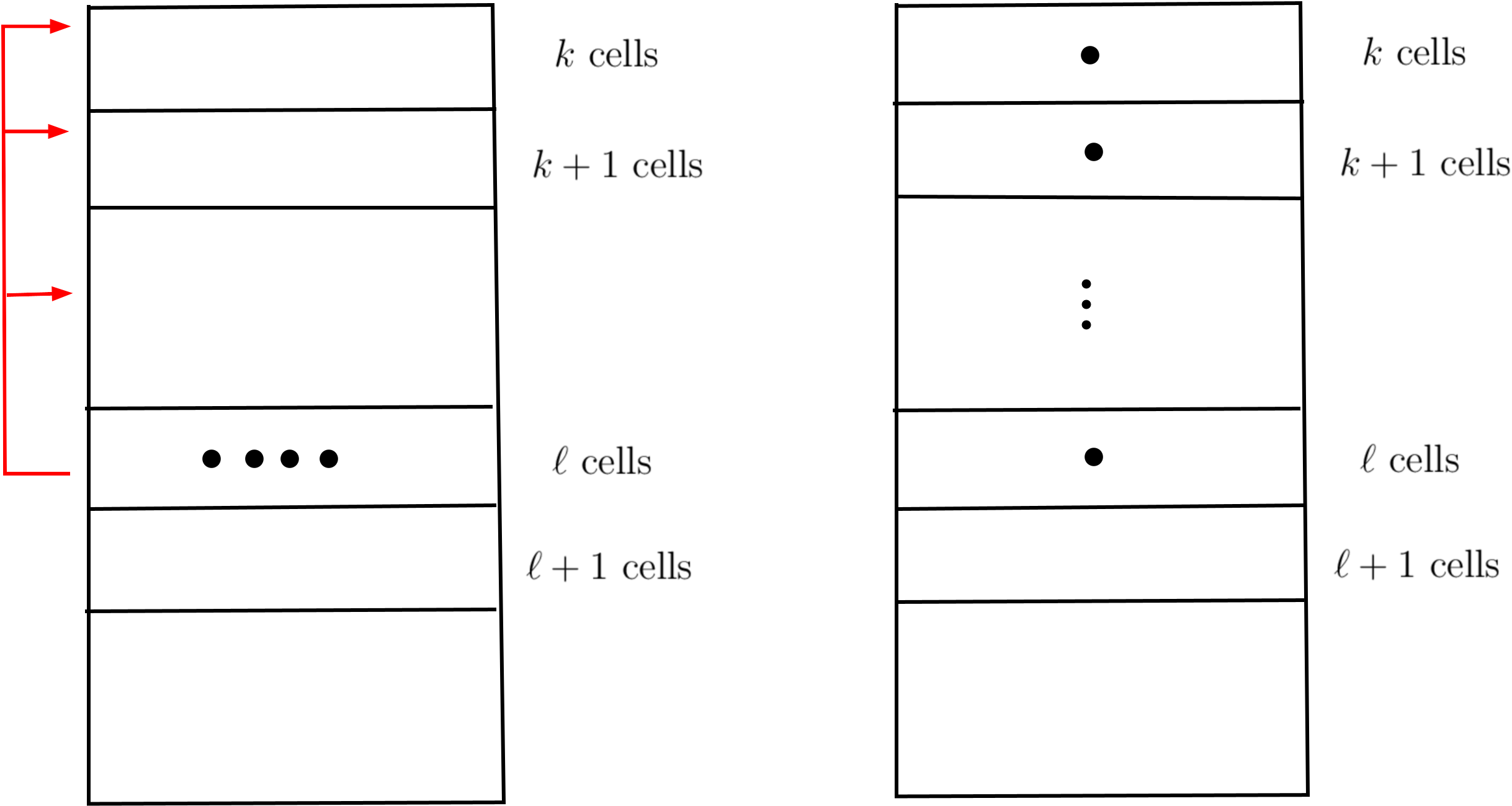
Figure 12. An illustration for moving the degrees of freedom in the high order case. Specifically, for each $\ell$-face $F$, we move all of its degrees of freedom to the lower - dimensional faces. In this case, $m$-faces with $m$ ranging from $k$ to $\ell$ can receive the degrees of freedom. If we take a closer look at the basis function of $\mathcal{P}_{r}^{-}\mathrm{Alt}^{k}(F)$ (where $\mathcal{P}_{r}^{-}\mathrm{Alt}^{k}(F)$ represents a certain function space related to our finite element construction), we can find that the possible dimensions $m$ of the faces that receive the degrees of freedom are in the range $m\in[k,\min(k+r,\ell)]$. Note that when $k+r\geq\ell$, some degrees of freedom will in fact stay in the face $F$.

Proof of Theorem 6.1, (3).

Similar to the previous proof, we still move the degrees of freedom to obtain the desired construction, see Figure 13. We first assume that $k<\ell$, where the degrees of freedom of the finite element space $C_{\iota^{*}\iota^{*}}\mathcal{P}^{-}\mathrm{Alt}^{k,\ell}$ are located on the simplices of dimensions greater than or equal to $\ell$, $\mathcal{T}_{\ell},\mathcal{T}_{\ell+1},\cdots.$ To impose the $\iota^{*}\jmath_{[p]}^{*}$-conformity, we move the degrees of freedom on simplices of dimension $\ell,\ell+1,\cdots,\ell+p-1$ to $m$-simplices $\sigma$ for $m\in[k,\ell+p-1]$.

Now we fix $\sigma$. The new degrees of freedom on $\sigma$ gained from those on $\mathcal{T}_{\ell+s}$ will ensure that the generalized trace $\iota^{\ast}\vartheta_{\sigma,k-s}^{*}$ is single-valued on $\sigma$. Therefore, we move the degrees of freedom and obtain the result. ∎

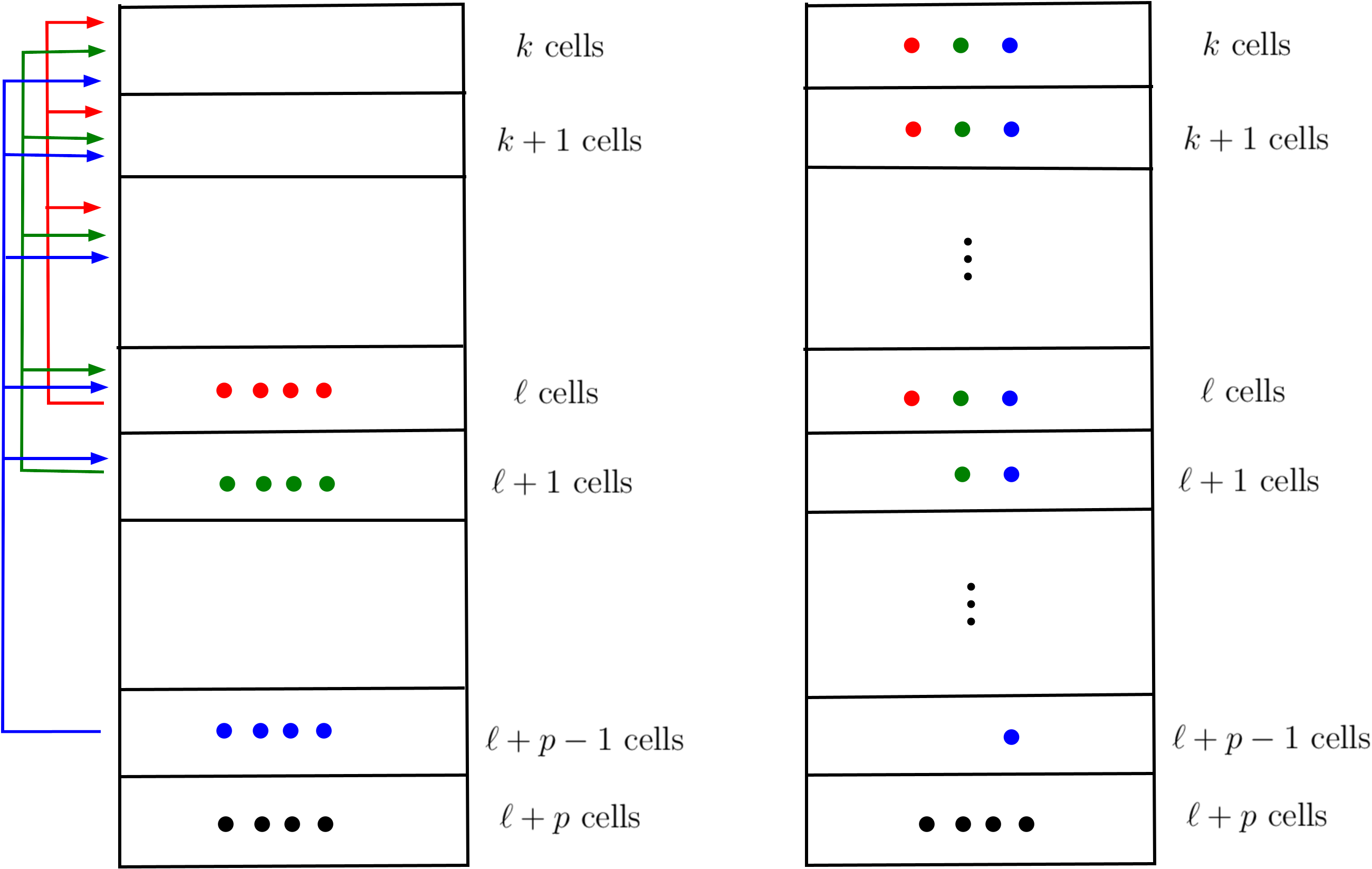
Figure 13. An illustration for moving the degrees of freedom in the high order case for $\iota^{*}\jmath_{[p]}^{*}$-conformity. For each $\ell+s$ with $s=0,1,\cdots,p-1$, we transfer the degrees of freedom to lower-dimensional faces. Note that it is possible that $k>\ell$. When this situation occurs, the $\iota^{*}\iota^{*}$-conforming construction will indicate that there are no degrees of freedom for $\ell,\ell+1,\cdots,k-1$ faces. Thus, the procedure of moving the degrees of freedom will start from $k$ faces.

Lemma 6.2.

If $k\leq\ell+p-1$, then $\mathcal{S}_{\dagger,[p]}:\mathcal{B}_{r}^{-}\mathrm{Alt}^{k,\ell}(\sigma)\to\mathcal{B}_{r}^{-}\mathrm{Alt}^{k-p,\ell+p}(\sigma)$ is onto.

The proof is based on Corollary 6.2, and be shown in the appendix. Using this lemma, we can repeat the symmetric reduction procedure in Section 4.

Theorem 6.2.

Let

$$\mathcal{P}_{r}^{-}{\mathbb{W}}_{[p]}^{k,\ell}:\mathcal{N}(\mathcal{S}_{\dagger,[p]}^{k,\ell}:\mathcal{P}_{r}^{-}\mathrm{Alt}^{k,\ell}\to\mathcal{P}_{r}^{-}\mathrm{Alt}^{k-p,\ell+p}).$$

Define

$$\mathcal{B}_{r}^{-}\mathbb{W}^{k,\ell}_{[p]}(\sigma)=\mathcal{N}(\mathcal{S}^{k,\ell}_{[p]}:\mathcal{B}_{r}^{-}\mathrm{Alt}^{k,\ell}(\sigma)\to\mathcal{B}_{r}^{-}\mathrm{Alt}^{k-p,\ell+p}(\sigma)),$$

whose dimension is

$$\dim\mathcal{B}_{r}^{-}\mathbb{W}^{k,\ell}_{[p]}(\sigma)=\dim\mathcal{B}_{r}^{-}\mathrm{Alt}^{k,\ell}(\sigma)-\dim\mathcal{B}_{r}^{-}\mathrm{Alt}^{k-p,\ell+p}(\sigma)).$$

The following DoFs are unisolvent with respect to the shape function space $\mathcal{P}^{-}_{r}{\mathbb{W}}^{k,\ell}_{[p]}(K)$:

1. $$\begin{cases}\langle\iota^{*}_{\sigma}\jmath^{*}_{\sigma}\omega,b\rangle_{\sigma},&\forall~~b\in\mathcal{B}_{r}^{-}\mathrm{Alt}^{k}(\sigma)\otimes\mathrm{Alt}^{l-m}(\sigma^{\perp}),\quad\dim\sigma=m\in[k,\ell],\\ \langle\iota^{*}_{\sigma}\iota^{*}_{\sigma}\omega,b\rangle_{\sigma},&\forall~~b\in\mathcal{B}_{r}^{-}{\mathbb{W}}^{k,l}(\sigma),\quad\dim\sigma>l.\end{cases}$$

   The resulting finite element space is $\iota^{*}\jmath^{*}$-conforming.

2. $$\begin{cases}\langle\iota^{*}_{\sigma}\jmath^{*}_{\sigma,[p]}\omega,b\rangle_{\sigma},&\forall~~b\in\bigoplus_{s=0}^{p-1}\mathcal{B}_{r}^{-}\mathrm{Alt}^{k}(\sigma)\otimes(\mathrm{Alt}^{m-s}(\sigma)\otimes\mathrm{Alt}^{\ell-m+s}(\sigma^{\perp})),\\ &\quad\dim\sigma=m\in[k,\ell+p-1],\\ \langle\iota^{*}_{\sigma}\iota^{*}_{\sigma}\omega,b\rangle_{\sigma},&\forall~~b\in\mathcal{B}^{-}_{r}{\mathbb{W}}^{k,l}_{[p]}(\sigma),\quad\dim\sigma\geq\ell+p.\end{cases}$$

   The resulting finite element space is $\iota^{*}\jmath^{*}_{[p]}$-conforming.

Using Theorem 6.1, we can finish the proof.

6.2. $\mathcal{P}_{r}\mathrm{Alt}^{k,\ell}$ family

We have

$$\dim\mathcal{P}_{r}\mathrm{Alt}^{k,\ell}=\binom{n+r}{n}\binom{n}{k}\binom{n}{\ell}.$$

We introduce

(6.11) $$\mathcal{B}_{r}\mathrm{Alt}^{k,\ell}(K):=\{\omega\in\mathcal{P}_{r}\mathrm{Alt}^{k,\ell}(\sigma):\iota_{F}^{**}K=0\,\,\forall F\triangleleft K,F\neq K\}.$$

Similar to Lemma 6.1 and Lemma 4.1, the following lemma holds.

Lemma 6.3.

Let $\psi_{\sigma,i}$ be a basis of $C_{\iota^{*}}\mathcal{P}_{r}\mathrm{Alt}^{k}$, with respect to the degrees of freedom on $\sigma$. Then it holds that,

$$\mathcal{B}_{r}\mathrm{Alt}^{k,\ell}(K)=\sum_{m=k}^{n}\sum_{\sigma\in\mathcal{T}_{\geq k}(K)}[\operatorname{span}_{i}\psi_{\sigma,i}]\otimes N^{\ell}(\sigma,K).$$

Therefore, the dimension of the bubble in $n$ dimension is

(6.12) $$\begin{split}\dim\mathcal{B}_{r}\mathrm{Alt}^{k,\ell}(K)=\sum_{m=k}^{n}\binom{n+1}{m+1}\Big{[}\binom{r+k}{r}\binom{r-1}{m-k}\Big{]}\cdot\binom{m}{\ell+m-n},\end{split}$$

since

$$\dim\mathcal{P}^{-}_{r+k-m}\mathrm{Alt}^{m-k}(\mathbb{R}^{m})=\binom{r+k}{r}\binom{r-1}{m-k}.$$

Corollary 6.3.

$\dim\mathcal{B}_{r}\mathrm{Alt}^{k,\ell}(K)=0$ if $\dim K\geq\ell+k+r$,

Corollary 6.4.

The set

$$\lambda^{\alpha}d\lambda_{I}\otimes d\lambda_{J}:|\alpha|=r,\operatorname{supp}\alpha\cup I\cup J=[n+1],$$

is a spanning set of $\mathcal{B}_{r}\mathrm{Alt}^{k,\ell}(K).$

Lemma 6.4.

If $k\leq\ell+p$, then $\mathcal{S}_{\dagger,[p]}:\mathcal{B}_{r}\mathrm{Alt}^{k,\ell}(\sigma)\to\mathcal{B}_{r}\mathrm{Alt}^{k-p,\ell+p}(\sigma)$ is onto.

The proof is based on Corollary 6.4, and be shown in the appendix.

Theorem 6.3.

The following DoFs are unisolvent with respect to the shape function space $\mathcal{P}^{r}\mathrm{Alt}^{k,\ell}(K)$:

1. (6.13) $$\langle\iota^{*}_{\sigma}\iota^{*}_{\sigma}\omega,b\rangle_{\sigma},\qquad\forall~~b\in\mathcal{B}_{r}\mathrm{Alt}^{k,l}(\sigma),\quad\forall\sigma\in\mathcal{T}(K).$$

   The resulting finite element space is $\iota^{*}\iota^{*}$-conforming.

2. $$\begin{cases}\langle\iota^{*}_{\sigma}\jmath^{*}_{\sigma}\omega,b\rangle_{\sigma},&\forall~~b\in\mathcal{B}_{r}\mathrm{Alt}^{k}(\sigma)\otimes\mathrm{Alt}^{l-m}(\sigma^{\perp}),\quad\dim\sigma=m\in[k,\ell],\\ \langle\iota^{*}_{\sigma}\iota^{*}_{\sigma}\omega,b\rangle_{\sigma},&\forall~~b\in\mathcal{B}_{r}\mathrm{Alt}^{k,l}(\sigma),\quad\dim\sigma>l.\end{cases}$$

   The resulting finite element space is $\iota^{*}\jmath^{*}$-conforming.

3. $$\begin{cases}\langle\iota^{*}_{\sigma}\jmath^{*}_{\sigma,[p]}\omega,b\rangle_{\sigma},&\forall~~b\in\bigoplus_{s=0}^{p-1}\mathcal{B}_{r}\mathrm{Alt}^{k}(\sigma)\otimes(\mathrm{Alt}^{m-s}(\sigma)\otimes\mathrm{Alt}^{\ell-m+s}(\sigma^{\perp})),\\ &\quad\dim\sigma=m\in[k,\ell+p-1],\\ \langle\iota^{*}_{\sigma}\iota^{*}_{\sigma}\omega,b\rangle_{\sigma},&\forall~~b\in\mathcal{B}_{r}\mathrm{Alt}^{k,\ell}(\sigma),\quad\dim\sigma\geq\ell+p.\end{cases}$$

   The resulting finite element space is $\iota^{*}\jmath^{*}_{[p]}$-conforming.

Proof.

It suffices to show the dimension counting in (1), and the remaining proofs are similar. The dimension counting reads

(6.14) $$\begin{split}\sum_{\sigma\in\mathcal{T}(K)}\dim\mathcal{B}_{r}\mathrm{Alt}^{k,\ell}(\sigma)=&\sum_{n^{\prime}}\binom{n+1}{n^{\prime}+1}\sum_{m=k}^{n}\binom{n^{\prime}+1}{m+1}\Big{[}\binom{r+k}{r}\binom{r-1}{m-k}\Big{]}\cdot\binom{m}{\ell+m-n^{\prime}}\\ =&\sum_{m}\Big{[}\binom{r+k}{r}\binom{r-1}{m-k}\Big{]}\sum_{n^{\prime}}\binom{n+1}{n^{\prime}+1}\binom{n^{\prime}+1}{m+1}\cdot\binom{m}{\ell+m-n^{\prime}}\\ =&\sum_{m}\binom{r+k}{r}\binom{r-1}{m-k}\binom{n+1}{m+1}\binom{n}{n-\ell}\\ =&\binom{r+k}{r}\binom{r+n}{r+k}\binom{n}{\ell}.\end{split}$$

Here, we use the fact $\displaystyle\binom{r-1}{m-k}=\binom{r-1}{r-1-m+k}$ and the Vandermonde identity. ∎

Thus, we can do the symmetry reduction, leading to the following theorem.

Theorem 6.4.

Let

$$\mathcal{P}_{r}{\mathbb{W}}_{[p]}^{k,\ell}:\mathcal{N}(\mathcal{S}_{\dagger,[p]}^{k,\ell}:\mathcal{P}_{r}\mathrm{Alt}^{k,\ell}\to\mathcal{P}_{r}\mathrm{Alt}^{k-p,\ell+p}).$$

Define

$$\mathcal{B}_{r}\mathbb{W}^{k,\ell}_{[p]}(\sigma)=\mathcal{N}(\mathcal{S}^{k,\ell}_{[p]}:\mathcal{B}_{r}\mathrm{Alt}^{k,\ell}(\sigma)\to\mathcal{B}_{r}\mathrm{Alt}^{k-p,\ell+p}(\sigma)),$$

whose dimension is

$$\dim\mathcal{B}_{r}\mathbb{W}^{k,\ell}_{[p]}(\sigma)=\dim\mathcal{B}_{r}\mathrm{Alt}^{k,\ell}(\sigma)-\dim\mathcal{B}_{r}\mathrm{Alt}^{k-p,\ell+p}(\sigma)).$$

The following DoFs are unisolvent with respect to the shape function space $\mathcal{P}^{-}_{r}{\mathbb{W}}^{k,\ell}_{[p]}(K)$:

1. $$\begin{cases}\langle\iota^{*}_{\sigma}\jmath^{*}_{\sigma}\omega,b\rangle_{\sigma},&\forall~~b\in\mathcal{B}_{r}\mathrm{Alt}^{k}(\sigma)\otimes\mathrm{Alt}^{\ell-m}(\sigma^{\perp}),\quad\dim\sigma=m\in[k,\ell],\\ \langle\iota^{*}_{\sigma}\iota^{*}_{\sigma}\omega,b\rangle_{\sigma},&\forall~~b\in\mathcal{B}_{r}{\mathbb{W}}^{k,\ell}(\sigma),\quad\dim\sigma>\ell.\end{cases}$$

   The resulting finite element space is $\iota^{*}\jmath^{*}$-conforming.

2. $$\begin{cases}\langle\iota^{*}_{\sigma}\jmath^{*}_{\sigma,[p]}\omega,b\rangle_{\sigma},&\forall~~b\in\bigoplus_{s=0}^{p-1}\mathcal{B}_{r}\mathrm{Alt}^{k}(\sigma)\otimes(\mathrm{Alt}^{m-s}(\sigma)\otimes\mathrm{Alt}^{\ell-m+s}(\sigma^{\perp})),\\ &\quad\dim\sigma=m\in[k,\ell+p-1],\\ \langle\iota^{*}_{\sigma}\iota^{*}_{\sigma}\omega,b\rangle_{\sigma},&\forall~~b\in\mathcal{B}_{r}{\mathbb{W}}^{k,\ell}_{[p]}(\sigma),\quad\dim\sigma\geq\ell+p.\end{cases}$$

   The resulting finite element space is $\iota^{*}\jmath^{*}_{[p]}$-conforming.

6.3. High order Regge elements

To close this subsection, we prove that when $k=\ell=1,p=1$, the above construction recovers the higher order Regge element in any dimension, cf. [44].

For $\mathcal{P}_{r}\mathrm{Alt}^{1,1}$ form, the numbers of degrees of freedom on simplex $K$ are

(6.15) $$\footnotesize\begin{split}\dim\mathcal{B}_{r}\mathrm{Alt}^{1,1}(K)=&\sum_{m=k}^{n}\binom{n+1}{m+1}\Big{[}\binom{r+1}{r}\binom{r-1}{m-1}\Big{]}\cdot\binom{m}{n-1}\\ =&\binom{n+1}{n}\binom{r+1}{r}\binom{r-1}{n-2}\binom{n-1}{n-1}+\binom{n+1}{n+1}\binom{r+1}{r}\binom{r-1}{n-1}\binom{n}{n-1}\\ =&(n+1)(r+1)\binom{r-1}{n-2}+n(r+1)\binom{r-1}{n-1}\\ =&n(r+1)\binom{r}{n-1}+(r+1)\binom{r-1}{n-2}\\ =&n^{2}\binom{r+1}{n}+(r+1)\binom{r-1}{n-2}\end{split}$$

For $\mathcal{P}_{r}\mathrm{Alt}^{0,2}$, the numbers of the degrees of freedom on simplex $K$ are

(6.16) $$\footnotesize\begin{split}\dim\mathcal{B}_{r}\mathrm{Alt}^{0,2}(K)=&\sum_{m=k}^{n}\binom{n+1}{m+1}\Big{[}\binom{r}{r}\binom{r-1}{m}\Big{]}\cdot\binom{m}{n-2},\\ =&\binom{n+1}{n-1}\binom{r-1}{n-2}\binom{n-2}{n-2}+\binom{n+1}{n}\binom{r-1}{n-1}\binom{n-1}{n-2}+\binom{n+1}{n+1}\binom{r-1}{n}\binom{n}{n-2}\\ =&\binom{n+1}{2}\binom{r-1}{n-2}+(n^{2}-1)\binom{r-1}{n-1}+\binom{n}{2}\binom{r-1}{n}\\ =&\binom{n+1}{2}\binom{r}{n-1}+\binom{n}{2}\binom{r}{n}-\binom{r-1}{n-1}.\end{split}$$

For $\mathcal{P}_{r}\mathbb{W}^{1,1}$ form, the numbers of degrees of freedom on simplex $K$ are

(6.17) $$\begin{split}&\dim\mathcal{B}_{r}\mathrm{Alt}^{1,1}(K)-\dim\mathcal{B}_{r}\mathrm{Alt}^{0,2}(K)\\ =&n^{2}\binom{r+1}{n}+(r+1)\binom{r-1}{n-2}-\binom{n+1}{2}\binom{r}{n-1}-\binom{n}{2}\binom{r}{n}+\binom{r-1}{n-1}\\ =&\binom{n}{2}\binom{r}{n-1}+\binom{n+1}{2}\binom{r}{n}+\binom{r}{n-1}+r\binom{r-1}{n-2}\\ =&\binom{n}{2}\binom{r}{n-1}+\binom{n+1}{2}\binom{r}{n}+\binom{r}{n-1}+(n-1)\binom{r}{n-1}\\ =&\binom{n}{2}\binom{r}{n-1}+\binom{n+1}{2}\binom{r}{n}+n\binom{r}{n-1}\\ =&\binom{n+1}{2}\binom{r+1}{n}\end{split}$$

which is equal to $\dim\mathcal{P}_{r-n+1}\mathbb{W}^{1,1}$, the dimension of degrees of freedom of Regge elements in [44]. It is not difficult to check the two finite elements give the same space.

7. Higher order examples in 3D

7.1. $\mathcal{P}_{r}\mathbb{W}^{1,1}$ element

For $\mathcal{P}_{r}\mathbb{W}^{1,1}$ family, the shape function is $\mathcal{P}_{r}\otimes\mathbb{S}$, whose dimension is $(r+3)(r+2)(r+1)$. The degrees of freedom are

$$\int_{e}\bm{\sigma}_{tt}\cdot q,\quad\forall q\in\mathcal{P}_{r}(e) \text{count}=(r+1)$$

$$\int_{f}\bm{\sigma}_{tt}\cdot q,\quad\forall q\in\mathcal{B}_{r}\mathbb{W}^{1,1}(f) \text{count}=\frac{3}{2}(r+1)(r)$$

$$\int_{K}\bm{\sigma}\cdot q,\quad\forall q\in\mathcal{B}_{r}\mathbb{W}^{1,1}(K) \text{count}=(r+1)r(r-1)$$

7.2. $\mathcal{P}_{r}^{-}\mathbb{W}^{1,1}$ element

We illustrate it in two dimensions in this subsection, and three dimensions in the next subsection.

In two dimensions, the shape function space is the kernel of

(7.1) $$\begin{split}\mathcal{N}(\operatorname{skw}:\mathcal{P}_{r-1}\mathbb{M}^{2}+\bm{x}\otimes\mathcal{P}_{r-1}\mathbb{V}^{2}\to\mathcal{P}_{r})=&\mathcal{P}_{r-1}\mathbb{S}^{2}+\bm{x}^{\perp}\otimes\bm{x}^{\perp}\mathcal{P}_{r-2}\end{split}$$

The dimension is

$$\dim\mathcal{P}_{r}^{-}\mathrm{Alt}^{1,1}-\dim\mathcal{P}_{r}^{-}\mathrm{Alt}^{0,2}=2(r^{2}+2r)-\binom{r+2}{2}=\frac{1}{2}(r+2)(3r-1),$$

and the degrees of freedom are

$$\int_{e}\bm{\sigma}_{tt}\cdot q,\quad\forall q\in\mathcal{P}_{r-1}(e) \text{count}=r$$

$$\int_{f}\bm{\sigma}_{tt}\cdot q,\quad\forall q\in\mathcal{B}_{r}^{-}\mathbb{W}^{1,1}(f) \text{count}=\frac{1}{2}(3r+2)(r-1)$$

Here

(7.2) $$\begin{split}\mathcal{B}_{r}^{-}\mathbb{W}^{1,1}(f)=&\dim\mathcal{B}_{r}^{-}\mathrm{Alt}^{1,1}(f)-\dim\mathcal{B}_{r}^{-}\mathrm{Alt}^{0,2}(f)\\ =&r(2r+1)-\frac{1}{2}(r+2)(r+1)=\frac{1}{2}(3r+2)(r-1).\end{split}$$

Now we consider the three dimensional cases. For $\mathcal{P}_{r}^{-}\mathbb{W}^{1,1}$, the shape function space is

(7.3) $$\begin{split}\mathcal{N}(\operatorname{skw}:\mathcal{P}_{r-1}\mathbb{M}+\bm{x}\times\mathcal{P}_{r-1}\mathbb{M}\to\mathcal{P}_{r}\mathbb{V})=&\mathcal{P}_{r-1}\mathbb{S}+\bm{x}\times\mathcal{P}_{r-2}\mathbb{S}\times\bm{x}\end{split}$$

whose dimension is

(7.4) $$\begin{split}\dim\mathcal{P}_{r}^{-}\mathrm{Alt}^{1,1}-\dim\mathcal{P}_{r}^{-}\mathrm{Alt}^{0,2}=&\frac{3}{2}r(r+2)(r+3)-\frac{1}{2}(r+1)(r+2)(r+3)\\ =&\frac{1}{2}(r+2)(r+3)(2r-1).\end{split}$$

The degrees of freedom are

$$\int_{e}\bm{\sigma}_{tt}\cdot q,\quad\forall q\in\mathcal{P}_{r-1}(e) \text{count}=r$$

$$\int_{f}\bm{\sigma}_{tt}\cdot q,\quad\forall q\in\mathcal{B}_{r}^{-}\mathbb{W}^{1,1}(f) \text{count}=\frac{1}{2}(3r+2)(r-1)$$

$$\int_{K}\bm{\sigma}\cdot q,\quad\forall q\in\mathcal{B}_{r}^{-}\mathbb{W}^{1,1}(K) \text{count}=\frac{1}{2}(r-1)(2r^{2}-r-2)$$

Here in three dimensions,

(7.5) $$\begin{split}\dim\mathcal{B}_{r}^{-}\mathrm{Alt}^{1,1}-\dim\mathcal{B}_{r}^{-}\mathrm{Alt}^{0,2}=&\frac{1}{2}(r-1)r(3r+2)-\frac{1}{2}(r-1)(r+1)(r+2)\\ =&\frac{1}{2}(r-1)(2r^{2}-r-2)\end{split}$$

7.3. $\mathcal{P}_{r}\mathbb{W}^{1,2}$ element

For $\mathcal{P}_{r}\mathbb{W}^{1,2}$ family, the shape function space is $\mathcal{P}_{r}\otimes\mathbb{T}$, whose dimension is $\frac{4}{3}(r+3)(r+2)(r+1)$.

The degrees of freedom are

$$\int_{e}\bm{\sigma}_{tn}\cdot q,\quad\forall q\in\mathcal{P}_{r}(e)\otimes\mathbb{R}^{2} \text{count}=2(r+1)$$

$$\int_{f}\bm{\sigma}_{tn}\cdot q,\quad\forall q\in\mathcal{B}_{r}\mathrm{Alt}^{1}(f)\otimes\mathrm{Alt}^{0}(f) \text{count}=(r^{2}-1)$$

$$\int_{K}\bm{\sigma}\cdot q,\quad\forall q\in\mathcal{B}_{r}\mathbb{W}^{1,2}(K) \text{count}=\frac{3}{4}(r+1)(r+2)r$$

Here,

(7.6) $$\begin{split}\dim\mathcal{B}_{r}\mathrm{Alt}^{1,2}-\dim\mathcal{B}_{r}\mathrm{Alt}^{0,3}=&\frac{1}{2}(r+1)(r+2)(3r+1)-\frac{1}{6}(r+1)(r+2)(r+3)\\ =&\frac{3}{4}(r+1)(r+2)r\end{split}$$

7.4. $\mathcal{P}_{r}^{-}\mathbb{W}^{1,2}$ element

For $\mathcal{P}_{r}^{-}\mathbb{W}^{1,2}$ family, the shape function space is

(7.7) $$\begin{split}\mathcal{N}(\operatorname{tr}:\mathcal{P}_{r-1}\mathbb{M}+\bm{x}\times\mathcal{P}_{r-1}\mathbb{M}\to\mathcal{P}_{r}\mathbb{V})=&\mathcal{P}_{r}\mathbb{T}+\bm{x}\times(\mathcal{P}_{r-1}\mathbb{S})+\bm{x}\times(\mathcal{P}_{r-2}\mathbb{V}\bm{x})\end{split}$$

whose dimension is

(7.8) $$\begin{split}\dim\mathcal{P}_{r}^{-}\mathrm{Alt}^{1,2}-\dim\mathcal{P}_{r}^{-}\mathrm{Alt}^{0,3}=&\frac{3}{2}r(r+2)(r+3)-\frac{1}{6}(r+1)(r+2)(r+3)\\ =&\frac{1}{6}(r+2)(r+3)(8r-1).\end{split}$$

The degrees of freedom are

$$\int_{e}\bm{\sigma}_{tn}\cdot q,\quad\forall q\in\mathcal{P}_{r-1}(e)\otimes\mathbb{R}^{2} \text{count}=2r$$

$$\int_{f}\bm{\sigma}_{tn}\cdot q,\quad\forall q\in\mathcal{B}_{r}^{-}\mathrm{Alt}^{1}(f)\otimes\mathrm{Alt}^{0}(f) \text{count}=r(r-1)$$

$$\int_{K}\bm{\sigma}\cdot q,\quad\forall q\in\mathcal{B}_{r}^{-}\mathbb{W}^{1,2}(K) \text{count}=\frac{1}{6}(r+2)(8r^{2}-r-3)$$

Here

(7.9) $$\begin{split}\dim\mathcal{B}_{r}^{-}\mathrm{Alt}^{1,2}-\dim\mathcal{B}_{r}^{-}\mathrm{Alt}^{0,3}=&\frac{1}{2}r(r+2)(3r+1)-\frac{1}{6}(r+1)(r+2)(r+3)\\ =&\frac{1}{6}(r+2)(8r^{2}-r-3)\end{split}$$

7.5. $\mathcal{P}_{r}\mathbb{W}^{2,2}$ element

For $\mathcal{P}_{r}\mathbb{W}^{2,2}$ family, the shape function space is $\mathcal{P}_{r}\otimes\mathbb{S}$, whose dimension is $(r+3)(r+2)(r+1)$. The degrees of freedom are

$$\int_{f}\bm{\sigma}_{nn}\cdot q,\quad\forall q\in\mathcal{P}_{r}(f) \text{count}=\frac{1}{2}(r+2)(r+1)$$

$$\int_{K}\bm{\sigma}\cdot q,\quad\forall q\in\mathcal{B}_{r}\mathbb{W}^{2,2}(K) \text{count}=(r+1)^{2}(r+2)$$

Here

(7.10) $$\footnotesize\begin{split}\dim\mathcal{B}_{r}\mathrm{Alt}^{2,2}-\dim\mathcal{B}_{r}\mathrm{Alt}^{1,3}=&\frac{1}{2}(r+1)(r+2)(3r+5)-\frac{1}{2}(r+1)(r+2)(r+3)\\ =&(r+1)^{2}(r+2)\end{split}$$

7.6. $\mathcal{P}_{r}^{-}\mathbb{W}^{2,2}$ element

For $\mathcal{P}_{r}^{-}\mathbb{W}^{2,2}$ family, the shape function space is

(7.11) $$\begin{split}\mathcal{N}(\operatorname{skw}:\mathcal{P}_{r-1}(\mathbb{M})+\bm{x}\mathcal{P}_{r-1}\mathbb{V}\to\mathcal{P}_{r-1}\mathbb{V}+\bm{x}\times P_{r-1}\mathbb{V})=&\mathcal{P}_{r-1}\mathbb{S}+\bm{x}\otimes\bm{x}\mathcal{P}_{r-2}\end{split}$$

whose dimension is

(7.12) $$\begin{split}\dim\mathcal{P}_{r}^{-}\mathrm{Alt}^{2,2}-\dim\mathcal{P}_{r}^{-}\mathrm{Alt}^{1,3}=&\frac{3}{2}r(r+1)(r+3)-\frac{1}{2}r(r+2)(r+3)\\ =&\frac{1}{2}r(r+3)(2r+1).\end{split}$$

the degrees of freedom are

$$\int_{f}\bm{\sigma}_{nn}\cdot q,\quad\forall q\in\mathcal{P}_{r-1}(f) \text{count}=\frac{1}{2}(r+1)r$$

$$\int_{K}\bm{\sigma}\cdot q,\quad\forall q\in\mathcal{B}_{r}^{-}\mathbb{W}^{2,2}(K) \text{count}=\frac{1}{2}r(2r^{2}+3r-1)$$

Here

(7.13) $$\begin{split}\dim\mathcal{B}_{r}^{-}\mathrm{Alt}^{2,2}-\dim\mathcal{B}_{r}^{-}\mathrm{Alt}^{1,3}=&\frac{1}{2}r(r+1)(3r+5)-\frac{1}{2}r(r+2)(r+3)\\ =&\frac{1}{2}r(2r^{2}+3r-1)\end{split}$$

7.7. $\mathcal{P}_{r}\mathbb{W}_{[2]}^{2,1}$ element

For $\mathcal{P}_{r}\mathbb{W}^{2,1}_{[2]}$ family, the shape function space is $\mathcal{P}_{r}\otimes\mathbb{T}$, whose dimension is $\frac{4}{3}(r+3)(r+2)(r+1)$. the degrees of freedom are

$$\int_{f}\bm{\sigma}_{nt}\cdot q,\quad\forall q\in\mathcal{P}_{r}(f)\otimes\mathbb{R}^{2} \text{count}=(r+2)(r+1)$$

$$\int_{K}\bm{\sigma}\cdot q,\quad\forall q\in\mathcal{B}_{r}\mathbb{W}^{2,1}(K) \text{count}=\frac{4}{3}(r+1)(r+2)r$$

Here,

(7.14) $$\begin{split}\dim\mathcal{B}_{r}\mathrm{Alt}^{2,1}-\dim\mathcal{B}_{r}\mathrm{Alt}^{0,3}=&\frac{1}{2}(r+1)(r+2)(3r+1)-\frac{1}{6}(r+1)(r+2)(r+3)\\ =&\frac{4}{3}(r+1)(r+2)r.\end{split}$$

7.8. $\mathcal{P}_{r}^{-}\mathbb{W}_{[2]}^{2,1}$ element

For $\mathcal{P}_{r}^{-}\mathbb{W}^{2,1}$ family, the shape function space is

(7.15) $$\begin{split}\mathcal{N}(\operatorname{tr}:\mathcal{P}_{r-1}\mathbb{M}+\bm{x}\mathcal{P}_{r-1}\mathbb{V}\to\mathcal{P}_{r-1}\mathbb{V}+\bm{x}\cdot P_{r-1}\mathbb{V})=&\mathcal{P}_{r-1}\mathbb{T}+\bm{x}\times\mathcal{P}_{r-2}\bm{x}\end{split}$$

whose dimension is

(7.16) $$\begin{split}\dim\mathcal{P}_{r}^{-}\mathrm{Alt}^{2,1}-\dim\mathcal{P}_{r}^{-}\mathrm{Alt}^{0,3}=&\frac{3}{2}r(r+1)(r+3)-\frac{1}{6}(r+1)(r+2)(r+3)\\ =&\frac{1}{3}(4r-1)(r+1)(r+3).\end{split}$$

The degrees of freedom are

$$\int_{f}\bm{\sigma}_{nt}\cdot q,\quad\forall q\in\mathcal{P}_{r-1}(f)\otimes\mathbb{R}^{2} \text{count}=(r+1)r$$

$$\int_{K}\bm{\sigma}\cdot q,\quad\forall q\in\mathcal{B}_{r}^{-}\mathbb{W}^{2,1}(K) \text{count}=\frac{1}{3}(r+1)(4r+3)(r-1)$$

Here

(7.17) $$\begin{split}\dim\mathcal{B}_{r}^{-}\mathrm{Alt}^{2,1}-\dim\mathcal{B}_{r}^{-}\mathrm{Alt}^{0,3}=&\frac{1}{2}r(3r^{2}+4r+1)-\frac{1}{6}(r+1)(r+2)(r+3)\\ =&\frac{1}{3}(r+1)(4r+3)(r-1).\end{split}$$

Appendix A Technical Details on BGG Framework

We first show the proof of Lemma 2.1, (1).

Lemma A.1.

$\operatorname{\mathcal{S}}$ and $\operatorname{\mathcal{S}}_{\dagger}$ are adjoint with respect to the standard Frobenius norm, i.e.,

$$(\mathcal{S}^{k,\ell}\omega,\mu)=(\omega,\mathcal{S}^{k+1,\ell-1}_{\dagger}\mu),\quad\forall\omega\in\mathrm{Alt}^{k,\ell},\mu\in\mathrm{Alt}^{k+1,\ell-1}.$$

Proof.

Let $\omega:=dx^{\sigma_{1}}\wedge\cdots\wedge dx^{\sigma_{k}}\otimes dx^{\tau_{1}}\wedge\cdots\wedge dx^{\tau_{\ell}}$ (as a default convention of notation, we assume that $\sigma_{1},\cdots,\sigma_{k}$ are different from each other, and similar for $\tau_{1},\cdots,\tau_{\ell}$; otherwise $\omega=0$ and the theorem is trivial). Then

$$\mathcal{S}^{k,\ell}\omega=\sum_{j=1}^{\ell}(-1)^{\ell+1}dx^{\tau_{j}}\wedge dx^{\sigma_{1}}\wedge\cdots\wedge dx^{\sigma_{k}}\otimes dx^{\tau_{1}}\wedge\cdots\wedge\widehat{dx^{\tau_{j}}}\wedge\cdots\wedge dx^{\tau_{\ell}}.$$

Let $\mu:=dx^{\alpha_{1}}\wedge\cdots\wedge dx^{\alpha_{k+1}}\otimes dx^{\beta_{1}}\wedge\cdots\wedge dx^{\beta_{\ell-1}}$. Consider the Frobenius inner product $(\mathcal{S}^{k,\ell}\omega,\mu)$. The inner product is nonzero only if

(A.1) $$\{\sigma_{1},\cdots,\sigma_{k}\}\subset\{\alpha_{1},\cdots,\alpha_{k+1}\},$$

and

(A.2) $$\{\beta_{1},\cdots,\beta_{\ell-1}\}\subset\{\tau_{1},\cdots,\tau_{\ell}\}.$$

Similarly,

$$\mathcal{S}^{k+1,\ell-1}_{\dagger}\mu=\sum_{j=1}^{k}(-1)^{k+1}dx^{\alpha_{1}}\wedge\cdots\wedge\widehat{dx^{\alpha_{j}}}\wedge\cdots\wedge dx^{\alpha_{k+1}}\otimes dx^{\alpha_{j}}\wedge dx^{\beta_{1}}\wedge\cdots\wedge dx^{\beta_{\ell-1}}.$$

We verify that if either (A.1) or (A.2) fails, then $(\mathcal{S}^{k,\ell}\omega,\mu)=0=(\omega,\mathcal{S}^{k+1,\ell-1}_{\dagger}\mu)$, which satisfies the theorem. Therefore hereafter we assume (A.1) and (A.2). Without loss of generality, we further assume (with the order)

$$\sigma_{1},\cdots,\sigma_{k}=\alpha_{2},\cdots,\alpha_{k+1},$$

and

$$\beta_{1},\cdots,\beta_{\ell-1}=\tau_{2},\cdots,\tau_{\ell}.$$

Then

$$(\mathcal{S}^{k,\ell}\omega,\mu)=-\delta^{\tau_{1},\alpha_{1}}=(\omega,\mathcal{S}^{k+1,\ell-1}_{\dagger}\mu).$$

The desired result follows as any element in $\mathrm{Alt}^{k,\ell}$ (or $\mathrm{Alt}^{k+1,\ell-1}$) can be written as a linear combination of monomials of the form of $\omega$ (or $\mu$) above. ∎

Lemma A.2.

The identity (2.11) holds. That is, $\kappa$ and $\mathcal{S}_{\dagger}$ commute.

Proof.

We give a direct proof. Let $\omega=dx^{\sigma_{1}}\wedge\cdots\wedge dx^{\sigma_{k}}\otimes dx^{\tau_{1}}\wedge\cdots\wedge dx^{\tau_{\ell}}$. Then

$$\kappa\omega=\sum_{i=1}^{k}(-1)^{i+1}x^{\sigma_{i}}dx^{\sigma_{1}}\wedge\cdots\wedge\widehat{dx^{\sigma_{i}}}\wedge\cdots\wedge dx^{\sigma_{k}}\otimes dx^{\sigma_{i}}\wedge dx^{\tau_{1}}\wedge\cdots\wedge dx^{\tau_{\ell}}.$$

$$\mathcal{S}_{\dagger}\kappa\omega=$$

$$\sum_{i=1}^{k}(-1)^{i+1}(\sum_{j=1}^{i-1}(-1)^{j+1}x^{\sigma_{i}}dx^{\sigma_{1}}\wedge\cdots\wedge\widehat{dx^{\sigma_{j}}}\wedge\cdots\wedge\widehat{dx^{\sigma_{i}}}\wedge\cdots\wedge dx^{\sigma_{k}}\otimes dx^{\sigma_{j}}\wedge dx^{\tau_{1}}\wedge\cdots\wedge dx^{\tau_{\ell}}$$

$$+\sum_{j=i+1}^{k}(-1)^{j}x^{\sigma_{i}}dx^{\sigma_{1}}\wedge\cdots\wedge\widehat{dx^{\sigma_{i}}}\wedge\cdots\wedge\widehat{dx^{\sigma_{j}}}\wedge\cdots\wedge dx^{\sigma_{k}}\otimes dx^{\sigma_{j}}\wedge dx^{\tau_{1}}\wedge\cdots\wedge dx^{\tau_{\ell}})$$

$$=\sum_{i=1}^{k}\sum_{j=1}^{i-1}(-1)^{i+j}x^{\sigma_{i}}dx^{\sigma_{1}}\wedge\cdots\wedge\widehat{dx^{\sigma_{j}}}\wedge\cdots\wedge\widehat{dx^{\sigma_{i}}}\wedge\cdots\wedge dx^{\sigma_{k}}\otimes dx^{\sigma_{j}}\wedge dx^{\tau_{1}}\wedge\cdots\wedge dx^{\tau_{\ell}}$$

$$+\sum_{i=1}^{k}\sum_{j=i+1}^{k}(-1)^{i+j+1}x^{\sigma_{i}}dx^{\sigma_{1}}\wedge\cdots\wedge\widehat{dx^{\sigma_{i}}}\wedge\cdots\wedge\widehat{dx^{\sigma_{j}}}\wedge\cdots\wedge dx^{\sigma_{k}}\otimes dx^{\sigma_{j}}\wedge dx^{\tau_{1}}\wedge\cdots\wedge dx^{\tau_{\ell}}.$$

Similarly,

$$\mathcal{S}_{\dagger}\omega=\sum_{j=1}^{k}(-1)^{j+1}dx^{\sigma_{1}}\wedge\cdots\wedge\widehat{dx^{\sigma_{j}}}\wedge\cdots\wedge dx^{\sigma_{k}}\otimes dx^{\sigma_{j}}\wedge dx^{\tau_{1}}\wedge\cdots\wedge dx^{\tau_{\ell}},$$

and

$$\kappa\mathcal{S}_{\dagger}\omega=$$

$$\sum_{j=1}^{k}(-1)^{j+1}(\sum_{i=1}^{j-1}(-1)^{i+1}x^{\sigma_{i}}dx^{\sigma_{1}}\wedge\cdots\wedge\widehat{dx^{\sigma_{i}}}\wedge\cdots\wedge\widehat{dx^{\sigma_{j}}}\wedge\cdots\wedge dx^{\sigma_{k}}\otimes dx^{\sigma_{j}}\wedge dx^{\tau_{1}}\wedge\cdots\wedge dx^{\tau_{\ell}}$$

$$+\sum_{i=j+1}^{k}(-1)^{i}x^{\sigma_{i}}dx^{\sigma_{1}}\wedge\cdots\wedge\widehat{dx^{\sigma_{j}}}\wedge\cdots\wedge\widehat{dx^{\sigma_{i}}}\wedge\cdots\wedge dx^{\sigma_{k}}\otimes dx^{\sigma_{j}}\wedge dx^{\tau_{1}}\wedge\cdots\wedge dx^{\tau_{\ell}})$$

$$=\sum_{i=1}^{k}\sum_{j=1}^{i-1}(-1)^{i+j}x^{\sigma_{i}}dx^{\sigma_{1}}\wedge\cdots\wedge\widehat{dx^{\sigma_{j}}}\wedge\cdots\wedge\widehat{dx^{\sigma_{i}}}\wedge\cdots\wedge dx^{\sigma_{k}}\otimes dx^{\sigma_{j}}\wedge dx^{\tau_{1}}\wedge\cdots\wedge dx^{\tau_{\ell}}$$

$$+\sum_{i=1}^{k}\sum_{j=i+1}^{k}(-1)^{i+j+1}x^{\sigma_{i}}dx^{\sigma_{1}}\wedge\cdots\wedge\widehat{dx^{\sigma_{i}}}\wedge\cdots\wedge\widehat{dx^{\sigma_{j}}}\wedge\cdots\wedge dx^{\sigma_{k}}\otimes dx^{\sigma_{j}}\wedge dx^{\tau_{1}}\wedge\cdots\wedge dx^{\tau_{\ell}},$$

where in the last step we swapped the dumb indices. ∎

Next, we show the injectivity, and the sujectivity result, as shown in Lemma 2.1, Lemma 2.4. For the bubble result, we will prove Lemma 4.3 and Lemma 4.4.

The proof we adopt here resembles to that in the appendix of [7]. However, we generalize the original proof to the iterated case and the bubble case.

Let $X(n,k)$ be the increase $k$-tuple in $[n]:=\{1,2,\cdots,n\}$. That is, $X(n,k):=\{\sigma\in[n]^{k}:\sigma_{1}<\sigma_{2}<\cdots<\sigma_{k}\}.$ Let $FX(n,k)$ be the free Abelian group generated by $X(n,k)$, and we use $[I]$ to represent the element associated with $I$. We then define $s:FX(n,k)\to FX(n,k+1)$ such that

$$s([I])=\sum_{j\in[n]\setminus I}[I\cup\{j\}],\quad\forall I\in X(n,k)$$

We also define $s_{\dagger}:FX(n,k+1)\to FX(n,k)$ such that

$$s_{\dagger}([J])=\sum_{j\in J}[J\setminus\{j\}],\quad\forall J\in X(n,k+1).$$

Lemma A.3.

1. When $n\geq 2k+1$, $s:FX(n,k)\to FX(n,k+1)$ is injective, $s_{\dagger}:FX(n,k+1)\to FX(n,k)$ is surjective.

2. When $n\leq 2k+1$, $s:FX(n,k)\to FX(n,k+1)$ is surjective, $s_{\dagger}:FX(n,k+1)\to FX(n,k)$ is injective.

Proof.

We introduce the inner product on $FX(n,k)$ such that $\langle[I],[J]\rangle=\delta_{IJ}.$ For $I,J\in X(n,k)$ it holds that

$$\langle s([I]),s([J])\rangle=\begin{cases}n-k&\mbox{ if }I=J\\ 1&\mbox{ if }\#I\cap J=k-1,\\ 0&\mbox{ else }\end{cases},$$

and

$$\langle s_{\dagger}([I]),s_{\dagger}([J])\rangle=\begin{cases}k&\mbox{ if }I=J\\ 1&\mbox{ if }\#I\cap J=k-1,\\ 0&\mbox{ else }\end{cases},$$

It holds that

$$\langle s[J],s[K]\rangle=\langle s_{\dagger}[J],s_{\dagger}[K]\rangle+(n-2k)\langle[J],[K]\rangle.$$

Therefore, for all $a,b\in FX(n,k)$, it holds that

$$\langle sa,sb\rangle=\langle s_{\dagger}a,s_{\dagger}b\rangle+(n-2k)\langle a,b\rangle.$$

∎

For iterated case, we introduce $s_{[p]}:FX(n,k)\to FX(n,k+p)$ such that

$$s_{[p]}([I])=\sum_{P\subseteq[n]\setminus I,|P|=p}(-1)^{k}[I\cup P],\quad\forall I\in X(n,k)$$

We also define $s_{\dagger}:FX(n,k+p)\to FX(n,k)$ such that

$$s_{\dagger,[p]}([J])=(-1)^{k}\sum_{P\subseteq J,|P|=p}[J\setminus P],\quad\forall J\in X(n,k+p).$$

It can be checked that up to a sign, we have $s^{p}=p!s_{[p]}$, and $s_{\dagger,[p]}=p!s_{\dagger}^{p}$.

Lemma A.4.

1. When $n\geq 2k+p$, $s_{[p]}:FX(n,k)\to FX(n,k+p)$ is injective, and $s_{\dagger,[p]}:FX(n,k+p)\to FX(n,k)$ is surjective.

2. When $n\leq 2k-p$, $s_{[p]}:FX(n,k-p)\to FX(n,k)$ is surjective, and $s_{\dagger,[p]}:FX(n,k)\to FX(n,k-p)$ is injective.

Proof.

The proof is similar, with more combinatoric identities involved. First, we suppose that $n\geq 2k+p$. For $I,J\in X(n,k)$ we have

$$\langle s_{[p]}([I]),s_{[p]}([J])\rangle=\binom{n-k-\theta}{p-\theta}\mbox{ if }\#I\cap J=k-\theta,$$

and

$$\langle s_{\dagger,[p]}([I]),s_{\dagger,[p]}([J])\rangle=\binom{k-\theta}{p-\theta}\mbox{ if }\#I\cap J=k-\theta.$$

Since

$$\binom{n-k-\theta}{p-\theta}=\sum_{q=0}^{n-2k}\binom{n-2k}{q}\binom{k-\theta}{p-q-\theta}.$$

For $q>p$, $\binom{k-\theta}{p-q-\theta}=0$ for all nonnegative $\theta$. We then can truncate the summation as

$$\binom{n-k-\theta}{p-\theta}=\sum_{q=0}^{p}\binom{n-2k}{q}\binom{k-\theta}{p-q-\theta}=\sum_{q=0}^{p}\binom{n-2k}{p-q}\binom{k-\theta}{q-\theta}$$

This yields that

$$\langle s_{[p]}[I],s_{[p]}[J]\rangle=\sum_{q=0}^{p}\binom{n-2k}{p-q}\langle s_{\dagger,[p]}[I],s_{\dagger,[p]}[J]\rangle,$$

and therefore,

$$\langle s_{[p]}a,s_{[p]}b\rangle=\sum_{q=0}^{p}\binom{n-2k}{p-q}\langle s_{\dagger,[p]}a,s_{\dagger,[p]}b\rangle.$$

The remaining proofs are similar. Suppose there exists $a$ such that $s_{[p]}a=0$ but $a\neq 0$, then taking $b=a$ we obtain a contradiction since the left-hand side is zero while the right-hand side is $p$ nonnegative terms and one positive terms $\binom{n-2k}{p-q}\langle a,a\rangle.$ Therefore, $s_{[p]}:FX(n,k)\to FX(n,k+p)$ is injective. From the adjointness, we know that $s_{\dagger,[p]}:FX(n,k+p)\to FX(n,k)$ is surjective.

For (2), we switch the role of $s_{[p]}$ and $s_{\dagger,[p]}$. Since $n-k<k$, we have

$$\binom{k-\theta}{p-\theta}=\sum_{q=0}^{2k-n}\binom{2k-n}{q}\binom{n-k-\theta}{p-q-\theta}.$$

Similarly, we obtain that

$$\langle s_{\dagger,[p]}a,s_{\dagger,[p]}b\rangle=\sum_{q=0}^{p}\binom{2k-n}{p-q}\langle s_{[p]}a,s_{[p]}b\rangle.$$

Using this we can finish the proof.

∎

We use two indices $[I,J]$, with $I\in X(n,k)$ and $J\in X(n,\ell)$ to denote

$$dx^{I(1)}\wedge\cdots dx^{I(k)}\otimes dx^{J(1)}\wedge\cdots dx^{J(\ell)}.$$

This might suggest us to provide the following definitions: Let $X(n,k,l)=X(n,k)\times X(n,\ell)$, and $FX(n,k,\ell)$ be the free Abelian group it generates. We define $s_{[p]}$ on $FX(n,k,\ell)$ such that

$$s_{[p]}([I,J])=\sum_{P\in J\setminus I,|P|=p}[I\cup P,J\setminus P],$$

and

$$s_{[p]}([I,J])=\sum_{P\in I\setminus J,|P|=p}[I\setminus P,J\cup P].$$

Note that for the pair $I,J$ and the pair $I^{\prime}:=I\cup P,J^{\prime}:=J\setminus P$, it holds that $I\cup J=I^{\prime}\cup J^{\prime}$ and $I\cap J=I\cap J^{\prime}$. The latter comes from the choice of $P$. Therefore, we can decompose $X(n,k,\ell)$ as a disjoint union of $Y_{F,G}(n,k,\ell):=\{(I,J):I\in X(n,k),J\in X(n,\ell):I\cup J=F,I\cap J=G\}\subseteq X(n,k,\ell)$ for all possible $F$ and $G$.

Now suppose that $\#F=\theta$ and $\#G=m$, It then follows that $s_{[p]}$ maps $Y_{F,G}(n,k,\ell)\to Y_{F,G}(n,k+p,\ell-p)$. Moreover, by removing elements in $F$ and mapping elements in $G\setminus F$ to $[m-\theta]$, the above mapping is isomorphic to $X(m-2\theta,k-\theta)\to X(m-2\theta,k-\theta+p)$. Again, the mapping is injective if $2(k-\theta)+p\geq m-2\theta$, and onto if $2(k-\theta)+p\leq m-2\theta$ Since $m+\theta=k+\ell$, it then holds that the the above condition is equivalent to $k+p\geq l$ and $k+p\leq\ell$ respectively. From the adjointness, we obtain the following result.

Lemma A.5.

1. If $k+p\leq\ell$, then $s_{[p]}:FY_{F,G}(n,k,\ell)\to FY_{F,G}(n,k+p,\ell-p)$ is injective, and $s_{\dagger,[p]}:FY_{F,G}(n,k+p,\ell-p)\to FY_{F,G}(n,k,\ell)$ is surjective.

2. If $k+p\geq\ell$, then $s_{[p]}:FY_{F,G}(n,k,\ell)\to FY_{F,G}(n,k+p,\ell-p)$ is surjective, and $s_{\dagger,[p]}:FY_{F,G}(n,k+p,\ell-p)\to FY_{F,G}(n,k,\ell)$ is injective.

Lemma A.6.

1. If $k+p\leq\ell$, then $s_{[p]}:FX(n,k,\ell)\to FX(n,k+p,\ell-p)$ is injective, $s_{\dagger,[p]}:FX(n,k+p,\ell-p)\to FX(n,k,\ell)$ is surjective.

2. If $k+p\geq\ell$, then $s_{[p]}:FX(n,k,\ell)\to X(n,k+\ell,\ell-p)$ is surjective, $s_{\dagger,[p]}:X(n,k+p,\ell-p)\to FX(n,k,\ell)$ is injective.

Now we are ready to show the results in the main paper. Note that Lemma 2.4 covers Lemma 2.1, and we only need to show Lemma 2.4.

Proof of Lemma 2.4.

We now link the forms in $\mathrm{Alt}^{k,\ell}$ to the group $FX(n,k,\ell)$. For $I\in X(n,k)$ and $J\in X(n,\ell)$, let the pair $[I,J]$ associate with the following form

$$\omega([I,J]):=\text{sgn}(I;J)dx^{I(1)}\wedge\cdots dx^{I(k)}\otimes dx^{J(1)}\wedge\cdots dx^{J(\ell)}.$$

Note that $\omega([I,J])$ is a basis when $[I,J]$ goes through $X(n,k,\ell)$. Therefore, $\omega(\cdot)$ actually induces an isomorphism from $FX(n,k,\ell)\to\mathrm{Alt}^{k,\ell}$ Here $\text{sgn}(I;J):=\#\{(i,j),I(i)>J(j)\}.$ By the definition of $\operatorname{\mathcal{S}}_{[p]}$ and $\operatorname{\mathcal{S}}_{\dagger}$, it holds that

$$\omega s^{k,\ell}_{[p]}([I,J])=(-1)^{k(k+1)\cdots(k+p-1)}p!~\mathcal{S}_{[p]}^{k,\ell}\omega([I,J]),$$

and

$$\omega s^{k,\ell}_{\dagger,[p]}([I,J])=(-1)^{k(k-1)\cdots(k-p+1)}p!~\mathcal{S}_{\dagger,[p]}^{k,\ell}\omega([I,J]).$$

Therefore, the injection/surjection result can be obtained from those of $s_{[p]}$ and $s_{\dagger,[p]}$, by Lemma A.6. ∎

Proof of Lemma 4.4(2).

By Corollary 4.1,

$$\phi_{I}\otimes d\lambda^{J}\text{ where }I\cup J=[n+1]$$

is a spanning set of the bubble space $\mathcal{B}^{-}\mathrm{Alt}^{k,\ell}(K)$.

We now associate $(I,J)\in X(n+1,k+1,\ell)$ the form $\omega([I,J]):=\text{sgn}(I;J)\phi_{I}\otimes d\lambda^{J}$, then it is not difficult to show

$$\mathcal{S}_{\dagger,[p]}(\omega([I,J]))=(-1)^{k(k-1)\cdots(k-p+1)}p!\omega(s_{\dagger,[p]}([I,J])).$$

Denote by $Y_{\cdot,[n+1]}(n+1,k+1,\ell)$ as the disjoint union of $Y_{F,[n+1]}(n+1,k+1,\ell)$. Then, $\omega(\cdot)$ actually induces a surjection from $FY_{\cdot,[n+1]}(n+1,k+1,\ell)\to\mathcal{B}^{-}\mathrm{Alt}^{k,\ell}(K)$.

Now suppose that $k+1\leq\ell+p$, and we need to show that $\mathcal{S}_{\dagger,[p]}:{\mathcal{B}}^{-}\mathrm{Alt}^{k,\ell}(K)\to{\mathcal{B}}^{-}\mathrm{Alt}^{k-p,\ell+p}(K)$ is onto. For each basis function $\phi_{I}\otimes d\lambda^{J}$ of $\mathcal{B}^{-}\mathrm{Alt}^{k-p,\ell+p}$, we have $[I,J]\in FY_{\cdot,[n+1]}(n+1,k-p+1,\ell+p)$. By Lemma A.5, it holds that there exists $u\in FY_{\cdot,[n+1]}(n+1,k+1,\ell)$ such that $s_{\dagger,[p]}u=[I,J]$. Therefore, up to a constant we have $\mathcal{S}_{\dagger}\omega(u)=\phi_{I}\otimes d\lambda^{J}.$ ∎

The proof of Lemma 6.2 and Lemma 6.4 are similar. Here we only show the proof of Lemma 6.2.

Proof.

Note that the following set

$$\lambda^{\alpha}\phi_{I}\otimes d\lambda_{J},\,\,\operatorname{supp}\alpha\cup I\cup J=[n+1],$$

is a spanning set of $\mathcal{B}_{r}^{-}\mathrm{Alt}^{k,\ell}(K)$. Again, for $(I,J)\in X(n+1,k+1,\ell)$ it can be checked that $\mathcal{S}_{\dagger,[p]}(\lambda^{\alpha}\omega([I,J])=(-1)^{(k+1)(k)\cdots(k-p+2)}p!\lambda^{\alpha}\omega(s_{\dagger}([I,J]))$. Here, the only requirement is $I\cup J$ covers $[n+1]\setminus\operatorname{supp}\alpha$. By Lemma A.5, we complete the proof. ∎

Appendix B Proof of Theorem 5.1: Euler Characteristic

The theorem is proven through a two-part counting approach, see the propositions presented below.

Proposition B.1 (Counting on Skeletal DOFs).

For $p=\ell-k>0$, the following identity holds:

(B.1) $$\begin{split}\sum_{s=0}^{p-1}\sum_{\theta=0}^{\ell-1}(-1)^{\theta}\binom{\theta}{s}\binom{n-\theta}{n-k-s}f_{\theta}&+(-1)^{n+p-1}\sum_{s=0}^{p-1}\sum_{\theta=0}^{n-k-1}(-1)^{\theta}\binom{\theta}{s}\binom{n-\theta}{\ell-s}f_{\theta}^{\circ}=\\ &\binom{n}{k}+(-1)^{p-1}\binom{n}{\ell}.\end{split}$$

Here,$f_{\theta}$ is the number of $\theta$-simplex of $\mathcal{T}$, and $f^{\circ}_{\theta}$ is the number of internal $\theta$-simplex of $\mathcal{T}$.

Proposition B.2 (Counting on Bubble DOFs).

For each $k,l$, $p=\ell-k$, $n\geq k+p=\ell$, it holds that

(B.2) $$\begin{split}&\sum_{\theta=0}^{\ell-1}(-1)^{\theta}\dim\mathcal{B}^{-}\mathrm{Alt}^{\theta,k}(\sigma)-\dim\mathcal{B}^{-}\mathrm{Alt}^{\theta-p,k+p}(\sigma)\\ =&\sum_{\theta=0}^{\ell-1}(-1)^{\theta}\left[\binom{n+1}{\theta+1}\binom{\theta}{k+\theta-n}-\binom{n+1}{\theta-p+1}\binom{\theta-p}{k+\theta-n}\right]\\ =&0.\end{split}$$

Proof.

Denote the left-hand side as $\Psi_{\sigma}$. This directly comes from the fact

(B.3) $$\begin{split}&\sum_{\theta=0}^{\ell-1}(-1)^{\theta}\dim\mathcal{P}^{-}\mathrm{Alt}^{\theta,k}(\sigma)-\dim\mathcal{P}^{-}\mathrm{Alt}^{\theta-p,k+p}(\sigma)\\ =&\sum_{\theta=0}^{\ell-1}(-1)^{\theta}\left[\binom{n+1}{\theta+1}\binom{n}{k}-\binom{n+1}{\theta-p+1}\binom{n}{\ell}\right]\\ =&\sum_{\theta=0}^{\ell-1}(-1)^{\theta}\binom{n+1}{\theta+1}\binom{n}{k}-(-1)^{p}\sum_{\theta=0}^{k-1}(-1)^{\theta}\binom{n+1}{\theta+1}\binom{n}{\ell}\\ =&[1+(-1)^{\ell}\binom{n}{\ell}]\binom{n}{k}]-(-1)^{p}[1+(-1)^{k}\binom{n}{\ell}]\binom{n}{\ell}\\ =&\binom{n}{k}+(-1)^{p-1}\binom{n}{\ell}.\end{split}$$

Thus by Proposition B.1, for all simplex $K$, it holds that

$$\sum_{\sigma\trianglelefteq K}\Psi_{\sigma}=0.$$

By induction, all $\Psi_{\sigma}=0$. ∎

Now it suffices to prove Proposition B.1. We denote

(B.4) $$\Phi=\sum_{s=0}^{p-1}\sum_{\theta=0}^{\ell-1}(-1)^{\theta}\binom{\theta}{s}\binom{n-\theta}{n-k-s}f_{\theta}+(-1)^{n+p-1}(-1)^{\theta}\binom{\theta}{s}\binom{n-\theta}{\ell-s}f_{\theta}^{\circ}.$$

We now recall the well-known Dehn–Sommerville equation [34, Chapter 9.2.2], [55]. This equation extends the Euler equation for polytopes to the most general scenario.

Lemma B.1 (Dehn-Sommerville).

For any simplicial polytope $P$, let $f_{i}:=f_{i}(P)$ be the number of $i$-faces of $P$. Then it holds that

$$\sum_{i=-1}^{k-1}(-1)^{d+i}\binom{d-i-1}{d-k}f_{i}=\sum_{i=-1}^{d-k-1}(-1)^{i}\binom{d-i-1}{k}f_{i}.$$

To start the proof, we first reformulate Proposition B.1 to the form that the Dehn-Sommverville equation can be applied. By considering the cone of $\mathcal{T}$ and the boundary of $\mathcal{T}$, we recall these two relationship:

$$f_{i}^{C}=f_{i}+f_{i-1}^{\partial},$$

and

$$f_{i}^{\partial},$$

which gives rise to two set of linear relationships via Dehn–Sommerville equation.

Therefore, we decouple $\Phi$ as

(B.5) $$\Phi^{c}=\sum_{s=0}^{p-1}\sum_{\theta=0}^{\ell-1}(-1)^{\theta}\binom{\theta}{s}\binom{n-\theta}{n-k-s}f_{\theta}^{C}+(-1)^{n+p-1}\sum_{s=0}^{p-1}\sum_{\theta=0}^{n-k}\binom{\theta}{s}(-1)^{\theta}\binom{n-\theta}{\ell-s}f_{\theta}^{C}.$$

and

(B.6) $$\Phi^{\partial}=\sum_{s=0}^{p-1}\sum_{\theta=0}^{\ell-1}\binom{\theta}{s}\binom{n-\theta}{n-k-s}f_{\theta-1}^{\partial}+(-1)^{n+p-1}\binom{\theta}{s}\binom{n-\theta}{\ell-s}(f_{\theta}^{\partial}+f_{\theta-1}^{\partial}).$$

Then it holds that

$$\Phi=\Phi^{C}-\Phi^{\partial}.$$

For $\xi$, by Lemma B.1 it holds that

(B.7) $$\sum_{\theta=0}^{n}(-1)^{\theta}\binom{n-\theta}{n+1-\xi}f_{\theta}^{C}+\sum_{\theta=0}^{n}(-1)^{n+\theta}\binom{n-\theta}{\xi}f_{\theta}^{C}=[1+(-1)^{n}]\binom{n+1}{\xi}.$$

This is done by th We first show the following result, stating how the term $\binom{\theta}{s}\binom{n-\theta}{n+1-\xi}$ can be expressed into a linear combination of $\binom{n-\theta}{n+1-\xi}$.

The following lemma illustrate how to transform the product term $\binom{m}{p}\binom{n}{q}$ for $m<n$.

Lemma B.2 ([53]).

For $m<n$, it holds that

(B.8) $$\binom{m}{p}\binom{n}{q}=\sum_{\xi}\binom{m-n+q}{p-\xi+q}\binom{\xi}{q}\binom{n}{\xi}.$$

Proof.

(B.9) $$\begin{split}\binom{m}{p}\binom{n}{q}=&\binom{m-n+q+n-q}{p}\binom{n}{q}\\ =&\sum_{\xi}\binom{m-n+q}{p-\xi}\binom{n-q}{\xi}\binom{n}{q}\\ =&\sum_{\xi}\binom{m-n+q}{p-\xi}\binom{q+\xi}{q}\binom{n}{q+\xi}\\ =&\sum_{\xi}\binom{m-n+q}{p-\xi+q}\binom{\xi}{q}\binom{n}{\xi}.\end{split}$$

∎

Lemma B.3.

The following identities hold for $p=\ell-k$,

(B.10) $$\sum_{s=0}^{p-1}\binom{\theta}{s}\binom{n-\theta}{n-k-s}=\sum_{\xi}(-1)^{-1-k+\xi+p-1}\binom{\xi-1}{k}\binom{n-\xi}{n-\ell}\binom{n-\theta}{n+1-\xi},$$

and

(B.11) $$\sum_{s=0}^{p-1}\binom{\theta}{s}\binom{n-\theta}{\ell-s}=\sum_{\xi}(-1)^{\ell-\xi+p-1}\binom{\xi-1}{k}\binom{n-\xi}{n-\ell}\binom{n-\theta}{\xi}.$$

Proof.

By (B.9), it holds that

(B.12) $$\begin{split}\binom{\theta}{s}\binom{n-\theta}{n+k-s}=&(-1)^{s}\binom{-\theta+s-1}{s}\binom{n-\theta}{n+k-s}\\ =&(-1)^{s}\sum_{\xi}\binom{-\theta+s-1+n-k-s-n+\theta}{s+n+k-s-\xi}\binom{\xi}{n-k-s}\binom{n-\theta}{\xi}\\ =&(-1)^{s}\sum_{\xi}\binom{-1-k}{n-k-\xi}\binom{\xi}{n-k-s}\binom{n-\theta}{\xi}\\ =&(-1)^{s}\sum_{\xi}\binom{-1-k}{-k-1+\xi}\binom{\xi}{n-k-s}\binom{n-\theta}{\xi}\\ =&(-1)^{s}\sum_{\xi}(-1)^{k+1+\xi}\binom{1+k-k-1+\xi-1}{-k-1+\xi}\binom{\xi}{n-k-s}\binom{n-\theta}{\xi}\\ =&(-1)^{s}\sum_{\xi}(-1)^{k+1+\xi}\binom{\xi-1}{-k-1+\xi}\binom{n+1-\xi}{n-k-s}\binom{n-\theta}{\xi}\\ =&(-1)^{s}\sum_{\xi}(-1)^{k+1+\xi}\binom{\xi-1}{k}\binom{n+1-\xi}{n-k-s}\binom{n-\theta}{\xi}.\end{split}$$

Therefore, summing over all $s$ about the coefficient of $\displaystyle\binom{n-\theta}{\xi}$ we obtain:

(B.13) $$\begin{split}&(-1)^{k+1+\xi}\sum_{s=0}^{p-1}(-1)^{s}\binom{\xi-1}{k}\binom{n+1-\xi}{n-k-s}\\ =&(-1)^{k+1+\xi}\sum_{s=0}^{p-1}(-1)^{s}\binom{\xi-1}{k}\left[\binom{n-\xi}{n-k-s}+\binom{n-\xi}{n-k-s-1}\right]\\ =&(-1)^{k+1+\xi}(-1)^{p-1}\binom{\xi-1}{k}\binom{n-\xi}{n-k-p}+(-1)^{k+1+\xi}\binom{\xi-1}{k}\binom{n-\xi}{n-k}\\ =&(-1)^{k+1+\xi}(-1)^{p-1}\binom{\xi-1}{k}\binom{n-\xi}{n-k-p}.\end{split}$$

Similarly, we have

(B.14) $$\begin{split}\binom{\theta}{s}\binom{n-\theta}{\ell-s}=(-1)^{s}\sum_{\xi}(-1)^{\ell+\xi}\binom{\xi}{\ell-s}\binom{n-\xi}{n-\ell}\binom{n-\theta}{\xi}.\end{split}$$

Summing over all $s$ about the coefficient of $\displaystyle\binom{n-\theta}{\xi}$ we obtain

(B.15) $$\begin{split}&(-1)^{k+1+\xi}\sum_{s=0}^{p-1}(-1)^{s}\binom{\xi}{\ell-s}\binom{n-\xi}{n-\ell}\\ =&(-1)^{\ell+\xi}(-1)^{p-1}\binom{\xi-1}{\ell-p}\binom{n-\xi}{n-\ell}.\end{split}$$

Therefore, we conclude the result. ∎

Therefore, it holds that

$$\Phi^{C}=[1+(-1)^{n}]\Psi^{C}.$$

Here,

(B.16) $$\begin{split}\Psi^{C}=(-1)^{\ell-1}\sum_{\xi}&\left[\sum_{\theta=0}^{\ell-1}(-1)^{\xi}\binom{\xi-1}{k}\binom{n-\xi}{n-\ell}\binom{n-\theta}{n+1-\xi}(-1)^{\theta}f_{\theta}^{C}+\right.\\ &\left.\sum_{\theta=0}^{n}\binom{\xi-1}{k}\binom{n-\xi}{n-\ell}\binom{n-\theta}{\xi}(-1)^{n+\theta}f_{\theta}^{C}\right]\end{split}$$

Lemma B.4.

$$\Psi^{C}=(-1)^{\ell-k+1}\binom{n}{\ell}+\binom{n}{k}.$$

Proof.

(B.17) $$\begin{split}\Psi^{C}&=(-1)^{\ell-1}\sum_{\xi}(-1)^{\xi}\binom{\xi-1}{k}\binom{n-\xi}{n-\ell}\binom{n+1}{\xi}\\ &=(-1)^{\ell-1}\sum_{\xi}(-1)^{\xi}\binom{\xi-1}{k}\binom{n-\xi}{n-\ell}\binom{n}{\xi}+\sum_{\xi}(-1)^{\xi}\binom{\xi-1}{k}\binom{n-\xi}{n-\ell}\binom{n}{\xi-1}\\ &=(-1)^{\ell-1}\sum_{\xi}(-1)^{\xi}\binom{\xi-1}{k}\binom{\ell}{\xi}\binom{n}{\ell}+(-1)^{\ell-1}\sum_{\xi}(-1)^{\xi}\binom{n}{k}\binom{n-k}{n-\xi+1}\binom{n-\xi}{n-\ell}\\ &=(-1)^{\ell-1}\sum_{\xi}(-1)^{k}\binom{-k-1}{-\xi}\binom{\ell}{\xi}\binom{n}{\ell}+\sum_{\xi}\binom{n}{k}\binom{n-k}{n-\xi+1}\binom{-n+\ell-1}{-n+\xi-1}\\ &=(-1)^{\ell-k+1}\binom{n}{\ell}+\binom{n}{k}\end{split}$$

Here we use the identity

$$\binom{a}{b}=(-1)^{a+b+1}\binom{-b-1}{-a-1}.$$

∎

Next, we deal with the partial term:

(B.18) $$\begin{split}\Phi^{\partial}&=\sum_{s=0}^{p-1}\sum_{\theta=0}^{\ell-1}\binom{\theta}{s}\binom{n-\theta}{n-k-s}f_{\theta-1}^{\partial}+(-1)^{n+p-1}\binom{\theta}{s}\binom{n-\theta}{\ell-s}(f_{\theta}^{\partial}+f_{\theta-1}^{\partial}).\end{split}$$

Lemma B.5.

$$\Phi^{\partial}=(-1)^{n}\Psi^{C}.$$

Proof.

By Lemma B.3, the quantity becomes

(B.19) $$\begin{split}\Phi^{\partial}=(-1)^{\ell-1}\sum_{\xi}(-1)^{\xi}&\left[\sum_{\theta=0}^{\ell-1}\binom{\xi-1}{k}\binom{n-\xi}{n-\ell}\binom{n-\theta}{n+1-\xi}(-1)^{\theta}f_{\theta-1}^{\partial}+\right.\\ &\left.\sum_{\theta=0}^{n}\binom{\xi-1}{k}\binom{n-\xi}{n-\ell}\binom{n-\theta}{\xi}(-1)^{n+\theta}(f_{\theta}^{\partial}+f_{\theta-1}^{\partial})\right]\end{split}$$

By Lemma B.1, we have

(B.20) $$\begin{split}\sum_{\theta=0}^{\ell-1}(-1)^{\theta}\binom{n-1-(\theta-1)}{n-1+1-(\xi-1)}f_{\theta-1}^{\partial}=(-1)^{n}\sum_{\theta=0}^{n}(-1)^{\theta}\binom{n-\theta}{\xi-1}f_{\theta-1}^{\partial}\end{split}$$

Therefore, it holds that

(B.21) $$\begin{split}\Phi^{\partial}&=(-1)^{\ell-1}\sum_{\xi}(-1)^{\xi}\binom{\xi-1}{k}\binom{n-\xi}{n-\ell}\sum_{\theta=0}^{n}(-1)^{n+\theta}\\ &\left[\binom{n-\theta}{\xi}f_{\theta}^{\partial}+\binom{n-\theta}{\xi}f_{\theta-1}^{\partial}+\binom{n-\theta}{\xi-1}f_{\theta-1}^{\partial}\right]\\ &=(-1)^{\ell-1}\sum_{\xi}(-1)^{\xi}\binom{\xi-1}{k}\binom{n-\xi}{n-\ell}\sum_{\theta=0}^{n}(-1)^{n+\theta}\left[\binom{n-\theta}{\xi}f_{\theta}^{\partial}+\binom{n-(\theta-1)}{\xi}f_{\theta-1}^{\partial}\right]\end{split}$$

Since

$$\sum_{\theta=0}^{n}(-1)^{n+\theta}\left[\binom{n-\theta}{\xi}f_{\theta}^{\partial}+\binom{n-(\theta-1)}{\xi}f_{\theta-1}^{\partial}\right]=(-1)^{n}\binom{n+1}{\xi}$$

Therefore,

(B.22) $$\begin{split}\Phi^{\partial}=&(-1)^{\ell-1}\sum_{\xi}\binom{\xi-1}{k}\binom{n-\xi}{n-\ell}(-1)^{n}\binom{n+1}{\xi}\\ &=(-1)^{n}[(-1)^{\ell-k+1}\binom{n}{\ell}+\binom{n}{k}]=(-1)^{n}\Psi^{C}.\end{split}$$

∎

Finally,

(B.23) $$\Phi=[1+(-1)^{n}]\Psi^{C}-(-1)^{n}\Psi^{C}=\Psi^{C}=\binom{n}{k}+(-1)^{\ell-k+1}\binom{n}{\ell}.$$

References

- [1] Samantha V Adams, Rupert W Ford, M Hambley, JM Hobson, I Kavčič, Christopher M Maynard, Thomas Melvin, Eike Hermann Müller, S Mullerworth, Andrew R Porter, et al. LFRic: Meeting the challenges of scalability and performance portability in Weather and Climate models. Journal of Parallel and Distributed Computing, 132:383–396, 2019.
- [2] Douglas Arnold, Richard Falk, and Ragnar Winther. Finite element exterior calculus: from Hodge theory to numerical stability. Bulletin of the American mathematical society, 47(2):281–354, 2010.
- [3] Douglas N Arnold. Finite element exterior calculus. SIAM, 2018.
- [4] Douglas N Arnold, Richard S Falk, and Ragnar Winther. Differential complexes and stability of finite element methods ii: The elasticity complex. In Compatible spatial discretizations, pages 47–67. Springer, 2006.
- [5] Douglas N Arnold, Richard S Falk, and Ragnar Winther. Finite element exterior calculus, homological techniques, and applications. Acta numerica, 15:1–155, 2006.
- [6] Douglas N Arnold, Richard S Falk, and Ragnar Winther. Geometric decompositions and local bases for spaces of finite element differential forms. Computer Methods in Applied Mechanics and Engineering, 198(21-26):1660–1672, 2009.
- [7] Douglas N Arnold and Kaibo Hu. Complexes from complexes. Foundations of Computational Mathematics, 21(6):1739–1774, 2021.
- [8] IN Bernstein, Israel M Gelfand, and Sergei I Gelfand. Differential operators on the base affine space and a study of -modules. Lie groups and their representations (Proc. Summer School, Bolyai János Math. Soc., Budapest, 1971), pages 21–64, 1975.
- [9] Christian Bick, Elizabeth Gross, Heather A Harrington, and Michael T Schaub. What are higher-order networks? SIAM review, 65(3):686–731, 2023.
- [10] Francesca Bonizzoni, Kaibo Hu, Guido Kanschat, and Duygu Sap. Discrete tensor product BGG sequences: splines and finite elements. arXiv preprint arXiv:2302.02434, 2023.
- [11] Alain Bossavit. Whitney forms: A class of finite elements for three-dimensional computations in electromagnetism. IEE Proceedings A (Physical Science, Measurement and Instrumentation, Management and Education, Reviews), 135(8):493–500, 1988.
- [12] Dietrich Braess and Joachim Schöberl. Equilibrated residual error estimator for edge elements. Mathematics of Computation, 77(262):651–672, 2008.
- [13] Franco Brezzi, Jim Douglas, and L Donatella Marini. Two families of mixed finite elements for second order elliptic problems. Numerische Mathematik, 47:217–235, 1985.
- [14] Andreas Čap and Kaibo Hu. BGG sequences with weak regularity and applications. Foundations of Computational Mathematics, pages 1–40, 2023.
- [15] Andreas Čap, Jan Slovák, and Vladimír Souček. Bernstein-Gelfand-Gelfand sequences. Annals of Mathematics, pages 97–113, 2001.
- [16] Long Chen and Xuehai Huang. Complexes from complexes: Finite element complexes in three dimensions. arXiv preprint arXiv:2211.08656, 2022.
- [17] Long Chen and Xuehai Huang. Finite element complexes in two dimensions. arXiv preprint arXiv:2206.00851, 2022.
- [18] Long Chen and Xuehai Huang. A finite element elasticity complex in three dimensions. Mathematics of Computation, 91(337):2095–2127, 2022.
- [19] Long Chen and Xuehai Huang. Finite elements for div-and divdiv-conforming symmetric tensors in arbitrary dimension. SIAM Journal on Numerical Analysis, 60(4):1932–1961, 2022.
- [20] Long Chen and Xuehai Huang. Finite elements for divdiv conforming symmetric tensors in three dimensions. Mathematics of Computation, 91(335):1107–1142, 2022.
- [21] Long Chen and Xuehai Huang. -conforming finite element tensors with constraints. Results in Applied Mathematics, 23:100494, 2024.
- [22] Long Chen and Xuehai Huang. Tangential-normal decompositions of finite element differential forms. arXiv preprint arXiv:2410.20408, 2024.
- [23] Snorre H Christiansen. On the linearization of Regge calculus. Numerische Mathematik, 119:613–640, 2011.
- [24] Snorre H Christiansen, Jay Gopalakrishnan, Johnny Guzmán, and Kaibo Hu. A discrete elasticity complex on three-dimensional Alfeld splits. Numerische Mathematik, 156(1):159–204, 2024.
- [25] Snorre H Christiansen and Kaibo Hu. Finite element systems for vector bundles: elasticity and curvature. Foundations of Computational Mathematics, 23(2):545–596, 2023.
- [26] Snorre H Christiansen, Kaibo Hu, and Ting Lin. Extended Regge complex for linearized Riemann-Cartan geometry and cohomology. arXiv preprint arXiv:2312.11709, 2023.
- [27] Snorre Harald Christiansen. Finite element systems of differential forms. arXiv preprint arXiv:1006.4779, 2010.
- [28] Andrea Dziubek, Kaibo Hu, Michael Karow, and Michael Neunteufel. Intrinsic mixed finite element methods for linear Cosserat elasticity and couple stress problem. arXiv preprint arXiv:2410.14176, 2024.
- [29] Michael Eastwood. A complex from linear elasticity. In Proceedings of the 19th Winter School” Geometry and Physics”, pages 23–29. Circolo Matematico di Palermo, 2000.
- [30] AWS Center for Quantum Computing. Palace: PArallel, LArge-scale Computational Electromagnetics, parallel finite element code. https://github.com/awslabs/palace, 2023.
- [31] Andrew Gillette, Kaibo Hu, and Shuo Zhang. Nonstandard finite element de Rham complexes on cubical meshes. BIT Numerical Mathematics, 60:373–409, 2020.
- [32] Sining Gong, Jay Gopalakrishnan, Johnny Guzmán, and Michael Neilan. Discrete Elasticity Exact Sequences on Worsey-Farin splits. arXiv preprint arXiv:2302.08598, 2023.
- [33] Jay Gopalakrishnan, Philip L Lederer, and Joachim Schöberl. A mass conserving mixed stress formulation for the Stokes equations. IMA Journal of Numerical Analysis, 40(3):1838–1874, 2020.
- [34] Branko Grünbaum, Volker Kaibel, Victor Klee, and Günter M. Ziegler. Convex Polytopes. Graduate Texts in Mathematics. Springer, 2nd edition, 2003.
- [35] Kåre Hellan. Analysis of elastic plates in flexure by a simplified finite element method. Acta Polychnica Scandinavica-Civil Engineering and Building Construction Series, (46):1, 1967.
- [36] Leonard R Herrmann. Finite-element bending analysis for plates. Journal of the Engineering Mechanics Division, 93(5):13–26, 1967.
- [37] Ralf Hiptmair. Canonical construction of finite elements. Mathematics of computation, 68(228):1325–1346, 1999.
- [38] Ralf Hiptmair. Higher order Whitney forms. Progress in Electromagnetics Research, 32:271–299, 2001.
- [39] Jun Hu and Yizhou Liang. Conforming discrete Gradgrad-complexes in three dimensions. Mathematics of Computation, 90(330):1637–1662, 2021.
- [40] Jun Hu, Yizhou Liang, and Ting Lin. Finite element grad grad complexes and elasticity complexes on cuboid meshes. Journal of Scientific Computing, 99(2):50, 2024.
- [41] Jun Hu, Yizhou Liang, and Rui Ma. Conforming Finite Element DIVDIV Complexes and the Application for the Linearized Einstein–Bianchi System. SIAM Journal on Numerical Analysis, 60(3):1307–1330, 2022.
- [42] Kaibo Hu, Ting Lin, and Qian Zhang. Distributional hessian and divdiv complexes on triangulation and cohomology. SIAM Journal on Applied Algebra and Geometry, 9(1):108–153, 2025.
- [43] Claes Johnson. On the convergence of a mixed finite-element method for plate bending problems. Numerische Mathematik, 21(1):43–62, 1973.
- [44] Lizao Li. Regge finite elements with applications in solid mechanics and relativity. PhD thesis, University of Minnesota, 2018.
- [45] Martin Werner Licht. Complexes of discrete distributional differential forms and their homology theory. Foundations of Computational Mathematics, 17(4):1085–1122, 2017.
- [46] Lek-Heng Lim. Hodge Laplacians on graphs. SIAM Review, 62(3):685–715, 2020.
- [47] Thomas Melvin, Tommaso Benacchio, Ben Shipway, Nigel Wood, John Thuburn, and Colin Cotter. A mixed finite-element, finite-volume, semi-implicit discretization for atmospheric dynamics: Cartesian geometry. Quarterly Journal of the Royal Meteorological Society, 145(724):2835–2853, 2019.
- [48] Jean-Claude Nédélec. Mixed finite elements in . Numerische Mathematik, 35:315–341, 1980.
- [49] Michael Neunteufel and Joachim Schöberl. The Hellan-Herrmann-Johnson and TDNNS method for linear and nonlinear shells. arXiv preprint arXiv:2304.13806, 2023.
- [50] Nilima Nigam and David M. Williams. Conforming finite element function spaces in four dimensions, part i: Foundational principles and the tesseract. Computers & Mathematics with Applications, 166:198–223, 2024.
- [51] Astrid Pechstein and Joachim Schöberl. Tangential-displacement and normal-normal-stress continuous mixed finite elements for elasticity. Mathematical Models and Methods in Applied Sciences, 21(08):1761–1782, 2011.
- [52] Pierre-Arnaud Raviart and Jean-Marie Thomas. A mixed finite element method for 2-nd order elliptic problems. In Mathematical Aspects of Finite Element Methods: Proceedings of the Conference Held in Rome, December 10–12, 1975, pages 292–315. Springer, 2006.
- [53] John Riordan. Combinatorial identities. R. E. Krieger Pub. Co., Malabar, Florida, 1979.
- [54] Raphael Rochlitz, Nico Skibbe, and Thomas Günther. custEM: Customizable finite-element simulation of complex controlled-source electromagnetic data. Geophysics, 84(2):F17–F33, 2019.
- [55] D. M. Y. Sommerville. The relations connecting the angle-sums and volume of a polytope in space of n dimensions. Proceedings of the Royal Society of London. Series A, containing papers of a mathematical and physical character, 115(770):103–119, 1927.
- [56] Stephanie Wang, Mohammad Sina Nabizadeh, and Albert Chern. Exterior Calculus in Graphics. SIGGRAPH ’23. ACM, New York, NY, USA, 2023.
- [57] Hassler Whitney. Geometric integration theory. Courier Corporation, 2012.
- [58] Arash Yavari and Alain Goriely. Riemann–Cartan geometry of nonlinear dislocation mechanics. Archive for Rational Mechanics and Analysis, 205:59–118, 2012.
- [59] Arash Yavari and Alain Goriely. Weyl geometry and the nonlinear mechanics of distributed point defects. Proceedings of the Royal Society A: Mathematical, Physical and Engineering Sciences, 468(2148):3902–3922, 2012.
- [60] Arash Yavari and Alain Goriely. Riemann–Cartan geometry of nonlinear disclination mechanics. Mathematics and Mechanics of Solids, 18(1):91–102, 2013.