Universal Counterdiabatic Driving
Abstract
Local counterdiabatic (CD) driving provides a systematic way of constructing a control protocol to approximately suppress the excitations resulting from changing some parameter(s) of a quantum system at a finite rate. However, designing CD protocols typically requires knowledge of the original Hamiltonian a priori. In this work, we design local CD driving protocols in Krylov space using only the characteristic local time scales of the system set by e.g. phonon frequencies in materials or Rabi frequencies in superconducting qubit arrays. Surprisingly, we find that convergence of these universal protocols is controlled by the asymptotic high frequency tails of the response functions. This finding hints at a deep connection between the long-time, low frequency response of the system controlling non-adiabatic effects, and the high-frequency response determined by the short-time operator growth and the Krylov complexity, which has been elusive until now.
I Introduction
Recent years have seen rapid advances in experimental platforms such as ultracold atoms Aidelsburger et al. (2013); Gross and Bloch (2017); Ebadi et al. (2021), trapped ions Friis et al. (2018); Zhang et al. (2017) and superconducting qubits Barends et al. (2016); Ma et al. (2019); Eickbusch et al. (2022); Google Quantum AI (2023); King et al. (2023) which enable the precise simulation of closed, interacting quantum systems and provide promising platforms for quantum computing Henriet et al. (2020); Haffner et al. (2008); Kjaergaard et al. (2020). These motivate the need for precise control over the quantum states that may be realized in these experiments. One such technique is adiabatic processes Albash and Lidar (2018), wherein a parameter of the system (e.g. laser frequency, magnetic field strength, etc.) is changed slowly enough that excitations resulting from this drive are suppressed. Then, if the system begins in an eigenstate, it will remain in an instantaneous eigenstate of the system at all times. Adiabatic processes are important in many different contexts such as quantum annealing, quantum state preparation, and various thermodynamic processes because they are reversible and therefore do not have uncontrolled dissipation that leads to the generation of various errors or energy losses.
The main deficiency of adiabatic processes is that they generally require very long time scales. This fact severely limits, for example, the power of thermal engines operating at Carnot efficiency or equally the operation times of computing algorithms based on quantum annealing. Even for the finite-sized systems currently accessible in modern experiments, the timescales required in order to remain adiabatic are often longer than the coherence times so that adiabatic processes are not even possible to realize. One approach to accelerate protocols while staying adiabatic are so called “Shortcuts to Adiabaticity” (STA) Guéry-Odelin et al. (2019). Then, the adiabatic evolution of a system can be realized in finite time, at the expense of adding extra control terms to the driving protocol.
There are many techniques that fall under this umbrella, and in this work we will focus in particular on counterdiabatic (CD) driving, which has received extensive theoretical Demirplak and Rice (2003, 2005); Berry (2009); del Campo (2013); Sels and Polkovnikov (2017); Claeys et al. (2019); Gjonbalaj et al. (2022); Čepaitė et al. (2023); Schindler and Bukov (2024); Duncan (2024); Morawetz and Polkovnikov (2024); Van Vreumingen (2024); Gjonbalaj et al. (2025) and experimental Du et al. (2016); An et al. (2016); Hu et al. (2018); Boyers et al. (2019) attention. This approach modifies the Hamiltonian of a system by adding to it a term which exactly cancels the part responsible for excitations when a parameter is changed. This enables adiabatic evolution without the typical requirement of long coherence times. We note that any STA protocol can be exactly mapped to an appropriate CD protocol Bukov et al. (2019) by some unitary rotation. This rotation can generally alter the path followed by the instantaneous state compared to the adiabatic path as well as the parent Hamiltonian for which this state is an eigenstate. Generally all STA protocols realize CD driving for some suitably deformed Hamiltonian (see also Refs. Čepaitė et al., 2023; Morawetz and Polkovnikov, 2024).
Engineering CD protocol requires implementation of the Adiabatic Gauge Potential (AGP) Sels and Polkovnikov (2017), which is generally unknown for interacting systems. Moreover for chaotic systems it is even poorly defined being a very nonlocal operator with the squared norm scaling linearly with the Hilbert space-dimension or even faster Pandey et al. (2020). The AGP is usually better defined if it only suppresses non-adiabatic transitions to/from the ground state, but even then it is generally a highly nonlocal operator, especially if the spectrum is gapless. Therefore finding the CD protocol exactly, let alone implementing it, is impractical beyond small systems. This has motivated the development of a variational approach: local counterdiabatic driving Sels and Polkovnikov (2017), where the suppression of excitations is not exact, and some error is introduced. This error can be systematically reduced by increasing the variational manifold of extra control terms. The variational principle does not rely on knowledge of the eigenstates of the instantaneous Hamiltonian it has to follow, but does need precise knowledge of this Hamiltonian. A particularly convenient variational ansatz can be obtained using operators from the so-called Krylov space Claeys et al. (2019); Bhattacharjee (2023); Takahashi and Del Campo (2024).
In practice the Hamiltonian might not be known exactly due to presence of some uncontrolled terms. In this work, we ask whether one can find good “universal” CD protocols, which do not require any detailed information about the Hamiltonian of the system except for overall local energy scales, setting the natural time units. We find that it is generally possible to define such a universal CD protocol, but surprisingly its complexity is controlled not by the low-energy excitations (small gaps) as one might guess, but rather the high energy states which are artificially excited by the error in the approximate drive deviating from the true CD protocol. This result has potential implications beyond counterdiabatic driving, hinting at a connection between the short- and long-time dynamics of Hamiltonian systems. Note that while we focus on quantum systems here, a similar analysis equally applies to classical systems.
The paper is organized as follows: In Section II we review CD driving and discuss how finding variational CD protocols in Krylov space can be cast as the mathematical problem of approximating by odd polynomials. Then we discuss how we can use this to find universal protocols, and how the high-frequency response of a system can limit the convergence of this procedure. In Section III we give examples and numerically confirm our quantitative predictions about the effect of the high frequency response on convergence. Finally, we conclude in Section IV, highlighting the main results and suggesting possible future directions of exploration.
II Approximate Local CD Driving
A standard adiabatic approach to state preparation is quantum annealing. Consider a Hamiltonian with some parameter which may be controlled. If the system begins in the ground state, the adiabatic theorem Sakurai and Napolitano (2017) guarantees that so long as has finite gaps between energy levels, one can always change sufficiently slowly that the probability of excitation out of the ground state is arbitrarily small. Then, one implements a Hamiltonian so that has a ground state which is easy to prepare, and the ground state of is the desired state.
Formally, this approach works because the terms coupling different states in the eigenbasis are proportional to the annealing rate , so that making this rate sufficiently small will suppress any transitions. The approach of counterdiabatic driving is to modify the Hamiltonian so that these terms vanish exactly. If this is done, no transitions will occur even if is large. Mathematically, we define the counterdiabatic Hamiltonian as
| (1) |
where is the so-called adiabatic gauge potential (AGP). The extra counter term in the Hamiltonian suppresses non-adiabatic transitions which lead to excitations from the ground state for any rate . For a non-degenerate spectrum the matrix elements of this operator are Kolodrubetz et al. (2017)
| (2) |
where and we set . In practice represents the inverse time cutoff. At finite value of the CD driving with this AGP suppresses transitions outside of the shell . In particular, if we are interested in suppressing transitions from the ground state one can set to be the minimal energy gap, which is usually significantly (exponentially) larger than the spectral gap in the middle of the spectrum.
The natural measure of complexity of the CD driving, which can be also termed as adiabatic complexity Lim et al. (2024), is the averaged fidelity susceptibility Kolodrubetz et al. (2017), defined as the norm of the AGP:
| (3) |
where
| (4) |
is the spectral function. Here the probabilities represent some stationary statistical ensemble, for example the Gibbs distribution. If we are interested in the ground state, then we can choose . Another convenient choice is the infinite temperature ensemble , with the Hilbert space dimension. In this case coincides with the square of the standard Frobenius norm of the AGP. From Eq. (2) we see that the fidelity susceptibility is determined by the nearby energy states or equivalently according to Eq. (3) by the low-frequency scaling of the spectral function. In particular, for the ground state
where is the energy gap. This result is of course expected as it tells us that the complexity of the CD protocol is dictated by the minimal gap along the adiabatic path. The same gap also sets the minimal annealing time in a standard adiabatic protocol and hence determines the adiabatic complexity in time.
As already mentioned, generally the AGP is a highly non-local operator, therefore in order to make some progress in complex systems we must use some local approximation. A stable and robust approach to find such an approximate local AGP comes from a variational principle Sels and Polkovnikov (2017), which minimizes the following action 111It is straightforward to check that extra term in the action leads to the same regularization of the AGP as in Eq. (2):
| (5) |
The AGP is defined as the exact minimum of the action, where, in the limit , . The approximate AGP can be found by minimizing the action over some space of local accessible operators.
It has been observed that a natural variational basis in which to construct the approximate AGP is to make an expansion in Krylov space Claeys et al. (2019); Sels and Polkovnikov (2023a); Takahashi and Del Campo (2024); Bhattacharjee (2023), which corresponds to choosing a series of operators generated by the action of on as the variational basis:
| (6) |
The Krylov space is constructed by a proper Gram-Schmidt orthogonalization procedure in the space of nested commutators. One determines the by substituting into Eq. (5) and choosing the to minimize the action. This commutator structure also has the advantage that these terms can be realized by Floquet engineering Bukov et al. (2015); Goldman and Dalibard (2014); Choi et al. (2020).
II.1 Variational AGP as polynomial fitting
The ansatz of Eq. (6) leads to an interesting observation Claeys et al. (2019). Start by writing the matrix elements of in the basis of instantaneous eigenstates of :
| (7) |
where we have suppressed the dependence of the eigenstates and energies on . Then, we compare this to the matrix elements of the exact AGP in Eq. (2). The two agree if for every 222If we are only interested in the ground state CD we can set we have:
| (8) |
where is the filter function satisfying and . For the regularization scheme used in Eq. (2) this function is given by . This function is necessary to make the solution to Eq. (8) meaningful at small , where any finite degree polynomial vanishes while diverges. One can consider other choices as well, see e.g. Ref. [Lim et al., 2024]. For example, if there is a hard ground state gap it is convenient to choose and , where is the Heaviside step function. As it becomes clear from the following discussion our analysis does not depend on the details of . Clearly Eq. (8) also has to be regularized in the UV limit where conversely any polynomial diverges, while . This regularization will control the convergence of the AGP ansatz in Krylov space.
In many-particle systems the spectrum is exponentially dense in the system size and hence can be regarded as continuous. In practice, modulo the subtleties related to taking the limits and , we see that the problem of finding the AGP in Krylov space maps to that of approximation of the function by odd polynomials in . Thus, the variational method can be formulated as least squares minimization of the following cost function
| (9) |
where the squares of the matrix elements set the relative weights for different frequencies via . Then, the coefficients are found as
| (10) |
We note that this cost function is almost identical to that used in the standard variational approach, which minimizes the action (5), up to an additional multiplication by of the expression in the brackets in that case. This minor point is discussed in greater detail in Appendix A, but it does not significantly change the results.
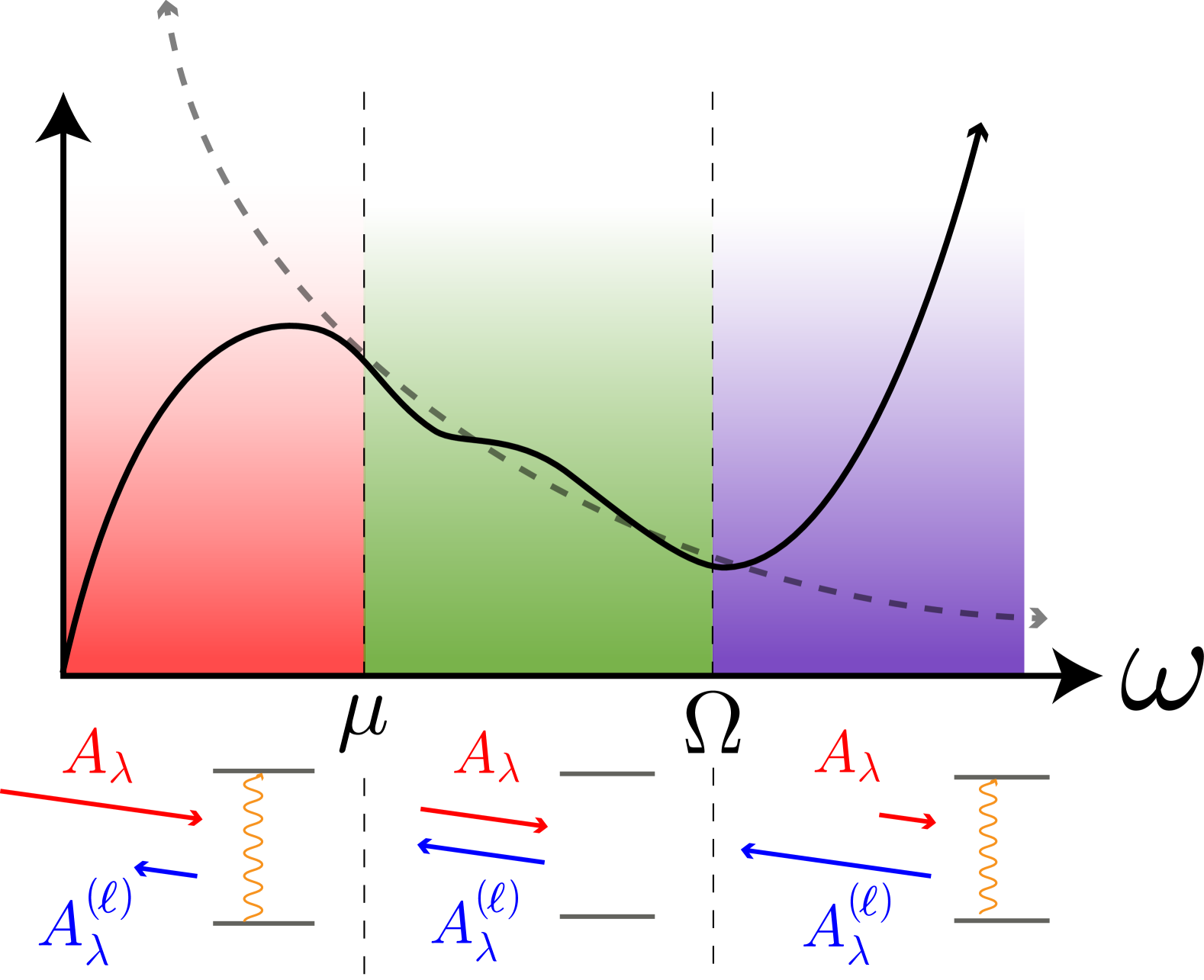
Observe that in Eq. (9) all of the information about the particular system enters via the spectral function . For a universal CD protocol we would like to develop a variational procedure which is independent of the details of the system. To do this, we will replace the exact spectral function with the following rectangular function:
| (11) |
Here is the low-frequency cutoff, which plays the same role as the cutoff in the filter function , so we keep the same notation. It determines the lowest frequency scale below which the approximate AGP does not follow the exact one. Likewise, the scale plays the role of the upper frequency cutoff. Clearly, the universal variational AGP construction converges if by increasing the order of approximation we are able to decrease the low frequency while keeping sufficiently large such that the exact cost function (9) remains small. The advantage of the universal approach is that the information about the system only enters through the scaling of the exact spectral function in the limits and , which in turn determine the scaling of the error with . The variational optimization becomes a purely mathematical problem of fitting the function by odd polynomials in , within the range . This procedure is schematically illustrated in Figure 1. The local CD protocol does not suppress transitions to the states with and conversely induces transitions at . After the optimal fitting in this window is achieved the parameters and have to be optimized for each . In this way the number of independent variational parameters is reduced from to only two.
The expansion for the AGP in Eq. (6) in terms of nested commutators leads to the polynomial approximation of the function as it is evident from Eq. (9). It is more convenient instead to use an expansion in different polynomials. The reason is that the monomials of Eq. (7) are difficult to work with numerically due to the exponential growth of the coefficients . In the direct variational approach it is more convenient to work with orthogonal operators forming a Krylov space Sels and Polkovnikov (2023b); Bhattacharjee (2023); Takahashi and Del Campo (2024). It is straightforward to check that this procedure is equivalent to an approximation of in Eq. (9) in terms of polynomials which are orthogonal with respect to the spectral function , which depends on the details of the system. Thus it is not suitable for a universal protocol. Instead we replace Eq. (6) with a linear combination of model independent orthogonal polynomials. In this work we consider an expansion in terms of Chebyshev polynomials . We rescale the frequency because the Chebyshev polynomials are well-behaved and orthogonal in the interval with the weight function Trefethen (2019). In the operator language this expansion corresponds to replacing the ansatz (6) with an equivalent one:
| (12) |
where stands for the Liouvillian super-operator: . It is clear that the set of coefficients and are uniquely related for any . More detail about this construction is given in Appendix B.
For the universal ansatz we optimize the cost function (9), where we replace the true spectral function with the rectangular one (11). This means that we have cast the problem as choosing the coefficients which minimize the following cost function
| (13) |
where plays the role of and . Here we have also replaced since the regularization is now provided by the lower cutoff . For fixed values of and we can now minimize Eq. (13) with respect to the coefficients and plug them into (12) to find the local ansatz for the AGP. For each , this depends on two parameters: and . Then, all that remains is to find an optimal way to choose them.
An accurate polynomial approximation of in the interval ensures that the main contributions to Eq. (9) comes from the regions and . The first, low frequency contribution is determined by the minimum gap, and more generally by the density of the low-energy states. If optimal value of is a monotonically decreasing function of , the low frequency contribution is suppressed more and more as . The latter, high frequency contribution is clearly determined by the high frequency tail of , which, in the thermodynamic limit, is typically given by
| (14) |
It has been rigorously proven for systems with a bounded local Hilbert space such as spins or lattice fermions, which satisfy Lieb-Robinson bounds, that Abanin et al. (2015). It was further conjectured that for generic systems, finite temperature spectral functions saturate the bound Parker et al. (2019), with an additional logarithmic correction in one-dimensional systems Avdoshkin and Dymarsky (2020). Similar exponential scaling of was numerically observed for generic classical systems (both integrable and chaotic) with an unbounded spectrum Lim et al. (2024).
The remainder of this work will be concerned with how the two parameters and for the optimal protocol scale with the order of approximation . As we shall see, not only , but surprisingly also depends strongly on the exponent : for the universal protocol does not exist in the thermodynamic limit in the sense that the UV error introduced by using higher order polynomials is too big to allow for to decrease with . Conversely for the universal protocol works such that is a decreasing with . The generic borderline case requires extra care and one can achieve very slow convergence Finžgar et al. (2025). In the remainder of this paper we will explain where this result comes from and illustrate the emerging scaling of and for three different situations.
II.2 Noninteracting models
Let us first consider the case of a many-body system which may be reduced to a system of free particles with a bounded single-particle spectrum. These models, for example, are naturally realized in lattice systems within the tight-binding approximation. In this case, there is a maximum excitation energy beyond which all matrix elements of local single-particle operators are identically equal to zero: for . It is then clear that we can set the upper cutoff irrespective of and never worry about accuracy of the polynomial fit of above this scale. Because is independent of we only need to optimize for , and hence find the optimal .
As a specific example, we choose the transverse field Ising (TFI) model, which is exactly solvable by mapping to free fermions via the Jordan-Wigner transformation Jordan and Wigner (1928). The protocol is to anneal from the ground state in the paramagnetic phase to the ferromagnetic phase. This is encoded in the following Hamiltonian
| (15) |
where tuning from 0 to 1 induces this phase transition. In this model, , and we take so that .
We can choose the low frequency cutoff so that the final state fidelity of the universal protocol
| (16) |
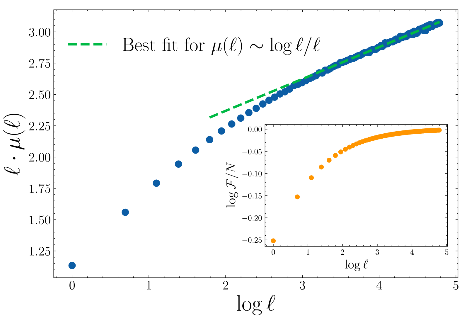
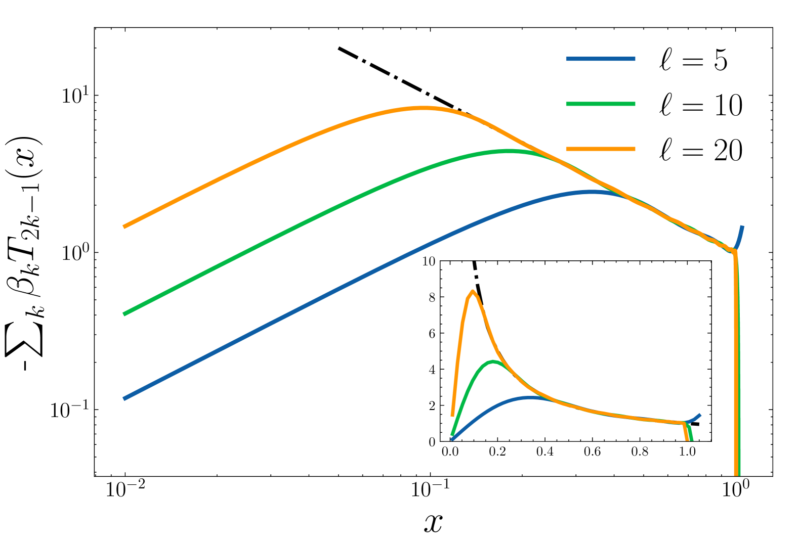
is maximized, where is the state evolved by in Eq. (1) with the approximate AGP obtained by the polynomial fitting method, and is the ground state of . Because this model consists of free particles, the fidelity may be calculated directly in the thermodynamic limit where finite size effects are not a concern. We then numerically optimize this fidelity with respect to for a fixed , which in turn determines the variational coefficients as they depend implicitly on through the cost function. We then find the asymptotic scaling , shown in Figure 2. The resulting fits to for a few values of are shown in Fig. 3. Instead of maximizing the fidelity one can use rigorous mathematical results for polynomial approximation of using the cost function in Eq. (13) within a finite window Childs et al. (2017) and arrive at the same asymptotic result.
Once the optimal value of the ratio
| (17) |
together with the coefficients , are fixed by using the test TFI model, the only remaining scale to be optimized for general models is the UV cutoff . In Sec. III we will do this optimization numerically, again using the fidelity (16). However, as we discuss next, one can understand the asymptotic behavior of (and hence of ) analytically using only the high frequency scaling of the spectral function (14). We highlight again that the TFI model here serves merely as a means of finding a universal protocol up to an overall scale .
II.3 Interacting Models & Asymptotes of the Spectral Function
For single-particle models, where there are no excitations above a certain maximum, this method is guaranteed to converge since for constant , clearly . Thus, the interval such that the universal protocol will asymptotically suppress more and more low-energy excitations with increasing without exciting any high-frequency modes. In general, the convergence of the universal protocol with is guaranteed as long as grows slower than . In this case we still have .
For a generic interacting model we can estimate the scaling from the requirement that the UV part of the cost function does not increase with (9). At high frequencies this part is dominated by the highest order polynomial so we can estimate
| (18) |
where we assumed that Eq. (14) holds at sufficiently large frequencies. The condition that thus requires that
| (19) |
Note that in one-dimensional models, asymptotically the spectral function has an extra logarithmic correction Avdoshkin and Dymarsky (2020): . It is easy to see that this correction modifies Eq. (19) to .
We see that in order to control the UV error of the cost function we should choose to be at least as the bound given by Eq. (19). As a result using Eq. (17) and ignoring for simplicity logarithmic corrections we arrive at the scaling
| (20) |
Physically, this result means that for the error in approximating the AGP, which results in high energy excitations, is very large unless increases very quickly with . In turn, this requisite rapid increase while keeping a fixed ratio does not allow decreasing , so that the local protocol will not suppress low-energy, non-adiabatic transitions at large . Conversely for the necessary increase of to control the UV error is sufficiently slow such that decreases and the local CD protocol works better and better with increasing .
Summarizing our discussion here we arrive at the most surprising conclusion in this work, tying the complexity of local CD protocols to the high frequency properties of the system. This happens despite the fact that when constructing counterdiabatic protocols, we are typically interested in suppressing the low energy excitations in the system (which set the norm of the exact AGP). The same low energy excitations determine the minimal protocol time in conventional quantum annealing schemes. For example, if we analyze driving across a critical point, such low-energy excitations get “frozen out” in the Kibble-Zurek mechanism Zurek (1985); Polkovnikov (2005); Dziarmaga (2005); Zurek et al. (2005). The scaling (20) states that contrary to these expectations, performance of the local CD protocol – at least in the Krylov space – is tied to the high frequency response of the system. This suggests there is some fundamental connection between the short- and long-time dynamics as alluded to earlier.
Note that our results are asymptotic in nature and do not imply that approximate CD driving cannot lead to significant improvements in fidelity at finite orders . There are many examples in the literature showing that this is the case in various interacting models, both quantum and classical. Also, for finite systems the spectral function generally saturates at , where is the system size, suggesting that even for the generic case the performance of local CD protocols will inevitably start improving for .
III Constructing Universal Protocols for Specific Systems
We will now discuss three separate models, each with different high-frequency behavior of the spectral function. i) The noninteracting transverse field Ising model with disorder, which has a high frequency hard cutoff; ii) a generic interacting model with approximately exponential () high frequency tail of the spectral function (modulo log-correction) and; iii) an interacting integrable model which has an approximately Gaussian high frequency tail corresponding to .
III.1 Transverse Field Ising Model with Modulated Fields
To test our universal protocol, we introduce disorder in the fields of the TFI model, which retains the paramagnetic to ferromagnetic transition present in the clean model Fisher (1992). Instead of analyzing a fully disordered model, we split the spin chain into contiguous blocks , each of size . There is random disorder within each block, which is repeated over the lattice. The Hamiltonian is
| (21) |
with drawn uniformly between and with . This will increase the size of the blocks in momentum space after the Jordan-Wigner transformation, but the blocks remain small enough that the dynamics may be computed via exact diagonalization.
The presence of randomness does not affect the maximum single particle energy, which remains so we again choose .
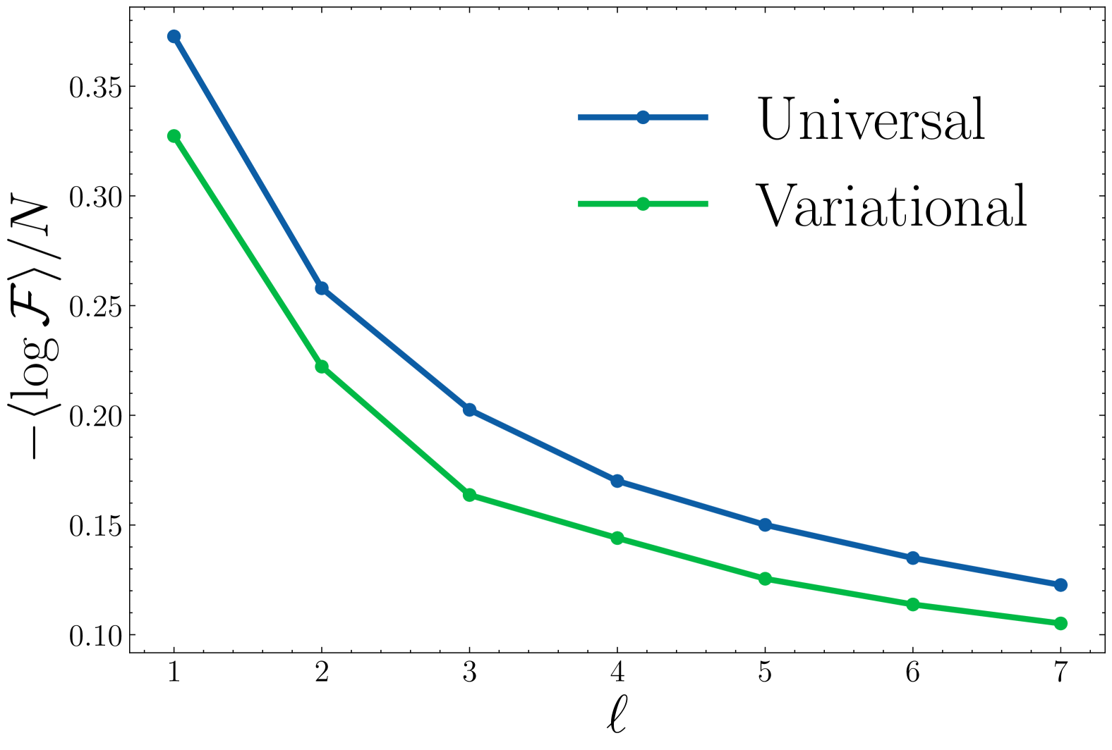
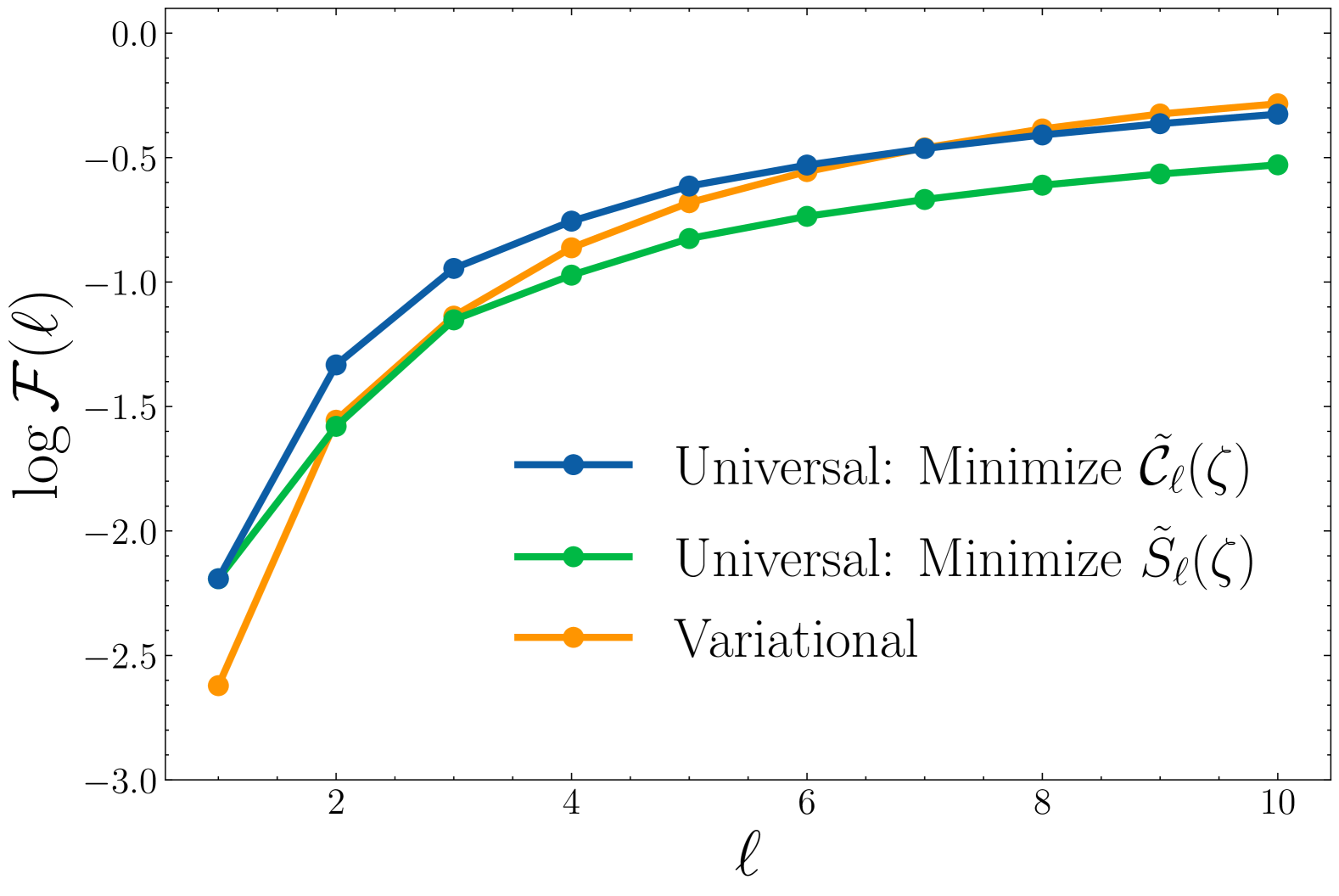
Using found for the non-disordered TFI model, with the large asymptote given by Eq. (17), we show in Figure 4 the results of the protocol obtained for the clean model applied to this model. Despite having no knowledge of the specific details of the disorder present in the system, the fidelity density in the thermodynamic limit improves at a rate similar to the variational approach.
III.2 Ising Model with Next-Nearest-Neighbor Interactions
Next we move to analysis of a generic nonintegrable system by adding next-nearest-neighbor interactions to the (clean) TFI model. This corresponds to driving the following Hamiltonian:
| (22) |
where we take , which will retain the same transition, albeit at a different value of Suzuki et al. (2013).
From our discussion in Section II.3, for generic one-dimensional systems, one expects an asymptotic linear scaling of the UV cutoff: . In Figure 5 we show the scaling of obtained by choosing it to maximize the final state fidelity at fixed . We find very good agreement with that prediction.
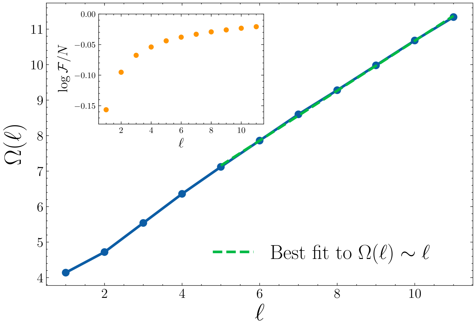
With the scaling of from Eq. (17), this linear growth of gives . So the infrared cutoff, instead of decreasing, slowly increases with . We therefore conclude that in the thermodynamic limit the universal protocol, and more generally the Krylov space variational ansatz for the AGP does not converge. Notice though that the universal protocol still leads to a significant improvement of fidelity at finite .
III.3 XXZ Model
It was conjectured that certain non-generic interacting integrable models can have slower operator growth than generic ones, and hence have a faster-than-exponential decay of the spectral function Parker et al. (2019). In particular, there is numerical evidence of Gaussian decay, corresponding to in Eq. (14), for the XXZ model Elsayed et al. (2014); LeBlond et al. (2019). In Appendix C, we provide further numerical evidence confirming this decay by looking at the growth of Lanczos coefficients. To test the scaling of in this case we now analyze this model using the following annealing Hamiltonian:
| (23) |
where . We take , so that we are annealing from the Heisenberg point to a pure Ising point.
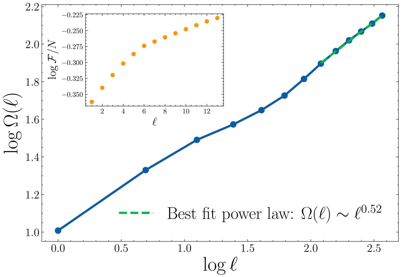
The scaling argument from Sec. II.3 for gives up to log-corrections. In Figure 6, we show that the same approach of choosing with fixed to maximize the final state fidelity indeed quite accurately reproduces this scaling. In turn, from Eq. (20) we see that , suggesting that the fidelity of the universal protocol should be improving with increasing as is evident from the inset in Fig. 6.
IV Summary & Outlook
Exact CD driving allows for adiabatic state preparation at arbitrarily fast speeds. By relaxing the condition on perfect state preparation, we can obtain approximate fast control protocols which are tractable. It is natural to construct the variational basis for these approximate protocols in Krylov space. Then, problem of finding approximate control protocols is entirely equivalent to approximating the function by odd polynomials in . All information about the system only enters through the spectral function of the operator .
In this work we minimize this distance using a fixed Chebyshev polynomial approximation of in a finite window , where and is the order of the polynomial. Then we use an overall energy scale , which rescales this interval to where , as the single remaining variational parameter. We find that its asymptotic dependence on is determined by the scaling of the high-frequency tail of the spectral function. In particular, if these tails decay faster than exponentially with frequency, the universal protocol is guaranteed to improve with even in the thermodynamic limit. However, in generic situations, where these tails are expected to be exponential, we find that the scale needs to grow linearly with so that the lower cutoff saturates at a finite value. This saturation prevents an approximate CD protocol from continuously improving with in the thermodynamic limit.
These protocols perform comparably with variational approaches that require knowledge of the Hamiltonian beforehand. Along the way, we discover a very interesting connection between the low- and high-frequency response of a system.
There are several further improvements to this method that might be made. For example, the high-frequency tail of the spectral function usually converges quickly with the system size, such that one could compute this efficiently for small systems and extrapolate to the thermodynamic limit. Then one can use this extrapolated spectral function as a weight function in the polynomial fitting of and additionally improve convergence of the approximate CD protocol Finžgar et al. (2025).
Interestingly, the results of this work show that one can search for optimal annealing paths amenable to local CD driving by minimizing high-frequency tails of the spectral function and hence minimizing high-frequency noise and dissipation. These paths should be most suitable for fast adiabatic state preparation. This finding suggests existence of some fundamental connections between short- and long-time response of interacting systems and needs further exploration. Lastly, this method might be fruitfully applied to practical quantum annealing where the problem Hamiltonian, or a model for the disorder/noise, is not exactly known.
Note: In the latter stages of this project, the authors became aware of another work in progress [Finžgar et al., 2025] which arrives at similar results via different means. These works have been submitted simultaneously.
Acknowledgments
The authors thank Dries Sels for many beneficial discussions, and John Martyn for information on rigorous results in polynomial approximation. This work was supported by the AFOSR Grant FA9550-21-1-0342. The exact code used is available online 333See https://github.com/smorawetz/CD-extra-controls.git.
Appendix A Extra factor of in cost function
As described in the main text, the established variational principle involves minimizing the action defined in Eq. (5). Writing this explicitly in terms of matrix elements and then employing the definition of the spectral function in Eq. (4) gives
| (24) |
This expression differs from the cost function that is used in this work, defined in Eq. (9), by a factor of in the brackets. To assess the effect of this factor, we repeat the same analysis as in the main text by using the dimensionless action
| (25) |
instead of the cost function (13) and repeat the same steps as in the main text. This procedure results in a slightly different and due to modified integrand. We compare the final state fidelity for the NNN TFI model annealing protocol using this approach with that of the main text in Figure 7, and find the difference is minimal.
Appendix B Constructing the AGP in terms of Chebyshev polynomials
The Chebyshev polynomials , where are defined using the following recursive relation:
Then one can always uniquely represent
| (26) |
In the corresponding operator construction (12) rescaling of , is equivalent to rescaling the Hamiltonian appearing in the Liouvillian by . With this, the coefficients then correspond to representing the AGP in terms of the operators defined as
in the following way:
| (27) |
We then obtain the by substituting picking the to minimize in Eq. (13).
Appendix C Numerical evidence of spectral function Gaussian decay in XXZ Model
The asymptotic growth of the so-called Lanczos coefficients is related to the high-frequency tail of the spectral function Parker et al. (2019) by the relation
| (28) |
with the presence of logarithmic corrections in one dimension. Thus, in order to establish Gaussian decay of the spectral function, we can look at the asymptotic growth of the Lanczos coefficients.
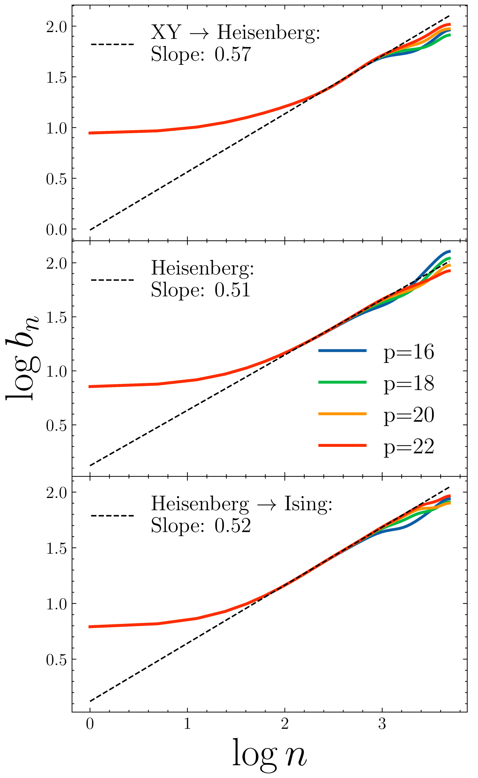
Using a recently developed Julia package leveraging the Pauli string structure of spin-1/2 models Loizeau et al. (2024), we can compute these Lanczos coefficients for very large systems. Although has been observed several times at the Heisenberg point, the growth at other nearby points has not been studied. We reparametrize the XXZ model as
| (29) |
We will examine the growth of Lanczos coefficients for , (the Heisenberg point) and . These are shown in Figure 8. We see for and the growth agrees well with . For there is a noticeable deviation from , which could be a finite size effect. To avoid dealing with this, for the numerics in the main text, we choose to anneal from the Heisenberg point to a regime of strong anisotropy () as described.
References
- Aidelsburger et al. (2013) M. Aidelsburger, M. Atala, M. Lohse, J. T. Barreiro, B. Paredes, and I. Bloch, Physical Review Letters 111, 185301 (2013).
- Gross and Bloch (2017) C. Gross and I. Bloch, Science 357, 995 (2017).
- Ebadi et al. (2021) S. Ebadi, T. T. Wang, H. Levine, A. Keesling, G. Semeghini, A. Omran, D. Bluvstein, R. Samajdar, H. Pichler, W. W. Ho, S. Choi, S. Sachdev, M. Greiner, V. Vuletić, and M. D. Lukin, Nature 595, 227 (2021).
- Friis et al. (2018) N. Friis, O. Marty, C. Maier, C. Hempel, M. Holzäpfel, P. Jurcevic, M. B. Plenio, M. Huber, C. Roos, R. Blatt, and B. Lanyon, Physical Review X 8, 021012 (2018).
- Zhang et al. (2017) J. Zhang, G. Pagano, P. W. Hess, A. Kyprianidis, P. Becker, H. Kaplan, A. V. Gorshkov, Z.-X. Gong, and C. Monroe, Nature 551, 601 (2017).
- Barends et al. (2016) R. Barends, A. Shabani, L. Lamata, J. Kelly, A. Mezzacapo, U. L. Heras, R. Babbush, A. G. Fowler, B. Campbell, Y. Chen, Z. Chen, B. Chiaro, A. Dunsworth, E. Jeffrey, E. Lucero, A. Megrant, J. Y. Mutus, M. Neeley, C. Neill, P. J. J. O’Malley, C. Quintana, P. Roushan, D. Sank, A. Vainsencher, J. Wenner, T. C. White, E. Solano, H. Neven, and J. M. Martinis, Nature 534, 222 (2016).
- Ma et al. (2019) R. Ma, B. Saxberg, C. Owens, N. Leung, Y. Lu, J. Simon, and D. I. Schuster, Nature 566, 51 (2019).
- Eickbusch et al. (2022) A. Eickbusch, V. Sivak, A. Z. Ding, S. S. Elder, S. R. Jha, J. Venkatraman, B. Royer, S. M. Girvin, R. J. Schoelkopf, and M. H. Devoret, Nature Physics 18, 1464 (2022).
- Google Quantum AI (2023) Google Quantum AI, Nature 614, 676 (2023).
- King et al. (2023) A. D. King, J. Raymond, T. Lanting, R. Harris, A. Zucca, F. Altomare, A. J. Berkley, K. Boothby, S. Ejtemaee, C. Enderud, E. Hoskinson, S. Huang, E. Ladizinsky, A. J. R. MacDonald, G. Marsden, R. Molavi, T. Oh, G. Poulin-Lamarre, M. Reis, C. Rich, Y. Sato, N. Tsai, M. Volkmann, J. D. Whittaker, J. Yao, A. W. Sandvik, and M. H. Amin, Nature 617, 61 (2023).
- Henriet et al. (2020) L. Henriet, L. Beguin, A. Signoles, T. Lahaye, A. Browaeys, G.-O. Reymond, and C. Jurczak, Quantum 4, 327 (2020), arXiv:2006.12326 [quant-ph] .
- Haffner et al. (2008) H. Haffner, C. Roos, and R. Blatt, Physics Reports 469, 155 (2008).
- Kjaergaard et al. (2020) M. Kjaergaard, M. E. Schwartz, J. Braumüller, P. Krantz, J. I.-J. Wang, S. Gustavsson, and W. D. Oliver, Annual Review of Condensed Matter Physics 11, 369 (2020).
- Albash and Lidar (2018) T. Albash and D. A. Lidar, Reviews of Modern Physics 90, 015002 (2018).
- Guéry-Odelin et al. (2019) D. Guéry-Odelin, A. Ruschhaupt, A. Kiely, E. Torrontegui, S. Martínez-Garaot, and J. G. Muga, Rev. Mod. Phys. 91, 045001 (2019).
- Demirplak and Rice (2003) M. Demirplak and S. A. Rice, The Journal of Physical Chemistry A 107, 9937 (2003).
- Demirplak and Rice (2005) M. Demirplak and S. A. Rice, The Journal of Physical Chemistry B 109, 6838 (2005).
- Berry (2009) M. V. Berry, Journal of Physics A: Mathematical and Theoretical 42, 365303 (2009).
- del Campo (2013) A. del Campo, Physical Review Letters 111, 100502 (2013).
- Sels and Polkovnikov (2017) D. Sels and A. Polkovnikov, Proceedings of the National Academy of Sciences 114 (2017), 10.1073/pnas.1619826114.
- Claeys et al. (2019) P. W. Claeys, M. Pandey, D. Sels, and A. Polkovnikov, Physical Review Letters 123, 090602 (2019), arXiv:1904.03209 .
- Gjonbalaj et al. (2022) N. O. Gjonbalaj, D. K. Campbell, and A. Polkovnikov, Physical Review E 106, 014131 (2022), arXiv:2112.02422 [cond-mat, physics:quant-ph] .
- Čepaitė et al. (2023) I. Čepaitė, A. Polkovnikov, A. J. Daley, and C. W. Duncan, PRX Quantum 4, 010312 (2023).
- Schindler and Bukov (2024) P. M. Schindler and M. Bukov, Physical Review Letters 133, 123402 (2024).
- Duncan (2024) C. W. Duncan, Physical Review B 109, 245421 (2024).
- Morawetz and Polkovnikov (2024) S. Morawetz and A. Polkovnikov, Physical Review B 110, 024304 (2024).
- Van Vreumingen (2024) D. Van Vreumingen, Physical Review A 110, 052419 (2024).
- Gjonbalaj et al. (2025) N. O. Gjonbalaj, R. Sahay, and S. F. Yelin, “Shortcuts to Analog Preparation of Non-Equilibrium Quantum Lakes,” (2025), arXiv:2502.03518 [quant-ph] .
- Du et al. (2016) Y.-X. Du, Z.-T. Liang, Y.-C. Li, X.-X. Yue, Q.-X. Lv, W. Huang, X. Chen, H. Yan, and S.-L. Zhu, Nature Communications 7, 12479 (2016).
- An et al. (2016) S. An, D. Lv, A. Del Campo, and K. Kim, Nature Communications 7, 12999 (2016).
- Hu et al. (2018) C.-K. Hu, J.-M. Cui, A. C. Santos, Y.-F. Huang, M. S. Sarandy, C.-F. Li, and G.-C. Guo, Optics Letters 43, 3136 (2018).
- Boyers et al. (2019) E. Boyers, M. Pandey, D. K. Campbell, A. Polkovnikov, D. Sels, and A. O. Sushkov, Physical Review A 100, 012341 (2019).
- Bukov et al. (2019) M. Bukov, D. Sels, and A. Polkovnikov, Physical Review X 9 (2019), 10.1103/physrevx.9.011034.
- Pandey et al. (2020) M. Pandey, P. W. Claeys, D. K. Campbell, A. Polkovnikov, and D. Sels, Physical Review X 10 (2020), 10.1103/physrevx.10.041017.
- Bhattacharjee (2023) B. Bhattacharjee, “A Lanczos approach to the Adiabatic Gauge Potential,” (2023), arXiv:2302.07228 .
- Takahashi and Del Campo (2024) K. Takahashi and A. Del Campo, Physical Review X 14, 011032 (2024).
- Sakurai and Napolitano (2017) J. J. Sakurai and J. Napolitano, Modern Quantum Mechanics (Cambridge University Press, 2017).
- Kolodrubetz et al. (2017) M. Kolodrubetz, D. Sels, P. Mehta, and A. Polkovnikov, Physics Reports 697, 1 (2017), arXiv:1602.01062 [cond-mat] .
- Lim et al. (2024) C. Lim, K. Matirko, H. Kim, A. Polkovnikov, and M. O. Flynn, “Defining classical and quantum chaos through adiabatic transformations,” (2024), arXiv:2401.01927 [cond-mat.stat-mech] .
- Note (1) It is straightforward to check that extra term in the action leads to the same regularization of the AGP as in Eq. (2).
- Sels and Polkovnikov (2023a) D. Sels and A. Polkovnikov, Physical Review X 13 (2023a), 10.1103/physrevx.13.011041.
- Bukov et al. (2015) M. Bukov, L. D’Alessio, and A. Polkovnikov, Advances in Physics 64, 139 (2015).
- Goldman and Dalibard (2014) N. Goldman and J. Dalibard, Physical Review X 4, 031027 (2014).
- Choi et al. (2020) J. Choi, H. Zhou, H. S. Knowles, R. Landig, S. Choi, and M. D. Lukin, Physical Review X 10, 031002 (2020).
- Note (2) If we are only interested in the ground state CD we can set .
- Sels and Polkovnikov (2023b) D. Sels and A. Polkovnikov, Physical Review X 13, 011041 (2023b).
- Trefethen (2019) L. N. Trefethen, Approximation Theory and Approximation Practice, Extended Edition (Society for Industrial and Applied Mathematics, 2019).
- Abanin et al. (2015) D. A. Abanin, W. De Roeck, and F. Huveneers, Physical Review Letters 115, 256803 (2015).
- Parker et al. (2019) D. E. Parker, X. Cao, A. Avdoshkin, T. Scaffidi, and E. Altman, Physical Review X 9, 041017 (2019), arXiv:1812.08657 [cond-mat, physics:hep-th, physics:nlin, physics:quant-ph] .
- Avdoshkin and Dymarsky (2020) A. Avdoshkin and A. Dymarsky, Physical Review Research 2, 043234 (2020).
- Finžgar et al. (2025) J. R. Finžgar, S. Notarnicola, M. Cain, M. D. Lukin, and D. Sels, “Universal counterdiabatic driving with performance guarantees,” (2025).
- Jordan and Wigner (1928) P. Jordan and E. Wigner, Zeitschrift für Physik 47, 631 (1928).
- Childs et al. (2017) A. M. Childs, R. Kothari, and R. D. Somma, SIAM Journal on Computing 46, 1920 (2017), arXiv:1511.02306 [quant-ph] .
- Zurek (1985) W. H. Zurek, Nature 317, 505 (1985).
- Polkovnikov (2005) A. Polkovnikov, Physical Review B 72 (2005), 10.1103/physrevb.72.161201.
- Dziarmaga (2005) J. Dziarmaga, Physical Review Letters 95 (2005), 10.1103/physrevlett.95.245701.
- Zurek et al. (2005) W. H. Zurek, U. Dorner, and P. Zoller, Physical Review Letters 95 (2005), 10.1103/physrevlett.95.105701.
- Fisher (1992) D. S. Fisher, Physical Review Letters 69, 534 (1992).
- Suzuki et al. (2013) S. Suzuki, J.-i. Inoue, and B. K. Chakrabarti, Quantum Ising Phases and Transitions in Transverse Ising Models, Lecture Notes in Physics, Vol. 862 (Springer Berlin Heidelberg, Berlin, Heidelberg, 2013).
- Elsayed et al. (2014) T. A. Elsayed, B. Hess, and B. V. Fine, “Signatures of Chaos in Time Series Generated by Many-Spin Systems at High Temperatures,” (2014), arXiv:1105.4575 .
- LeBlond et al. (2019) T. LeBlond, K. Mallayya, L. Vidmar, and M. Rigol, “Entanglement and matrix elements of observables in interacting integrable systems,” (2019), arXiv:1909.09654 .
- Note (3) See https://github.com/smorawetz/CD-extra-controls.git.
- Loizeau et al. (2024) N. Loizeau, J. C. Peacock, and D. Sels, “Quantum many-body simulations with PauliStrings.jl,” (2024), arXiv:2410.09654 [quant-ph] .