Inverse bubbles from broken supersymmetry

Abstract

Building upon the recent findings regarding inverse phase transitions in the early universe, we present the first natural realisation of this phenomenon within a supersymmetry-breaking sector. We demonstrate that inverse hydrodynamics, which is characterized by the fluid being aspirated by the bubble wall rather than being pushed or dragged, is actually not limited to a phase of (re)heating but can also occur within the standard cooling cosmology. Through a numerical analysis of the phase transition, we establish a simple and generic criterion to determine its hydrodynamics based on the generalised pseudo-trace. Our results provide a proof of principle highlighting the need to account for these new fluid solutions when considering cosmological phase transitions and their phenomenological implications.

Introduction – Phase transitions (PTs) in the early universe plasma, usually called cosmological phase transitions, are fascinating phenomena. First order PTs (FOPTs) proceeding via the nucleation and expansion of bubbles of the true vacuum inside a sea of false vacuum are of particular interest as they can be at the origin of the matter-antimatter asymmetry of the universe (baryogenesis) [1, 2, 3, 4, 5, 6, 7, 8, 9, 10, 11, 12, 13, 14], lead to the production of dark matter [15, 16, 17, 18, 19, 20, 21, 22, 23, 24, 25, 26, 27] and primordial black holes [28, 29, 30, 31, 32], and can be a powerful source of primordial gravitational waves (GWs) as well [33, 34, 35, 36, 37]. The broad program to discover and investigate a possible background of GWs by current experiments such as Ligo–Virgo–Kagra [38] and Pulsar Timing Arrays [39], as well as future detectors such as the LISA [40] and the Einstein Telescope [41], opens the unique opportunity of probing the existence of FOPTs and of new fundamental physics. Indeed, FOPTs appear naturally in a large variety of scenarios beyond the Standard Model (BSM) like composite Higgs [42, 43, 44, 45, 46], extended Higgs sectors [47, 48, 49, 50, 51, 52, 53, 54], axion models [55, 56], dark Yang-Mills sectors [57, 58], $B-L$ breaking sectors [59, 60] and SUSY breaking sectors [61, 62], and may also be catalyzed by impurities in the early universe, see e.g. [63, 64, 65, 66, 67, 68, 69, 70, 71, 72, 73, 74, 75], as well as occur in the core of neutron stars [69, 76, 77, 78].

The dynamics of FOPTs involve a non–trivial interplay between the bubble wall and the surrounding plasma, which is pivotal in determining the phenomenology of the PT including the GW emission. The hydrodynamical modes describing the bulk fluid motion in the background of an expanding bubble during a direct FOPT have been classified a long time ago [79, 80, 81, 82]: they consist of detonations and deflagrations, together with a class of hybrid modes interpolating between the two. For all these solutions, the fluid is either dragged or pushed by the bubble wall. The bulk fluid velocity is then always aligned with the wall velocity in the plasma frame. In the case of the so–called inverse PTs, the plasma is instead aspirated inside the expanding bubble and the fluid flows in the opposite direction of the bubble wall motion in the plasma frame [83, 84]. These solutions have been so far studied in the context of a (re)heating PT [85, 83, 84], where the temperature of the system increases with time, and thus have been associated to superheated bubbles, see also [86, 87].

In this paper, we show that inverse hydrodynamics is actually not limited to the heating scenario mentioned above, but can instead take place during the standard cooling of the universe, for instance during radiation domination. Interestingly, we find the emergence of this novel hydrodynamics in the context of supersymmetry (SUSY) and $R$–symmetry breaking. In particular, the PT along the pseudomodulus direction within the minimal O’Raifeartaigh model for spontaneous SUSY breaking turns out to be inverse in a relevant part of its parameter space. As we shall see, the occurrence of inverse bubbles can be traced back to the properties of the SUSY spectrum and its distinctive thermal history, opening the possibility of testing these properties through their imprint on the PT and the corresponding GWs. We also provide a precise characterisation of the inverseness of a FOPT by providing a simple criterion based on the sign of a generalised pseudo-trace to readily discriminate between direct and inverse FOPTs. Our findings extend the understanding of inverse phase transitions and their phenomenological implications, offering new avenues for studying their impact on gravitational wave signatures and beyond.

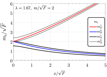
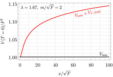
Figure 1: Left panel: Mass spectrum of the SUSY-breaking sector. The fermionic mass eigenstates are shown in red and blue, while the scalar mass eigenstates are depicted in grey and black. The latter are split into pairs around the corresponding fermionic mass eigenstates. Right panel: Tree-level (black) and one-loop corrected (red) potential of the SUSY model along the pseudomodulus direction.

PTs in a SUSY breaking sector – Supersymmetry is not a symmetry of the low-energy theory. Therefore, if it is realised at high energy scales, it must be broken by a dedicated SUSY-breaking sector. A broad class of perturbative SUSY-breaking mechanisms can be described within the framework of an effective field theory that encapsulates the dynamics of the so-called pseudomodulus. This pseudomodulus corresponds to the scalar component $x$ of the chiral superfield, $X$, which is directly related to SUSY breaking

$${}X=\frac{x}{\sqrt{2}}e^{2ia/f_{a}}+\sqrt{2}\theta\tilde{G}+\theta^{2}F\,,$$ (1)

where we have used the standard superspace notation. A thorough characterisation of such PTs within different realisations of the SUSY breaking sector was provided in [62]. In our study, as a minimal benchmark model, we focus on the O’Raifeartaigh model [88]. In addition to the pseudo-modulus, the SUSY breaking sector contains four chiral superfields $\phi_{1},\tilde{\phi}_{1},\phi_{2},\tilde{\phi}_{2}$. The superpotential takes the form

$${}W=-FX+\lambda X\phi_{1}\tilde{\phi}_{2}+m(\phi_{1}\tilde{\phi}_{1}+\phi_{2}\tilde{\phi}_{2})\,.$$ (2)

The model in Eq.(2) preserves an $R-$symmetry, which typically accompanies dynamical SUSY breaking [89, 90] and under which $X$ has charge two, $R[X]=2$. The modulus $x$ thus serves as the order parameter governing the spontaneous breaking of the $R$-symmetry. The vacuum expectation values that minimize the tree–level potential are given by $\phi_{1}=\phi_{2}=\tilde{\phi}_{1}=\tilde{\phi}_{2}=0$, leading to a tree-level vacuum energy of $V^{\rm min}_{\rm tree}=|F|^{2}$. Consequently, the potential remains constant as a function of $x$ indicating that supersymmetry is broken irrespective of $x$, while $R$-symmetry is restored at the origin.

On the other hand, the mass spectrum plays a crucial role in shaping the behaviour of the potential for $x$ at the loop level. To analyse this, we diagonalise the scalar and fermion mass matrices, defined as follows

$${}\mathcal{M}^{2}_{S,ij}\equiv{1\over 2}\bigg{(}\frac{\partial^{2}V}{\partial\phi_{i}\partial\phi_{j}}\bigg{)}\,,\quad\mathcal{M}_{F,ij}\equiv{1\over 2}\bigg{(}\frac{\partial^{2}W}{\partial\phi_{i}\partial\phi_{j}}\bigg{)}\,.$$ (3)

The scalar mass eigenstates are split in pairs around the fermionic mass eigenstates, as we can see in the left panel of Fig.1. There are also light fields from the superfield $X$, corresponding to the pseudomodulus, $x$, the $R$–axion, $a$, and the goldstino, $\tilde{G}$, which will have an influence on the hydrodynamics as they contribute to the number of relativistic species in the plasma. In Appendix A, we present the computation of the effective potential. Due to the one-loop corrections, this acquires a global minimum at the origin, as we can see in the right panel of Fig.1. A remarkable property of this potential, which is a reflection of the underlying SUSY, is that even at one-loop level it remains extremely flat away from the origin.

However, finite temperature effects (described in Appendix A) break SUSY explicitly and can have a strong impact on the pseudomodulus effective potential. The typical thermal history of the minimal O’Raifeartaigh model considered here is then as follows [62, 93, 94]: at high temperatures, $T\gtrsim\sqrt{F}$, the system has a single vacuum state with $\langle x\rangle=0$. At lower temperatures, a new local minimum of the effective potential appears at relatively large field values, $\langle x\rangle/\sqrt{F}\gg 1$, which can become the true vacuum of the theory below a certain critical temperature, $T_{c}$. This state with broken $R$-symmetry will however become metastable and then eventually disappear at even lower temperatures, given that the only minimum at $T=0$ is at $\langle x\rangle=0$, as already shown in the right panel of Fig. 1.

Figure 2: The free energy difference between the $R$–symmetry breaking and preserving vacua as a function of the temperature. For $T>T_{c}$, the symmetric vacuum is the global one, while for $T<T_{c}$, the broken phase with $\langle x\rangle\neq 0$ becomes favoured. The nucleation temperature (dashed red line) is found to be close to the temperature where the barrier disappears, $T/\sqrt{F}\approx 0.66$. At lower temperatures, $T/\sqrt{F}\lesssim 0.6$, the $R$–symmetry preserving vacuum becomes again the global minimum. The condition $D\vartheta=0$ marks the change from direct to inverse hydrodynamics. The insets indicate a sketch of the free energy, including the position of the relevant vacua in the corresponding temperature range.

In Fig. 2 we present an example of such thermal history for a characteristic benchmark point with $m/\sqrt{F}=2$ and $\lambda=1.67$, by showing the free energy difference between the vacuum at $\langle x\rangle=0$ and $\langle x\rangle\neq 0$, for temperatures where they both exist and are classically stable. At $T=T_{c}$ the free energy difference changes sign indicating that the minimum with broken $R$–symmetry starts to be favoured, and the system can now tunnel from the $R$–symmetry preserving vacuum to this new phase. This PT is first order and is controlled by a thermal barrier that will eventually disappear at $T/\sqrt{F}\simeq 0.66$. Nucleation in the expanding universe will in fact take place at a slightly higher temperature, $T_{\text{nuc}}/\sqrt{F}\approx 0.665$, as evaluated numerically and shown by the dashed red line. As the system continues to cool, the barrier reappears, and the symmetry-breaking minimum is gradually lifted until it once again becomes degenerate with the origin at $T=T_{c,2}$. Finally, at very low temperatures, the symmetry breaking minimum disappears and the symmetry is restored again, causing a second FOPT.

In this paper, we will focus on the first transition that will take place in the expanding universe, namely the $R$–symmetry breaking FOPT towards the vacuum with $\langle x\rangle\neq 0$. As we shall see, this PT can actually proceed according to either the direct or the inverse hydrodynamics (see Ref. [83, 84]) depending on the microscopic coupling constant $\lambda$ entering the superpotential in Eq. (2) (while the second FOPT restoring $R$–symmetry will always be direct). This is shown in Fig. 3, where the nucleation temperature as a function of $\lambda$ is indicated by the red line (keeping $m/\sqrt{F}=2$ fixed). As we can see, for all points nucleation takes place very close to the temperature where the barrier actually disappears. For $\lambda\lesssim 1.63$, bubble nucleation occurs in the region where the hydrodynamics will be the one based on the direct detonation and deflagration type of solutions, while for $1.63\lesssim\lambda\lesssim 1.68$ the hydrodynamics will be inverse, as we shall discuss in detail in the next sections.

For each value of the coupling constant $\lambda$, we also evaluate numerically the duration of the FOPT compared to one Hubble time, obtaining typical values of $\beta/H=\mathcal{O}(10^{4})$, where as usual $\beta=-\frac{d}{dt}S_{3}/T$ and $S_{3}$ is the $O(3)$ bounce action (see Appendix B for more details).

Thermodynamics and hydrodynamics of the SUSY model – In the early universe, FOPTs can be modelled as the interplay between a scalar field $\phi$, whose vacuum expectation value represents the order parameter of the transition, and the surrounding plasma which is often well described by a relativistic fluid. The energy–momentum tensor of the system consists then of those two contributions, $T^{\mu\nu}=T^{\mu\nu}_{\text{fluid}}+T^{\mu\nu}_{\phi}$, with

$$T^{\mu\nu}_{\phi} =\partial^{\mu}\phi\partial^{\nu}\phi-g^{\mu\nu}\left(\frac{1}{2}(\partial\phi)^{2}-V(\phi)\right)$$ (4a)

$$T^{\mu\nu}_{\text{fluid}} =(e+p)u^{\mu}u^{\nu}-pg^{\mu\nu},$$ (4b)

where $u^{\mu}$ is the four-velocity of the fluid, $e$ is the energy density, $p$ is the pressure and $V(\phi)$ is the scalar potential. The pressure is related to the free energy as $p=-\mathcal{F}$, while the energy and enthalpy density are given by

$${}e=T\frac{dp}{dT}-p\,,\qquad w=e+p=T\frac{dp}{dT}\,.$$ (5)

In any particle physics model that can be solved (even if only approximately, e.g. in a loop expansion), the free energy $\mathcal{F}$ can be obtained directly from the effective potential at finite temperature, $V_{0}+V_{T}\equiv\mathcal{F}$. Consequently, the knowledge of the free energy of a given theory allows us to compute all the thermodynamic quantities of interest without introducing a simplified Equation of State (EoS) for the fluid, such as for instance the bag EoS and its generalizations.

The conservation of the energy–momentum tensor across the phase boundary, $\nabla_{\mu}T^{\mu\nu}=0$, gives the following junction conditions for the quantities that are discontinuous at the bubble wall

$$w_{+}\gamma_{+}^{2}v_{+} =w_{-}\gamma_{-}^{2}v_{-}\ ,$$ (6a)

$$w_{+}\gamma_{+}^{2}v_{+}^{2}+p_{+} =w_{-}\gamma_{-}^{2}v_{-}^{2}+p_{-}\ ,$$ (6b)

where the subscript “$\pm$” denotes quantities in front of/behind the phase boundary, so that for instance “$-$” always represents the interior of the bubble. To be explicit, $w_{+}=w_{s}(T_{+})$, $w_{-}=w_{b}(T_{-})$ (and similarly for $p_{\pm}$), where the label “$s/b$” denotes the symmetric/broken phase of the $R$–symmetry in the case of interest.

Upon rearranging the junction conditions, we arrive at the familiar relations for the fluid velocities ahead and behind the wall, the energies and the pressures

$${}v_{+}v_{-}=\frac{p_{+}-p_{-}}{e_{+}-e_{-}}\ ,\qquad\frac{v_{+}}{v_{-}}=\frac{e_{-}+p_{+}}{e_{+}+p_{-}}\ .$$ (7)

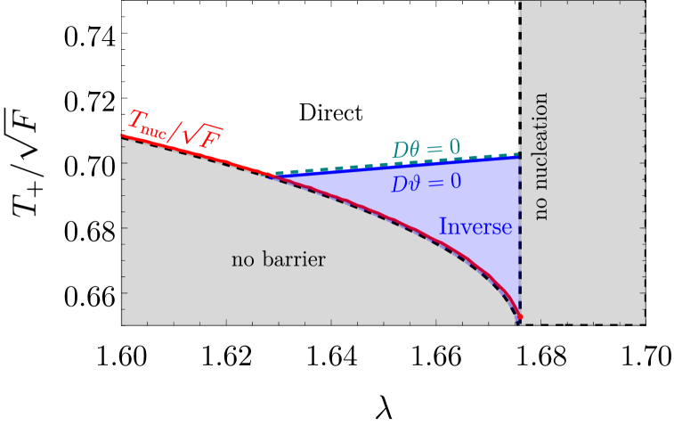
Figure 3: The nucleation temperature (red) is obtained as a function of $\lambda$ by numerically solving the condition $S_{3}/T=140$, which corresponds to setting $\sqrt{F}\sim$ TeV for concreteness. The blue-shaded region indicates the region of the inverse FOPTs, which occur approximately within the window $\lambda\in[1.63,1.675]$, while the white region indicates the parameter space where the FOPT will be direct. We also show the boundary between inverse and direct FOPTs according to the criteria $D\vartheta=0$ and $D\theta=0$, see discussion around Eq. (8), which agree well with the explicit evaluation of the hydrodynamics. For this figure we fixed $m/\sqrt{F}=2$.

Let us now examine the possible hydrodynamics of the $R$–symmetry breaking PT. The junction conditions above can be solved numerically by referring to the pressure and energy densities as evaluated directly from the free energy within our particle physics model. The allowed values for the $(v_{-},v_{+})$ pairs are shown in Fig. 4 for a representative benchmark point. The matching conditions in Eq. (7) are solved for $v_{\pm}$ in terms of the temperatures ahead and behind the wall, $T_{\pm}$. For consistency, we restrict $T_{+}$ to lie between $T_{c}$ and the temperature when the barrier disappears, $T_{\rm no\ barrier}$, as this is the range for which the FOPT can actually take place. The various $v_{\pm}$ trajectories in Fig. 4 are then shown together with the corresponding temperature $T_{+}$ according to the colour code. Because of the consistency condition on $T_{+}$ and the properties of our system free energy, the branches do not populate the entire $v_{\pm}\in(0,1)$ parameter space. The regions corresponding to inverse and direct hydrodynamics are indicated by solid and dashed lines, respectively. We find that these regions remain neatly separated across the entire $(v_{-},v_{+})$ plane, except for a small overlap in the regime of hybrid solutions (bottom-right corner). More details are presented in Appendix C. As a comparison, a similar discussion of the inverse branches in the case of the (template) $\mu\nu$-model is provided in Appendix D.

If we further specify the temperature of the FOPT as the one evaluated numerically from the bubble nucleation condition , we can select the bright red branch as the relevant one for this specific benchmark point . As we can see, the FOPT occurs in the inverse hydrodynamic regime, as anticipated in Fig. 3.

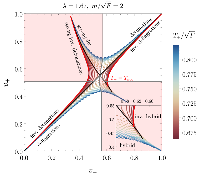
Figure 4: Possible solutions to the fluid matching conditions for $(v_{-},v_{+})$ for the $R$–symmetry breaking FOPT under consideration, plotting the relevant branches for different values of $T_{+}\in[T_{\rm no\ barrier},T_{c}]$. Dashed lines correspond to direct phase transitions, while solid lines indicate inverse transitions, determined by the sign of $\alpha_{\vartheta}$. The solid red line highlights the relevant branch at the nucleation temperature. The red-shaded area marks the region of strong (inverse) detonations and strong (inverse) deflagrations. In the bottom right corner, a zoomed-in view of the hybrid solution region reveals an overlap between different branches (see Appendix C for more details).

We defined inverse PTs as transitions displaying negative bulk velocities in the plasma frame: rather than being pushed outward, the surrounding plasma is drawn inward, effectively being aspirated into the expanding bubble. Let us now provide a sharper characterisation, or criterion, of inverse hydrodynamics which extends the intuitive one put forward in Ref. [83], according to which inverse PTs are found when the transition proceeds against the vacuum energy (namely, the $T=0$ effective potential for the order parameter). We find that a fully general characterization of inverse hydrodynamics can be obtained by defining a generalised pseudo-trace, $\alpha_{\vartheta}$, which extends the definition within the bag EoS adopted in  [83] as well as the pseudo-trace, $\alpha_{\theta}$, introduced in  [95]

$$\alpha_{\vartheta} \equiv\frac{4D\vartheta}{3w_{+}(T_{+})}\equiv\frac{4\left(De(T_{+})-\frac{\delta e}{\delta p}(T_{+},T_{-})Dp(T_{+})\right)}{3w_{+}(T_{+})},$$ (8)

where the $D$ and $\delta$ are defined as $Df=f_{+}(T_{+})-f_{-}(T_{+})$ and $\delta f=f_{-}(T_{+})-f_{-}(T_{-})$. For given values of $T_{\pm}$, which as discussed below (7) can be related to $v_{\pm}$ via the matching conditions, inverse hydrodynamics takes place for $\alpha_{\vartheta}<0$, while the standard one is realised for $\alpha_{\vartheta}>0$. This criterion is the one used to identify inverse and direct branches in Fig. 4. In this way, we discover that PTs proceeding against the vacuum energy can nonetheless display direct hydrodynamics.

Notice that for relatively weak PTs with $T_{+}\simeq T_{-}$, $\delta e/\delta p\simeq 1/c_{s,-}^{2}$, with $c_{s,-}$ being the speed of sound in the broken phase, and Eq. (8) reduces to $\alpha_{\theta}$ as defined in Ref. [95]. In the special case of a strictly constant speed of sound, this definition further reduces to $\alpha_{\theta}$ as derived in the template $\mu\nu$ model, see Eq. (52) in Appendix D. Finally, when the speed of sound is $c_{s}^{2}=1/3$ as for a relativistic gas, this definition reduces to $\alpha_{+}$ as considered in Ref. [83].

One can show that FOPTs with $\alpha_{\vartheta}=0$ represent the limit of weak hydrodynamics, where $\Delta e=0$ and $\Delta p=0$, with $\Delta f=f_{+}(T_{+})-f_{-}(T_{-})$. By continuity, this is supposed to separate inverse from direct PTs. This is confirmed by the results shown in Fig. 3, where the line of vanishing $\alpha_{\vartheta}$ actually corresponds to the boundary between direct and inverse regions, which are determined independently by solving the fluid equations. As we can see, the approximate condition in terms of the pseudo-trace, $\alpha_{\theta}=0$, reproduces this separation fairly well. This can be traced back to the fact that the speed of sound is not strongly temperature dependent in this model. We present the precise relation between the generalised pseudo-trace and the pseudo-trace in the $\mu\nu$ model in Appendix D.

Inverse fluid solutions for $R$–symmetry breaking – The hydrodynamics of inverse PTs was presented for the first time in Ref. [83, 84]. There exist five different possible expansion modes with negative bulk velocities [83, 96]: i) inverse detonations (weak and Chapman-Jouguet (CJ)), ii) inverse deflagrations (weak and CJ), and iii) inverse hybrids (see Fig.5). The inverse detonation (see left panel of Fig.5) is obtained by glueing a reaction front with $\xi_{w}=v_{-}<c_{s,-}$ and a rarefaction wave going from $v(\xi_{w}^{+})$ to $0$ at $\xi=c_{s,+}$. In the plasma frame, the velocity $v(\xi_{w}^{+})=\mu(v_{-},v_{+})$ with $v_{-}<v_{+}$ is always negative, where $\mu(v_{-},v_{+})=(v_{-}-v_{+})/(1-v_{-}v_{+})$ is the Lorentz transformed velocity. Notice however that since $\xi$ is positive the bubble is actually expanding. Across the rarefaction wave, namely from $\xi=c_{s,+}$ to $\xi=\xi_{w}$, the pressure as well as the velocity decreases.

The inverse deflagrations (see right panel of Fig.5) are obtained by glueing a reaction front with $v_{+}=\xi_{w}>v_{J,\rm inv}$, where $v_{J,\rm inv}$ is the inverse Jouguet velocity, and $v_{-}>c_{s,-}$ followed by a compression wave ending with a shock front.

Finally, in the regime between inverse detonations and inverse deflagration, for $c_{s,+}>\xi_{w}>v_{J,\rm inv}$ the steady state is an inverse hybrid (see middle panel of Fig.5). This solution consists of a rarefaction wave glued to a detonation front, followed by a compression wave and finally a shock wave. We can also define the largest possible window in which inverse hybrid solutions can exist by selecting the slowest possible inverse Jouguet velocity. This constraint leads to the condition $c_{s,-}^{2}<\xi_{w}<c_{s,+}$ (see Appendix C for more details).

This classification of hydrodynamic solutions was obtained within the (simplified) bag EoS. We have checked that this picture remains qualitatively the same also when considering the full form of the free energy (or effective potential) as evaluated explicitly for the SUSY model under consideration. In practice, we find only some quantitative differences related to the actual value of the speed of sound, which generally differs from $c_{s}^{2}=1/3$, and to the (mild) temperature dependence of $c_{s}^{2}$, which requires solving the coupled system of fluid equations for the pressure and the energy density as given in Eqs. (26) and (27). Explicit profiles obtained by solving numerically the fluid equations for the benchmark point with $\lambda=1.67$ and $m/\sqrt{F}=2$ are shown in detail in Fig. 5 for inverse detonations, inverse hybrids, and inverse deflagrations.

Another possibility is that the bubble wall never reaches any of the steady states presented above and keeps accelerating until bubbles collide, namely it runs away. The terminal velocity $\xi_{w}$ of the bubble cannot be determined by hydrodynamic considerations only but requires a microscopic treatment. Employing the machinery presented in Ref. [83], we find in Appendix E that the bubble never runs away in the model that we study and always reaches one of the steady states. Our preliminary analysis however cannot determine which one of them.

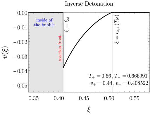
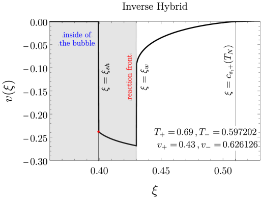
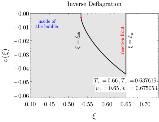
Figure 5: Fluid velocity profiles for inverse phase transitions in the plasma frame, as evaluated by solving the hydrodynamic equations with the thermodynamics derived directly from the full free energy. Due to their inverse nature, the fluid velocity for these solutions is always negative or zero in this frame. From left to right, inverse detonation, hybrid, and deflagration transitions are displayed. Further details on the computation are provided in the main text and the Appendix C.

Coupling to the SM thermal bath – In the early universe, the SUSY breaking model considered here is generally accompanied by additional spectator fields that are in thermal equilibrium with the SUSY breaking sector. To assess the impact of these additional degrees of freedom, we redefine the energy and pressure as

$$p(T)\to p(T)+\tilde{c}^{2}\tilde{a}T^{4},\quad e(T)\to e(T)+3\tilde{c}^{2}\tilde{a}T^{4}\,,$$ (9)

where we consider $\tilde{c}^{2}=1/3$ and $\tilde{a}$ controls the number of the relativistic spectator degrees of freedom (dofs), which is expected to be $\tilde{a}\sim 200\pi^{2}/30\sim 70$ considering a supersymmetric extension of the Standard Model (SM).

The presence of these fields will mostly influence the strength of the FOPT. In the limit $\tilde{a}\gg 1$, one has $\delta p/\delta e\simeq 1/3$ as expected for a gas of relativistic particles, and the generalised pseudo-trace in this limit becomes

$${}\alpha_{\vartheta}\simeq\frac{4(De-3Dp)}{3w_{+}(T_{+})}\frac{1}{1+x},\quad x=\frac{4\tilde{c}^{2}\tilde{a}T_{+}^{4}}{w_{+}(T_{+})}.$$ (10)

Thus, to a good approximation, the strength of the phase transition exhibits an inverse scaling with $\tilde{a}$, aligning with physical intuition. From explicit calculations, we find that the pseudo-trace and generalised pseudo-trace are always very close to each other in the parameter space of interest, and that the asymptotic behaviour in Eq. (10) is well established for $\tilde{a}\gtrsim 50$ leading to typical values of $\alpha_{\vartheta}\lesssim 10^{-2}$, while in the absence of spectator fields one would have $\alpha_{\vartheta}\lesssim 10^{-1}$.

In this regard, let us notice that there is in fact a fundamental difference between the strength of a standard (direct) FOPT and the case of an inverse FOPT. By referring to the definition of $\alpha_{\vartheta}$ in Eq. (8), we can see that the part containing $Dp(T_{+})$ will always contribute with a positive sign. This follows from the fact that the broken phase will necessarily have a larger pressure than the symmetric phase for the FOPT to take place and that $\delta e/\delta p\simeq 1/c_{s}^{2}$ is a positive quantity. Therefore, considering the case of negative $\alpha_{\vartheta}$, we can derive the following inequality:

$$\frac{3}{4}|\alpha_{\vartheta}|<\frac{\omega_{-}(T_{+})-\omega_{+}(T_{+})}{\omega_{+}(T_{+})}=\frac{\Delta a(T_{+})}{a_{+}(T_{+})},$$ (11)

where $a_{+}(T_{+})$ indicates the effective number of relativistic dofs in the symmetric phase at the temperature $T_{+}$, according to the parametrization of the enthalpy as $\omega/T^{4}\equiv a(T)$, and $\Delta a(T_{+})$ is the change in dofs in the broken phase at the same temperature. This relation indicates that an inverse FOPT can be very strong only when it involves a significant change in dofs between the two phases. This is a structural property of the vacua of the theory under consideration, and it should be contrasted with the case of standard FOPTs whose strength is mostly controlled by the amount of supercooling that can be achieved in the expanding universe. In particular, Eq. (11) indicates that an inverse FOPT is not necessarily stronger when it becomes more supercooled.

Conclusion and outlook – We presented a simple SUSY breaking model displaying a window of inverse FOPTs during the spontaneous breaking of the $R$–symmetry. This represents the first concrete example of a BSM model leading to an inverse FOPT in a cooling cosmology, as well as a proof of principle for the relevance of this dynamics in the early universe.

We find that the sign of the generalised pseudo-trace, $\alpha_{\vartheta}$ in Eq.(8), determines the inverseness of the transition. As a comparison, we also show that the sign of the pseudo-trace introduced in Ref. [95] offers a fair estimate for the type of the FOPT as well.

Our study motivates a broader investigation of inverse FOPTs in explicit BSM models. This includes establishing a deeper connection between the inverseness of a FOPT and its fundamental properties and symmetries, exemplified here within a model of spontaneous SUSY breaking, as well as identifying possible non–SUSY realisations of this dynamics.

As the actual hydrodynamic solution that will be realised depends on the terminal velocity of the bubble wall, our study suggests to apply and adapt the non–equilibrium techniques developed for direct FOPTs to inverse FOPTs as well.

Finally, FOPTs are powerful sources of gravitational waves that can be detected at current and forthcoming GW observatories. This work provides motivation to characterize the GW spectrum related to inverse FOPTs, and to determine to which extent this can be distinguished from the one arising during direct FOPTs.

Acknowledgments– We sincerely acknowledge Thomas Konstandin, Xander Nagels, Alberto Mariotti, David Mateos, Diego Redigolo, and Mikel Sanchez-Garitaonandia for clarifying discussions and for reading the manuscript. GB is supported by the grant CNS2023-145069 funded by MICIU/AEI/10.13039/501100011033 and by the European Union NextGenerationEU/PRTR. GB also acknowledges the support of the Spanish Agencia Estatal de Investigacion through the grant “IFT Centro de Excelencia Severo Ochoa CEX2020-001007-S”. SB is supported by the Deutsche Forschungsgemeinschaft under Germany’s Excellence Strategy - EXC 2121 Quantum universe - 390833306. MV is supported by the “Excellence of Science - EOS” - be.h project n.30820817, and by the Strategic Research Program High-Energy Physics of the Vrije Universiteit Brussel.

Appendix A Effective potential

In this appendix, we outline the computation of the one-loop and thermal corrections to the potential, as used in the main text.

One-Loop Potential.

It is well known that quantum corrections at one loop modify the shape of the scalar potential [97]. At one loop, the tree-level potential is corrected by the Coleman-Weinberg potential, given by

$$V_{\rm CW}(x)=\sum_{i=f,s}\frac{n_{i}(-1)^{F}}{64\pi^{2}}\left[M_{i}^{4}(x)\left(\log\frac{M_{i}^{2}(x)}{\Lambda^{2}}-\frac{3}{2}\right)\right]\,,$$ (12)

such that the total effective potential is

$$V_{0}(x)=V_{\rm tree}(x)+V_{\rm CW}(x)\,.$$ (13)

Here, $M_{i}(x)$ denotes the field-dependent masses of the particles in the spectrum, including the four fermionic and four scalar degrees of freedom. The sum runs over all states, with $F=1(0)$ for fermions (scalars), and $\Lambda$ is the renormalization scale, which we set to $\Lambda=m$.

Thermal corrections.

In the early universe, high temperatures and the associated thermal fluctuations modify the effective potential. These thermal effects can be incorporated by adding finite-temperature corrections to the zero-temperature potential [98, 99], leading to

$$V_{\rm eff}(T,x)=V_{0}(x)+V_{T}(x)\,.$$ (14)

Here, $V_{0}(x)$ is the one–loop effective potential derived above, while the thermal potential $V_{T}(x)$ is given by

$$V_{T}(M_{i}(x)) =\sum_{i\in B}\frac{n_{i}}{2\pi^{2}}T^{4}J_{B}\bigg{(}\frac{M_{i}^{2}(x)}{T^{2}}\bigg{)}-\sum_{i\in F}\frac{n_{i}}{2\pi^{2}}T^{4}J_{F}\bigg{(}\frac{M_{i}^{2}(x)}{T^{2}}\bigg{)},$$

$$J_{B/F}(y^{2}) =\int_{0}^{\infty}dx\ x^{2}\log\Big{[}1\mp\exp{(-\sqrt{x^{2}+y^{2}})}\Big{]}\,,$$ (15)

where the sum includes the (tree–level) massless fields in the $X$ superfield corresponding to the goldstino, the pseudomodulus, and the $R$–axion, which will give a constant, namely $x$–independent, contribution to the free energy at one loop.

The full one-loop potential, including both quantum and thermal corrections, then takes the standard form

$$V_{\rm eff}(x,T)=V_{\rm tree}(x)+\sum_{i}\left[V_{\rm CW}\big{(}M_{i}^{2}(x)\big{)}+V_{T}\big{(}M_{i}^{2}(x)\big{)}\right],$$ (16)

where we have neglected the thermal masses as they play no significant role for the FOPT under study, given that the particles contributing to the effective potential are either very massive or very light in both phases.

Appendix B Nucleation temperature

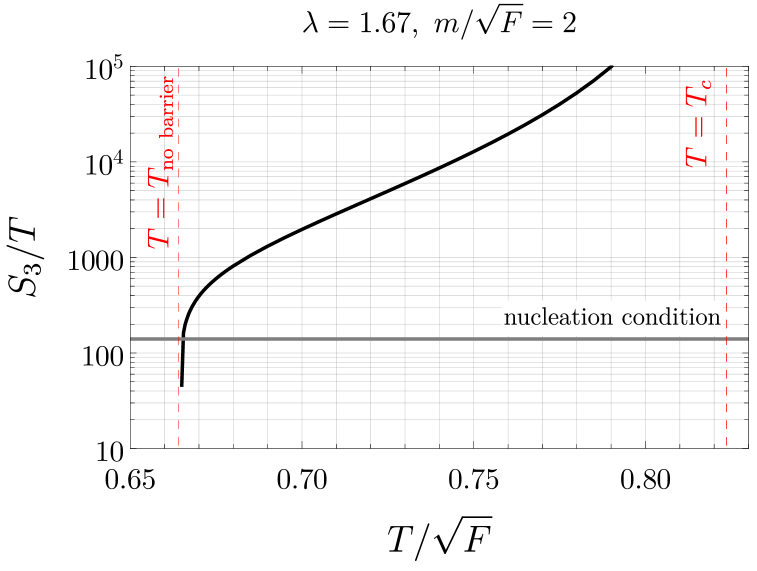
Figure 6: We present the Euclidean action as a function of temperature for the benchmark point under consideration. Assuming a nucleation criterion of $S_{3}/T\sim 140$, this corresponds to setting $\sqrt{F}\sim\text{TeV}$. As we can see, tunnelling occurs around $T_{\rm nuc}/\sqrt{F}\sim 0.665$.

In this section we study the tunnelling rate for the $R$–symmetry breaking FOPT of interest. Starting with the effective potential derived in the previous section, we can proceed to the analysis of the phase transition. FOPTs occur when the minima of the effective potential corresponding to different phases are separated by a potential barrier, so that the transition proceeds via the nucleation of bubbles. The probability of bubble nucleation per unit time and unit volume is given by [100, 101, 102]

$${}\Gamma(T)\simeq\Gamma_{3}+\Gamma_{4}=T^{4}\bigg{(}\frac{S_{3}}{2\pi T}\bigg{)}^{3/2}e^{-S_{3}(T)/T}+\frac{1}{R_{0}^{4}}\bigg{(}\frac{S_{4}}{2\pi}\bigg{)}e^{-S_{4}}\;,$$ (17)

where $S_{3}$ and $S_{4}$ are the $O(3)$ and $O(4)$ bounce actions, respectively, and $R_{0}$ is the bubble radius at nucleation. In the case of interest, the tunnelling is dominantly induced by thermal fluctuations, and we can thus neglect the $O(4)$ contribution. The probability of finding a specific point of the universe in the false vacuum at a given temperature is given by [103, 104]:

$${}P_{f}(T)=\exp[-I(T)]\;,\qquad I(T)\equiv\frac{4\pi}{3}\int^{T_{c}}_{T}\frac{dT_{1}\Gamma(T_{1})v_{w}^{3}}{T_{1}^{4}H(T_{1})}\bigg{[}\int_{T}^{T_{1}}\frac{dT_{2}}{H(T_{2})}\bigg{]}^{3}.$$ (18)

In Eq.(17), the strongest dependence on the temperature comes from $\Gamma(T)\propto\exp{(-S_{3}/T)}$, so that the quantity $I(T)$ is mostly controlled by the ratio $\Gamma\left(T\right)/H\left(T\right)^{4}$, and one can estimate that, on average, one bubble has nucleated in one Hubble volume when $\Gamma(T)\sim H(T)^{4}$. The temperature that satisfies this condition is referred to as the nucleation temperature, $T_{\rm nuc}$. The nucleation condition $\Gamma\sim H^{4}$ approximately reads

$$\frac{S_{3}}{T}\bigg{|}_{T=T_{\rm nuc}}\sim 4\log\left(\frac{T_{\rm nuc}}{H}\right)\sim 140,$$ (19)

where in the last step we have considered a FOPT occurring around $T_{\text{nuc}}\sim\ 1\,\text{TeV}$. One can additionally define the percolation temperature, $T_{\rm per}$, as the temperature when a significant fraction of space, customarily taken to be $\sim$ 34%, has been converted to the true vacuum:

$${}I(T\equiv T_{\rm per})=0.34.$$ (20)

For relatively fast FOPTs, one however has $T_{\text{per}}\simeq T_{\text{nuc}}$.

The bounce solution and the corresponding bounce action are obtained via the well-known overshoot/undershoot method to solve the equations of motion for bubble nucleation. We present the value of the ratio $S_{3}/T$ as a function of $T$ in Fig. 6 for the benchmark point with $\lambda=1.67,m/\sqrt{F}=2$ as in the main text.

Another important quantity characterising the FOPT is its duration, which is related to the radius of bubbles at collision, $R_{\star}$, by the approximate relation [105]:

$${\beta\over H}\simeq\frac{(8\pi)^{1/3}}{R_{\star}H}\;,$$ (21)

where $\beta$ is given by

$${}\beta\equiv-\frac{d}{dt}\frac{S_{3}}{T}\bigg{|}_{T=T_{\rm nuc}}=HT\frac{d}{dT}\frac{S_{3}}{T}\bigg{|}_{T=T_{\rm nuc}}.$$ (22)

Appendix C Solving the Hydrodynamic Equations for the Fluid Profiles

The conservation of the energy-momentum tensor for a relativistic fluid, given by

$$\nabla_{\mu}T^{\mu\nu}=0,$$ (23)

yields two independent hydrodynamic equations: one for energy conservation and another for momentum conservation. These equations can be rewritten in terms of the enthalpy density, $w=e+p$, as

$$\partial_{\xi}\left[w\gamma^{2}v\right] =0,$$ (24)

$$\partial_{\xi}\left[w\gamma^{2}v^{2}+p\right] =0.$$ (25)

We consider a spherically symmetric and self-similar configuration, where the fluid variables depend only on $\xi=r/t$, the similarity variable. In this variable, we can express Eqs. (24) and (25) in differential form

$$(\xi-v)\frac{\partial_{\xi}e}{w} =\frac{2v}{\xi}+[1-\gamma^{2}v(\xi-v)]\partial_{\xi}v,$$ (26)

$$(1-\xi v)\frac{\partial_{\xi}p}{w} =\gamma^{2}(\xi-v)\partial_{\xi}v.$$ (27)

To express Eq. (27) in terms of $v$ and $T$, we use the thermodynamic relation

$$\frac{\partial_{\xi}p}{w}=\frac{\partial_{\xi}T}{w}\frac{dp}{dT}=\frac{\partial_{\xi}T}{T}.$$ (28)

This leads to the temperature evolution equation

$$\frac{\partial_{\xi}T}{T}=\gamma^{2}\mu(\xi,v)\partial_{\xi}v,\qquad\mu(\xi,v)=\frac{\xi-v}{1-\xi v}\,,$$ (29)

where $\mu(\xi,v)$ is the Lorentz transformed velocity. Thus, the coupled system of hydrodynamic equations can be rewritten solely in terms of the velocity and temperature profiles, $v(\xi)$ and $T(\xi)$,

$$(\xi-v)\frac{\partial_{\xi}T}{w}\frac{de}{dT} =\frac{2v}{\xi}+[1-\gamma^{2}v(\xi-v)]\partial_{\xi}v,$$ (30)

$$\frac{\partial_{\xi}T}{T} =\gamma^{2}\mu(\xi,v)\partial_{\xi}v.$$ (31)

It is important to emphasize that the thermodynamic quantities, such as $p$ and $e$, must be evaluated in the appropriate phase depending on the region where the equation is being solved. Specifically, when computing the rarefaction wave of a detonation, the relevant phase is the newly formed one, corresponding to the true vacuum. Conversely, in the case of an inverse detonation, the quantities must be evaluated in the initial phase, corresponding to the false vacuum.

In the remainder of this section, we present the different types of expansion modes for inverse PTs within this general framework.

Inverse Deflagration

To fully specify the system of equations in Eqs. (30), we must define the initial conditions for $v(\xi)$ and $T(\xi)$. In the case of an inverse deflagration, this translates to

$$\xi_{w} =v_{+},\qquad v(\xi_{w})=\mu(v_{+},v_{-}),$$ (32)

$$T(\xi_{w}^{+}) =T_{+},\qquad T(\xi_{w}^{-})=T_{-},$$ (33)

where the $+$ phase corresponds to the false vacuum, while the $-$ phase corresponds to the true vacuum.

Additionally, we impose the condition for the formation of a shock wave, which is given by

$$\mu(\xi_{sh},v(\xi_{sh}))\xi_{sh}=c_{s,-}^{2}(T(\xi_{sh}))\,.$$ (34)

Here we emphasize that, as we are considering the full temperature dependence of the free energy of our system rather than the approximate form based for instance on the bag EoS, the speed of sound is temperature dependent and must be evaluated in the $-$ phase at the temperature corresponding to the given point in the fluid profile. An example of such a solution is shown in the right panel of Fig. 5.

These initial conditions also apply to standard detonations, provided that the pair $(v_{+},v_{-})$ satisfies the necessary condition $v_{+}>v_{-}$.

Inverse Detonations

For inverse detonations, the initial conditions across the discontinuity translate into

$$\xi_{w} =v_{-},\qquad v(\xi_{w})=\mu(v_{-},v_{+}),$$ (35)

$$T(\xi_{w}^{+}) =T_{+},\qquad T(\xi_{w}^{-})=T_{-}\,.$$ (36)

It can be checked directly that the rarefaction wave terminates at

$$\xi_{\rm end}=c_{s,+}(T(\xi_{\rm end}))\,.$$ (37)

For a standard detonation, the substitution $c_{s,+}\to c_{s,-}$ must be applied, as the rarefaction wave develops behind the reaction front, i.e., in the new phase.

These initial conditions also apply to standard deflagrations, provided that the pair $(v_{+},v_{-})$ satisfies the appropriate conditions. In this case, the shock condition in Eq. (34) must be modified by replacing $c_{s,-}$ with $c_{s,+}$, as the shock forms ahead of the reaction front in the old phase.

Before discussing the last type of solution, it is important to highlight the presence of strong solutions in Fig. 7, where the red-shaded region indicates their domain. For (inverse) detonations, the strong regime is defined by the conditions

$${}\text{Strong detonation:}\quad v_{-}<c_{s,-}(T_{-})\,,\qquad\text{Strong inverse detonation:}\quad v_{+}>c_{s,+}(T_{+})\,.$$ (38)

Similarly, for (inverse) deflagrations, we have

$${}\text{Strong deflagration:}\quad v_{-}>c_{s,-}(T_{-})\,,\qquad\text{Strong inverse deflagration:}\quad v_{+}<c_{s,+}(T_{+})\,.$$ (39)

As previously discussed in [83], strong (inverse) detonations cannot be consistently realised, while strong (inverse) deflagrations, although they may initially form due to the dynamics of the phase transition, are inherently unstable. Over time, they will decay into (inverse) hybrid solutions.

Inverse Hybrid

For inverse hybrid solutions, as in the standard case, to make the profile stable, we must connect a strong inverse deflagration to a Chapman-Jouguet inverse detonation, which is defined as a detonation with $v_{+}=c_{s,+}(T_{+})$. The initial conditions then translate into

$$v(\xi_{w}^{+}) =\mu(\xi_{w}^{+},c_{s,+}(T_{+})),\qquad v(\xi_{w}^{-})=\mu(\xi_{w}^{-},v_{-}),$$ (40)

$$T(\xi_{w}^{+}) =T_{+},\qquad T(\xi_{w}^{-})=T_{-}\,,$$ (41)

where the four input parameters required to specify the system are $(\xi_{w},v_{-},T_{+},T_{-})$.

Additionally, the shock formation condition given by Eq. (34) must be imposed, and one can verify that the rarefaction wave of the inverse detonation terminates at Eq. (37). As explained in the main text, the maximal range of wall velocities for which an inverse hybrid solution exists is given by

$$c_{s,-}^{2}<\xi_{w}<c_{s,+}\,,$$ (42)

where the lower bound arises because the slowest possible inverse hybrid is determined by the slowest possible shock.

For the case of a direct hybrid transition, a strong deflagration must instead be connected to a CJ detonation, where the latter is characterized by $v_{-}=c_{s,-}(T_{-})$. The allowed range of wall velocities in this case is

$$c_{s,-}<\xi_{w}<1\,,$$ (43)

where the upper bound is simply the speed of light, as there is no fundamental constraint on the maximum speed of the shock front.

Overlap in the hybrid corner

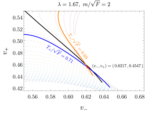
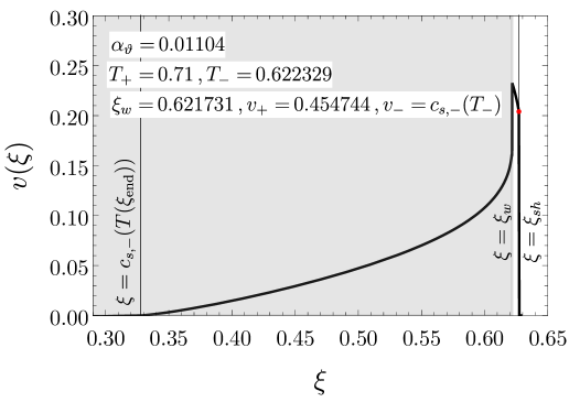
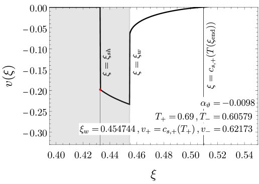
Figure 7: Overlap of direct and inverse branches in the $(v_{-},v_{+})$ plane and corresponding fluid profiles. Left panel: The $(v_{-},v_{+})$ trajectories for different values of $T_{+}$. The inverse branch is shown in orange, while the direct branch is displayed in blue. The highlighted crossing point indicates a case where both a direct and an inverse solution exist for the same $(v_{-},v_{+})$ pair. Middle panel: Fluid profile corresponding to the direct hybrid solution. Right panel: Fluid profile for the inverse hybrid solution. The shaded regions indicate the interior of the bubble. The numerical values of $\alpha_{\vartheta}$ and relevant hydrodynamic parameters are reported in each panel.

In our numerical analysis, we observe that in the hybrid transition regime, the branches in the $(v_{-}-v_{+})$ plane exhibit an overlap between direct and inverse transitions. This is particularly evident when zooming in on the hybrid region, as shown in Fig. 7 (left panel). There, we explicitly construct two distinct solutions corresponding to the same pair of values $(v_{-},v_{+})$, demonstrating the existence of overlapping branches, in the middle and right panel of Fig. 7.

This overlap arises due to the stability conditions required for hybrid solutions. Specifically, for both direct and inverse hybrids to remain stable, the fluid velocity just behind (or in front of) the wall must match the local speed of sound in the respective phase at the corresponding temperature. That is, stability demands that

$$\text{inverse hybrid:}\qquad v_{+}=c_{s,+}(T_{+}),\qquad\qquad\text{hybrid:}\qquad v_{-}=c_{s,-}(T_{-}).$$ (44)

This condition provides additional flexibility in setting $\xi_{w}=v_{-}$ for direct hybrids and $\xi_{w}=v_{+}$ for inverse hybrids, thus allowing both solutions to coexist.

Another key reason for this overlap is related to the structure of the separatrices (black solid lines) in the $(v_{-},v_{+})$ plane. Ideally, these separatrices would be given by

$$v_{-}=v_{+},\quad v_{-}v_{+}=c_{s,-}^{2},$$ (45)

but since the speed of sound varies along the branches due to temperature dependence, the boundary between the direct and inverse solutions is no longer sharply defined.

Despite their overlap in the $(v_{-},v_{+})$ plane, the two solutions can still be distinguished physically. Each branch corresponds to a different set of temperatures $(T_{+},T_{-})$, leading to a different transition strength characterized by the generalised pseudotrace, $\alpha_{\vartheta}$, which will have in fact a different sign. Thus, even though the solutions may appear degenerate in velocity space, they remain distinct due to their thermodynamic properties. The matching conditions and the sign of $\alpha_{\vartheta}$ remain robust criteria for distinguishing direct and inverse transitions.

Appendix D Inverse FOPTs in $\mu\nu$ model

In this section, we examine the emergence of inverse phase transitions in the $\mu\nu$-model [106], also referred to as the $\nu$-model in Ref. [95] and the template model in Refs. [107, 108, 109]. The $\mu\nu$-model extends the standard bag model by allowing the sound speed to deviate from the relativistic value of $1/\sqrt{3}$, while remaining constant within each phase. Explicitly, the EoS for the symmetric and broken phases is given by

$$e_{+}(T)=a_{+}T^{\nu}+\epsilon_{+}\,,\quad\qquad\ \ p_{+}(T)=c_{s,+}^{2}a_{+}T^{\nu}-\epsilon_{+}\,,$$ (46)

$$e_{-}(T)=a_{-}T^{\mu}+\epsilon_{-}\,,\quad\qquad\ \ p_{-}(T)=c_{s,-}^{2}a_{-}T^{\mu}-\epsilon_{-}\,,$$ (47)

where the constants $\nu$, $\mu$ are related to the sound speed in the symmetric and broken phases through

$$\nu=1+\frac{1}{c^{2}_{s,+}}\,,\quad\mu=1+\frac{1}{c^{2}_{s,-}}\,.$$ (48)

The symmetric phase within our SUSY model corresponds to the $+$ phase, where $\langle x\rangle=0$, and we consider $\mu>\nu$ as this mimics the thermal history of the $R$–symmetry model. In this setup, the symmetric phase is energetically favoured both at $T=0$ and $T\gg T_{c}$, while the broken phase becomes dominant at intermediate temperatures.

In this model, the velocity relations from the matching conditions take the form:

$$v_{+}v_{-} =\frac{\mu-\mu\nu-r\nu(3\alpha_{\theta}-1)(\mu-1)}{\big{(}\mu-\mu\nu+r\nu(3\alpha_{\theta}+\mu-1)\big{)}(\mu-1)}\,,$$ (49a)

$$\frac{v_{+}}{v_{-}} =\frac{(\mu-1)\big{(}\mu-\mu\nu+r\nu(3\alpha_{\theta}-1)\big{)}}{\mu-\mu\nu-r\nu(3\alpha_{\theta}+\mu-1)(\mu-1)}\,.$$ (49b)

where we define the ratio $r$ as

$$r\equiv\frac{a_{+}T^{\nu}_{+}}{a_{-}T^{\mu}_{-}}\,.$$ (50)

Additionally, the strength parameter $\alpha_{\theta}$ defined from the pseudo trace $\theta$ as

$$\theta=e-p/{c_{s,-}^{2}}\,\,,\quad\alpha_{\theta}\equiv\frac{4D\theta}{3w_{+}},$$ (51)

within the $\mu\nu$ model evaluates to:

$$\alpha_{\theta}=\frac{\nu-1}{3\nu}\left(\frac{\nu-\mu}{\nu-1}+\mu\alpha_{+}\right),\qquad\alpha_{+}\equiv\frac{\Delta\epsilon}{a_{+}T^{\nu}_{+}}=\frac{\epsilon_{+}-\epsilon_{-}}{a_{+}T^{\nu}_{+}}\,.$$ (52)

It is important to emphasize that $\alpha_{\theta}$ serves as the fundamental quantity determining the nature of the transition, and directly corresponds to the strength of the phase transition computed via the pseudo-trace.

Notably, in the case of the traditional Bag EoS, where $\mu=\nu=4$, the pseudo-trace coincides with the standard definition of the phase transition strength, $\alpha_{\theta}=\alpha_{+}$, thereby recovering the standard velocity relations.

The direct (dashed lines) and inverse (solid lines) branches are presented in Fig. 8. As shown in the figure, as soon as $\alpha_{\theta}<0$, the inverse branches emerge. This confirms that in the $\mu\nu$-model, a negative $\alpha_{\theta}$ implies an inverse phase transition. Analogously, for the Bag EoS, a negative $\alpha_{+}$ corresponds to an inverse PT. This result aligns with the characterization proposed in [83], where it was shown that within the Bag EoS, $\Delta\epsilon<0$ serves as a direct indicator of an inverse phase transition.

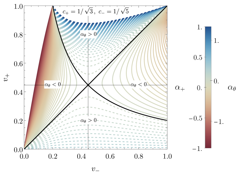
Figure 8: Dashed lines represent direct phase transitions, while solid lines correspond to inverse phase transitions. The inverse branches emerge as soon as $\alpha_{\Theta}<0$, whereas this is not necessarily the case for $\alpha_{+}$. The two strength parameters of the phase transition, $\alpha_{+}$ and $\alpha_{\Theta}$, coincide in the bag model when $\mu=\nu=4$. The color gradient illustrates the variation of $\alpha_{\theta}$, highlighting the distinct regions of direct and inverse transitions.

Appendix E Velocity of the bubble

Together with the strength, $\alpha_{\vartheta}$, the duration, $\beta^{-1}$, and the nucleation temperature, another crucial parameter for the description of the phase transition is the velocity of the bubble wall. In principle, there are two qualitatively different possibilities: 1) the bubble wall reaches a steady state, described by an (inverse) deflagration, (inverse) detonation or (inverse) hybrid or the bubble wall keeps accelerating until collision. The following study aims at clarifying which of the two is realised, following the methods presented in [110, 83, 111].

E.1 Collisionless regime computation

In principle, the possibility of runaway can be studied in the collisionless limit (see however [110]), since in this case, the wall boost factor becomes very large $\gamma_{w}\gg 1$, the pressure from the exchange of momentum originates from some particles losing their mass and inducing a kick on the wall. In the fast wall limit, no particle can escape the bubble, so we can consider only the entering species. To obtain the exchange of momentum, in the wall frame, we can apply the conservation of energy along the particle trajectory,

$${}E_{i}=\sqrt{m_{i}^{2}+p^{2}_{z,i}+p_{\perp}^{2}}\,,\qquad\frac{dE}{dz}=\bigg{(}\frac{dm_{i}^{2}}{dz}+\frac{dp_{z,i}^{2}}{dz}\bigg{)}\frac{1}{2E}=0\,,\qquad\Rightarrow\Delta p^{\rm part}_{z,i}\approx-\frac{\Delta m_{i}^{2}}{2p_{z}}\,,$$ (53)

where $\Delta m^{2}$ has to be understood as the change of mass of the particle $i$ upon crossing the wall. By conservation of momentum, the wall receives an equal and opposite kick, $\Delta p^{\rm part}_{z}=-\Delta p^{\rm wall}_{z}>0$, which accelerates it forward or backwards depending on the sign of the kick. We observe that a particle gaining mass induces a negative kick, and so resists the expansion of the wall, while a particle losing mass sucks the wall. In the model under consideration, both types of particles are present, so the competition between them will determine the sign of the collisionless pressure. To capture the pressure induced by the plasma, we need to further convolute the momentum with the incoming flux:

$$\mathcal{P}_{\rm plasma} =\int dz\partial_{z}\phi\sum_{i}g_{i}\frac{dm^{2}_{i}(\phi)}{d\phi}\int\frac{d^{3}{\bf p}}{(2\pi)^{3}2E_{i}}\,f_{i}(p,z,T)\approx\sum_{i}g_{i}\int\frac{d^{3}{\bf p}}{(2\pi)^{3}}\frac{\Delta m^{2}_{i}}{2E_{i}}f^{\rm eq}_{\rm outside}(p,T)\,.$$ (54)

where the sum is to be performed over all particles which may lose or gain a mass across the bubble wall, and $g_{i}$ is the number of dofs for each particle. By convention, a negative pressure sucks the wall while a positive one resists the expansion. The integral over the phase space is frame-independent and we compute it in the plasma frame. On the other hand, the force exerted by the vacuum energy is given by

$${}F_{\rm vacuum}\equiv\int dz\partial_{z}\phi\frac{dV^{T=0}(\phi)}{d\phi},$$ (55)

Therefore, evaluating the pressure from Eq.(54) in the limit $\gamma_{w}\to\infty$ if the following inequality is satisfied,

$${}\mathcal{P}^{\gamma_{w}\to\infty}_{\rm plasma}-F_{\rm vacuum}<0\,,$$ (56)

then the wall can in principle runaway. Numerical evaluation shows that for the inverse PT window studied in this paper, $F_{\rm bubble}>0$, implying that runaway is not possible.

E.2 Local thermal equilibrium approach

In the regime of very small velocities, one can approximate that the fluid inside the bubble wall can reach thermalisation, i.e. local thermal equilibrium [112, 108, 110]. In this case, the entropy current is conserved inside the wall as well and one can solve exactly the matching conditions. In this case, the pushing plasma effect is given by

$$\mathcal{P}_{\rm plasma}\equiv-\int dz\partial_{z}\phi\sum_{i}\frac{dm^{2}_{i}(\phi)}{d\phi}\int\frac{d^{3}{\bf p}}{(2\pi)^{3}2E_{i}}\,f_{i}(p,z,T)=\mathcal{P}_{\rm LTE}+\mathcal{P}_{\rm dissipative}\ .$$ (57)

In the LTE approach, we ignore the dissipative contributions. The approximate LTE expression becomes (when we can approximate $T_{+}\approx T_{-}$):

$${}F_{\rm vacuum}-\mathcal{P}_{\rm plasma}\approx\frac{3w_{+}}{4}\bigg{(}\frac{1}{4}(b-1)-|\alpha_{+}|\bigg{)}\ ,\quad b\equiv a_{-}/a_{+}\,,$$ (58)

where now $b>1$. We observe that the driving force fuelling the expansion now originates from the change of d.o.f. and has to overcome the resisting force from the vacuum. For the case at hand, one can observe that $b\sim 2$, which suggests that, as $|\alpha_{+}|$ is always much smaller than $1/4$, the wall can expand within the LTE approach.

Combining the results from the Collisionless and LTE approach, one can expect the wall to reach a steady state rather than run away.

References

- [1] V. A. Kuzmin, V. A. Rubakov, and M. E. Shaposhnikov Phys. Lett. B 155 (1985) 36.
- [2] M. Shaposhnikov JETP Lett. 44 (1986) 465–468.
- [3] A. E. Nelson, D. B. Kaplan, and A. G. Cohen Nucl. Phys. B 373 (1992) 453–478.
- [4] M. Carena, M. Quiros, and C. E. M. Wagner Phys. Lett. B 380 (1996) 81–91, [hep-ph/9603420].
- [5] J. M. Cline Phil. Trans. Roy. Soc. Lond. A 376 (2018), no. 2114 20170116, [arXiv:1704.08911].
- [6] A. J. Long, A. Tesi, and L.-T. Wang JHEP 10 (2017) 095, [arXiv:1703.04902].
- [7] S. Bruggisser, B. Von Harling, O. Matsedonskyi, and G. Servant JHEP 12 (2018) 099, [arXiv:1804.07314].
- [8] S. Bruggisser, B. Von Harling, O. Matsedonskyi, and G. Servant Phys. Rev. Lett. 121 (2018), no. 13 131801, [arXiv:1803.08546].
- [9] S. Bruggisser, B. von Harling, O. Matsedonskyi, and G. Servant JHEP 08 (2023) 012, [arXiv:2212.11953].
- [10] D. E. Morrissey and M. J. Ramsey-Musolf New J. Phys. 14 (2012) 125003, [arXiv:1206.2942].
- [11] A. Azatov, M. Vanvlasselaer, and W. Yin JHEP 10 (2021) 043, [arXiv:2106.14913].
- [12] P. Huang and K.-P. Xie JHEP 09 (2022) 052, [arXiv:2206.04691].
- [13] I. Baldes, S. Blasi, A. Mariotti, A. Sevrin, and K. Turbang Phys. Rev. D 104 (2021), no. 11 115029, [arXiv:2106.15602].
- [14] E. J. Chun, T. P. Dutka, T. H. Jung, X. Nagels, and M. Vanvlasselaer arXiv:2305.10759.
- [15] A. Falkowski and J. M. No JHEP 02 (2013) 034, [arXiv:1211.5615].
- [16] I. Baldes, Y. Gouttenoire, and F. Sala JHEP 04 (2021) 278, [arXiv:2007.08440].
- [17] J.-P. Hong, S. Jung, and K.-P. Xie Phys. Rev. D 102 (2020), no. 7 075028, [arXiv:2008.04430].
- [18] A. Azatov, M. Vanvlasselaer, and W. Yin JHEP 03 (2021) 288, [arXiv:2101.05721].
- [19] I. Baldes, Y. Gouttenoire, F. Sala, and G. Servant JHEP 07 (2022) 084, [arXiv:2110.13926].
- [20] P. Asadi, E. D. Kramer, E. Kuflik, G. W. Ridgway, T. R. Slatyer, and J. Smirnov Phys. Rev. D 104 (2021), no. 9 095013, [arXiv:2103.09827].
- [21] P. Lu, K. Kawana, and K.-P. Xie Phys. Rev. D 105 (2022), no. 12 123503, [arXiv:2202.03439].
- [22] I. Baldes, Y. Gouttenoire, and F. Sala SciPost Phys. 14 (2023) 033, [arXiv:2207.05096].
- [23] A. Azatov, G. Barni, S. Chakraborty, M. Vanvlasselaer, and W. Yin JHEP 10 (2022) 017, [arXiv:2207.02230].
- [24] I. Baldes, M. Dichtl, Y. Gouttenoire, and F. Sala arXiv:2306.15555.
- [25] M. Kierkla, A. Karam, and B. Swiezewska JHEP 03 (2023) 007, [arXiv:2210.07075].
- [26] G. F. Giudice, H. M. Lee, A. Pomarol, and B. Shakya arXiv:2403.03252.
- [27] A. Azatov, X. Nagels, M. Vanvlasselaer, and W. Yin JHEP 11 (2024) 129, [arXiv:2406.12554].
- [28] H. Kodama, M. Sasaki, and K. Sato Prog. Theor. Phys. 68 (1982) 1979.
- [29] K. Kawana and K.-P. Xie Phys. Lett. B 824 (2022) 136791, [arXiv:2106.00111].
- [30] T. H. Jung and T. Okui arXiv:2110.04271.
- [31] Y. Gouttenoire and T. Volansky arXiv:2305.04942.
- [32] M. Lewicki, P. Toczek, and V. Vaskonen arXiv:2305.04924.
- [33] E. Witten Phys. Rev. D30 (1984) 272–285.
- [34] C. J. Hogan Mon. Not. Roy. Astron. Soc. 218 (1986) 629–636.
- [35] A. Kosowsky and M. S. Turner Phys. Rev. D47 (1993) 4372–4391, [astro-ph/9211004].
- [36] A. Kosowsky, M. S. Turner, and R. Watkins Phys. Rev. Lett. 69 (1992) 2026–2029.
- [37] M. Kamionkowski, A. Kosowsky, and M. S. Turner Phys. Rev. D49 (1994) 2837–2851, [astro-ph/9310044].
- [38] A. Romero, K. Martinovic, T. A. Callister, H.-K. Guo, M. Martínez, M. Sakellariadou, F.-W. Yang, and Y. Zhao Phys. Rev. Lett. 126 (2021), no. 15 151301, [arXiv:2102.01714].
- [39] T. Bringmann, P. F. Depta, T. Konstandin, K. Schmidt-Hoberg, and C. Tasillo arXiv:2306.09411.
- [40] C. Caprini et al. JCAP 1604 (2016), no. 04 001, [arXiv:1512.06239].
- [41] ET Collaboration, M. Maggiore et al. JCAP 03 (2020) 050, [arXiv:1912.02622].
- [42] R. Pasechnik, M. Reichert, F. Sannino, and Z.-W. Wang JHEP 02 (2024) 159, [arXiv:2309.16755].
- [43] A. Azatov and M. Vanvlasselaer JHEP 09 (2020) 085, [arXiv:2003.10265].
- [44] M. T. Frandsen, M. Heikinheimo, M. Rosenlyst, M. E. Thing, and K. Tuominen JHEP 09 (2023) 022, [arXiv:2302.09104].
- [45] M. Reichert and Z.-W. Wang EPJ Web Conf. 274 (2022) 08003, [arXiv:2211.08877].
- [46] K. Fujikura, Y. Nakai, R. Sato, and Y. Wang JHEP 09 (2023) 053, [arXiv:2306.01305].
- [47] C. Delaunay, C. Grojean, and J. D. Wells JHEP 04 (2008) 029, [arXiv:0711.2511].
- [48] G. Kurup and M. Perelstein Phys. Rev. D 96 (2017), no. 1 015036, [arXiv:1704.03381].
- [49] B. von Harling and G. Servant JHEP 01 (2018) 159, [arXiv:1711.11554].
- [50] A. Azatov, D. Barducci, and F. Sgarlata JCAP 07 (2020) 027, [arXiv:1910.01124].
- [51] T. Ghosh, H.-K. Guo, T. Han, and H. Liu JHEP 07 (2021) 045, [arXiv:2012.09758].
- [52] M. Aoki, T. Komatsu, and H. Shibuya PTEP 2022 (2022), no. 6 063B05, [arXiv:2106.03439].
- [53] M. Badziak and I. Nalecz JHEP 02 (2023) 185, [arXiv:2212.09776].
- [54] U. Banerjee, S. Chakraborty, S. Prakash, and S. U. Rahaman arXiv:2402.02914.
- [55] L. Delle Rose, G. Panico, M. Redi, and A. Tesi JHEP 04 (2020) 025, [arXiv:1912.06139].
- [56] B. Von Harling, A. Pomarol, O. Pujolàs, and F. Rompineve JHEP 04 (2020) 195, [arXiv:1912.07587].
- [57] J. Halverson, C. Long, A. Maiti, B. Nelson, and G. Salinas JHEP 05 (2021) 154, [arXiv:2012.04071].
- [58] E. Morgante, N. Ramberg, and P. Schwaller Phys. Rev. D 107 (2023), no. 3 036010, [arXiv:2210.11821].
- [59] R. Jinno and M. Takimoto Phys. Rev. D 95 (2017), no. 1 015020, [arXiv:1604.05035].
- [60] A. Addazi, A. Marcianò, A. P. Morais, R. Pasechnik, J. a. Viana, and H. Yang JCAP 09 (2023) 026, [arXiv:2304.02399]. [Erratum: JCAP 03, E01 (2024)].
- [61] N. J. Craig arXiv:0902.1990.
- [62] N. Craig, N. Levi, A. Mariotti, and D. Redigolo JHEP 21 (2020) 184, [arXiv:2011.13949].
- [63] P. J. Steinhardt Nucl. Phys. B 190 (1981) 583–616.
- [64] Y. Hosotani Phys. Rev. D 27 (1983) 789.
- [65] U. A. Yajnik Phys. Rev. D 34 (Aug, 1986) 1237–1240.
- [66] K. Mukaida and M. Yamada Phys. Rev. D 96 (2017), no. 10 103514, [arXiv:1706.04523].
- [67] D. Canko, I. Gialamas, G. Jelic-Cizmek, A. Riotto, and N. Tetradis Eur. Phys. J. C 78 (2018), no. 4 328, [arXiv:1706.01364].
- [68] R. Jinno, T. Konstandin, H. Rubira, and J. van de Vis JCAP 12 (2021), no. 12 019, [arXiv:2108.11947].
- [69] R. Balkin, J. Serra, K. Springmann, S. Stelzl, and A. Weiler SciPost Phys. 14 (2023), no. 4 071, [arXiv:2105.13354].
- [70] P. Agrawal and M. Nee SciPost Phys. 13 (2022), no. 3 049, [arXiv:2202.11102].
- [71] S. Blasi and A. Mariotti Phys. Rev. Lett. 129 (2022), no. 26 261303, [arXiv:2203.16450].
- [72] P. Agrawal, S. Blasi, A. Mariotti, and M. Nee JHEP 06 (2024) 089, [arXiv:2312.06749].
- [73] R. Jinno, J. Kume, and M. Yamada Phys. Lett. B 849 (2024) 138465, [arXiv:2310.06901].
- [74] S. Blasi and A. Mariotti SciPost Phys. 18 (2025) 016, [arXiv:2405.08060].
- [75] S. Blasi, R. Jinno, T. Konstandin, H. Rubira, and I. Stomberg JCAP 10 (2023) 051, [arXiv:2302.06952].
- [76] R. Balkin, J. Serra, K. Springmann, S. Stelzl, and A. Weiler JHEP 06 (2022) 023, [arXiv:2106.11320].
- [77] J. Casalderrey-Solana, D. Mateos, and M. Sanchez-Garitaonandia arXiv:2210.03171.
- [78] R. Balkin, J. Serra, K. Springmann, S. Stelzl, and A. Weiler JHEP 02 (2025) 141, [arXiv:2307.14418].
- [79] M. Laine Phys. Rev. D 49 (1994) 3847–3853, [hep-ph/9309242].
- [80] H. Kurki-Suonio and M. Laine Phys. Rev. D 51 (1995) 5431–5437, [hep-ph/9501216].
- [81] M. Laine and K. Rummukainen Nucl. Phys. B Proc. Suppl. 73 (1999) 180–185, [hep-lat/9809045].
- [82] J. R. Espinosa, T. Konstandin, J. M. No, and G. Servant JCAP 1006 (2010) 028, [arXiv:1004.4187].
- [83] G. Barni, S. Blasi, and M. Vanvlasselaer JCAP 10 (2024) 042, [arXiv:2406.01596].
- [84] Y. Bea, J. Casalderrey-Solana, D. Mateos, and M. Sanchez-Garitaonandia arXiv:2406.14450.
- [85] M. A. Buen-Abad, J. H. Chang, and A. Hook Phys. Rev. D 108 (2023), no. 3 036006, [arXiv:2305.09712].
- [86] C. Caprini and J. M. No JCAP 01 (2012) 031, [arXiv:1111.1726].
- [87] J. B. Dent, B. Dutta, and M. Rai arXiv:2411.09757.
- [88] L. O’Raifeartaigh Nucl. Phys. B 96 (1975) 331–352.
- [89] A. E. Nelson and N. Seiberg Nucl. Phys. B 416 (1994) 46–62, [hep-ph/9309299].
- [90] K. A. Intriligator, N. Seiberg, and D. Shih JHEP 07 (2007) 017, [hep-th/0703281].
- [91] N. Arkani-Hamed, S. Dimopoulos, G. F. Giudice, and A. Romanino Nucl. Phys. B 709 (2005) 3–46, [hep-ph/0409232].
- [92] A. Arvanitaki, N. Craig, S. Dimopoulos, and G. Villadoro JHEP 02 (2013) 126, [arXiv:1210.0555].
- [93] N. J. Craig, P. J. Fox, and J. G. Wacker Phys. Rev. D 75 (2007) 085006, [hep-th/0611006].
- [94] A. Katz JHEP 10 (2009) 054, [arXiv:0907.3930].
- [95] F. Giese, T. Konstandin, and J. van de Vis JCAP 07 (2020), no. 07 057, [arXiv:2004.06995].
- [96] Y. Bea, M. Giliberti, D. Mateos, M. Sanchez-Garitaonandia, A. Serantes, and M. Zilhão arXiv:2412.09588.
- [97] S. Coleman and E. Weinberg Phys. Rev. D 7 (Mar, 1973) 1888–1910.
- [98] D. Curtin, P. Meade, and H. Ramani Eur. Phys. J. C78 (2018), no. 9 787, [arXiv:1612.00466].
- [99] M. Quiros, Finite temperature field theory and phase transitions, in ICTP Summer School in High-Energy Physics and Cosmology, pp. 187–259, 1, 1999. hep-ph/9901312.
- [100] S. R. Coleman Phys. Rev. D15 (1977) 2929–2936. [Erratum: Phys. Rev.D16,1248(1977)].
- [101] A. D. Linde Phys. Lett. 100B (1981) 37–40.
- [102] A. D. Linde Nucl. Phys. B216 (1983) 421. [Erratum: Nucl. Phys.B223,544(1983)].
- [103] J. Ellis, M. Lewicki, J. M. No, and V. Vaskonen JCAP 1906 (2019), no. 06 024, [arXiv:1903.09642].
- [104] A. H. Guth and S. H. H. Tye Phys. Rev. Lett. 44 (Apr, 1980) 963–963.
- [105] K. Enqvist, J. Ignatius, K. Kajantie, and K. Rummukainen Phys. Rev. D45 (1992) 3415–3428.
- [106] L. Leitao and A. Megevand Nucl. Phys. B 891 (2015) 159–199, [arXiv:1410.3875].
- [107] F. Giese, T. Konstandin, K. Schmitz, and J. van de Vis JCAP 01 (2021) 072, [arXiv:2010.09744].
- [108] W.-Y. Ai, B. Laurent, and J. van de Vis JCAP 07 (2023) 002, [arXiv:2303.10171].
- [109] M. Sanchez-Garitaonandia and J. van de Vis arXiv:2312.09964.
- [110] W.-Y. Ai, X. Nagels, and M. Vanvlasselaer JCAP 03 (2024) 037, [arXiv:2401.05911].
- [111] W.-Y. Ai, B. Laurent, and J. van de Vis arXiv:2411.13641.
- [112] W.-Y. Ai, B. Garbrecht, and C. Tamarit JCAP 03 (2022), no. 03 015, [arXiv:2109.13710].