Spectroscopic classification of non-ergodic populations
Abstract
Non-ergodicity impacts statistical inference in a diverse range of disciplines inside and outside of physics. However the concept of ergodicity is used inconsistently, and may refer to several nonequivalent notions. To help address this, we first identify and clarify the relationship between three major interpretations of ergodicity. We then introduce a method of spectral analysis of non-ergodicity which may be performed using data alone, and so may be applied in both numerical and empirical contexts. This may be used to identify, quantify, and classify non-ergodic populations within an ergodic decomposition. This is demonstrated with an application to the Kob-Andersen kinetically constrained lattice glass model.
Introduction
The extent to which inferences based on ensemble statistics may be applied to a single system over time (and vice versa) impacts a broad range of scientific topics outside of physics, with notable discussions currently taking place, for instance, on the temporal variability of climate [1, 2, 3, 4, 5, 6]; the interpretation of clinical data in medicine [7, 8, 9, 10, 11] and psychology [12, 13, 14, 15, 16]; and the validity of economic models [17, 18, 19, 20, 21]. In physics, this statistical equivalence is traditionally established as a consequence of the dynamical property of ergodicity, which received its first mathematically strict treatment in the form of metric indecomposability/transitivity by Birkhoff and von Neumann [22, 23], and has since been extended and generalized by many others [24, 25, 26, 27]. However this notion (often simply called ergodicity at the suggestion of von Neumann [28]) has been difficult to prove even for relatively simple physical systems (e.g. dynamical billiards [29, 30], the FPUT model [31, 32]). In disciplines where the dynamics may be many dimensional, complex, or unknown and empirically investigated, any such proof is often out of reach. Perhaps for this reason, ergodicity has branched into various related but nonequivalent notions. We broadly divide these into three categories we refer to as: metric indecomposability (MI), the equality of averages (EoA), and the equality of distributions (EoD). The choice of notion used is often discipline dependent; Molenaar’s [12] EoD-style notion of ergodicity has become an accepted standard in medicine and psychology [7, 8, 9, 10, 11, 13, 14, 15, 16], while a growing number of economics studies have adopted Peters’ [17] EoA notion [18, 19, 20, 21].
Metric indecomposability (MI)
Mathematics textbooks [33, 34] usually describe MI as a property of a measure preserving dynamical system , represented by a state space ; a -algebra over ; a probability measure ; and a dynamical transformation that is measure preserving, for all . As this setting can be a barrier to those unfamiliar with measure theory, we restrict our discussion of such systems to a continuous state/phase space with coordinates , a continuous time dynamics , and an ensemble density which is finite for all , and that is related to the measure by . This density is stationary under dynamical evolution by virtue of the presumptive measure preserving property. We furthermore assume all subspaces we refer to are members of -algebra .
In this deterministic context, system trajectories are confined to so-called invariant volumes, meaning subspaces that are static under dynamical evolution, . These are said to be decomposable if they may be divided into smaller (measure nonzero) invariant volumes. MI is the condition that (the support of , an invariant volume with unit measure) is not decomposable. Equivalently, any trajectory with initial state chosen randomly within will in the limit spend a proportion of its time in any volume equal to [34], and so sample the space as envisioned by Boltzmann/Maxwell [35, 36]. (A common misconception appears to be that MI ensures dynamical relaxation of a nonequilibrium density to , which instead follows from the stronger property of mixing [37].)
Analogous MI conditions apply in stochastic contexts [26, 38, 27, 39]. For instance, below we illustrate our spectral analysis method with a discrete-time Markov chain on a countably large 111For instance, in Fig. 3 there are states. but finite space, , wherein the role of indecomposable invariant volumes is played by recurrent classes of states. That is, subsets of the space within which a system in any state possesses a non-vanishing probability of reaching any other state after some finite number of time steps. In this context the MI condition takes the form of irreducibility, meaning there exists only a single recurrent class of states. (There may also exist transient states [26].) In contrast to measure preserving dynamical systems, where a stationary ensemble density is axiomatized 222Under certain conditions the existence of an invariant measure may be argued for deterministic systems with the Krylov-Bogolyubov theorem., for Markov chains (in which ensemble densities evolve as ) the existence of at least one ensemble density that is stationary, , follows from either the Perron-Frobenius theorem or Brouwer’s fixed-point theorem applied to the convex set of densities.
Equality of Averages (EoA)
Context notwithstanding, the ostensible role of the various ergodic theorems [24] is to establish the sufficiency of MI to ensure the equality of ensemble and time averages of a state function . For the above measure preserving dynamical system, this equality may be expressed
| (1) |
and applies for all (in this case integrable [28]) state functions , and almost all initial conditions . By almost all it is meant that if is chosen at random from within the indecomposable invariant volume , then EoA Eq. (1) holds with unit probability.
For an MI Markov chain, after time steps a system initially in state is distributed as , however this only converges to in the limit if the recurrent class of states is aperiodic [26] (similar to mixing for deterministic systems). Nevertheless, the time average of a state function over any trajectory is a Cesàro average whose almost sure convergence follows from the strong law of large numbers, so that in analogy to Eq. (1), MI establishes the EoA
| (2) |
for all states . For brevity, we do not state the corresponding Markov chains mathematics going forwards.
Equality of distributions (EoD)
EoD follows from the use of an indicator function , which is equal to unity for and vanishes otherwise. By setting in Eq. (1) with equal to the region of the state space in which the value of a dummy variable is less than original function , i.e. , one may pick out the portion of the trajectory and ensemble in which the state function is below this value so that
| (3) |
defining the equality of trajectory and ensemble (cumulative) distributions, and .
MI EoD EoA
While ergodic theorems show the sufficiency of MI to establish EoA for all functions, it is also possible to prove the necessity and so establish an equivalence. See for instance Proposition 4.1.3 of Ref. [34]. Thus,
However in practical circumstances, verification that EoA holds for all functions is clearly out reach, and potentially more difficult than proving MI. So instead we take EoA and EoD to be properties assigned on a function-by-function basis as for instance is the convention of Ref. [17]. Then, since for any particular function EoD is a stronger condition than EoA, the three conditions form the implicative hierarchy
As by contraposition EoA EoD MI, it is possible to formulate significance tests to rule out MI by holding either EoA or EoD as a null hypothesis. In each case, tests may be performed with the same data set (a sample of i.i.d. function values both over a trajectory and over an ensemble). However as EoD is a stronger condition, it is not unreasonable to expect EoD based tests to be typically more powerful, and it is simple to conceive of circumstances in which an EoD based test provides a significant result, while an EoA based test does not. Additionally, a number of established tests of distributional equality are non-parametric [42, 43, 44], meaning they may be performed without any assumptions made on the underlying distributions and . See for instance Ref. [45] in which EoD and thus MI was confidently ruled out for some amplitudes of a tapped granular system.
Non-ergodicity and ergodic decomposition
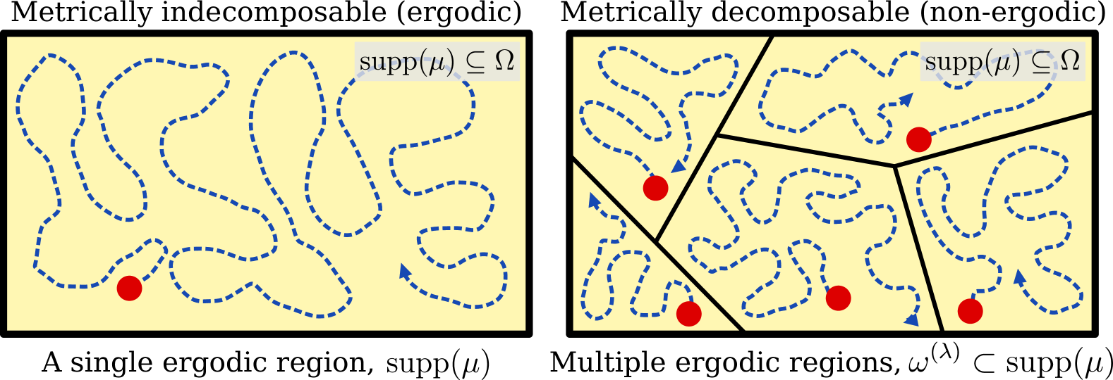
Systems that are MI wrt density are commonly referred to as being -ergodic. When this is not the case, the invariant volume may be decomposed into disjoint invariant volumes, the smallest of which are indecomposable 333See Chp. 5 of Ref. [34] for a rigorous discussion.. Denoting these , formally we write and for , though for a continuous label may take uncountable values (see e.g. Ref. [34]). Given a stationary ensemble density defined upon an indecomposable volume , so that , the dynamics is then by construction MI on this subspace, or -ergodic. Furthermore, each admits only a single unique density . To see why, suppose the dynamics did admit two distinct stationary densities and with support . As by construction the dynamics is MI wrt both, by Eq. (1) a trajectory average with a randomly chosen initial condition equates to both and . Taking results in , which holds for arbitrary , and so which we take to mean that , thus reaching the intended contradiction. As a corollary, any stationary density may be uniquely decomposed as
| (4) |
where is the proportion of ensemble members confined to invariant region . As each and , the space of stationary densities is formally a convex set with the as its extremal elements. (Of course, applied to the case of MI/-ergodicity, this argument ensures the uniqueness of .)
Ergodic and non-ergodic spectra
To describe non-ergodicity in terms of the departure from EoD (IV), first let be a measure of the statistical distance (for examples see Ref. [47]) between ensemble and trajectory distributions, and . (Going forward we suppress dependence.) Then, given a density of initial states , the overall probability density of may be expressed
| (5) |
where is a Dirac delta, and is a dummy variable taking values in the range of . We name this density the ergodicity spectrum of the system.
In contrast to a binary test of MI, construction of an ergodicity spectrum may provide information on the ergodic decomposition (4) of a non-ergodic system. To see how, note that in a non-ergodic system trajectory distributions are invariant on each ergodic region (that is, for all ), so that may be replaced with in Eq. (5). Then, using Eq. (4), the spectrum may be re-expressed as a sum over ergodic regions,
| (6) |
For an ergodic (MI) system, for all (sampled from ), and so a spectrum is a simple delta function or spectral line at . For a non-ergodic system with a countable decomposition, , key properties of a spectrum are: 1) It comprises spectral lines corresponding to each ergodic region . 2) The location of each line corresponds to the degree of deviation from EoD of -ergodic trajectories as measured by . 3) The normalization of each line corresponds to , thus indicating the prevalence of -ergodic trajectories. Note that does not necessarily map ergodic regions to distances one-to-one, so lines may overlie one another, however as demonstrated below this multiplicity can be indicative of ergodic regions that are related by a symmetry of the system/state function and so may be considered to belong to a single ergodic class. Also note that a system with a continuous state space may possess an uncountable number of ergodic regions, in which case Eq. (6) describes a continuous rather than a line spectrum.
Noise and spectral resolution in spectrum reconstruction
In practice, an ergodicity spectrum may be reconstructed by histogramming a super sample of estimates of the distributional difference , with sampled from . This introduces two types of error to be managed. Firstly, the finite size of is a source of noise in the histogram, which may be managed by adjusting the histogram bin size in the usual manner. Secondly, each estimate of is of finite accuracy, which serves to create a blurring or smearing effect on the spectrum. If for instance each estimate were a Gaussian random variable, centered on and of variance , the reconstructed spectrum would be a Gaussian blur or Weierstrass transform of the underlying spectrum (5), and in the absence of noise this would cause spectral lines to appear as such Gaussians. By analogy with astrophysical spectral analysis (see for instance Ref. [48]), would then represent the spectral resolution of the method in the sense that the underlying spectral structure in Eq. (5) should only be expected to be resolved above this lengthscale. Spectral resolution may be improved by increasing sample size (see below).
The Kolmogorov-Smirnov (KS) distance and spectrum reconstruction
Our choice of statistical distance is the KS distance, defined as the maximum vertical distance, , between two (cumulative or empirical) distributions and , and so takes values in the unit interval. We give our full justification for this choice in the SM [49] and the relevant statistical proofs in an associated paper [50]. In short though, aside from allowing for efficient calculation of unambiguous sample based estimates, properties specific to the KS distance allow us to place an analytic bound on the accuracy of such estimates, and thus also spectral resolution. Given a pair of samples and , the distance is estimated by , where and are empirical distribution functions that approximate and .
To (re)construct a spectrum from data: 1) Collect trajectory samples of size with initial configuration distributed as . 2) Collect either a single or ensemble sample(s) of size . (Figs. 2,3(a) use the latter option. See the SM [49] for a discussion of the former.) 2) From these samples calculate values of , by pairwise comparison if appropriate. 3) Create a histogram from the resulting distances.
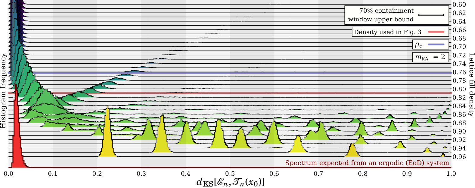
For equal sample sizes , as below, resolution is bounded by a % containment window of width not greater than , with and . Calculated values of have at least a probability to fall in window of this width centered on , and spectral structure should only be expected to be resolved above this scale. Ergodic (MI or EoD) systems appear, for large , as Kolmogorov’s PDF [51, 50] (see Figs. 2,3(a)).
Demonstration: Kob-Andersen (KA) model
The KA model [52] is a member of a class of kinetically constrained lattice glass models [53, 54], the (non-)ergodicity of which has been studied in depth by Toninelli [55]. In brief, a lattice is partially occupied by a fixed number of particles, with only one particle permitted to occupy each lattice site. The dynamics comprise each particle attempting to move with rate unity to a randomly selected neighboring site, with kinetic constrainment parameterized by integer ; each attempted move is only accepted if the particle has at most occupied neighboring sites both before and after the move.
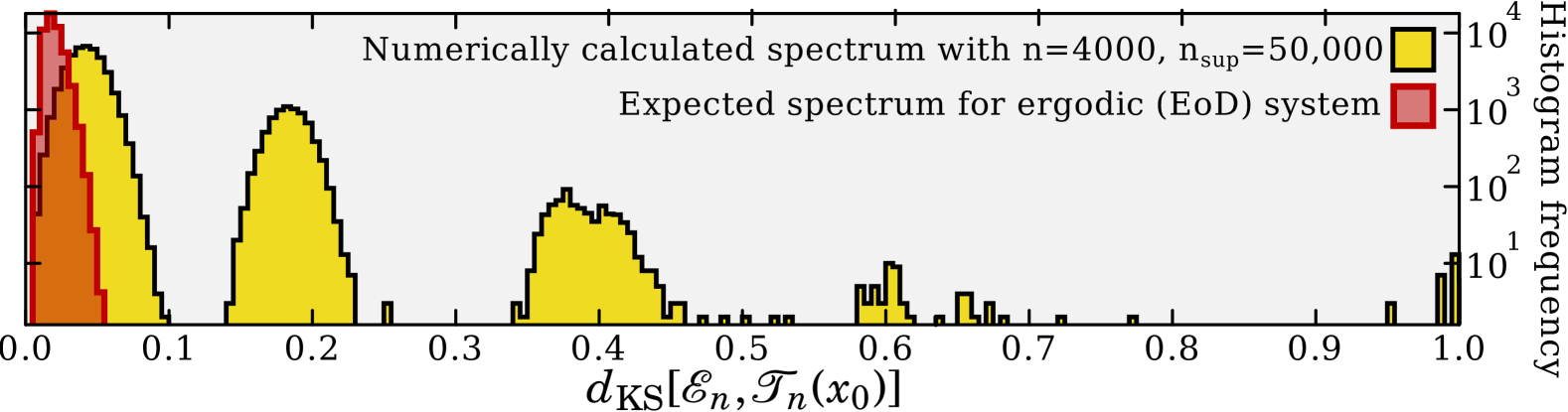
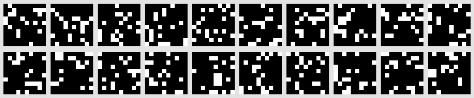
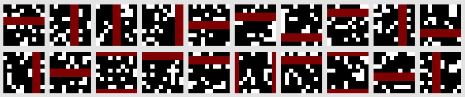
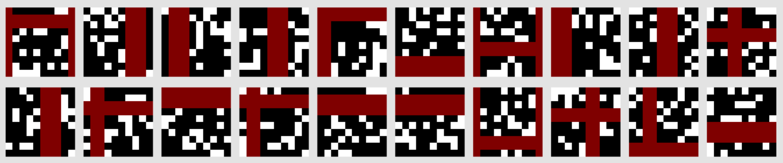
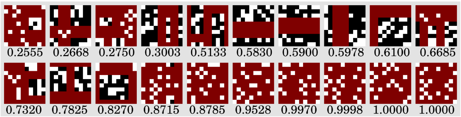
The 2d , model used in Figs. 2 and 3 is ergodic (MI) wrt the Bernoulli product measure in the thermodynamic limit . On finite lattices MI is formally broken for particle densities due to the potential for frozen structures in the configuration, the simplest of which is a adjacent pair of completely filled rows or columns. At lower densities, ergodic regions with such frozen structures are rare, and we may expect EoD and EoA to hold with high precision. Toninelli [55] describes a density dependent crossover lengthscale separating regimes where a single/many ergodic regions are sampled. For and given by the mean particle nearest neighbors, Fig. 2 displays spectra for densities surrounding the corresponding “crossover density” . The breakdown of EoD with increasing density is apparent as a shift of the bulk of the spectrum to the right is accompanied by the appearance of additional line-like features, indicating additional ergodic regions are sampled. Fig. 3 demonstrates how these line-like features correspond to classes of ergodic regions. Figs. 3(b)-3(d) show randomly selected initial configurations of trajectories producing distances in each of the first three line-like features in spectrum 3(a). The first and largest feature corresponds to no frozen structures; the second, a single adjacent pair of frozen rows/columns (a single class of ergodic regions related by rotation/translation); the third, two other types of frozen structure. We suspect due to the line shape, that this third feature may be two lines that are not resolved with the sample size used. Rare initial configurations that result in distances outside these lines feature more exotic frozen structures. Fig. 3(e) shows configurations found with a dedicated search for such cases.
Concluding remarks
After setting forth EoD as a measure of ergodicity, we have proposed a general spectroscopic method to assess and describe non-ergodicity in terms of any function of state. The spectral profile of a system has a clear and direct interpretation through Eq. (6), identifying and quantifying ergodic sub-regions and/or populations. Application of this novel method to climate and socio-economic data may help unravel invariant sub-structures in these systems.
References
- [1] L. Alexander and S. Perkins. Debate heating up over changes in climate variability. Environ. Res. Lett., 8(4):041001, (2013).
- [2] D. Olonscheck, A. Schurer, L. Lücke, and G. Hegerl. Large-scale emergence of regional changes in year-to-year temperature variability by the end of the 21st century. Nat. Commun., 12:7237, (2021).
- [3] M. Vincze, I. D. Borcia, and U. Harlander. Temperature fluctuations in a changing climate: an ensemble-based experimental approach. Sci. Rep., 7:254, (2017), arXiv:1702.07048.
- [4] G. Froyland, D. Giannakis, B. R. Lintner, M. Pike, and J. Slawinska. Spectral analysis of climate dynamics with operator-theoretic approaches. Nat. Commun., 12:6570, (2021), arXiv:2104.02902.
- [5] G. Drótos, T. Bódai, and T. Tél. Quantifying nonergodicity in nonautonomous dissipative dynamical systems: An application to climate change. Phys. Rev. E, 94:022214, (2016).
- [6] F. Flandoli and E. Tonello. Towards a defnition of climate and weather. Lect. Inst. Henri Poincaré, (2019).
- [7] A. J. Fisher, J. D. Medaglia, and B. F. Jeronimus. Lack of group-to-individual generalizability is a threat to human subjects research. Proc. Natl. Acad. Sci. U.S.A., 115(27):E6106–E6115, (2018).
- [8] J. K. Adolf and E. I. Fried. Ergodicity is sufficient but not necessary for group-to-individual generalizability. Proc. Natl. Acad. Sci. U.S.A., 116(14):6540–6541, (2019).
- [9] J. D. Medaglia, B. F. Jeronimus, and A. J. Fisher. Reply to Adolf and Fried: Conditional equivalence and imperatives for person-level science. Proc. Natl. Acad. Sci. U.S.A., 116(14):6542–6543, (2019).
- [10] M. Beil, S. Sviri, H. Flaatten, D. W. De Lange, C. Jung, W. Szczeklik, S. Leaver, A. Rhodes, B. Guidet, and P. V. van Heerden. On predictions in critical care: The individual prognostication fallacy in elderly patients. J. Crit. Care, 61:34–38, (2021).
- [11] M. Zuidersma, H. Riese, E. Snippe, S. H. Booij, M. Wichers, and E. H. Bos. Single-subject research in psychiatry: Facts and fictions. Front. Psychiatry, 11, (2020).
- [12] P. C. M. Molenaar. A manifesto on psychology as idiographic science: Bringing the person back into scientific psychology, this time forever. Meas.: Interdiscip. Res. Perspect., 2(4):201–218, (2004).
- [13] P. C. Molenaar and C. G. Campbell. The new person-specific paradigm in psychology. Curr. Dir. Psychol. Sci., 18(2):112–117, (2009).
- [14] P. C. M. Molenaar. Consequences of the ergodic theorems for classical test theory, factor analysis, and the analysis of developmental processes. In Handbook of Cognitive Aging: Interdisciplinary Perspectives. SAGE Publications Inc., (2008).
- [15] M. C. Voelkle, A. Brose, F. Schmiedek, and U. Lindenberger. Toward a unified framework for the study of between-person and within-person structures: Building a bridge between two research paradigms. Multivar. Behav. Res., 49(3):193–213, (2014).
- [16] A. G. C. Wright and W. C. Woods. Personalized models of psychopathology. Annu. Rev. Clin. Psychol., 7;16:49–74, (2019).
- [17] O. Peters. The ergodicity problem in economics. Nat. Phys., 15:1216 – 1221, (2019).
- [18] A. Vanhoyweghen, B. Verbeken, C. Macharis, and V. Ginis. The influence of ergodicity on risk affinity of timed and non-timed respondents. Sci. Rep., 12:3744, (2022).
- [19] V. Stojkoski, P. Jolakoski, A. Pal, T. Sandev, L. Kocarev, and R. Metzler. Income inequality and mobility in geometric brownian motion with stochastic resetting: theoretical results and empirical evidence of non-ergodicity. Philos. Trans. R. Soc. A, 380:20210157, (2022), arXiv:1509.03459.
- [20] A. Vanhoyweghen and V. Ginis. Human decision-making in a non-ergodic additive environment. Proc. R. Soc. Lond. A, 479:20230544, (2023).
- [21] O. Peters and M. Gell-Mann. Evaluating gambles using dynamics. Chaos, 26(2):023103, (2016), arXiv:1405.0585.
- [22] G. D. Birkhoff. Proof of the ergodic theorem. Proc. Natl. Acad. Sci. U.S.A., 17(12):656–660, (1931).
- [23] J. v. Neumann. Proof of the quasi-ergodic hypothesis. Proc. Natl. Acad. Sci. U.S.A., 18(1):70–82, (1932).
- [24] O. Kallenberg. Foundations of Modern Probability. Probability and Its Applications. Springer New York, NY, (2006).
- [25] D. Çömez. Modern Ergodic Theory: From a Physics Hypothesis to a Mathematical Theory with Transformative Interdisciplinary Impact. Springer International Publishing, Cham, (2019).
- [26] R. G. Gallager. Stochastic Processes: Theory for Applications. Cambridge University Press, Cambridge, (2013).
- [27] R. Khasminskii and G. Milstein. Stochastic Stability of Differential Equations. Springer, Berlin, Heidelberg, (2011).
- [28] C. C. Moore. Ergodic theorem, ergodic theory, and statistical mechanics. Proc. Natl. Acad. Sci. U.S.A., 112(7):1907–1911, (2015).
- [29] N. Simányi. Further Developments of Sinai’s Ideas: The Boltzmann–Sinai Hypothesis. In The Abel Prize 2013-2017, H. Holden and R. Piene (eds). Springer International Publishing, Cham, (2019), arXiv:1512.08272.
- [30] Diffusion in the Lorentz gas. Commun. Theor. Phys., 62(4):521, (2014), arXiv:1402.7010.
- [31] G. Benettin, H. Christodoulidi, and A. Ponno. The Fermi-Pasta-Ulam Problem and Its Underlying Integrable Dynamics. J. Stat. Phys., 152(2):195–212, (2013).
- [32] G. Benettin and A. Ponno. FPU Model and Toda Model: A Survey, a View. In From Kinetic Theory to Turbulence Modeling, P. Barbante, F. D. Belgiorno, S. Lorenzani, and L. Valdettaro (eds). Springer, Singapore, (2023).
- [33] P. Walters. An Introduction to Ergodic Theory. Springer New York, NY, (2000).
- [34] M. Viana and K. Oliveira. Foundations of Ergodic Theory. Cambridge University Press, Cambridge, (2016).
- [35] G. Gallavotti. Ergodicity: a historical perspective. Equilibrium and Nonequilibrium. Eur. Phys. J. H, 41(3), (2016), arXiv:1604.04239.
- [36] P. Ehrenfest and T. Ehrenfest. The Conceptual Foundations of the Statistical Approach in Mechanics. Dover, New York, (2015).
- [37] G. Benettin, R. Livi, and G. Parisi. Ergodicity: How Can It Be Broken? Volume 885, In Lecture Notes in Physics, A. Vulpiani, F. Cecconi, M. Cencini, A. Puglisi, and D. Vergni (eds). Springer, Berlin, Heidelberg, (2014).
- [38] R. M. Gray. Probability, Random Processes, and Ergodic Properties. Springer, New York, (2009).
- [39] M. Hairer. Ergodic theory for Stochastic PDEs. LMS-EPSRC Short Course on Stochastic Partial Differential Equations at Imperial College London, (2008).
- [40] For instance, in Fig. 3 there are states.
- [41] Under certain conditions the existence of an invariant measure may be argued for deterministic systems with the Krylov-Bogolyubov theorem.
- [42] W. Feller. On the Kolmogorov-Smirnov Limit Theorems for Empirical Distributions. Ann. Math. Stat., 19(2):177 – 189, (1948).
- [43] A. N. Pettitt. A two-sample anderson-darling rank statistic. Biometrika, 63(1):161–168, (1976).
- [44] T. W. Anderson. On the Distribution of the Two-Sample Cramer-von Mises Criterion. Ann. Math. Stat., 33(3):1148 – 1159, (1962).
- [45] F. Paillusson and D. Frenkel. Probing Ergodicity in Granular Matter. Phys. Rev. Lett., 109(20):208001, (2012), arXiv:1210.5407.
- [46] See Chp. 5 of Ref. [34] for a rigorous discussion.
- [47] A. L. Gibbs and F. E. Su. On Choosing and Bounding Probability Metrics. Interdisciplinary Science Reviews, 70(3):419–435, (2002), arXiv:math/0209021.
- [48] M. Ackermann et al. The Fermi Large Area Telescope on Orbit: Event Classification, Instrument Response Functions, and Calibration. Astrophys. J., 203(1):4, (2012), arXiv:1206.1896.
- [49] N. G. Underwood and F. Paillusson. Supplementary material.
- [50] N. G. Underwood and F. Paillusson. One and two sample Dvoretzky-Kiefer-Wolfowitz-Massart type inequalities for differing underlying distributions. (2024), arXiv:2409.18087.
- [51] A. Kolmogorov. Sulla determinazione empirica di una legge di distribuzione. G. Ist. Ital. Attuari, 4:83–91, (1933). Note: A number of early papers on this subject contain a typo in Kolmogorov’s distribution. See for instance [50] for a corrected version.
- [52] W. Kob and H. C. Andersen. Kinetic lattice-gas model of cage effects in high-density liquids and a test of mode-coupling theory of the ideal-glass transition. Phys. Rev. E, 48:4364–4377, (1993).
- [53] F. Ritort and P. Sollich. Glassy dynamics of kinetically constrained models. Adv. Phys., 52(4):219–342, (2003), arXiv:cond-mat/0210382.
- [54] J. P. Garrahan, P. Sollich, and C. Toninelli. Kinetically constrained models. In Dynamical Heterogeneities in Glasses, Colloids, and Granular Media, L. Berthier, G. Biroli, J.-P. Bouchaud, L. Cipelletti, and W. van Saarloos (eds). Oxford University Press, Oxford, (2011), arXiv:1009.6113.
- [55] C. Toninelli, G. Biroli, and D. S. Fisher. Cooperative Behavior of Kinetically Constrained Lattice Gas Models of Glassy Dynamics. J. Stat. Phys., 120(1-2):167–238, (2005), arXiv:cond-mat/0410647.