Topology of the simplest gene switch

Abstract

Complex gene regulatory networks often display emergent simple behavior. Sometimes this simplicity can be traced to a nearly equivalent energy landscape, but not always. Here we show how topological theory for stochastic and biochemical networks can predict phase transitions between dynamical regimes, where the simplest landscape paradigm fails. We demonstrate the utility of this topological approach for a simple gene network, revealing a new oscillatory regime in addition to previously recognized bistable and monostable phases. We show how local winding numbers predict the steady-state locations in the bistable and monostable phases, and a flux analysis predicts the respective strengths of steady-state peaks.

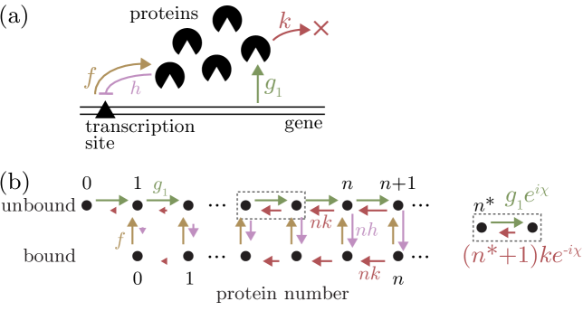
Figure 1: Self-repressing gene network. (a) A gene generates proteins with rate $g_{1}$. Each protein can degrade with rate $k$ or bind to a transcription site with rate $h$. If bound, it represses protein generation. Bound protein can unbind with rate $f$. (b) Self-repressing gene network forms a ladder given by the number of proteins $n$ and the bound vs. unbound state of the transcription factor. Right inset: to compute global spectral winding, we multiply transitions between $(n^{*},1)$ and $(n^{*}+1,1)$ states by phase factors $e^{\pm i\chi}$.

Introduction.—Gene regulatory networks often seem to resemble a giant hairball of unstructured, heterogeneous, coupled, ultimately stochastic, biochemical reactions [1] characterized by numerous, often poorly known, kinetic parameters [2]. This complexity has evolved so that organisms can cope with a variety of ever-changing environmental challenges. Nevertheless, simple stable collective behaviors often emerge from this complexity. The many stable patterns of gene expression found in different cells are often described as comprising a landscape [3]. Abstract, simplified models of stochastic gene networks have been shown to possess attractor landscapes like those of minimally frustrated Hopfield models [4, 5]. Tripathai, Kessler and Levine have recently analyzed the stability of some specific realistic gene networks to variation of parameters, concluding these networks, in fact, are minimally frustrated [6].

The quasi-equilibrium landscape picture does not exhaust all the observed regularities of gene regulation, however. The nonequilibrium character of controlled protein synthesis allows for oscillations [7] and indeed chaos [8, 9]. Such behaviors may be captured through the introduction of gauge fields to the usual reversible dynamics on the gradient of an energy envisioned in landscape theory [10, 11, 12]. Owing to these emergent gauge fields it is natural to inquire whether topology can give insights into the regularities of gene regulation.

Topology has been found to provide a theoretical prescription for the dimensional reduction of large systems to a lower-dimensional behavior [13, 14]. Topological considerations suggest that steady-state response can emerge on the edge of the state space. Crucially, such edge responses, whether as currents or localized states, are robust to random perturbations of the model, an essential element of biological robustness. Topological ideas entered physics in quantum systems [15, 16] but topological thinking has since been developed for other systems including mechanical lattices [17, 18, 19], photonic crystals [20, 21] and soft matter systems [22, 23, 24].

Topological tools have recently entered biological physics [25, 26, 27, 28, 29, 30] to describe the circadian rhythm [31], microtubule growth [28], and chemotaxis adaptation [25, 26]. Both the existing biological and physical models describe uniform lattices as their state space [25, 26, 27, 28, 29, 30, 14]. The transition network, however, is not uniform in stochastic models of gene networks. In this paper, we develop topological tools for biological networks with heterogeneous transition rates within a lattice configuration and use them to describe the simplest self-repressing or self-activating gene switch [32, 33, 34]. This network despite its simplicity can exhibit multiple steady states or oscillations. We will show local winding numbers can predict the position of the steady-states of this model both in the bistable and monostable phases and use flux analysis to predict the respective heights of steady-state peaks.

This simplest gene switch which is turned on or off by a monomeric transcription factor is remarkable in that it’s deterministic limit suggests that it should not display multistable behavior at all. Nevertheless, the exact solution does display multiple patterns of expression [32, 33]. The complexity of the simplest switch’s behavior comes from near extinction events that occur when the transcription factor number vears on vanishing. This unexpected complexity indeed comes from dynamics near the edge of the state space since copy number cannot be negative [35]. In principle all gene networks have state space with such edges where proteins become extinct at least briefly, so the topological edge features paramount in the simplest gene switch may also manifest themselves in other more realistic situations.

Global spectral winding predicts three phases in the gene switch.— Here, we introduce an invariant that predicts different dynamical regimes in a biochemical network. We start by analyzing the single transcription factor gene switch [32, 33], shown in Fig. 1(a). This is the simplest possible switch. In this system, a gene generates proteins with a constant rate $g_{1}$, while the protein acts as its own repressive transcription factor: it binds to the gene with rate $h$ and represses protein generation. The transcription factor can unbind with rate $f$, thus restoring generation. Each protein degrades with rate $k$.

This system thus forms a state space described by a vector $p_{ns}$, where $n\in\mathbb{R}_{+}^{0}$ is the number of proteins in the cell, and $s=0$ and $1$ are the off and on states of the gene, which correspond to the DNA being bound or free of bound transcription factor (see Fig. 1(b)). This probability vector is governed by the master equation $\partial_{t}p_{ns}=\sum_{mq}\mathcal{W}_{ns,mq}p_{mq}$, where the transition matrix $\mathcal{W}$ specifies the following rates: generation in on state $\mathcal{W}_{(n+1)1,n1}=g_{1}$, degradation $\mathcal{W}_{ns,(n+1)s}=(n+1)k$, binding $\mathcal{W}_{n0,(n+1)1}=(n+1)h$, and unbinding $\mathcal{W}_{(n+1)1,n0}=f$. To conserve probability, diagonal terms of the transition matrix $\mathcal{W}$ balance the sum of the outgoing transitions. The site dependence of the degradation and binding rates makes this network in state space nonuniform and thus require tools beyond those used in the usual quantum context.

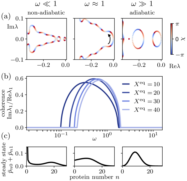
Figure 2: Global spectral winding predicts three distinct phases in self-repressing gene network. (a) Spectrum of the gene network as a function of $\chi$ shows spectral winding in three regimes of adiabaticity $\omega=f/k$, represented by $\omega=0.1$, $1$ and $5$. (b) Coherence as a function of adiabaticity $\omega$ indicates an oscillating phase at intermediate $\omega\approx 1$. (c) Steady state has two peaks in the non-adiabatic phase, spreads over the network in the oscillating phase, and has a single peak in the adiabatic phase. Coherence is shown for $X^{\mathrm{ad}}=g_{1}/2k=20$ and a range of $X^{\mathrm{eq}}=f/h$. Panels (a) and (c) use $X^{\mathrm{ad}}=X^{\mathrm{eq}}=10$.

To analyze topological properties of the gene network, we introduce a spectral winding based on threading a flux through the center of the network, a method which has been useful in studying disordered systems [36]. Practically, this entails allowing one rate of the gene network to take on a complex value whose phase $\chi$ can be swept from $-\pi$ to $\pi$, as illustrated in Fig. 1(b). Note that this flux could have been inserted on any rate (or spread across several rates) without changing any of the physics if we set $\chi=0$. Introducing $\chi$ allows us to count and envision possible cyclic paths through the state space. While the spectrum of the original transition matrix $\mathcal{W}$ is given by gray in Fig. 2(a), we see that sweeping the phase $\chi$ from $-\pi$ to $\pi$ produces a continuous change in the spectrum that forms loops, where the color denotes the spectrum calculated at a different value of $\chi$.

Notably, the loops formed appear qualitatively different for different values of the adiabaticity parameter $\omega=f/k$, which indicates speed of the binding and unbinding events compared to the generation and degradation of the protein. Note that the network also depends on two additional parameters $X^{\mathrm{ad}}=(g_{0}+g_{1})/2k$ and $X^{\mathrm{eq}}=f/h$, which we keep fixed for now. Both when $\omega\ll 1$ and when $\omega\gg 1$, small loops appear near the steady state that are composed of only two states that fold back on themselves. The next two states away from the steady state form another separate loop. In contrast, at an intermediate adiabaticity regime where $\omega\approx 1$, all the states connect to form a continuous large loop. These differences in loop size point to distinct physics, since stochastic transitions between only two states always have zero oscillatory coherence [37] in contrast to when multiple states participate.

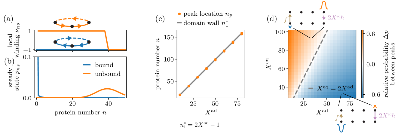
Figure 3: In the non-adiabatic phase, local winding of bound and unbound chains individually predict two peaks. (a) Local winding number is tracked along the bound (blue) and unbound (orange) chains. It is computed under periodic boundary conditions, as illustrated in two cartoons. (b) Steady state peaks in the bound and unbound chains are located at an edge and a domain wall, respectively, predicted by local winding numbers. (c) Observed peak location in the unbound states $n_{p}$ (orange dots) coincides with the predicted location of the domain wall $n^{*}_{1}$ (gray line) for a range of parameter values. (d) Relative probability between peaks $\Delta p=\sum_{n}p_{n1}-p_{n0}$ for a range of parameters $X^{\mathrm{ad}}$ and $X^{\mathrm{eq}}$. Two peaks are equal when $X^{\mathrm{eq}}=2X^{\mathrm{ad}}$. Insets: when $X^{\mathrm{eq}}>2X^{\mathrm{ad}}$, right peak is larger than left peak such that upward and downward fluxes are balanced. Similarly, right peak is smaller than left when $X^{\mathrm{eq}}<2X^{\mathrm{ad}}$. We use $X^{\mathrm{eq}}=X^{\mathrm{ad}}=20$ and $\omega=0.01$ for plots.

To test if indeed we obtain regimes with different oscillatory features, we analyze the coherence of the system. To do this, we calculate the ratio of the imaginary and real parts of the first non-trivial eigenvalue of the transition matrix $\mathcal{W}$, $\mathcal{R}=\imaginary\lambda_{1}/\real\lambda_{1}$. This expression gives the number of coherent oscillations weighted by their lifetime [37]. Indeed, we find that oscillations emerge at $\omega\approx 1$ as indicated by a non-zero coherence in Fig. 2(b), for several values of parameter $X^{\mathrm{eq}}$. These oscillations were not noticed in previous studies of this gene network [32, 33], and were only revealed upon analysis of this global winding. Instead, the previous studies described only a regime of bistability for $\omega\ll 1$ and of monostability for $\omega\gg 1$, as we can see in plots of the steady state in Fig. 2(c). While the steady state of $\omega\approx 1$ appears flat and featureless, we see this is nevertheless consistent with the system cycling across the whole network in this explicitly non-equilibrium regime.

Crucially, as we go between the small and large loop regimes, the system goes through a non-reciprocal phase transition that is characterized by a pitchfork bifurcation of the eigenvalues of the complex master equation [38]. Specifically, the two eigenvalues closest to the steady state coalesce to form an exceptional point and then split into a pair of complex-conjugated eigenvalues (see SM for details). This marks a transition between a chiral and a stationary phase [39], which has also been observed in other platforms, such as active matter [39] or optical quantum gases [40].

The global winding number [29]

$$\nu=\sum_{\varepsilon=\pm 0}\frac{1}{2\pi i}\int\limits_{0}^{2\pi}d\chi\partial_{\chi}\log\det\mathcal{W}(\chi+i\varepsilon).$$ (1)

turns out to be $+1$ for all three regimes. When the network ends in a sink, i.e. extinction in the regime of death with strictly no regeneration, however the winding number becomes 0. In this paper, we will focus on ergodic networks that do regenerate, albeit at a small rate.

In the non-adiabatic phase, local winding number predicts bistability and location of steady state peaks.—While the global spectral winding can distinguish between different dynamical regimes and identifies the phase transitions, it would be useful to predict specific quantities of interest within each phase, such as the location of the steady-state peak and the relative heights of different peaks. Here, we introduce a local winding number for this purpose. The presence of local winding numbers in a single one-dimensional chain can predict the accumulation of probability density at the system edge, also known as the non-Hermitian skin effect [41, 42, 29, 43]. However, these winding numbers are usually calculated under periodic boundary conditions [29, 43]. Here, the absence of translation symmetry in transcription factor number in many networks including ours, renders this approach inapplicable.

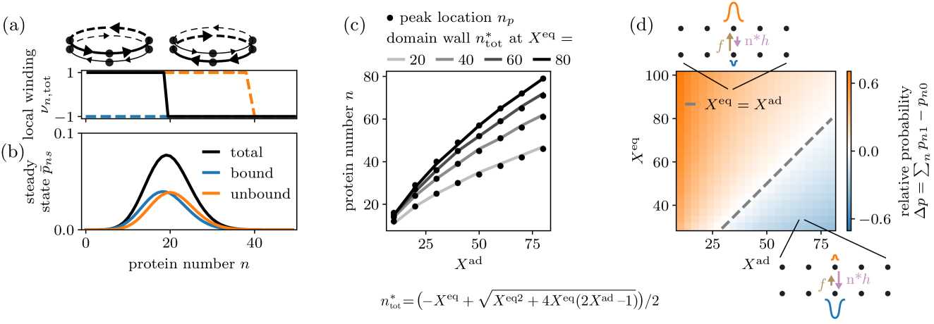
Figure 4: In the adiabatic phase, combined local winding determines domain wall and peak location. (a) Local winding number is tracked along two averaged chains (black). Cartoons illustrate two networks with periodic boundary conditions, where the unbound (resp. bound) chain dominates the net direction of winding. (b) Steady state peak in the total probability (black) is determined by the domain wall in the local winding number. (c) Observed peak location $n_{p}$ (black dots) coincides with the predicted location of the domain wall $n^{*}_{\mathrm{tot}}$ (lines of shades of gray) for a range of parameter values. (d) Relative probability between unbound and bound chains $\Delta p=\sum_{n}p_{n1}-p_{n0}$ for a range of parameters $X^{\mathrm{ad}}$ and $X^{\mathrm{eq}}$. Probabilities in two chains are equal when $X^{\mathrm{eq}}=X^{\mathrm{ad}}$. Insets: when $X^{\mathrm{eq}}>X^{\mathrm{ad}}$, unbound probability is larger than the bound such that upward and downward fluxes are balanced. Similarly, unbound probability is smaller than the bound when $X^{\mathrm{eq}}<X^{\mathrm{ad}}$. We use $X^{\mathrm{eq}}=X^{\mathrm{ad}}=20$ and $\omega=10$ for plots.

To address the lack of translation symmetry where network parameters are changing as we move along protein number $n$, we develop a local winding number that is evaluated at each index $n$ of the network. In the non-adiabatic phase $\omega\ll 1$, slow transitions between the bound and unbound chains allow the gene switch to be considered as two separate chains. We can thus define a local winding for the upper and lower (bound and unbound respectively) chains separately. For each chain, we choose a unit cell that consists of the $n$-th state of the chain together with transitions connecting it to the right neighbor. Repeating this unit cell many times leads to new periodic boundaries such that the transition matrix of the bound chain becomes $\mathcal{W}^{\mathrm{n0}}(\chi)=(n+1)k(e^{-i\chi}-1)$, and that of the unbound chain becomes $\mathcal{W}^{\mathrm{n1}}(\chi)=g_{1}(e^{i\chi}-1)+(n+1)k(e^{-i\chi}-1)$.

We compute the local winding in both bound and unbound chains by plugging these transition matrices in Eq. (1), to show in Fig. 3(a) how they change with the protein number $n$ along the network. In the bound chain, the local winding is always $\nu_{\mathrm{n0}}=-1$ along the entire chain, suggesting a polarization to the left that leads to the steady state localized on the left edge at $n^{*}_{0}=0$ (blue in Fig. 3(b)). In the unbound chain, the local winding number switches from $\nu_{\mathrm{n1}}=+1$ to $\nu_{\mathrm{n1}}=-1$ at the protein number $n^{*}_{1}=g_{1}/k-1=2X^{\mathrm{ad}}-1$, which is where the forward and backward transitions become equal to each other. This signals a domain wall at $n^{*}_{1}$, where we expect an edge state. Indeed, we find the steady state peak at this domain wall; see the orange line in Fig. 3(b) for $X^{\mathrm{eq}}=X^{\mathrm{ad}}=20$. We verify this analytical prediction by comparing it to the numerical solution of the steady state peak across a range of system parameters $X^{\mathrm{ad}}$ and $X^{\mathrm{eq}}$, to find that they match well (see Fig. 3(c)).

We can further predict which of the two peaks, bound or unbound, will be larger. Here, we use a principle of flux balance similar to Kirchhoff’s laws for electrical circuits. This principle states that the total upward flux in the gene network must be equal to the total downward flux such that $\sum_{n}J_{(n+1)1,n0}=0$. Here, the probability flux along a transition between $i$-th and $j$-th state is defined as $J_{ji}=\mathcal{W}_{ji}p_{i}-\mathcal{W}_{ij}p_{j}$. Since at the steady state there are two narrow peaks in the non-adiabatic phase, we can use flux balance to determine the relative sizes of the peaks. The bound peak at $n=0$ with the total probability $p_{0}$ causes an upwards flux $J_{\uparrow}\approx fp_{0}$. At the same time, the unbound peak at $n\approx 2X^{\mathrm{ad}}$ with the total probability $p_{1}$ causes a downwards flux $J_{\downarrow}\approx 2X^{\mathrm{ad}}hp_{1}$. Since $J_{\uparrow}=J_{\downarrow}$, the two peaks are equal when $2X^{\mathrm{ad}}=f/h=X^{\mathrm{eq}}$ (dashed line in Fig. 3(d)). We predict that the unbound peak is larger than the bound peak when $X^{\mathrm{eq}}>2X^{\mathrm{ad}}$ and vice versa, which we also confirm numerically in Fig. 3(d).

In the adiabatic phase, local winding number predicts mono-stability and location of steady-state.—In the adiabatic phase $\omega\gg 1$, fast transitions between the bound and unbound chains cause the system to average over these states, similar to the Shea-Ackers model [44]. Due to this averaging, we define a combined local winding number for coupled bound and unbound states. This local winding would then predict the steady state of the full gene network.

To define this invariant, we choose a unit cell that consists of the $n$-th state in the bound chain and the $(n+1)$-th state in the unbound chain, together with transitions between these states as well as transitions to and from their right neighbors (see SM for details). Imposing periodic boundary conditions on this unit cell, we obtain the combined local periodic network and compute the corresponding local winding number using Eq. (1). Plotting the combined local winding as a function of the protein number $n$ in Fig. 4(a), we observe that it changes sign over a domain wall, when the winding of the bound chain starts dominating over the unbound chain, as illustrated in cartoons above the plot.

The domain wall in the combined winding number determines the location of the steady state peak, as we illustrate in Fig. 4(b). To analytically derive the domain wall location, we use the fact that the sign of the winding number equals to the sign of the probability flux along the periodic network [29]. Therefore, the local winding number changes sign where probability flux vanishes. We use this to derive that the domain wall (details in the SM) is located at $n^{*}_{\mathrm{tot}}=\left(-X^{\mathrm{eq}}+\sqrt{(X^{\mathrm{eq}})^{2}+4X^{\mathrm{eq}}(2X^{\mathrm{ad}}-1)}\right)/2$. To confirm this prediction, we verify in Fig. 4(c) that the domain wall determines the peak location for a range of parameters $X^{\mathrm{ad}}$ and $X^{\mathrm{eq}}$. We note that when defining the global winding number, we used the same value of protein number $n^{*}=n^{*}_{\mathrm{tot}}$ to introduce the complex phase factor.

Similar to what was done for the non-adiabatic phase, we can use flux balance to predict the probability distribution between bound and unbound chains. With both bound and unbound peaks located at $n=n^{*}_{\mathrm{tot}}$, the up and down fluxes are $J_{\uparrow}\approx fp_{0}$ and $J_{\downarrow}\approx n^{*}_{\mathrm{tot}}hp_{1}$. Probabilities are equally distributed when $n^{*}_{\mathrm{tot}}=f/h=X^{\mathrm{eq}}$, which is true when $X^{\mathrm{ad}}\approx X^{\mathrm{eq}}$ (dashed line in Fig. 3(d)). We numerically confirm this prediction in Fig. 3(d).

Conclusion.—We have developed topological methods for stochastic systems that break translation symmetry and demonstrate them on the simplest gene network. We see there are three different phases even for this simple network, and several crucial properties of its steady state, such as peak location and relative heights, can be understood topologically. These results pave the way for future explorations using the lens of topology. For instance, relaxation times are predicted to scale differently due to topology [29], which would have biological consequences. Another interesting regime is when the global winding number goes to zero, i.e. the non-ergodic limit [43] which applies where the transcription factor can go extinct without the possibility of regeneration.

More broadly, our methods can be generalized to other biological networks with similar underlying structure. This includes the case of dimer binding instead of monomer binding where even the deterministic treatment gives multiple stable states [35, 45, 46, 47], or going to higher-dimensional networks, such as those consisting or multiple genes or proteins [35, 7, 48]. It would also be interesting to relate our results to other oscillatory gene networks such NF$\kappa$B/I$\kappa$B [7, 48] or different biochemical systems, such as molecular motors [49] or signal transduction networks [50]. In cases where transcription factors can go strictly extinct we see that many gene networks have the possibility of having an unavoidable death. It is an interesting question whether real biological networks have evolved to avoid such a catastrophe.

Acknowledgments.—We thank Dexin Li and Erwin Frey for helpful insights into winding numbers and flux balance respectively. This work was supported by the NSF Center for Theoretical Biological Physics (PHY-2019745) and the NSF CAREER Award (DMR-2238667).

A Exceptional point phase transition

In the main text, we discussed that three regimes of the gene switch are separated by exceptional point phase transitions [39, 38]. Here, we provide a more detailed analysis of these phase transitions.

Exceptional points are characterized by a simultaneous coalescence of eigenvalues and eigenvectors of a non-Hermitian matrix. We demonstrate that the two closest to the steady state eigenvalues of the transition matrix $\mathcal{W}$ go through an exceptional point. For this we plot in Fig. S1 how their real and imaginary parts change with adiabaticity $\omega=f/k$. We also plot a normalized scalar product of the corresponding eigenvectors, which turn to 1 when the two vectors become linearly dependent. This happens at the same values of $\omega$ at which the eigenvalues coalesce, proving that the system goes through exceptional points phase transitions.

Plotting in Fig. S1 the coherence of gene network oscillations for the same parameter range, we confirm that coherence changes from zero to non-zero values at exceptional point phase transitions.

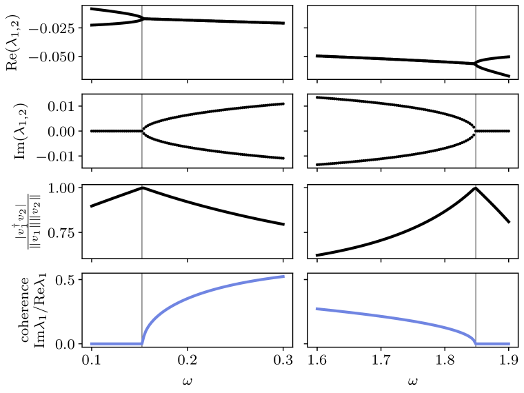
Figure S1: Exceptional point phase transition in the gene switch. We plot two closest to the steady state eigenvalues, and a scalar product of the corresponding eigenvectors as a function of adiabaticity $\omega$. We plot coherence of oscillations for the same parameter range. These plots are made for parameter values $X^{\mathrm{eq}}=X^{\mathrm{ad}}=20$.

B Local winding number in combined bound and unbound chains

In this section we provide equations that are needed to define the local winding number in combined bound and unbound chains in the adiabatic phase. To define a local transition matrix, we choose a unit cell that consists of the $n$-th state in the bound chain and the $(n+1)$-th state in the unbound chain, together with transitions between these states as well as transitions to and from their right neighbors. Under periodic boundary conditions, the local transition matrix is

$$\mathcal{W}^{n,\mathrm{tot}}(\chi)=\begin{pmatrix}(n+1)k(e^{-i\chi}-1)-f&(n+1)h\\ f&g_{1}(e^{i\chi}-1)+(n+2)k(e^{-i\chi}-1)-(n+1)h\end{pmatrix}.$$ (S1)

We compute the combined local winding by plugging this transition matrix in Eq. 1 in the main text.

C Current balance follows from Kirchhoff’s laws

In this section, we derive the current balance principle, which was used in the main text, from the Kirchhoff’s laws. To start, we define the probability current from the $i$-th to the $j$-th state as

$$J_{ji}=\mathcal{W}_{ji}p_{i}-\mathcal{W}_{ij}p_{j}.$$ (S2)

Currents in the gene network must obey the Kirchhoff’s laws:

$$J_{(n+1)0,n0}-J_{n0,(n-1)0} =-J_{(n+1)1,n0},$$ (S3)

$$J_{(n+2)1,(n+1)1}-J_{(n+1)1,n1} =J_{(n+1)1,n0},$$ (S4)

while at the left edge the Kirchhoff’s laws are fulfilled by

$$-J_{10,00}=J_{11,00}=J_{21,11}.$$ (S5)

Summing up Eq. (S3) for $n$ from $1$ to $\infty$, and taking into account Eq. (S5), we derive that the vertical current summed over the network is zero

$$\sum_{n=0}^{\infty}J_{(n+1)1,n0}=0.$$ (S6)

D Analytical derivation of the domain wall in the adiabatic phase

In this section, we analytically derive the domain wall location for the combined local winding number in the adiabatic phase. For this, we use the fact that the winding number changes its sign when currents in the corresponding periodic network vanish [29]. To find this location, we track how vertical and horizontal currents in a local periodic network given by Eq. (S1) change as a function of protein number $n$. Assuming that the total probability in a local network splits into probability $p_{0}$ in the lower chain and $p_{1}$ in the upper chain, we can express the currents in the $(n-1)$-th local network as

$$J_{\mathrm{vertical}} =fp_{0}-nhp_{1},$$ (S7)

$$J_{\mathrm{horizontal}} =J_{0}+J_{1}=-nkp_{0}+(g_{1}-(n+1)k)p_{1},$$ (S8)

where the horizontal current has two contributions, from the lower and the upper chains. To find the domain wall location, we set both vertical and horizontal currents to zero. From $J_{\mathrm{vertical}}=0$ we get

$$p_{0}=nhp_{1}/f.$$ (S9)

Plugging this into $J_{\mathrm{horizontal}}=0$, we get

$$n^{2}+(f/h)n-(f/h)(g_{1}/k-1)=0.$$ (S10)

The positive solution of this equation, parameterized by $X^{\mathrm{ad}}=g_{1}/2k$ and $X^{\mathrm{eq}}=f/h$, is

$$n^{*}_{\mathrm{tot}}=\left(-X^{\mathrm{eq}}+\sqrt{(X^{\mathrm{eq}})^{2}+4X^{\mathrm{eq}}(2X^{\mathrm{ad}}-1)}\right)/2.$$ (S11)

This protein number corresponds to the domain wall of the local winding number.

References

- [1] A. D. Lander, “The edges of understanding,” BMC Biology, vol. 8, p. 40, Dec. 2010.
- [2] M. S. Zaghloul Salem, “Biological Networks: An Introductory Review,” Journal of Proteomics and Genomics Research, vol. 2, pp. 41–111, Oct. 2018.
- [3] A. D. Goldberg, C. D. Allis, and E. Bernstein, “Epigenetics: A Landscape Takes Shape,” Cell, vol. 128, pp. 635–638, Feb. 2007.
- [4] M. Sasai and P. G. Wolynes, “Stochastic gene expression as a many-body problem,” Proceedings of the National Academy of Sciences, vol. 100, pp. 2374–2379, Mar. 2003.
- [5] B. Zhang and P. G. Wolynes, “Topology, structures, and energy landscapes of human chromosomes,” Proceedings of the National Academy of Sciences, vol. 112, pp. 6062–6067, May 2015.
- [6] S. Tripathi, D. A. Kessler, and H. Levine, “Biological Networks Regulating Cell Fate Choice are Minimally Frustrated,” Physical Review Letters, vol. 125, p. 088101, Aug. 2020.
- [7] D. A. Potoyan and P. G. Wolynes, “On the dephasing of genetic oscillators,” Proceedings of the National Academy of Sciences, vol. 111, pp. 2391–2396, Feb. 2014.
- [8] M. Aldana, S. Coppersmith, and L. P. Kadanoff, “Boolean Dynamics with Random Couplings,” in Perspectives and Problems in Nolinear Science: A Celebratory Volume in Honor of Lawrence Sirovich (E. Kaplan, J. E. Marsden, and K. R. Sreenivasan, eds.), pp. 23–89, New York, NY: Springer New York, 2003.
- [9] M. L. Heltberg, S. Krishna, L. P. Kadanoff, and M. H. Jensen, “A tale of two rhythms: Locked clocks and chaos in biology,” Cell Systems, vol. 12, pp. 291–303, Apr. 2021.
- [10] J. Wang, “Landscape and flux theory of non-equilibrium dynamical systems with application to biology,” Advances in Physics, vol. 64, pp. 1–137, Jan. 2015.
- [11] J. Wang, L. Xu, and E. Wang, “Potential landscape and flux framework of nonequilibrium networks: Robustness, dissipation, and coherence of biochemical oscillations,” Proceedings of the National Academy of Sciences, vol. 105, pp. 12271–12276, Aug. 2008.
- [12] K. Zhang, M. Sasai, and J. Wang, “Eddy current and coupled landscapes for nonadiabatic and nonequilibrium complex system dynamics,” Proceedings of the National Academy of Sciences, vol. 110, pp. 14930–14935, Sept. 2013.
- [13] J. E. Moore, “The birth of topological insulators,” Nature, vol. 464, pp. 194–198, Mar. 2010.
- [14] J. Agudo-Canalejo and E. Tang, “Topological phases in discrete stochastic systems,” June 2024. arXiv:2406.03925 [cond-mat, physics:physics].
- [15] M. Z. Hasan and C. L. Kane, “Colloquium : Topological insulators,” Reviews of Modern Physics, vol. 82, pp. 3045–3067, Nov. 2010.
- [16] X.-L. Qi and S.-C. Zhang, “Topological insulators and superconductors,” Reviews of Modern Physics, vol. 83, pp. 1057–1110, Oct. 2011.
- [17] C. L. Kane and T. C. Lubensky, “Topological boundary modes in isostatic lattices,” Nature Physics, vol. 10, pp. 39–45, Jan. 2014.
- [18] S. D. Huber, “Topological mechanics,” Nature Physics, vol. 12, pp. 621–623, July 2016.
- [19] S. Zheng, G. Duan, and B. Xia, “Progress in Topological Mechanics,” Applied Sciences, vol. 12, p. 1987, Feb. 2022.
- [20] L. Lu, J. D. Joannopoulos, and M. Soljačić, “Topological photonics,” Nature Photonics, vol. 8, pp. 821–829, Nov. 2014.
- [21] T. Ozawa, H. M. Price, A. Amo, N. Goldman, M. Hafezi, L. Lu, M. C. Rechtsman, D. Schuster, J. Simon, O. Zilberberg, and I. Carusotto, “Topological photonics,” Reviews of Modern Physics, vol. 91, p. 015006, Mar. 2019.
- [22] F. Serra, U. Tkalec, and T. Lopez-Leon, “Editorial: Topological Soft Matter,” Frontiers in Physics, vol. 8, p. 373, Sept. 2020.
- [23] S. Shankar, A. Souslov, M. J. Bowick, M. C. Marchetti, and V. Vitelli, “Topological active matter,” Nature Reviews Physics, vol. 4, pp. 380–398, May 2022.
- [24] J. Mecke, J. O. Nketsiah, R. Li, and Y. Gao, “Emergent phenomena in chiral active matter,” National Science Open, vol. 3, p. 20230086, Apr. 2024.
- [25] K. Dasbiswas, K. K. Mandadapu, and S. Vaikuntanathan, “Topological localization in out-of-equilibrium dissipative systems,” Proceedings of the National Academy of Sciences, vol. 115, Sept. 2018.
- [26] A. Murugan and S. Vaikuntanathan, “Topologically protected modes in non-equilibrium stochastic systems,” Nature Communications, vol. 8, p. 13881, Apr. 2017.
- [27] J. Knebel, P. M. Geiger, and E. Frey, “Topological Phase Transition in Coupled Rock-Paper-Scissors Cycles,” Physical Review Letters, vol. 125, p. 258301, Dec. 2020.
- [28] E. Tang, J. Agudo-Canalejo, and R. Golestanian, “Topology Protects Chiral Edge Currents in Stochastic Systems,” Physical Review X, vol. 11, p. 031015, July 2021.
- [29] T. Sawada, K. Sone, R. Hamazaki, Y. Ashida, and T. Sagawa, “Role of Topology in Relaxation of One-Dimensional Stochastic Processes,” Physical Review Letters, vol. 132, p. 046602, Jan. 2024.
- [30] A. Nelson and E. Tang, “Nonreciprocity is necessary for robust dimensional reduction and strong responses in stochastic topological systems,” Physical Review B, vol. 110, p. 155116, Oct. 2024.
- [31] C. Zheng and E. Tang, “A topological mechanism for robust and efficient global oscillations in biological networks,” Nature Communications, vol. 15, p. 6453, July 2024.
- [32] J. E. M. Hornos, D. Schultz, G. C. P. Innocentini, J. Wang, A. M. Walczak, J. N. Onuchic, and P. G. Wolynes, “Self-regulating gene: An exact solution,” Physical Review E, vol. 72, p. 051907, Nov. 2005.
- [33] D. Schultz, J. N. Onuchic, and P. G. Wolynes, “Understanding stochastic simulations of the smallest genetic networks,” The Journal of Chemical Physics, vol. 126, p. 245102, June 2007.
- [34] P. J. Choi, X. S. Xie, and E. I. Shakhnovich, “Stochastic Switching in Gene Networks Can Occur by a Single-Molecule Event or Many Molecular Steps,” Journal of Molecular Biology, vol. 396, pp. 230–244, Feb. 2010.
- [35] D. Schultz, A. M. Walczak, J. N. Onuchic, and P. G. Wolynes, “Extinction and resurrection in gene networks,” Proceedings of the National Academy of Sciences, vol. 105, pp. 19165–19170, Dec. 2008.
- [36] Z. Gong, Y. Ashida, K. Kawabata, K. Takasan, S. Higashikawa, and M. Ueda, “Topological Phases of Non-Hermitian Systems,” Physical Review X, vol. 8, p. 031079, Sept. 2018.
- [37] A. C. Barato and U. Seifert, “Coherence of biochemical oscillations is bounded by driving force and network topology,” Physical Review E, vol. 95, p. 062409, June 2017.
- [38] W. van Saarloos, V. Vitelli, and Z. Zeravcic, “Active Matter,” in Soft Matter: Concepts, Phenomena, and Applications, Princeton: Princeton University Press, 1st ed ed., 2024.
- [39] M. Fruchart, R. Hanai, P. B. Littlewood, and V. Vitelli, “Non-reciprocal phase transitions,” Nature, vol. 592, pp. 363–369, Apr. 2021.
- [40] F. E. Öztürk, T. Lappe, G. Hellmann, J. Schmitt, J. Klaers, F. Vewinger, J. Kroha, and M. Weitz, “Observation of a non-Hermitian phase transition in an optical quantum gas,” Science, vol. 372, pp. 88–91, Apr. 2021. Publisher: American Association for the Advancement of Science.
- [41] N. Okuma, K. Kawabata, K. Shiozaki, and M. Sato, “Topological Origin of Non-Hermitian Skin Effects,” Physical Review Letters, vol. 124, p. 086801, Feb. 2020.
- [42] D. S. Borgnia, A. J. Kruchkov, and R.-J. Slager, “Non-Hermitian Boundary Modes and Topology,” Physical Review Letters, vol. 124, p. 056802, Feb. 2020.
- [43] T. Sawada, K. Sone, K. Yokomizo, Y. Ashida, and T. Sagawa, “Bulk-Boundary Correspondence in Ergodic and Nonergodic One-Dimensional Stochastic Processes,” May 2024. arXiv:2405.00458 [cond-mat].
- [44] M. A. Shea and G. K. Ackers, “The 0R Control System of Bacteriophage Lambda: A Physical-Chemical Model for Gene Regulation,” Joural of Molecular Biology, vol. 181, no. 2, pp. 211–230, 1985.
- [45] G. D. Amoutzias, D. L. Robertson, Y. Van De Peer, and S. G. Oliver, “Choose your partners: dimerization in eukaryotic transcription factors,” Trends in Biochemical Sciences, vol. 33, pp. 220–229, May 2008.
- [46] S. T. Smale, “Dimer‐specific regulatory mechanisms within the NF‐κB family of transcription factors,” Immunological Reviews, vol. 246, pp. 193–204, Mar. 2012.
- [47] H. Feng, B. Han, and J. Wang, “Adiabatic and Non-Adiabatic Non-Equilibrium Stochastic Dynamics of Single Regulating Genes,” The Journal of Physical Chemistry B, vol. 115, pp. 1254–1261, Feb. 2011.
- [48] Z. Wang, D. A. Potoyan, and P. G. Wolynes, “Molecular stripping, targets and decoys as modulators of oscillations in the NF-κB/IκBα/DNA genetic network,” Journal of The Royal Society Interface, vol. 13, p. 20160606, Sept. 2016.
- [49] Y. Tu, “The nonequilibrium mechanism for ultrasensitivity in a biological switch: Sensing by Maxwell’s demons,” Proceedings of the National Academy of Sciences, vol. 105, pp. 11737–11741, Aug. 2008.
- [50] T. Lu, T. Shen, C. Zong, J. Hasty, and P. G. Wolynes, “Statistics of cellular signal transduction as a race to the nucleus by multiple random walkers in compartment/phosphorylation space,” Proceedings of the National Academy of Sciences, vol. 103, pp. 16752–16757, Nov. 2006.
Supplemental Material to: Topology of the simplest gene switch
Aleksandra Nelson,1 Peter Wolynes,1, 2, 3, 4 and Evelyn Tang1,3
1Center for Theoretical Biological Physics, Rice University, Houston TX, USA
2Department of Chemistry, Rice University, Houston TX, 77005, USA
3Department of Physics and Astronomy, Rice University, Houston TX, 77005, USA
4Department of Biosciences, Rice University, Houston TX, 77005, USA
(Dated: April 5, 2025)