The Volterra Stein-Stein model with stochastic interest rates

Abstract

We introduce the Volterra Stein-Stein model with stochastic interest rates, where both volatility and interest rates are driven by correlated Gaussian Volterra processes. This framework unifies various well-known Markovian and non-Markovian models while preserving analytical tractability for pricing and hedging financial derivatives. We derive explicit formulas for pricing zero-coupon bond and interest rate cap or floor, along with a semi-explicit expression for the characteristic function of the log-forward index using Fredholm resolvents and determinants. This allows for fast and efficient derivative pricing and calibration via Fourier methods. We calibrate our model to market data and observe that our framework is flexible enough to capture key empirical features, such as the humped-shaped term structure of ATM implied volatilities for cap options and the concave ATM implied volatility skew term structure (in log-log scale) of the S&P 500 options. Finally, we establish connections between our characteristic function formula and expressions that depend on infinite-dimensional Riccati equations, thereby making the link with conventional linear-quadratic models.

Keywords: Gaussian Volterra processes, volatility, interest rate, memory, Fredholm resolvents and determinants, Fourier pricing, Riccati equations.

1 Introduction

Modeling the joint dynamics of interest rates and equity is crucial for pricing and hedging hybrid derivatives. These products, which include equity-linked interest rate derivatives, callable hybrid structures, and quanto options, depend on the interaction between stock prices, interest rates, and their volatilities. A realistic model must capture the well-documented stylized facts of each underlying as well as accurately describe their dependency structure to ensure consistent pricing and risk management across asset classes.

Empirical evidence reveals persistent memory effects in historical time series of interest rates and asset volatility and slow decay of their autocorrelations structures, see Cont (2001); Dai and Singleton (2003); McCarthy, DiSario, Saraoglu, and Li (2004).

Beyond historical data, robust and universal patterns emerge in the term structures of option prices across a broad range of maturities. Specifically,

1. for interest rates: the term structure of the implied volatilities of cap and floor options is typically hump-shaped, with a steep increase at short maturities followed by a more gradual decay at longer maturities, see for instance Dai and Singleton (2003); De Jong, Driessen, and Pelsser (2004);

2. for stock indices such as the S&P 500: the term structure of the At-The-Money (ATM) skew of the implied volatility of call and put options, when plotted in log-log scale, exhibits typically a concave shape. In addition, the ATM skew displays an approximately linear decrease at long maturities suggesting a power-law decay, though only for sufficiently large maturities, see Abi Jaber and Li (2024); Bayer, Friz, and Gatheral (2016); Bergomi (2015); Delemotte, De Marco, and Segonne (2023); Guyon and El Amrani (2023).

Various approaches have been developed to jointly model equity and interest rate dynamics, often by extending stochastic volatility frameworks to include stochastic interest rates. For instance, Singor, Grzelak, van Bragt, and Oosterlee (2013); Grzelak, Oosterlee, and Van Weeren (2011) incorporated stochastic rates into the Heston (1993) model, while van Haastrecht et al. (2009); van Haastrecht and Pelsser (2011) adapted the Stein and Stein (1991) and Schöbel and Zhu (1999) volatility models with multi-factor Hull and White (1993) interest rates. However, these frameworks rely on Markovian dynamics with a single characteristic time scale for at least one of the two risk factors, and fail to capture the complex shapes of term structures observed on the market: they lead either to term structures of cap/floor implied volatilities that decrease monotonically - at odds with the empirically observed hump-shaped patterns - or ATM skews that decay too quickly for longer maturities. While such models offer analytical tractability, their inability to align with empirical data highlights the need for alternative approaches that incorporate more flexibility.

To address these limitations, we propose a flexible yet analytically tractable model based on Volterra processes, capable of accurately reproducing these empirical term structure features while remaining computationally efficient for option pricing and model calibration. Our motivation for incorporating Volterra processes stems from their proven ability to capture key stylized facts of volatility (Abi Jaber and Li (2024); Bayer, Friz, and Gatheral (2016); Gatheral, Jaisson, and Rosenbaum (2018); Guyon and Lekeufack (2023)) and interest rates (Abi Jaber (2022b); Benth and Rohde (2019); Corcuera, Farkas, Schoutens, and Valkeila (2013); Hainaut (2022)).

We propose a hybrid equity-rate modeling framework where both volatility and interest rates are driven by (possibly correlated) Gaussian Volterra processes, unifying a broad class of Markovian and non-Markovian models. Building on the Volterra Stein-Stein model with constant interest rates studied by Abi Jaber (2022a), we extend the framework to incorporate stochastic interest rates, capturing key market features more effectively. Our main contributions can be summarized as follows:

• Mathematical tractability and pricing: Despite the non-Markovian nature of the processes, we derive explicit pricing formulas for zero-coupon bonds and call and put options on zero-coupon bonds, see Propositions 2.1 and 2.2. We obtain a semi-explicit expression for the characteristic function of the log-forward index in terms of Fredholm (1903) resolvents and determinants, enabling Fourier-based pricing methods, see Theorem 3.1. This result extends the formula derived by Abi Jaber (2022a) for constant interest rates.

• Flexibility and joint calibration: We calibrate our model to market data and achieve excellent fits for: (i) the humped-shaped term structure of ATM implied volatilities for cap options by incorporating in interest rates mean reversion as well as long-range memory with a fractional kernel, see Figure 3, and (ii) the concave ATM implied volatility skew term structure (in a log-log plot) of S&P 500 options using a shifted fractional kernel, see Figure 8. On the selected calibration date, our estimated parameters yield a negative implied correlation between short rates and the index, aligning with historical observations. Furthermore, we compare the impact of a singular power-law kernel for volatility (rough volatility) and demonstrate that rough models underperform our non-rough counterparts in capturing the entire volatility surface, confirming within our framework the findings of Abi Jaber and Li (2024); Delemotte, De Marco, and Segonne (2023); Guyon and Lekeufack (2023).

• Link with conventional linear-quadratic models: We establish connections between our characteristic function formula and expressions that depend on infinite-dimensional Riccati equations, see Proposition 5.1 for general kernels and Proposition 5.2 for completely monotone convolution kernels. The latter formula establishes the link with conventional linear-quadratic models (Proposition 5.3), allows us to recover closed-form solutions in specific cases such as in van Haastrecht, Lord, Pelsser, and Schrager (2009) (Corollary 5.1), and leads to another numerical approximation method based on multi-factor approximations in the spirit of Abi Jaber and El Euch (2019), see Section 5.3.

The paper is outlined as follows. In Section 2, we introduce the Volterra Stein-Stein model with stochastic rates, derive pricing formulas for zero-coupon bonds, and analyze the forward index dynamics. Section 3 provides a semi-explicit expression for the characteristic function of the log-index. In Section 4, we validate the Gaussian Volterra framework by calibrating the interest rate and volatility models to market data. Finally, Section 5 establishes connections with conventional linear-quadratic models, derives simplified forms for Markovian volatility models, and introduces a multi-factor approximation for the characteristic function for completely monotone kernels.

2 The Volterra Stein-Stein and Hull-White model

We fix a finite horizon $T>0$ and a filtered probability space $(\Omega,\mathcal{F},(\mathcal{F}_{t})_{0\leq t\leq T},\mathbb{Q})$ where $\mathbb{Q}$ stands for one risk-neutral probability measure and the filtration $(\mathcal{F}_{t})_{0\leq t\leq T}$ satisfies the usual conditions. We consider a financial market with a financial index denoted by $(I_{t})_{0\leq t\leq T}$ that depends on both stochastic interest rate $(r_{t})_{0\leq t\leq T}$ and volatility $(\nu_{t})_{0\leq t\leq T}$ with dynamics

$$dI_{t}=r_{t}\>I_{t}\>dt+\nu_{t}I_{t}\>dW_{I}^{\mathbb{Q}}(t).$$

In order to incorporate memory effects, we model the two risk factors $(\nu,r)$ by general Gaussian Volterra processes, combining a Volterra Stein-Stein model for $\nu$, as studied by Abi Jaber (2022a), with a Volterra Hull-White model for $r$:

$$r_{t} =r_{0}(t)+\int_{0}^{t}G_{r}(t,s)\kappa_{r}\>r_{s}ds+\int_{0}^{t}G_{r}(t,s)\>\eta_{r}\>dW_{r}^{\mathbb{Q}}(s),$$ (2.1)

$$\nu_{t} =g_{0}(t)+\int_{0}^{t}G_{\nu}(t,s)\kappa_{\nu}\>\nu_{s}ds+\int_{0}^{t}G_{\nu}(t,s)\>\eta_{\nu}\>dW_{\nu}^{\mathbb{Q}}(s)$$ (2.2)

where $(W_{I}^{\mathbb{Q}},W_{r}^{\mathbb{Q}},W_{\nu}^{\mathbb{Q}})$ are correlated Brownian motions such that

$$d\langle W_{l}^{\mathbb{Q}},W_{k}^{\mathbb{Q}}\rangle_{t}=\rho_{lk}\>dt,$$

with $\rho_{lk}\in[-1,1],\>l,k\in\{I,r,\nu\}$, $\kappa_{r},\kappa_{\nu}\in\mathbb{R}$, $\eta_{r},\eta_{\nu}\in\mathbb{R}$, and the kernels $G_{r}(.)$ and $G_{\nu}(.)$ satisfy the following definition.

Definition 2.1.

A kernel $G:[0,T]^{2}\to\mathbb{R}$ is a Volterra kernel of continuous and bounded type in $L^{2}$ if $G(t,s)=0$ for $s\geq t$ and

$$\sup_{t\leq T}\int_{0}^{T}\left(|G(t,s)|^{2}+|G(s,t)|^{2}\right)ds<+\infty,\quad\lim_{h\to 0}\int_{0}^{T}|G(u+h,s)-G(u,s)|^{2}ds=0,\quad u\leq T.$$

Finally, $r_{0}(.)$ is a time-dependent function used to perfectly fit the initial term-structure of market bond prices, see Remark 2.1, and $g_{0}$ is such that

$$g_{0}(t)=\nu_{0}+\theta_{\nu}\int_{0}^{t}G_{\nu}(t,s)ds,\quad\nu_{0}\in\mathbb{R}_{+},\>\theta_{\nu}\in\mathbb{R}.$$ (2.3)

Under Definition 2.1 and for $r_{0},g_{0}$ locally square integrable, it can be shown there exists a strong solution to (2.1) and (2.2), such that

$$\sup_{0\leq t\leq T}\mathbb{E}^{\mathbb{Q}}\left[|r_{t}|^{p}+|\nu_{t}|^{p}\right]<+\infty,\quad p\geq 1,$$

this follows from an adaption of (Abi Jaber, 2022a, Theorem A.3). In particular, the joint process $(r,\nu)$ is a Gaussian process.

This class of models encompasses well-known Markov and non-Markovian Volterra processes. For an introduction to Volterra processes, we refer among others to (Hainaut, 2022, Chapter 9). Several kernels satisfy Definition 2.1 such as:

• the constant kernel: $G(t,s)=1_{s<t}$, then we obtain Markovian models such as the classical Stein and Stein (1991) or Schöbel and Zhu (1999) model for volatility and the Hull and White (1993) model for short-term interest rate, such models have been studied by van Haastrecht, Lord, Pelsser, and Schrager (2009); Grzelak, Oosterlee, and Van Weeren (2012),

• the exponential kernel: $G(t,s)=1_{s<t}\exp(-\beta(t-s))$ with $\beta\in\mathbb{R}_{+}$, then we also obtain Markovian models but with modified mean-reversion level and reversion speed,

• the fractional kernel: $G(t,s)=1_{s<t}(t-s)^{H-1/2}$ with a Hurst index $H\in(0,1)$ then we obtain non-semimartingale and non-Markovian long or short memory fractional processes whenever $H\neq 1/2$. For $H<1/2,$ the kernel is singular at $t\to s$, we get rough models as for example the rough Stein-Stein model studied by Abi Jaber (2022a) and for $H>1/2$, we obtain long-memory processes as, for example, the fractional version of the Hull and White model,

• the shifted fractional kernel: $G(t,s)=1_{s<t}(t-s+\varepsilon)^{H-1/2},$ with $\varepsilon>0$ and $H\in\mathbb{R}$, then we obtain path-dependent processes that are semi-martingales but non-Markovian processes. Compared to the fractional kernel, the shifted fractional kernel has no singularity as $t\to s$, and can achieve faster decays than the fractional kernel for larger $t$ with coefficients $H\leq 0$.

2.1 Pricing Zero-Coupon bonds and interest rate derivatives

Let us now consider the pricing of zero-coupon bond as well as interest rate derivatives in our framework. The price at time $t\leq T$ of a $T-$maturity zero-coupon bound is denoted by $P(t,T)$ and defined by

$$P(t,T)=\mathbb{E}^{\mathbb{Q}}\left[e^{-\int_{t}^{T}r_{s}ds}\mid\mathcal{F}_{t}\right].$$

We now show that even considering a general Volterra Hull and White model for interest rate dynamics, the zero-coupon bond price admits an analytic expression. To this end, we introduce the concept of resolvent associated to a kernel and give some examples in Table 1. Note that we consider the resolvent definition of Abi Jaber (2022a), which may differ from other papers.

Definition 2.2.

Let $G$ be a kernel satisfying Definition 2.1. The resolvent of $G$ is the kernel $R_{G}$ satisfying Definition 2.1 and such that

$$R_{G}=G+G\star R_{G},$$

where the $\star-$product is such that, for $(s,w)\in[0,T]^{2},$

$$(G\star R_{G})(s,w)=\int_{0}^{T}G(s,z)R_{G}(z,w)dz.$$

Kernel $G(t,s)$	Resolvent $R_{G}(t,s)$	$B_{G}(t,T)=\int_{t}^{T}R_{G}(s,t)ds$
$1_{s<t}\>c$	$1_{s<t}\>ce^{c(t-s)}$	$e^{c(T-t)}-1$
$1_{s<t}\>c\exp(-\beta(t-s))$	$1_{s<t}\>ce^{(t-s)(c-\beta)}$	$\frac{c}{c-\beta}(e^{(c-\beta)(T-t)}-1)$
$1_{s<t}\>c\frac{(t-s)^{\alpha-1}}{\Gamma(\alpha)}$	$1_{s<t}\>c(t-s)^{\alpha-1}E_{\alpha,\alpha}(c(t-s)^{\alpha})$	$c(T-t)^{\alpha}E_{\alpha,\alpha+1}(c(T-t)^{\alpha})$

Table 1: Particular kernels, the associated resolvents and the integral of these resolvents where $E_{\beta,\gamma}(x)=\sum_{n=0}^{\infty}\frac{x^{n}}{\Gamma(n\beta+\gamma)}$.

Proposition 2.1.

Let us define, for $t\in[0,T],$ $f_{t}(.)$ by

$$f_{t}(s):=r_{0}(s)+\int_{0}^{t}R_{\kappa_{r}G_{r}}(s,u)r_{0}(u)du+\frac{\eta_{r}}{\kappa_{r}}\int_{0}^{t}R_{\kappa_{r}G_{r}}(s,u)\;dW_{r}^{\mathbb{Q}}(u),\;t\leq s,$$ (2.4)

with $R_{\kappa_{r}G_{r}}$ the resolvent associated to $\kappa_{r}G_{r}$ with the convention $\frac{R_{\kappa_{r}G_{r}}}{\kappa_{r}}=G_{r}$ if $\kappa_{r}=0$. The price of the zero-coupon bond at time $t\in[0,T],$ is given by

$$P(t,T)=A(t,T)\exp\bigg{(}-\int_{t}^{T}f_{t}(s)\>ds\bigg{)},$$ (2.5)

with $A(t,T)$ the time-dependent function given by

$$A(t,T):=\exp\bigg{(}-\int_{t}^{T}\bigg{(}\int_{u}^{T}R_{\kappa_{r}G_{r}}(s,u)r_{0}(u)ds+\frac{\eta_{r}^{2}}{2}B_{G_{r}}^{2}(u,T)\>\bigg{)}\>du\bigg{)}.$$

Moreover, the dynamics of ($P(t,T))_{t\in[0,T]}$ are given by

$$\frac{dP(t,T)}{P(t,T)}=r_{t}\>dt-\eta_{r}B_{G_{r}}(t,T)dW_{r}^{\mathbb{Q}}(t),$$

with

$$B_{G_{r}}(t,T):=\frac{1}{\kappa_{r}}\int_{t}^{T}R_{\kappa_{r}G_{r}}(s,t)\;ds.$$ (2.6)

Proof.

Using the resolvent associated to the kernel $\kappa_{r}G_{r}$ and using (Abi Jaber, 2022a, Theorem A.3), we have that $(r_{t})_{0\leq t\leq T}$ is the strong solution of the following equation

$$r_{t}=r_{0}(t)+\int_{0}^{t}R_{\kappa_{r}G_{r}}(t,s)r_{0}(s)ds+\frac{1}{\kappa_{r}}\int_{0}^{t}R_{\kappa_{r}G_{r}}(t,s)\eta_{r}\;dW_{r}^{\mathbb{Q}}(s),\>0\leq t\leq T,$$

with the convention $\frac{R_{\kappa_{r}G_{r}}}{\kappa_{r}}=G_{r}$ if $\kappa_{r}=0.$ In this case, we have that, for $0\leq t\leq T,$

$$\int_{t}^{T}r_{s}ds=\int_{t}^{T}r_{0}(s)ds+\int_{t}^{T}\int_{0}^{s}R_{\kappa_{r}G_{r}}(s,u)r_{0}(u)\>duds+\frac{1}{\kappa_{r}}\int_{t}^{T}\int_{0}^{s}R_{\kappa_{r}G_{r}}(s,u)\eta_{r}\;dW_{r}^{\mathbb{Q}}(u)ds.$$

Using the definition of $f_{t}$ given by (2.4) together with an application of stochastic Fubini’s theorem, we obtain that

$$\int_{t}^{T}r_{s}ds=\int_{t}^{T}f_{t}(s)ds+\int_{t}^{T}\int_{u}^{T}R_{\kappa_{r}G_{r}}(s,u)r_{0}(u)dsdu+\eta_{r}\int_{t}^{T}\underbrace{\frac{1}{\kappa_{r}}\int_{u}^{T}R_{\kappa_{r}G_{r}}(s,u)\;ds}_{:=B_{G_{r}}(u,T)}dW_{r}^{\mathbb{Q}}(u).$$

Thus, for $t\in[0,T],$ conditional on $\mathcal{F}_{t}$, the random variable $\int_{t}^{T}r_{s}ds|$ is Gaussian with mean

$$\mathbb{E}^{\mathbb{Q}}\left[\int_{t}^{T}r_{s}ds\mid\mathcal{F}_{t}\right]=\int_{t}^{T}f_{t}(s)ds+\int_{t}^{T}\int_{u}^{T}R_{\kappa_{r}G_{r}}(s,u)r_{0}(u)dsdu,$$

and variance

$$\mathbb{V}^{\mathbb{Q}}\left[\int_{t}^{T}r_{s}ds\mid\mathcal{F}_{t}\right]=\eta_{r}^{2}\int_{t}^{T}B_{G_{r}}^{2}(u,T)\>du.$$

Therefore, we readily deduce that

$$P(t,T)=\exp\bigg{(}-\int_{t}^{T}f_{t}(s)ds-\int_{t}^{T}\bigg{(}\int_{u}^{T}R_{\kappa_{r}G_{r}}(s,u)r_{0}(u)ds+\frac{\eta_{r}^{2}}{2}B_{G_{r}}^{2}(u,T)\>\bigg{)}\>du\bigg{)},$$

and we finally obtain that

$$\frac{dP(t,T)}{P(t,T)}=r_{t}dt-\eta_{r}\int_{t}^{T}\frac{1}{\kappa_{r}}R_{\kappa_{r}G_{r}}(s,t)ds\>dW_{r}^{\mathbb{Q}}(t).$$

∎

Remark 2.1.

Proposition 2.1 provides a natural way to estimate the function $r_{0}(.)$ such that the interest rate model matches perfectly the initial term-structure of market bond prices. In fact from (2.5), we deduce that

$$\int_{0}^{t}r_{0}(s)\>\bigg{(}1+\kappa_{r}B_{G_{r}}(s,t)\bigg{)}\>ds=-\ln P(0,t)-\int_{0}^{t}\frac{\eta_{r}^{2}}{2}B_{G_{r}}^{2}(s,t)\>ds.$$

Thus, if we assume that, for some given maturities $0=T_{0}<T_{1}<...<T_{n}$, we have the initial term-structure of market bond prices $P^{Market}(0,T_{i})$, and that $r_{0}(t)$ is piecewise constant such that

$$r_{0}(t)=-\frac{\ln P^{Market}(0,T_{i})-\ln P^{Market}(0,T_{i-1})+\frac{\eta_{r}^{2}}{2}\int_{T_{i-1}}^{T_{i}}B_{G_{r}}^{2}(u,T_{i})\>du}{(T_{i}-T_{i-1})+\kappa_{r}\int_{T_{i-1}}^{T_{i}}B_{G_{r}}(s,T_{i})\,ds},\>t\in[T_{i-1},T_{i}),$$ (2.7)

then $P(0,T_{i})=P^{Market}(0,T_{i}),\>i=1,...,n.$ $\square$

Based on the expression for the pricing of zero-coupon bonds, we can now easily deduce explicit expressions for the pricing of zero-coupon bond call and put options.

Proposition 2.2.

Let us consider $T-$maturity zero-coupon bond call option $(P(T,S)-K)_{+}$ and put option $(K-P(T,S))_{+}$ with $S>T$ and $K$ the strike of the option. The arbitrage-free price at time $t\in[0,T]$ of the call option is given by

$$\text{Call}_{ZC}(t,T,S,K)=P(t,S)\phi(-d_{1}(t,T))-KP(t,T)\phi(-d_{2}(t,T)),$$

and the price of the put option is given by

$$\text{Put}_{ZC}(t,T,S,K)=KP(t,T)\phi(d_{2}(t,T))-P(t,S)\phi(d_{1}(t,T)),$$

where $\phi(.)$ is the cumulative function of a normal distribution and

$$d_{1}(t,T)=d_{2}(t,T)-v(t,T,S),$$ (2.8)

$$d_{2}(t,T)=\frac{1}{v(t,T,S)\sqrt{T-t}}\log\bigg{(}\frac{KP(t,T)}{P(t,S)}\bigg{)}+\frac{v(t,T,S)\sqrt{T-t}}{2},$$ (2.9)

where

$$v(t,T,S)^{2}=\frac{\eta_{r}^{2}\int_{t}^{T}\bigg{(}B_{G_{r}}(s,T)-B_{G_{r}}(s,S)\bigg{)}^{2}ds.}{T-t}$$ (2.10)

Proof.

Let us consider the call option. We know that the arbitrage-free price of a call on zero-coupon bond satisfies

$$\text{Call}_{ZC}(t,T,S,K)=P(t,T)\mathbb{E}^{\mathbb{Q}^{T}}\left[(P(T,S)-K)_{+}\mid\mathcal{F}_{t}\right].$$

From Proposition 2.1, we know that under the risk-neutral measure $\mathbb{Q},$

$$\frac{dP(t,S)}{P(t,S)}=r_{t}\>dt-\eta_{r}B_{G_{r}}(t,S)dW_{r}(t).$$

Therefore, for $S>T,$ we obtain that under the $T-$forward measure $\mathbb{Q}^{T}$, the zero-coupon bond dynamics is given by

$$\frac{dP(t,S)}{P(t,S)}=\bigg{(}r_{t}+\eta_{r}^{2}B_{G_{r}}(t,S)B_{G_{r}}(t,T)\bigg{)}\>dt-\eta_{r}B_{G_{r}}(t,S)dW_{r}^{\mathbb{Q}^{T}}(t).$$

Moreover, under $\mathbb{Q}^{T},$ we have that

$$d\bigg{(}\frac{P(t,S)}{P(t,T)}\bigg{)}=\frac{P(t,S)}{P(t,T)}\eta_{r}\bigg{(}B_{G_{r}}(t,T)-B_{G_{r}}(t,S)\bigg{)}dW_{r}^{\mathbb{Q}^{T}}(t)$$

and we deduce that

$$\mathbb{E}^{\mathbb{\mathbb{Q}}^{T}}\left[(P(T,S)-K)_{+}\mid\mathcal{F}_{t}\right]=\frac{P(t,S)}{P(t,T)}\phi(-d_{1}(t,T))-K\phi(-d_{2}(t,T)),$$

where $\phi(.)$ is the cumulative function of a normal distribution and $d_{1},d_{2}$ are given by (2.8)-(2.9). Finally, using the call/put parity, we easily deduce the form of the put price. ∎

Based on zero-coupon bonds call or put options, we can price cap and floor options since, as explained in Brigo and Mercurio (2006), cap and floor options can be decomposed into a sum of zero-coupon bonds options. In fact, the cap and floor payoffs are of the form

$$\text{Cap}=\sum_{i=1}^{\beta}(T_{i}-T_{i-1})\>(L(T_{i-1},T_{i})-K)_{+},$$

$$\text{Floor}=\sum_{i=1}^{\beta}(T_{i}-T_{i-1})\>(K-L(T_{i-1},T_{i}))_{+}$$

where $L$ is the reference rate and $(T_{1},...,T_{\beta})$ are the payment date. Using Brigo and Mercurio (2006), we have that the price at time $t<T_{0}$, of cap and floor options is given by

$$\text{Cap}(t,\beta,K)=\sum_{i=1}^{\beta}(1+K(T_{i}-T_{i-1}))\>\text{Put}_{ZC}\left(t,T_{i-1},T_{i},\frac{1}{1+K(T_{i}-T_{i-1})}\right).$$

$$\text{Floor}(t,\beta,K)=\sum_{i=1}^{\beta}(1+K(T_{i}-T_{i-1}))\>\text{Call}_{ZC}\left(t,T_{i-1},T_{i},\frac{1}{1+K(T_{i}-T_{i-1})}\right).$$

This enable us to calibrate our Gaussian Volterra model for interest rate to the market data of cap and floor options for any Volterra kernel $G_{r}(.)$.

2.2 Forward measure and pricing of derivatives on the index

Let us now focus on the pricing financial derivatives on the index $I$ in our framework. Standard arguments imply that the arbitrage-free price of financial derivatives is obtained by taking the discounted value of the payoffs under a risk-neutral measure $\mathbb{Q}$. In this case, if we consider a general $T-$maturity derivative of the form

$$H_{T}:=h(I_{T})\in L^{2}(\mathbb{Q}),$$

where $h(.)$ is a continuous positive function, the arbitrage-free price at time $t\in[0,T],$ is given by

$$V_{t}=\mathbb{E}^{\mathbb{Q}}\left[e^{-\int_{t}^{T}r_{s}ds}H_{T}\mid\mathcal{F}_{t}\right].$$ (2.11)

In the presence of stochastic interest rates, it is impossible to obtain a more explicit form of the price if we consider the formulation under the risk-neutral measure. One technique for dealing with this problem is to switch from the risk-neutral measure to the $T-$forward neutral measure. Thus, let us introduce the $T-$forward neutral measure denoted by $\mathbb{Q}^{T}$ which is equivalent to the risk-neutral measure $\mathbb{Q}$. The change of measure from the risk-neutral measure $\mathbb{Q}$ to the $T-$forward measure $\mathbb{Q}^{T}$ satisfies

$$\frac{d\mathbb{Q}^{T}}{d\mathbb{\mathbb{Q}}}\bigg{|}_{t}:=e^{-\int_{0}^{t}r(s)\>ds}\frac{P(t,T)}{P(0,T)}.$$

We can now introduce the $T-$forward index denoted by $(I_{t}^{T})_{0\leq t\leq T}$ and defined as, for $0\leq t\leq T,$

$$I_{t}^{T}:=\mathbb{E}^{\mathbb{Q}^{T}}\left[I_{T}\mid\mathcal{F}_{t}\right]=\frac{I_{t}}{P(t,T)}.$$

Since under the forward measure the financial index divided by the zero-coupon bond is a martingale, we obtain that the process $(I_{t}^{T})_{0\leq t\leq T}$ has the following dynamic

$$\frac{dI_{t}^{T}}{I_{t}^{T}}=\nu_{t}\>dW_{I}^{\mathbb{Q}^{T}}(t)+\eta_{r}B_{G_{r}}(t,T)\>dW_{r}^{\mathbb{Q}^{T}}(t),$$ (2.12)

with

$$\nu_{t}=g_{0}^{T}(t)+\int_{0}^{t}G_{\nu}(t,s)\kappa_{\nu}\>\nu_{s}ds+\int_{0}^{t}G_{\nu}(t,s)\>\eta_{\nu}\>dW_{\nu}^{\mathbb{Q}^{T}}(s),$$ (2.13)

where $(W_{r}^{\mathbb{Q}^{T}},W_{I}^{\mathbb{Q}^{T}},W_{\nu}^{\mathbb{Q}^{T}})$ is a $3-$dimensional correlated Brownian motion under the $T-$forward measure $\mathbb{Q}^{T}$ and

$$g_{0}^{T}(t)=g_{0}(t)-\eta_{\nu}\eta_{r}\rho_{r\nu}\int_{0}^{t}G_{\nu}(t,s)\>B_{G_{r}}(s,T)\>ds.$$

By combining the forward measure and the $T-$forward financial index, we obtain that the arbitrage-free price of a derivative (2.11) satisfies

$$V_{t}=P(t,T)\mathbb{E}^{\mathbb{Q}^{T}}\left[\,h(e^{\log I_{T}^{T}})\,\mid\mathcal{F}_{t}\right].$$

By switching from the risk-neutral measure to the $T-$forward measure, we get a simpler framework for pricing financial derivatives. In the following, we will show that the characteristic function of the log-forward index $(\log I_{t}^{T})_{0\leq t\leq T}$ admits an explicit form. This opens the way to a fast pricing of financial derivatives using Fourier methods. Moreover, using hedging approaches developed in several papers Abi Jaber and Gérard (2024); El Euch and Rosenbaum (2018); Motte and Hainaut (2024), some hedging strategies can also be deduced by Fourier methods for contingent claims that admit a Fourier representation.

3 The characteristic function of the log-forward index

The aim of this section is to derive an analytical form of the characteristic function of the log-forward index $(I_{t}^{T})_{0\leq t\leq T}$ with dynamics (2.12) under $\mathbb{Q}^{T}$ and apply it for Fourier pricing of derivatives on the index.

We start by recalling some results on operator theory in Hilbert spaces as well as introducing some notations. Let $\mathbf{A}$ be a linear compact operator acting on $L^{2}([0,T],\mathbb{C})$. Then, $\mathbf{A}$ is a bounded operator i.e. there exists $C>0$ such that, for all $f\in L^{2}([0,T],\mathbb{C})$, $||\mathbf{A}f||\leq C||f||$ and for $B:=\{f\in L^{2}([0,T],\mathbb{C}):||f||\leq 1\}$, the closure of $\mathbf{A}(B)$ is compact in $L^{2}([0,T],\mathbb{C})$. $\mathbf{A}$ is an integral operator if $\mathbf{A}$ a linear operator induced by a kernel $G\in L^{2}([0,T]^{2},\mathbb{R})$ such that, for $f\in L^{2}([0,T],\mathbb{C})$ and $s\in[0,T],$

$$(\mathbf{A}f)(s)=\int_{0}^{T}G(s,w)f(w)dw.$$

Moreover, if $\mathbf{A}$ is a integral operator, then $\mathbf{A}$ is a Hilbert-Schmidt operator on $L^{2}([0,T],\mathbb{C})$ into itself and is in particular compact. The trace of an operator, denoted by $\text{Tr}(.)$, is defined for operators of trace class where a compact operator $\mathbf{A}$ is said to be of trace class if

$$\text{Tr}(\mathbf{A})=\sum_{n\geq 1}\langle\mathbf{A}v_{n},v_{n}\rangle<\infty,$$

for a given orthonormal basis $(v_{n})_{n\geq 1}$. For more details about the trace of an operator, we refer to (Abi Jaber, 2022a, Section A) and the references therein.

Let us now introduce some notations and properties:

• $\langle\cdot,\cdot\rangle_{L^{2}}$ denotes the following product on $L^{2}([0,T],\mathbb{C})$

  $$\langle f,g\rangle_{L^{2}}=\int_{0}^{T}f(s)g(s)ds,\quad f,g\in L^{2}([0,T],\mathbb{C}).$$

  Note that $\langle\cdot,\cdot\rangle_{L^{2}}$ is the inner product in $L^{2}([0,T],\mathbb{R})$ but not in $L^{2}([0,T],\mathbb{C})$.

• For any kernels $G_{1},G_{2}\in L^{2}([0,T]^{2},\mathbb{\mathbb{R}}),$ the $\star-$product is defined by

  $$(G_{1}\star G_{2})(s,w)=\int_{0}^{T}G_{1}(s,z)G_{2}(z,w)dz,\quad(s,w)\in[0,T]^{2}.$$

• For a kernel $G,$ $G^{*}$ denotes the adjoint kernel such that, for $(s,w)\in[0,T]^{2},$

  $$G^{*}(s,w)=G(w,s),$$

  and $\mathbf{G}^{*}$ is the operator induced by $G^{*}.$

• id denotes the identity operator such that $(\text{id}f)=f$, $f\in L^{2}([0,T],\mathbb{C})$.

3.1 Semi-explicit expression

We now derive a semi-explicit form for the characteristic function of the log-forward index in our framework.

To this end, we consider an approach similar to Abi Jaber (2022a) which deduces the explicit form of the log-price characteristic function in equity markets with a Volterra Stein-Stein volatility model. Here, we show that this result can be extended to a framework where interest rates are also stochastic. As in Abi Jaber (2022a), we consider the expression of the adjusted conditional mean of $\nu_{t}$ and then we define a linear operator $\mathbf{\Psi}_{t}^{u}$ in $L^{2}([0,T],\mathbb{C})$ that will be useful for the expression of the characteristic function. The adjusted conditional mean of $\nu_{t}$ denoted by $g_{t}$ is given by

$$g_{t}(s)=1_{t\leq s}\mathbb{E}^{\mathbb{Q}^{T}}\left[\nu_{s}-\int_{t}^{T}G_{\nu}(s,w)\kappa_{\nu}\nu_{w}dw\mid\mathcal{F}_{t}\right],\quad s,t\leq T,$$

and we can easily show that $g_{t}$ reduces to

$$g_{t}(s)=1_{t\leq s}\bigg{(}g_{0}^{T}(s)+\int_{0}^{t}G_{\nu}(s,w)\kappa_{\nu}\nu_{w}dw+\int_{0}^{t}G_{\nu}(s,w)\eta_{\nu}\>dW_{\nu}^{\mathbb{Q}^{T}}(w)\bigg{)},\quad s,t\leq T.$$

Definition 3.1.

For $u\in\mathbb{C}$ such that $0\leq\mathcal{\mathfrak{R}}(u)\leq 1,$ the operator $\mathbf{\Psi}_{t}^{u}$ acting on $L^{2}([0,T],\mathbb{C})$ is defined by

$$\mathbf{\Psi}_{t}^{u}:=(\text{id}-b^{u}\mathbf{G}_{\nu}^{*})^{-1}a^{u}(\text{id}-2a^{u}\tilde{\mathbf{\Sigma}}_{t}^{u})^{-1}(\text{id}-b^{u}\mathbf{G}_{\nu})^{-1},\quad t\leq T,$$ (3.1)

where:

• $\mathbf{G}_{\nu}$ is the integral operator induced by $G_{\nu}(.)$ and $\mathbf{G}_{\nu}^{*}$ the adjoint operator,

• $a^{u}:=\frac{1}{2}(u^{2}-u)$ and $b^{u}:=\kappa_{\nu}+\eta_{\nu}u\rho_{I\nu},$

• $\tilde{\mathbf{\Sigma}}_{t}^{u}$ is the adjusted covariance integral operator such that

  $$\tilde{\mathbf{\Sigma}}_{t}^{u}=(\text{id}-b^{u}\mathbf{G}_{\nu})^{-1}\mathbf{\Sigma}_{t}(\text{id}-b^{u}\mathbf{G}_{\nu}^{*})^{-1},$$

  with $\mathbf{\Sigma_{t}}$ the integral operator associated with the covariance kernel given by

  $$\Sigma_{t}(s,w)=\eta_{\nu}^{2}\int_{t}^{T}G_{\nu}(s,z)G_{\nu}(w,z)dz,\;t\leq s,u\leq T.$$

Note that using similar arguments than in the proof of (Abi Jaber et al., 2021a, Lemma 5.6.), we can prove that $\mathbf{\Psi}_{t}^{u}$ is well defined and is a bounded linear operator acting on $L^{2}([0,T],\mathbb{C})$.

Based now on $g_{t}$ and $\mathbf{\Psi}_{t}^{u}$, we deduce a semi-explicit expression of the characteristic function. The methodology used in Abi Jaber (2022a) to deduce the analytical expression of the characteristic function can be extended to a framework with stochastic interest rates. Nevertheless, to extend these results, we need to consider the process $h_{t}^{u}(.)$ defined, for $u\in\mathbb{C}$ such that $0\leq\mathcal{\mathfrak{R}}(u)\leq 1,$ as

$$h_{t}^{u}(s):=g_{t}(s)+1_{t\leq s}\bigg{(}\rho_{Ir}\eta_{r}B_{G_{r}}(s,T)-\int_{t}^{s}G_{\nu}(s,w)\>(b^{u}\rho_{Ir}-u\eta_{\nu}\rho_{\nu r})\eta_{r}B_{G_{r}}(w,T)\>dw\bigg{)},\;s,t\leq T,$$

in order to take account of the correlations between the processes, recall the definition of $B_{G_{r}}$ in (2.6). In particular when $\rho_{Ir}=\rho_{\nu r}=0$, $h_{t}^{u}(.)$ reduces to $g_{t}(.)$ and we recover the framework of Abi Jaber (2022a).

Theorem 3.1.

Let $g_{0}(.)$ be given by (2.3) and $G_{\nu}(.)$ a Volterra kernel as in Definition 2.1. Fix $u\in\mathbb{C}$ such that $0\leq\mathcal{\mathfrak{R}}(u)\leq 1,$ then, for all $t\leq T$,

$$\mathbb{E}^{\mathbb{Q}^{T}}\bigg{[}\exp\bigg{(}u\log\frac{I_{T}^{T}}{I_{t}^{T}}\bigg{)}\bigg{|}\mathcal{F}_{t}\bigg{]}=\exp\left(\phi_{t}^{u}+\chi_{t}^{u}+\langle h_{t}^{u},\mathbf{\Psi}_{t}^{u}h_{t}^{u}\rangle_{L^{2}}\right),$$ (3.2)

with:

• $\mathbf{\Psi}_{t}^{u}$ given by (3.1),

• $\phi_{t}^{u}=-\int_{t}^{T}\text{Tr}(\mathbf{\Psi}_{s}^{u}\dot{\mathbf{\Sigma}_{s}})ds,$ where $\dot{\mathbf{\Sigma}_{t}}$ is the strong derivative of $t\to\Sigma_{t}$ induced by the kernel

  $$\dot{\mathbf{\Sigma_{t}}}(s,u)=-\eta_{\nu}^{2}G_{\nu}(s,t)G_{\nu}(u,t),\;a.e.$$

• $\chi_{t}^{u}=\frac{1}{2}(u^{2}-u)\int_{t}^{T}(1-\rho_{Ir}^{2})\eta_{r}^{2}B_{G_{r}}(s,T)^{2}ds.$

Proof.

The proof is given in Section 6. ∎

3.2 Numerical implementation and Fourier pricing

For a practical perspective, we propose a natural way of approximating the expression of the characteristic function when we consider general Volterra kernels that lead, for example, to non-Markovian models such as the fractional or shifted fractional kernels. This approximation is based a natural discretization of the inner product $\langle.,.\rangle_{L^{2}}$. In this section, for sake of simplicity, we fix $t=0$.

As proposed by Abi Jaber (2022a), we can approximate the explicit expression of the characteristic function (3.2) by an approximate closed form solution using a simple disctretization of the operator $\mathbf{\Psi}_{0}^{u}$ à la Fredholm. To this end, for fixed $N\in\mathbb{N},$ we consider a partition of $[0,T]$ with $t_{i}=i\frac{T}{N}$ for $i=0,\ldots,N.$ Then, for $u\in\mathbb{C}$ such that $0\leq\mathcal{\mathfrak{R}}(u)\leq 1,$ we can approximate the operator $\mathbf{\Psi}_{0}^{u}$ by a $N\times N$ matrix denoted $\mathbf{\Psi}_{0}^{u;\,N}$ and defined by

$$\mathbf{\Psi}_{0}^{u;\,N}:=(I_{N}-b^{u}(\mathbf{G}_{\nu}^{N})^{T})^{-1}a^{u}(I_{N}-2a^{u}\tilde{\mathbf{\Sigma}}_{0}^{u;\,N})^{-1}(I_{N}-b^{u}\mathbf{G}_{\nu}^{N})^{-1},$$ (3.3)

where $I_{N}$ is the $N\times N$ identity matrix, $\mathbf{G}_{\nu}^{N}$ is the lower triangular matrix such that

$$G_{\nu,\>ij}^{N}:=1_{j\leq i-1}\int_{t_{j-1}}^{t_{j}}G_{\nu}(t_{i-1},s)ds,\;1\leq i,j\leq N,$$ (3.4)

and

$$\tilde{\mathbf{\Sigma}}_{0}^{u;\,N}:=\frac{T}{N}(I_{N}-b^{u}\mathbf{G}_{\nu}^{N})^{-1}\mathbf{\Sigma}_{0}^{N}(I_{N}-b^{u}(\mathbf{G}_{\nu}^{N})^{T})^{-1},$$

with $\mathbf{\Sigma}_{0}^{N}$ the $N\times N$ discretized covariance matrix given by

$$\mathbf{\Sigma}_{0}^{i,j;\>N}:=\eta_{\nu}^{2}\int_{0}^{T}G_{\nu}(t_{i-1},s)G_{\nu}(t_{j-1},s)ds,\;1\leq i,j\leq N.$$ (3.5)

When we consider kernels of the form

$$G_{\nu}(t,s)=\frac{(t-s+\varepsilon)^{H-1/2}}{\Gamma(H+1/2)},\leavevmode\nobreak\ \varepsilon\geq 0,$$

with $H\in(0,1)$ for $\epsilon=0$ and $H\in\mathbb{R}$ for $\varepsilon>0$, we observe that the $N\times N$ matrix (3.4)-(3.5) can be computed in closed form

$$G_{\nu,\>ij}^{N}=1_{j\leq i-1}\frac{(t_{i-1}-t_{j-1}+\varepsilon)^{\alpha}-(t_{i-1}-t_{j}+\varepsilon)^{\alpha}}{\Gamma(\alpha+1)},\leavevmode\nobreak\ 1\leq i,j\leq N,$$

$$\mathbf{\Sigma}_{0}^{i,j;\>N}=\frac{\eta_{\nu}^{2}\leavevmode\nobreak\ t_{i-1}\leavevmode\nobreak\ (t_{i-1}+\varepsilon)^{\alpha-1}(t_{j-1}+\varepsilon)^{\alpha-1}}{\Gamma(\alpha)^{2}}F_{1}(1,1-\alpha,1-\alpha,2,\frac{t_{i-1}}{t_{j-1}+\varepsilon},\frac{t_{i-1}}{t_{i-1}+\varepsilon}),\leavevmode\nobreak\ \mathbf{\Sigma}_{0}^{i,j;\>N}=\mathbf{\Sigma}_{0}^{j,i;\>N},\leavevmode\nobreak\ 1\leq i\leq j\leq N,$$

where $\alpha:=H+1/2$ and $F_{1}(a,b,c,d,x,y)$ is the Appell hypergeometric function of the first kind given by

$$F_{1}(\alpha,\beta,\gamma,\delta,x,y)=\sum_{m,n=0}^{\infty}\frac{(\alpha)_{m+n}(\beta)_{m}(\gamma)_{n}}{(\delta)_{m+n}m!n!}x^{m}y^{n}\,$$

with $(.)_{n}$ the Pochhammer symbol such that

$$(x)_{n}=\prod_{k=1}^{n}(x-k+1).$$

Based on the approximate operator, we now deduce a closed form approximate solution to the characteristic function. Relying on Abi Jaber and Guellil (2025), we have that $\phi_{t}^{u}$, that appears in (3.2), can be rewritten in term of the Fredholm determinant such that

$$\phi_{t}^{u}=i\pi n_{t}(u)-\frac{1}{2}\log(\det(\text{id}-2a^{u}\tilde{\mathbf{\Sigma}}_{t}^{u})),$$

where $n_{t}(u)$ is the net number of times $\det(\text{id}-2a^{u}\tilde{\mathbf{\Sigma}}_{t}^{u})$ crosses the negative real axis between $0$ and $u$. The reason we have rewritten $\phi_{t}^{u}$ is that this enables us to use the Fredholm determinant to calculate $\phi_{t}^{u}$, instead of having to discretize the trace-dependent expression which would require the computation of $\mathbf{\Psi}_{t}^{u}$ for several values of $t$. In this case, if for $N\in\mathbb{N}$ and for $u\in\mathbb{C}$ such that $0\leq\mathcal{\mathfrak{R}}(u)\leq 1,$ we consider the $N-$dimensional vector $h_{0}^{u;\,N}=(h_{0}^{u}(t_{0}),...,h_{0}^{u}(t_{N}))$ with $t_{i}=i\frac{T}{N}$, a natural approximation of the characteristic function is given by

$$E^{\mathbb{Q}^{T}}\bigg{[}\exp\bigg{(}u\log\frac{I_{T}^{T}}{I_{0}^{T}}\bigg{)}\bigg{]}=\exp(\phi_{0}^{u}+\chi_{0}^{u}+\langle h_{0}^{u},\mathbf{\Psi}_{0}^{u}h_{0}^{u}\rangle_{L^{2}})\approx e^{\pi in_{0}(u)}\frac{\exp\left(\chi_{0}^{u}+\frac{T}{N}(h_{0}^{u;\,N})^{T}\mathbf{\Psi}_{0}^{u;\,N}h_{0}^{u;N}\right)}{\det(\mathbf{\Phi}_{0}^{u;\,N})^{1/2}},$$ (3.6)

with:

• $\mathbf{\Psi}_{0}^{u;\,N}$ the approximate operator defined by (3.3),

• $\mathbf{\Phi}_{0}^{u;\,N}:=(I_{N}-2a^{u}\tilde{\mathbf{\Sigma}}_{0}^{u;\,N}),$

• $\chi_{0}^{u}=\frac{1}{2}(u^{2}-u)(1-\rho_{Ir}^{2})\eta_{r}^{2}\int_{0}^{T}B_{G_{r}}(s,T)^{2}ds.$

Remark 3.1.

To compute $\chi_{0}^{u}$, we need to compute the integral of the form $\int_{0}^{T}B_{G_{r}}(s,T)^{2}ds$, where $B_{G_{r}}(s,T)$ is defined by (2.6) and admits an explicit expression for some well-known kernels as revealed by Table 1. However, except for the indicator or exponential kernels, the integral $\int_{0}^{T}B_{G_{r}}(s,T)^{2}ds$ does not have an explicit expression and needs to be computed numerically. $\square$

Let us now discuss the pricing of equity derivatives. From Section 2.2, we know that the arbitrage-free price, at time $t\in[0,T]$, of a financial derivative $H_{T}=h(I_{T})\in L^{2}$ is given by

$$V_{t}=P(t,T)\>E^{\mathbb{\mathbb{Q}}^{T}}\bigg{(}h(e^{\log I_{T}^{T}})\>|\mathcal{F}_{t}\bigg{)},$$

where $P(t,T)$ is the price of a zero-coupon bond of maturity $T$. Exploiting the Fourier link between the density function and the characteristic function, we can easily deduce how to efficiently compute the price of vanilla options such as call and put options using a Fourier method. For $u\in\mathbb{R}$, let us consider $\varphi_{t}^{u}$ defined by

$$\varphi_{t}^{u}=\mathbb{E}^{\mathbb{Q}^{T}}\bigg{[}\exp\bigg{(}iu\log\frac{I_{T}^{T}}{I_{t}^{T}}\bigg{)}\bigg{|}\mathcal{F}_{t}\bigg{]},$$

then, from Lewis (2001), the price at time $t\in[0,T],$ of a call option $(I_{T}-K)_{+}$ is given by

$$V_{t}=P(t,T)\>\bigg{[}I_{t}^{T}-\frac{K}{\pi}\int_{0}^{+\infty}\mathfrak{Re}\bigg{(}e^{(iu+1/2)k_{t}}\varphi_{t}^{u-i/2}\bigg{)}\>\frac{du}{u^{2}+1/4}\bigg{]},$$ (3.7)

where $k_{t}:=\log\frac{I_{t}^{T}}{K}$. Using a numerical integration of (3.7), we can efficiently price call options as well as calibrate the model to equity market data. In this paper, we use the Gauss-Laguerre quadrature numerical integration which has been demonstrated to be efficient in the context of option pricing (see Abi Jaber and Gérard (2024)). In practice, for a general kernel function $G_{\nu}(.)$, such as the fractional or path-dependent kernels, we have to approximate the expression of the characteristic function of $\log\frac{I_{T}^{T}}{I_{t}^{T}}$ that appears in the integral (3.7). To this end, we use the discretization approach detailed above. Note that such approximation procedure is not always necessary. In fact, as we will see later in Section 5.2, if we consider the Stein-Stein volatility model i.e. $G_{\nu}(t,s)=1_{s<t}$, the analytic expression of the characteristic function is more explicit as shown by Corollary 5.1.

The closed form approximate solution of the characteristic function (3.6) has been proposed in different papers Abi Jaber (2022a, b). However, it is important to note that theoretically, a general convergence result when $N$ tends to infinity has not yet been demonstrated. We nevertheless verify empirically the convergence of this approximation method as $N\to\infty$. For this purpose, we restrict ourselves to a one-factor Hull and White model for the interest rate i.e. $G_{r}(t,s)=1_{s<t}$ and we consider the fractional kernel for the volatility $G_{\nu}(t,s)=1_{s<t}\frac{(t-s)^{H_{\nu}-1/2}}{\Gamma(H_{\nu}+1/2)}$. Without loss of generality, we fix arbitrarily the model parameters to

$$\kappa_{r}=-0.03,\>\eta_{r}=0.01,\>I_{0}^{T}=100,\>\nu_{0}=0.1,\>\kappa_{\nu}=0,\>\theta_{\nu}=0.1,\>\sigma_{\nu}=0.125,$$

$$\rho_{I\nu}=-0.7,\>\rho_{Ir}=-0.25,\>\rho_{\nu r}=-0.25.$$

Figure 1 presents the implied volatility dynamics generated by the operator discretization $H_{\nu}=0.5$ as well as $H_{\nu}=0.3$. As expected, we observe a relative fast convergence as the number of discretization factors $N$ increases.

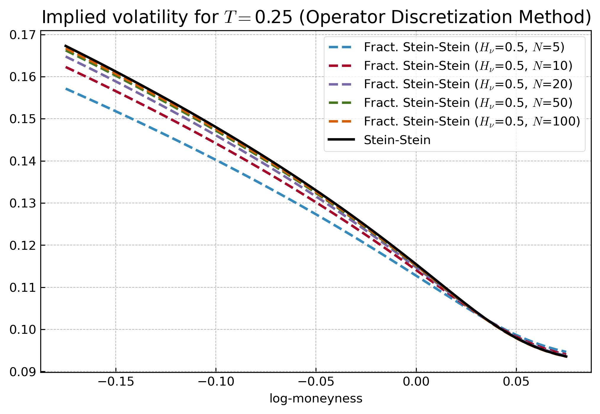
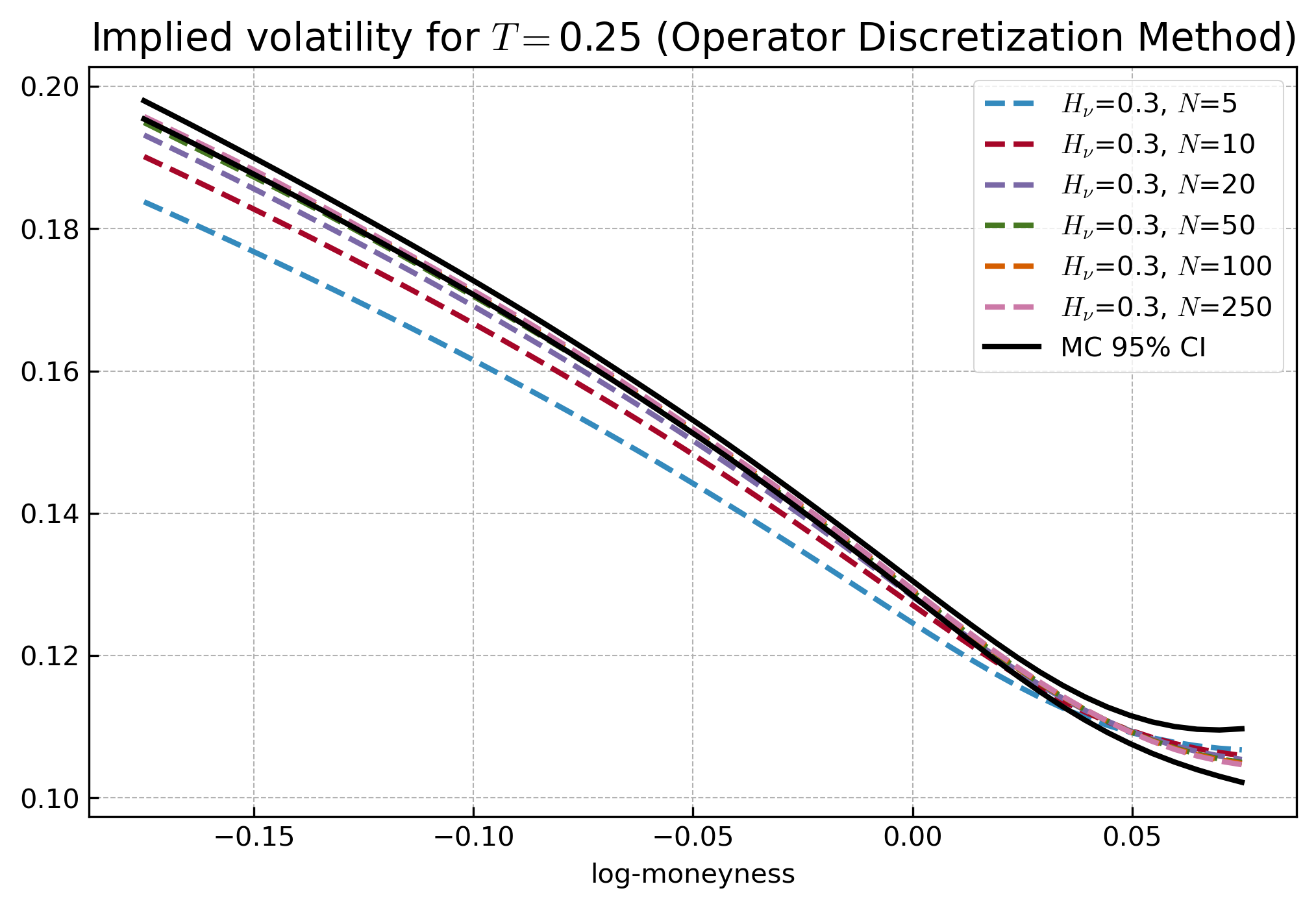
Figure 1: Implied volatility dynamics generated by the operator discretization method with $H_{\nu}=0.5$ and the Stein-Stein model (left); Implied volatility dynamics generated by the operator discretization method with $H_{\nu}=0.3$ (right). Monte Carlo confidence intervals are generated with $200\>000$ simulations of risk processes using a Euler scheme with $1/365$ as time-step.

4 Calibration to market data

In this section, we highlight the relevance of our framework for calibration on market data. To this end, we place ourselves in an equity market context where the process $(I_{t})_{0\leq t\leq T}$ represents an equity stock index. Our calibration instruments from market data, are interest rate options, caps and floors, as well as equity vanilla call and put options. Let us now calibrate the models to the market data in order to validate the relevance of the introduced framework. To this end, we consider market data of 25/08/2022 consisting of USD 3M Libor yield curve and ATM USD cap implied volatility data from Bloomberg, and S&P500 implied volatility data purchased from the CBOE website. The calibration procedure takes place in two stages. First we calibrate the interest rate parameters using the USD 3M Libor yield curve and ATM cap data. Then, using these calibrated interest rate parameters, we calibrate the volatility and correlation parameters based on S&P500 implied volatility data.

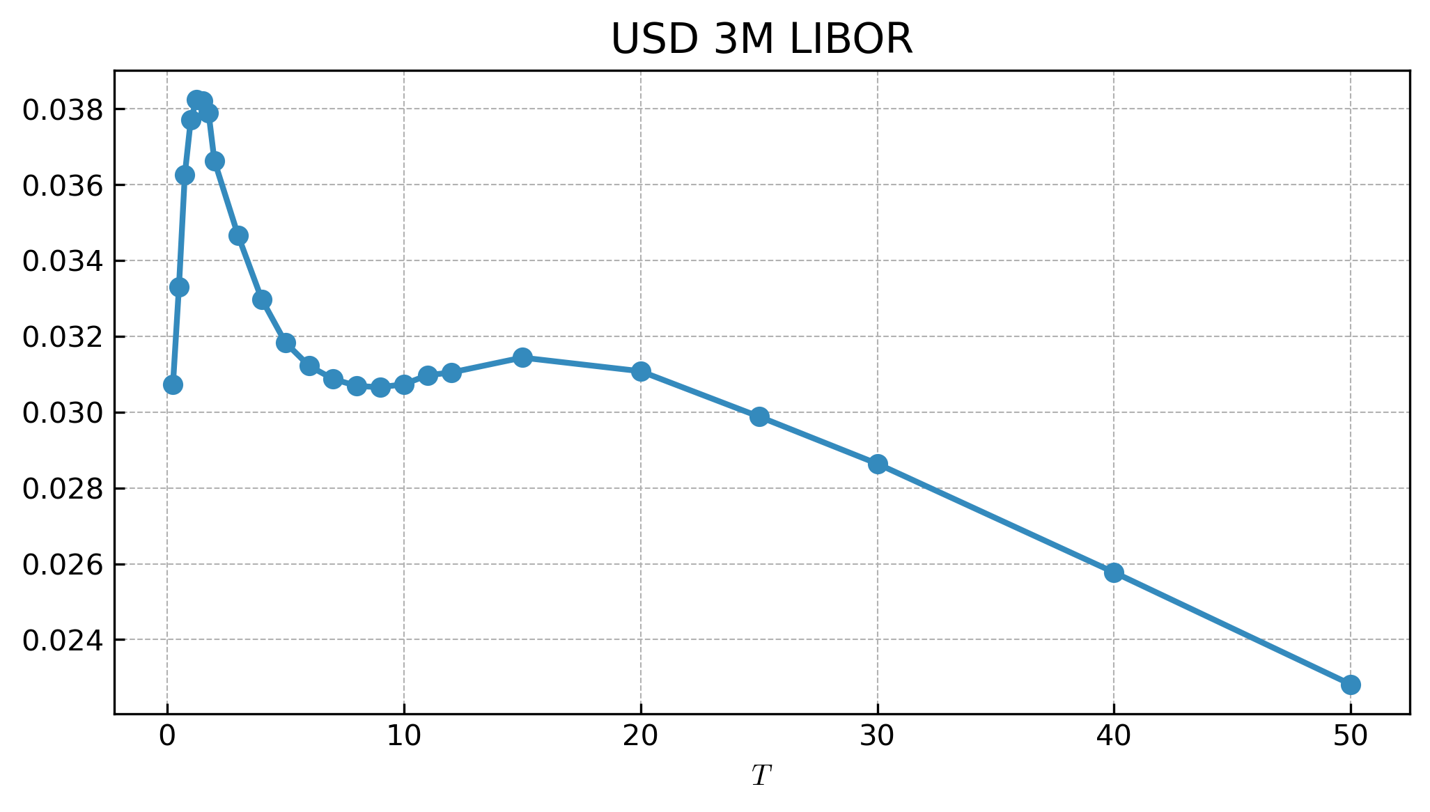
Figure 2: USD 3M Libor yield curve of 25/08/2022.

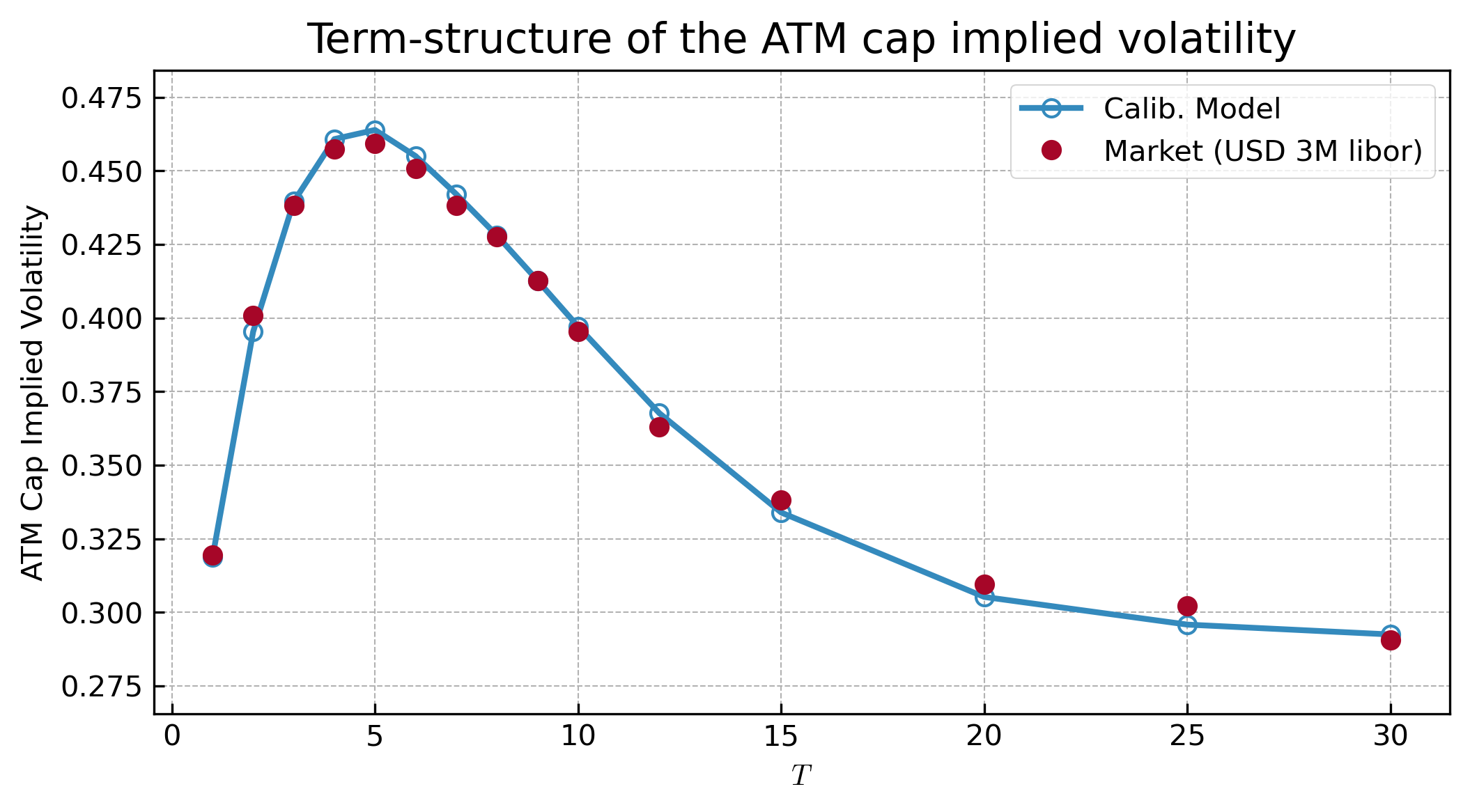
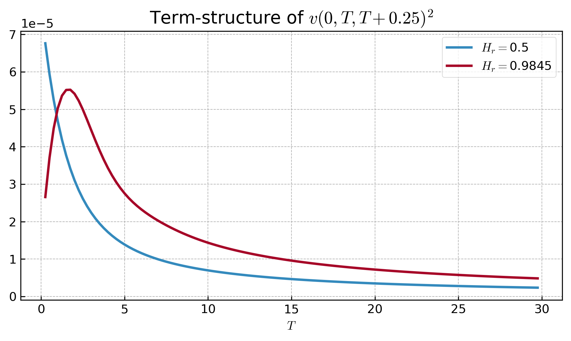
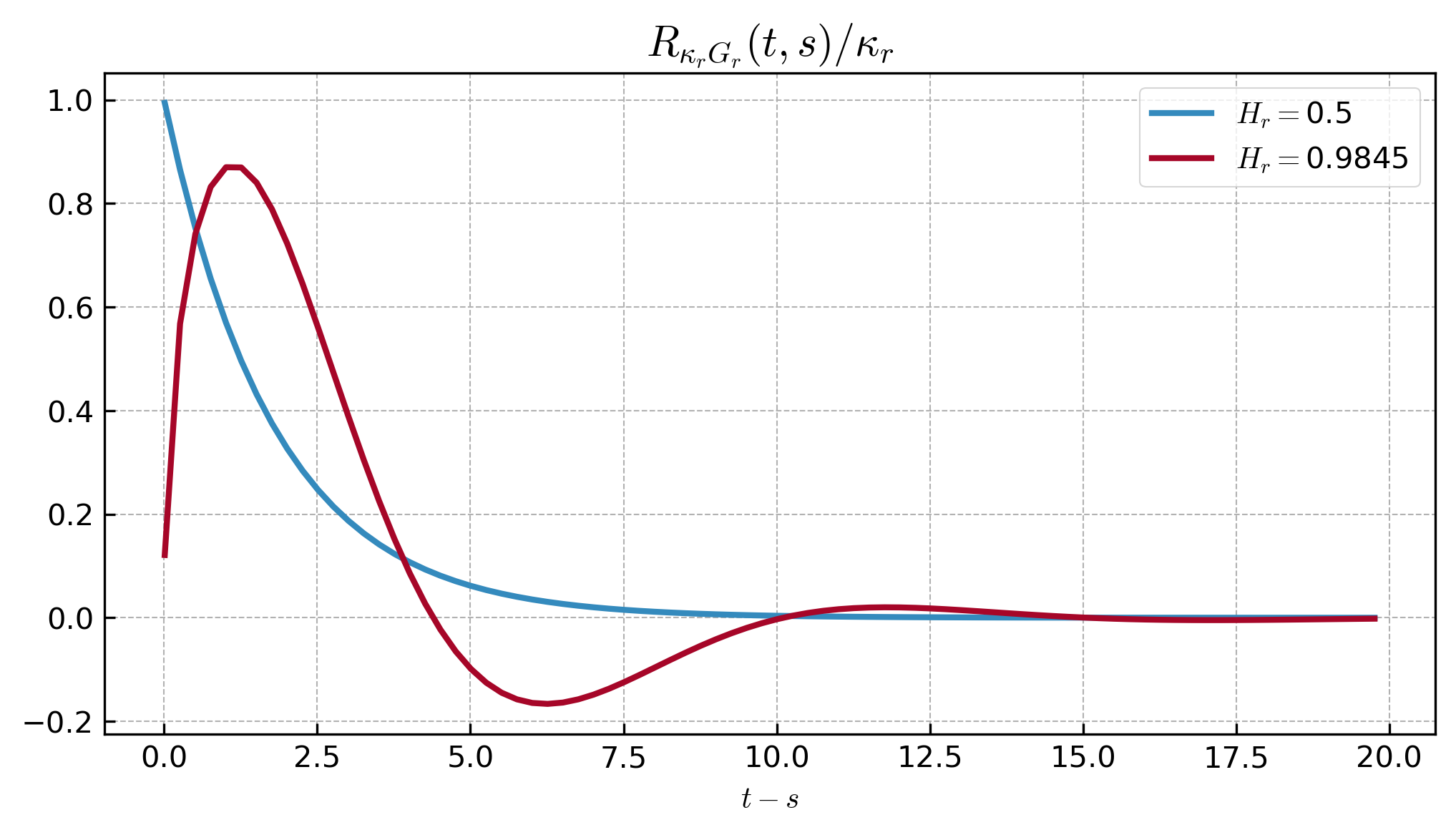
Figure 3: ATM cap implied volatility for USD 3M Libor: calibrated fractional model vs market data of 25/08/2022. RMSE: 0.3663%. Calibrated parameters: $\hat{\kappa}_{r}=-0.5566,$ $\hat{\eta}_{r}=0.0377$ and $\hat{H}_{r}=0.9845$ (top); term-structure of the ZC bond option pricing variance (2.10) generated with the calibrated parameters (bottom left); evolution of the resolvent associated to fractional kernel (bottom right).

For the interest model, we consider the fractional kernel of the form $G_{r}(t,s)=1_{s<t}\frac{(t-s)^{H_{r}-1/2}}{\Gamma(H_{r}+1/2)}.$ The data we have for the calibration are the USD 3M Libor yield curve and the ATM USD cap implied volatility for annual maturities ranging from 1 year to 30 years. Firstly, using (2.7) and the USD 3M Libor yield curve (Figure 2), the input curve $r_{0}(t)$ can deduced such that $P(0,T)=P^{Market}(0,T).$ Then, since cap options are sum of zero-coupon bond options, we use Proposition 2.2 and calibrate the interest rate parameters by minimizing the root square error (RMSE) between model and market ATM cap implied volatility. Results of this calibration are displayed on Figure 3 with the corresponding calibrated parameters. The RMSE is 0.3663% and we observe an excellent fit of the data with $\hat{H}_{r}>1/2$ as the calibrated model perfectly reproduces the humped shape of the market ATM cap implied volatility term-structure with only three parameters. As revealed by Figure 3, this can be explained by the fact that the term-structure of the ZC bond options pricing variance (2.10), with $S=T+1/4,$ produces a humped shape when $\kappa_{r}<0$ and $H_{r}>1/2$, which is totally not the case when considering the Hull-White model (i.e. $H_{r}=1/2)$. Moreover, as expected and revealed in Figure 4, $H_{r}>1/2$ generates a smoother sample path than $H_{r}=1/2$, and exhibits long-range dependencies. To check that long-term dependence makes sense, we consider historical data on the USD 3M Libor rate (daily close values) from 01/06/2021 to 30/09/2024, and examine the empirical auto-correlation structure. As we can see in Figure 4, the USD rate exhibits strong persistence, which is perfectly in line with previous studies (see Dai and Singleton (2003); McCarthy et al. (2004)), and emphasizes that considering long-range dependence models seems appropriate for modeling the dynamics of short rates.

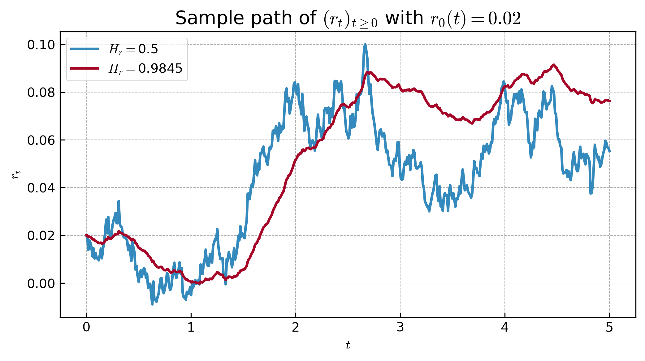
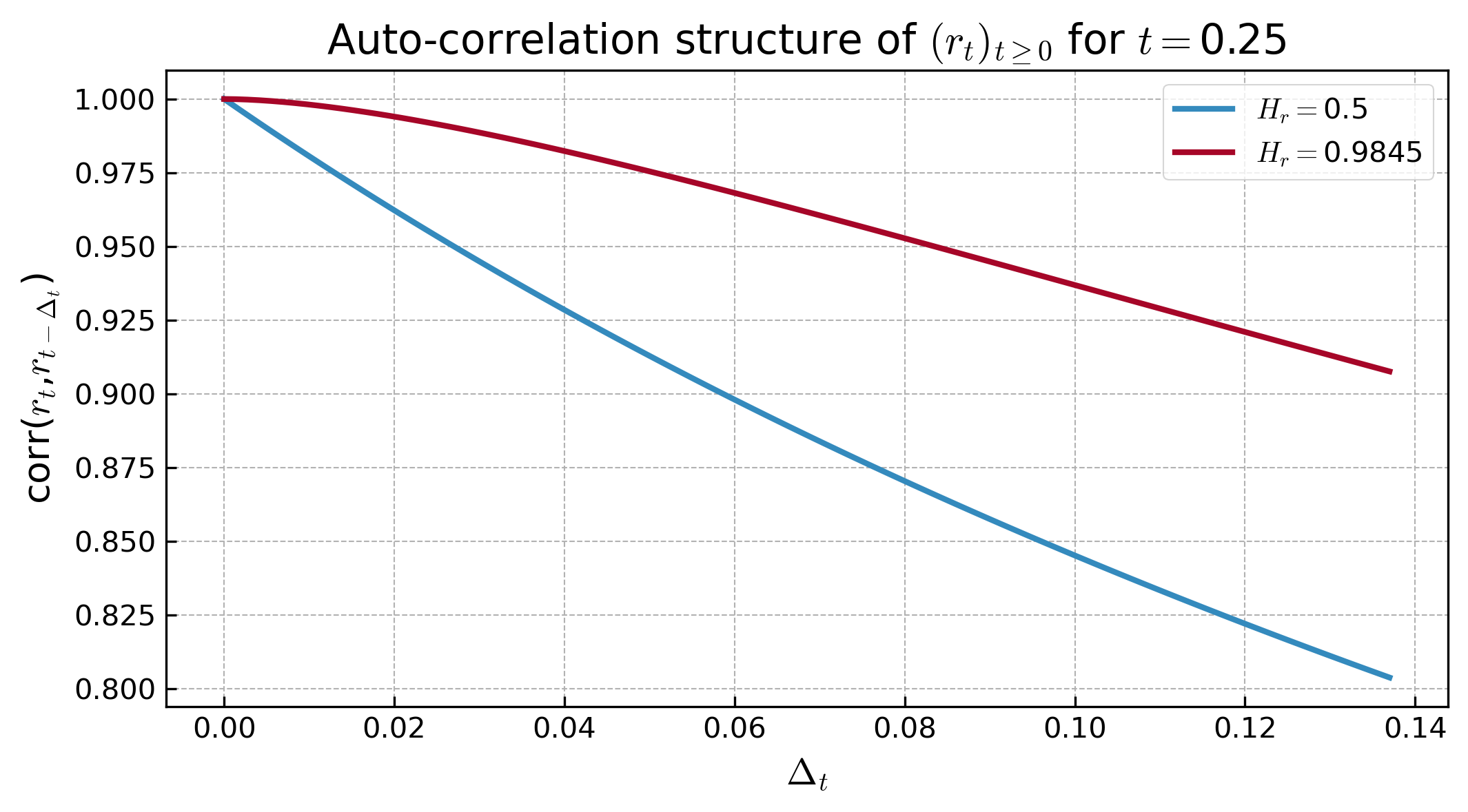
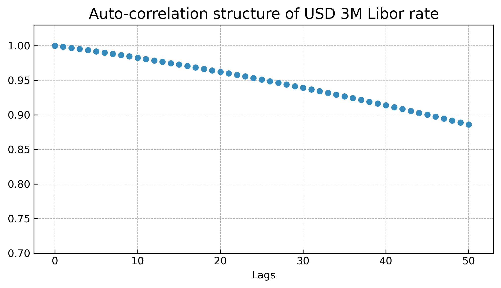
Figure 4: Sample path of $(r_{t})_{t\geq 0}$ generated with the calibrated parameters (upper left); Theoretical auto-correlation structure of $(r_{t})_{t\geq 0}$ with the calibrated parameters (upper right); Empirical auto-correlation structure of USD 3M Libor rates (bottom).

Let us now consider the calibration of the volatility and correlation parameters. To this end, we consider the fractional kernel of the form $G_{\nu}(t,s)=1_{s<t}\frac{(t-s)^{H_{\nu}-1/2}}{\Gamma(H_{\nu}+1/2)}$ as well as the shifted fractional kernel of the form $G_{\nu}(t,s)=1_{s<t}\frac{(t-s+\varepsilon)^{H_{\nu}-1/2}}{\Gamma(H_{\nu}+1/2)},$ with $\varepsilon=1/52.$ The data we have for the calibration are the S&P500 implied volatility data for different maturities ranging from 1 week to 1.82 years and different strikes. Using the operator discretization method with $N=40$ to approximate the characteristic function of the log-forward index and a Fourier method, we can price efficiently call options. Therefore, we calibrate the volatility and correlation parameters by minimizing the RMSE between model and S&P500 implied volatility. To have a more parsimonious model, we decide to fix $\kappa_{\nu}=0$ and $\rho_{r\nu}=0$. We prefer to capture the correlation between the index and the interest rate $\rho_{Ir}$ rather than the correlation $\rho_{r\nu}$, but we have a leverage of flexibility if we decide to calibrate $\rho_{r\nu}$ as well.

Results of this calibration are displayed on Figure 5, 6 and 7, we observe that, for both kernels, $\hat{H}_{\nu}<1/2$. The RMSE are 0.4912% for the fractional kernel and 0.4204% for the shifted fractional kernel. Overall, the calibration is good for both kernels, especially around the ATM, yet the shifted fractional kernel outperforms the fractional kernel. Moreover, as we can observe on Figure 8, the shifted fractional kernel reproduces the term-structure of the ATM skew with a concave shape on the log-log scale for the chosen date, which is less the case for the fractional kernel. We observe that $\hat{H}_{\nu}^{\text{Shifted fractional}}<\hat{H}_{\nu}^{\text{Fractional}}$, indicating that the shifted kernel exhibits a faster decrease for longer maturities while $\varepsilon=1/52$ prevents it from having an exploding skew for shorter maturities, allowing it to better capture the concave shape of the skew (in log-log scale). Our results demonstrate that the rough model underperforms the non-rough model associated with the shifted fractional kernel in capturing the entire volatility surface, confirming the findings of Abi Jaber and Li (2024); Delemotte, De Marco, and Segonne (2023); Guyon and Lekeufack (2023).

We also observe that the calibrated correlations between interest rate and index processes $\hat{\rho}_{Ir}$ are significant. To ensure that these estimated values make sense, we looked at the empirical 180 days rolling correlation between the S&P500 index and the USD 3M Libor rate (daily close values). The results are displayed on Figure 9. We first observe that the correlation is not constant and almost never zero. Secondly, we notice that, for the calibration date we have chosen, the empirical rolling correlation is negative. This seems in line with the correlation values obtained during calibration on the implied volatility surface of the S&P500, and thus assuming correlation between processes appears coherent with market data.

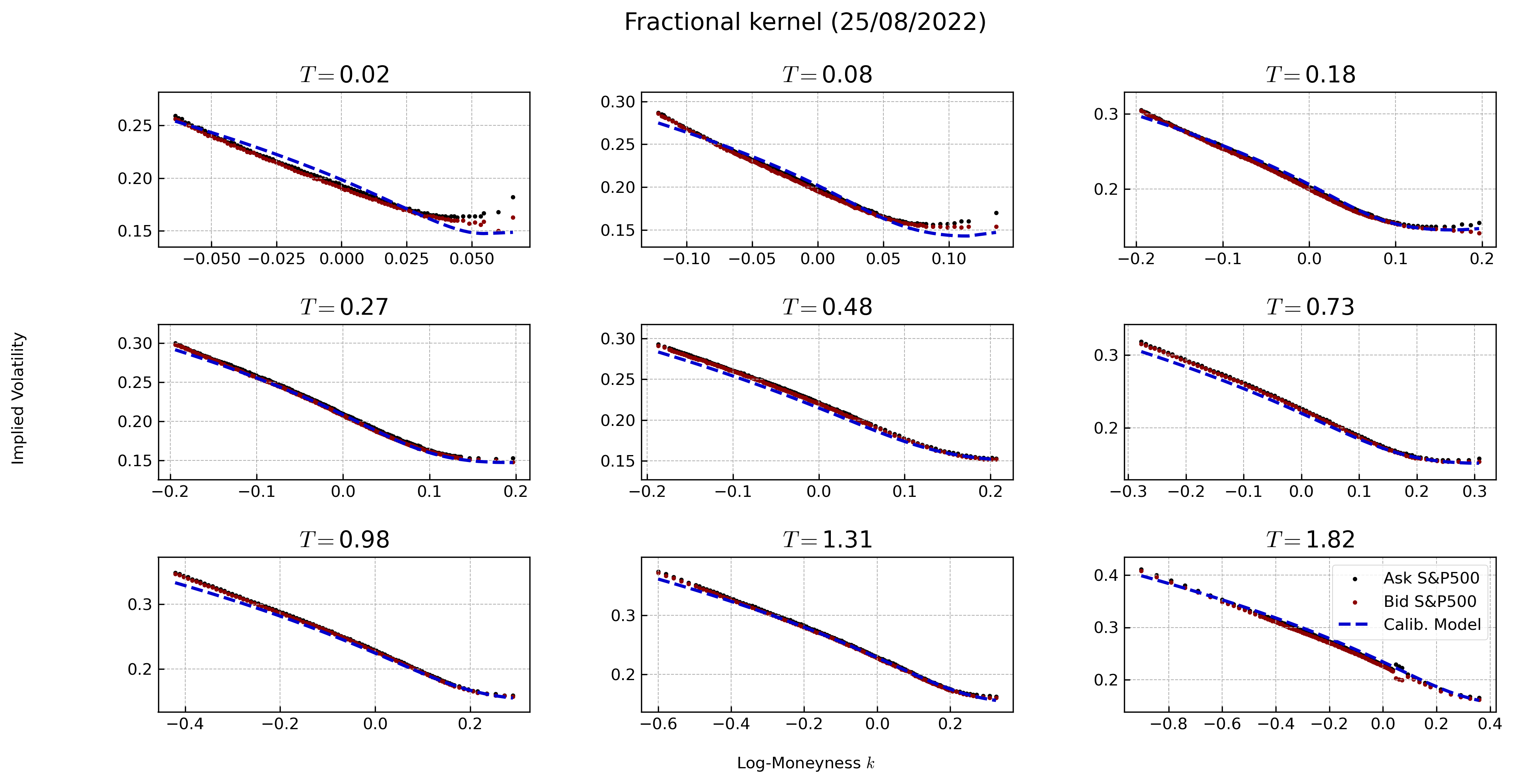
Figure 5: S&P500 implied volatility: calibrated fractional model vs market data of 25/08/2022. RMSE: 0.4912%. Calibrated parameters: $\hat{\nu}_{0}=0.1955$, $\hat{\theta}_{\nu}=-0.01909,$ $\hat{\eta}_{\nu}=0.2136,$ $\hat{\rho}_{I\nu}=-0.7916,$ $\hat{\rho}_{Ir}=-0.9613$ and $\hat{H}_{\nu}=0.3087$.

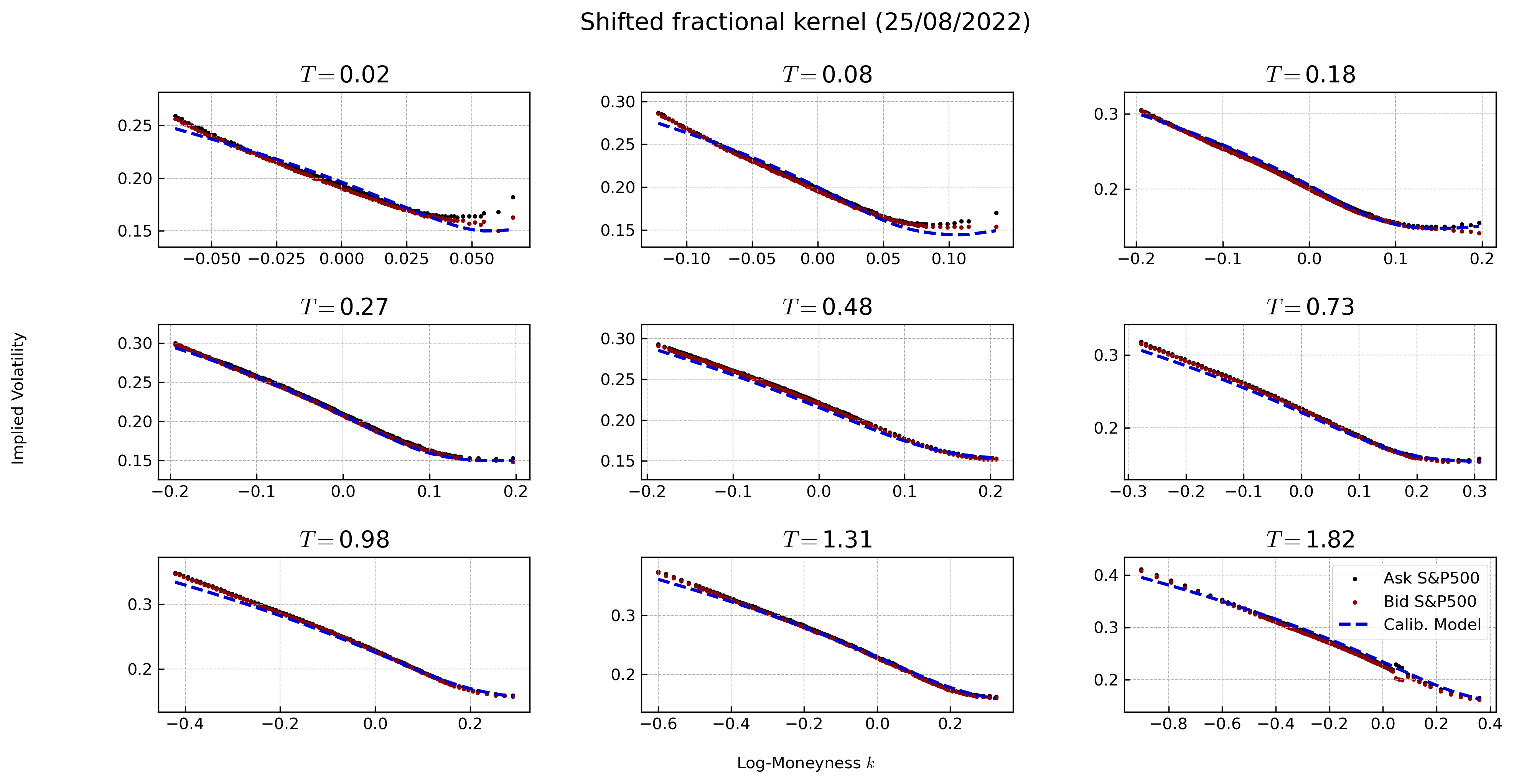
Figure 6: S&P500 implied volatility: calibrated shifted fractional model vs market data of 25/08/2022. RMSE: 0.4204%. Calibrated parameters: $\hat{\nu}_{0}=0.1960$, $\hat{\theta}_{\nu}=-0.0235,$ $\hat{\eta}_{\nu}=0.2194,$ $\hat{\rho}_{I\nu}=-0.7783,$ $\hat{\rho}_{Ir}=-0.9715$ and $\hat{H}_{\nu}=0.2229$.

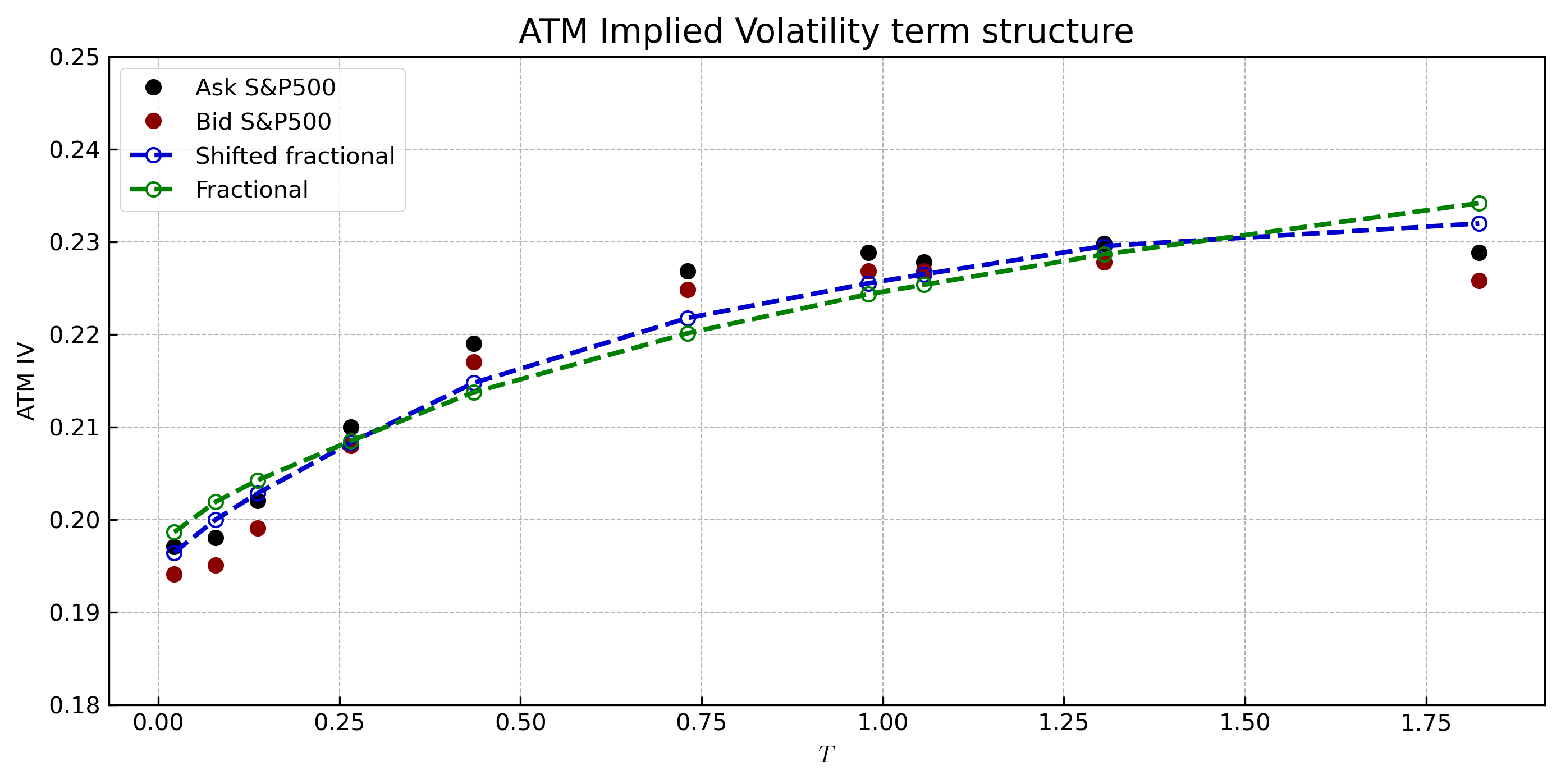
Figure 7: ATM implied volatility term structure: calibrated models vs market data of 25/08/2022 with calibrated parameters.

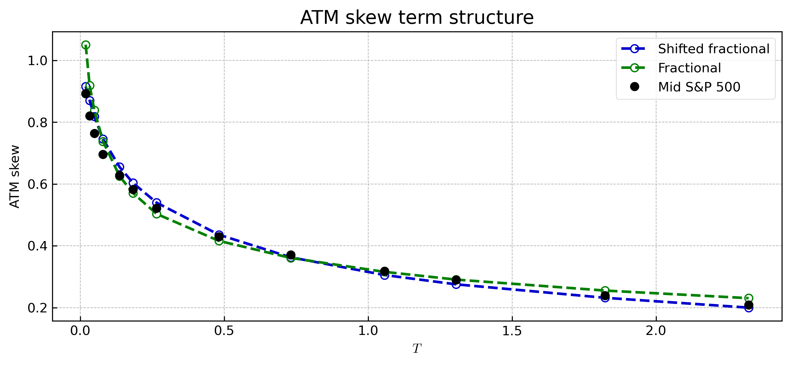
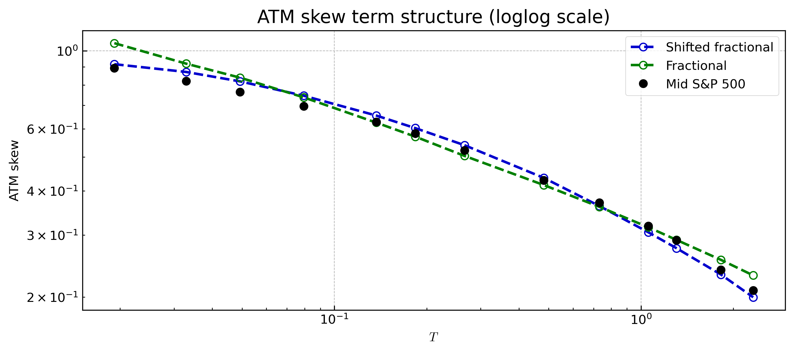
Figure 8: ATM skew term structure: calibrated models vs market data of 25/08/2022 with calibrated parameters.

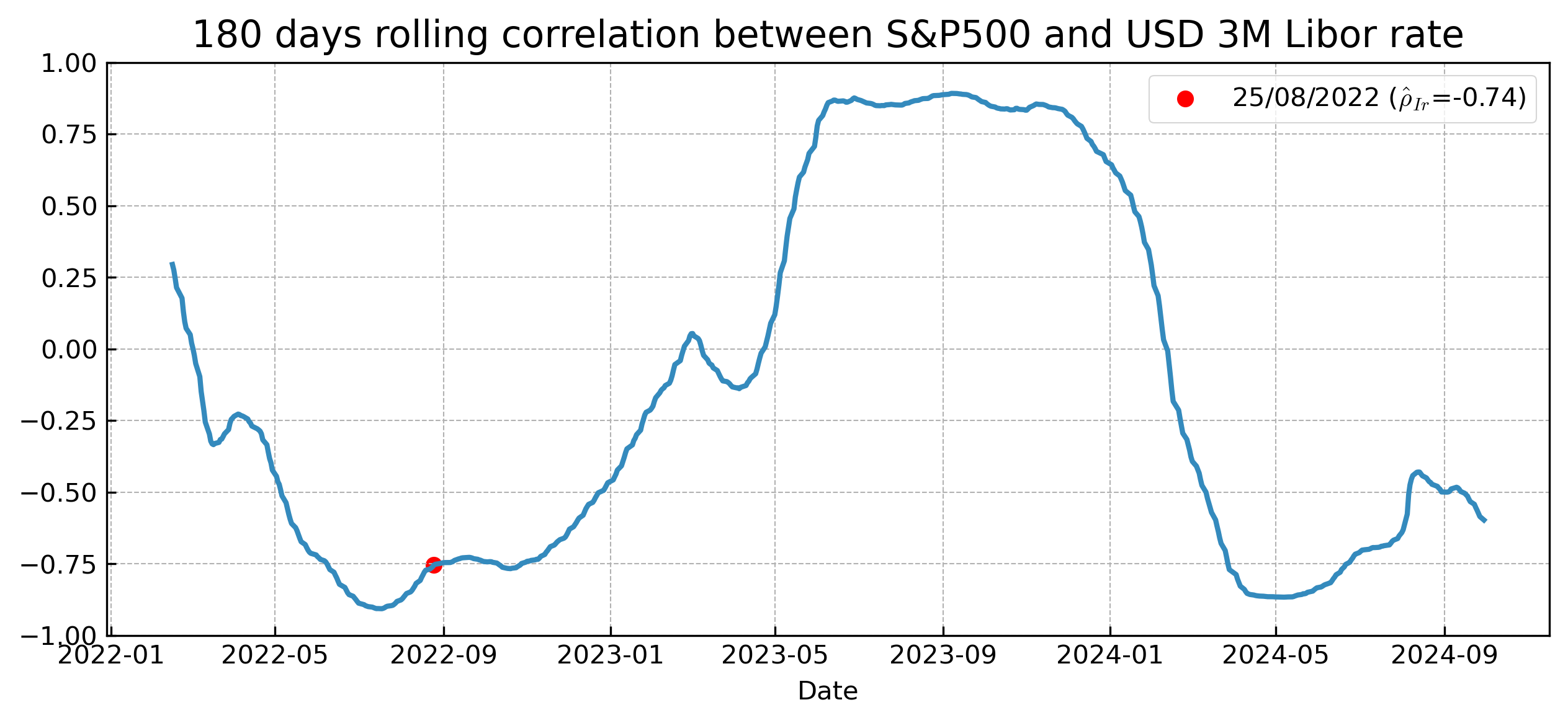
Figure 9: 180 days rolling correlation between S&P500 and USD 3M Libor rate.

5 Link with conventional quadratic linear models

5.1 Link with operator Riccati equations

In this section, we provide the link between the analytic expression of the characteristic function (3.2) and expression that depends on Riccati equations.

Proposition 5.1.

Let $g_{0}(.)$ be given by (2.3), $G_{\nu}(.)$ a Volterra kernel as in Definition 2.1. Fix $u\in\mathbb{C}$ such that $0\leq\mathcal{\mathfrak{R}}(u)\leq 1.$ Then, for all $t\leq T$,

$$E^{\mathbb{Q}^{T}}\bigg{[}\exp\bigg{(}u\log\frac{I_{T}^{T}}{I_{t}^{T}}\bigg{)}\bigg{|}\mathcal{F}_{t}\bigg{]}=\exp\left(\phi_{t}^{u}+\chi_{t}^{u}+a^{u}\int_{t}^{T}h_{t}^{u}(s)^{2}ds+\int_{t}^{T}\int_{t}^{T}h_{t}^{u}(s)h_{t}^{u}(w)\>\bar{\psi}_{t}^{u}(s,w)dsdw\right),$$ (5.1)

with $\chi_{t}^{u}$ as in Theorem 3.1, $\phi_{t}^{u}$ such that

$$\dot{\phi}_{t}^{u} =-a^{u}\eta_{\nu}^{2}\int_{t}^{T}G_{\nu}(s,t)^{2}ds-\eta_{\nu}^{2}\int_{t}^{T}\int_{t}^{T}G_{\nu}(s,t)G_{\nu}(w,t)\>\bar{\psi}_{t}^{u}(s,w)\,ds\,dw,\>t<T,$$

$$\phi_{T}^{u} =0,$$ (5.2)

and $\bar{\psi}_{t}^{u}(s,w)$ that satisfies a Riccati equation of the form

$$\dot{\bar{\psi}}_{t}^{u}(s,w)= 2(a^{u})^{2}\eta_{\nu}^{2}\,G_{\nu}(s,t)G_{\nu}(w,t)+2a^{u}\eta_{\nu}^{2}\bigg{(}G_{\nu}(s,t)\,(\mathbf{G}_{\nu}^{*}\bar{\psi}_{t}^{u}(.,w))(t)+G_{\nu}(w,t)\,(\mathbf{G}_{\nu}^{*}\bar{\psi}_{t}^{u}(s,.))(t)\bigg{)}$$

$$+2\eta_{\nu}^{2}\,(\mathbf{G}_{\nu}^{*}\bar{\psi}_{t}^{u}(s,.))(t)\>(\mathbf{G}_{\nu}^{*}\bar{\psi}_{t}^{u}(.,w))(t),\>t<T,\>(s,w)\in(t,T]^{2}\>a.e.,$$

$$\bar{\psi}_{t}(t,s)= \bar{\psi}_{t}(s,t)=b^{u}\bigg{(}a^{u}G_{\nu}(s,t)+(\mathbf{G}_{\nu}^{*}\bar{\psi}_{t}^{u}(s,.))(t)\bigg{)},\>t\leq s\leq T.$$

Proof.

From Lemma 6.1, we have that $\mathbf{\Psi}_{t}^{u}=a^{u}\text{id}+\bar{\mathbf{\Psi}}_{t}^{u}$, where $\bar{\mathbf{\Psi}}_{t}^{u}$ is an integral operator induced by a symmetric kernel $\bar{\psi}_{t}^{u}(s,w)$ such that

$$\bar{\psi}_{t}^{u}(t,s)=\bar{\psi}_{t}^{u}(s,t) =b^{u}\int_{t}^{T}G_{\nu}(w,t)(a^{u}\delta_{w=s}+\bar{\psi}_{t}^{u}(s,w))dw,\>t\leq s\leq T$$

$$=b^{u}\bigg{(}a^{u}G_{\nu}(s,t)+(\mathbf{G}_{\nu}^{*}\bar{\psi}_{t}^{u}(s,.))(t)\bigg{)},\>t\leq s\leq T.$$

In this case, we have that

$$\langle h_{t}^{u},\mathbf{\Psi}_{t}^{u}h_{t}^{u}\rangle_{L^{2}}=a^{u}\int_{t}^{T}h_{t}^{u}(s)^{2}\>ds+\int_{t}^{T}\int_{t}^{T}h_{t}^{u}(s)h_{t}^{u}(w)\>\bar{\psi}_{t}^{u}(s,w)\>dsdw.$$

Moreover, we also know from Lemma B.1. in Abi Jaber (2022a) that

$$\dot{\mathbf{\Psi}}_{t}^{u} =2\mathbf{\Psi}_{t}^{u}\dot{\mathbf{\Sigma}}_{t}\mathbf{\Psi}_{t}^{u},\>t<T,$$

$$\mathbf{\Psi}_{T}^{u} =a^{u}(\text{id}-b^{u}\mathbf{G}_{\nu}^{*})^{-1}(\text{id}-b^{u}\mathbf{G}_{\nu})^{-1},$$

and by the definition, we also have that

$$\dot{\bar{\mathbf{\Psi}}}_{t}^{u} =2\mathbf{\Psi}_{t}^{u}\dot{\mathbf{\Sigma}}_{t}\mathbf{\Psi}_{t}^{u},\>t<T,$$

$$=2(a^{u}\text{id}+\bar{\mathbf{\Psi}}_{t}^{u})\dot{\mathbf{\Sigma}}_{t}(a^{u}\text{id}+\bar{\mathbf{\Psi}}_{t}^{u}),\>t<T,$$

$$\bar{\mathbf{\Psi}}_{T}^{u} =a^{u}(\text{id}-b^{u}\mathbf{G}_{\nu}^{*})^{-1}(\text{id}-b^{u}\mathbf{G}_{\nu})^{-1}-a^{u}\text{id},$$

As $\dot{\bar{\mathbf{\Psi}}}_{t}^{u}$ is composed of integral operators, it is also an integral operator induced by the following kernel

$$2((a^{u}\delta+\bar{\mathbf{\Psi}}_{t}^{u})\star\dot{\mathbf{\Sigma}}_{t}\star(a^{u}\delta+\bar{\mathbf{\Psi}}_{t}^{u}))(s,w),$$

with $\delta$ the kernel induced by the identity operator such that $(\text{id}f)(s)=\int_{t}^{T}\delta_{s=w}(ds,dw)f(w)=f(s).$ Thus, using the dominated convergence theorem, we obtain that $t\to\bar{\psi}_{t}^{u}(s,w)$ solves a Riccati equation given, for $t<s$ and $w\leq T,$ by

$$\dot{\bar{\psi}}_{t}^{u}(s,w)=2((a^{u}\,\delta+\bar{\mathbf{\Psi}}_{t}^{u})\star\dot{\mathbf{\Sigma}}_{t}\star(a^{u}\,\delta+\bar{\mathbf{\Psi}}_{t}^{u}))(s,w).$$

More explicitly, since $G(z,t)=0$ for $z\leq t,$ we also have, for $(s,w)\in(t,T]^{2}\>a.e.$,

$$\dot{\bar{\psi}}_{t}^{u}(s,w)= 2(a^{u})^{2}\eta_{\nu}^{2}\,G_{\nu}(s,t)G_{\nu}(w,t)+2a^{u}\eta_{\nu}^{2}\,G_{\nu}(s,t)\int_{t}^{T}G_{\nu}(z,t)\,\bar{\psi}_{t}^{u}(z,w)\,dz$$

$$+2a^{u}\eta_{\nu}^{2}\,G_{\nu}(w,t)\int_{t}^{T}G_{\nu}(z,t)\,\bar{\psi}_{t}^{u}(s,z)\,dz$$

$$+2\eta_{\nu}^{2}\,\int_{t}^{T}G_{\nu}(z,t)\,\bar{\psi}_{t}^{u}(s,z)\,dz\int_{t}^{T}G_{\nu}(z^{{}^{\prime}},t)\,\bar{\psi}_{t}^{u}(z^{{}^{\prime}},w)\,dz^{{}^{\prime}},\>t<T.$$

Thus, using the integral operator $\mathbf{G}_{\nu}^{*},$ we obtain that, for $(s,w)\in(t,T]^{2}\>a.e.$,

$$\dot{\bar{\psi}}_{t}^{u}(s,w)= 2(a^{u})^{2}\eta_{\nu}^{2}\,G_{\nu}(s,t)G_{\nu}(w,t)+2a^{u}\eta_{\nu}^{2}\bigg{(}G_{\nu}(s,t)\,(\mathbf{G}_{\nu}^{*}\bar{\psi}_{t}^{u}(.,w))(t)+G_{\nu}(w,t)\,(\mathbf{G}_{\nu}^{*}\bar{\psi}_{t}^{u}(s,.))(t)\bigg{)}$$

$$+2\eta_{\nu}^{2}\,(\mathbf{G}_{\nu}^{*}\bar{\psi}_{t}^{u}(s,.))(t)\>(\mathbf{G}_{\nu}^{*}\bar{\psi}_{t}^{u}(.,w))(t),\>t<T.$$

In addition, from Theorem 3.1, we know that $t\to\phi_{t}^{u}$ satisfies the following ODE

$$\dot{\phi}_{t}^{u} =\text{Tr}(\mathbf{\Psi}_{t}^{u}\dot{\mathbf{\Sigma}_{t}}),\>t<T$$

$$=\text{Tr}((a^{u}\text{id}+\bar{\mathbf{\Psi}}_{t}^{u})\dot{\mathbf{\Sigma}_{t}}),\>t<T$$

$$=a^{u}\text{Tr}(\dot{\mathbf{\Sigma}_{t}})+\text{Tr}(\bar{\mathbf{\Psi}}_{t}^{u}\dot{\mathbf{\Sigma}_{t}}),\>t<T$$

$$=-a^{u}\eta_{\nu}^{2}\int_{t}^{T}G_{\nu}(s,t)^{2}ds-\eta_{\nu}^{2}\int_{t}^{T}\int_{t}^{T}G_{\nu}(s,t)G_{\nu}(w,t)\>\bar{\psi}_{t}^{u}(s,w)\,ds\,dw,\>t<T,$$

with $\phi_{T}^{u}=0.$ ∎

We go now a step further and deduce more explicit Riccati equations by considering completely monotone Volterra kernels.

Definition 5.1.

A kernel $G:[0,T]^{2}\to\mathbb{R}$ is a completely monotone Volterra kernel if it satisfies Definition 2.1 and admits a Laplace representation of the form

$$G(t,s)=1_{s<t}\int_{\mathbb{R}^{+}}e^{-(t-s)x}\lambda(dx),$$ (5.3)

where $\lambda(.)$ is a positive measure.

Proposition 5.2.

Assume that the kernel function $G_{\nu}(t,s)$ is completely monotone and can be represented as (5.3). Moreover, assume that $g_{0}(.)$ is given by (2.3) and that the kernel satisfies Definition 2.1. Fix $u\in\mathbb{C}$ such that $0\leq\mathcal{\mathfrak{R}}(u)\leq 1.$ Then, for all $t\leq T$,

$$E^{\mathbb{Q}^{T}}\bigg{[}\exp\bigg{(}u\log\frac{I_{T}^{T}}{I_{t}^{T}}\bigg{)}\bigg{|}\mathcal{F}_{t}\bigg{]}=\exp\bigg{(}\Theta_{t}^{u}+2\int_{\mathbb{R}_{+}}\Lambda_{t}^{u}(x)Y_{t}(x)\>\lambda(dx)+\int_{\mathbb{R}_{+}^{2}}\Gamma_{t}^{u}(x,y)Y_{t}(x)Y_{t}(y)\>\lambda(dx)\>\lambda(dy)\bigg{)},$$ (5.4)

where $t\to(\Theta_{t}^{u},\Lambda_{t}^{u},\Gamma_{t}^{u})$ solve Riccati equations of the form

$$\dot{\Theta}_{t}^{u}= \dot{\chi}_{t}^{u}-a^{u}\bigg{(}g_{0}^{T}(t)+\rho_{Ir}\eta_{r}B_{G_{r}}(t,T)\bigg{)}^{2}-\eta_{\nu}^{2}\bigg{(}2\bigg{(}\int_{\mathbb{R}_{+}}\Lambda_{t}^{u}(x)\>\lambda(dx))\bigg{)}^{2}+\int_{\mathbb{R}_{+}}\int_{\mathbb{R}_{+}}\Gamma_{t}^{u}(x,y)\>\lambda(dx)\>\lambda(dy)\bigg{)}$$

$$-2\int_{\mathbb{R}_{+}}\bigg{(}b^{u}g_{0}^{T}(t)+u\eta_{\nu}\rho_{\nu r}\eta_{r}B_{G_{r}}(t,T)\bigg{)}\>\Lambda_{t}^{u}(x^{{}^{\prime}})\>\lambda(dx^{\prime}),\>t<T,$$ (5.5)

$$\dot{\Lambda}_{t}^{u}(x)= -a^{u}\bigg{(}g_{0}^{T}(t)+\rho_{Ir}\eta_{r}B_{G_{r}}(t,T)\bigg{)}+x\Lambda_{t}^{u}(x)-2\eta_{\nu}^{2}\bigg{(}\int_{\mathbb{R}_{+}}\Gamma_{t}^{u}(x,x^{\prime})\>\lambda(dx^{\prime})\bigg{)}\bigg{(}\int_{\mathbb{R}_{+}}\Lambda_{t}^{u}(y)\>\lambda(dy)\bigg{)}$$

$$-\int_{\mathbb{R}_{+}}\bigg{(}b^{u}g_{0}^{T}(t)+u\eta_{\nu}\rho_{\nu r}\eta_{r}B_{G_{r}}(t,T)\,\bigg{)}\Gamma_{t}^{u}(x,x^{{}^{\prime}})\>\lambda(dx^{\prime})$$

$$-b^{u}\int_{\mathbb{R}_{+}}\Lambda_{t}^{u}(x^{{}^{\prime}})\>\lambda(dx^{\prime}),\>t<T,\>x\in\mathbb{R}_{+},$$ (5.6)

and

$$\dot{\Gamma}_{t}^{u}(x,y)= (x+y)\Gamma_{t}^{u}(x,y)-a^{u}-2\,\eta_{\nu}^{2}\bigg{(}\int_{\mathbb{R}_{+}}\Gamma_{t}^{u}(x,x^{\prime})\>\lambda(dx^{\prime})\bigg{)}\bigg{(}\int_{\mathbb{R}_{+}}\Gamma_{t}^{u}(y,y^{\prime})\>\lambda(dy^{\prime})\bigg{)}$$

$$-b^{u}\bigg{(}\int_{\mathbb{R}_{+}}\Gamma_{t}^{u}(x,x^{{}^{\prime}})\>\lambda(dx^{\prime})+\int_{\mathbb{R}_{+}}\Gamma_{t}^{u}(y^{{}^{\prime}},y)\>\lambda(dy^{\prime})\bigg{)},\>t<T,\>(x,y)\in\mathbb{R}_{+}^{2},$$ (5.7)

with $\Theta_{T}^{u}=\Lambda_{T}^{u}=\Gamma_{T}^{u}=0.$

Proof.

The proof is given in Section 6. ∎

Remark 5.1.

A general result about the existence and the uniqueness of solutions to Riccati equations (5.5)-(5.6)-(5.7) is provided in Abi Jaber et al. (2021b). $\square$

5.2 Riccati equations for Markovian volatility models

In this section, we consider some particular completely monotone kernels associated to Markovian volatility models. For those models, we derive a simplified version of the characteristic function based on Riccati equations. In particular, for the indicator $G_{\nu}(t,s)=1_{s<t}$ and exponential $G_{\nu}(t,s)=1_{s<t}\alpha\exp(-\beta(t-s))$ kernels, we obtain closed form expressions similar to the characteristic functions deduced in van Haastrecht et al. (2009).

Proposition 5.3.

Suppose that $G_{\nu}(t,s)=1_{s<t}\sum_{i=1}^{N}w_{i}e^{-x_{i}(t-s)}$ and $g_{0}(t)=\nu_{0}+\theta_{\nu}\sum_{i=1}^{N}\int_{0}^{t}w_{i}\exp(-x_{i}(t-s))ds$ with $\nu_{0}>0$ and $\theta_{\nu}\in\mathbb{R}$, then, for $u\in\mathbb{C}$ such that $0\leq\mathcal{\mathfrak{R}}(u)\leq 1,$

$$E^{\mathbb{Q}^{T}}\bigg{[}\exp\bigg{(}u\log\frac{I_{T}^{T}}{I_{t}^{T}}\bigg{)}\bigg{|}\mathcal{F}_{t}\bigg{]}=\exp\left(A_{t}^{u;\,N}+2\sum_{i=1}^{N}B_{t}^{u;\,i}\>\nu_{t}^{i}+\sum_{i=1}^{N}\sum_{j=1}^{N}C_{t}^{u;\,ij}\>\nu_{t}^{i}\nu_{t}^{j}\right),$$ (5.8)

with $\left((\nu_{t}^{i})_{i=1,...,N}\right)_{0\leq t\leq T}$ solution of the following SDEs

$$d\nu_{t}^{i} =(-x_{i}\nu_{t}^{i}+\theta(t)+\kappa_{\nu}\>\nu_{t})\>dt+\eta_{\nu}\>dW_{\nu}^{\mathbb{Q}^{T}}(t),\>t>0,\>i=1,...,N,$$

$$\nu_{0}^{i} =0,$$

on $(\Omega,\mathcal{F},(\mathcal{F}_{t})_{t\leq T},\mathbb{Q}^{T})$ with $\theta(t):=\theta_{\nu}-\eta_{\nu}\sum_{i=1}^{n}\eta_{i}\rho_{i\nu}B_{i}(t,T)$, such that, almost surely,

$$\nu_{t}=\nu_{0}+\sum_{i=1}^{N}w_{i}\nu_{t}^{i},\>t\leq T,$$

and $A_{t}^{u;\,N}$, $(B_{t}^{u;\,i})_{i=1,...,N}$ and $(C_{t}^{u;\,ij})_{i,j=1,...,N}$ time-dependent functions satisfying Riccati equations of the form

$$\dot{A}_{t}^{u;\,N} =-a^{u}\bigg{(}\nu_{0}^{2}+\eta_{r}^{2}B_{G_{r}}(t,T)^{2}-2\nu_{0}\rho_{Ir}\eta_{r}B_{G_{r}}(t,T)\bigg{)}$$

$$-2\sum_{i=1}^{N}B_{t}^{u;\,i}\bigg{(}\theta(t)+u\eta_{\nu}\rho_{\nu r}\eta_{r}B_{G_{r}}(t,T)+b^{u}\nu_{0}\bigg{)}-\eta_{\nu}^{2}\sum_{i,j=1}^{N}(2B_{t}^{u;\,i}B_{t}^{u;\,j}+C_{t}^{u;\,ij}),\>t<T.$$ (5.9)

$$\dot{B}_{t}^{u;\,i}= x_{i}B_{t}^{u;\,i}-a^{u}w_{i}\bigg{(}\nu_{0}+\rho_{Ir}\eta_{r}B_{G_{r}}(t,T)\bigg{)}-2\eta_{\nu}^{2}\sum_{j,k=1}^{N}C_{t}^{u;\,ij}B_{t}^{u;\,k}$$

$$-w_{i}b^{u}\sum_{j=1}^{N}B_{t}^{u;\,j}-\sum_{j=1}^{N}C_{t}^{u;\,ij}\bigg{(}\theta(t)+u\eta_{\nu}\rho_{\nu r}\eta_{r}B_{G_{r}}(t,T)+b^{u}\nu_{0}\bigg{)},\>t<T,\>i=1,...,N,$$ (5.10)

$$\dot{C}_{t}^{u;\,ij}=(x_{i}+x_{j})C_{t}^{u;\,ij}-w_{i}w_{j}a^{u}-2\eta_{\nu}^{2}\sum_{k=1}^{N}\sum_{l=1}^{N}C_{t}^{u;\,ik}C_{t}^{u;\,jl}-b^{u}\sum_{k=1}^{N}\bigg{(}w_{j}C_{t}^{u;\,ik}+w_{i}C_{t}^{u;\,kj}\bigg{)}$$ (5.11)

with $A_{T}^{u;\,N}=B_{T}^{u;\,i}=C_{T}^{u;\,ij}=0,$ for $i,j=1,...,N.$

Proof.

The proof is given in Section 6. ∎

Corollary 5.1.

Suppose that $G_{\nu}(t,s)=1_{s<t}\>\alpha\exp(-\beta(t-s))$ and $g_{0}(t)=\nu_{0}+\theta_{\nu}\int_{0}^{t}\alpha\exp(-\beta(t-s))ds,$ with $\nu_{0}>0$, $\alpha,\beta\in\mathbb{R}_{+}$ and $\theta_{\nu}\in\mathbb{R}$. Then, for $u\in\mathbb{C}$ such that $0\leq\mathcal{\mathfrak{R}}(u)\leq 1,$

$$E^{\mathbb{Q}^{T}}\bigg{[}\exp\bigg{(}u\log\frac{I_{T}^{T}}{I_{t}^{T}}\bigg{)}\bigg{|}\mathcal{F}_{t}\bigg{]}=\exp(A_{t}^{u}+2B_{t}^{u}\>\nu_{t}+C_{t}^{u}\>\nu_{t}^{2}),$$ (5.12)

with $A_{t}^{u}$, $B_{t}^{u}$ and $C_{t}^{u}$ time-dependent functions given by

$$A_{t}^{u} =-\frac{1}{2}u(1-u)V_{r}(t,T)+\int_{t}^{T}\bigg{[}\bigg{(}\alpha\theta_{\nu}+(u-1)\rho_{\nu r}\alpha\eta_{\nu}\eta_{r}B_{G_{r}}(t,T)\bigg{)}B_{s}^{u}$$

$$\;\;\;\;\;\;\;\;\;\;\;\;\;\;\;\;\;\;+\frac{1}{2}\eta_{\nu}^{2}\bigg{(}(B_{s}^{u})^{2}+C_{s}^{u}\bigg{)}\bigg{]}\>ds,$$ (5.13)

$$B_{t}^{u} =-\frac{1}{2}\frac{u(1-u)}{\gamma_{1}+\gamma_{2}e^{-2\gamma(T-t)}}\bigg{[}\gamma_{0}(1+e^{-2\gamma(T-t)})$$

$$\;\;\;\;\;+(\gamma_{3}-\gamma_{4}e^{-2\gamma(T-t)}-(\gamma_{5}e^{-\kappa_{r}(T-t)}-\gamma_{6}e^{-(2\gamma+\kappa_{r})(T-t)})-\gamma_{7}e^{-\gamma(T-t)}\bigg{]},$$ (5.14)

$$C_{t}^{u}=-\frac{1}{2}u(1-u)\frac{1-e^{-2\gamma(T-t)}}{\gamma_{1}+\gamma_{2}e^{-2\gamma(T-t)}},$$ (5.15)

where $V_{r}(t,T)$ is the integrated variance of the interest rate process (2.1) and

$$\gamma =\sqrt{(-(\alpha\kappa_{\nu}-\beta)-\rho_{I\nu}\alpha\eta_{\nu}u)^{2}-\alpha^{2}\eta_{\nu}^{2}(u^{2}-u)},\>\>\>\>\>\>\gamma_{0}=\frac{\alpha\theta_{\nu}}{\gamma},$$

$$\gamma_{1} =\gamma-(\alpha\kappa_{\nu}-\beta+\rho_{I\nu}\alpha\eta_{\nu}u),\>\>\>\>\>\>\>\>\>\>\>\>\>\>\>\>\>\>\>\>\>\>\>\>\>\>\>\>\>\>\>\>\>\>\>\>\>\>\>\>\>\>\>\gamma_{2}=\gamma((\alpha\kappa_{\nu}-\beta+\rho_{I\nu}\alpha\eta_{\nu}u),$$

$$\gamma_{3} =\frac{\rho_{Ii}\eta_{r}\gamma_{1}+\rho_{\nu i}\eta_{r}\alpha\eta_{\nu}(u-1)}{\kappa_{r}\gamma},\>\>\>\>\>\>\>\>\>\>\>\>\>\>\>\>\>\>\>\>\>\>\>\>\>\>\>\>\>\>\>\>\>\>\>\>\>\>\>\>\gamma_{4}=\frac{\rho_{Ir}\eta_{r}\gamma_{2}-\rho_{\nu r}\eta_{r}\alpha\eta_{\nu}(u-1)}{\kappa_{r}\gamma},$$

$$\gamma_{5} =\frac{\rho_{Ir}\eta_{r}\gamma_{1}+\rho_{\nu r}\eta_{r}\alpha\eta_{\nu}(u-1)}{\kappa_{r}(\gamma-\kappa_{r})},\>\>\>\>\>\>\>\>\>\>\>\>\>\>\>\>\>\>\>\>\>\>\>\>\>\>\>\>\>\>\>\>\>\>\>\>\>\>\>\gamma_{6}=\frac{\rho_{Ir}\eta_{r}\gamma_{2}-\rho_{\nu r}\eta_{r}\alpha\eta_{\nu}(u-1)}{\kappa_{r}(\gamma+\kappa_{r})},$$

$$\gamma_{7} =(\gamma_{3}-\gamma_{4})-(\gamma_{5}-\gamma_{6}).$$

Proof.

Based on Proposition 5.3 with $N=1$, $w_{1}=1$ and $x_{1}=\alpha$, we deduce the Riccati equations satisfied by $A_{t}^{u},$$B_{t}^{u},$ $C_{t}^{u}$. Thus, using a laborious development as in van Haastrecht et al. (2009); van Haastrecht and Pelsser (2011), we can obtain the explicit forms given by (5.13)-(5.14)-(5.15). ∎

5.3 Multi-factor approximation for completely monotone Volterra kernels

In this section, we propose another alternative to approximate the characteristic function when considering completely monotone Volterra kernels in the sense of Definition 2.1. The approximate method is based on a Laplace representation of completely monotone kernels and expression of the characteristic function in terms of Riccati equations. Unlike the approach proposed in Section 3.2, a convergence result is deduced for this multi-factor approximate approach. Using a Laplace transform representation, we have that completely monotone kernels can be rewritten such that

$$G_{\nu}(t,s)=1_{s<t}\int_{\mathbb{R}^{+}}e^{-(t-s)x}\lambda(dx),$$ (5.16)

with $\lambda(.)$ a positive measure. Hence a natural approximation of the kernel is given by

$$\hat{G}_{\nu}(t,s):=1_{s<t}\sum_{i=1}^{N}\hat{w}_{i}e^{-(t-s)\hat{x}_{i}},$$ (5.17)

where $(\hat{w}_{i})_{i=1,...,N}$ are the weights and $(\hat{x}_{i})_{i=1,...,N}$ the mean reversion terms that should be appropriately defined. Under suitable choice, $\hat{G}_{\nu}$ converges in $L^{2}([0,T]^{2},\mathbb{R})$ to the completely monotone kernels. Therefore, based on Proposition 5.3, we can propose another approximate solution of the characteristic function associated to completely monotone Volterra kernels.

Lemma 5.1.

Suppose that for all $N\geq 1$, $(\hat{w}_{i})_{i=1,...,N}$ and $(\hat{x}_{i})_{i=1,...,N}$ are such that

$$\hat{w}_{i}:=\int_{k_{i-1}}^{k_{i}}\lambda(dk),\>\hat{x}_{i}:=\frac{1}{\hat{w}_{i}}\int_{k_{i-1}}^{k_{i}}k\;\lambda(dk),$$

such that $k_{0}=0<k_{1}<...<k_{n}$ and

$$k_{n}\to\infty,\>\sum_{i=1}^{N}\int_{k_{i-1}}^{k_{i}}(k_{i}-k)^{2}\;\lambda(dk)\to 0.$$

as $N$ goes to infinity. For $N\geq 1$ fixed, there exists a function $f_{N}^{(2)}((k_{i})_{i=0,...,N})$ such that the following inequality holds

$$||\hat{G}_{\nu}-G_{\nu}||_{L^{2}([0,T]^{2},\mathbb{R})}\leq f_{N}^{(2)}((k_{i})_{i=1,...,N}),$$ (5.18)

and $\hat{G}_{\nu}$ converges in $L^{2}([0,T]^{2},\mathbb{R})$ to $G_{\nu}$ when $N$ goes to infinity i.e.

$$||\hat{G}_{\nu}-G_{\nu}||_{L^{2}([0,T]^{2},\mathbb{R})}\to 0,$$

as $N$ goes to infinity.

Proof.

We refer to the proof of (Abi Jaber and El Euch, 2019, Proposition 3.3.). ∎

Remark 5.2.

As stated in Abi Jaber and El Euch (2019), there are different possible choices of the auxiliary terms $(k_{i})_{i=0,...,N}$. In this paper, for fixed $N\geq 1,$ we take auxiliary terms $(k_{i})_{i=0,...,N}$ that minimize the upper bound (5.18). Thus, we choose $(k_{i})_{i=1,...,N}$ solutions of

$$\inf_{(k_{i})_{i=1,..,N}\in\mathcal{E}_{N}}f_{N}^{(2)}((k_{i})_{i=1,...,N}),$$

with $\mathcal{E}_{N}:=\{(k_{i})_{i=1,..,N}:\;k_{0}=0<k_{1}<...<k_{n}\}.$

Proposition 5.4.

Let $(I_{t}^{T})_{0\leq t\leq T}$ be the solution of (2.12) with the completely monotone kernel (5.16) and $(\tilde{I}_{t}^{T})_{0\leq t\leq T}$ solution of (2.12) with the approximate kernel (5.17). Suppose that the assumptions of Lemma 5.1 are satisfied and that, for $u\in\mathbb{C}$ such that $0\leq\mathcal{\mathfrak{R}}(u)\leq 1,$ the sequence $(\exp(u\log\tilde{I}_{T}^{T}))_{N\in\mathbb{N}}$ is uniformly integrable, then

$$\lim_{N\to\infty}\exp(A_{0}^{u;\,N})=E^{\mathbb{Q}^{T}}\bigg{[}\exp\bigg{(}u\log\frac{I_{T}^{T}}{I_{0}^{T}}\bigg{)}\bigg{|}\mathcal{F}_{0}\bigg{]},$$

where $A_{0}^{u;\,N}$ is the solution of Riccati equation (5.9) with $w_{i}=\hat{w}_{i}$ and $x_{i}=\hat{x}_{i}$, for $i=1,...,N.$

Proof.

Using arguments similar to those of Motte and Hainaut (2024), we can show that, for $t\in[0,T],$

$$\tilde{I}_{t}^{T}\xrightarrow{\mathcal{L}}I_{t}^{T},$$

as $N$ goes to infinity, where $\xrightarrow{\mathcal{L}}$ stands for weak convergence. Therefore, using the uniform integrability of $\exp(u\log\tilde{I}_{T}^{T})$ and the fact that $I_{0}^{T}=\tilde{I}_{0}^{T},$ we obtain that

$$\lim_{N\to\infty}E^{\mathbb{Q}^{T}}\bigg{[}\exp\bigg{(}u\log\frac{\tilde{I}_{T}^{T}}{\tilde{I}_{0}^{T}}\bigg{)}\bigg{|}\mathcal{F}_{0}\bigg{]}=E^{\mathbb{Q}^{T}}\bigg{[}\exp\bigg{(}u\log\frac{I_{T}^{T}}{I_{0}^{T}}\bigg{)}\bigg{|}\mathcal{F}_{0}\bigg{]},$$

and thus, we conclude the proof using Corollary 5.3 and the fact that $\nu_{0}^{i}=0$ for $i=1,...,N.$ ∎

Based on Proposition 5.4, we can deduce a second approximate solution of the characteristic function for which a theoretical convergence result is established. However, it is a semi-closed solution in the sense that it requires solving Riccati equations.

Finally, we decide to compare this “multi-factor” approximate method with the “operator discretization” method proposed in Section 3.2. For this purpose, we consider the same kernels and model parameters as in Section 3.2. Figure 10 presents the implied volatility generated for different $N$ by the multi-factor method where the system of Riccati $(N^{2}+N+1)$ equations (5.9)-(5.10)-(5.11) is solved numerically using an implicit method. We observe a convergence as the number of factors increases. However, the speed of convergence differs between the methods. As revealed by Figure 11, the operator discretization approach converges much faster than the multi-factor approach, either with respect to $N$ or in terms of computation time. Nevertheless, it should be noted that the speed of convergence of the “multi-factor” method depends strongly on the choice of multi-factor parameters $(\hat{w}_{i},\hat{x}_{i})_{i=1,...,N}$ , as well as the numerical method used to solve the system of Riccati $(N^{2}+N+1)$ equations and other choices than those used in this paper could give a faster speed of convergence. The aim of this comparison is above all to illustrate that the “operator discretization” method converges quickly and is fairly simple to implement compared with the “multi-factor” method.

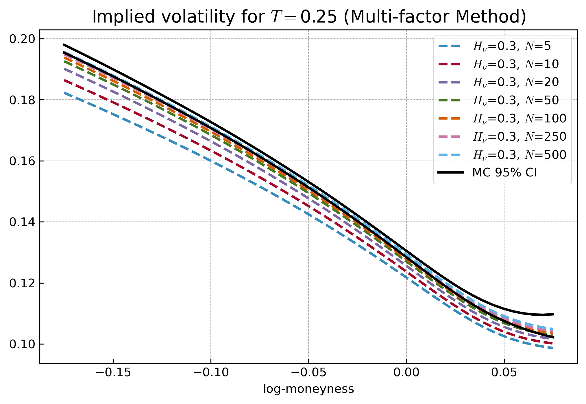
Figure 10: Implied volatility dynamics generated by the multi-factor approximation method with $H_{\nu}=0.3$ (right). Monte Carlo confidence intervals are generated with $200\>000$ simulations of risk processes using a Euler scheme with $1/365$ as time-step.

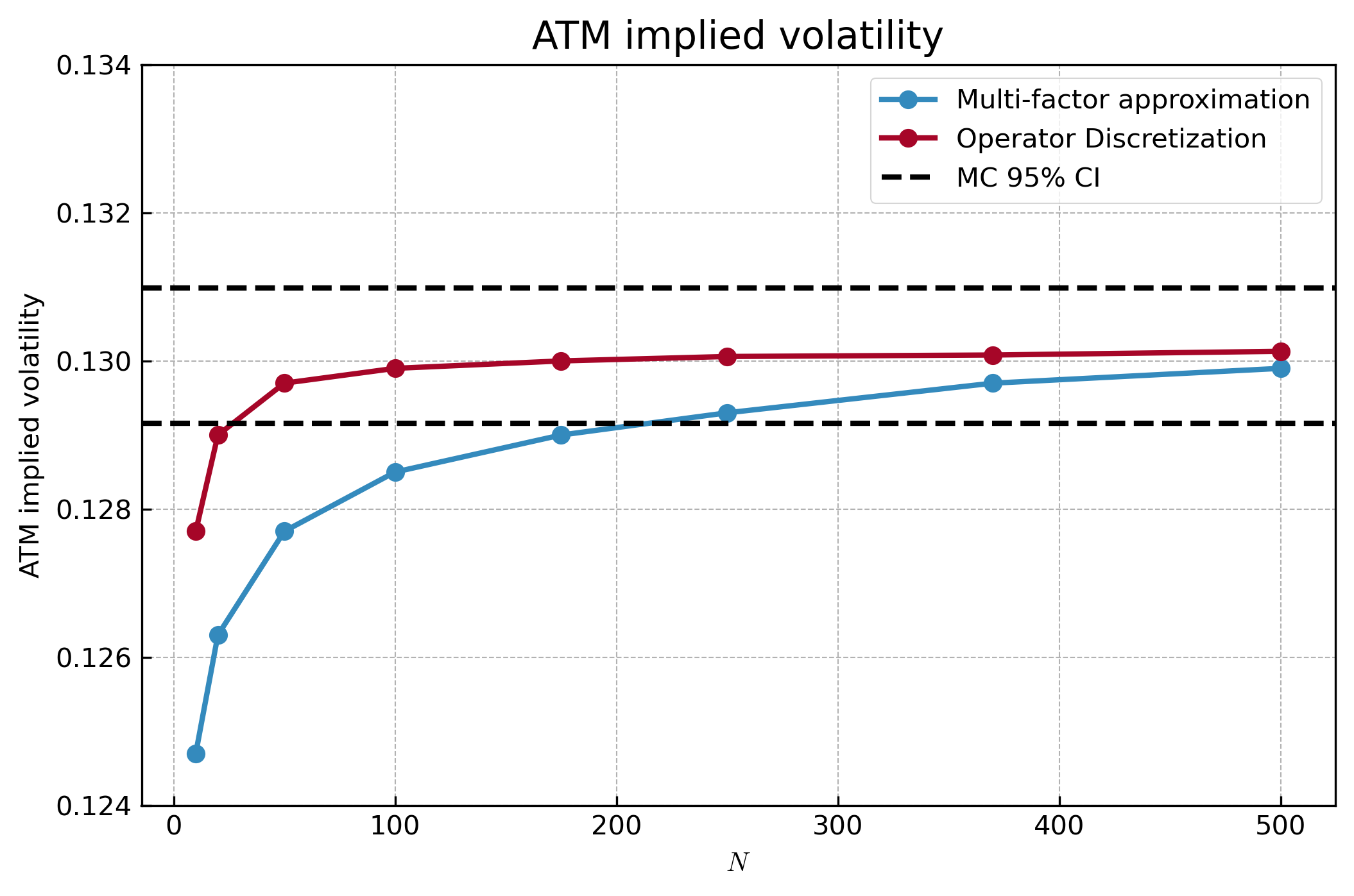
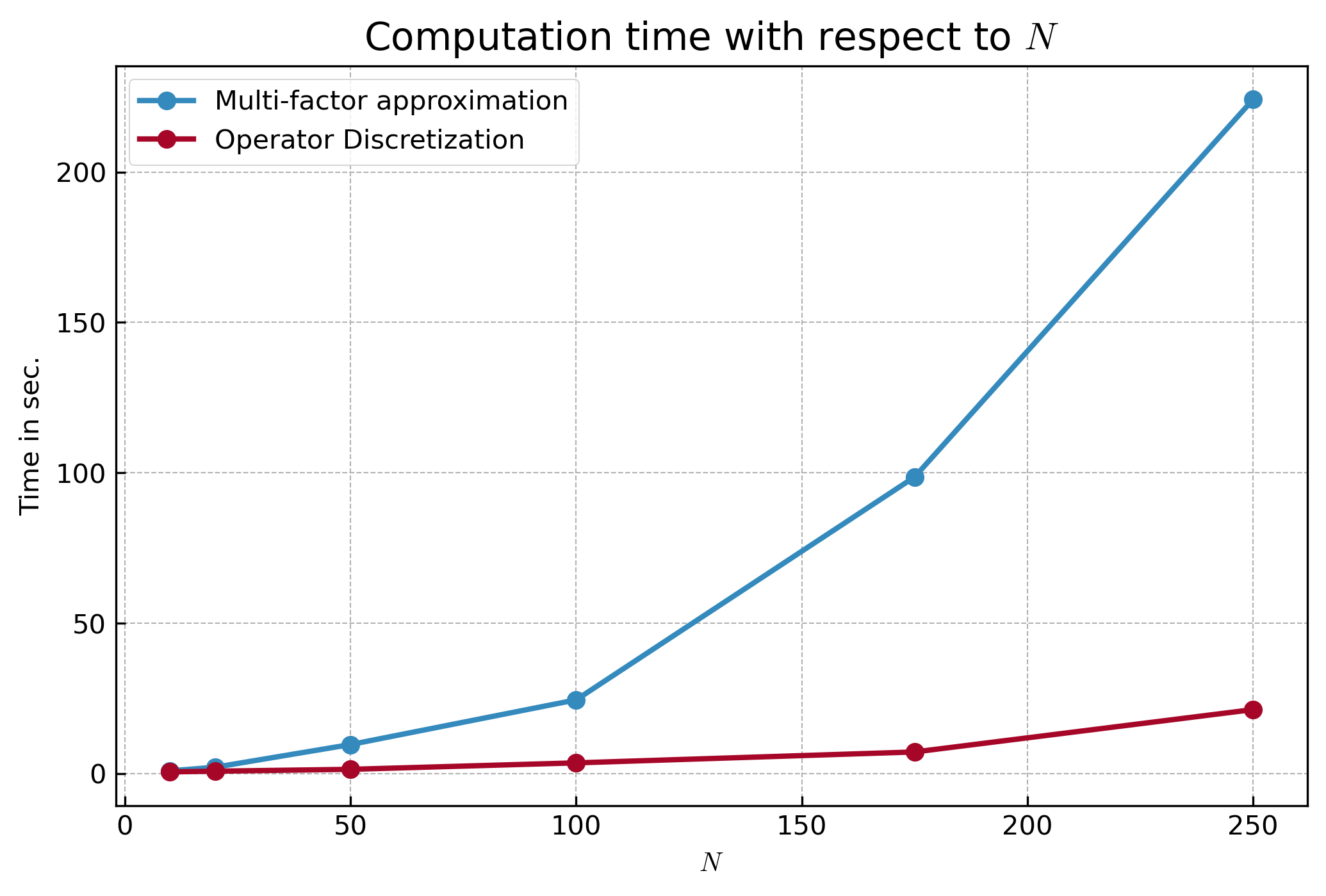
Figure 11: ATM forward implied volatility generated by the operator discretization and multi-factor approximation methods with $H_{\nu}=0.3$ (left) and the associated computation time (right).

6 Proofs

6.1 Proof of Theorem 3.1

We first consider two useful lemmas before proving Theorem 3.1.

Lemma 6.1.

For $u\in\mathbb{C}$ such that $0\leq\mathcal{\mathfrak{R}}(u)\leq 1,$ there exists an integral operator $\bar{\mathbf{\Psi}}_{t}^{u}$ induced by a symmetric kernel $\bar{\psi}_{t}^{u}(s,w)$ such that

$$\mathbf{\Psi}_{t}^{u}=a^{u}\text{id}+\bar{\mathbf{\Psi}}_{t}^{u},$$ (6.1)

and for any $f\in L^{2}([0,T],\mathbb{C}),$

$$(\mathbf{\Psi}_{t}^{u}f1_{t})(t)=(a^{u}\text{id}+b^{u}\mathbf{G}_{\nu}^{*}\mathbf{\Psi}_{t}^{u})(f1_{t})(t),$$ (6.2)

with $1_{t}:s\to 1_{t\leq s}.$ Moreover, the kernel $\bar{\psi}_{t}(s,w)$ satisfies

$$\bar{\psi}_{t}^{u}(t,s)=\bar{\psi}_{t}^{u}(s,t)=b^{u}\int_{t}^{T}G_{\nu}(w,t)(a\delta_{w=s}+\bar{\psi}_{t}^{u}(s,w))dw,\>t\leq s\leq T,\>a.e.$$ (6.3)

Proof.

From (Abi Jaber, 2022a, Lemma B.1.), we know that in our setting there exists an integral operator $\bar{\mathbf{\Psi}}_{t}^{u}$ induced by a symmetric kernel $\bar{\psi}_{t}(s,u)$ such that (6.1) and (6.2) are satisfied. Moreover, from (6.2), since $\mathbf{G}_{\nu}^{*}$ is an integral operator and $\bar{\psi}_{t}^{u}(s,w)$ is symmetric, we deduce that, for any $f\in L^{2}([0,T],\mathbb{C})$,

$$(\bar{\mathbf{\Psi}}_{t}^{u}f1_{t})(t) =(b^{u}\mathbf{G}_{\nu}^{*}\mathbf{\Psi}_{t}^{u})(f1_{t})(t)$$

$$=b^{u}\int_{t}^{T}G_{\nu}^{*}(t,s)\>(\mathbf{\Psi}_{t}^{u}f1_{t})(s)\>ds$$

$$=b^{u}\int_{t}^{T}G_{\nu}(s,t)\>\int_{t}^{T}(a^{u}\delta_{w=s}+\bar{\psi}_{t}^{u}(s,w))\>f(w)dw\>ds$$

$$=b^{u}\int_{t}^{T}f(s)\int_{t}^{T}G_{\nu}(w,t)(a^{u}\delta_{w=s}+\bar{\psi}_{t}^{u}(s,w))dw\>ds$$

Moreover, since $\bar{\mathbf{\Psi}}_{t}$ is a symmetric integral operator, we also have that

$$(\bar{\mathbf{\Psi}}_{t}^{u}f1_{t})(t) =\int_{t}^{T}\bar{\psi}_{t}^{u}(t,s)\>f(s)\>ds.$$

$$=\int_{t}^{T}\bar{\psi}_{t}^{u}(s,t)\>f(s)\>ds$$

We conclude that, for any $f\in L^{2}([0,T],\mathbb{C})$,

$$0 =\int_{t}^{T}f(s)\bigg{[}\bar{\psi}_{t}^{u}(s,t)-b^{u}\int_{t}^{T}G_{\nu}(w,t)(a^{u}\delta_{w=s}+\bar{\psi}_{t}^{u}(s,w))dw\bigg{]}\>ds$$

$$=\int_{t}^{T}f(s)\bigg{[}\bar{\psi}_{t}^{u}(t,s)-b^{u}\int_{t}^{T}G_{\nu}(w,t)(a^{u}\delta_{w=s}+\bar{\psi}_{t}^{u}(s,w))dw\bigg{]}\>ds,$$

and thus, for $t\leq s\leq T,$

$$\bar{\psi}_{t}^{u}(t,s)=\bar{\psi}_{t}^{u}(s,t)=b^{u}\int_{t}^{T}G_{\nu}(w,t)(a^{u}\delta_{w=s}+\bar{\psi}_{t}^{u}(s,w))dw,$$

almost everywhere. ∎

Lemma 6.2.

For $u\in\mathbb{C}$ such that $0\leq\mathcal{\mathfrak{R}}(u)\leq 1$ and $t\in[0,T],$ let us define $h_{t}^{u}(.)$ such that

$$h_{t}^{u}(s):=g_{t}(s)+1_{t\leq s}\bigg{(}\rho_{Ir}\eta_{r}B_{G_{r}}(s,T)-\int_{t}^{s}G_{\nu}(s,w)\>(b^{u}\rho_{Ir}-u\eta_{\nu}\rho_{\nu r})\eta_{r}B_{G_{r}}(w,T)\>dw\bigg{)},\;s,t\leq T.$$

Then the dynamics of $t\to\langle h_{t}^{u},\mathbf{\Psi}_{t}^{u}h_{t}^{u}\rangle_{L^{2}}$ is given by

$$d\langle h_{t}^{u},\mathbf{\Psi}_{t}^{u}h_{t}^{u}\rangle_{L^{2}}= \bigg{(}-a^{u}\bigg{(}\nu_{t}+\rho_{Ir}\eta_{r}B_{G_{r}}(t,T)\bigg{)}^{2}$$

$$-2u\eta_{\nu}(\rho_{I\nu}\nu_{t}+\rho_{\nu r}\eta_{r}B_{G_{r}}(t,T)(\mathbf{G}_{\nu}^{*}\mathbf{\Psi}_{t}^{u}h_{t})(t)$$

$$-Tr(\mathbf{\Psi}_{t}^{u}\dot{\mathbf{\Sigma}}_{t})+\langle h_{t}^{u},\dot{\mathbf{\Psi}}_{t}^{u}h_{t}^{u}\rangle_{L^{2}}\bigg{)}\>dt$$

$$+2\eta_{\nu}(\mathbf{G}_{\nu}^{*}\mathbf{\Psi}_{t}^{u}h_{t}^{u})(t)\>dW_{\nu}^{\mathbb{Q}^{T}}(t).$$ (6.4)

Proof.

First, we set

$$\bar{h}_{t}^{u}(s):= g_{0}^{T}(s)+\int_{0}^{t}G_{\nu}(s,w)\kappa_{\nu}\>\nu_{w}dw+\int_{0}^{t}G_{\nu}(s,w)\>\eta_{\nu}\>dW_{I}^{\mathbb{Q}^{T}}(w)$$

$$+ \bigg{(}\rho_{Ir}\eta_{r}B_{G_{r}}(s,T)-\int_{t}^{s}G_{\nu}(s,w)\>(b^{u}\rho_{Ir}-u\eta_{\nu}\rho_{\nu r})\eta_{r}B_{G_{r}}(w,T)\>dw\bigg{)}$$

and using Lemma 6.1, we have that

$$\langle h_{t}^{u},\mathbf{\Psi}_{t}^{u}h_{t}^{u}\rangle_{L^{2}}=\int_{t}^{T}(a^{u}\bar{h}_{t}^{u}(s)^{2}+\bar{h}_{t}^{u}(s)(\bar{\mathbf{\Psi}}_{t}^{u}h_{t}^{u})(s))\>ds.$$

Using the Leibniz rule, we deduce that

$$d\langle h_{t}^{u},\mathbf{\Psi}_{t}^{u}h_{t}^{u}\rangle_{L^{2}}= -(a^{u}\bar{h}_{t}^{u}(t)^{2}+\bar{h}_{t}^{u}(t)(\bar{\mathbf{\Psi}}_{t}^{u}h_{t}^{u})(t))dt$$

$$+\int_{t}^{T}d(a^{u}\bar{h}_{t}^{u}(s)^{2}+\bar{h}_{t}^{u}(s)(\bar{\mathbf{\Psi}}_{t}^{u}h_{t}^{u})(s))\>ds.$$

$$= -(a^{u}\bar{h}_{t}^{u}(t)^{2}+\bar{h}_{t}^{u}(t)(\bar{\mathbf{\Psi}}_{t}^{u}h_{t}^{u})(t))dt$$

$$+\int_{t}^{T}\bigg{(}a^{u}\,d(\bar{h}_{t}^{u}(s)^{2})+d\bar{h}_{t}^{u}(s)(\bar{\mathbf{\Psi}}_{t}^{u}h_{t}^{u})(s)+\bar{h}_{t}^{u}(s)d(\bar{\mathbf{\Psi}}_{t}^{u}h_{t}^{u})(s)$$

$$+d[\bar{h}_{t}^{u}(s),(\bar{\mathbf{\Psi}}_{t}^{u}h_{t}^{u})(s)]_{t}\bigg{)}\>ds.$$

For fixed $s\in[t,T],$ let us now deduce the dynamics of $t\to d\bar{h}_{t}^{u}(s),$ $t\to d(\bar{h}_{t}^{u}(s)^{2})$ and $t\to d(\bar{h}_{t}^{u}(s)(\bar{\mathbf{\Psi}}_{t}^{u}h_{t}^{u})(s)).$ Since we have that

$$d\bar{h}_{t}^{u}(s)=G_{\nu}(s,t)\bigg{(}\kappa_{\nu}\nu_{t}+(b^{u}\rho_{Ir}-u\eta_{\nu}\rho_{\nu r})\eta_{r}B_{G_{r}}(t,T)\bigg{)}dt+G_{\nu}(s,t)\eta_{\nu}\>dW_{\nu}^{\mathbb{Q}^{T}}(t),$$

an application of Ito’s lemma yields to

$$d(\bar{h}_{t}^{u}(s)^{2})= \bigg{(}\eta_{\nu}^{2}G_{\nu}(s,t)^{2}+2\bar{h}_{t}^{u}(s)G_{\nu}(s,t)\bigg{(}\kappa_{\nu}\nu_{t}+(b^{u}\rho_{Ir}-u\eta_{\nu}\rho_{\nu r})\eta_{r}B_{G_{r}}(t,T)\bigg{)}\bigg{)}dt$$

$$+2\bar{h}_{t}^{u}(s)G_{\nu}(s,t)\eta_{\nu}\>dW_{\nu}^{\mathbb{Q}^{T}}(t).$$

Moreover, an application of the Leibniz rule combined with the fact that $\bar{h}_{t}^{u}(t)=\nu_{t}+\rho_{Ir}\eta_{r}B_{G_{r}}(t,T)$ yields to

$$d(\bar{\mathbf{\Psi}}_{t}^{u}h_{t}^{u})(s)= \bigg{(}-\bar{\psi}_{t}^{u}(s,t)(\nu_{t}+\rho_{Ir}\eta_{r}B_{G_{r}}(t,T))+(\dot{\mathbf{\Psi}_{t}}^{u}h_{t}^{u})(s)$$

$$+\bigg{(}\kappa_{\nu}\nu_{t}+(b^{u}\rho_{Ir}-u\eta_{\nu}\rho_{\nu r})\eta_{r}B_{G_{r}}(t,T)\bigg{)}(\bar{\mathbf{\Psi}}_{t}^{u}G_{\nu}(.,t))(s)\bigg{)}\>\bigg{)}dt$$

$$+(\bar{\mathbf{\Psi}}_{t}^{u}G_{\nu}(.,t)\eta_{\nu})(s)\>dW_{\nu}^{\mathbb{Q}^{T}}(t),$$

The quadratic variation $t\to[\bar{h}_{t}^{u}(s),(\bar{\mathbf{\Psi}}_{t}^{u}h_{t})(s)]_{t}$ is given by

$$d[\bar{h}_{t}^{u}(s),(\bar{\mathbf{\Psi}}_{t}^{u}h_{t}^{u})(s)]_{t} =\eta_{\nu}^{2}\int_{0}^{T}\bar{\psi}_{t}^{u}(s,w)G_{\nu}(w,t)G_{\nu}(s,t)dwdt$$

$$=-\int_{0}^{T}\bar{\psi}_{t}^{u}(s,w)\dot{\Sigma}_{t}(w,s)dwdt$$

$$=-(\bar{\mathbf{\Psi}}_{t}^{u}\dot{\Sigma}_{t}(.,s))(s)dt.$$

Take it all together, we have that

$$a^{u}\,d(\bar{h}_{t}^{u}(s)^{2})+d\bar{h}_{t}^{u}(s)(\bar{\mathbf{\Psi}}_{t}^{u}h_{t}^{u})(s)+\bar{h}_{t}^{u}(s)d(\bar{\mathbf{\Psi}}_{t}^{u}h_{t}^{u})(s)+d[\bar{h}_{t}^{u}(s),(\bar{\mathbf{\Psi}}_{t}^{u}h_{t}^{u})(s)]_{t}$$

$$=\bigg{(} a^{u}\bigg{(}\eta_{\nu}^{2}G_{\nu}(s,t)^{2}+2\bar{h}_{t}^{u}(s)G_{\nu}(s,t)\bigg{(}\kappa_{\nu}\nu_{t}+(b^{u}\rho_{Ir}-u\eta_{\nu}\rho_{\nu r})\eta_{r}B_{G_{r}}(t,T)\bigg{)}\bigg{)}$$

$$+ G_{\nu}(s,t)\bigg{(}\kappa_{\nu}\nu_{t}+(b^{u}\rho_{Ir}-u\eta_{\nu}\rho_{\nu r})\eta_{r}B_{G_{r}}(t,T)\bigg{)}(\bar{\mathbf{\Psi}}_{t}^{u}h_{t}^{u})(s)$$

$$+ \bar{h}_{t}^{u}(s)\bigg{(}-\bar{\psi}_{t}^{u}(s,u)(\nu_{t}+\rho_{Ir}\eta_{r}B_{G_{r}}(t,T)+(\dot{\mathbf{\Psi}_{t}}^{u}h_{t}^{u})(s)$$

$$+ \bigg{(}\kappa_{\nu}\nu_{t}+(b^{u}\rho_{Ir}-u\eta_{\nu}\rho_{\nu r})\eta_{r}B_{G_{r}}(t,T)\bigg{)}(\bar{\mathbf{\Psi}}_{t}^{u}G_{\nu}(.,t))(s)\bigg{)}-(\bar{\mathbf{\Psi}}_{t}^{u}\dot{\Sigma}_{t}(.,s))(s)\bigg{)}\>dt$$

$$+ \bigg{(}2a^{u}\bar{h}_{t}^{u}(s)G_{\nu}(s,t)\eta_{\nu}+(\bar{\mathbf{\Psi}}_{t}^{u}h_{t}^{u})(s)G_{\nu}(s,t)\eta_{\nu}+\bar{h}_{t}^{u}(s)(\bar{\mathbf{\Psi}}_{t}^{u}G_{\nu}(.,t)\eta_{\nu})(s)\bigg{)}\>dW_{\nu}^{\mathbb{Q}^{T}}(t).$$

Therefore, we obtain that

$$d\langle h_{t}^{u},\mathbf{\Psi}_{t}^{u}h_{t}^{u}\rangle_{L^{2}}= \bigg{(}-(a^{u}(\nu_{t}+\rho_{Ir}\eta_{r}B_{G_{r}}(t,T))^{2}$$

$$-2(\nu_{t}+\rho_{Ir}\eta_{r}B_{G_{r}}(t,T))(\bar{\mathbf{\Psi}}_{t}^{u}h_{t}^{u})(t)$$

$$+2(\kappa_{\nu}\nu_{t}+(b^{u}\rho_{Ir}-u\eta_{\nu}\rho_{\nu r})\eta_{r}B_{G_{r}}(t,T))(\mathbf{G}_{\nu}^{*}\mathbf{\Psi}_{t}^{u}h_{t})(t)$$

$$+\langle h_{t}^{u},\dot{\mathbf{\Psi}}_{t}^{u}h_{t}^{u}\rangle_{L^{2}}-\text{Tr}(\mathbf{\Psi}_{t}^{u}\dot{\mathbf{\Sigma}}_{t})\bigg{)}\>dt$$

$$+2\eta_{\nu}(\mathbf{G}_{\nu}^{*}\mathbf{\Psi}_{t}^{u}h_{t}^{u})(t)\>dW_{\nu}^{\mathbb{Q}^{T}}(t).$$

Finally, using the fact that $b^{u}=\kappa_{\nu}+u\eta_{\nu}\rho_{I\nu}$ and $(\bar{\mathbf{\Psi}}_{t}^{u}h_{t}^{u})(t)=b^{u}(\mathbf{G}_{\nu}^{*}\mathbf{\Psi}_{t}^{u}h_{t}^{u})(t)$ (see Lemma 6.1), we obtain that

$$d\langle h_{t}^{u},\mathbf{\Psi}_{t}^{u}h_{t}^{u}\rangle_{L^{2}}= \bigg{(}-a^{u}(\nu_{t}+\rho_{Ir}\eta_{r}B_{G_{r}}(t,T))^{2}$$

$$-2u\eta_{\nu}(\rho_{I\nu}\nu_{t}+\rho_{\nu r}\eta_{r}B_{G_{r}}(t,T))(\mathbf{G}_{\nu}^{*}\mathbf{\Psi}_{t}^{u}h_{t})(t)$$

$$-\text{Tr}(\mathbf{\Psi}_{t}^{u}\dot{\mathbf{\Sigma}}_{t})+\langle h_{t}^{u},\dot{\mathbf{\Psi}}_{t}^{u}h_{t}^{u}\rangle_{L^{2}}\bigg{)}\>dt$$

$$+2\eta_{\nu}(\mathbf{G}_{\nu}^{*}\mathbf{\Psi}_{t}^{u}h_{t}^{u})(t)\>dW_{\nu}^{\mathbb{Q}^{T}}(t).$$

∎

Based now of Lemma 6.1 and 6.2, we are now ready to prove Theorem 3.1.

Proof.

As explained in Abi Jaber (2022a), it is sufficient to make the proof for $u\in\mathbb{R}$ such $0\leq u\leq 1.$ Fix $u\in[0,1]$ and consider the processes $(U_{t})_{0\leq t\leq T}$ and $(M_{t})_{0\leq t\leq T}$ defined, for $t\in[0,T],$ by

$$U_{t}=u\log I_{t}^{T}+\phi_{t}^{u}+\chi_{t}^{u}+\langle h_{t}^{u},\mathbf{\Psi}_{t}^{u}h_{t}^{u}\rangle_{L^{2}},$$ (6.5)

and

$$M_{t}=\exp(U_{t}).$$

If we prove that $(M_{t})_{0\leq t\leq T}$ is a martingale under $\mathbb{Q}^{T}$, then the proof is complete since, in this case, we have that

$$E^{\mathbb{Q}^{T}}(M_{T}|\mathcal{F}_{t})=M_{t},$$

and thus

$$E^{\mathbb{Q}^{T}}\bigg{[}\exp\bigg{(}u\log\frac{I_{T}^{T}}{I_{t}^{T}}\bigg{)}\bigg{|}\mathcal{F}_{t}\bigg{]}=\exp(\phi_{t}^{u}+\chi_{t}^{u}+\langle h_{t}^{u},\mathbf{\Psi}_{t}^{u}h_{t}^{u}\rangle_{L^{2}}).$$

Let us prove that $(M_{t})_{0\leq t\leq T}$ is a (true) martingale under $\mathbb{Q}^{T}$. First, we can prove that $(M_{t})_{0\leq t\leq T}$ is a local martingale by showing that the drift of the dynamic of $(M_{t})_{0\leq t\leq T}$ is null. Using the dynamic of $(I_{t}^{T})_{0\leq t\leq T}$ given by (2.12), the dynamic of $(\langle h_{t}^{u},\mathbf{\Psi}_{t}^{u}h_{t}^{u}\rangle_{L^{2}})_{0\leq t\leq T}$ given by (6.4) and the fact that $a^{u}=\frac{1}{2}(u^{2}-u)$, we observe that

$$dU_{t}= u\>d(\log I_{t}^{T})+(\dot{\phi}_{t}^{u}+\dot{\chi}_{t}^{u})dt+d\langle h_{t}^{u},\mathbf{\Psi}_{t}^{u}h_{t}^{u}\rangle_{L^{2}}$$

$$= \bigg{(}-\frac{u^{2}}{2}\bigg{(}\nu_{t}^{2}+\eta_{r}^{2}B_{G_{r}}(t,T)^{2}+2\nu_{t}\eta_{r}B_{G_{r}}(t,T)\rho_{Ir}\bigg{)}$$

$$+\langle h_{t}^{u},\dot{\mathbf{\Psi}}_{t}^{u}h_{t}^{u}\rangle_{L^{2}}-2u\eta_{\nu}(\rho_{I\nu}\nu_{t}+\rho_{\nu r}\eta_{r}B_{G_{r}}(t,T))(\mathbf{G}_{\nu}^{*}\mathbf{\Psi}_{t}^{u}h_{t}^{u})(t)\>\bigg{)}\>dt$$

$$+u\nu_{t}\>dW_{I}^{\mathbb{Q}^{T}}(t)+u\eta_{r}B_{G_{r}}(t,T)dW_{r}^{\mathbb{Q}^{T}}(t)+2\eta_{\nu}(\mathbf{G}_{\nu}^{*}\mathbf{\Psi}_{t}^{u}h_{t}^{u})(t))\>dW_{\nu}^{\mathbb{Q}^{T}}(t).$$

Moreover, the quadratic variation of $(U_{t})_{0\leq t\leq T}$ satisfies

$$d\langle U\rangle_{t}= \bigg{(}(u^{2}\nu_{t}^{2}+4\eta_{\nu}^{2}(\mathbf{G}_{\nu}^{*}\mathbf{\Psi}_{t}^{u}h_{t}^{u})(t))^{2}+u^{2}\eta_{r}^{2}B_{G_{r}}(t,T)^{2}$$

$$+2u^{2}\nu_{t}\rho_{Ir}\eta_{r}B_{G_{r}}(t,T)$$

$$+4u\eta_{\nu}(\mathbf{G}_{\nu}^{*}\mathbf{\Psi}_{t}^{u}h_{t}^{u})(t))\bigg{(}\rho_{I\nu}\nu_{t}+\rho_{r\nu}\eta_{r}B_{G_{r}}(t,T)\bigg{)}\>\bigg{)}dt.$$

As the dynamic of $(M_{t})_{0\leq t\leq T}$ can be written such that

$$dM_{t}=M_{t}\,\bigg{(}\frac{1}{2}d\langle U\rangle_{t}+dU_{t}\bigg{)},$$

we easily obtain that

$$dM_{t}= M_{t}\,\bigg{(}2\eta_{\nu}^{2}((\mathbf{G}_{\nu}^{*}\mathbf{\Psi}_{t}^{u}h_{t}^{u})(t))^{2}+\langle h_{t}^{u},\dot{\mathbf{\Psi}}_{t}^{u}h_{t}^{u}\rangle_{L^{2}}\bigg{)}\>dt$$

$$+M_{t}\,\bigg{(}u\nu_{t}\>dW_{I}^{\mathbb{Q}^{T}}(t)+u\eta_{r}B_{G_{r}}(t,T)dW_{r}^{\mathbb{Q}^{T}}(t)+2\eta_{\nu}(\mathbf{G}_{\nu}^{*}\mathbf{\Psi}_{t}^{u}h_{t}^{u})(t))\>dW_{\nu}^{\mathbb{Q}^{T}}(t)\bigg{)},$$

but as

$$2\eta_{\nu}^{2}((\mathbf{G}_{\nu}^{*}\mathbf{\Psi}_{t}^{u}h_{t}^{u})(t))^{2}=-2\langle h_{t}^{u},\mathbf{\Psi}_{t}^{u}\dot{\mathbf{\Sigma}}_{t}\mathbf{\Psi}_{t}^{u}h_{t}^{u}\rangle_{L^{2}},$$

we have that

$$dM_{t}= M_{t}\,\bigg{(}\langle h_{t}^{u},(\dot{\mathbf{\Psi}}_{t}^{u}-2\mathbf{\Psi}_{t}^{u}\dot{\mathbf{\Sigma}}_{t}\mathbf{\Psi}_{t}^{u})h_{t}^{u}\rangle_{L^{2}}\bigg{)}\>dt$$

$$+M_{t}\,\bigg{(}u\nu_{t}\>dW_{I}^{\mathbb{Q}^{T}}(t)+u\eta_{r}B_{G_{r}}(t,T)dW_{r}^{\mathbb{Q}^{T}}(t)+2\eta_{\nu}(\mathbf{G}_{\nu}^{*}\mathbf{\Psi}_{t}^{u}h_{t}^{u})(t))\>dW_{I}^{\mathbb{Q}^{T}}(t)\bigg{)}$$

$$= M_{t}\,\bigg{(}u\nu_{t}\>dW_{I}^{\mathbb{Q}^{T}}(t)+u\eta_{r}B_{G_{r}}(t,T)dW_{r}^{\mathbb{Q}^{T}}(t)+2\eta_{\nu}(\mathbf{G}_{\nu}^{*}\mathbf{\Psi}_{t}^{u}h_{t}^{u})(t))\>dW_{I}^{\mathbb{Q}^{T}}(t)\bigg{)},$$

and since, from (Abi Jaber, 2022a, Lemma B.1.),

$$\dot{\mathbf{\Psi}}_{t}^{u}-2\mathbf{\Psi}_{t}^{u}\dot{\mathbf{\Sigma}}_{t}\mathbf{\Psi}_{t}^{u}=0,$$

we have that $(M_{t})_{0\leq t\leq T}$ is a local martingale. It remains to show that this is a true martingale. Since $\langle h_{t}^{u},\dot{\mathbf{\Psi}}_{t}^{u}h_{t}^{u}\rangle_{L^{2}}\leq 0$ and $\phi_{t}^{u}=-\int_{t}^{T}Tr(\mathbf{\Psi}_{s}^{u}\dot{\mathbf{\Sigma}}_{s})\>ds\leq 0$, from (6.5), it follows that

$$U_{t}\leq u\log I_{t}^{T}+\chi_{t}^{u}.$$

Furthermore, we observe that

$$U_{t}\leq u\log I_{0}^{T}-\frac{u}{2}^{2}\int_{0}^{t}\bigg{(}\,\bigg{(}\nu_{s}+\rho_{Ir}\eta_{r}B_{G_{r}}(s,T)\bigg{)}^{2}+(1-\rho_{Ir}^{2})\eta_{r}^{2}B_{G_{r}}(s,T)^{2}\bigg{)}\>ds$$

$$+\frac{1}{2}(u^{2}-u)\bigg{(}\int_{0}^{T}(1-\rho_{Ir}^{2})\eta_{r}^{2}B_{G_{r}}(s,T)^{2}\>ds\bigg{)}$$

$$+\int_{0}^{t}u\nu_{s}\>dW_{I}^{\mathbb{Q}^{T}}(s)+\int_{0}^{t}u\eta_{r}B_{G_{r}}(s,T)dW_{r}^{\mathbb{Q}^{T}}(s),$$

and, as $u\in[0,1],$ we deduce that

$$U_{t}\leq u\log I_{0}^{T}-\frac{u}{2}^{2}\int_{0}^{t}\bigg{(}\,\bigg{(}\nu_{s}+\rho_{Ir}\eta_{r}B_{G_{r}}(s,T)\bigg{)}^{2}+(1-\rho_{Ir}^{2})\eta_{r}^{2}B_{G_{r}}(s,T)^{2}\bigg{)}\>ds$$

$$+\int_{0}^{t}u\nu_{s}\>dW_{I}^{\mathbb{Q}^{T}}(s)+\int_{0}^{t}u\eta_{r}B_{r}(s,T)dW_{r}^{\mathbb{Q}^{T}}(s).$$

Then, we define the process $(N_{t})_{0\leq t\leq T}$ such that

$$N_{t}:= \bigg{(}I_{0}^{T}\bigg{)}^{u}\exp\bigg{(}-\frac{u}{2}^{2}\int_{0}^{t}\bigg{(}\,\bigg{(}\nu_{s}+\rho_{Ir}\eta_{r}B_{G_{r}}(s,T)\bigg{)}^{2}+(1-\rho_{Ir}^{2})\eta_{r}^{2}B_{G_{r}}(s,T)^{2}\bigg{)}\>ds$$

$$+\int_{0}^{t}u\nu_{s}\>dW_{I}^{\mathbb{Q}^{T}}(s)+\int_{0}^{t}u\eta_{r}B_{G_{r}}(s,T)dW_{r}^{\mathbb{Q}^{T}}(s)\bigg{)},$$

This process $(N_{t})_{0\leq t\leq T}$ is a true martingale (see arguments in (Abi Jaber et al., 2021b, in Lemma 7.3)). Therefore, we finally have that

$$|M_{t}|\leq\exp(U_{t})\leq N_{t}$$

and as $(M_{t})_{0\leq t\leq T}$ is a local martingale upper bounded by a true martingale, this a true martingale and it completes the proof. ∎

6.2 Proof of Proposition 5.2

We first consider a lemma before proving Proposition 5.2.

Lemma 6.3.

Assume that the kernel function $G_{\nu}(t,s)$ is completely monotone and can be represented as (5.3). Then,

$$\nu_{t}=g_{0}^{T}(t)+\int_{\mathbb{R}_{+}}Y_{t}(x)\>\lambda(dx),\>t\leq T,$$

$$g_{t}(s)=1_{t\leq s}\bigg{(}g_{0}^{T}(s)+\int_{\mathbb{R}_{+}}e^{-x(s-t)}Y_{t}(x)\>\lambda(dx)\bigg{)},$$

with

$$Y_{t}(x)=\int_{0}^{t}e^{-(t-w)x}\kappa_{\nu}\>\nu_{w}\>dw+\int_{0}^{t}e^{-(t-w)x}\eta_{\nu}\>dW_{\nu}^{\mathbb{Q}^{T}}(w),\>t\leq T,\>x\in\mathbb{R}_{+}.$$ (6.6)

Moreover, for $u\in\mathbb{C}$ such that $0\leq\mathcal{\mathfrak{R}}(u)\leq 1,$

$$h_{t}^{u}(s)=g_{t}(s)+1_{t\leq s}\bigg{(}\rho_{Ir}\eta_{r}B_{G_{t}}(s,T)-\int_{\mathbb{R}_{+}}b_{t}^{u}(s,x)\>\lambda(dx)\bigg{)},$$

with

$$b_{t}^{u}(s,x)=\int_{t}^{s}e^{-(s-w)x}\bigg{(}(b^{u}\rho_{Ir}-u\eta_{\nu}\rho_{\nu r})\eta_{r}B_{G_{r}}(w,T)\bigg{)}\>dw,\>t\leq s\leq T,\>x\in\mathbb{R}_{+}.$$ (6.7)

Proof.

For $t\leq T$, applying Fubini’s theorem, we can rewrite $\nu_{t}$ such that

$$\nu_{t} =g_{0}^{T}(s)+\int_{0}^{t}G_{\nu}(t,w)\kappa_{\nu}\>\nu_{u}dw+\int_{0}^{t}G_{\nu}(t,w)\eta_{\nu}\>dW_{\nu}^{\mathbb{Q}^{T}}(w)$$

$$=g_{0}^{T}(s)+\int_{0}^{t}\int_{\mathbb{R}_{+}}e^{-(t-w)x}\lambda(dx)\kappa_{\nu}\>\nu_{w}dw+\int_{0}^{t}\int_{\mathbb{R}_{+}}e^{-(t-w)x}\lambda(dx)\eta_{\nu}\>dW_{\nu}^{\mathbb{Q}^{T}}(w)$$

$$=g_{0}^{T}(s)+\int_{\mathbb{R}_{+}}\bigg{(}\int_{0}^{t}e^{-(t-w)x}\kappa_{\nu}\>\nu_{w}dw+\int_{0}^{t}e^{-(t-w)x}\eta_{\nu}\>dW_{\nu}^{\mathbb{Q}^{T}}(w)\bigg{)}\>\lambda(dx)$$

$$=g_{0}^{T}(s)+\int_{\mathbb{R}_{+}}Y_{t}(x)\>\lambda(dx),$$

with $Y_{t}(x)$ given by (6.6). Using the same arguments, we obtain that,

$$g_{t}(s)=1_{t\leq s}\bigg{(}g_{0}^{T}(s)+\int_{\mathbb{R}_{+}}e^{-x(s-t)}Y_{t}(x)\>\lambda(dx)\bigg{)}.$$

Finally, we have that,

$$h_{t}^{u}(s)= g_{t}(s)+1_{t\leq s}\bigg{(}\rho_{Ir}\eta_{r}B_{G_{r}}(s,T)-\int_{t}^{s}G_{\nu}(s,w)\bigg{(}(b^{u}\rho_{Ir}-u\eta_{\nu}\rho_{\nu r})\eta_{r}B_{G_{r}}(w,T)\bigg{)}dw\bigg{)}$$

$$= g_{t}(s)+1_{t\leq s}\bigg{(}\rho_{Ir}\eta_{r}B_{G_{r}}(s,T)-\int_{\mathbb{R}_{+}}\bigg{(}\int_{t}^{s}e^{-(s-w)x}\bigg{(}(b^{u}\rho_{Ir}-u\eta_{\nu}\rho_{\nu r})\eta_{r}B_{G_{r}}(w,T)\bigg{)}\>dw\bigg{)}\>\lambda(dx)\bigg{)}$$

$$= g_{t}(s)+1_{t\leq s}\bigg{(}\rho_{Ir}\eta_{r}B_{G_{r}}(s,T)-\int_{\mathbb{R}_{+}}b_{t}^{u}(s,x)\>\lambda(dx)\bigg{)},$$

with $b_{t}^{u}(s,x)$ given by (6.7). ∎

Proof.

We divide the proof into two steps. The first step is to show that

$$E^{\mathbb{Q}^{T}}\bigg{[}\exp\bigg{(}u\log\frac{I_{T}^{T}}{I_{t}^{T}}\bigg{)}\bigg{|}\mathcal{F}_{t}\bigg{]}=\exp\bigg{(}\Theta_{t}^{u}+2\int_{\mathbb{R}_{+}}\Lambda_{t}^{u}(x)Y_{t}(x)\>\lambda(dx)+\int_{\mathbb{R}_{+}^{2}}\Gamma_{t}^{u}(x,y)Y_{t}(x)Y_{t}(y)\>\lambda(dx)\>\lambda(dy)\bigg{)},$$

with $t\to(\Theta_{t}^{u},\Lambda_{t}^{u},\Gamma_{t}^{u})$ such that

$$\Theta_{t}^{u}:=\phi_{t}^{u}+\chi_{t}^{u}+\int_{t}^{T}a^{u}\bar{h}_{t}^{u}(s)^{2}ds+\int_{t}^{T}\int_{t}^{T}\bar{h}_{t}^{u}(s)\bar{h}_{t}(w)\bar{\psi}_{t}^{u}(s,w)dsdw,$$ (6.8)

$$\Lambda_{t}(x):=\int_{t}^{T}a^{u}\bar{h}_{t}^{u}(s)e^{-x(s-t)}\,ds+\int_{t}^{T}\int_{t}^{T}\bar{h}_{t}^{u}(w)e^{-x(s-t)}\bar{\psi}_{t}^{u}(s,w)\,dsdw,\>x\in\mathbb{R}_{+},$$ (6.9)

and

$$\Gamma_{t}(x,y):=\int_{t}^{T}\int_{t}^{T}e^{-x(s-t)}e^{-y(w-t)}\>(a^{u}\delta_{s=w}+\bar{\psi}_{t}^{u}(s,w))\>ds\,dw,\>(x,y)\in\mathbb{R}_{+}^{2},$$ (6.10)

with $\bar{h}_{t}^{u}(s)$ a time-dependent function given by

$$\bar{h}_{t}^{u}(s):=1_{t\leq s}\bigg{(}g_{0}^{T}(s)+\rho_{Ir}\eta_{r}B_{G_{r}}(s,T)-\int_{\mathbb{R}_{+}}b_{t}^{u}(s,x)\>\lambda(dx)\bigg{)}.$$ (6.11)

Then, the second step is to deduce the equations satisfied by $(\Theta_{t}^{u},\Lambda_{t}^{u},\Gamma_{t}^{u})$.

Step 1

Using Proposition 5.1, we have that

$$E^{\mathbb{Q}^{T}}\bigg{[}\exp\bigg{(}u\log\frac{I_{T}^{T}}{I_{t}^{T}}\bigg{)}\bigg{|}\mathcal{F}_{t}\bigg{]}=\exp(\phi_{t}^{u}+\chi_{t}^{u}+a^{u}\int_{t}^{T}h_{t}^{u}(s)^{2}ds+\int_{t}^{T}\int_{t}^{T}h_{t}^{u}(s)h_{t}^{u}(w)\>\bar{\psi}_{t}^{u}(s,w)dsdw).$$

Moreover, from Lemma 6.3, we have that

$$h_{t}^{u}(s)=\bar{h}_{t}^{u}(s)+1_{t\leq s}\int_{\mathbb{R}_{+}}e^{-x(s-t)}Y_{t}(x)\>\lambda(dx),$$

with $\bar{h}_{t}^{u}(s)$ given by (6.11).
Therefore, using once again Fubini’s theorem, we have that

$$\int_{t}^{T}h_{t}^{u}(s)^{2}ds= \int_{t}^{T}\bigg{(}\bar{h}_{t}^{u}(s)+\int_{\mathbb{R}_{+}}e^{-x(s-t)}Y_{t}(x)\>\lambda(dx)\bigg{)}\>\bigg{(}\bar{h}_{t}^{u}(s)+\int_{\mathbb{R}_{+}}e^{-y(s-t)}Y_{t}(y)\>\lambda(dy)\bigg{)}ds$$

$$= \int_{t}^{T}\bigg{(}\bar{h}_{t}^{u}(s)^{2}+2\bar{h}_{t}^{u}(s)\int_{\mathbb{R}_{+}}e^{-x(s-t)}Y_{t}(x)\>\lambda(dx)+\int_{\mathbb{R}_{+}^{2}}e^{-x(s-t)}e^{-y(s-t)}Y_{t}(x)\>Y_{t}(y)\>\lambda(dx)\>\lambda(dy)\bigg{)}ds$$

$$= \int_{t}^{T}\bar{h}_{t}^{u}(s)^{2}ds+\int_{\mathbb{R}_{+}}\bigg{(}\int_{t}^{T}2\bar{h}_{t}^{u}(s)e^{-x(s-t)}\,ds\bigg{)}\>Y_{t}(x)\>\lambda(dx)$$

$$+\int_{\mathbb{R}_{+}^{2}}\bigg{(}\int_{t}^{T}e^{-x(s-t)}e^{-y(s-t)}ds\bigg{)}Y_{t}(x)\>Y_{t}(y)\>\lambda(dx)\>\lambda(dy),$$

and

$$\int_{t}^{T}\int_{t}^{T}h_{t}^{u}(s)h_{t}^{u}(w)\>\bar{\psi}_{t}^{u}(s,w)dsdw= \int_{t}^{T}\int_{t}^{T}\bar{h}_{t}^{u}(s)\bar{h}_{t}^{u}(w)\bar{\psi}_{t}^{u}(s,w)dsdw$$

$$+\int_{\mathbb{R}_{+}}\bigg{(}\int_{t}^{T}\int_{t}^{T}2\bar{h}_{t}^{u}(w)e^{-x(s-t)}\bar{\psi}_{t}^{u}(s,w)\,dsdw\bigg{)}\>Y_{t}(x)\>\lambda(dx)$$

$$+\int_{\mathbb{R}_{+}^{2}}\bigg{(}\int_{t}^{T}\int_{t}^{T}e^{-x(s-t)}e^{-y(u-t)}\bar{\psi}_{t}^{u}(s,w)ds\,dw\bigg{)}Y_{t}(x)\>Y_{t}(y)\>\lambda(dx)\>\lambda(dy).$$

Thus, we have that

$$a^{u}\int_{t}^{T}h_{t}^{u}(s)^{2}ds+\int_{t}^{T}\int_{t}^{T}h_{t}^{u}(s)h_{t}^{u}(w)\>\bar{\psi}_{t}^{u}(s,w)dsdw= \int_{t}^{T}a^{u}\bar{h}_{t}^{u}(s)^{2}ds+\int_{t}^{T}\int_{t}^{T}\bar{h}_{t}^{u}(s)\bar{h}_{t}^{u}(w)\bar{\psi}_{t}^{u}(s,w)dsdw$$

$$+2\int_{\mathbb{R}_{+}}\bigg{(}\int_{t}^{T}a^{u}\bar{h}_{t}^{u}(s)e^{-x(s-t)}\,ds$$

$$\;\;\;\;\;\;\;+\int_{t}^{T}\int_{t}^{T}\bar{h}_{t}^{u}(w)e^{-x(s-t)}\bar{\psi}_{t}^{u}(s,w)\,dsdw\bigg{)}\>Y_{t}(x)\>\lambda(dx)$$

$$+\int_{\mathbb{R}_{+}^{2}}\bigg{(}\int_{t}^{T}\int_{t}^{T}e^{-x(s-t)}e^{-y(w-t)}\>(a^{u}\delta_{s=w}$$

$$\;\;\;\;\;\;\;\;\;\;\;\;\;\;+\bar{\psi}_{t}^{u}(s,w))\>ds\,dw\bigg{)}Y_{t}(x)\>Y_{t}(y)\>\lambda(dx)\>\lambda(dy).$$

By defining $t\to(\Theta_{t}^{u},\Lambda_{t}^{u},\Gamma_{t}^{u})$ by (6.8)-(6.9)-(6.10), we obtain that

$$E^{\mathbb{Q}^{T}}\bigg{[}\exp\bigg{(}u\log\frac{I_{T}^{T}}{I_{t}^{T}}\bigg{)}\bigg{|}\mathcal{F}_{t}\bigg{]}=\exp\bigg{(}\Theta_{t}^{u}+2\int_{\mathbb{R}_{+}}\Lambda_{t}^{u}(x)Y_{t}(x)\>\lambda(dx)+\int_{\mathbb{R}_{+}^{2}}\Gamma_{t}^{u}(x,y)Y_{t}(x)Y_{t}(y)\>\lambda(dx)\>\lambda(dy)\bigg{)}.$$

Step 2

Let us now deduce the equations satisfied by $(\Theta_{t}^{u},\Lambda_{t}^{u},\Gamma_{t}^{u})$. First, we have that

$$\Gamma_{t}^{u}(x,y)=\int_{t}^{T}\int_{t}^{T}e^{-x(s-t)}e^{-y(w-t)}\bigg{(}a^{u}\delta_{s=w}+\bar{\psi}_{t}^{u}(s,w)\bigg{)}ds\,dw.$$

A direct differentiation of $t\to\Gamma_{t}^{u}$ with respect to $t$ leads to

$$\dot{\Gamma}_{t}^{u}(x,y)= (x+y)\Gamma_{t}^{u}(x,y)-a^{u}-\int_{t}^{T}\bigg{(}e^{-x(s-t)}+e^{-y(s-t)}\bigg{)}\>\bar{\psi}_{t}^{u}(s,t)ds$$

$$+\int_{t}^{T}\int_{t}^{T}e^{-x(s-t)}e^{-y(w-t)}\dot{\bar{\psi}}_{t}^{u}(s,w)ds\,dw.$$

Using the form of $\dot{\bar{\psi}}_{t}^{u}(s,w),$ we obtain that

$$\int_{t}^{T}\int_{t}^{T}e^{-x(s-t)}e^{-y(w-t)}\dot{\bar{\psi}}_{t}^{u}(s,w)ds\,dw=-2\,\eta_{\nu}^{2}\bigg{(}\int_{\mathbb{R}_{+}}\Gamma_{t}^{u}(x,x^{\prime})\>\lambda(dx^{\prime})\bigg{)}\bigg{(}\int_{\mathbb{R}_{+}}\Gamma_{t}^{u}(y,y^{\prime})\>\lambda(dy^{\prime})\bigg{)}.$$

Moreover, using (6.3) in Lemma 6.1 and once again the Fubini’s theorem, we have that

$$\int_{t}^{T}e^{-x(s-t)}\>(\bar{\psi}_{t}^{u}(s,t))ds =b^{u}\int_{t}^{T}e^{-x(s-t)}\int_{t}^{T}G_{\nu}(w,t)(a^{u}\delta_{w=s}+\bar{\psi}_{t}^{u}(s,w))dwds$$

$$=b^{u}\bigg{(}\int_{t}^{T}e^{-x(s-t)}\int_{t}^{T}\bigg{(}\int_{\mathbb{R}_{+}}e^{-x^{{}^{\prime}}(w-t)}\>\lambda(dx^{\prime})\bigg{)}\>(a^{u}\delta_{w=s}+\bar{\psi}_{t}^{u}(s,w)\>dwds$$

$$=b^{u}\int_{\mathbb{R}_{+}}\bigg{(}\int_{t}^{T}\int_{t}^{T}e^{-x^{{}^{\prime}}(w-t)}e^{-x(s-t)}\bigg{(}a^{u}\delta_{w=s}+\bar{\psi}_{t}^{u}(s,w)\bigg{)}\>dwds\bigg{)}\>\lambda(dx^{\prime})$$

$$=b^{u}\int_{\mathbb{R}_{+}}\Gamma_{t}(x,x^{{}^{\prime}})\>\lambda(dx^{\prime}).$$

Using the same arguments, we also obtain that

$$\int_{t}^{T}e^{-y(s-t)}\>(a^{u}\delta_{s=w}+\bar{\psi}_{t}^{u}(s,t))ds=b^{u}\int_{\mathbb{R}_{+}}\Gamma_{t}^{u}(y^{{}^{\prime}},y)\>\lambda(dy^{\prime}).$$

Thus, we deduce that

$$\dot{\Gamma}_{t}^{u}(x,y)= (x+y)\Gamma_{t}^{u}(x,y)-a^{u}-2\,\eta_{\nu}^{2}\bigg{(}\int_{\mathbb{R}_{+}}\Gamma_{t}^{u}(x,x^{\prime})\>\lambda(dx^{\prime})\bigg{)}\bigg{(}\int_{\mathbb{R}_{+}}\Gamma_{t}^{u}(y,y^{\prime})\>\lambda(dy^{\prime})\bigg{)}$$

$$-b^{u}\bigg{(}\int_{\mathbb{R}_{+}}\Gamma_{t}^{u}(x,x^{{}^{\prime}})\>\lambda(dx^{\prime})+\int_{\mathbb{R}_{+}}\Gamma_{t}^{u}(y^{{}^{\prime}},y)\>\lambda(dy^{\prime})\bigg{)}.$$

Let us consider now the ODE satisfied by $t\to\Lambda_{t}^{u}$. We have that

$$\Lambda_{t}^{u}(x) =\int_{t}^{T}a^{u}\bar{h}_{t}^{u}(s)e^{-x(s-t)}\,ds+\int_{t}^{T}\int_{t}^{T}\bar{h}_{t}^{u}(w)e^{-x(s-t)}\bar{\psi}_{t}^{u}(s,w)\,dsdw$$

$$=\int_{t}^{T}\int_{t}^{T}\bar{h}_{t}^{u}(w)e^{-x(s-t)}\bigg{(}a^{u}\delta_{s=w}+\bar{\psi}_{t}^{u}(s,w)\bigg{)}\,dsdw.$$

Using the same argument than for $\Gamma_{t}^{u},$ we have that

$$\dot{\Lambda}_{t}^{u}(x)= -a^{u}\bar{h}_{t}^{u}(t)+x\Lambda_{t}^{u}(x)+\int_{t}^{T}\int_{t}^{T}\bar{h}_{t}^{u}(w)e^{-x(s-t)}\dot{\bar{\psi}}_{t}^{u}(s,w)\,dsdw$$

$$+\int_{t}^{T}\int_{t}^{T}\dot{\bar{h}}_{t}^{u}(w)e^{-x(s-t)}\bigg{(}a^{u}\delta_{s=w}+\bar{\psi}_{t}^{u}(s,w)\bigg{)}\,dsdw$$

$$-\int_{t}^{T}(\bar{h}_{t}^{u}(t)e^{-x(s-t)}+\bar{h}_{t}^{u}(s))\>\bar{\psi}_{t}^{u}(s,t)\,ds.$$

Using the form of $\dot{\bar{\psi}}_{t}^{u}(s,w),$ we obtain that

$$\int_{t}^{T}\int_{t}^{T}\bar{h}_{t}^{u}(w)e^{-x(s-t)}\dot{\bar{\psi}}_{t}^{u}(s,w)\,dsdw=-2\eta_{\nu}^{2}\bigg{(}\int_{\mathbb{R}_{+}}\Gamma_{t}^{u}(x,x^{\prime})\>\lambda(dx^{\prime})\bigg{)}\bigg{(}\int_{\mathbb{R}_{+}}\Lambda_{t}^{u}(y)\>\lambda(dy)\bigg{)},$$

and, using similar arguments than previously, we also have that

$$\int_{t}^{T}(\bar{h}_{t}^{u}(t)e^{-x(s-t)}+\bar{h}_{t}^{u}(s))\>\bar{\psi}_{t}^{u}(s,t)\,ds =b^{u}\int_{t}^{T}\int_{t}^{T}(\bar{h}_{t}^{u}(t)e^{-x(s-t)}+\bar{h}_{t}^{u}(s))\>G(w,t)(a^{u}\delta_{w=s}+\bar{\psi}_{t}^{u}(s,w))\>dw\,ds$$

$$=b^{u}\int_{\mathbb{R}_{+}}\bigg{(}\int_{t}^{T}\int_{t}^{T}e^{-x^{{}^{\prime}}(w-t)}(\bar{h}_{t}^{u}(t)e^{-x(s-t)}+\bar{h}_{t}^{u}(s))\>(a^{u}\delta_{w=s}$$

$$\;\;\;\;\;\;\;\;\;\;\;\;\;\;\;\;\;\;\;\;\;\;\;\;\;\;\;\;+\bar{\psi}_{t}^{u}(s,w))\>dwds\bigg{)}\>\lambda(dx^{\prime})$$

$$=b^{u}\int_{\mathbb{R}_{+}}\bigg{(}\bar{h}_{t}^{u}(t)\Gamma_{t}^{u}(x,x^{{}^{\prime}})+\Lambda_{t}^{u}(x^{{}^{\prime}})\bigg{)}\>\lambda(dx^{\prime}).$$

Moreover, as

$$\dot{\bar{h}}_{t}^{u}(s)=(b^{u}\rho_{Ir}-u\eta_{\nu}\rho_{\nu r})\eta_{r}B_{G_{r}}(t,T)\int_{\mathbb{R}_{+}}e^{-(s-t)x^{{}^{\prime}}}\,\>\lambda(dx^{{}^{\prime}}),$$

we have that

$$\int_{t}^{T}\int_{t}^{T}\dot{\bar{h}}_{t}^{u}(w)e^{-x(s-t)}\bigg{(}a^{u}\delta_{s=w}+\bar{\psi}_{t}^{u}(s,w)\bigg{)}\,dsdw$$

$$=(b^{u}\rho_{Ir}-u\eta_{\nu}\rho_{\nu r})\eta_{r}B_{G_{r}}(t,T)\int_{\mathbb{R}_{+}}\Gamma_{t}^{u}(x,x^{{}^{\prime}})\,\>\lambda(dx^{{}^{\prime}}).$$

Therefore, as $\bar{h}_{t}^{u}(t)=g_{0}^{T}(t)+\rho_{Ir}\eta_{r}B_{G_{r}}(t,T)$, we obtain that

$$\dot{\Lambda}_{t}^{u}(x)= -a^{u}\bar{h}_{t}^{u}(t)+x\Lambda_{t}^{u}(x)-2\eta_{\nu}^{2}\bigg{(}\int_{\mathbb{R}_{+}}\Gamma_{t}^{u}(x,x^{\prime})\>\lambda(dx^{\prime})\bigg{)}\bigg{(}\int_{\mathbb{R}_{+}}\Lambda_{t}^{u}(y)\>\lambda(dy)\bigg{)}$$

$$-\int_{\mathbb{R}_{+}}\bigg{(}b^{u}\bar{h}_{t}^{u}(t)-(b^{u}\rho_{Ir}-u\eta_{\nu}\rho_{\nu r})\eta_{r}B_{G_{r}}(t,T)\bigg{)}\Gamma_{t}^{u}(x,x^{{}^{\prime}})\>\lambda(dx^{\prime})$$

$$-b^{u}\int_{\mathbb{R}_{+}}\Lambda_{t}^{u}(x^{{}^{\prime}})\>\lambda(dx^{\prime})$$

$$= -a^{u}\bigg{(}g_{0}^{T}(t)+\rho_{Ir}\eta_{r}B_{G_{r}}(t,T)\bigg{)}+x\Lambda_{t}^{u}(x)-2\eta_{\nu}^{2}\bigg{(}\int_{\mathbb{R}_{+}}\Gamma_{t}^{u}(x,x^{\prime})\>\lambda(dx^{\prime})\bigg{)}\bigg{(}\int_{\mathbb{R}_{+}}\Lambda_{t}^{u}(y)\>\lambda(dy)\bigg{)}$$

$$-\int_{\mathbb{R}_{+}}\bigg{(}b^{u}g_{0}^{T}(t)+u\eta_{\nu}\rho_{\nu r}\eta_{r}B_{G_{r}}(t,T)\bigg{)}\Gamma_{t}^{u}(x,x^{{}^{\prime}})\>\lambda(dx^{\prime})$$

$$-b^{u}\int_{\mathbb{R}_{+}}\Lambda_{t}^{u}(x^{{}^{\prime}})\>\lambda(dx^{\prime}).$$

Finally, let us consider the equation satisfied by $t\to\Theta_{t}^{u}$. We know that

$$\Theta_{t}^{u} =\phi_{t}^{u}+\chi_{t}^{u}+\int_{t}^{T}a^{u}\bar{h}_{t}^{u}(s)^{2}ds+\int_{t}^{T}\int_{t}^{T}\bar{h}_{t}^{u}(s)\bar{h}_{t}^{u}(w)\bar{\psi}_{t}^{u}(s,w)dsdw$$

$$=\phi_{t}^{u}+\chi_{t}^{u}+\int_{t}^{T}\int_{t}^{T}\bar{h}_{t}^{u}(s)\bar{h}_{t}^{u}(w)(a^{u}\delta_{s=w}+\bar{\psi}_{t}^{u}(s,w))dsdw.$$

Therefore, we have that

$$\dot{\Theta}_{t}^{u}= \dot{\phi}_{t}^{u}+\dot{\chi}_{t}^{u}-a^{u}\bar{h}_{t}^{u}(t)^{2}+\int_{t}^{T}\int_{t}^{T}\bar{h}_{t}^{u}(s)\bar{h}_{t}^{u}(w)\dot{\bar{\psi}}_{t}^{u}(s,w)\,dsdw$$

$$-2\bar{h}_{t}^{u}(t)\int_{t}^{T}\bar{h}_{t}^{u}(s)\>\bar{\psi}_{t}^{u}(s,t)\,ds$$

$$+2\int_{t}^{T}\int_{t}^{T}\dot{\bar{h}}_{t}^{u}(s)\bar{h}_{t}^{u}(w)(a\delta_{s=w}+\bar{\psi}_{t}^{u}(s,w))\,dsdw.$$

Using once again the form of $\dot{\bar{\psi}}_{t}^{u}(s,w),$ we deduce that

$$\int_{t}^{T}\int_{t}^{T}\bar{h}_{t}^{u}(s)\bar{h}_{t}^{u}(w)\dot{\bar{\psi}}_{t}^{u}(s,w)\,dsdw=-2\eta_{\nu}^{2}\bigg{(}\int_{\mathbb{R}_{+}}\Lambda_{t}^{u}(x)\>\lambda(dx))\bigg{)}\bigg{(}\int_{\mathbb{R}_{+}}\Lambda_{t}^{u}(y)\>\lambda(dy)\bigg{)}.$$

Also, we have that

$$-2\bar{h}_{t}^{u}(t)\int_{t}^{T}\bar{h}_{t}^{u}(s)\>\bar{\psi}_{t}^{u}(s,t)\,ds=-2b^{u}\bar{h}_{t}^{u}(t)\int_{\mathbb{R}_{+}}\Lambda_{t}^{u}(x^{{}^{\prime}})\>\lambda(dx^{\prime}),$$

and

$$\dot{\phi}_{t}^{u} =-\eta_{\nu}^{2}\int_{t}^{T}\int_{t}^{T}G_{\nu}(s,t)G_{\nu}(w,t)\bigg{(}a^{u}\delta_{s=w}+\bar{\psi}_{t}^{u}(s,w)\bigg{)}ds\,dw$$

$$=-\eta_{\nu}^{2}\int_{\mathbb{R}_{+}}\int_{\mathbb{R}_{+}}\Gamma_{t}^{u}(x,y)\>\lambda(dx)\>\lambda(dy),$$

Moreover, as

$$2\int_{t}^{T}\int_{t}^{T}\dot{\bar{h}}_{t}^{u}(s)\bar{h}_{t}^{u}(w)(a^{u}\delta_{s=w}+\bar{\psi}_{t}^{u}(s,w))\,dsdw= 2(b^{u}\rho_{Ir}-u\eta_{\nu}\rho_{\nu r})\eta_{r}B_{G_{r}}(t,T)$$

$$\int_{\mathbb{R}_{+}}\bigg{(}\int_{t}^{T}e^{-(s-t)x^{{}^{\prime}}}\bar{h}_{t}(u)(a\delta_{s=u}+\bar{\psi}_{t}(s,u))\,dsdu\bigg{)}\>\lambda(dx^{{}^{\prime}})$$

$$= 2(b^{u}\rho_{Ir}-u\eta_{\nu}\rho_{\nu r})\eta_{r}B_{G_{r}}(t,T)\int_{\mathbb{R}_{+}}\Lambda_{t}(x^{{}^{\prime}})\>\lambda(dx^{{}^{\prime}}),$$

and $\bar{h}_{t}^{u}(t)=g_{0}^{T}(t)+\rho_{Ir}\eta_{r}B_{G_{r}}(t,T)$, we finally obtain that

$$\dot{\Theta}_{t}^{u}= \dot{\chi}_{t}^{u}-a^{u}\bigg{(}g_{0}^{T}(t)+\rho_{Ir}\eta_{r}B_{G_{r}}(t,T)\bigg{)}^{2}-\eta_{\nu}^{2}\bigg{(}2\bigg{(}\int_{\mathbb{R}_{+}}\Lambda_{t}^{u}(x)\>\lambda(dx))\bigg{)}^{2}+\int_{\mathbb{R}_{+}}\int_{\mathbb{R}_{+}}\Gamma_{t}^{u}(x,y)\>\lambda(dx)\>\lambda(dy)\bigg{)}$$

$$-2\int_{\mathbb{R}_{+}}\bigg{(}b^{u}g_{0}^{T}(t)+u\eta_{\nu}\rho_{\nu r}\eta_{r}B_{G_{r}}(t,T)\bigg{)}\>\Lambda_{t}^{u}(x^{{}^{\prime}})\>\lambda(dx^{\prime}),$$

and that concludes the proof. ∎

6.3 Proof of Proposition 5.3

Proof.

Assuming that $G_{\nu}(t,s)=1_{s<t}\sum_{i=1}^{N}w_{i}e^{-x_{i}(t-s)}$ and $g_{0}^{T}(t)=\nu_{0}+\sum_{i=1}^{N}\int_{0}^{t}\theta(s)w_{i}\exp(-x_{i}(t-s))ds$, with $\theta(t):=\theta_{\nu}-\eta_{\nu}\eta_{r}\rho_{r\nu}B_{G_{r}}(t,T),$ the volatility process $(\nu_{t})_{0\leq t\leq T}$ reduces to

$$\nu_{t}=\nu_{0}+\int_{0}^{t}\sum_{i=1}^{N}w_{i}\exp(-x_{i}(t-s))(\theta(s)+\kappa_{\nu}\>\nu_{s})ds+\eta_{\nu}\int_{0}^{t}\sum_{i=1}^{N}w_{i}\exp(-x_{i}(t-s))\>dW_{\nu}^{\mathbb{Q}^{T}}(t).$$

Let us introduce some auxiliary processes $\left((\nu_{t}^{i})_{i=1,...,N}\right)_{0\leq t\leq T}$ solution of the following SDEs

$$d\nu_{t}^{i} =(-x_{i}\nu_{t}^{i}+\theta(t)+\kappa_{\nu}\>\nu_{t})\>dt+\eta_{\nu}\>dW_{\nu}^{\mathbb{Q}^{T}}(t),\>t>0,\>i=1,...,N,$$

$$\nu_{0}^{i} =0.$$

Then, we can deduce that, almost surely,

$$\nu_{t}=\nu_{0}+\sum_{i=1}^{N}w_{i}\nu_{t}^{i},\>t\leq T.$$

Also, we observe that

$$g_{t}(s)=1_{t\leq s}\bigg{(}\nu_{0}+\sum_{i=1}^{N}w_{i}e^{-x_{i}(s-t)}\nu_{t}^{i}\bigg{)},\;s,t\leq T,$$

and

$$G_{\nu}(t,s)=1_{s<t}\sum_{i=1}^{N}w_{i}e^{-x_{i}(t-s)}=1_{s<t}\int_{0}^{+\infty}e^{-(t-s)x}\lambda(dx),$$

with

$$\lambda(dx)=\sum_{i=1}^{N}w_{i}\delta_{x=x_{i}}dx.$$

We also have that, for $i=1,...,N,$

$$Y_{t}(x_{i})=\nu_{t}^{i}-\theta_{x_{i}}(t).$$

with $\theta_{x}(t):=\int_{0}^{t}e^{-x(t-s)}\theta(s)\>ds.$ Therefore, using Proposition 5.2, we have that

$$E^{\mathbb{Q}^{T}}\bigg{[}\exp\bigg{(}u\log\frac{I_{T}^{T}}{I_{t}^{T}}\bigg{)}\bigg{|}\mathcal{F}_{t}\bigg{]}= \exp\bigg{(}\Theta_{t}^{u}+2\int_{\mathbb{R}_{+}}\Lambda_{t}^{u}(x)Y_{t}(x)\>\lambda(dx)+\int_{\mathbb{R}_{+}^{2}}\Gamma_{t}^{u}(x,y)Y_{t}(x)Y_{t}(y)\>\lambda(dx)\>\lambda(dy)\bigg{)}$$

$$= \exp\bigg{(}\Theta_{t}^{u}+2\sum_{i=1}^{N}w_{i}\int_{\mathbb{R}_{+}}\Lambda_{t}^{u}(x)Y_{t}(x)\>\delta_{x=x_{i}}dx$$

$$+\sum_{i,j=1}^{N}w_{i}w_{j}\int_{\mathbb{R}_{+}^{2}}\Gamma_{t}^{u}(x,y)Y_{t}(x)Y_{t}(y)\>\delta_{x=x_{i}}\delta_{y=x_{j}}dx\>dy\bigg{)}$$

$$= \exp\bigg{(}\Theta_{t}^{u}+2\sum_{i=1}^{N}w_{i}\Lambda_{t}^{u}(x_{i})Y_{t}(x_{i})+\sum_{i,j=1}^{N}w_{i}w_{j}\Gamma_{t}^{u}(x_{i},x_{j})Y_{t}(x_{i})Y_{t}(x_{j})\bigg{)}$$

$$= \exp\bigg{(}\Theta_{t}^{u}-2\sum_{i=1}^{N}w_{i}\Lambda_{t}^{u}(x_{i})\theta_{x_{i}}(t)+\sum_{i=1}^{N}\sum_{j=1}^{N}w_{i}w_{j}\Gamma_{t}^{u}(x_{i},x_{j})\theta_{x_{i}}(t)\theta_{x_{j}}(t)$$

$$+2\sum_{i=1}^{N}\nu_{t}^{i}w_{i}\bigg{(}\Lambda_{t}^{u}(x_{i})-\sum_{j=1}^{N}w_{j}\Gamma_{t}^{u}(x_{i},x_{j})\theta_{x_{j}}(t)\bigg{)}+\sum_{i,j=1}^{N}w_{i}w_{j}\Gamma_{t}^{u}(x_{i},x_{j})\nu_{t}^{i}\nu_{t}^{j}\bigg{)}$$

$$:= \exp(A_{t}^{u;\,N}+2\sum_{i=1}^{N}B_{t}^{u;\,i}\>\nu_{t}^{i}+\sum_{i=1}^{N}\sum_{j=1}^{N}C_{t}^{u;\,ij}\>\nu_{t}^{i}\nu_{t}^{j})$$

with

$$A_{t}^{u;\,N} :=\Theta_{t}^{u}-2\sum_{i=1}^{N}w_{i}\Lambda_{t}^{u}(x_{i})\theta_{x_{i}}(t)+\sum_{i=1}^{N}\sum_{j=1}^{N}w_{i}w_{j}\Gamma_{t}^{u}(x_{i},x_{j})\theta_{x_{i}}(t)\theta_{x_{j}}(t),$$

$$B_{t}^{u;\,i} :=w_{i}\bigg{(}\Lambda_{t}^{u}(x_{i})-\sum_{j=1}^{N}w_{j}\Gamma_{t}^{u}(x_{i},x_{j})\theta_{x_{j}}(t)\bigg{)},\>i=1,...,N,$$

$$C_{t}^{u;\,ij} :=w_{i}w_{j}\Gamma_{t}^{u}(x_{i},x_{j}),\>i,j=1,...,N.$$

Using Proposition 5.2, we have that

$$\dot{C}_{t}^{u;\,ij}= w_{i}w_{j}\dot{\Gamma}_{t}^{u}(x_{i},x_{j})$$

$$= w_{i}w_{j}\bigg{(}(x_{i}+x_{j})\Gamma_{t}^{u}(x_{i},x_{j})-a^{u}-2\eta_{\nu}^{2}\sum_{k=1}^{N}\sum_{l=1}^{N}w_{k}w_{l}\Gamma_{t}^{u}(x_{i},x_{k})\Gamma_{t}^{u}(x_{j},x_{l})\bigg{)}$$

$$-b^{u}\bigg{(}\sum_{k=1}^{N}w_{k}\Gamma_{t}^{u}(x_{i},x_{k})+\sum_{k=1}^{N}w_{k}\Gamma_{t}^{u}(x_{k},x_{j})\bigg{)}$$

$$= (x_{i}+x_{j})C_{t}^{u;\,ij}-w_{i}w_{j}a^{u}-2\eta_{\nu}^{2}\sum_{k=1}^{N}\sum_{l=1}^{N}C_{t}^{u;\,ik}C_{t}^{u;\,jl}-b^{u}\sum_{k=1}^{N}\bigg{(}w_{j}C_{t}^{u;\,ik}+w_{i}C_{t}^{u;\,kj}\bigg{)}.$$

Moreover, after fastidious calculus, we end up with

$$\dot{B}_{t}^{u;\,i}= x_{i}B_{t}^{u;\,i}-a^{u}w_{i}\bigg{(}\nu_{0}+\rho_{Ir}\eta_{r}B_{G_{r}}(t,T)\bigg{)}-2\eta_{\nu}^{2}\sum_{j,k=1}^{N}C_{t}^{u;\,ij}B_{t}^{u;\,k}$$

$$-b^{u}\bigg{(}\sum_{j=1}^{N}\bigg{(}w_{i}B_{t}^{u;\,j}+\nu_{0}C_{t}^{u;\,ij}\bigg{)}-\sum_{j=1}^{N}C_{t}^{u;\,ij}\bigg{(}\theta(t)+u\eta_{\nu}\rho_{\nu r}\eta_{r}B_{G_{r}}(t,T)\bigg{)},\>t<T,\>i=1,...,N,$$

and

$$\dot{A}_{t}^{u;\,N} =-a^{u}\bigg{(}\nu_{0}^{2}+\eta_{r}^{2}B_{G_{r}}(t,T)^{2}-2\nu_{0}\rho_{Ir}\eta_{r}B_{G_{r}}(t,T)\bigg{)}$$

$$-2\sum_{i=1}^{N}B_{t}^{u;\,i}\bigg{(}\theta(t)+u\eta_{\nu}\rho_{\nu r}\eta_{r}B_{G_{r}}(t,T)+b^{u}\nu_{0}\bigg{)}-\eta_{\nu}^{2}\sum_{i,j=1}^{N}(2B_{t}^{u;\,i}B_{t}^{u;\,j}+C_{t}^{u;\,ij}).$$

∎

References

- Abi Jaber (2022a) E. Abi Jaber. The characteristic function of gaussian stochastic volatility models: an analytic expression. Finance and Stochastics, 26(4):733–769, 2022a.
- Abi Jaber (2022b) E. Abi Jaber. The Laplace transform of the integrated volterra Wishart process. Mathematical Finance, 32(1):309–348, 2022b.
- Abi Jaber and El Euch (2019) E. Abi Jaber and O. El Euch. Multifactor approximation of rough volatility models. SIAM Journal on Financial Mathematics, 10(2):309–349, 2019.
- Abi Jaber and Gérard (2024) E. Abi Jaber and L. A. Gérard. Signature volatility models: pricing and hedging with fourier. 2024. Available at SSRN.
- Abi Jaber and Guellil (2025) E. Abi Jaber and M. Guellil. Complex discontinuities of in the Volterra Stein-Stein model. Working Paper, 2025.
- Abi Jaber and Li (2024) E. Abi Jaber and S. Li. Volatility models in practice: Rough, path-dependent or Markovian? Path-Dependent or Markovian, 2024.
- Abi Jaber et al. (2021a) E. Abi Jaber, E. Miller, and H. Pham. Markowitz portfolio selection for multivariate affine and quadratic volterra models. SIAM Journal on Financial Mathematics, 12(1):369–409, 2021a.
- Abi Jaber et al. (2021b) E. Abi Jaber, E. Miller, and H. Pham. Integral operator Riccati equations arising in stochastic Volterra control problems. SIAM Journal on Control and Optimization, 59(2):1581–1603, 2021b.
- Bayer et al. (2016) C. Bayer, P. Friz, and J. Gatheral. Pricing under rough volatility. Quantitative Finance, 16(6):887–904, 2016.
- Benth and Rohde (2019) F.E. Benth and V. Rohde. On non-negative modeling with carma processes. Journal of Mathematical Analysis and Applications, 476(1):196–214, 2019.
- Bergomi (2015) L. Bergomi. Stochastic volatility modeling. CRC press, 2015.
- Brigo and Mercurio (2006) D. Brigo and F. Mercurio. Interest rate models-theory and practice: with smile, inflation and credit. Springer, Berlin, 2006.
- Cont (2001) R. Cont. Empirical properties of asset returns: stylized facts and statistical issues. Quantitative finance, 1(2):223, 2001.
- Corcuera et al. (2013) J.M. Corcuera, G. Farkas, W. Schoutens, and E. Valkeila. A short rate model using ambit processes. In Malliavin calculus and stochastic analysis: A festschrift in honor of David Nualart, pages 525–553. Springer, 2013.
- Dai and Singleton (2003) Q. Dai and K. Singleton. Term structure dynamics in theory and reality. The Review of Financial Studies, 16(3):631–678, 2003.
- De Jong et al. (2004) F. De Jong, J. Driessen, and A. Pelsser. On the information in the interest rate term structure and option prices. Review of Derivatives Research, 7:99–127, 2004.
- Delemotte et al. (2023) J. Delemotte, S. De Marco, and F. Segonne. Yet another analysis of the sp500 at-the-money skew: Crossover of different power-law behaviours. Available at SSRN 4428407, 2023.
- El Euch and Rosenbaum (2018) O. El Euch and M. Rosenbaum. Perfect hedging in rough heston models. The Annals of Applied Probability, 28(6):3813–3856, 2018.
- Fredholm (1903) I. Fredholm. Sur une classe d’équations fonctionnelles. 1903.
- Gatheral et al. (2018) J. Gatheral, T. Jaisson, and M. Rosenbaum. Volatility is rough. Quantitative Finance, 18(6):933–949, 2018.
- Grzelak et al. (2011) L.A. Grzelak, C.W. Oosterlee, and S. Van Weeren. The affine Heston model with correlated gaussian interest rates for pricing hybrid derivatives. Quantitative Finance, 11(11):1647–1663, 2011.
- Grzelak et al. (2012) L.A. Grzelak, C.W. Oosterlee, and S. Van Weeren. Extension of stochastic volatility equity models with the Hull–White interest rate process. Quantitative Finance, 12(1):89–105, 2012.
- Guyon and El Amrani (2023) J. Guyon and M. El Amrani. Does the term-structure of equity at-the-money skew really follow a power law? Risk Magazine, Cutting Edge section, 2023.
- Guyon and Lekeufack (2023) J. Guyon and J. Lekeufack. Volatility is (mostly) path-dependent. Quantitative Finance, 23(9):1221–1258, 2023.
- Hainaut (2022) D. Hainaut. Continuous time processes for finance: Switching, self-exciting, fractional and other recent dynamics. Bocconi and Springer Series, 2022.
- Heston (1993) S.L. Heston. A closed-form solution for options with stochastic volatility with applications to bond and currency options. The review of financial studies, 6(2):327–343, 1993.
- Hull and White (1993) J. Hull and A. White. One-factor interest-rate models and the valuation of interest-rate derivative securities. Journal of financial and quantitative analysis, 28(2):235–254, 1993.
- Lewis (2001) A. L. Lewis. A simple option formula for general jump-diffusion and other exponential levy processes, 2001. Available at SSRN 282110.
- McCarthy et al. (2004) J. McCarthy, R. DiSario, H. Saraoglu, and H. Li. Tests of long-range dependence in interest rates using wavelets. The Quarterly Review of Economics and Finance, 44(1):180–189, 2004.
- Motte and Hainaut (2024) E. Motte and D. Hainaut. Partial hedging in rough volatility models. SIAM Journal on Financial Mathematics, 15(3):601–652, 2024.
- Schöbel and Zhu (1999) R. Schöbel and J. Zhu. Stochastic volatility with an ornstein–uhlenbeck process: an extension. Review of Finance, 3(1):23–46, 1999.
- Singor et al. (2013) S.N. Singor, L.A. Grzelak, D.D. van Bragt, and C.W. Oosterlee. Pricing inflation products with stochastic volatility and stochastic interest rates. Insurance: Mathematics and Economics, 52(2):286–299, 2013.
- Stein and Stein (1991) E.M. Stein and J.C. Stein. Stock price distributions with stochastic volatility: an analytic approach. The Review of Financial Studies, 4(4):727–752, 1991.
- van Haastrecht and Pelsser (2011) A. van Haastrecht and A. Pelsser. Generic pricing of fx, inflation and stock options under stochastic interest rates and stochastic volatility. Quantitative Finance, 11(5):665–691, 2011.
- van Haastrecht et al. (2009) A. van Haastrecht, R. Lord, A. Pelsser, and D. Schrager. Pricing long-dated insurance contracts with stochastic interest rates and stochastic volatility. Insurance: Mathematics and Economics, 45(3):436–448, 2009.