Pseudo-Maximum Likelihood Theory for High-Dimensional Rank One Inference

Abstract.

We develop a pseudo-likelihood theory for rank one matrix estimation problems in the high dimensional limit. We prove a variational principle for the limiting pseudo-maximum likelihood which also characterizes the performance of the corresponding pseudo-maximum likelihood estimator. We show that this variational principle is universal and depends only on four parameters determined by the corresponding null model. Through this universality, we introduce a notion of equivalence for estimation problems of this type and, in particular, show that a broad class of estimation tasks, including community detection, sparse submatrix detection, and non-linear spiked matrix models, are equivalent to spiked matrix models. As an application, we obtain a complete description of the performance of the least-squares (or “best rank one”) estimator for any rank one matrix estimation problem.

1. Introduction

Suppose that we are given data in the form of a real, symmetric $N\times N$ matrix, $Y\in\mathbb{R}^{N\times N}$, whose entries are conditionally independent given an unknown vector $\bm{\mathbf{x}}_{0}\in\Omega^{N}\subseteq\mathbb{R}^{N}$ and where each entry of $Y$ has conditional law

$$Y_{ij}\sim\operatorname{\mathbb{P}}_{Y}\Big{(}\cdot|\frac{\lambda}{\sqrt{N}}x^{0}_{i}x^{0}_{j}\Big{)}\quad\text{for }i\leq j\,,$$

for some $\lambda>0$, and $\Omega\subseteq\mathbb{R}$ is compact. Our goal is to infer $\bm{\mathbf{x}}_{0}$.

High-dimensional rank one estimation tasks with structure form one of the central classes of problems in high-dimensional statistics. This data model captures a broad range of problems that have received a tremendous amount of attention in recent years, such as sparse PCA [87], $\mathbb{Z}_{2}$ synchronization [51], submatrix localization [15, 41], matrix factorization [53], community detection [56], biclustering [62], and non-linear spiked matrix models [73] among many others.

From a statistical perspective, a substantial literature on these problems has emerged over the past decade, particularly from the perspective of hypothesis testing and Bayesian inference. The fundamental limits of hypothesis testing have been explored in [5]. The fundamental limits of Bayesian inference, specifically computing the mutual information of and characterizing the performance for the (matrix) minimum mean-squared error estimator, has been explored in [58, 61, 78, 21, 20, 27]. More generally, the setting of “mismatched” Bayesian inference was developed in [17, 9, 11, 76, 35, 40]. From an algorithmic perspective, various algorithms (along with performance guarantees) for specific problems and estimators—including the MMSE—have been introduced in recent years using the frameworks of approximate message passing [29, 77, 26, 59], spectral methods [74, 64], semi-definite programs [82, 83, 52], low-degree methods [67], and the sum-of-squares hierarchy [45, 44].

A natural question is to understanding the statistical performance of more general optimization based procedures, such as maximum likelihood estimation (MLE), maximum a posteriori (MAP) estimation, or best low rank approximations. The literature for these methods, however, is far more sparse. To our knowledge, to date, there have been a sharp understanding only the case of the MLE in sparse PCA [47] as well as variational inference for $\mathbb{Z}_{2}$-synchronization [32, 19].

We seek here to close this gap. To this end, observe that many popular optimization based estimators for such problems, such as those mentioned above, can be interpreted as pseudo-likelihood methods [37]. In this paper, we provide a unified analysis of the performance of pseudo-likelihood methods.

We develop a pseudo maximum likelihood theory for rank one inference tasks in the high-dimensional regime for when the latent vector, $\bm{x}^{0}$, is structured. We provide exact variational formulas for the asymptotic pseudo-likelihood and, as a direct consequence, obtain exact variational characterizations for the performance of the corresponding estimators. See Section 2.

We find that these problem exhibit “universal” behaviour in that these variational characterizations depend only on four scalar quantities, which we call the information parameters. These parameters encode certain Fisher-type information of the pseudolikelihood with respect to a “null” model and are reminiscent of the score parameters appearing in the classical regime [34].

Surprisingly, we find that if one of these information parameters, which we call the score parameter, is not zero, then it entirely dictates the effectiveness of our inference method, and the effect is typically catastrophic. We refer to such models as ill-scored models. We present here a data-driven approach to systematically correct for this effect and obtain a corresponding variational characterization for the performance of this score-corrected method. See Section 2.7.

Since a given inference tasks is entirely characterized by its information parameters, our analysis yields two general notions of equivalence of inference tasks, called strong and coarse equivalence. For example, we give a precise sense in which the problem of maximum likelihood estimation for certain spiked matrix models and the stochastic block model are equivalent. See Section 3.

We then illustrate our results with a broad range of examples. First, we present a complete analysis of the performance of the popular “best rank 1 approximation” procedure [30]. We also provide a method to correct for some of these issues, by introducing the score-corrected least squares procedure. Surprisingly, however, we find that in natural problems, such as a sparse Rademacher matrices, the best rank one approximation and its score-corrected version are necessarily completely uninformative. Indeed, we provide a sufficient condition for the failure of such methods. Finally in Section 5, we illustrate how our approach can be used to analyze a broad range of problems and methods. Specifically, we study popular inference methods for spiked matrix models, $\mathbb{Z}_{2}$-synchronization, the stochastic block model, sparse rademacher matrices, and non-linear transformations of spiked matrix models.

Let us pause here to discuss the technical tools involved in our work and how they compare to the above mentioned literature. Since the latent vector is structured, standard tools of high-dimensional statistics, such as concentration of measure or random matrix theory, are unable to yield a sharp understanding of these problems. To circumvent this, the recent progress in the past decade has used deep connections to statistical physics, specifically to the theory of spin glasses. In particular, the central insight is that hypothesis testing and Bayesian inference of matrix models are deeply connected to the Sherrington-Kirkpatrick model [81, 72, 84, 68] (and its relatives) in a special regime called the “Nishimori Line” as a consequence of Bayes theorem [46].

With this in mind, it is natural that optimization-based procedures have been less understood: on the “Nishimori line” the corresponding spin glass model is in the so-called “replica symmetric phase”. While deeply challenging, this regime is comparatively simpler to understand as the corresponding variational problems reduce to optimizing functions of one real variable [58, 10]. To understand more general optimization methods, such as maximum likelihood estimation, one must the recently developed tool, called the method of annealing to understand the “zero-temperature” asymptotics of spin glasses [8, 50]. Here the corresponding model enters the so-called “replica symmetry breaking” phase and can exhibit deep and nontrivial structure [24, 86, 68].

The key technical insight is that one can view pseudolikelihood inference as a “zero temperature” asymptotic of mis-matched Bayesian inference. We can then combine the recent analysis of such problems developed by one of us and co-authors in [40] with the $\Gamma$-convergence based “method of annealing” approach developed by one of us and co authors in [48]. The combination of these works is non-trivial and several new techniques were utilized. To deal with ill-scored models we generalize the universality result of [40] and remove the simplifying assumption [40, Hypothesis 2.3] (see Appendix A) and prove the analogous universality statement for pseudo maximum likelihood estimation (see Appendix B). Ill-scored models introduce an additional mean parameter that has to be controlled, so we use the techniques developed in [40] and prove a generalized variational formula for ill-scored models. We also proved new regularity results for the variational formulas with respect to general reference measures, extending the results in [13], which were previously only done for the uniform measure on $\{\pm 1\}$ (see Appendix D). Lastly, we extended the work of [48] to allow for random initial conditions (see Appendix C).

2. Variational Characterization for Pseudo-Likelihood Estimation

2.1. Data model and assumptions

Suppose that we are given data in the form of a real, symmetric $N\times N$ matrix $Y\in\mathbb{R}^{N\times N}$, whose upper entries are conditionally independent given an unknown vector $\bm{\mathbf{x}}^{0,N}\in\Omega_{0}^{N}\subseteq\mathbb{R}^{N}$ with law

$$Y_{ij}\sim\operatorname{\mathbb{P}}_{Y}\bigg{(}\cdot\>\bigg{|}\>\frac{1}{\sqrt{N}}x^{0,N}_{i}x^{0,N}_{j}\bigg{)}\quad\text{for }i\leq j\,,$$ (2.1)

for some $\lambda>0$. Here $\Omega_{0}\subseteq\mathbb{R}$ is a compact set. Our goal is to infer $\bm{\mathbf{x}}^{0,N}$.

We will assume throughout that the laws of $Y_{ij}$ are jointly absolutely continuous with respect to either Lebesgue measure on $\mathbb{R}^{N\times N}$ or a product of counting measures on $\Omega_{0}$, so that the conditional densities are well-defined. In the following, we denote to the underlying Lebesgue or counting measure by $dy$. (The meaning of notation will be clear from context.) We denote the log-likelihood of a single coordinate as $g_{0}(y,w)$, i.e.,

$$g_{0}(y,w)=\log\operatorname{\mathbb{P}}_{Y}(Y=y\mid w)\,,$$

and the log-likelihood of $Y$ given $x\in\mathbb{R}^{N}$ is

$$\mathcal{L}^{g_{0}}_{N}(Y,x)=\sum_{i\leq j}g_{0}\Big{(}Y_{ij},\frac{x_{i}x_{j}}{\sqrt{N}}\Big{)}\,.$$

We will further assume that there is a null model whose likelihood we denote by $g_{0}(y,0)$, and we denote the corresponding null measure by $\operatorname{\mathbb{P}}_{0}$. The null model corresponds to the case $\bm{\mathbf{x}}^{0,N}=0$. Under the assumptions above a maximum likelihood estimator is defined as:

$$\hat{\mathbf{x}}_{\mathrm{MLE}}=\arg\max_{x\in\Omega_{0}^{N}}\mathcal{L}^{g_{0}}_{N}(Y,x)\,.$$

Note that, at this level of generality, this estimator may not be uniquely defined.

We are also interested in understanding the pseudo-likelihood. Here we allow for misspecification of both the likelihood function and the support of the unknown vector $\Omega_{0}$. In this case we denote the pseudo-likelihood by $g$ and the parameter set by $\Omega$. Throughout we shall denote our pseudo maximum likelihood estimator by $\hat{\mathbf{x}}_{\mathrm{PMLE}}$, and it is given by:

$$\hat{\mathbf{x}}_{\mathrm{PMLE}}:=\arg\max_{x\in\Omega^{N}}\sum_{i\leq j}g\Big{(}Y_{ij},\frac{x_{i}x_{j}}{\sqrt{N}}\Big{)}\,,$$ (2.2)

which again may not be uniquely defined. We measure the performance of the estimator by its cosine similarity with the unknown vector, that is:

$$\lim_{N\to\infty}\mathbf{CS}(\hat{\mathbf{x}},\mathbf{x}^{0})\qquad\text{where}\qquad\mathbf{CS}(x,y):=\frac{x\cdot y}{\left\lVert x\right\rVert\left\lVert y\right\rVert}\,,$$ (2.3)

and its squared norm.

In order to develop a high-dimensional theory, we need certain basic assumptions on the data distribution, and the unknown vector. Note that as $\Omega_{0}$ is compact, for any sequence $\bm{\mathbf{x}}^{0,N}$, the sequence of empirical measures

$$\mu_{\bm{\mathbf{x}}^{0,N}}=\frac{1}{N}\sum_{i}\delta_{x_{i}^{0,N}},$$

is always tight.

Definition 2.1.

We say that a sequence $\bm{\mathbf{x}}^{N}\in\Omega_{0}^{N}$ is tame if $\mu_{\bm{\mathbf{x}}^{0,N}}\to\mathbb{Q}$ weakly for some probability measure $\mathbb{Q}$.

We work under the assumption that $\bm{\mathbf{x}}^{0,N}$ is tame. This assumption is common in the high-dimensional statistics literature (see, e.g., [29, 31, 74]). Next we need some basic regularity assumptions on the (pseudo)-likelihood. To this end, we need the following function class

Definition 2.2.

Let $\mathcal{F}_{0}(dy)$ denote the set of pairs of functions, $(f_{1}(y,w),f_{2}(y,w))$, with common domain $\mathbb{R}\times U\subseteq\mathbb{R}^{2}$, where $U$ is an open neighborhood of $0$, that are three times continuously differentiable in $w$ for every $y$ and satisfy the following four conditions:

$$\int_{\Omega_{0}}\exp(f_{i}(y,0))dy, \int_{\Omega_{0}}[\lvert\partial_{w}f_{i}(y,0)\rvert^{4}]\exp(f_{1}(y,0))dy,$$ (2.4)

$$\|\partial_{w}^{2}f_{i}(\cdot,0)\|_{\infty}, \|\partial_{w}^{3}f_{i}(\cdot,\cdot)\|_{\infty}<\infty.$$

for each $i=1,2$.

($\mathcal{F}_{0}$ in principle depends on the choice of $U$, whose choice is problem dependent. We suppress this dependence for the sake of exposition.) We will assume throughout the following that the pair of the likelihood, $g_{0}$, and pseudo-likelihood $g$ are in this class, $(g_{0},g)\in\mathcal{F}_{0}(dy)$. Since the pair $(g_{0},g)$ completely specify the underlying inference problem, we refer to this pair as an inference task.

2.2. Information parameters

One of our central results is that the performance of the (pseudo)-likelihood estimator in problems of this class is entirely determined by the information parameters of the pair $(g_{0},g)$, which are defined as follows

Definition 2.3.

The information parameters of an inference task $(g_{0},g)$ are

$${\beta_{1}(g_{0},g)} =\mathbb{E}_{\operatorname{\mathbb{P}}_{0}}{\big{[}(\partial_{w}g(Y,0)-\mathbb{E}_{0}[\partial_{w}g(Y,0)])^{2}\big{]}}$$ (2.5)

$$\beta_{2}(g_{0},g) =\mathbb{E}_{\operatorname{\mathbb{P}}_{0}}\big{[}\partial_{w}g(Y,0)\partial_{w}g_{0}(Y,0)\big{]}$$ (2.6)

$${\beta_{3}(g_{0},g)} ={-}\mathbb{E}_{\operatorname{\mathbb{P}}_{0}}\big{[}\partial_{w}^{2}g(Y,0)\big{]}$$ (2.7)

$$\beta_{4} =\mathbb{E}_{\operatorname{\mathbb{P}}_{0}}\big{[}\partial_{w}g(Y,0)\big{]}\,.$$ (2.8)

The information parameters measure the effect of the misspecification on the null model. Observe that when $g=g_{0}$, if we denote the null Fisher information by

$${\beta_{*}}=\mathbb{E}_{\operatorname{\mathbb{P}}_{0}}\big{[}(\partial_{w}g_{0}(Y,0))^{2}\big{]},$$ (2.9)

then by standard properties of score functions [80, Chapter 2.3], the information parameters satisfy the Rao relation

$$\beta_{*}=\beta_{1}=\beta_{2}=\beta_{3}.$$

2.3. Well-scored v.s. ill-scored pseudolikelihoods

A classical fact is that the expected score of $g_{0}$ is $0$. As we are allowing for the case that $g\neq g_{0}$, however, this identity may no longer hold. As we shall see below, the failure of this identity has substantial repercussions for inference. To this end, it helps to introduce the following criterion.

Definition 2.4 (well-scored pseudo-likelihood).

We say that a pseudo-likelihood function $g(y,w)$ is well-scored if its score satisfies

$$\beta_{4}=\mathbb{E}_{\operatorname{\mathbb{P}}_{0}}\big{[}\partial_{w}g(Y,0)\big{]}=0.$$ (2.10)

Otherwise we call it ill-scored.

The case of well-scored models represents an ideal case for pseudo-maximum likelihood theory. On the contrary, in the ill-scored setting, the pseudo-maximum likelihood is heavily influenced by the sign of the score parameter, $\beta_{4}$, and can lead to complete failure of pseudo maximum likelihood estimation (see Section 2.6).

2.4. Variational characterization of performance for well-scored PMLEs (and MLEs)

We are now in the position to state our main results. We begin by discussing the case of well-scored models. Our first main result is a variational formula for the asymptotic pseudo-maximum likelihood and corresponding characterization of the asymptotic performance of pseudo-maximum likelihood estimators.

To this end, we need to define a corresponding Parisi-type functional. Let $\mathcal{M}([0,S])$ denote the space of non-negative, finite measures on $[0,S]$ equipped with the weak-* topology, and let $\mathcal{A}_{S}\subseteq\mathcal{M}([0,S])$ be the subset

$$\mathcal{A}_{S}=\{\nu\in\mathcal{M}([0,S]):m(s)ds+c\delta_{S},m(s)\geq 0\text{ non-decreasing}\}.$$

For each $\gamma=mds+c\delta_{S}\in\mathcal{A}_{S}$, let $\Phi_{\gamma,\lambda,\mu}(t,y)$ denote the weak solution to the Hamilton-Jacobi-Bellman equation,

$$\begin{cases}\partial_{t}\Phi_{\gamma,\lambda,\mu}=-\frac{\beta_{1}}{4}\Big{[}\partial_{y}^{2}\Phi_{\gamma,\lambda,\mu}+m(t)(\partial_{y}\Phi_{\gamma,\lambda,\mu})^{2}\Big{]}&(t,y)\in[0,S]\times\mathbb{R}\\ \Phi_{\gamma,\lambda,\mu}(S,y)=\max_{x\in\Omega}\Bigg{(}yx+\lambda xx^{0}+\big{(}\mu+\frac{\beta_{1}}{2}c\big{)}x^{2}\Bigg{)}\,&y\in\mathbb{R}.\end{cases}$$

For the notion of weak solution for partial differential equations (PDEs) of this type see, e.g., [49] and for the existence, uniqueness and regularity of weak solutions to this PDE see [48, Appendix A].

Let us now define the functional $\psi_{\bar{\beta}}$ which will characterize the maximum of the asymptotic pseudo-likeihood when restricted to parameters with a prescribed cosine similarity, $M$ and squared norm, $S$

$$\psi_{\mathbf{\beta}}(S,M)=\inf_{\mu,\lambda}\inf_{\gamma}\bigg{(}\mathbb{E}_{x^{0}\sim\mathbb{Q}}[\Phi_{\lambda,\mu,\gamma}(0,0)]-\frac{\beta_{1}}{2}\int_{0}^{S}td\gamma(t)-\mu S-\lambda M+\frac{\beta_{2}M^{2}}{2}-\frac{\beta_{3}S^{2}}{4}\bigg{)}\,.$$ (2.11)

Observe that $\psi_{\beta}$ is well-defined on $[0,(\max\Omega)^{2}]\times[\min\Omega,\max\Omega]$ and upper semicontinuous there, though it may take the value $-\infty$. The (effective) domain of $\psi_{\beta}$ is the set

$$\mathcal{C}=\cap_{\rho,\tau\in[-1,1]^{2}}\{(S,M):\mathbb{E}_{x^{0}\sim\operatorname{\mathbb{Q}}}[\inf_{x\in\Omega}\{\rho x^{2}+\tau xx^{0}\}]\leq\rho S+\tau M\leq\mathbb{E}_{x^{0}\sim\operatorname{\mathbb{Q}}}[\sup_{x\in\Omega}\{\rho x^{2}+\tau xx^{0}\}]\}.$$ (2.12)

Observe that the set $\mathcal{C}$ is convex and compact and depends implicitly on $\operatorname{\mathbb{Q}}$. Let $\mathcal{C}_{\beta}$ denote the set of maximizers of $\psi_{\beta}$ over $\mathcal{C}$, that is

$$\mathcal{C}_{\beta}=\operatorname*{argmax}_{(S,M)\in\mathcal{C}}\psi_{\beta}(S,M).$$ (2.13)

Finally, let $M_{N}(\bm{\mathbf{x}})$ and $S_{N}(\bm{\mathbf{x}})$ be

$$M_{N}(\bm{\mathbf{x}})=\frac{1}{N}\bm{\mathbf{x}}\cdot\bm{\mathbf{x}}^{0,N}\qquad\text{ and }\qquad S_{N}(\bm{\mathbf{x}})=\frac{1}{N}\left\lVert\bm{\mathbf{x}}\right\rVert^{2}\,.$$ (2.14)

Observe that $\mathbf{CS}(\bm{\mathbf{x}},\bm{\mathbf{x}}^{0,N})=M_{N}(\bm{\mathbf{x}})/\sqrt{S_{N}(\bm{\mathbf{x}})S_{N}(\bm{\mathbf{x}}^{0,N}})$, and under the assumption that $\bm{\mathbf{x}}^{0,N}$ is tame, that $S_{N}(\bm{\mathbf{x}}^{0,N})\to\mathbb{E}_{\mathbb{Q}}[x_{0}^{2}]$. With this in hand, we can now state our main technical result.

Theorem 2.1.

Suppose that $\bm{\mathbf{x}}^{0,N}$ is tame and that $g$ is a well-scored pseudo-likelihood. The maximum pseudo-likelihood satisfies

$$\frac{1}{N}\Big{[}\max_{x\in\Omega^{N}}\mathcal{L}^{g}_{N}(Y,x)-\sum_{i\leq j}g(Y_{ij},0)\Big{]}\to\sup_{(S,M)\in\mathcal{C}}\psi_{\bar{\beta}}(S,M)\qquad a.s.$$ (2.15)

Furthermore, for any sequence of choices of $\hat{}\bm{\mathbf{x}}_{\mathrm{PMLE}}^{N}$, the corresponding sequence of overlaps

$$(S_{N}(\hat{}\bm{\mathbf{x}}_{\mathrm{PMLE}}),M_{N}(\hat{}\bm{\mathbf{x}}_{\mathrm{PMLE}}))\,,$$

is tight, with limit points contained in $\mathcal{C}_{\beta}$.

To better interpret Theorem 2.1, it helps to observe that $\psi_{\beta}$ and $\mathcal{C}_{\beta}$ have an intrinsic statistical meaning. $\psi_{\beta}$ is the maximum of the pseudolikelihood when restricted to that set of overlaps and squared norms and $\mathcal{C}_{\beta}$ is the set of overlaps and norms of near maxima of the (normalized) pseudo likelihood. To make this precise, let

$$\Omega^{N}_{\varepsilon}(S,M)=\{x\in\Omega^{N}:\left\lvert M_{N}(x)-M\right\rvert\leq\varepsilon,\left\lvert S_{N}(x)-S\right\rvert\leq\varepsilon\}$$ (2.16)

and

$$\mathcal{L}_{N}^{g,\varepsilon}(S,M)=\max_{x\in\Omega^{N}_{\varepsilon}(S,M)}\mathcal{L}_{N}^{g}(Y,x).$$

We then have the following.

Theorem 2.2.

For every $(S,M)\in\mathcal{C}$, we have that

$$\lim_{\varepsilon\to 0}\lim_{N\to\infty}\frac{1}{N}\Big{[}\mathcal{L}_{N}^{g,\varepsilon}(S,M)-\sum_{i\leq j}g(Y_{ij},0)\Big{]}=\psi_{\beta}(S,M)$$

almost surely.

Observe that in the above, we do not guarantee the convergence of cosine similarity. This is because, in some settings, $\mathcal{C}_{\beta}$ may contain several points. This is due to the existence of many near maximizers of the pseudo maximum likelihood. It is natural to ask under which regimes one has true convergence. A sufficient condition is if $\mathcal{C}_{\beta}$ consists of at most two points.

Assumption 2.1.

Suppose that $\bar{\beta}$ is such that $\mathcal{C}_{\bar{\beta}}$ consists of at most two points. Furthermore, the coordinate associated with the $m$ parameter is unique up to a sign.

Corollary 2.1.

Suppose that $\bar{\beta}$ satisfies Assumption 2.1, then for any sequence of pseudo-likelihood estimators, $(S_{N}(\hat{}\bm{\mathbf{x}}_{\mathrm{PMLE}}^{N}),|M_{N}(\hat{}\bm{\mathbf{x}}_{\mathrm{PMLE}}^{N})|)\to(s,m)$ almost surely. In particular, the absolute cosine similarity converges almost surely to $m/\sqrt{s\mathbb{E}_{\mathbb{Q}}x_{0}^{2}}$

We note here the following remark regarding the centreing in (2.15).

Remark 2.1.

The term $\sum_{i\leq j}g(Y,0)$ does not depend on $x$, so it will not affect the pseudo-maximum likelihood estimator. However, these normalization terms need to be subtracted off for the maximum pseudo-likelihood to have a well-defined limit. For example, with data $\bm{Y}\sim\bm{G}+\frac{\bm{\mathbf{x}}\bm{\mathbf{x}}^{\intercal}}{\sqrt{N}}$ the likelihood,

$$\frac{1}{N}\mathcal{L}^{g_{0}}_{N}(Y,x)=\frac{1}{N}\sum_{ij}-\frac{1}{2}G_{ij}^{2}+\frac{x^{0}_{i}x_{j}^{0}x_{i}x_{j}}{N}-\frac{x_{i}^{2}x_{j}^{2}}{2N}$$

diverges because $\frac{1}{N}\sum_{ij}g_{0}(Y,0)=\frac{1}{N}\sum_{ij}\frac{1}{2}G_{ij}^{2}$.

2.5. Behavior of Ill-scored pseudolikelihoods

Before turning to our variational characterization in the case of ill-scored models, let us pause here for a discussion of the key issue in this setting. Suppose that

$$\beta_{4}=\mathbb{E}_{\operatorname{\mathbb{P}}_{0}}[\partial_{w}g(Y,0)]=C\neq 0\,.$$

When $\beta_{4}\neq 0$, the leading order behaviour of the pseudo-likelihood is dominated by the empirical mean of the parameter. Roughly speaking, in this regime one has the expansion

$$\max_{x\in\Omega_{N}}\mathcal{L}_{N}^{g}(Y,x)=N^{3/2}C\max_{x\in\Omega_{N}}\bigg{(}\frac{1}{N}\sum_{i=1}^{N}x_{i}\bigg{)}^{2}+o\bigg{(}N^{3/2}\bigg{)}.$$

Note that the leading order term here does not depend on the unknown parameter, $x_{0}$, and is an order of magnitude larger than in the well-scored setting (c.f. Example 2.1 and Lemma 6.1).

This has catastrophic consequences on inference which are best illustrated by way of example.

Example 2.1.

Consider the data matrix generated from a spiked Gaussian matrix with non-zero mean in the null model,

$$Y_{ij}\sim\mathcal{N}\bigg{(}C+\frac{x_{i}^{0}x_{j}^{0}}{\sqrt{N}},1\bigg{)}.$$

To infer $\bm{\mathbf{x}}_{0}$, we take a irregular pseudo likelihood from a centered Gaussian likelihood,

$$g(y,w)=-\frac{1}{2}(y-w)^{2},$$

which represents a large misspecification of an order $1$ parameter of the data model. It follows that

$$\beta_{4}=\mathbb{E}_{\operatorname{\mathbb{P}}_{0}}[\partial_{w}g(Y,0)]=\mathbb{E}_{\operatorname{\mathbb{P}}_{0}}[Y]=C.$$

When $C>0$, then the data distribution $Y$ has a large positive eigenvalue of order $N$ while the positive eigenvalue of the spike we want to infer $\frac{x_{i}^{0}x_{j}^{0}}{\sqrt{N}}$ is of order $\sqrt{N}$. Conversely, if $C<0$, then the data distribution $Y$ has a large negative eigenvalue of order $N$ while the positive eigenvalue of the spike we want to infer $\frac{x_{i}^{0}x_{j}^{0}}{\sqrt{N}}$ is of order $\sqrt{N}$. In either case, there is large but spurious shift in the likelihood that obscures the parameter we want to infer.

In the following sections, we begin by first stating the variational formula in the case of ill-scored pseudolikelihoods. Importantly, however, the statistician does not, a priori, have access to the underlingly null distribution $\operatorname{\mathbb{P}}_{0}$. As such it is important to understand whether or not it is possible to determine if one is in the ill-scored scenario and, in particular, if it is possible to systematically correct for this effect. We present such an approach in the subsequent section.

2.6. Variational Formula for Ill-scored pseudolikelihood

We now state an extension of Theorem 2.1 to these ill-scored models. Due to the importance of the sign of $\beta_{4}$, the results will be separated into cases. We begin with the case of $\beta_{4}>0$.

Theorem 2.3 (Positive $\beta_{4}$).

Suppose that $\bm{\mathbf{x}}^{0}$ is tame and $\beta_{4}>0$. Let

$$\tilde{x}_{+}=\sup\Omega\qquad\tilde{x}_{-}=\inf\Omega$$

denote the respective largest point and smallest points in our parameter space. Let

$$x_{+}=\begin{cases}\tilde{x}_{+}&\text{ if }|\tilde{x}_{+}|\geq|\tilde{x}_{-}|\\ \tilde{x}_{-}&\text{ if }|\tilde{x}_{+}|<|\tilde{x}_{-}|.\end{cases}$$

We have $\hat{\mathbf{x}}_{\mathrm{PMLE}}=x_{+}\bm{\mathbf{1}}$ is a constant vector, so the set of limit points of $S_{N}(\hat{x}_{PMLE})$ and $M_{N}(\hat{x}_{\mathrm{PMLE}})$ is unique and given by $\mathcal{C}_{\bar{\beta}}=\{(x_{+}^{2},x_{+}\mathbb{E}_{\operatorname{\mathbb{Q}}}(x^{0}))\}$. In particular,

$$\mathbf{CS}(\hat{\mathbf{x}}_{\mathrm{PMLE}},\mathbf{x}_{0}) \to\frac{\mathbb{E}_{\operatorname{\mathbb{Q}}}(x^{0})}{(\mathbb{E}_{\mathbb{Q}}(x^{0})^{2})^{1/2}}$$

$$\frac{1}{N}\left\lVert\hat{x}_{PMLE}\right\rVert^{2} \to x_{+}^{2}.$$

Evidently if $\bar{x}_{0}=0$ then $\mathbf{CS}(\hat{\mathbf{x}}_{\mathrm{PMLE}},\mathbf{x}_{0})=0$ and the estimator is useless.

The case when $\beta_{4}<0$ is more delicate since there is the large spurious information induced by the misspecification is, in some sense, in the opposite direction of the vector we want to infer.

We have the following formula for the restricted ground state. Let

$$\begin{cases}\partial_{t}\Phi_{\gamma,\lambda,\mu,\rho}=-\frac{\beta_{1}}{4}\Big{[}\partial_{y}^{2}\Phi_{\gamma,\lambda,\mu,\rho}+m(t)(\partial_{y}\Phi_{\gamma,\lambda,\mu,\rho})^{2}\Big{]}&(t,y)\in[0,S]\times\mathbb{R}\\ \Phi_{\gamma,\lambda,\mu,\rho}(S,y)=\max_{x\in\Omega}\Bigg{(}yx+\lambda xx^{0}+\big{(}\mu+\frac{\beta_{1}^{2}}{2}c\big{)}x^{2}+\rho x\Bigg{)}\,&y\in\mathbb{R}\end{cases}$$

and using a slight abuse of notation, we define

$$\psi_{\bar{\beta},-}(S,M,v)=\inf_{\mu,\lambda,\rho}\inf_{\gamma}\bigg{(}\mathbb{E}_{\mathbb{Q}}[\Phi_{\lambda,\mu,\gamma,\rho}(0,0)]-\frac{\beta_{1}}{2}\int_{0}^{S}td\gamma(t)-\mu S-\lambda M-\rho v+\frac{\beta_{2}M^{2}}{2}-\frac{\beta_{3}S^{2}}{4}\bigg{)}\,.$$ (2.17)

Notice that the $\psi_{\bar{\beta},-}$ defined here differs from (2.11) by an extra Lagrange multiplier term $\rho$. If it is clear from context which scenario we are in, we will sometimes exclude the $-$ in the subscript.

The domain of $\psi_{\bar{\beta},-}$ is the set

$$\mathcal{C}_{-}=\cap_{\rho,\tau,\eta\in[-1,1]^{3}}\{(S,M,v):\mathbb{E}_{x^{0}\sim\operatorname{\mathbb{Q}}}[\inf_{x\in\Omega}\{\rho x^{2}+\tau xx^{0}+x\eta\}]\leq\rho S+\tau M+\eta v\leq\mathbb{E}_{x^{0}\sim\operatorname{\mathbb{Q}}}[\sup_{x\in\Omega}\{\rho x^{2}+\tau xx^{0}+x\eta\}]\}.$$ (2.18)

Furthermore, in the context of illscored models, we let $\mathcal{C}_{\beta}$ denote the set of maximizers of $\psi_{\beta}$ given in (2.17) over the set $\mathcal{C}$ defined in (2.18) subject to a constraint on the third coordinate, that is

$$\mathcal{C}_{\bar{\beta}}=\operatorname*{argmax}_{(S,M,v)\in\mathcal{C}_{-}:v=x_{-}}\psi_{\beta,-}(S,M,x_{-}).$$ (2.19)

We use the same notation as the previous set of maximizers defined in (2.13), but it is understood that the tuple $\bar{\beta}$ has a negative fourth coordinate in (2.19), while in (2.13), the fourth coordinate is $0$.

Theorem 2.4 (Negative $\beta_{4}$).

Suppose that $\bm{\mathbf{x}}^{0,N}$ is tame and $\beta_{4}<0$. Let $x_{-}=\min\mathrm{conv}(\Omega)$ denote the point in the convex hull of the parameter space closest to the origin. The maximum pseudo-likelihood satisfies

$$\max_{x\in\Omega^{N}}\frac{1}{N}\bigg{(}\mathcal{L}^{g}_{N}(Y,x)-\sum_{i\leq j}g(Y_{ij},0)\bigg{)}-\sqrt{N}(x_{-})^{2}\beta_{4}\to\sup_{(S,M)\in\mathcal{C}}\psi_{\bar{\beta},-}(S,M,x_{-})\,$$ (2.20)

almost surely. Furthermore, for any sequence of choices of $\hat{}\bm{\mathbf{x}}_{\mathrm{PMLE}}^{N}$, the corresponding sequence $(S_{N}(\hat{}\bm{\mathbf{x}}_{\mathrm{PMLE}}),M_{N}(\hat{}\bm{\mathbf{x}}_{\mathrm{PMLE}}))$ is tight with limit points contained in $\mathcal{C}_{\bar{\beta}}$.

Similarly to the case with positive score, if $\bar{x}_{0}=c\bm{\mathbf{1}}$ and $x_{-}=0$ then $\mathbf{CS}(\hat{\mathbf{x}}_{\mathrm{PMLE}},\mathbf{x}_{0})=0$ and the estimator is useless.

2.7. The score-corrected pseudolikelihood

As seen in the previous section, ill-scored pseudolikelihoods have behaviour dictated by the sign of $\beta_{4}$ which introduces a very large uninformative “spike” in the models, which can lead to a complete failure of the inferential procedure in certain scenarios. To this end, we propose a correction to the pseudo-likelihood estimator that resolves this issue.

A natural way to deal with the high order term when $\beta_{4}\neq 0$ is to introduce an additional term to the pseudo-likelihood to centre the corresponding score by using an estimate of the score parameter, $\beta_{4}$. A priori, the statistician does not have access to $\operatorname{\mathbb{P}}_{0}$. That said, for any pseudo-likelihood, $g$, we can consider the estimator,

$$\hat{\beta}_{4}=\frac{2}{N^{2}}\sum_{i\leq j}\partial_{w}g(Y_{ij},0).$$

If we let $\bm{\mathbf{\bar{x}_{0}}}=\frac{1}{N}\sum x^{0}_{i}$, then by the law of large numbers, this quantity will concentrate around its expected value

$$\hat{\beta}_{4}=\frac{2}{N^{2}}\sum_{i\leq j}\partial_{w}g(Y_{ij},0)\approx\mathbb{E}_{Y}[\partial_{w}g(Y_{ij},0)] =\mathbb{E}_{\operatorname{\mathbb{P}}_{0}}[\partial_{w}g(Y_{ij},0)]+\frac{2}{N^{2}}\beta_{2}\sum_{i\leq j}\frac{x^{0}_{i}x^{0}_{j}}{\sqrt{N}}+O(N^{-1})$$

$$=\beta_{4}+\beta_{2}\frac{\bm{\mathbf{\bar{x}_{0}}}^{2}}{\sqrt{N}}+O(N^{-1})$$

where the lower order terms $\beta_{2}\frac{\bm{\mathbf{\bar{x}_{0}}}^{2}}{\sqrt{N}}$ come from the fact that we can estimate $\mathbb{E}_{Y}[\partial_{w}g(Y_{ij},0)]$ using the data distribution. (See Lemma E.2 for a precise statement.) While nominally, the second term is a lower order effect, this lower order term will have a nontrivial contribution when multiplied by $N^{3/2}$, i.e., the appropriate power of $N$ to counteract the expected score. Thus $\mathbb{E}_{\operatorname{\mathbb{P}}_{0}}[\partial_{w}g(Y_{ij},0)]$ unfortunately remains inaccessible.

To account for this, let us introduce a hyper-parameter $\alpha\in\mathbb{R}$ and define the corresponding score-corrected pseudo-likelihood by

$$\mathcal{L}^{g}_{N,\alpha}(Y,x)=\sum_{i\leq j}g\Big{(}Y_{ij},\frac{\lambda x_{i}x_{j}}{\sqrt{N}}\Big{)}-N^{\frac{3}{2}}\hat{\beta}_{4}\bar{x}^{2}+N\alpha\bar{x}^{2}.$$ (2.21)

The centering by $-N^{\frac{3}{2}}\hat{\beta}_{4}(\bar{x})^{2}$ kills of the large effect induced by score parameter, while $\alpha$ is a ridge correction term to offset the lower order terms in the score approximation $\hat{\beta}_{4}$. If $\alpha=\beta_{2}\mathbb{E}_{\operatorname{\mathbb{Q}}}[x_{0}]^{2}$ then pseudo maximum likelihood estimation on the score-corrected likelihood is equivalent to optimizing the pseudo-likelihood

$$\mathcal{L}^{g}_{N,\alpha}(Y,x)=\sum_{i\leq j}g\Big{(}Y_{ij},\frac{\lambda x_{i}x_{j}}{\sqrt{N}}\Big{)}-N^{\frac{3}{2}}\beta_{4}\bar{x}^{2}.$$

Remark 2.2.

One might also consider a slightly generalized version of the score corrected pseudo likelihood,

$$\mathcal{L}^{g}_{N,\gamma}(Y,x)=\sum_{i\leq j}g\Big{(}Y_{ij},\frac{\lambda x_{i}x_{j}}{\sqrt{N}}\Big{)}-N^{\frac{3}{2}}\gamma\bar{x}^{2}.$$

If we take $\gamma=\beta_{4}$, then this will also remove the adverse effect caused by non-zero score. However, the scaling of the correction term is order $N^{3/2}$, so that $\gamma$ must be calibrated to within $o(N^{\frac{1}{2}})$ of $\beta_{4}$ to avoid introducing lower order corrections.

We have the following variational formula for the score-corrected pseudo-maximum likelihood. Let

$$\psi_{\mathbf{\beta},\alpha}(S,M,v)=\psi_{\mathbf{\beta},-}(S,M,v)-\frac{\beta_{2}[\mathbb{E}_{\operatorname{\mathbb{Q}}}x_{0}]^{2}v^{2}}{2}+\frac{\alpha v^{2}}{2}.$$ (2.22)

Note that the information parameters $\beta_{1},\beta_{2},\beta_{3}$ are defined with respect to $g$ and not $g_{c}$. The domain of this function is $\mathcal{C}_{-}$ defined in (2.18). Let

$$\mathcal{C}_{\beta,\alpha}=\operatorname*{argmax}_{(S,M,v)\in\mathcal{C}}\psi_{\beta,\alpha}(S,M,v).$$

Theorem 2.5.

Suppose that $\bm{\mathbf{x}}^{0}$ is tame. The maximum pseudo-likelihood satisfies

$$\max_{x\in\Omega^{N}}(\mathcal{L}^{g}_{N,\alpha}(Y,x)-\sum_{i\leq j}g(Y_{ij},0))\to\sup_{(S,M,v)}\psi_{\bar{\beta},\alpha}(S,M,v)\,$$ (2.23)

almost surely. Furthermore, for any sequence of choices of $\hat{}\bm{\mathbf{x}}_{\mathrm{PMLE}}^{N}$, the corresponding sequence $(S_{N}(\hat{}\bm{\mathbf{x}}_{\mathrm{PMLE}}),M_{N}(\hat{}\bm{\mathbf{x}}_{\mathrm{PMLE}}))$ is tight with limit points contained in $\mathcal{C}_{\beta,\alpha}$.

Remark 2.3.

If $\alpha=\beta_{2}\mathbb{E}_{\operatorname{\mathbb{Q}}}[x_{0}]^{2}$, then the variational formula is equivalent to a regular model with information parameters $\beta_{1},\beta_{2},\beta_{3}$.

3. Strong and coarse equivalence of inference tasks and a universal task

It is natural to ask if two pseudo likelihoods lead to estimators that are, from a statistical perspective, equivalent. For example, in the spiked matrix model, while the top eigenvector obtains a nontrivial cosine similarity with the ground truth, any other unit vector with the same cosine similarity has the same performance with respect to the underlying statistical task. It turns out that our results lead to an even deeper notion of equivalence between pseudolikelihood estimation problems. For example, there is a precise sense in which maximum likelihood estimation of the “spike” in spiked matrix models is “equivalent” to maximum likelihood estimation of the communities in stochastic block models!

Our first notion of equivalence is strong equivalence.

Definition 3.1.

We say that two inference tasks are strongly equivalent if they have the same information parameters.

Evidently strong equivalence is an equivalence relation. Furthermore, there is a natural universal statistical task corresponding to given information parameters which is defined as follows.

Let $g^{1}$ denote a pseudo likelihood whose information parameters with respect to $g_{0}$ are given by $\bar{\beta}=(\beta_{1},\beta_{2},\beta_{3},\beta_{4})$. We consider the corresponding inference task with likelihoods given by

$$g_{U,0}^{\bar{\beta}}(y,w) =-\frac{1}{2\beta_{1}}(y-\beta_{2}w-\beta_{4})^{2}-\frac{1}{2}\log(2\pi\beta_{1})\,,$$ (3.1)

$$g_{U,1}^{\bar{\beta}}(y,w) =-\frac{1}{2}(y-w)^{2}-\frac{\beta_{3}-1}{2}w^{2}\,,$$ (3.2)

which corresponds to least squares estimation with a correction. The universal statistical corresponds to estimating the spike in the matrix

$$Y=G+\frac{\beta_{2}}{\sqrt{N}}x^{0}(x^{0})^{T}\,,$$

where $G$ has i.i.d $\mathcal{N}(\beta_{4},\beta_{1})$ entries, via the pseudo-likelihood $g_{U,1}^{\bar{\beta}}$.

Theorem 3.1.

Any inference task $(g_{0},g_{1})$ with information parameters given by $\bar{\beta}$ is strongly equivalent to the inference task $(g_{U,0}^{\bar{\beta}},g_{U,1}^{\bar{\beta}})$.

Remark 3.1.

Theorem  3.1 simplifies greatly in the well scored case with $\beta_{3}>0$. In this case $g_{U,1}^{\bar{\beta}}$, may instead be taken to be $-\frac{1}{2}(y-\sqrt{\beta_{3}}w)^{2}$, with an appropriate normalization in $g_{U,0}^{\bar{\beta}}$.

An important consequence of our work is that there is in fact a substantially weaker notion of equivalence that captures the underlying statistical task. Recalling the statistical interpretation of $\mathcal{C}_{\beta}$ from Theorem  2.1, 2.3, 2.4, 2.5 as the set of near optimal overlaps of estimators in the respective problems, we are led to the following natural notion.

Definition 3.2.

We say that two inference tasks $(g_{0}^{1},g^{1})$ and $(g_{0}^{2},g^{2})$ are coarsely equivalent if $\mathcal{C}_{\bar{\beta}^{1}}=\mathcal{C}_{\bar{\beta}^{2}}$ where $\bar{\beta}^{i}=\bar{\beta}(g_{0}^{i},g^{i})$ for $i=1,2$ are their corresponding information parameters.

Notice that if $g_{1}$ and $g_{2}$ have the same information parameters with respect to $g_{0}^{1},g_{0}^{2}$ then they are coarsely equivalent. More generally, one has the following sufficient conditions for coarse equivalence of well-scored pseudolikelihoods.

Theorem 3.2.

Consider two well-scored inference tasks $(g_{0}^{1},g^{1})$ and $(g_{0}^{2},g^{2})$, with information parameters $\bar{\beta}(g^{1})=\bar{\beta}(g_{0}^{1},g^{1})$ and $\bar{\beta}(g^{2})=\bar{\beta}(g_{0}^{2},g^{2})$. Suppose that at least one of the following conditions are true

• The ratio of all the information parameters is constant

  $$\frac{\beta_{1}(g^{1})}{\beta_{1}(g^{2})}=\frac{\beta_{2}(g^{1})}{\beta_{2}(g^{2})}=\frac{\beta_{3}(g^{1})}{\beta_{3}(g^{2})},$$ (3.3)

• There exists a constant $C$ such that the parameter space $\Omega$ satisfies $\left\lvert\bm{x}\right\rvert=C$ for every $\bm{x}\in\Omega$ and the first ratio of the two information parameters are equal

  $$\frac{\beta_{1}(g^{1})}{\beta_{1}(g^{2})}=\frac{\beta_{2}(g^{1})}{\beta_{2}(g^{2})},$$ (3.4)

then $(g_{0}^{1},g^{1})$ and $(g_{0}^{2},g^{2})$ are coarsely equivalent.

In the case of ill-scored pseudolikelihoods one must further include a condition on the correction parameters used:

Theorem 3.3.

Consider two ill-scored inference tasks $(g_{0}^{1},g^{1})$ and $(g_{0}^{2},g^{2})$ with information parameters $\bar{\beta}(g^{1})=\bar{\beta}(g_{0}^{1},g^{1})$ and $\bar{\beta}(g^{2})=\bar{\beta}(g_{0},g^{2})$, and let $\alpha^{1}$ and $\alpha^{2}$ be the correction parameters for $g^{1}$ and $g^{2}$ respectively. Suppose that at least one of the following conditions are true

• The ratio of all the information and correction parameters are constant

  $$\frac{\beta_{1}(g^{1})}{\beta_{1}(g^{2})}=\frac{\beta_{2}(g^{1})}{\beta_{2}(g^{2})}=\frac{\beta_{3}(g^{1})}{\beta_{3}(g^{2})}=\frac{\beta_{4}(g^{1})}{\beta_{4}(g^{2})}=\frac{\alpha^{1}}{\alpha^{2}},$$ (3.5)

• There exists a constant $C$ such that the parameter space $\Omega$ satisfies $\left\lvert\bm{x}\right\rvert=C$ for every $\bm{x}\in\Omega$ and the first ratio of the the information and correction parameters are equal

  $$\frac{\beta_{1}(g^{1})}{\beta_{1}(g^{2})}=\frac{\beta_{2}(g^{1})}{\beta_{2}(g^{2})}=\frac{\beta_{4}(g^{1})}{\beta_{4}(g^{2})}=\frac{\alpha^{1}}{\alpha^{2}},$$ (3.6)

then $(g_{0}^{1},g_{1})$ and $(g_{0}^{2},g_{2})$ with correction parameters $\alpha^{1}$ and $\alpha^{2}$ are coarsely equivalent.

Remark 3.2.

While Theorem  3.1 guarantees a measure of the performance of the pseudo likelihood $g_{1}$ in terms of the performance of a least squares problem, it does not mean that the performance of $g_{1}$ is equivalent to the performance of least-squares for the initial matrix $Y$. In fact, we show in Section  4 that the least square estimator can be completely uninformative regardless of the SNR used.

4. Application to Gaussian Pseudolikelihoods (a.k.a. the best rank 1 approximation)

A popular approach to tackling rank one estimation problems is to consider the best rank 1 approximation. That is, consider a vector, $x\in\Omega^{N}$, such that

$$\bm{\mathbf{\hat{x}}}_{LS}(\lambda)=\arg\min_{x\in\Omega^{N}}\frac{1}{2}\bigg{\|}\bm{Y}-\frac{\lambda\bm{\mathbf{x}}\bm{\mathbf{x}}^{\intercal}}{\sqrt{N}}\bigg{\|}_{F}^{2},$$

where $\lambda>0$ is a scale hyper-parameter. Observe that this corresponds to pseudolikelihood estimation with a Gaussian likelihood $g(y,w)=-\frac{1}{2\sigma^{2}}(y-\lambda w)^{2}$ where $\sigma^{2}=\mathbb{E}_{0}[Y^{2}]$. Let

$$\beta_{LS}=\frac{\mathbb{E}[Y\partial_{w}g_{0}(Y,0)]}{\sigma}.$$

We then have the following.

Proposition 4.1.

The pair $(g,g_{0})$ has information parameters $(\lambda^{2},\lambda\beta_{LS},\lambda^{2},\lambda\mathbb{E}_{0}Y)$. In particular $g$ is well-scored if and only if $\mathbb{E}_{0}Y=0$.

Let us pause to consider the case that $g$ is well-scored and $\beta_{LS}>0$. In this case Theorem 2.1 applies. In particular, the corresponding overlap and squared norm have limit points lying in $\mathcal{C}_{\beta}$. If $\lambda=\sigma\sqrt{\beta_{LS}}$ then the information parameters satisfy the Rao relation. Note that by Cauchy-Schwarz, $\beta_{LS}\leq\sqrt{\beta_{0}}.$ If, furthermore, $\beta_{LS}=\sqrt{\beta_{0}}$ then information parameters are equal to those of the log-likelihood.

In practice, we do not necessarily know that the data distribution under the null model has zero mean, and, as shown in Example  2.1 above, a seemingly innocuous misspecification can lead to substantial effects on inference. In order to counteract these potential effects, we introduce a score-corrected best rank 1 approximation (as in Section  2.7) by subtracting off the mean of the data distribution and adding a ridge term.

Let

$$\bm{\bar{Y}}=\frac{1}{N^{2}}\sum_{i\leq j}Y_{ij}$$

and consider the score-corrected least squares estimator

$$\bm{\mathbf{\hat{x}}}_{LS,\alpha}(\lambda,\alpha)=\arg\min_{x\in\Omega^{N}}\frac{1}{2}\bigg{\|}\bm{Y}-\frac{\lambda\bm{\mathbf{x}}\bm{\mathbf{x}}^{\intercal}}{\sqrt{N}}\bigg{\|}_{F}^{2}+N^{3/2}\bm{\bar{Y}}\bar{x}^{2}-N\alpha\bar{x}^{2},$$

where $\lambda>0$ is a scale parameter. To offset the correction term, we set

$$\alpha=\beta_{2}\mathbb{E}_{\operatorname{\mathbb{Q}}}[x_{0}]^{2}=\lambda\beta_{LS}\mathbb{E}_{\operatorname{\mathbb{Q}}}[x_{0}]^{2}\,,$$

and then Theorem 2.5 applies.

It is interesting to note that the above gives the following important negative result.

Proposition 4.2.

If $\beta_{LS}=0$ and $\bm{\mathbf{x}}^{0,N}$ is tame with $\mathbb{E}_{\mathbb{Q}}x^{0}=0$, then

$$\mathbf{CS}(\hat{}\bm{\mathbf{x}}_{\mathrm{PMLE}},\bm{\mathbf{x}})\to 0\qquad a.s.$$

This occurs, for example, in the case of sparse Rademacher matrices. See Section  5.3 and Table  1 below.

5. Examples

In this section, we outline several explicit models which fall into our framework. We summarize some of the models we consider, and their corresponding likelihoods and information parameters in the table below.

Model Type	Likelihood	$\beta_{1}$	$\beta_{2}$	$\beta_{3}$	$\beta_{4}$
Spiked Wigner with SNR $\lambda_{0}$	$-\frac{1}{2}(y-\lambda w+C)^{2}-\frac{1}{2}\log(2\pi)$	$\lambda^{2}$	$\lambda\lambda_{0}$	$\lambda^{2}$	$C$
Community Detection $(\frac{1}{2},\mu_{0})$	$y\log(\frac{1}{2}+\mu w)+(1-y)\log(\frac{1}{2}-\mu w)$	$4\mu^{2}$	$4\mu\mu_{0}$	$4\mu^{2}$	0
Sparse Rademacher	$-\frac{1}{2}(y-\lambda w)^{2}-\frac{1}{2}\log(2\pi)$	$\lambda p$	$0$	$\lambda^{2}$	0
Signs of Spiked Wigner Matrix with SNR $\lambda_{0}$	$\frac{(1-y)}{2}\log\frac{1}{\sqrt{2\pi}}\int_{-\infty}^{-\lambda w}e^{-\frac{x^{2}}{2}}dx$ $+\frac{(1+y)}{2}\log\frac{1}{\sqrt{2\pi}}\int_{-\lambda w}^{\infty}e^{-x^{2}/2}dx$	$\frac{2}{\pi}\lambda^{2}$	$\frac{2}{\pi}\lambda^{2}$	$\frac{2}{\pi}\lambda^{2}$	0

Table 1. This table lists the information parameters of several well studied inference problems that fall under our framework. These examples are described in detail in Section 5.

5.1. Spiked Matrices and $\mathbb{Z}_{2}$ synchronization

Suppose that we want to recover an unknown vector $\bm{\mathbf{x}}^{0}$ that has been corrupted with additive Gaussian noise $G_{ij}\sim N(0,1)$ at signal to noise ratio $\lambda_{0}$. That is,

$$Y=G+\frac{\lambda_{0}}{\sqrt{N}}x_{0}x_{0}^{\intercal}\,.$$

In the case that $\bm{x}^{0}$ has $\{\pm 1\}$ valued entries, this is known as the $\mathbb{Z}_{2}$ synchronization problem. This special case has been studied extensively (see  [60, 74, 66, 19, 12]) .

In this case, the log likelihood of any coordinate is given by:

$$g_{0}(y,w)=-\frac{1}{2}(y-\lambda_{0}w)^{2}-\frac{1}{2}\log(2\pi)\,.$$

Suppose that we have misspecified the signal to noise ratio $\lambda\neq\lambda_{0}$, and we build statistical estimators from the following misspecified spiked matrix model

$$Y=G+\frac{\lambda}{\sqrt{N}}x_{0}x_{0}^{\intercal}\,,$$ (5.1)

in other words, we assume that the log likelihood is given by:

$$g_{\lambda}(y,w)=-\frac{(y-\lambda w)^{2}}{2}-\frac{1}{2}\log(2\pi).$$

The information parameters for are given by

$$\beta_{0}=\lambda^{2}_{0}\,,~\beta_{1}(\lambda)=\lambda^{2}\,,~\beta_{2}(\lambda)=\lambda\lambda_{0}\,,~\beta_{3}(\lambda)=\lambda^{2}$$ (5.2)

where we recall that $\beta_{0}$ is the true information parameter associated with the correctly specified model.

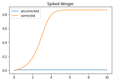
Figure 1. The cosine similarity in the spiked matrix problem with Rademacher latent variable and noise with mean $1$ solved using corrected and uncorrected least squares. A data matrix of size $2500\times 2500$ and the uncorrected and corrected likelihoods were optimized using gradient descent. The plot displays the cosine similarity plotted against the number of steps. It is clear that correcting the likelihood gets rid of the effect from the score parameter, and the corresponding pseudo maximum likelihood estimator achieves a non-zero cosine similiarty.

5.2. Stochastic Block Model

We now consider a community detection problem with two groups. We work with the stochastic block model SBM$(n,\frac{1}{2}+\mu_{0}N^{-1/2},\frac{1}{2}-\mu_{0}N^{-1/2})$ on two communities. In this model we shall assume that our unknown signal $\bm{x}^{0}$ lies in $\{\pm 1\}^{N}$, and serves as the index vector for the two communities. The corresponding data matrix is the adjacency matrix, and its entries have distribution given by:

$$\operatorname{\mathbb{P}}\left(Y_{i,j}=1\>|\>\frac{x_{i}x_{j}}{\sqrt{N}}\right)=\frac{1}{2}+\mu_{0}\frac{x_{i}x_{j}}{\sqrt{N}}\ \quad\text{ and }\quad\operatorname{\mathbb{P}}\left(Y_{i,j}=0\>|\>\frac{x_{i}x_{j}}{\sqrt{N}}\right)=\frac{1}{2}-\mu_{0}\frac{x_{i}x_{j}}{\sqrt{N}}\,.$$

The parameter $\mu_{0}>0$ represents the difference between the probability of edges appearing within and outside of each group. Notice that when $x_{i},x_{j}$ take the same sign, the probability is higher, and when $x_{i}x_{j}$ take different signs then the probability of connecting an edge is lower. The $\sqrt{N}$ scaling is such that the detection problem becomes non-trivial, and a phase transition on the weak recovery of the groups is observable (see  [60] ). More generally the Stochastic block model has been studied in a wide variety of regimes for the connection probabilities between communities (see  [1] for a detailed overview of different regimes). There is a large collection of literature concerned with showing when different notions of recovery of the communities is possible, as well as when there are efficient algorithms for recovery. See  [2, 43, 66, 42, 63, 27] and the references therein.
For the SBM with connection probabilities as above, the loglikelihood is given by

$$g_{0}(Y,w)=Y\ln(\frac{1}{2}+\mu_{0}w)+(1-Y)\ln(\frac{1}{2}-\mu_{0}w).$$

Suppose that a signal to noise ratio $\mu_{0}\neq\mu$ is chosen, that is, we choose the pseudo-likelihood

$$g(Y,w)=Y\ln(\frac{1}{2}+\mu w)+(1-Y)\ln(\frac{1}{2}-\mu w)\,,$$

then the information parameters are given by

$$\beta_{1}=4\mu^{2},\beta_{2}=4\mu\mu_{0},\beta_{3}=4\mu^{2},\beta_{4}=0\,,$$

and the Rao relation is not satisfied. We note however that $\beta_{4}=0$ and so our choice of pseudo-likelihood is well scored.

One method to introduce an ill-scored pseudo-likelihood is to work with an incorrect assumption on the null-model. If we suppose that null model corresponds to the adjacency matrix of a $G(n,p)$ matrix with $p\neq 1/2$, that is the pseudo-likelihood is given by:

$$g_{p}(y,w)=y\log(p+\mu w)+(1-y)\log(1-p-\mu w)\,,$$

and a direct computation yields:

$$\beta_{4}^{g_{p}}=\frac{\mu(1-2p)}{2p(1-p)}\,,$$

which is zero if and only if $p=1/2$.

5.3. Sparse Rademacher Matrices and Best Rank-1 approximation

We now consider a class of sparse submatrix detection problems [16]. For this example, we suppose that our unknown vector lies in $\Omega^{N}$ where $\Omega$ is either an interval $[a,b]$ or a finite set.
Consider the case where $Y$ is a sparse Rademacher matrix, i.e $Y$, conditionally on $w$, takes values in $\{-1,0,1\}$ with probabilities given by:

$$\operatorname{\mathbb{P}}\Big{(}Y_{ij}=\pm 1|\frac{x_{i}x_{j}}{\sqrt{N}}\Big{)}=\frac{p}{2}+\lambda\frac{x_{i}x_{j}}{\sqrt{N}}\,,\qquad\text{and}\qquad\operatorname{\mathbb{P}}\Big{(}Y=0|\ \frac{x_{i}x_{j}}{\sqrt{N}}\Big{)}=1-p-2\lambda\frac{x_{i}x_{j}}{\sqrt{N}}\,,$$ (5.3)

where throughout $p$ is a fixed number in $(0,1)$. In this case the log-likelihood is given by:

$$g_{0}(Y,w)=(1-Y^{2})\log(1-p-2\lambda w)+\frac{Y(Y-1)}{2}\log\Big{(}\frac{p}{2}+\lambda w\Big{)}-\frac{Y(1+Y)}{2}\log\Big{(}\frac{p}{2}+\lambda w\Big{)}\,,$$

and the corresponding score parameters are given by:

$$\beta_{1}=\beta_{2}=\beta_{3}=\frac{4\lambda^{2}}{1-p}+\frac{\lambda^{2}}{p}\,.$$

Suppose now that we try to infer the unknown vector via the best rank 1 approximation, that is, we try to minimize

$$\min_{x\in{\Omega}^{N}}\left\lVert Y-\lambda\frac{\bm{\mathbf{x}}\bm{\mathbf{x}}^{T}}{\sqrt{N}}\right\rVert_{F}^{2}\,,$$

then as discussed in Section  4, the corresponding estimator $\bm{\mathbf{x}}_{LS}$ corresponds to a pseudo likelihood estimator $\hat{}\bm{\mathbf{x}}_{\mathrm{PMLE}}$ with pseudo-likelihood given by:

$$g(Y,w)=-\frac{1}{2}(Y-\lambda w)^{2}-\log(2\pi)\,.$$

By Proposition  4.1 the model is well scored, and furthermore, an explicit computation shows the Fisher parameters for the gaussian equivalent are given by:

$$\beta_{1}=\lambda p,\beta_{2}=0,\beta_{3}=\lambda^{2}\,,$$

and consequently by Proposition 4.2 the least-square estimator is completely uninformative provided that the limiting empirical measure of $\bm{\mathbf{x}}^{0,N}$ is balanced.

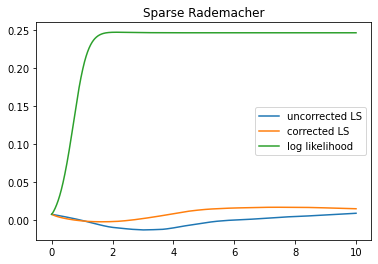
Figure 2. The cosine similarity in the sparse Rademacher problem for corrected and uncorrected least squares, and the log-likelihood. A data matrix of size $2500\times 2500$ was used, and corrected and uncorrected least squares was performed on the data matrix and optimized using gradient descent. The plot displays the cosine similarity plotted against the number of steps. It is clear that the least squares estimator was uninformative and always achieved a cosine-similarity of zero. However, when gradient descent was performed on the log-likelihood, we see that maximum likelihood estimator achieved non-trivial performance. This demonstrates the failure of least squares in some problems that can be solvable by MLE.

5.4. Non-Linear transformations of rank $1$ matrices

Consider a data vector $x\in\{\pm 1\}^{N}$, and a spiked Wigner matrix $W$ given by:

$$W=G+\frac{\lambda}{\sqrt{N}}xx^{T}\,,$$

where $G$ is a symmetric matrix with i.i.d standard Gaussian entries. From $W$ we consider the transformation taking each entry $W_{ij}$ and sending them to $Y_{ij}=F(W_{ij})$ for some function $F$. Non-linear transformations of random matrices have applications in to kernel methods [79, 55, 54] and the spectra of one-layer neural networks [73, 75, 22]. The spectra of $F(W_{ij})$ was thoroughly analyzed in [39] and [33].

From the matrix $Y$ we will study the behavior of maximum likelihood estimation for certain choices of $F$. We remark that some choices of $F$ will lead to irregular likelihoods that do not fall into our framework. We provide an example in Section  5.4.2.

5.4.1. Rounded Entries:

Suppose that $F(x)=\text{sgn}(x)$ (with the convention that $\text{sgn}(0)=1$). This is the censored spiked matrix model that was studied recently in [57]. In this case the likelihood of the output matrix $Y$ is given by:

$$g(y,w)=\frac{(1-y)}{2}\log\frac{1}{\sqrt{2\pi}}\int_{-\infty}^{-\lambda w}e^{-\frac{x^{2}}{2}}dx+\frac{(1+y)}{2}\log\frac{1}{\sqrt{2\pi}}\int_{-\lambda w}^{\infty}e^{-x^{2}/2}dx\,.$$

We may explicitly compute the $\beta$ values in this case:

$$\beta_{1}=\beta_{2}=\beta_{3}=\frac{2}{\pi}\lambda^{2},\beta_{4}=0\,.$$

5.4.2. Squaring Entries:

We now provide an example which does not fall into the class $\mathcal{F}_{0}$. Suppose we choose $F(x)=x^{2}$, then explicitly one computes the log-likelihood to be given by:

$$g(y,w)=-\frac{1}{2}\log(2\pi)-\log(2)-\frac{1}{2}\log(y)+\log\left[e^{-(\sqrt{y}-\lambda w)^{2}/2}+e^{-(\sqrt{y}+\lambda w)^{2}/2}\right]\,.$$

In particular, the second derivative of $g(y,w)$ at $w=0$ is given by:

$$\partial_{w}^{2}g(y,0)=\lambda^{2}(y-1)\,,$$

and consequently the bound $\left\lVert\partial_{w}^{2}g(\cdot,0)\right\rVert<\infty$ fails.

6. Outline of Proofs

In this section, we will summarize the strategy to prove the main results. The proofs will be deferred to the relevant sections of the Appendix. To simplify the notation in this section, we only consider the ill-scored scenario. The case for well-scored problems are simpler and the proof is essentially the same. The only difference is the constraint on the mean $\bar{x}$, which is unneeded.

6.1. Universality

We begin by showing that the limit of the (normalized) maximum pseudo-likelihood is equivalent to that obtained by a maximization of a Gaussian model parameterized by the information parameters. The Gaussian model is given by

$$H_{N}^{\bar{\beta}}(x) =\frac{\sqrt{\beta_{1}}}{\sqrt{N}}\sum_{1\leq i\leq j\leq N}g_{ij}x_{i}x_{j}+\frac{\beta_{2}}{N}\sum_{1\leq i\leq j\leq N}x_{i}^{0}x_{j}^{0}x_{i}x_{j}-\frac{\beta_{3}}{2N}\sum_{1\leq i\leq j\leq N}x_{i}^{2}x_{j}^{2}+\beta_{4}\sum_{1\leq i\leq j\leq N}\frac{x_{i}x_{j}}{\sqrt{N}}\,$$

$$=\frac{\sqrt{\beta_{1}}}{\sqrt{N}}\sum_{ij}g_{ij}x_{i}x_{j}+\frac{N\beta_{2}}{2}M_{N}(x)^{2}-\frac{N\beta_{3}}{4}S_{N}(x)^{2}+\beta_{4}N^{\frac{3}{2}}(\bar{x})^{2}+O(1)\,$$ (6.1)

where we recall that $M_{N}$ and $S_{N}$ denote the normalized inner product and norm defined in (2.14) and $\bar{x}=\frac{1}{N}\sum_{i=1}^{N}x_{i}$ is the sample mean.

We prove in Appendix A that the asymptotic maxmium pseudolikelihood is equal to the one given by the maximum of the gaussian equivalent on average. Given $S,M,v\subseteq\mathbb{R}$, recall that $\Omega_{\varepsilon}(S,M,v)$ defined in (2.16) denotes the set of points in $\Omega^{N}$ within $\varepsilon$ of $(S,M,v)$ and let us define

$$\mathcal{L}_{N}^{g,\varepsilon}(S,M,v) =\mathbb{E}\max_{\Omega_{\varepsilon}(S,M,v)}\bigg{(}\sum_{i<j}g\Big{(}Y_{ij},\frac{x_{i}x_{j}}{\sqrt{N}}\Big{)}-\sum_{i<j}g(Y_{ij},0)\bigg{)}\,,$$ (6.2)

$$\mathcal{L}_{N}^{\bar{\beta},\varepsilon}(S,M,v) =\mathbb{E}\max_{\Omega_{\varepsilon}(S,M,v)}H_{N}^{\bar{\beta}}(x)\,,$$ (6.3)

to denote the restricted pseudo likelihood and the gaussian likelihood respectively. We prove in Appendix A that the pseudo maximum likelihood and the maximum of the Gaussian equivalent are asymptotically equal in the following sense.

Lemma 6.1.

If $g,g_{0}\in\mathcal{F}_{0}$, then for any $(S,M,v)\in\mathcal{C}_{c}$

$$\lim_{N\to\infty}\frac{1}{N}|\mathcal{L}_{N}^{g,\varepsilon}(S,M,v)-\mathcal{L}_{N}^{\bar{\beta},\varepsilon}(S,M,v)|=0\,,$$

This is proved by showing equivalence for smooth approximations of the maximum likelihood. Let $\operatorname{\mathbb{P}}_{X}(x)$ be the uniform measure on $\Omega$. We approximate the pseudo maximum likelihood with log likelihood ratio of the posterior. We define the log-likelihood ratio associated with the pseudo likelihood

$$F_{N}(g,\varepsilon;S,M,v):=\frac{1}{N}\bigg{(}\mathbb{E}_{Y}\Big{(}\log\int_{\Omega_{\varepsilon}(S,M,v)}e^{\sum_{i<j}g\Big{(}Y_{ij},\frac{x_{i}x_{j}}{\sqrt{N}}\Big{)}}\,d\operatorname{\mathbb{P}}_{X}^{\otimes N}(\bm{\mathbf{x}})-\sum_{i<j}g(Y_{ij},0)\Big{)}\bigg{)}\,,$$ (6.4)

where $\mathbb{E}_{Y}$ is with the expectation with respect to the conditional data distribution (2.1). On the other hand, we define the log-likelihood ratio of the Gaussian equivalent for $\bar{\beta}=(\beta_{1},\beta_{2},\beta_{3},\beta_{4})\in\mathbb{R}^{4}$ by

$$F_{N}(\bar{\beta},\varepsilon;S,M,v):=\frac{1}{N}\mathbb{E}_{Y}\log\int_{\Omega_{\varepsilon}(S,M,v)}e^{H_{N}^{\bar{\beta}}(\bm{\mathbf{x}})}\,d\operatorname{\mathbb{P}}_{X}^{\otimes N}(\bm{\mathbf{x}})\,,$$ (6.5)

where $H_{N}^{\bar{\beta}}(\bm{\mathbf{x}})$ is as in (6.1). We define $F_{N}^{g,\varepsilon}$ and $F_{N}^{\bar{\beta},\varepsilon}$ to be the equal to (6.4) and (6.5) without the constraints in the integrand. These quantities approximate the pseudo maximum likelihood in the sense that for any $(S,M,v)\in\mathcal{C}_{c}$

$$\lim_{L\to\infty}\lim_{N\to\infty}|\frac{1}{L}F_{N}(Lg,\varepsilon;S,M,v)-\frac{1}{N}\mathcal{L}_{N}^{g,\varepsilon}(S,M,v)| =0$$ (6.6)

$$\lim_{L\to\infty}\lim_{N\to\infty}|\frac{1}{L}F_{N}(L\bar{\beta},\varepsilon;S,M,v)-\frac{1}{N}\mathcal{L}_{N}^{\bar{\beta},\varepsilon}(S,M,v)| =0\,.$$ (6.7)

An analogous statement holds for the unconstrained versions. Universality for the pseudo maximum likelihood in Lemma 6.1 follows from the following universality for the log-likelihood functions:

Lemma 6.2.

If $g,g_{0}\in\mathcal{F}_{0}$, then for any $S,M,v\in\mathcal{C}_{c}$

$$\lim_{L\to\infty}\lim_{N\to\infty}\bigg{|}\frac{1}{L}F_{N}(Lg,\varepsilon;S,M,v)-\frac{1}{L}F_{N}(L\bar{\beta},\varepsilon;S,M,v)\bigg{|} =0$$

$$\lim_{L\to\infty}\lim_{N\to\infty}\bigg{|}\frac{1}{L}F_{N}^{Lg,\varepsilon}-\frac{1}{L}F_{N}^{L\bar{\beta},\varepsilon}\bigg{|} =0$$

Proof sketch.

The proof follows the arguments in [40, Section 3]. The key difference is that the universality result is extended to ill-scored models. The technical details of this argument are provided in Appendix A for generic constraints, but we identify the key steps below.

The key idea in this proof is that at the level of the log likelihood, we are able to use Taylor’s theorem to expand around the likelihood in the exponent with respect to $\frac{x_{i}x_{j}}{\sqrt{N}}$,

$$\frac{1}{L}F_{N}(Lg,\varepsilon;S,M,v)=\frac{1}{NL}\mathbb{E}_{Y}\Big{(}\log\int_{\Omega_{\varepsilon}(S,M,v)}e^{\sum_{i<j}\partial_{w}Lg(Y_{ij},0)w_{ij}+\frac{1}{2}\partial_{w}^{(2)}Lg(Y_{ij},0)w_{ij}^{2}}\,d\operatorname{\mathbb{P}}_{X}^{\otimes N}(\bm{\mathbf{x}})\Big{)}+o_{N}(1)\,$$

since the third derivative of $g$ is uniformly bounded for $g\in\mathcal{F}_{0}$. The second order coefficients of the Taylor series will concentrate in the high-dimensional limit while the first order term will be approximately Gaussian with a specific mean and variance given by,

$$\mathbb{E}[\partial_{w}g(Y_{ij},0)]=\beta_{4}+\frac{x_{i}^{0}x_{j}^{0}}{\sqrt{N}}\beta_{2}+O(N^{-1})\quad\text{ and }\quad\operatorname{Var}[\partial_{w}g(Y_{ij},0)]=\beta_{1}+O(N^{-1/2}).$$

The decomposition then follows immediately from standard universality in disorder arguments for spin glasses, see, e.g., [18]. We conclude that

$$\lim_{L\to\infty}\lim_{N\to\infty}\bigg{|}\frac{1}{L}F_{N}(Lg,\varepsilon;S,M,v)-\frac{1}{L}F_{N}(L\bar{\beta},\varepsilon;S,M,v)\bigg{|}=0.$$

The proof for the unconstrained problem is identical. ∎

The proof of Lemma 6.1 now follows from the triangle inequality.

Proof of Lemma 6.1.

By the triangle inequality, we have

$$\frac{1}{N}|\mathcal{L}_{N}^{g,\varepsilon}(S,M,v)-\mathcal{L}_{N}^{\bar{\beta},\varepsilon}(S,M,v)| \leq|\frac{1}{N}\mathcal{L}_{N}^{g,\varepsilon}(S,M,v)-\frac{1}{L}F_{N}(Lg,\varepsilon;S,M,v)|$$

$$\quad+\bigg{|}\frac{1}{L}F_{N}(Lg,\varepsilon;S,M,v)-\frac{1}{L}F_{N}(L\bar{\beta},\varepsilon;S,M,v)\bigg{|}$$

$$\quad+|\frac{1}{L}F_{N}(L\bar{\beta},\varepsilon;S,M,v)-\frac{1}{N}\mathcal{L}_{N}^{\bar{\beta},\varepsilon}(S,M,v)|\,.$$

The first and third terms vanish in the limit by (6.6) and the second term vanishes by Lemma 6.2. ∎

The main consequence of Lemma 6.2 is that it suffices to compute the limit in the case of the Gaussian equivalent of $F_{N}(\bar{\beta};S,M,v)$ instead of the pseudo maximum likelihood. The computation of this limit is the focus of the following two sections.

6.2. Derivation of the Variational Formula I

In this section, we once again use the approximation of the likelihoods with the loglikelihood ratios and first compute the limit of the loglikelihood ratio. Our goal is to first define the variational formula for the loglikelihood ratios.

Notice that the term corresponding to $H_{N}^{\bar{\beta}}$ is of higher order, so this term must be corrected in order to have a well-defined limit. To this end, we define

$$H_{N}^{\bar{\beta},\alpha}(\bm{\mathbf{x}})=H_{N}^{\bar{\beta}}(\bm{\mathbf{x}})-\beta_{4}N^{\frac{3}{2}}(\bar{x})^{2}+\alpha N(\bar{x})^{2}\,,$$ (6.8)

which is the gaussian equivalent for (2.21). We define

$$F_{N,\alpha}(\bar{\beta},\alpha,\varepsilon;S,M,v):=\frac{1}{N}\mathbb{E}_{Y}\log\int_{\Omega_{\varepsilon}(S,M,v)}e^{H_{N}^{\bar{\beta},\alpha}(\bm{\mathbf{x}})}\,d\operatorname{\mathbb{P}}_{X}^{\otimes N}(\bm{\mathbf{x}})\,,$$ (6.9)

and let $F_{N,\alpha}(\bar{\beta},\alpha,\varepsilon)$ denotes its unconstrained version.

We now define the variational formula which will compute the limit. Let $\zeta$ be a probability measure, and let $\Phi_{\zeta,\mu,\lambda,\rho}(t,y)$ be the unique weak solution to the Parisi PDE

$$\begin{cases}\partial_{t}\Phi_{\zeta,\mu,\lambda,\rho}=-\frac{\beta_{1}}{4}(\partial_{y}^{2}\Phi_{\zeta}+\zeta([0,t])(\partial_{y}\Phi_{\zeta})^{2})&(t,y)\in(0,S)\times\mathbb{R}\\ \Phi_{\zeta,\mu,\lambda,\rho}(S,y;)=\log\int e^{yx+\lambda xx^{0}+\mu x^{2}+\rho x}\,d\operatorname{\mathbb{P}}_{X}(x)\end{cases}\,.$$ (6.10)

See [49] for the notion of weak solutions for this PDE and the corresponding well-posedness. Define the corresponding Parisi functional by

$$\varphi_{\bar{\beta},\alpha}(S,M,v)$$ (6.11)

$$=\inf_{\mu,\lambda,\rho,\zeta}\bigg{(}\mathbb{E}_{x^{0}\sim\operatorname{\mathbb{Q}}}[\Phi_{\zeta,\mu,\lambda,\rho}(0,0)]-\frac{\beta_{1}}{2}\int_{0}^{S}t\zeta([0,t])\,dt-\mu S-\lambda M-\rho v+\frac{\beta_{2}M^{2}}{2}-\frac{\beta_{3}S^{2}}{4}+\frac{\alpha v^{2}}{2}\bigg{)}\,.$$

Furthermore, we see that $(S_{N}(\bm{\mathbf{x}}_{\mathrm{PMLE}}),M_{N}(\bm{\mathbf{x}}_{\mathrm{PMLE}}),\bar{}\bm{\mathbf{x}}_{\mathrm{PMLE}})$ asymptotically live in the closed subset $\mathcal{C}_{c}$ of $[0,C^{2}]\times[-C^{2},C^{2}]\times[-C,C]$ defined in (2.12). This is the domain of our functional. We will show in Appendix B that the limit of the loglikelihood is given by the Parisi functional.

Theorem 6.1.

For any $\beta_{1},\beta_{2},\beta_{3}$ and $\alpha$ and constraints $(S,M,v)\in\mathcal{C}$, we have

$$\lim_{\varepsilon\to 0}\lim_{N\to\infty}F_{N,\alpha}(\bar{\beta},\alpha,\varepsilon;S,M,v) =\varphi_{\mathbf{\beta},\alpha}(S,M,v)$$

$$\lim_{\varepsilon\to 0}\lim_{N\to\infty}F_{N,\alpha}(\bar{\beta},\alpha,\varepsilon) =\sup_{(S,M,v)\in\mathcal{C}}\varphi_{\mathbf{\beta},\alpha}(S,M,v).$$

Remark 6.1.

For regular models, the constraint on $v$ can be completely removed and was proven in [40]. In such cases, the optimization is over the functional $\varphi_{\bar{\beta}}$ which is defined on only two parameters $S$ and $M$.

Proof sketch of Theorem 6.1.

The proof of this results use techniques first developed to study mean-field models of spin glasses. By introducing a small perturbation to the log-likelihood, we are able to characterize the limiting behaviour of independent samples from the perturbed posterior measure and explicitly compute the limit. The proof also borrows techniques from large deviations to remove the constraint on the overlaps. We sketch the key steps.

Upper Bound: We first prove that

$$F_{N,\alpha}(\bar{\beta},\alpha,\varepsilon;S,M,v)\leq\varphi_{\mathbf{\beta},\alpha}(S,M,v).$$ (6.12)

This argument follows from a Guerra-type replica symmetry breaking interpolation [38]. In particular, it follows from the computations in Proposition B.1 that for any $\lambda,\mu,\rho$ and $\zeta$

$$F_{N,\alpha}(\bar{\beta},\alpha,\varepsilon;S,M,v) \leq-\lambda S-\mu M-\rho v+\frac{1}{N}\sum_{i=1}^{N}\Phi_{\lambda,\mu,\zeta}(0,0)-\frac{\beta_{1}^{2}}{2}\int_{0}^{S}t\zeta(t)\,dt$$

$$+\frac{\beta_{2}}{2}M^{2}-\frac{\beta_{3}}{4}S^{2}+\frac{\alpha}{2}v^{2}+L\varepsilon(|\mu|+|\lambda|+|\rho|)+o_{N,\varepsilon}(1)\,$$

This upper bound holds for all $\lambda,\mu,\rho$ and $\zeta$, so we can take the infumum to arrive at (6.12). The sharpness of the upper bound after minimizing over $\lambda,\mu,\rho$ is a consequence of a modification of the Gartner–Ellis Theorem [25, Theorem 2.3.6] and is given in detail in Lemma B.1.

Lower Bound: We then prove the matching lower bound

$$F_{N,\alpha}(\bar{\beta},\alpha,\varepsilon;S,M,v)\geq\varphi_{\mathbf{\beta},\alpha}(S,M,v).$$

This proof uses the cavity method, in this case called the Aizenman-Sims-Star scheme [4], and a perturbation of the posterior that forces the limiting overlap to satisfy the Ghirlanda–Guerra identities [36] and ultrametricity [68]. The proof of the lower bound is included in Proposition B.2 for completeness. It is worth pointing out that on the set $\Omega_{\varepsilon}(S,M,v)$, the $S_{N}(\bm{\mathbf{x}})$ is approximately constant, so we can do a change of variables restrict ourselves onto the ball of radius $S$ at the cost of a small error term, which we can control. This implies that the usual proof of the Ghirlanda–Guerra identities holds directly in our setting. ∎

Having computed the appropriate limit of $F_{N}(\bar{\beta};S,M,v)$, we can apply Lemma 6.2 to recover the limit of the loglikihood ratio. By (6.6) if one can compute the limit of this quantity as $L\to\infty$, then we can recover the limiting formula for the pseudo maximum likelihood.

6.3. Derivation of the Variational Formula II

This variational formula holds for all $\beta_{1},\beta_{2},\beta_{3}$ and $\alpha$, so it also holds when these parameters are scaled by $L$ as in the smooth approximation. We will show in Appendix C that taking the limit as $L\to\infty$ of this variational formula will give the formula for the pseudo maximum likelihood, after an application of (6.6), which will give us a variational formula for the limit of pseudo maximum likelihood.

Lemma 6.3.

For any $\bar{\beta}$, in the constrained pseudo maximum likelihood we have

$$\lim_{\varepsilon\to 0}\lim_{N\to\infty}\frac{1}{N}\mathcal{L}_{N,\alpha}^{g,\varepsilon}(S,M,v) =\lim_{\varepsilon\to 0}\lim_{N\to\infty}\frac{1}{N}\mathcal{L}_{N}^{\bar{\beta},\varepsilon}(S,M,v)=\psi_{\bar{\beta},\alpha}(S,M,v)\,$$

$$\lim_{\varepsilon\to 0}\lim_{N\to\infty}\frac{1}{N}\mathcal{L}_{N}^{g,\varepsilon} =\lim_{\varepsilon\to 0}\lim_{N\to\infty}\frac{1}{N}\mathcal{L}_{N,\alpha}^{\bar{\beta},\varepsilon}=\sup_{(S,M,v)\in\mathcal{C}_{c}}\psi_{\bar{\beta},\alpha}(S,M,v)\,,$$

where $\psi_{\bar{\beta},\alpha}$ is as in (2.23)

This proof uses the $\Gamma$ limit of the solutions in [48] to the Parisi PDE (B.19) to identify $\psi_{\bar{\beta}}$ as the limit of $\frac{1}{L}\varphi_{\bar{\beta}}$. In the lemma above the constrained case is established in Appendix  C. The limit formula in the unconstrained is established in Appendix  D.

Having understood the limiting variational formula, one can also show using (6.6), that this limiting variational formula characterizes the constrained pseudo maximum likelihood.

We can conclude that the limit of the pseudo maximum likelihood is a variational optimization over the parameters $S,M,v$. We will show in the next section that the maximizers of the variational problem encode the limiting performance of the maximum likelihood estimators.

6.4. Characterization of the Maximizers

In Appendix F we prove tightness of the overlaps as stated in Theorems  2.1 and  2.5. The tightness will follow from concentration properties satisfied by the gaussian equivalent  (6.1), and the results proved in Appendix  C.

Next, under the further assumption that $\psi_{\bar{\beta},\alpha}$ has a unique maximizer, we are able to prove the following characterization of performance:

Lemma 6.4.

For $g,g^{0}\in\mathcal{F}_{0}$ let $\bar{\beta}$ denote the corresponding information and score parameters and suppose that $\psi_{\bar{\beta}}$ has a unique (up to the sign of $m$) maximizer $(s_{\bar{\beta}},\pm m_{\bar{\beta}},v_{\bar{\beta}})$. Then

$$|\mathbf{CS}(\hat{\mathbf{x}}_{\mathrm{PMLE}},\mathbf{x}_{0})| \to\frac{|m_{\bar{\beta}}|}{(s_{\bar{\beta}}\mathbb{E}_{\mathbb{Q}}(x^{0})^{2})^{1/2}}\qquad\,\text{a.s}$$ (6.13)

$$\frac{1}{N}\left\lVert\hat{x}_{PMLE}\right\rVert^{2} \to s_{\bar{\beta}}\qquad\,\text{a.s.}$$ (6.14)

Proof sketch.

The proof follows from the fact that the limit of the constrained pseudo maximum likelihood over the set $\Omega_{\varepsilon}(s,m,v)$ is given by $\psi_{\bar{\beta}}(s,m,v)$,

$$\lim_{\varepsilon\to 0}\lim_{N\to\infty}\frac{1}{N}\mathbb{E}\max_{\Omega_{\varepsilon}(s,m)}H_{N}^{\bar{\beta}}(\bm{\mathbf{x}})=\psi_{\bar{\beta}}(s,m)$$ (6.15)

which follows from Lemma 6.3. In the notation above, we have defined

$$\psi_{\bar{\beta}}(S,M)=\begin{cases}\sup_{v}\psi_{\bar{\beta},\alpha}(S,M,v)&\text{ if }\alpha\neq 0\\ \psi_{\bar{\beta},0}(S,M)&\text{ if }\alpha=0.\end{cases}$$

to handle the cases for well-scored and corrected models simultaneously. Next, by concentration [3, Section 2.1] for every $\varepsilon>0$,

$$\lim_{N\to\infty}\frac{1}{N}\mathbb{E}\max_{x\in\Omega^{N}}H_{N}^{\bar{\beta}}(\bm{\mathbf{x}})=\lim_{N\to\infty}\frac{1}{N}\mathbb{E}\max_{s,m}\max_{\Omega_{\varepsilon}(s,m)}H_{N}^{\bar{\beta}}(\bm{\mathbf{x}})=\lim_{N\to\infty}\frac{1}{N}\max_{s,m}\mathbb{E}\max_{\Omega_{\varepsilon}(s,m)}H_{N}^{\bar{\beta}}(\bm{\mathbf{x}})\,.$$

Since the maximizer $(s_{\bar{\beta}},\pm m_{\bar{\beta}},v_{\bar{\beta}})$ is unique up to a sign and $H_{N}^{\bar{\beta}}$ only depends on $S_{N}$ and $M_{N}$ through its squared value we have

$$\lim_{N\to\infty}\frac{1}{N}\mathbb{E}\max_{x\in\Omega^{N}}H_{N}^{\bar{\beta}}(\bm{\mathbf{x}})=\lim_{N\to\infty}\frac{1}{N}\mathbb{E}\max_{s,m}\max_{\Omega_{\varepsilon}(s,m)}H_{N}^{\bar{\beta}}(\bm{\mathbf{x}})=\lim_{N\to\infty}\frac{1}{N}\mathbb{E}\max_{\Omega_{\varepsilon}(s_{\bar{\beta}},m_{\bar{\beta}})}H_{N}^{\bar{\beta}}(\bm{\mathbf{x}})\,.$$

Finally, we can apply universality in Lemma 6.1 to conclude that the pseudo maximum likelihood is maximized on the set $\Omega_{\varepsilon}(s_{\bar{\beta}},m_{\bar{\beta}})$, which implies that the PMLE satisfies

$$|M_{N}(\bm{\mathbf{\hat{x}}}^{g}_{\mathrm{PMLE}})|=|M_{N}(\bm{\mathbf{\hat{x}}}^{\bar{\beta}}_{\mathrm{PMLE}})|=|m_{\bar{\beta}}|\quad\text{ and }\quad S_{N}(\bm{\mathbf{\hat{x}}}^{g}_{\mathrm{PMLE}})=S_{N}(\bm{\mathbf{\hat{x}}}^{\bar{\beta}}_{\mathrm{PMLE}})=s_{\bar{\beta}}$$

leading to the characterization of the cosine similarity and norm. ∎

If the maximizers of $\psi_{\bar{\beta}}$ are not unique, then the limit points of all near maximizers are attained on the set $\mathcal{C}_{\bar{\beta}}$ or $\mathcal{C}_{\bar{\beta},\alpha}$

Lemma 6.5.

Let $\overline{\beta}$ be fixed, and suppose that $(S,M)$ are such that $-\infty<\psi(S,M)<\sup\psi$. Let $\text{GS}_{N}$ denote the (random) collection of maximizers of $H_{N}^{\overline{\beta}}$ in $\Omega^{N}$, then for $\varepsilon>0$ sufficiently small, one has:

$$\varlimsup_{N\to\infty}\frac{1}{N}\log\operatorname{\mathbb{P}}(\text{GS}_{N}\cap\{\bm{\mathbf{x}}\mathrel{}\mid\mathrel{}S_{N}(\bm{\mathbf{x}})\approx_{\varepsilon}S,M_{N}(\bm{\mathbf{x}})\approx_{\varepsilon}M\}\neq\emptyset)<0\,.$$

Furthermore, one has that the collection of all limit points, taken over all sequences of near maximizers $\bm{\mathbf{x}}_{N}$, for the sequence $(S_{N}(\bm{\mathbf{x}}),M_{N}(\bm{\mathbf{x}}))$ is equal to $\mathcal{C}_{\bar{\beta}}$.

Proof sketch.

The detailed proof of this argument is deferred to Lemma 6.5. It essentially follows a similar line of reasoning as Lemma 6.4 and relies on the characterization of pseudo maximum likelihood in (6.15) and the exponential concentration of $H_{N}^{\bar{\beta}}$ to achieve an exponential rate of concentration of the event. ∎

The two preceding Lemmas provide the characterization of the cosine simlarity in Theorems  2.1 and  2.5.

6.5. Coarse Equivalence of Estimators

In Section G, we will provide a detailed prove a sufficient condition for when two likelihoods are coarsely equivalent. Coarse equivalence will follow as a consequence of the universality result in Lemma 6.1.

Proof of Theorem 3.2 and Theorem 3.3.

We first provide a proof of Theorem 3.3. We start with the first condition in Theorem 3.3. Given likelihoods $g^{1},g^{2}$ which satisfy :

$$\frac{\sqrt{\beta_{1}(g^{1})}}{\sqrt{\beta_{1}(g^{2})}}=\frac{\beta_{2}(g^{1})}{\beta_{2}(g^{2})}=\frac{\beta_{3}(g^{1})}{\beta_{3}(g^{2})}=\frac{\beta_{4}(g^{1})}{\beta_{4}(g^{2})}=C,$$ (6.16)

the corresponding gaussian equivalents will be a scalar multiple of each-other. Consequently the collection of near-maximizers will be the same for both problems, and the result will then follow from Theorem 2.1.

To see the second statement, notice that if our parameter space satisfies $|x|=C$, then the maximizer of the gaussian equivalent $H_{N}^{\bar{\beta}}$ given in (6.1) is independent of $\beta_{3}$ since it is constant, which proves the second statement in Theorem 3.3.

The proof of Theorem 3.2 will follow from a a similar argument, where we appeal to Theorem 2.1. ∎

We further prove Theorem  3.1 in this section, it will be an immediate consequence of the universality established in Theorems  2.1 and  2.5.

Proof of Theorem 3.1.

It suffices to show that the information parameters of $(g_{U,0}^{\bar{\beta}},g_{U,1}^{\bar{\beta}})$ are equal to $\bar{\beta}$. We have

$$\partial_{w}g_{U,0}^{\bar{\beta}}(y,0)=\frac{\beta_{2}}{\beta_{1}}(y-\beta_{4}),\quad\partial_{w}g_{U,1}^{\bar{\beta}}(y,0)=y,\quad\partial_{w}^{2}g_{U,1}^{\bar{\beta}}(y,0)=\beta_{3}.$$

Furthermore, under the null-model we have that $Y$ is Gaussian with mean $\beta_{4}$ and variance $\beta_{1}$. A direct computation implies that the information parameters of $(g_{U,0}^{\bar{\beta}},g_{U,1}^{\bar{\beta}})$ are $\beta_{1},\beta_{2},\beta_{3},\beta_{4}$.

∎

Acknowledgements

C.G. acknowledges the partial support of the Natural Sciences and Engineering Research Council of Canada Post-Graduate Scholarship Doctoral award. A.J. and J.K. acknowledge the support of the Natural Sciences and Engineering Research Council of Canada (NSERC), the Canada Research Chairs programme, and the Ontario Research Fund. Cette recherche a été enterprise grâce, en partie, au soutien financier du Conseil de Recherches en Sciences Naturelles et en Génie du Canada (CRSNG), [RGPIN-2020-04597, DGECR-2020-00199], et du Programme des chaires de recherche du Canada.

Appendix A Universality with Non-Zero Score

In this section, we prove universality of pseudo maximum likelihood estimation with possibly non-zero score parameters. This extends the universality result in [40] to the case of the pseudo maximum likelihood and removes the zero score assumption in [40, Hypothesis 2.3].

Given the information parameters, $\bar{\beta}$, we recall the gaussian equivalent $H^{\bar{\beta}}_{N}$ from (6.1) Likewise, given $S,M,v$ recall that $\mathcal{L}_{N}^{g,\varepsilon}(S,M,v)$ and $\mathcal{L}_{N}^{\bar{\beta},\varepsilon}(S,M,v)$ denotes the normalized pseudo maximum likelihood and the maximum of the gaussian equivalent respectively. The goal of this section is to show that these quantities converge to the same value as stated in Lemma 6.1,

$$\lim_{N\to\infty}\frac{1}{N}|\mathcal{L}_{N}^{g,\varepsilon}(S,M,v)-\mathcal{L}_{N}^{\bar{\beta},\varepsilon}(S,M,v)|=0\,.$$

The proof of the maximum likelihood formulas will follow from an extension of the universality for Bayesian models proven in [40]. In contrast to the Bayesian inference setting, we fix $\bm{\mathbf{x}}^{0}$ and define the log-likelihood ratios

$$F_{N}(g;S,M,v)=\frac{1}{N}\bigg{(}\mathbb{E}_{Y}\Big{(}\log\int_{\Omega_{\varepsilon}(S,M,v)}e^{\sum_{i<j}g\Big{(}Y_{ij},\frac{x_{i}x_{j}}{\sqrt{N}}\Big{)}}\,d\operatorname{\mathbb{P}}_{X}^{\otimes N}(\bm{\mathbf{x}})-\sum_{i<j}g(Y_{ij},0)\Big{)}\bigg{)}$$

where $\mathbb{E}_{Y}$ is with the average with respect to the conditional data distribution (2.1).

We have standard bounds relating $L_{N}$ and $F_{N}$ given by:

$$\mathcal{L}_{N}^{g}(S,M,v)\leq\frac{F_{N}(Lg;S,M,v)}{L}\leq\mathcal{L}_{N}^{g}(S,M,v)+o_{L}(1)\,,$$ (A.1)

We also define the Gaussian log-likelihood ratio for $\bar{\beta}=(\beta_{1},\beta_{2},\beta_{3},\beta_{4})\in\mathbb{R}_{+}^{3}\times\mathbb{R}$ by

$$F_{N}(\bar{\beta};S,M,v)=\frac{1}{N}\mathbb{E}\log\int_{\Omega_{\varepsilon}(S,M,v)}e^{H_{N}^{\bar{\beta}}(\bm{\mathbf{x}})}\,d\operatorname{\mathbb{P}}_{X}^{\otimes N}(\bm{\mathbf{x}})\,,$$

where $H_{N}^{\bar{\beta}}(\bm{\mathbf{x}})$ was defined in (6.1). In the case that $\Omega$ is discrete we let $\operatorname{\mathbb{P}}_{X}$ denote counting measure, and in the case that $\Omega$ is an interval, we let $\operatorname{\mathbb{P}}_{X}$ denote normalized Lebesgue measure. We start by proving universality for log-likelihood.

Proposition A.1 (Universality of Bayesian Models).

Let $g,g^{0}\in\mathcal{F}_{0}$ and let $\bar{\beta}$ be their corresponding information parameters with respect to $\operatorname{\mathbb{P}}_{0}$. For any $(S,M,v)$ there exists a constant $K>0$ depending only on $g,g^{0}$ such that

$$\big{|}F_{N}(g;S,M,v)-F_{N}(\bar{\beta};S,M,v)\big{|}\leq\frac{K}{\sqrt{N}}\,.$$

Proof.

The proof is in Section 3 from [40]. We highlight the key steps. Throughout we let $K$ denote a universal constant that only depends on the supports $\Omega$ and $\Omega_{0}$, but not on the dimension $N$.

Step 1 - Approximation by Third Order Terms: We first show that to leading order in $N$, it suffices to consider only a third order expansion of the loglikelihood around $w=0$, define a proxy $F^{(1)}$ by:

$$F^{(1)}_{N}(g;S,M,v)=\frac{1}{N}\bigg{(}\mathbb{E}_{Y}\Big{(}\log\int_{\Omega_{\varepsilon}(S,M,v)}e^{\sum_{i<j}\partial_{w}g(Y_{ij},0)w_{ij}+\frac{1}{2}\partial_{w}^{(2)}g(Y_{ij},0)w_{ij}^{2}}\,d\operatorname{\mathbb{P}}_{X}^{\otimes N}(\bm{\mathbf{x}})\Big{)}\,.$$

By our regularity assumptions on $g$ we may Taylor expand the log-likelihood. In particular, Taylor’s theorem implies there is $\theta_{ij}\in[0,1]$ such that

$$(g(Y_{ij},w_{ij})-g(Y_{ij},0))=\partial_{w}g(Y_{ij},0)w_{ij}+\frac{1}{2}\partial_{w}^{(2)}g(Y_{ij},0)w_{ij}^{2}+\frac{w_{ij}^{3}}{3!}\partial_{w}^{(3)}g(Y_{ij},\theta_{ij}w_{ij})\,,$$

and since $\partial_{w}^{(3)}g(Y_{ij},\theta_{ij}w_{ij})$ is uniformly bounded and $|w_{ij}|\leq\frac{C^{2}\lambda}{\sqrt{N}}$, we have

$$\bigg{|}F_{N}(g;S,M,v)-F^{(1)}_{N}(g;S,M,v)\bigg{|}\leq\frac{\|\partial_{w}^{(3)}g(Y_{ij},\theta_{ij}w_{ij})\|_{\infty}K}{\sqrt{N}}\,,$$

and thus, it suffices to compute the limit for $F^{(1)}_{N}$.

Step 2 - Control of the Second Order Terms: We now show that we can replace $\partial_{w}^{(2)}g(Y_{ij},0)w_{ij}^{2}$ in the exponent with its average. Define

$$F^{(2)}_{N}(g;S,M,v)=\frac{1}{N}\bigg{(}\mathbb{E}_{Y}\Big{(}\log\int_{\Omega_{\varepsilon}(S,M,v)}e^{\sum_{i<j}\partial_{w}g(Y_{ij},0)w_{ij}+\frac{1}{2}\mathbb{E}_{Y}[\partial_{w}^{(2)}g(Y,0)]w_{ij}^{2}}\,d\operatorname{\mathbb{P}}_{X}^{\otimes N}(\bm{\mathbf{x}})\Big{)}\,,$$ (A.2)

then we may express the difference of $F^{(1)}_{N}$ and $F^{(2)}_{N}$ as follows:

$$F^{(1)}_{N}(g;S,M,v)-F^{(2)}_{N}(g;S,M,v)=\mathbb{E}_{Y}\frac{1}{N}\ln\Big{\langle}\exp\Big{(}\frac{1}{\sqrt{N}}\text{Tr}(Z(\bm{x}^{T}\bm{x})^{2})\Big{)}\Big{\rangle}\,,$$

where for a function $f:\Omega^{N}\to\mathbb{R}$, the average $\langle f\rangle$ is defined as:

$$\langle f\rangle:=\frac{\int_{\Omega_{\varepsilon}(S,M,v)}f(\bm{x})e^{\sum_{i<j}\partial_{w}g(Y_{ij},0)w_{ij}+\frac{1}{2}\mathbb{E}_{0}[\partial_{w}^{(2)}g(Y,0)]w_{ij}^{2}}d\operatorname{\mathbb{P}}_{X}^{\otimes N}(\bm{x})}{\int_{\Omega_{\varepsilon}(S,M,v)}e^{\sum_{i<j}\partial_{w}g(Y_{ij},0)w_{ij}+\frac{1}{2}\mathbb{E}_{Y}[\partial_{w}^{(2)}g(Y,0)]w_{ij}^{2}}d\operatorname{\mathbb{P}}_{X}^{\otimes N}(\bm{x})}\,,$$

and $Z$ is the matrix with entries:

$$Z_{ij}:=\frac{1}{2\sqrt{N}}(\partial_{w}^{(2)}g(Y_{ij},0)-\mathbb{E}_{0}[\partial_{w}^{(2)}g(Y_{ij},0)])\,.$$

Now $Z$ is a centered random matrix whose entries have covariance bounded by $C/N$, and as $\partial_{w}^{2}g(Y_{i}j,0)$ is uniformly bounded by (2.4), the entries of $Z$ are bounded. Standard concentration inequalities for random matrices (see [85, Corollary 2.3.5]) imply that the operator norm of $Z$ is order $1$ with exponentially decaying tails, and so by bounding the trace on this event we deduce that:

$$\left\lvert F^{(1)}_{N}(g:S,M,v)-F^{(2)}_{N}(g:S,M,v)\right\rvert\leq\frac{K}{\sqrt{N}}\,,$$

for some $K>0$.

Step 3 - Expansion of The First Order Term: We now show that the first order term can be approximated by a Gaussian random variable with non-zero mean. Define

$$F^{(3)}_{N}(g;S,M,v):=\frac{1}{N}\mathbb{E}_{Y}\Big{(}\log\int_{\Omega_{\varepsilon}(S,M,v)}e^{\sum_{i<j}\beta_{1}g_{ij}w_{ij}+\beta_{2}w^{0}_{ij}w_{ij}-\frac{1}{2}\beta_{3}w_{ij}^{2}+\beta_{4}w_{ij}}\,d\operatorname{\mathbb{P}}_{X}^{\otimes N}(\bm{\mathbf{x}})\Big{)}\,,$$ (A.3)

and consider the following moments of the information parameter under the data distribution,

1. $\mu_{ij}=\mathbb{E}_{Y}[\partial_{w}g(Y_{ij},0)\>|\>\bm{\mathbf{x}}^{0}]$

2. $\sigma^{2}_{ij}=\mathbb{E}_{Y}[(\partial_{w}g(Y_{ij},0)-\mu_{ij})^{2}\>|\>\bm{\mathbf{x}}^{0}]$

3. $\gamma_{ij}=\mathbb{E}_{Y}[\partial_{w}^{(2)}g(Y_{ij},0)\>|\>\bm{\mathbf{x}}^{0}]$.

Using Taylor’s theorem, these parameters may be expressed in terms of the information parameters under the null model,

1. With $w^{0}_{ij}=x_{i}x_{j}/\sqrt{N}$, and recalling the fact that $\|\partial_{w}g^{0}\|_{\infty},\|\partial_{w}g^{0}\|_{\infty}<\infty$ for $g,g^{0}\in\mathcal{F}_{0}$, we may compute:

   $$\mu_{ij} =\mathbb{E}_{Y}[\partial_{w}g(Y_{ij},0)|\bm{x}^{0}]=\int\partial_{w}g(y,0)e^{g^{0}(y,w^{0}_{ij})}\,dy$$

   $$=\int\partial_{w}g(y,0)\Big{(}1+\partial_{w}g^{0}(y,0)w^{0}_{ij}+\big{(}(\partial_{w}g^{0}(y,0))^{2}+\partial_{w}^{(2)}g^{0}(y,0)\big{)}\frac{(w^{0}_{ij})^{2}}{2}+O(N^{-1})\Big{)}e^{g^{0}(Y,0)}\,dy$$

   $$=\mathbb{E}_{0}\partial_{w}g(Y,0)+\frac{x_{i}^{0}x_{j}^{0}}{\sqrt{N}}\mathbb{E}_{0}\partial_{w}g(Y,0)g^{0}_{w}(Y,0)+\frac{\|\partial_{w}^{(2)}g(Y,0)\|K}{N}$$

   $$=\beta_{4}+\frac{x_{i}^{0}x_{j}^{0}}{\sqrt{N}}\beta_{2}+\frac{\|\partial_{w}^{(2)}g^{0}(Y,0)\|K}{N}$$

2. Similarly, expanding the density we see that

   $$\sigma^{2}_{ij} =\mathbb{E}_{Y}[(\partial_{w}g(Y,0))^{2}-\mu_{ij}^{2}\>|\>\bm{\mathbf{x}}^{0}]=\int(\partial_{w}g(Y,0))^{2}e^{g^{0}(Y,0)}(1+O(N^{-1/2})\,dy-\mu_{ij}^{2}$$

   $$=\mathbb{E}_{0}(\partial_{w}g(Y,0))^{2}-(\mathbb{E}_{0}\partial_{w}g(Y_{ij},0))^{2}+\mathbb{E}_{0}[\partial_{w}g(Y,0)^{2}\partial_{w}g^{0}(Y,0)]w_{ij}^{0}$$

   $$=\beta_{1}+O\bigg{(}\frac{L\sqrt{\mathbb{E}_{0}[g(Y,0)^{4}]\mathbb{E}_{0}[g_{0}(Y,0)^{2}]}}{N^{1/2}}\bigg{)}\,,$$

3. Similarly, expanding the density we see that

   $$\gamma_{ij}=\mathbb{E}_{Y}[\partial_{w}^{(2)}g(Y,0)\>|\>\bm{\mathbf{x}}^{0}]=\int\partial_{w}^{(2)}g(Y,0)e^{g^{0}(Y,0)}+O(N^{-1/2})\,dy=-\beta_{3}+\frac{\|\partial_{w}^{(2)}g(Y,0)\|K}{N^{1/2}}$$

Heuristically, one can expect that in the large $N$ limit, the first disorder term in $F_{N}^{(2)}$ can be approximated with a Gaussian with matching mean and variance, we have that informally

$$g(Y_{ij},0)\approx\sigma_{ij}g_{ij}+\mu_{ij}\approx\sqrt{\beta_{1}}g_{ij}+\beta_{4}+\frac{x_{i}^{0}x_{j}^{0}}{\sqrt{N}}\beta_{2}.$$

Since we have assumed that $\mathbb{E}_{\operatorname{\mathbb{P}}_{0}}[(\partial_{w}f(Y,0))^{3}]$ is finite, the substitution can be made precise using a standard approximate Gaussian integration by parts argument—as was applied, e.g., to prove universality for the SK model in [18] to conclude that

$$|F^{(2)}_{N}(g;S,M,v)-F^{(3)}_{N}(g;S,M,v)|\leq\frac{K(g,g^{0})}{\sqrt{N}}\,$$ (A.4)

where the constant $K(g,g^{0})$ only depends on the quantities appearing in $\mathcal{F}_{0}$, all of which are uniformly bounded. This proof is verbatim as the one that appears in [40, Lemma 3.4], and we give a quick sketch. Begin by forming the interpolating Hamiltonian

$$H_{N}(\bm{x},t) =\frac{1}{\sqrt{N}}\sum_{i<j}\Big{(}\sqrt{t}(\partial_{w}g(Y_{ij},0)-\mu_{ij})+\sqrt{1-t}\sigma_{ij}W_{ij}\Big{)}x_{i}x_{j}+\frac{1}{\sqrt{N}}\sum_{i<j}\mu_{ij}x_{i}x_{j}+\frac{1}{2N}\sum_{i<j}\gamma_{ij}(x_{i}x_{j})^{2}$$

$$=\frac{1}{\sqrt{N}}\sum_{i<j}\sigma_{ij}\Big{(}\sqrt{t}\tilde{W}_{ij}+\sqrt{1-t}W_{ij}\Big{)}x_{i}x_{j}+\frac{1}{\sqrt{N}}\sum_{i<j}\mu_{ij}x_{i}x_{j}+\frac{1}{2N}\sum_{i<j}\gamma_{ij}(x_{i}x_{j})^{2}$$

where we defined $\tilde{W}_{ij}=\sigma_{ij}^{-1}(\partial_{w}g(Y_{ij},0)-\mu_{ij})$ to simplify notation and $W_{ij}$ are independent standard gaussians. Note that conditionally on $\bm{\mathbf{x}}^{0}$, $\tilde{W}_{ij}$ has mean zero and variance $1$.

We define the interpolating free energy as,

$$\phi(t)=\frac{1}{N}\mathbb{E}_{Y}[\ln\mathbb{E}_{X}\operatorname{\mathbbm{1}}(\bm{\mathbf{x}}\in A)\exp(H_{N}(\bm{\mathbf{x}},t))|\bm{\mathbf{x}}^{0}]\,,$$

from here one takes the derivative in $t$, and using gaussian integration by parts and approximate integration by parts (see for example, [69, Lemma 3.7]) one shows that the derivative is $O(1/\sqrt{N})$. Integrating $\phi$ we conclude that $F_{N}^{(2)}$ and $F_{N}^{(3)}$ have the same limit.

We emphasize that in contrast to the proof in  [40] we do not require that $\mu_{ij}=O(1/\sqrt{N})$. This term is of higher order, but it has no affect on this computation, since it does not appear with a $t$ coefficient and hence has no effect on the derivative.

Step 4 - Summary: We can use the triangle inequality and the estimates in steps 1 to steps 3, combined with the fact that $F^{(3)}_{N}(g;S,M,v)=F_{N}(\bar{\beta};S,M,v)$ to conclude the statement of the result. ∎

As a consequence of Proposition  A.1, we obtain the following universality result for pseudo maximum likelihood estimation:

Proposition A.2 (Universality of the Ground State).

If our model is well-scored, then

$$\big{|}\mathcal{L}_{N}^{g}(S,M,v)-\mathcal{L}_{N}^{\bar{\beta}}(S,M,v)\big{|}=O_{L}(N^{-1/2})+o_{L}(1)$$

where $O_{L}(N^{-1/2})$ is a term that goes to $0$ at rate $N^{-\frac{1}{2}}$ for every fixed $L$, $o_{L}(1)\to 0$ uniformly over $N$ and $\bar{\beta}=(\beta_{1},\beta_{2},\beta_{3},\beta_{4})$ are the information parameters defined in (2.5), (2.6), (2.7), (2.8).

Proof.

This follows from a direct application of the universality at finite temperatures and a careful analysis of the dependencies of the error terms on the norms of $g$. By Proposition A.1 we have

$$\big{|}F_{N}(Lg;S,M,v)-F_{N}(\bar{\beta}_{L};S,M,v)\big{|}\leq\frac{K(Lg,g^{0})}{\sqrt{N}}\,,$$

where $K$ is a univeral constant that only depends on $g$ and $g^{0}$ and $\bar{\beta}_{L}=(L^{2}\beta_{1},\beta_{2},\beta_{3},\beta_{4})$. Then the bounds in  (A.1) implies that

$$|\mathcal{L}_{N}^{g}(S,M,v)-\mathcal{L}_{N}^{\bar{\beta}}(S,M,v)|\leq\big{|}\frac{1}{L}F_{N}(Lg)-\frac{1}{L}F_{N}(L\bar{\beta})\big{|}+o_{L}(1)\leq O_{L}(N^{-1/2})+o_{L}(1)\,.$$

Taking $N$ to infinity, followed by $L$ to infinity then gives the desired result. ∎

Appendix B Variational Formula with Constrained Sample Mean

In this section we prove Theorem  6.1. This amounts to extending the earlier result with constrained overlaps in [40, Theorem 2.6] with an additional sample mean constraint. However, in the maximum likelihood setting the signal $\bm{\mathbf{x}}_{0}$ is fixed and not random, so the technical details in this proof are simplified despite the inclusion of an extra constraint. The case without a sample mean constraint, which will be required for regular models, is a direct consequence of [40, Theorem 2.6] and will be stated at the end of this section.

The proof will be split into two parts. We first begin with a proof of the upper bound of the constrained free entropy. The following proofs are stated in terms of a quantity called the Ruelle probability cascades [69, Chapter 2]. A quick summary of the notation is provided for convenience in Appendix H.

Proposition B.1 (Large Deviation Upper Bound of the Free Energy).

There exists a universal finite constant $L$ such that for every $S,M,v\in\mathcal{C}$, and every real numbers $\mu,\lambda,\rho$, we have

$$F_{N}(\bar{\beta}:\Omega_{\varepsilon}(S,M,v)) \leq-\lambda S-\mu M-\rho v+\frac{1}{N}\sum_{i=1}^{N}\Phi_{\lambda,\mu,\zeta}(0,0;x_{i}^{0})-\frac{\beta_{1}^{2}}{2}\int_{0}^{S}t\zeta(t)\,dt$$

$$+\frac{\beta_{2}}{2}M^{2}-\frac{\beta_{3}}{4}S^{2}+\frac{\alpha}{2}v^{2}+L\varepsilon(|\mu|+|\lambda|+|\rho|)+o_{N,\varepsilon}(1)\,$$

where $\Phi_{\lambda,\mu,\zeta}(0,0;x_{i}^{0})$ solves (B.19). Moreover $o_{N,\varepsilon}(1)=O(\varepsilon)+O(N^{-1})$ is independent of $\lambda,\mu,\rho$.

Proof.

This proof follows from the classical Guerra interpolation argument and holds verbatim as the one appearing in [40, Section 4]. There is an extra constraint parameter, but this is dealt by introducing Lagrange multipliers for the sum $\sum_{i=1}^{N}x_{i}$. One key difference is that the upper bound is written in terms of the Ruelle probability cascades with an extra Lagrange multiplier parameter $\sum_{i=1}^{N}\rho x_{i}$, but this representation is equivalent to (B.19) (see [69, Chapter 4]). ∎

We now claim that the upper bound is sharp in the sense that after one minimizes over the parameters $\mu,\lambda,\rho$, the upper bound is equal to the constrained integral.

For $(\lambda,\mu,\rho)\in\mathbb{R}^{3}$, consider the annealed log Laplace transform

$$\Lambda(\lambda,\mu,\rho):=\int\log\left(\int e^{\lambda x^{2}+\mu xx^{0}+\rho x}\,d\operatorname{\mathbb{P}}_{X}(x)\right)d\operatorname{\mathbb{Q}}(x^{0})$$

and consider the rate function on $\mathbb{R}^{3}$ given by

$$\mathcal{I}(S,M,v)=\sup_{(\lambda,\mu,\rho)\in\mathbb{R}^{2}}\{I_{S,M,v}(\lambda,\mu,\rho)\},\mbox{ with }I_{S,M,v}(\lambda,\mu,\rho)=\lambda S+\mu M+\rho v-\Lambda(\lambda,\mu)\,.$$ (B.1)

This quantity gives the entropy of the set $\Omega_{\varepsilon}(S,M,v)$ under $\operatorname{\mathbb{P}}_{X}$ by [40, Proposition 5.3].

Lemma B.1 (Sharp Lower Bound).

For $(S,M,v)\in\mathcal{C}$ and any $\varepsilon,\delta>0$ small enough,

$$\varliminf_{N\to\infty}\frac{1}{N}\mathbb{E}_{Z}\log\sum_{\alpha}v_{\alpha}\int_{\Omega_{\varepsilon}(S,M,v)}e^{\sum_{i\leq N}\beta_{1}Z_{i}(\alpha)x_{i}}\,d\operatorname{\mathbb{P}}_{X}^{\otimes N}(\bm{x})$$

$$=\inf_{\mu,\lambda,\rho}\bigg{(}-\lambda S-\mu M-\rho v+\mathbb{E}_{Z,\operatorname{\mathbb{Q}}}\log\sum_{\alpha}v_{\alpha}\int e^{\beta_{1}Z(\alpha)x+\lambda x^{2}+\mu xx^{0}+\rho x}\,d\operatorname{\mathbb{P}}_{X}(\bm{x})\bigg{)}.$$ (B.2)

Moreover, the right hand side is equal to $-\infty$ if $\mathcal{I}(S,M,v)=\infty$. Furthermore, if $S,M,v$ belong to the interior of $\mathcal{C}$, then the minimizer is attained at a unique $\mu$ and $\lambda$, such that $|\mu|+|\lambda|+|\rho|\leq C(S,M,v)$ where the constant $C$ only depends on the distance from $(S,M,v)$ to the boundary.

Proof.

A similar result is proved in [70, Section 7] and [40, Lemma 5.4]. We adapt the Gartner-Ellis argument [25, Section 2.3], taking into account the random density depending on the $Z_{i}$’s.

We first show that we can restrict ourselves to $(S,M,v)$ with finite entropy because the lower bound in (B.2) is infinite otherwise. Indeed,

$$\mathbb{E}_{Z}\log\sum_{\alpha}v_{\alpha}\int e^{\beta_{1}Z(\alpha)x+\lambda x^{2}+\mu xx^{0}+\rho x}\,d\operatorname{\mathbb{P}}_{X}(\bm{x})\leq\mathbb{E}_{Z}\log\sum_{\alpha}v_{\alpha}\int e^{\beta_{1}|Z(\alpha)|C}+\mathbb{E}_{\operatorname{\mathbb{Q}}}\log\int e^{\lambda x^{2}+\mu xx^{0}+\rho x}\,d\operatorname{\mathbb{P}}_{X}(\bm{x})\,,$$

and $\mathbb{E}\log\sum_{\alpha}v_{\alpha}e^{\beta_{1}|Z(\alpha)|C}$ is bounded uniformly, by the recursive properties of the Ruelle probability cascades [69, Equation 2.51],

$$\mathbb{E}e^{|\sum_{k=1}^{r}(Q^{2}_{k}-Q^{2}_{k-1})^{1/2}z_{k}|C}<\infty.$$

Therefore there exists a finite constant $L$ such that

$$\inf_{\mu,\lambda}\bigg{(}-\lambda S-\mu M-\rho v+\mathbb{E}_{Z,\operatorname{\mathbb{Q}}}\log\sum_{\alpha}v_{\alpha}\int e^{\beta_{1}Z(\alpha)x+\lambda x^{2}+\mu xx^{0}+\rho x}\,d\operatorname{\mathbb{P}}_{X}(\bm{x})\bigg{)}\leq-\mathcal{I}(S,M,v)+L.$$

Thus we may restrict to values of $(S,M,v)$ with finite entropy.

We now adapt the Gartner-Ellis argument to our setting. It is based on a large deviation upper bound for certain tilted measures. Namely let $\lambda,\mu,\rho\in\mathbb{R}^{3}$. We will show for every $(S,M,v)\in[0,C^{2}]\times[-C^{2},C^{2}]\times[-C,C]$,

$$\varlimsup_{N\to\infty}\frac{1}{N}\mathbb{E}_{Z,x^{0}}\log\frac{\sum_{\alpha}v_{\alpha}\int_{\Omega_{\varepsilon}(S,M,v)}e^{\sum_{i\leq N}(\beta_{1}Z_{i}(\alpha)x_{i}+\lambda x_{i}^{2}+\mu x_{i}x_{i}^{0}+\rho x_{i})}\,d\operatorname{\mathbb{P}}_{X}^{\otimes N}(\bm{x})}{\sum_{\alpha}v_{\alpha}\int e^{\sum_{i\leq N}(\beta_{1}Z_{i}(\alpha)x_{i}+\lambda x_{i}^{2}+\mu x_{i}x_{i}^{0}+\rho x_{i})}\,d\operatorname{\mathbb{P}}_{X}^{\otimes N}(\bm{x})}$$

$$\qquad\leq-\Lambda^{*}_{\lambda,\mu}(S,M,v)+O(\varepsilon)\,,$$ (B.3)

with

$$\Lambda^{*}_{\lambda,\mu,v}(S,M,\rho)=-\lambda S-\mu M-\rho v+\Lambda(\mu,\lambda,v)+\sup_{\lambda^{\prime},\mu^{\prime},\rho^{\prime}}\{\lambda^{\prime}S+\mu^{\prime}M+\rho^{\prime}v-\Lambda(\lambda^{\prime},\mu^{\prime},\rho^{\prime})\}\,,$$

where

$$\Lambda(\lambda,\mu,\rho)=\mathbb{E}_{Z,\operatorname{\mathbb{Q}}}\log\sum_{\alpha}v_{\alpha}\int e^{\beta_{1}Z(\alpha)x+\lambda x^{2}+\mu xx^{0}+\rho x}\,d\operatorname{\mathbb{P}}_{X}(\bm{x})\,.$$

We denote in short $\Lambda^{*}=\Lambda^{*}_{0,0,0}$. To see this claim (B), start by observing that as a direct consequence of the fact that the $v_{\alpha}$ are non-negative, and almost surely we have

$$\int_{\Omega_{\varepsilon}(S,M)}e^{\sum_{i\leq N}(\beta_{1}Z_{i}(\alpha)x_{i}+\lambda x_{i}^{2}+\mu x_{i}x_{i}^{0}+\rho x_{i})}\,d\operatorname{\mathbb{P}}_{X}^{\otimes N}(\bm{x})\qquad\qquad\qquad$$

$$\qquad\qquad\qquad\leq e^{N(\lambda-\lambda^{\prime})S+N(\mu-\mu^{\prime})M+N(\rho-\rho^{\prime})v+NO(\varepsilon)}\int e^{\sum_{i\leq N}(\beta_{1}Z_{i}(\alpha)x_{i}+\lambda^{\prime}x_{i}^{2}+\mu^{\prime}x_{i}x_{i}^{0}+\rho^{\prime}x_{i})}\,d\operatorname{\mathbb{P}}_{X}^{\otimes N}(\bm{x})\,.$$

We pause to introduce the notion of exposed points: $(S,M,v)$ is said to be exposed if there exists $(\lambda,\mu,\rho)$ such that for every $(S^{\prime},M^{\prime},v^{\prime})\neq(S,M,v)$ we have

$$\lambda S+\mu M+\rho v-\Lambda^{*}(S,M,v)>\lambda S^{\prime}+\mu M^{\prime}+\rho v^{\prime}-\Lambda^{*}(S^{\prime},M^{\prime},v^{\prime})=-\Lambda^{*}_{\lambda,\mu,\rho}(S^{\prime},M^{\prime},v^{\prime})+\Lambda(0,0,0)\,.$$ (B.4)

The set $(\lambda,\mu,\rho)$ is called an exposing hyperplane. We first prove (B) for an exposed point $(S,M,v)$ with exposing hyperplane $(\lambda,\mu,\rho)$ by showing that the associated tilted measure puts some mass on a neighborhood of $(S,M,v)$, see (B.7). To see this, we first observe that for every $(S^{\prime},M^{\prime},v^{\prime})\neq(S,M,v)$,

$$\Lambda^{*}_{\lambda,\mu,\rho}(S^{\prime},M^{\prime},v^{\prime}) = \Lambda^{*}(S^{\prime},M^{\prime},v^{\prime})-(\lambda S^{\prime}+\mu M^{\prime}+\rho v^{\prime}-\Lambda(\mu,\lambda,\rho)+\Lambda(0,0,0))$$

$$\geq \Lambda^{*}(S^{\prime},M^{\prime},v^{\prime})-(\lambda(S^{\prime}-S)+\mu(M^{\prime}-M)+\rho(v-v^{\prime})+\Lambda^{*}(S,M,v))>0$$

Now, it is easy to see that $\Lambda^{*}_{\lambda,\mu,\rho}$ is a good rate function so that it achieves its minimum value on the closure $\bar{\Omega}_{\varepsilon}(S,M,v)^{c}$ of $\Omega_{\varepsilon}(S,M,v)^{c}$. Hence $\inf_{\bar{\Omega}_{\varepsilon}(S,M,v)^{c}}\Lambda^{*}_{\lambda,\mu,\rho}\geq\kappa>0$. Moreover, we can cover $\bar{\Omega}_{\varepsilon}(S,M,v)^{c}$ by a union of finitely many balls $(B_{j})_{j\leq K}$ so that for each $j\leq K$

$$\varlimsup_{N\to\infty}\frac{1}{N}\mathbb{E}_{Z}\log\frac{\sum_{\alpha}v_{\alpha}\int_{(S_{N}(x),M_{N}(x),\bar{x})\in B_{j}}e^{\sum_{i\leq N}(\beta_{1}Z_{i}(\alpha)x_{i}+\lambda x_{i}^{2}+\mu x_{i}x_{i}^{0}+\rho x_{i})}\,d\operatorname{\mathbb{P}}_{X}^{\otimes N}(\bm{x})}{\sum_{\alpha}v_{\alpha}\int e^{\sum_{i\leq N}(\beta_{1}Z_{i}(\alpha)x_{i}+\lambda x_{i}^{2}+\mu x_{i}x_{i}^{0}+\rho x_{i})}\,d\operatorname{\mathbb{P}}_{X}^{\otimes N}(\bm{x})}$$

$$\qquad\leq-\kappa+O(\delta)\,.$$ (B.5)

Therefore, there exists $\kappa=\kappa_{\varepsilon}>0$ such that

$$\varlimsup_{N\to\infty}\frac{1}{N}\mathbb{E}_{Z}\log\frac{\sum_{\alpha}v_{\alpha}\int_{\bar{\Omega}_{\varepsilon}(S,M)^{c}}e^{\sum_{i\leq N}(\beta_{1}Z_{i}(\alpha)x_{i}+\lambda x_{i}^{2}+\mu x_{i}x_{i}^{0}+\rho x_{i})}\,d\operatorname{\mathbb{P}}_{X}^{\otimes N}(\bm{x})}{\sum_{\alpha}v_{\alpha}\int e^{\sum_{i\leq N}(\beta_{1}Z_{i}(\alpha)x_{i}+\lambda x_{i}^{2}+\mu x_{i}x_{i}^{0}+\rho x_{i})}\,d\operatorname{\mathbb{P}}_{X}^{\otimes N}(\bm{x})}$$

$$\leq\varlimsup_{N\to\infty}\frac{1}{N}\mathbb{E}_{Z}\log\sum_{j\leq K}\frac{\sum_{\alpha}v_{\alpha}\int_{B_{j}}e^{\sum_{i\leq N}(\beta_{1}Z_{i}(\alpha)x_{i}+\lambda x_{i}^{2}+\mu x_{i}x_{i}^{0}+\rho x_{i})}\,d\operatorname{\mathbb{P}}_{X}^{\otimes N}(\bm{x})}{\sum_{\alpha}v_{\alpha}\int e^{\sum_{i\leq N}(\beta_{1}Z_{i}(\alpha)x_{i}+\lambda x_{i}^{2}+\mu x_{i}x_{i}^{0}+\rho x_{i})}\,d\operatorname{\mathbb{P}}_{X}^{\otimes N}(\bm{x})}$$

$$\leq-\kappa\,,$$ (B.6)

where in the last step we use Lemma H.3 to pull the sum outside of the logarithm. Applying Lemma H.3 again, we conclude that

$$0 = \varliminf_{N\to\infty}\frac{1}{N}\mathbb{E}_{Z}\log\frac{\sum_{\alpha}v_{\alpha}\int e^{\sum_{i\leq N}(\beta_{1}Z_{i}(\alpha)x_{i}+\lambda x_{i}^{2}+\mu x_{i}x_{i}^{0}+\rho x_{i})}\,d\operatorname{\mathbb{P}}_{X}^{\otimes N}(\bm{x})}{\sum_{\alpha}v_{\alpha}\int e^{\sum_{i\leq N}(\beta_{1}Z_{i}(\alpha)x_{i}+\lambda x_{i}^{2}+\mu x_{i}x_{i}^{0}+\rho x_{i})}\,d\operatorname{\mathbb{P}}_{X}^{\otimes N}(\bm{x})}$$

$$\leq \max\left\{\varliminf_{N\to\infty}\frac{1}{N}\mathbb{E}_{Z}\log\frac{\sum_{\alpha}v_{\alpha}\int_{\Omega_{\varepsilon}(S,M)}e^{\sum_{i\leq N}(\beta_{1}Z_{i}(\alpha)x_{i}+\lambda x_{i}^{2}+\mu x_{i}x_{i}^{0}+\rho x_{i})}\,d\operatorname{\mathbb{P}}_{X}^{\otimes N}(\bm{x})}{\sum_{\alpha}v_{\alpha}\int e^{\sum_{i\leq N}(\beta_{1}Z_{i}(\alpha)x_{i}+\lambda x_{i}^{2}+\mu x_{i}x_{i}^{0}+\rho x_{i})}\,d\operatorname{\mathbb{P}}_{X}^{\otimes N}(\bm{x})},-\kappa+\delta\right\}$$

and therefore for $\delta$ small enough (depending on $\varepsilon$)

$$\varliminf_{N\to\infty}\frac{1}{N}\mathbb{E}_{Z}\log\frac{\sum_{\alpha}v_{\alpha}\int_{\Omega_{\varepsilon}(S,M,v)}e^{\sum_{i\leq N}(\beta_{1}Z_{i}(\alpha)x_{i}+\lambda x_{i}^{2}+\mu x_{i}x_{i}^{0}+\rho x_{i})}\,d\operatorname{\mathbb{P}}_{X}^{\otimes N}(\bm{x})}{\sum_{\alpha}v_{\alpha}\int e^{\sum_{i\leq N}(\beta_{1}Z_{i}(\alpha)x_{i}+\lambda x_{i}^{2}+\mu x_{i}x_{i}^{0}+\rho x_{i})}\,d\operatorname{\mathbb{P}}_{X}^{\otimes N}}\geq 0.$$ (B.7)

(B.2) then follows. Indeed, by Hölder’s inequality

$$\frac{1}{N}\mathbb{E}_{Z}\log\sum_{\alpha}v_{\alpha}\int_{\Omega_{\varepsilon}(S,M,v)}e^{\sum_{i\leq N}\beta_{1}Z_{i}(\alpha)x_{i}}\,d\operatorname{\mathbb{P}}_{X}^{\otimes N}(\bm{x})$$

$$\geq-\lambda S-\mu M-\rho v+\frac{1}{N}\mathbb{E}_{Z}\log\sum_{\alpha}v_{\alpha}\int e^{\sum_{i\leq N}(\beta_{1}Z_{i}(\alpha)x_{i}+\lambda x_{i}^{2}+\mu x_{i}x_{i}^{0}+\rho x_{i}}\,d\operatorname{\mathbb{P}}^{\otimes N}_{X}(\bm{x})$$ (B.8)

$$+\frac{1}{N}\mathbb{E}_{Z}\log\frac{\sum_{\alpha}v_{\alpha}\int_{\bar{\Omega}_{\varepsilon}(S,M)}e^{\sum_{i\leq N}(\beta_{1}Z_{i}(\alpha)x_{i}+\lambda x_{i}^{2}+\mu x_{i}x_{i}^{0}+\rho x_{i})}\,d\operatorname{\mathbb{P}}_{X}^{\otimes N}(\bm{x})}{\sum_{\alpha}v_{\alpha}\int e^{\sum_{i\leq N}(\beta_{1}Z_{i}(\alpha)x_{i}+\lambda x_{i}^{2}+\mu x_{i}x_{i}^{0}+\rho x_{i})}\,d\operatorname{\mathbb{P}}_{X}^{\otimes N}}+O(\varepsilon).$$ (B.9)

We also have that

$$\frac{1}{N}\mathbb{E}_{Z}\log\sum_{\alpha}v_{\alpha}\int e^{\sum_{i\leq N}(\beta_{1}Z_{i}(\alpha)x_{i}+\lambda x_{i}^{2}+\mu x_{i}x_{i}^{0}+\rho x_{i}}\,d\operatorname{\mathbb{P}}^{\otimes N}_{X}(\bm{x})\to\Lambda(\lambda,\mu,\rho)$$

as $N\to\infty$. Hence, letting $N$ go to infinity, $\delta$ to zero and then $\varepsilon$ to zero we arrive at the desired statement.

To conclude that the lower bound holds not only for exposed points we appeal to Rockafellar’s lemma, see [25, Lemma 2.3.12], which shows that it suffices to prove that $\Lambda$ is essentially smooth, lower semi-continuous and convex. This follows as $\operatorname{\mathbb{P}}_{X}$ and $\operatorname{\mathbb{Q}}$ are compactly supported. Consequently, the relative interior of the set of points where $\Lambda^{*}$ is finite is included in the set of exposed points, and so by our earlier reduction to points with finite entropy, the Lemma is proven. ∎

The rest of the proof of the lower bound can be adapted from [40]. The main difference is that in our setting $\bm{\mathbf{x}}_{0}$ is non-random, while in the Bayesian setting, there is a prior on $\bm{\mathbf{x_{0}}}$. The current setting with non-random $\bm{\mathbf{x}}_{0}$ is actually much simpler, and can the lower bound can be proved using the classical perturbations without localizing $\bm{\mathbf{x}}_{0}$ around typical values. We sketch the key steps below.

Proposition B.2 (Lower Bound of the Free Energy).

For any real numbers $\beta_{1},\beta_{2},\beta_{3}$, for any $(S,M,v)\in\mathcal{C}$, for any $\varepsilon>0$, we have

$$\varliminf_{N\to\infty}F_{N}(\bar{\beta},\varepsilon;S,M,v)\geq\varphi_{\bar{\beta}}(S,M,v)+O(\varepsilon)$$

Proof.

The key ideas of the proof is similar to the ones used to derive the lower bound of the Sherrington–Kirkpatrick model. The approximation techniques used to deal with the random constraint set in [40] is also not needed in this setting, since $\bm{\mathbf{x}}_{0}$ is fixed and non-random. We summarize the key steps.

Step 1: We first introduce a perturbation of the likelihood function that will allow us to characterize its limiting distribution. To introduce the perturbed Hamiltonian let us first fix the self-overlap by setting

$$\hat{\bm{x}}=\frac{\sqrt{SN}}{\|\bm{x}\|_{2}}\bm{x}$$ (B.10)

The entries of $\hat{\bm{x}}$ are still uniformly bounded for $\bm{x}$ so that $S_{N}(x)=\frac{1}{N}\|x\|_{2}^{2}$ is at $\varepsilon$ distance of $S$, provided $\varepsilon<S/2$. Throughout $D$ will denote such a uniform bound (which depends on $S$ and $C$). For $p\geq 1$, consider

$$g_{p}(\hat{\bm{x}})=\frac{1}{N^{p/2}}\sum_{i_{1},\dots,i_{p}}g_{i_{1},\dots,i_{p}}\hat{x}_{i_{1}}\cdots\hat{x}_{i_{p}}\,,$$

and the Gaussian process

$$g(\hat{\bm{x}})=\sum_{p\geq 1}2^{-p}D^{-p}t_{p}g_{p}(\hat{\bm{x}})\,,$$ (B.11)

where the $g_{i_{1},\dots,i_{p}}$ are independent standard Gaussians and $(t_{p})_{p\geq 1}$ is a sequence of parameters such that $t_{p}\in[0,3]$ for all $p\geq 1$. Notice that the covariance is bounded

$$\mathbb{E}g(\hat{\bm{x}}^{1})g(\hat{\bm{x}}^{2})=\sum_{p\geq 1}4^{-p}D^{-2p}t_{p}^{2}(\frac{1}{N}\sum_{i=1}^{N}\hat{x}_{i}^{1}\hat{x}_{i}^{2})^{p}\leq\sum_{p\geq 1}4^{-p}D^{-2p}t_{p}^{2}D^{2p}\leq 3\,,$$ (B.12)

where the first inequality uses $R_{1,2}=\frac{1}{N}\sum\hat{x}^{1}_{i}\hat{x}^{2}_{i}\leq C^{2}$. For $s>0$, we define the interpolating Hamiltonian as

$$H^{\mathrm{pert}}_{N}(\bm{x})=H_{N}^{SK}(\bm{x})+sg(\hat{\bm{x}}).$$ (B.13)

A key consequence is that under the perturbed likelihood function, samples from the posterior will satisfy a concentration inequality called the Ghirlanda–Guerra identities (see [69, Section 3]).

Theorem B.1 (Ghirlanda–Guerra Identities).

Let $\hat{R}_{k,\ell}=\frac{1}{N}\sum_{i=1}^{N}\hat{x}_{i}^{k}\hat{x}^{\ell}_{i}$. If $s=N^{\gamma}$ for $1/4<\gamma<1/2$, then

$$\lim_{N\to\infty}\mathbb{E}_{u}\bigg{|}\mathbb{E}\langle f\hat{R}_{1,n+1}^{p}\rangle-\frac{1}{n}\mathbb{E}\langle f\rangle\mathbb{E}\langle\hat{R}_{1,2}^{p}\rangle-\frac{1}{n}\sum_{\ell=2}^{n}\mathbb{E}\langle f\hat{R}^{p}_{1,\ell}\rangle\bigg{|}=0\,,$$

for any $p\geq 1$, $n\geq 2$ and bounded measurable function $f$ of the $n\times n$ sub array of the overlaps.

Step 2: We now compute the limit by showing that the limit can be expressed as functions of samples from the posterior, which we hav a limiting characterization of. This is commonly known as the Aizenman–Sims–Starr scheme or cavity computations in statistical physics. We have for every $n\geq 1$,

$$\varliminf_{N\to\infty}F_{N}(\bar{\beta},\varepsilon;S,M,v)\geq\varliminf_{N\to\infty}\bigg{(}\frac{1}{n}\mathbb{E}\log Z_{N+n}-\frac{1}{N}\mathbb{E}\log Z_{N}\bigg{)}\,,$$

where

$$Z_{N}=\int\operatorname{\mathbbm{1}}(\Omega_{\varepsilon}(S,M,v))e^{H_{N}^{\bar{\beta},\alpha}(\bm{\mathbf{x}})}\,d\operatorname{\mathbb{P}}_{X}^{\otimes N}(\bm{\mathbf{x}})\,.$$

Let $(\bm{\mathbf{x}},\bm{y})\in\mathbb{R}^{N+n}$. We decompose $H_{N+1}$ into terms that depend on the cavity coordinate $x$ and its bulk terms. Consider the following cavity fields defined with respect to the modified coordinates $\hat{x}_{i}=\sqrt{(N+n)S}x_{i}/\|x\|_{2}$ (see (B.10)):

$$H_{N,n}^{\mathrm{pert}}(\bm{x}):=\sum_{1\leq i<j\leq N}\beta\frac{W_{ij}}{\sqrt{(N+n)}}x_{i}x_{j}+sg_{N}(\hat{\bm{x}}),$$ (B.14)

$$z_{i}(\hat{\bm{x}})=\frac{\beta}{\sqrt{N}}\sum_{j=1}^{N}W_{j,N+i}\hat{x}_{j},$$ (B.15)

$$y(\hat{\bm{x}})=\frac{\sqrt{n}\beta}{N}\sum_{1\leq i<j\leq N}W_{ij}\hat{x}_{i}\hat{x}_{j}\,.$$ (B.16)

Using an interpolation argument [69, Section 3.5] implies that we can replace $H_{N+n}(\bm{x},\bm{y})$ with $\sum_{i=1}^{N}z_{i}(\hat{\bm{x}})\hat{y}_{i}+H_{N,n}^{\mathrm{pert}}(\bm{x})$ and $H_{N}(\bm{x},\bm{y})$ with $y(\hat{\bm{x}})+H_{N,n}^{\mathrm{pert}}(\bm{x})$, which gives us the following lower bound

$$\frac{1}{n}\mathbb{E}\log Z_{N+n}-\frac{1}{N}\mathbb{E}\log Z_{N}$$

$$\geq\frac{1}{n}\bigg{(}\mathbb{E}\log\bigg{\langle}\int\operatorname{\mathbbm{1}}(|S_{N}(\bm{y})-S|\leq\varepsilon,|M_{N}(\bm{y})-M|\leq\varepsilon,|\bar{\bm{y}}-v|\leq\varepsilon)e^{\sum_{i=1}^{n}z_{i}(\hat{\bm{x}})y_{i}}\,d\operatorname{\mathbb{P}}^{\otimes n}_{X}(\bm{y})\bigg{\rangle}_{N,n}^{\mathrm{pert}}$$

$$-\mathbb{E}\log\bigg{\langle}e^{y(\hat{\bm{x}})}\bigg{\rangle}_{N,n}^{\mathrm{pert}}\bigg{)}+o(1)\,,$$

where $\langle\cdot\rangle_{N,n}^{\mathrm{pert}}$ denotes the average with respect to $H_{N,n}^{\mathrm{pert}}(\bm{x})$. This lower bound can be approximated by a continuous function of finitely many samples from $\langle\cdot\rangle_{N,n}^{\mathrm{pert}}$ (see Lemma H.4).

Step 3: We now identify the limit of this lower bound. Since $R^{\infty}$ satisfies the Ghirlanda–Guerra identities, the distribution of the entire array is determined by $\zeta(t)=\operatorname{\mathbb{P}}(R^{\infty}_{1,2}\leq t)$ [69, Theorem 2.13 and Theorem 2.17]. Approximate $\zeta$ by an $r$-atomic measure such that that their CDFs satisfy

$$\int|\zeta(t)-\mu(t)|\,dt<\varepsilon.$$

The density function $\mu$ of a measure can be encoded by the parameters

$$\zeta_{-1} =0<\zeta_{0}<\dots<\zeta_{r-1}\,,$$ (B.17)

$$0 =Q_{0}\leq Q_{1}\leq\dots\leq Q_{r-1}\leq Q_{r}=S\,.$$ (B.18)

That is, these sequences define the density function

$$\mu(Q)=\zeta_{k}\qquad\text{for}\qquad Q_{k}\leq Q<Q_{k+1}\,.$$

Let $v_{\alpha}$ denote the weights of the Ruelle probability cascades corresponding to the sequence (B.17). If $(\alpha^{\ell})_{\ell\geq 1}$ are samples from the Ruelle probability cascades, then $\operatorname{\mathbb{P}}(\alpha^{1}\wedge\alpha^{2}\leq t)=\mu(t)$ by construction. This gives us an explicit way to construct the off-diagonal entries of the overlap array in the limit. We define Gaussian processes $Z(\alpha)$ and $Y(\alpha)$ with covariance

$$\mathbb{E}Z(\alpha^{1})Z(\alpha^{2})=Q_{\alpha^{1}\wedge\alpha^{2}}\quad\mathbb{E}Y(\alpha^{1})Y(\alpha^{2})=\frac{1}{2}Q^{2}_{\alpha^{1}\wedge\alpha^{2}}$$

and let $Z_{i}$ for $1\leq i\leq n$ denote independent copies of $Z$. The functionals

$$f_{n}^{Z}(\mu) =\frac{1}{n}\mathbb{E}\log\sum_{\alpha}v_{\alpha}\int\operatorname{\mathbbm{1}}(|S_{N}(\bm{y})-S|\leq\varepsilon,|M_{N}(\bm{y})-M|\leq\varepsilon,|\bar{\bm{y}}-v|\leq\varepsilon)e^{\sum_{i\leq n}\beta Z_{i}(\alpha)y_{i}}\,d\operatorname{\mathbb{P}}_{X}^{\otimes n}(\bm{y})$$

$$f_{n}^{Y}(\mu) =\frac{1}{n}\mathbb{E}\log\sum_{\alpha}v_{\alpha}e^{\sqrt{n}\beta Y(\alpha)}\,,$$

are of the same form as the functionals in Lemma H.4 because they depend on the overlap array in exactly the same way. Furthermore, one can show that they are Lipschitz continuous in $\mu$ with respect to the $L^{1}$ distance (see the proof of [69, Lemma 4.1] or [28, Proposition 6.1]).

Step 4: To remove the constraint and identify the limit with its matching upper bound, we can apply Lemma B.1 to finish the proof. ∎

B.1. Simplification when $\alpha=0$

When $\alpha=0$, which corresponds to regular models, then the variational formula can be expressed in a simpler form. When $\alpha=0$, the constraint on $v$ is unnecessary and we instead define

$$\begin{cases}\partial_{t}\Phi_{\zeta,\mu,\lambda,0}=-\frac{\beta_{1}^{2}}{4}(\partial_{y}^{2}\Phi_{\zeta}+\zeta([0,t])(\partial_{y}\Phi_{\zeta})^{2})&(t,y)\in(0,S)\times\mathbb{R}\\ \Phi_{\zeta,\mu,\lambda,0}(S,y;x^{0})=\log\int e^{yx+\lambda xx^{0}+\mu x^{2}}\,d\operatorname{\mathbb{P}}_{X}(x)\end{cases}.$$ (B.19)

Define the Parisi functional

$$\varphi_{\bar{\beta}}(S,M) =\inf_{\mu,\lambda,\zeta}\bigg{(}\mathbb{E}_{\operatorname{\mathbb{Q}}}[\Phi_{\zeta,\mu,\lambda,0}(0,0;x^{0})]-\frac{\beta_{1}^{2}}{2}\int_{0}^{S}t\zeta(t)\,dt-\mu S-\lambda M+\frac{\beta_{2}M^{2}}{2}-\frac{\beta_{3}S^{2}}{4}\bigg{)}.$$ (B.20)

With a slight abuse of notation, we notice that $\varphi_{\bar{\beta}}(S,M)$ and $\varphi_{\bar{\beta}}(S,M,v)$ are almost identical, but the former no longer depends on $\alpha,v,\rho$. The next theorem shows that the maximum for regular models converges to $\sup\varphi_{\beta}(S,M)$.

Theorem B.2.

For any $\beta_{1},\beta_{2},\beta_{3}$ and $\alpha$ and constraints $(S,M,v)$, we have

$$\lim_{\varepsilon\to 0}\lim_{N\to\infty}F_{N}(\bar{\beta},\alpha,\varepsilon;S,M,v)=\varphi_{\mathbf{\beta}}(S,M,v).$$

If $\alpha=0$, then for any constraints $(S,M)\in\mathcal{C}$

$$\lim_{\varepsilon\to 0}\lim_{N\to\infty}F_{N}(\bar{\beta},0,\varepsilon;S,M,v)=\varphi_{\mathbf{\beta}}(S,M)$$

Proof.

This is a direct consequence of [40, Theorem 2.6]. One slight difference is that in the setting of MLE, $\bm{\mathbf{x}}_{0}$ is taken to be non-random while in the Bayesian setting $\bm{\mathbf{x}}_{0}$ is drawn from some prior $\operatorname{\mathbb{P}}_{*}^{\otimes N}(\bm{\mathbf{x}}_{0})$. However, this is not an issue because the proof of [40] holds conditionally on a realization of $\bm{\mathbf{x}}_{0}$, and we can simply view $\bm{\mathbf{x}}_{0}$ as a realization of a sample from the limiting measure $\operatorname{\mathbb{Q}}$. ∎

Appendix C Gamma Convergence of Local Free Energies

In this section we show that the local quantities computed by taking the limit as $N$ tends to infinity of $\frac{1}{NL}F_{N}^{L}(L\bar{\beta},\varepsilon;S,M,v)$, are $\Gamma$ convergent as $L$ tends to infinity to $\psi_{\bar{\beta}}(S,M,v)$. We prove this result in the case when $\beta_{4}=0$ to simplify notation, but note that in the case where $\beta_{4}\neq 0$, the modification is simple. We point out where the modifications are necessary as we go along.

We recall the following result in [40]. Let $\operatorname{\mathbb{P}}_{X}$ denote either normalized Lebesgue measure on counting measure depending on if $\Omega$ is an interval or discrete. We consider the finite temperature free energy given by:

$$F_{N}(\overline{\beta})=\lim_{N\to\infty}\frac{1}{N}\mathbb{E}\log\int_{\Omega^{N}}\exp\left(\frac{\beta_{1}}{\sqrt{N}}\sum_{ij}g_{ij}x_{i}x_{j}+\frac{\beta_{2}}{N}\sum_{ij}x_{i}^{0}x_{j}^{0}x_{i}x_{j}-\frac{\beta_{3}}{2N}\sum_{ij}x_{i}^{2}x_{j}^{2}\right)d\operatorname{\mathbb{P}}_{X}^{\otimes N}\,,$$

where $x^{0}_{i}$ are the entries of our rank one signal. Then $F(\overline{\beta})$ can be computed by solving the variational problem in Theorem B.2. defined by

$$\lim_{N\to\infty}F_{N}(\bar{\beta})=F(\overline{\beta}) =\sup_{(S,M)\in\mathcal{C}}\varphi_{\bar{\beta}}(S,M)$$

where $\varphi$ is defined in (B.20). In order to compute the limit of the pseudo maximum likelihood we must compute the quantity:

$$\lim_{L\to\infty}\mathbb{E}_{x^{0}\sim\mathbb{Q}}\frac{1}{L}F(L\overline{\beta})\,,$$

and we shall do so by means of $\Gamma$ convergence. For fixed $0\leq t\leq S$, $h,y\in\mathbb{R}$ we define functionals $F_{L}(\zeta,\lambda,\mu)$ by:

$$\mathcal{F}_{L,S}(\zeta,\mu,\lambda;t,y,h)=\begin{cases}\Phi_{\zeta,\lambda,\mu}^{L}(t,y)&\text{if}\ \zeta=L\rho(t)dt\\ +\infty&\text{otherwise}\end{cases}\,,$$

where $\Phi_{\zeta,\lambda,\mu}^{L}$ is the weak solution to the Parisi PDE:

$$\begin{cases}\partial_{t}\Phi+\frac{\beta_{1}}{4}(\Delta\Phi+L\rho(s)(\partial_{y}\Phi)^{2})=0\\ \Phi(S,y)=\frac{1}{L}\log\int e^{L(yx+\lambda xh+\mu x^{2})}d\operatorname{\mathbb{P}}_{X}(x)=:f_{L}(y,\lambda,\mu)\end{cases}\,.$$ (C.1)

In [48] , the authors showed the following theorem:

Theorem C.1.

Fix $t,y,h$, then the sequence $F_{L}$ is $\Gamma$-convergent to the functional $F$. In particular the following hold:

1. $(\Gamma-\varliminf)$ For any sequence $(\zeta_{L},\lambda_{L},\mu_{L})\to(\zeta,\lambda,\mu)$ we have the inequality:

   $$\varliminf_{L\to\infty}F_{L}(\zeta_{L},\lambda_{L},\mu_{L};t,y,h)\geq F(\zeta,\lambda,\mu;t,y,h)\,.$$

2. $(\Gamma-\varlimsup)$ For any $(\zeta,\lambda,\mu)$ there is a recovery sequence, i.e, there is $(\zeta_{L},\lambda_{L},\mu_{L})\to(\zeta,\lambda,\mu)$ such that:

   $$\lim_{L\to\infty}F_{L}(\zeta_{L},\lambda_{L},\mu_{L};t,y,h)=F(\zeta,\lambda,\mu;t,y,h)\,,$$

   and furthermore the recovery sequence $(\zeta_{L},\lambda_{L},\mu_{L})$ can be taken as $(\zeta_{L},\lambda,\mu)$ with $\zeta_{L}$ independent of the choice of $t,y,h$.

Remark C.1.

Theorem  C.1 remains true if the additional Lagrange multiplier corresponding to fixed magnetization $v$ is added. Additionally the recovery sequence in the $\Gamma$-limsup condition can still be taken to be $(\zeta_{L},\lambda,\mu,\eta)$ with $\zeta_{L}$ independent of the choice of $h$.

With this theorem in hand we may complete the proof of $\Gamma$-convergence to show $\mathbb{E}_{h\sim\mathbb{Q}}\mathcal{F}_{L}\to\mathbb{E}_{h\sim\mathbb{Q}}\mathcal{F}$.

Lemma C.1.

The functionals defined by $\mathbb{E}\mathcal{F}_{L}$ are $\Gamma$ convergent to $\mathbb{E}\mathcal{F}$.

Proof.

To prove the $\Gamma$ $\varliminf$ inequality note that Theorem  C.1 implies for every sequence $(\zeta_{L},\lambda_{L},\mu_{L})\to(\zeta,\lambda,\mu)$ one has $\mathbb{Q}$ almost surely that

$$\varliminf_{L}\Phi_{\zeta_{L},\lambda_{L},\mu_{L}}(t,y)\geq\Phi_{\zeta,\lambda,\mu}(t,y)\,,$$

and hence by Fatou’s lemma one has:

$$\mathbb{E}\mathcal{F}(\zeta,\lambda,\mu,t,y)=\mathbb{E}_{\mathbb{Q}}\Phi_{\zeta,\lambda,\mu}\leq\mathbb{E}_{\mathbb{Q}}\varliminf_{L}\Phi_{\zeta_{L},\lambda_{L},\mu_{L}}\leq\varliminf_{L}\mathbb{E}\Phi^{L}_{\zeta_{L},\lambda_{L},\mu_{L}}(t,y)=\varliminf_{L}\mathbb{E}_{h\sim\mathbb{Q}}\ \mathcal{F}_{L}(\zeta_{L},\lambda_{L},\mu_{L},t,y,h)\,.$$

To prove the $\Gamma$ $\varlimsup$ inequality we note that part (b) of Theorem  C.1 implies the recovery sequence can be taken to be $(\zeta_{L},\lambda,\mu)$ with $\zeta_{L}$ independent of the realization of $\mathbb{Q}$. Lastly, we note that initial condition of (C.1) at finite $L$ satisfies a uniform upper bound

$$f_{L}(y,\lambda,\mu,c)\leq Cy+D\,,$$

for some constants $C,D>0$. Consequently if we define $\hat{\Phi}^{L}_{\zeta_{L},\lambda_{L},\mu_{L}}(t,y)$ to be the solution to the Parisi PDE with initial condition given by:

$$\hat{f}(y)=\max_{y\in\Omega}(Cy+D)\,,$$

then $\mathbb{Q}$ almost surely we have the pointwise bound:

$$\Phi^{L}_{\zeta_{L},\lambda,\mu}(t,y)\leq\hat{\Phi}^{L}_{\zeta_{L},\lambda,\mu}(t,y)\,.$$

Indeed, the Parisi PDE is monotonic in the initial condition as the difference to any two solutions with different initial conditions solves a linear heat equation with non-negative first order term, and solutions to the heat equation with non-negative initial values are non-negative for all time. It is immediate to check the convergence

$$\hat{\Phi}^{L}_{\zeta_{L},\lambda,\mu}(t,y)\to\hat{\Phi}_{\zeta,\lambda,\mu}\,,$$

where $\hat{\Phi}_{\zeta,\lambda,\mu}$ solves the zero temperature Parisi PDE with initial condition given by $\hat{f}(y)$. Consequently the generalized dominated convergence theorem implies that

$$\lim_{L\to\infty}\mathbb{E}_{\mathbb{Q}}\Phi^{L}_{\zeta_{L},\lambda,\mu}(t,y)=\Phi_{\zeta,\lambda,\mu}(t,y)\,,$$

which completes the proof. ∎

As a consequence of the $\Gamma$-convergence in Lemma  C.1, we have that $\psi^{L}$ converges to $\psi$ point wise on $\mathcal{C}$. In the next section we establish the limiting formula for the maximum of the Gaussian equivalent.

Appendix D Limiting Formula for the Gaussian Equivalent

In this section we prove the limiting variational formula for the gaussian equivalent. We begin by proving a lemma for discrete and continuous parameter spaces.

Lemma D.1.

Suppose that $\Omega$ is finite, and let $0<\varepsilon<\delta$. Suppose $\left\lvert S-S^{\prime}\right\rvert,\left\lvert M-M^{\prime}\right\rvert,\left\lvert v-v^{\prime}\right\rvert<\delta$, and that $\Omega_{\varepsilon}(S,M,v),\Omega_{\varepsilon}(S^{\prime},M^{\prime},v^{\prime})$ are non-empty. Then there is $C>0$ (depending only on $\Omega$) such that with probability $1-e^{-cN}$ one has:

$$\left\lvert\max_{\Omega_{\varepsilon}(S,M,v)}\frac{1}{N}H_{N}-\max_{\Omega_{\varepsilon}(S^{\prime},M^{\prime},v^{\prime})}\frac{1}{N}H_{N}\right\rvert\leq C\left\lvert 2\delta-\varepsilon\right\rvert\,,$$

Proof.

It suffices to reduce to shells around either value $(S,M,v)$ or $(S^{\prime},M^{\prime},v^{\prime})$. Indeed by the conditions on $(S,M,v),(S^{\prime},M^{\prime},v^{\prime})$ and the inequality $\varepsilon<\delta$ we have the inclusions:

$$\Omega_{\varepsilon}(S,M,v)\subset\Omega_{2\delta}(S^{\prime},M^{\prime},v^{\prime})\qquad\Omega_{\varepsilon}(S^{\prime},M^{\prime},v^{\prime})\subset\Omega_{2\delta}(S,M,v)\,,$$

and hence it will suffice to bound the quantity

$$\mathbb{E}\left\lvert\max_{\Omega_{2\delta}(S,M,v)}\frac{1}{N}H_{N}-\max_{\Omega_{\varepsilon}(S,M,v)}\frac{1}{N}H_{N}\right\rvert\,.$$

Let $\pi:\Omega_{2\delta}(S,M,v)\to\Omega_{\varepsilon}(S,M,v)$ be the map that takes $\bm{\mathbf{x}}$ to $\pi(\bm{\mathbf{x}})\in\Omega_{\varepsilon}(S,M,v)$ such that the Euclidean distance, $d(\pi(x),x)$, is minimized. As $\Omega$ is finite, this map is well-defined. Furthermore, we can choose $\pi(\bm{\mathbf{x}})$ so that $d(\pi^{\bm{\mathbf{x_{0}}}}(x),x)\leq C\sqrt{N}(2\delta-\varepsilon)$. By standard bounds on operator norms of GOE matrices (see  [6] Theorem 2.3.5) there is a constant $C^{\prime}>0$ such that with probability $1-e^{-cN}$, $H_{N}/N$ is $C^{\prime}$ Lipschitz, and consequently we have:

$$\left\lvert\max_{\Omega_{2\delta}(S,M,v)}\frac{1}{N}H_{N}-\max_{\Omega_{\varepsilon}(S,M,v)}\frac{1}{N}H_{N}\right\rvert \leq\mathbb{E}\max_{x\in\Omega_{2\delta}(S,M,v)}\frac{1}{N}\left\lvert H_{N}(x)-H_{N}(\pi(x))\right\rvert\leq C^{\prime\prime}(2\delta-\varepsilon)\,,$$

proving the result. ∎

Lemma D.2.

Suppose that $\Omega=[a,b]$, and that $(S,M,v)$ and $(S^{\prime},M^{\prime},v^{\prime})$ belong to $\mathcal{C}$, then there is a $\frac{1}{2}$-Hölder function $f$ such that with probability $1-e^{-cN}$ one has:

$$\left\lvert\max_{x\in\Omega(S,M,v)}\frac{1}{N}H_{N}(x)-\max_{x\in\Omega(S^{\prime},M^{\prime},v^{\prime})}\frac{1}{N}H_{N}(x)\right\rvert\leq f(S-S^{\prime},M-M^{\prime},v-v^{\prime})\,.$$

Proof.

We write $y$ for the latent vector throughout to simplify notation. We assume without loss of generality that $y$ is not a constant vector, and that the empirical distribution of $y$ converges to a non-trivial distribution.

We proceed as follows, given the constraints on the vector $x$, let us define vectors $e_{1},e_{2}\in\mathbb{R}^{N}$ as follows:

$$e_{1}=\frac{y}{\left\lVert y\right\rVert}\qquad\text{and}\qquad e_{2}=\frac{\mathbf{1}-e_{1}\langle e_{1},\mathbf{1}\rangle}{\sqrt{N-N^{2}\frac{(\overline{y})^{2}}{\left\lVert y\right\rVert^{2}}}}\,.$$

(Note that in the case $y$ is a vector with constant entries, one has $e_{2}=0$, and the calculations that follow simplify greatly.) Given $x\in\Omega(S,M,v)$ we may then write:

$$x=\alpha(x)e_{1}+\beta(x)e_{2}+w(x)\,,$$

with $w(x)$ orthogonal to $e_{1}$ and $e_{2}$ where

$$\alpha(x)=\frac{NM}{\left\lVert y\right\rVert}\qquad \qquad\beta(x)=\frac{Nv-\frac{N^{2}\overline{y}M}{\left\lVert y\right\rVert^{2}}}{\sqrt{N-\frac{N^{2}(\overline{y})^{2}}{\left\lVert y\right\rVert^{2}}}}$$

$$\left\lVert w(x)\right\rVert^{2}=NS -\frac{N^{2}M^{2}}{\left\lVert y\right\rVert^{2}}-\frac{(Nv-\frac{N^{2}\overline{y}M}{\left\lVert y\right\rVert^{2}})^{2}}{{N-\frac{N^{2}(\overline{y})^{2}}{\left\lVert y\right\rVert^{2}}}}\,.$$

Note that by definition of $\Omega(S,M,v)$ the functions $\alpha(x),\beta(x)$ are constant when fixing overlaps and sample means. Consequently, we may define $x^{\prime}\in\Omega(S^{\prime},M^{\prime},v^{\prime})$ as follows:

$$x^{\prime}=\frac{NM^{\prime}}{\left\lVert y\right\rVert}e_{1}+\frac{Nv^{\prime}-\frac{N^{2}\overline{y}}{\left\lVert y\right\rVert^{2}}M^{\prime}}{\sqrt{N-N^{2}\frac{\overline{y}^{2}}{\left\lVert y\right\rVert^{2}}}}+w(x^{\prime})\,,$$

where $w(x^{\prime})$ is chosen to be collinear with $w(x)$, and such that the norm squared of $x^{\prime}$ is $NS^{\prime}$. By Collinearity of $w(x)$ and $w(x^{\prime})$ one may then compute:

$$\frac{1}{N}\left\lVert x-x^{\prime}\right\rVert^{2} =\frac{N}{\left\lVert y\right\rVert^{2}}(M-M^{\prime})^{2}+\frac{((v-v^{\prime})+\overline{y}\frac{N}{\left\lVert y\right\rVert^{2}}(M^{\prime}-M))^{2}}{1-\frac{N(\overline{y})^{2}}{\left\lVert y\right\rVert^{2}}}$$

$$+\Bigg{[}\sqrt{S-\frac{NM^{2}}{\left\lVert y\right\rVert^{2}}-\frac{(v-\frac{N\overline{y}}{\left\lVert y\right\rVert^{2}}M)^{2}}{1-\frac{N\overline{y}}{\left\lVert y\right\rVert^{2}}}}-\sqrt{S^{\prime}-\frac{N(M^{\prime})^{2}}{\left\lVert y\right\rVert^{2}}-\frac{(v^{\prime}-\frac{N\overline{y}}{\left\lVert y\right\rVert^{2}}M^{\prime})^{2}}{1-\frac{N\overline{y}}{\left\lVert y\right\rVert^{2}}}}\Bigg{]}^{2}\,.$$

By our assumptions on the empirical distribution of $y$, the terms $\frac{N}{\left\lVert y\right\rVert^{2}}$ converge to a non-zero constant as $N\to\infty$, as does $\overline{y}$. By the non-triviality assumption of the limit, and the Cauchy-Schwarz inequality, one also has some universal constant $c_{1}>0$ so that for all $N$ sufficiently large

$$1-N\frac{\overline{y}^{2}}{\left\lVert y\right\rVert^{2}}>c_{1}\,.$$

With this in mind let us then note that for some $\frac{1}{2}$-Hölder function $f$, we have a bound for all large $N$ given by:

$$\left\lVert x-x^{\prime}\right\rVert\leq\sqrt{N}f(S-S^{\prime},M-M^{\prime},v-v^{\prime})\,,$$

which satisfies $f(0,0,0)=0$.

To finish the proof, note for $C>0$ sufficiently large we have $c>0$ so that with probability $1-e^{-cN}$ one has:

$$\left\lvert H_{N}(x_{1})-H_{N}(x_{2})\right\rvert\leq C\sqrt{N}\left\lVert x_{1}-x_{2}\right\rVert\,.$$

Indeed this follows by standard bounds on the operator norm of a GOE matrix exceeding $2+\varepsilon$ (see [6] Theorem 2.3.5), and by noting the non-random terms in $H_{N}$ are $C\sqrt{N}$ Lipschitz, for some $C>0$ depending on $\Omega$ and $\overline{\beta}$.

Now given $x\in\Omega(S,M,v)$, one may always pair it with the constructed $x^{\prime}$ above to obtain

$$\max_{x\in\Omega(S,M,v)}\frac{1}{N}H_{N}(x)\leq Cf(S-S^{\prime},M-M^{\prime},v-v^{\prime})+\max_{x\in\Omega(S^{\prime},M^{\prime},v^{\prime})}\frac{1}{N}H_{N}(x)\,,$$

with the reverse inequality following via symmetric argument. Absorbing $C$ into $f$, we conclude that with probability $1-e^{-cN}$ that:

$$\left\lvert\max_{x\in\Omega(S,M,v)}\frac{1}{N}H_{N}(x)-\max_{x\in\Omega(S^{\prime},M^{\prime},v^{\prime})}\frac{1}{N}H_{N}(x)\right\rvert\leq f(S-S^{\prime},M-M^{\prime},v-v^{\prime})\,.$$

Completing the proof. ∎

With Lemma  D.1 and Lemma  D.2 in hand, we may now prove the variational characterization of the ground state for the gaussian equivalent.

Lemma D.3.

Suppose that $\Omega$ is an interval or finite set, then for any $\bar{\beta}=(\beta_{1},\beta_{2},\beta_{3},\beta_{4})$,

$$\lim_{N\to\infty}\mathbb{E}\max_{x\in\Omega^{N}}\frac{H_{N}^{\bar{\beta}}}{N}=\sup_{(s,m,v)\in\mathcal{C}}\psi_{\bar{\beta}}(s,m,v)$$

Proof.

For a lower bound note for any $\varepsilon>0$ and any $(S,M,v)$ one has:

$$\mathbb{E}\max_{x\in\Omega^{N}}\frac{1}{N}H_{N}(x)\geq\mathbb{E}\max_{x\in\Omega_{\varepsilon}(S,M,v)}\frac{1}{N}H_{N}(x)\,,$$

and taking $N\to\infty$ and then $\varepsilon\to 0$ we obtain:

$$\lim_{N\to\infty}\mathbb{E}\max_{x\in\Omega^{N}}\frac{1}{N}H_{N}(x)\geq\psi_{\bar{\beta}}(S,M,v)\,,$$

for any $(S,M,v)\in\mathcal{C}$.

In the case $\Omega$ is an interval, to prove an upper bound, let us define $\psi_{N,\bar{\beta}}$ by

$$\psi_{N,\bar{\beta}}(s,m,v):=\max_{\bm{\mathbf{x}}\in\Omega(s,m,v)}\frac{H_{N}^{\bar{\beta}}(\bm{\mathbf{x}})}{N}\,.$$

By Lemma  C.1, we have that $\psi_{N,\bar{\beta}}\to\psi_{\bar{\beta}}$ pointwise as $N$ tends to infinity. To conclude the result it will suffice to show that $\psi_{N,\bar{\beta}}$ converges uniformly to $\psi_{\bar{\beta}}$ on $\mathcal{C}$, as uniform convergence implies convergence of the maximum.

Fix $\varepsilon>0$, then if $f$ is as in Lemma  D.2, we may pick $\delta>0$ so that

$$f(S-S^{\prime},M-M^{\prime},v-v^{\prime})\leq\varepsilon$$

whenever $d((s,m,v),(s^{\prime},m^{\prime},v^{\prime}))\leq\delta$.

Fix a $\delta$ net of $\Omega_{N}$, in terms of the parameters $(S,M,v)$, i.e a collection of points $\Delta\subset\mathcal{C}$ such that $\Omega_{N}\subset\cup_{(S,M,v)\in\Delta}\Omega_{\delta}(S,M,v)$ for $N$ sufficiently large. Such a set can be chosen to be finite by the definition of $\mathcal{C}$ and compactness of $\Omega$. Then by Lemma  D.2 with probability $1-e^{-cn}$ one has:

$$\max_{x\in\Omega_{N}}\frac{1}{N}H_{N}\leq\max_{(S,M,v)\in\Delta}\psi_{N}(S,M,v)+\varepsilon+e^{-cN}\ ,$$

and hence by Lemma  F.1 we conclude:

$$\lim_{N\to\infty}\mathbb{E}\max_{x\in\Omega^{N}}\frac{1}{N}H_{N}\leq\sup_{(S,M,v)\in\mathcal{C}}\psi_{\bar{\beta}}(S,M,v)+\varepsilon\,,$$

this holds for any $\varepsilon>0$, and concludes the proof for intervals.

In the case that $\Omega$ is discrete we proceed in the same way, fix $0<\varepsilon<\delta$, and $\Delta$ be a $\delta$ net of $\Omega_{N}$. By Lemma  D.1, one then has:

$$\max_{x\in\Omega_{N}}\frac{1}{N}H_{N}\leq\max_{(S,M,v)\in\Delta}\left[\max_{\Omega_{\delta}(S,M,v)}\frac{1}{N}H_{N}\right]+\delta\leq\max_{(S,M,v)\in\Delta}\left[\max_{\Omega_{\varepsilon}(S,M,v)}\frac{1}{N}H_{N}\right]+C(2\delta-\varepsilon)+\delta\,,$$

and so by concentration of the maximum, taking $N\to\infty$ and then $\varepsilon\to 0$ one has:

$$\lim_{N\to\infty}\max_{x\in\Omega_{N}}\frac{1}{N}H_{N}\leq\max_{(S,M,v)\in\Delta}\psi_{\bar{\beta}}(S,M,v)+2C\delta+\delta\leq\sup_{(S,M,v\in\mathcal{C}}\psi_{\bar{\beta}}+C^{\prime}\delta\,,$$

and as this holds for every $\delta>0$, the result follows. ∎

Appendix E Proofs of Variational Formulas

In this section, we will prove the variational formulas for the zero score, score biased, and score corrected models. By universality in Proposition A.2, all of these variational formulas are direct consequences of the master theorem for the gaussian equivalent which is summarized below.

Theorem E.1.

Suppose that $\Omega$ is an interval or finite collection of points. For any $\beta_{1},\beta_{2},\beta_{3},\beta_{4}$ and $\alpha$ and constraints $(S,M,v)$, we have

$$\lim_{\varepsilon\to 0}\lim_{N\to\infty}\frac{1}{N}\mathbb{E}\max_{x\in\Omega_{N}}H_{N}^{\bar{\beta},\beta^{4}}(x)=\sup_{S,M,v}\psi_{\mathbf{\beta}}(S,M,v)$$ (E.1)

and

$$\lim_{\varepsilon\to 0}\lim_{N\to\infty}\frac{1}{N}\mathbb{E}\max_{x\in\Omega_{\varepsilon}(S,M,v)}H_{N}^{\bar{\beta},\beta^{4}}(x)=\psi_{\mathbf{\beta}}(S,M,v).$$ (E.2)

If $\alpha=0$, then for any constraints $(S,M)\in\mathcal{C}$

$$\lim_{\varepsilon\to 0}\lim_{N\to\infty}\frac{1}{N}\mathbb{E}\max_{x\in\Omega_{N}}H_{N}^{\bar{\beta},0}(x)=\sup_{S,M}\psi_{\mathbf{\beta}}(S,M)$$ (E.3)

and

$$\lim_{\varepsilon\to 0}\lim_{N\to\infty}\frac{1}{N}\mathbb{E}\max_{x\in\Omega_{\varepsilon}(S,M)}H_{N}^{\bar{\beta},0}(x)=\psi_{\mathbf{\beta}}(S,M).$$ (E.4)

Proof.

We provide the proof for the cases when $\alpha\neq 0$, because the case when $\alpha=0$ follows from an identical argument. The limit for the unconstrained maxima is given in Lemma  D.3. The limit for the constrained model is given in Lemma F.2. ∎

E.1. Proof of the Variational Formula for the Score Biased Models

By universality, we start by showing that the maximum liklihood estimate associated with the score corrected likelihood

$$\mathcal{L}^{g}_{N,\alpha}(Y,x)=\sum_{i\leq j}g\Big{(}Y_{ij},\frac{\lambda x_{i}x_{j}}{\sqrt{N}}\Big{)}.$$

is equivalent to $H_{N}^{\bar{\beta},\alpha}(x)$ where $\beta_{1},\beta_{2},\beta_{3}$ are the information parameters and $\alpha=N^{1/2}\beta_{4}$ defined in (6.8).

Lemma E.1.

For $g,g_{0}\in\mathcal{F}_{0}$, we have

$$\lim_{N\to\infty}\bigg{|}\frac{1}{N}\mathbb{E}\max_{x\in\Omega_{N}}\mathcal{L}^{g}_{N,\alpha}(Y,x)-\frac{1}{N}\mathbb{E}\max_{x\in\Omega_{N}}H_{N}^{\bar{\beta},N^{\frac{1}{2}}\beta^{4}}(x)\bigg{|}=0.$$

Proof.

This is simply a restatement of Lemma 6.1. ∎

In particular, it suffices to study the maximizers of the function

$$H_{N}^{\bar{\beta},N^{\frac{1}{2}}\beta^{4}}(x) =\frac{\beta_{1}}{\sqrt{N}}\sum_{ij}g_{ij}x_{i}x_{j}+\frac{N\beta_{2}}{2}M_{N}(x)^{2}-\frac{N\beta_{3}}{4}S_{N}(x)^{2}+\frac{N^{3/2}\beta_{4}}{2}\bar{x}^{2}+o_{N}(1).$$ (E.5)

Notice that the last term $\frac{N^{3/2}\beta_{4}}{2}\bar{x}^{2}$ is the leading order term. This leading order term does not depend on the unknown variable, but dictates the performance of the MLE. If $\beta_{4}>0$, then the estimator must maximize this term, which is the statement of Theorem 2.3.

Proof of Theorem 2.3.

If $\beta_{4}>0$, notice that $H_{N}^{\bar{\beta},N^{\frac{1}{2}}\beta^{4}}(x)$ is maximized when $(\bar{x})^{2}$ is maximized. In particular, we have that $x=x_{+}\bm{\mathbf{1}}$, where $\bm{\mathbf{1}}$ is the all $1$’s vector and $x_{+}$ was the largest point in $\Omega$. ∎

If $\beta_{4}<0$, then the estimator must minimize the leading order term in (E.5), which is the conclusion of Theorem 2.4

Proof of Theorem 2.4.

If $\beta_{4}<0$, notice that $H_{N}^{\bar{\beta},N^{\frac{1}{2}}\beta^{4}}(x)$ is maximized when $(\bar{x})^{2}$ is minimized. In particular, we have that $x=x_{-}$, where $x_{-}$ is the smallest point in the convex hull of $\Omega$. Note however that $x_{-}$ may not lie within $\Omega^{N}$, but up to introducing a term of order $\frac{C}{N}$ for some $C>0$, we may assume it does. Taking $\varepsilon_{N}=\frac{C}{N}$ for a large constant $C$, we then have with probability at least $1-e^{-cN}$ that:

$$|\max_{x\in\Omega_{N}}H^{\bar{\beta},N^{\frac{1}{2}}\beta^{4}}_{N}(x)-\max_{x\in\Omega:\bar{x}\approx_{\varepsilon_{N}}x_{-}}H^{\bar{\beta},N^{\frac{1}{2}}\beta^{4}}_{N}(x)|\leq\frac{C^{\prime}}{\sqrt{N}}\,,$$

where the bound above comes from tail bounds on the operator norm of a GOE matrix, see  [6].

We now maximize the constrained maximization problems

$$\max_{x\in\Omega:\bar{x}\approx_{\varepsilon}x_{-}}H^{\bar{\beta},N^{\frac{1}{2}}\beta^{4}}_{N}(x)=\sup_{(S,M)\in\mathcal{C}}\max_{\Omega_{\varepsilon}(S,M,x_{-})}H^{\bar{\beta},N^{\frac{1}{2}}\beta^{4}}_{N}(x)\,.$$

Subtracting the leading order term and taking limits implies that

$$\lim_{\varepsilon\to 0}\lim_{N\to\infty}\max_{x\in\Omega_{N}}\frac{1}{N}\Big{(}H^{\bar{\beta},N^{\frac{1}{2}}\beta^{4}}_{N}(x)-\frac{N^{3/2}\beta_{4}}{2}\bar{x}^{2}\Big{)}$$

$$=\lim_{\varepsilon\to 0}\lim_{N\to\infty}\sup_{(S,M)\in\mathcal{C}}\max_{x\in\Omega_{\varepsilon}(S,M):\bar{x}=x_{-}}\frac{1}{N}\big{(}H^{\bar{\beta},N^{\frac{1}{2}}\beta^{4}}_{N}(x)-\frac{N^{3/2}\beta_{4}}{2}\bar{x}^{2}\Big{)}$$

$$=\lim_{\varepsilon\to 0}\lim_{N\to\infty}\sup_{(S,M)\in\mathcal{C}}\max_{x\in\Omega_{\varepsilon}(S,M):\bar{x}=x_{-}}\frac{1}{N}H^{\bar{\beta},0}_{N}(x)$$

$$=\sup_{(S,M)\in\mathcal{C}}\psi_{-}(S,M,x_{-})\,.$$

where the last equality follows from (E.2) and concentration of the ground state Lemma F.1. ∎

E.2. Proof of the Variational Formula for the Score Corrected Model

We prove Theorem 2.5. We start by showing that the maximum liklihood estimate associated with the score corrected likelihood

$$\mathcal{L}^{g}_{N,\alpha}(Y,x)=\sum_{i\leq j}g\Big{(}Y_{ij},\frac{\lambda x_{i}x_{j}}{\sqrt{N}}\Big{)}-N^{\frac{3}{2}}\hat{\beta}_{4}\bar{x}^{2}+N\alpha\bar{x}^{2}.$$

is equivalent to $H_{N}^{\bar{\beta},\alpha}(x)$ where $\beta_{1},\beta_{2},\beta_{3}$ are the information parameters and $\alpha=\beta_{2}[\mathbb{E}_{\operatorname{\mathbb{Q}}}x_{0}]^{2}+\alpha$ defined in (6.8).

Lemma E.2.

For $g,g_{0}\in\mathcal{F}_{0}$, we have

$$\lim_{N\to\infty}\bigg{|}\frac{1}{N}\mathbb{E}\max_{x\in\Omega_{N}}\mathcal{L}^{g}_{N,\alpha}(Y,x)-\frac{1}{N}\mathbb{E}\max_{x\in\Omega_{N}}H_{N}^{\bar{\beta},\alpha}(x)\bigg{|}=0\,.$$

Proof.

We define

$$\hat{\beta}_{4}=\frac{1}{N^{2}}\sum_{ij}\partial_{w}g(Y_{ij},0)\,,$$

which approximates

$$\mathbb{E}\hat{\beta}_{4}=\frac{1}{N^{2}}\sum_{ij}\mathbb{E}\partial_{w}g(Y_{ij},0)=\mathbb{E}[\partial_{w}g(Y,0)]=\beta_{4}+\frac{\beta_{2}}{\sqrt{N}}\bigg{(}\frac{1}{N}\sum_{i}x_{i}^{0}\bigg{)}^{2}+O(N^{-1})\,.$$

This is not an immediate consequence of universality (Proposition A.2) because $\hat{\beta}_{4}$ depends on all entries of $Y$. We will show that we can replace $\hat{\beta}_{4}$ with its expected value. We define the likelihood

$$\mathcal{\bar{L}}^{g}_{N,\alpha}(Y,x)=\sum_{i\leq j}g\Big{(}Y_{ij},\frac{\lambda x_{i}x_{j}}{\sqrt{N}}\Big{)}-N^{\frac{3}{2}}\mathbb{E}[\hat{\beta}_{4}]\bar{x}^{2}+N\alpha\bar{x}^{2}\,,$$

which replaces $\hat{\beta}_{4}$ in $\mathcal{\bar{L}}^{g}_{N,\alpha}(Y,x)$ with its expected value. We will prove that

$$\bigg{|}\frac{1}{N}\mathbb{E}\max_{x\in\Omega_{N}}\mathcal{L}^{g}_{N,\alpha}(Y,x;)-\frac{1}{N}\mathbb{E}\max_{x\in\Omega_{N}}\mathcal{\bar{L}}^{g}_{N,\alpha}(Y,x)\bigg{|}\leq O(N^{-\frac{1}{2}})\,.$$

By Jensen’s inequality, it suffices to show that

$$\mathbb{E}\bigg{|}\frac{1}{N}\max_{x\in\Omega_{N}}\mathcal{L}^{g}_{N,\alpha}(Y,x)-\frac{1}{N}\max_{x\in\Omega_{N}}\mathcal{\bar{L}}^{g}_{N,\alpha}(Y,x)\bigg{|}\leq O(N^{-\frac{1}{2}})\,.$$

Since $\left\lvert\max f(x)-\max g(x)\right\rvert\leq\max\left\lvert f(x)-g(x)\right\rvert$ we have

$$\bigg{|}\frac{1}{N}\mathbb{E}\max_{x\in\Omega_{N}}\mathcal{L}^{g}_{N,\alpha}(Y,x)-\frac{1}{N}\mathbb{E}\max_{x\in\Omega_{N}}\mathcal{\bar{L}}^{g}_{N,\alpha}(Y,x)\bigg{|}\leq\sqrt{N}\mathbb{E}\max_{x\in\Omega_{N}}|\hat{\beta}_{4}-\mathbb{E}\hat{\beta}_{4}|(\bar{x})^{2}\,,$$

and as $\Omega$ is bounded by $C$, this further implies

$$\mathbb{E}\bigg{|}\frac{1}{N}\max_{x\in\Omega_{N}}\mathcal{L}^{g}_{N,\alpha}(Y,x)-\frac{1}{N}\max_{x\in\Omega_{N}}\mathcal{\bar{L}}^{g}_{N,\alpha}(Y,x)\bigg{|}\leq C\sqrt{N}\mathbb{E}|\hat{\beta}_{4}-\mathbb{E}\hat{\beta}_{4}|\leq C\sqrt{N}(\mathbb{E}(\hat{\beta}_{4}-\mathbb{E}\hat{\beta}_{4})^{2})^{1/2}\,.$$ (E.6)

Note that

$$\operatorname{Var}(\hat{\beta}_{4})=\frac{1}{N^{4}}\sum_{i,j=1}^{N}\mathbb{E}[\partial_{w}g(Y_{ij},0)-\mathbb{E}\partial_{w}g(Y_{ij},0)]^{2}=O(N^{-2})\,,$$

as $\operatorname{Var}(\partial_{w}g(Y_{ij},0))$ is uniformly bounded for all $i,j$ independent of $N$ since $g\in\mathcal{F}_{0}$. Consequently the right hand side of (E.6) is $O(N^{-1/2})$.

By Proposition A.2 applied to $\mathcal{\bar{L}}^{g}_{N,\alpha}(Y,x)$ the result then follows. ∎

Theorem 2.5 now follows by applying the variational formulas in Theorem E.1 to $H_{N}^{\bar{\beta},\alpha}(x)$.

Proof of Theorem 2.5.

This follows immediately by combining Lemma E.2 and (E.1). ∎

E.3. Proof of the Variational Formula for the Zero Score Model

For completeness, we also provide the proof for zero score models, which follows from a simple modification of the previous arguments for score biased score models.

Proof of Theorem 2.1.

By Lemma A.2, it suffices to compute the limit of $\frac{1}{N}\mathbb{E}\max_{x\in\Omega_{N}}H_{N}^{\bar{\beta},\alpha}(x)$. The maximum of such functions are precisely the one computed in (E.3), so

$$\mathbb{E}\frac{1}{N}\max_{x\in\Omega_{N}}\mathcal{\bar{L}}^{g}_{N,\alpha}(Y,x)\to\sup_{(S,M,v)}\psi_{\bar{\beta},\alpha}(S,M,v)\,.\qed$$

Appendix F Characterizations of the Overlaps for MLE

In this section, we will prove the second part of Theorem 2.1, Theorem 2.4, and Theorem 2.5. For fixed $S$ and $M$, to simplify notation we define

$$\psi_{\bar{\beta}}(S,M)=\begin{cases}\sup_{v}\psi_{\bar{\beta},\alpha}(S,M,v)&\text{ if }\alpha\neq 0\\ \psi_{\bar{\beta},0}(S,M)&\text{ if }\alpha=0.\end{cases}$$

We show that the limiting overlaps of the ground state variational formula are given by the corresponding maximizers of the ground state free energy provided the maximizers are unique as in Hypothesis 2.1. In the case the maximizers are not unique, the limits of the overlaps converge to one of the maximizers of $\psi$, and will be dealt with separately at the end of this section.

Hypothesis 2.1 implies the MLE is well defined in the following sense. Suppose that there exists a unique $(s_{*},m_{*})$ such that all maximizers of $H_{N}^{\bar{\beta}}(\bm{\mathbf{x}})$ are attained on the set $\Omega_{\varepsilon}(s_{*},m_{*})$

$$\max_{\bm{\mathbf{x}}}H_{N}^{\bar{\beta}}(\bm{\mathbf{x}})=\max_{s,m}\max_{\Omega_{\varepsilon}(s,m)}H_{N}^{\bar{\beta}}(\bm{\mathbf{x}})=\max_{\Omega_{\varepsilon}(s^{*},m^{*})}H_{N}^{\bar{\beta}}(\bm{\mathbf{x}}).$$

If this holds, then

$$\bm{\mathbf{\hat{x}}}_{\mathrm{mis}}=\arg\max_{\bm{\mathbf{x}}}H_{N}^{\beta}(\bm{\mathbf{x}})$$

satisfies $M_{N}(\bm{\mathbf{\hat{x}}}_{\mathrm{MLE}})\approx_{\varepsilon}m_{*}$, $S(\bm{\mathbf{\hat{x}}}_{\mathrm{MLE}})\approx_{\varepsilon}s_{*}$. In particular, any maximizer of $H_{N}^{\beta}(\bm{\mathbf{x}})$ maximizes the overlap with the underlying signal. The rest of this section will be devoted to show that the maximizing $m_{*}$ is given by the largest maximizer of $\psi_{\bar{\beta}}$, for models such that the information parameters $\bar{\beta}$ satisfy (2.1).

We begin by showing a concentration result that implies that we can consider the average overlaps.

Lemma F.1.

Let $\overline{\beta}$ be fixed. There exists a universal constant $C$ that depends only on $\bar{\beta}$ such that

$$\operatorname{\mathbb{P}}\Big{(}\Big{|}\frac{1}{N}\max_{\Omega_{\varepsilon}(S,M)}H^{\bar{\beta}}_{N}(x)-\mathbb{E}\frac{1}{N}\max_{\Omega_{\varepsilon}(S,M)}H^{\bar{\beta}}_{N}(x)\Big{|}\geq t\Big{)}\leq e^{-Ct^{2}N}\,,$$

for any $(s,m)\in\mathcal{C}$. Furthermore,

$$\mathbb{E}\bigg{|}\frac{1}{N}\max_{\Omega_{\varepsilon}(s,m)}H_{N}^{\bar{\beta}}(\bm{\mathbf{x}})-\frac{1}{N}\mathbb{E}\max_{\Omega_{\varepsilon}(s,m)}H_{N}^{\bar{\beta}}(\bm{\mathbf{x}})\bigg{|}\leq\frac{C}{\sqrt{N}}\,.$$

Proof.

This follows immediately from standard concentration inequalities for Gaussian processes such as the one in [3, Section 2.1]. ∎

We now show that the limit of the constrained maximization problem for the gaussian equivalent is given by $\psi_{\bar{\beta}}(s,m)$.

Lemma F.2.

For any $(s,m)\in\mathcal{C}$

$$\lim_{\varepsilon\to 0}\lim_{N\to\infty}\frac{1}{N}\mathbb{E}\max_{\Omega_{\varepsilon}(s,m)}H_{N}^{\bar{\beta}}(\bm{\mathbf{x}})=\psi_{\bar{\beta}}(s,m).$$

Proof.

Let $\varepsilon>0$. We consider the constrained free energy

$$\frac{1}{L}F_{N}^{L\bar{\beta}}(s,m)=\frac{1}{NL}\mathbb{E}\log\int_{\Omega_{\varepsilon}(S,M)}e^{LH^{\bar{\beta}}_{N}(\bm{\mathbf{x}})}\,d\operatorname{\mathbb{P}}^{\otimes N}_{X}(\bm{\mathbf{x}}).$$

Without loss of generality, we may assume that $\operatorname{\mathbb{P}}_{X}$ is uniform over $\Omega_{N}$. Using the bounds of the ground state with the free energy (A.1), we have

$$\frac{1}{N}\mathbb{E}\max_{\Omega_{\varepsilon}(s,m)}H_{N}^{\bar{\beta}}(\bm{\mathbf{x}})+o_{N}(L)\leq\frac{1}{L}F_{N}^{L\bar{\beta}}(s,m)\leq\frac{1}{N}\mathbb{E}\max_{\Omega_{\varepsilon}(s,m)}H_{N}^{\bar{\beta}}(\bm{\mathbf{x}})\,.$$

Therefore, it suffices to compute a limit of $\frac{1}{L}F_{N}^{L\bar{\beta}}(s,m)$ for large $N$ and fixed $L$.

For every $L$, we have as $N\to\infty$ by the finite temperature case that

$$\lim_{\varepsilon\to 0}\lim_{N\to\infty}\frac{1}{L}F_{N}^{L\bar{\beta}}(s,m)=\varphi_{L\bar{\beta}}(s,m)\,.$$

By applying Lemma  C.1, we conclude that

$$\lim_{L\to\infty}\lim_{\varepsilon\to 0}\lim_{N\to\infty}\frac{1}{L}F_{N}^{L\bar{\beta}}(s,m)=\lim_{L\to\infty}\varphi_{L\bar{\beta}}(s,m)=\psi_{\bar{\beta}}(s,m).$$

Therefore, using the ground state bounds (A.1) we have

$$\lim_{\varepsilon\to 0}\lim_{N\to\infty}\frac{1}{N}\mathbb{E}\max_{\Omega_{\varepsilon}(s,m)}H_{N}^{\bar{\beta}}(\bm{\mathbf{x}})=\psi_{\bar{\beta}}(s,m)\,,$$

which is what we needed to show. ∎

It now remains to show that the gaussian equivalent characterizes the maximum likelihood estimator of the original inference problem. To this end, given a model $g$ and the corresponding Fisher score parameters $\bar{\beta}$, we define

$$\bm{\mathbf{\hat{x}}}^{g}_{\mathrm{PMLE}}=\arg\max_{x\in\Omega^{N}}\sum_{i\leq j}g\Big{(}Y_{ij},\frac{x_{i}x_{j}}{\sqrt{N}}\Big{)}\,,$$

as was defined in (2.2). The following Lemma is a universality statement for the overlaps of the ground state.

Lemma F.3.

If the Fisher score parameters $\bar{\beta}$ corresponding to $g\in\mathcal{F}_{0}$ satisfies Hypothesis 2.1,then for any choice of maximizer $\hat{\bm{x}}^{g}_{\mathrm{PMLE}}$ one has almost surely

$$\lim_{N\to\infty}M_{N}(\bm{\mathbf{\hat{x}}}^{g}_{\mathrm{PMLE}})^{2} =\lim_{N\to\infty}M_{N}(\bm{\mathbf{\hat{x}}}^{\bar{\beta}}_{\mathrm{PMLE}})^{2}=(m_{*})^{2}\,,$$

$$\lim_{N\to\infty}S_{N}(\bm{\mathbf{\hat{x}}}^{g}_{\mathrm{PMLE}}) =\lim_{N\to\infty}S_{N}(\bm{\mathbf{\hat{x}}}^{\bar{\beta}}_{\mathrm{PMLE}})=s_{*}\,,$$

where $(s_{*},(m_{*})^{2})$ is the maximizing pair of $\psi_{\bar{\beta}}$ given in Hypothesis 2.1.

Proof.

By Proposition A.2 we know that uniformly for $s$ and $m$,

$$\bigg{|}\frac{1}{L}F_{N}^{L\bar{\beta}}(s,m)-\frac{1}{L}F_{N}^{Lg}(s,m)\bigg{|}\leq o_{N}(L).$$

Furthermore, we have using the finite temperature formulas in Theorem B.2 that

$$\lim_{N\to\infty}\frac{1}{L}F_{N}^{Lg}(s,m)=\lim_{N\to\infty}\frac{1}{L}F_{N}^{L\bar{\beta}}(s,m)=\lim_{N\to\infty}\frac{1}{L}\varphi_{\bar{\beta}}(s,m)\,,$$ (F.1)

and so by (E.2) we obtain

$$\lim_{L\to\infty}\lim_{\varepsilon\to 0}\frac{1}{L}F_{N}^{Lg}(s,m)=\lim_{L\to\infty}\lim_{\varepsilon\to 0}\lim_{N\to\infty}\frac{1}{L}F_{N}^{L\bar{\beta}}(s,m)=\lim_{\varepsilon\to 0}\lim_{N\to\infty}\frac{1}{N}\mathbb{E}\max_{\Omega_{\varepsilon}(s,m)}H_{N}^{\bar{\beta}}(\bm{\mathbf{x}})=\psi_{\bar{\beta}}(s,m).$$ (F.2)

An identical argument using the unconstrained limit of Theorem B.2 and (E.1) implies that

$$\lim_{L\to\infty}\lim_{\varepsilon\to 0}\lim_{N\to\infty}\frac{1}{L}F_{N}^{Lg}=\lim_{\varepsilon\to 0}\lim_{N\to\infty}\frac{1}{N}\mathbb{E}\max_{\bm{\mathbf{x}}}H_{N}^{\bar{\beta}}(\bm{\mathbf{x}})=\sup_{s,m}\psi_{\bar{\beta}}(s,m).$$

The following is where Assumption 2.1 plays its most crucial role. Since the square of the maximizers of $\psi_{\bar{\beta}}(s,m)$ are unique, we have for all $m^{2}\neq m_{*}^{2}$,

$$\psi_{\bar{\beta}}(s,m)<\psi_{\bar{\beta}}(s^{*},m^{*}).$$

Furthermore, since $\psi_{\bar{\beta}}(s,m)$ only depends on $m$ through $m^{2}$, we have for the case that $m^{2}=m_{*}^{2}$ that

$$\psi_{\bar{\beta}}(s,m)=\psi_{\bar{\beta}}(s^{*},m^{*}).$$

Using the characterization in (E.2), this implies that for all $s,m$ such that $m^{2}\neq m_{*}^{2}$

$$\lim_{\varepsilon\to 0}\lim_{N\to\infty}\frac{1}{N}\mathbb{E}\max_{\Omega_{\varepsilon}(s,m)}H_{N}^{\bar{\beta}}(\bm{\mathbf{x}})<\lim_{\varepsilon\to 0}\lim_{N\to\infty}\frac{1}{N}\mathbb{E}\max_{\Omega_{\varepsilon}(s_{*},m_{*})}H_{N}^{\bar{\beta}}(\bm{\mathbf{x}})\,,$$

where equality is attained when $m^{2}=m_{*}^{2}$. By partitioning our state space, we have that

$$\frac{1}{N}\mathbb{E}\max_{\bm{\mathbf{x}}}H_{N}^{\bar{\beta}}(\bm{\mathbf{x}})=\frac{1}{N}\mathbb{E}\max_{s,m}\max_{\Omega_{\varepsilon}(s,m)}H_{N}^{\bar{\beta}}(\bm{\mathbf{x}})\,,$$

and concentration in Lemma F.1 implies that for every $\varepsilon>0$,

$$\lim_{N\to\infty}\frac{1}{N}\mathbb{E}\max_{s,m}\max_{\Omega_{\varepsilon}(s,m)}H_{N}^{\bar{\beta}}(\bm{\mathbf{x}})=\lim_{N\to\infty}\frac{1}{N}\max_{s,m}\mathbb{E}\max_{\Omega_{\varepsilon}(s,m)}H_{N}^{\bar{\beta}}(\bm{\mathbf{x}})\,.$$

Taking limits and applying (E.2) and (F.1), (F.2) implies

$$\lim_{\varepsilon\to 0}\lim_{N\to\infty}\frac{1}{N}\mathbb{E}\max_{\bm{\mathbf{x}}}H_{N}^{g}(\bm{\mathbf{x}})=\lim_{\varepsilon\to 0}\lim_{N\to\infty}\frac{1}{N}\mathbb{E}\max_{\bm{\mathbf{x}}}H_{N}^{\bar{\beta}}(\bm{\mathbf{x}})=\lim_{\varepsilon\to 0}\lim_{N\to\infty}\frac{1}{N}\mathbb{E}\max_{\Omega_{\varepsilon}(s_{*},m_{*})}H_{N}^{\bar{\beta}}(\bm{\mathbf{x}})=\psi_{\bar{\beta}}(s_{*},m_{*}).$$

This implies that the maximum is attained on $\Omega_{\varepsilon}(s,m)$, so $M(\bm{\mathbf{\hat{x}}}^{g}_{\mathrm{PMLE}})^{2}=M(\bm{\mathbf{\hat{x}}}^{\bar{\beta}}_{\mathrm{PMLE}})^{2}=(m_{*})^{2},$ where $m_{*}$ is the largest maximizer of $\psi_{\bar{\beta}}(s,m)$ and $S(\bm{\mathbf{\hat{x}}}^{g}_{\mathrm{PMLE}})=S(\bm{\mathbf{\hat{x}}}^{\bar{\beta}}_{\mathrm{PMLE}})=s_{*}\,.\qed$

Combining all of the above implies the following lemma which characterizes the cosine similarity and mean squared error in the high dimensional limit.

Lemma F.4.

If our model and associated Fisher parameters $\bar{\beta}_{g}$ satisfy Hypothesis 2.1, we have

$$|\mathbf{CS}(\bm{\mathbf{\hat{x}}}_{\mathrm{MLE}},\bm{\mathbf{x}}_{0})|\to\frac{|m_{\beta_{1},\beta_{2},\beta_{3}}|}{\sqrt{s_{\beta_{1},\beta_{2},\beta_{3}}}\sqrt{\mathbb{E}_{\mathbb{Q}}(x^{0})^{2}}}\qquad\text{a.s.}$$

where $m_{\beta_{1},\beta_{2},\beta_{3}}$ is the largest maximizer of $\sup_{(s,m)\in\mathcal{C}}\psi_{\bar{\beta}}(s,m)$.

Proof.

This follows immediately from the characterization of the normalized inner products in Lemma F.3 and the fact that the mean squared error and cosine similarity are determined by the normalized inner products.

Indeed, notice that

$$\mathbf{CS}(\bm{\mathbf{\hat{x}}}_{\mathrm{MLE}},\bm{\mathbf{x}}^{0})=\frac{R(\bm{\mathbf{\hat{x}}}_{\mathrm{MLE}},\bm{\mathbf{x}}^{0})}{\sqrt{R(\bm{\mathbf{\hat{x}}}_{\mathrm{MLE}},\bm{\mathbf{\hat{x}}}^{g}_{\mathrm{MLE}})R(\bm{\mathbf{x}}^{0},\bm{\mathbf{x}}^{0})}}\,,$$

and furthermore, Lemma F.3 implies that

$$|R(\bm{\mathbf{\hat{x}}}_{\mathrm{MLE}},\bm{\mathbf{x}}_{0})|\to|m_{*}|\text{ and }R(\bm{\mathbf{\hat{x}}}_{\mathrm{MLE}},\bm{\mathbf{\hat{x}}}^{g}_{\mathrm{MLE}})\to s_{*}\,,$$

which finishes the proof. ∎

We close this section by arguing that the technical assumption Hypothesis 2.1 is equivalent to a regularity condition on $\psi_{\bar{\beta}}$ with respect to its information parameters. In particular, we will show that the overlaps for the gaussian equivalent problem are uniquely characterized by the maximizers of $\psi_{\bar{\beta}}$ on the sets where $\psi_{\bar{\beta}}$ is differentiable. Consider the function

$$f(\beta_{1},\beta_{2},\beta_{3})=\sup_{s,m}\psi_{\bar{\beta}}(S,M)\,,$$ (F.3)

and define the sets

$$\mathcal{D}_{\beta_{2}}=\{(\beta_{1},\beta_{2},\beta_{3})\mathrel{}\mid\mathrel{}\partial_{\beta_{2}}f\text{ exists}\}\text{ and }\mathcal{D}_{\beta_{3}}=\{(\beta_{1},\beta_{2},\beta_{3})\mathrel{}\mid\mathrel{}\partial_{\beta_{3}}f\text{ exists}\}\,.$$

We show that the characterization of the overlap for the gaussian equivalent is valid at points where $f(\beta_{1},\beta_{2},\beta_{3})$ is differentiable.

Lemma F.5.

We have for all $\beta\in\mathcal{D}_{\beta_{2}}$ that

$$R(\bm{\mathbf{\hat{x}}}^{\bar{\beta}}_{\mathrm{MLE}},\bm{\mathbf{x}}_{0})^{2}\to m^{2}_{\beta_{1},\beta_{2},\beta_{3}}\,,$$

and for all $\beta\in\mathcal{D}_{\beta_{3}}$ that

$$R(\bm{\mathbf{\hat{x}}}^{\bar{\beta}}_{\mathrm{MLE}},\bm{\mathbf{\hat{x}}}^{\bar{\beta}}_{\mathrm{MLE}})\to s_{\beta_{1},\beta_{2},\beta_{3}}\,,$$

where $(s_{\beta_{1},\beta_{2},\beta_{3}},m_{\beta_{1},\beta_{2},\beta_{3}})$ are maximizers $\psi_{\bar{\beta}}$. Furthermore, the optimizers of $\psi_{\bar{\beta}}(s,m)$ are unique up to a sign for $\beta\in\mathcal{D}_{\beta_{2}}\cap\mathcal{D}_{\beta_{3}}$.

Proof.

This proof follows from an application of the envelope theorem and the fact that the ground state variational formula is the limit of the finite dimensional ground state. We start by characterizing the overlaps $R(\bm{\mathbf{\hat{x}}}_{\mathrm{MLE}},\bm{\mathbf{x}}_{0})$. By universality, we know that the square of $R(\bm{\mathbf{\hat{x}}}_{\mathrm{MLE}},\bm{\mathbf{x}}_{0})$ and $R(\bm{\mathbf{\hat{x}^{\bar{\beta}}}}_{\mathrm{MLE}},\bm{\mathbf{x}}_{0})$ converge to the same value.

Step 1: We fix the parameters $\beta_{1}$ and $\beta_{3}$ and consider

$$f_{N}(\beta_{2})=\frac{1}{N}\mathbb{E}\max H_{N}^{\bar{\beta}}(x)=\frac{1}{N}\mathbb{E}\max\frac{\beta_{1}}{\sqrt{N}}\sum_{i<j}g_{ij}x_{i}x_{j}+\frac{\beta_{2}}{N}\sum_{i<j}x_{i}^{0}x_{j}^{0}x_{i}x_{j}-\frac{\beta_{3}}{2N}\sum_{i<j}x_{i}^{2}x_{j}^{2}$$

as a function of $\beta_{2}$ only. By the envelope theorem in  [65] we have that

$$f_{N}^{\prime}(\beta_{2})=\frac{1}{2}\mathbb{E}R(\bm{\mathbf{\hat{x}}}_{\mathrm{MLE}},\bm{\mathbf{x}}_{0})^{2}\,,$$

where $\hat{x}_{\mathrm{MLE}}$ denotes a maximizer of $H_{N}^{\bar{\beta}}(x)$.

Step 2: We now need to relate $f_{N}^{\prime}$ with the derivative of $\psi$ with respect to $\beta$. Notice that $f_{N}(\beta_{2})$ is convex in $\beta_{2}$ because it is the pointwise limit in $L$ of convex functions in $\beta_{2}$ by (A.1),

$$\lim_{L\to\infty}\frac{1}{L}F_{N}(L\beta_{2}):=\lim_{L\to\infty}\frac{1}{L}F_{N}(L\beta_{1},L\beta_{2},L\beta_{3})=f_{N}(\beta_{2}).$$

Since the derivatives of convex functions converge to the derivative of the limit on all points were the limit is differentiable (sometimes called Griffith’s Lemma) we have

$$f_{N}^{\prime}(\beta)\to\frac{d}{d\beta_{2}}\sup_{s,m}\psi_{\bar{\beta}}(s,m)\,.$$

Step 3: It remains to see that the limiting object is characterized by a maximizer of $\psi_{\bar{\beta}}$. By another application of the envelope theorem we see that

$$\frac{d}{d\beta_{2}}\sup_{s,m}\psi_{\bar{\beta}}(s,m)=\frac{m_{*}^{2}}{2}\,,$$

where $m_{*}$ is a maximizer of $\psi(S,M)$. In particular, there can only be at most two maximizers of $\psi(S,M)$ and they are unique up to a sign. We have

$$\mathbb{E}R(\bm{\mathbf{\hat{x}}}_{\mathrm{PMLE}},\bm{\mathbf{x}}_{0})^{2}\to m_{*}^{2}\,,$$

where $m_{*}$ is a maximizer of $\psi(S,M)$. By Lemma F.1, we conclude

$$R(\bm{\mathbf{\hat{x}}}_{\mathrm{PMLE}},\bm{\mathbf{x}}_{0})^{2}\to m^{2}_{*}\,,$$

almost surely.

The proof for the characterization of the limit of $R(\bm{\mathbf{\hat{x}}}_{\mathrm{MLE}},\bm{\mathbf{\hat{x}}}_{\mathrm{MLE}})$ is identical, differentiating in $\beta^{3}$ instead. It uses again that the only dependence of $\psi$ in $\beta_{3}$ is in the linear last term of the formula. ∎

The next result shows that the differentiability condition is necessary and sufficient for $\psi_{\bar{\beta}}$ to have a unique maximizer.

Lemma F.6.

We have

$$\{(\beta_{1},\beta_{2},\beta_{3})\mathrel{}\mid\mathrel{}\partial_{\beta_{2}}f\text{ exists},\partial_{\beta_{3}}f\text{ exists}\}=\{(\beta_{1},\beta_{2},\beta_{3})\mathrel{}\mid\mathrel{}\psi_{\bar{\beta}}\text{ satisfies Assumption~\ref{hyp:existintro} }\}\,.$$

Proof.

We begin by showing that uniqueness implies differentiability. We first claim that

$$\tilde{f}(\beta_{1},\beta_{2},\beta_{3}):=f(\beta_{1}^{2},\beta_{2},\beta_{3})$$

where $f$ was defined in (F.3) is convex. This follows from the fact that the free energy function $\frac{1}{L}F_{N,\alpha}((L\beta_{1}^{2},L\beta_{2},L\beta_{3}),L\alpha,\varepsilon;S,M,v)$ defined in (6.9) is convex in $(\beta_{1}^{2},\beta_{2},\beta_{3})$ for every fixed $S,M,v$. Thus, $\tilde{f}(\beta_{1},\beta_{2},\beta_{3})$ is convex, since it is the pointwise limit of convex functions by Theorem 6.1. Since $\psi_{\beta_{1},\beta_{2},\beta_{3}}$ only depends on $M$ through $M^{2}$, Danskin’s Theorem (see [14, Proposition A.22] or [23]) implies that whenever $\psi_{\beta_{1},\beta_{2},\beta_{3}}$ satisfies Assumption 2.1, $\tilde{f}$ is differentiable at $(\sqrt{\beta_{1}},\beta_{2},\beta_{3})$. Differentiability of $f$ at $(\beta_{1},\beta_{2},\beta_{3})$ follows immediately from the differentiability of $\tilde{f}$ at $(\sqrt{\beta_{1}},\beta_{2},\beta_{3})$ by the chain rule.

The converse is immediate, because if $\psi$ is differentiable in $\beta_{2}$ and $\beta_{3}$, then one immediately obtains uniqueness for maximizing pairs by Danskin’s envelope theorem as was shown in part 3 of the proof of Lemma F.5. ∎

We end this section by showing that although in some cases the maximizers of $\psi_{\overline{\beta}}$ may not be unique, the performance of the MLE is still characterized by the maximizers of $\psi$, as stated in Lemma  6.5.

Proof of Lemma  6.5.

We proceed as follows, since $\psi(S,M)<\sup\psi$, there are constant $\varepsilon,\delta>0$ such that if $A_{\delta}=[S-\delta,S+\delta]\times[M-\delta,M+\delta]\cap\mathcal{C}$, then

$$\sup_{(s,m)\in A_{\delta}}\psi+\varepsilon<\sup_{(s,m)\in\mathcal{C}}\psi\,.$$

By Lemma F.1 one has that:

$$\operatorname{\mathbb{P}}\Big{(}\frac{1}{N}\left\lvert\mathbb{E}\sup_{\Omega_{\delta}(s,m)}H_{n}(x)-\sup_{\Omega_{\delta}(s,m)}H_{n}(x)\right\rvert\geq\frac{\varepsilon}{4}\Big{)}\leq e^{-\frac{CN\varepsilon^{2}}{16}}\,,$$

and so by Theorem  2.1, we have with with probability at least $1-2e^{-\frac{1}{16}CN\varepsilon^{2}}$ for any $x\in GS_{N}$ that:

$$\frac{1}{N}\max_{x\in\Omega_{\delta}(S,M)}H_{N} \leq\sup_{(S,M)\in A_{\delta}}\psi(S,M)+\frac{\varepsilon}{4}+o(1)$$

$$<\frac{1}{N}H_{N}(x)-\frac{\varepsilon}{2}+\left\lvert\mathbb{E}\frac{1}{N}\max_{x\in\Omega^{N}}H_{N}-\sup_{(s,m)\in\mathcal{C}}\psi(s,m)\right\rvert+o(1)\,.$$

Hence, for $N$ sufficiently large one has that $\text{GS}_{N}\cap\Omega_{\delta}(S,M)\neq\emptyset$, with probability at most $4e^{-\frac{1}{16}C\varepsilon^{2}N}$. Consequently:

$$\varlimsup_{N\to\infty}\frac{1}{N}\log\operatorname{\mathbb{P}}(\text{GS}_{N}\cap\Omega_{\varepsilon}(S,M)\neq\emptyset)\leq-\frac{C\varepsilon^{2}}{16}\,,$$

which proves the first claim. The second claim follows from the portmanteau lemma. Suppose that $(S_{N}(\bm{\mathbf{x}}_{N}),M_{N}(\bm{\mathbf{x}}_{N}))$ converges weakly to $(\mathscr{S},\mathscr{M})$, then for any sufficiently small $\delta$ neighbourhood $U$ of $(S,M)$, such that $\mathcal{C}_{\beta}\cap\overline{U}$ is empty, the large deviation upper bound from before implies that:

$$\operatorname{\mathbb{P}}((\mathscr{S},\mathscr{M})\in U) \leq\varliminf_{N\to\infty}\operatorname{\mathbb{P}}((S_{N}(\bm{\mathbf{x}}_{N}),M_{N}(\bm{\mathbf{x}}_{N}))\in U)$$

$$\leq\varlimsup_{N\to\infty}\operatorname{\mathbb{P}}(\text{GS}_{N}\cap\Omega_{\delta}(S,M)\neq\emptyset)=0\,,$$

and hence the support of $(\mathscr{S},\mathscr{M})$ is contained in $\mathcal{C}_{\bar{\beta}}$.

Now let us fix a point $(S,M)$ in $\mathcal{C}_{\bar{\beta}}$, then by definition of a near maximizer and concentration of $H_{N}/N$, one has for any fixed $\varepsilon>0$, and for $N$ sufficiently large that:

$$\max_{x\in\Omega_{\varepsilon}(S,M)}\frac{H_{N}}{N}>\psi(S,M)-\varepsilon\,,$$

with probability $1-o(1)$. Consequently there is $\hat{\bm{x}}_{N}\in\Omega_{\varepsilon}(S,M)$ achieving this bound. Let us consider the sequence of overlaps $(R(\hat{\bm{x}}_{N},\hat{\bm{x}}_{N}),R(\hat{\bm{x}}_{N}\hat{\bm{x}}^{0,N}))$, we note that this sequence is tight, and so by passing to a subsequence we may assume that $(S_{N}(\hat{\bm{x}}_{N,\varepsilon}),M_{N}(\hat{\bm{x}}_{N}))$ converges almost surely as $N\to\infty$ to some random variables $(\mathscr{S}_{\varepsilon},\mathscr{M}_{\varepsilon})$ By definition of $\Omega_{\varepsilon}$ we have that

$$\left\lvert\mathscr{S}_{\varepsilon}-S\right\rvert\leq\varepsilon\qquad\text{and}\qquad\left\lvert\mathscr{M}_{\varepsilon}-M\right\rvert\leq\varepsilon\,,$$

hence taking $\varepsilon\to 0$ implies that $\mathcal{M}_{\varepsilon}\to M$ and $\mathcal{S}_{\varepsilon}\to S$ almost surely, finishing the proof. ∎

We now state an impossibility result for models when $\beta_{2}=0$ and $\bm{\mathbf{x}}^{0}$ is balanced, i.e. its sample mean converges to $0$. This follows from the following fact about exchangeable independent sums.

Lemma F.7.

Let $\bm{\mathbf{y^{N}}}$ be a bounded sequence such that $\frac{1}{N}\sum_{i=1}^{N}y_{i}^{N}\to 0$ and let $\bm{x}_{N}$ a triangular array of uniformly bounded exchangable vectors independent of $y$. Then

$$\frac{1}{N}\sum_{i=1}^{N}x_{i}y_{i}\to 0\,,$$

in probability.

Proof.

By Markov’s inequality, it suffices to show that

$$\mathbb{E}\bigg{(}\frac{1}{N}\sum_{i=1}^{N}x_{i}y_{i}\bigg{)}^{2}\to 0\,.$$

We have

$$\mathbb{E}\bigg{(}\frac{1}{N}\sum_{i=1}^{N}x_{i}y_{i}\bigg{)}^{2}=\frac{1}{N^{2}}\bigg{[}\sum_{i,j}\mathbb{E}[x_{i}x_{j}]y_{i}y_{j}\bigg{]} =\frac{1}{N^{2}}\bigg{[}a_{N}\sum_{i=1}^{N}y_{i}^{2}+b_{N}\sum_{1\leq i\neq j\leq N}y_{i}y_{j}\bigg{]}$$

$$\leq C\bigg{(}\frac{1}{N}\sum_{i=1}^{N}y_{i}\bigg{)}^{2}+O(N^{-1})\,,$$

where $a_{N}=\mathbb{E}[x_{1}]$ and $b_{N}=\mathbb{E}[x_{1}x_{2}]$. The last inequality follows since $\mathbf{y}^{N}$ and $\bm{x}_{N}$ are both bounded. By assumption on $\mathbf{y}^{N}$ the upper bound tends to zero, and we are done. ∎

We now have the following characterization of performance when $\beta_{2}=0$.

Lemma F.8.

If $\beta_{2}=0$ and $\mathbb{E}_{\operatorname{\mathbb{Q}}}x_{0}=0$, then $\mathbf{CS}(\bm{\mathbf{x}}^{0},\bm{\mathbf{\hat{x}}}_{\mathrm{PMLE}})=0$.

Proof.

By Theorem 6.5 we have that $(S_{N}(x),M_{N}(x))$ have limit points in the set $\mathcal{C}_{\bar{\beta}}$. It suffices to show that $\mathcal{C}_{\bar{\beta}}$ only contains points of the form $(s,0)$.

When $\beta_{2}=0$, we have $H_{N}^{\bar{\beta}}(\bm{\mathbf{x}})$ defined in (6.1) does not depend on $\bm{\mathbf{x}}_{0}$ nor $\operatorname{\mathbb{Q}}$. By symmetry, any near maximizer $\hat{}\bm{\mathbf{x}}$ of $H_{N}^{\bar{\beta}}(\bm{\mathbf{x}})$ has exchangeable bounded entries and is independent of $\bm{\mathbf{x}}_{0}$. By Lemma F.7 it follows that any near maximizer satisfies $M(\hat{x})=\frac{1}{N}\sum_{i=1}^{N}\hat{x}_{i}x_{i}^{0}\to 0\,,$ in probability. Since the possible limit points of the overlaps of near maximizers determine $\mathcal{C}_{\bar{\beta}}$ by Theorem 6.5, the set $\mathcal{C}_{\bar{\beta}}$ only contains points of the form $(s,0)$. ∎

Appendix G Coarse Equivalence of Pseudo Estimators

In this section, we prove Theorem  3.2, using results proved in Sections  A and  F.

Proof of Theorem 3.2.

We first consider the case of well-scored models. Given two well-scored loglikelihood functions $g_{1}$ and $g_{2}$, we let $\bar{\beta}(g_{1})$ and $\bar{\beta}(g_{2})$ to be the Fisher score parameter vectors corresponding to $g_{1}$ and $g_{2}$. Note that if the ratios satisfy:

$$\frac{\sqrt{\beta_{1}(g^{1})}}{\sqrt{\beta_{1}(g^{2})}}=\frac{\beta_{2}(g^{1})}{\beta_{2}(g^{2})}=\frac{\beta_{3}(g^{1})}{\beta_{3}(g^{2})}\,,$$

then $\bar{\beta}(g_{1})=C\bar{\beta}(g_{2})$ for some constant $C$. By Lemma 6.1 (or by definition of the gaussian equivalent) this implies that

$$H_{N}^{\bar{\beta}(g^{2})}(x)=CH_{N}^{\bar{\beta}(g^{1})}(x)\,,$$

and hence both functions have the same maximizers. Therefore,

$$M(\bm{\mathbf{\hat{x}}}^{\bar{\beta}(g_{1})}_{\mathrm{MLE}})=M(\bm{\mathbf{\hat{x}}}^{\bar{\beta}(g_{2})}_{\mathrm{MLE}})\text{ and }S(\bm{\mathbf{\hat{x}}}^{\bar{\beta}(g_{1})}_{\mathrm{MLE}})=S(\bm{\mathbf{\hat{x}}}^{\bar{\beta}(g_{2})}_{\mathrm{MLE}})\,.$$

On the other hand, by Theorem 2.1 and Lemma 6.5, the maximizers satisfy

$$M(\bm{\mathbf{\hat{x}}}^{g_{1}}_{\mathrm{MLE}}) =M(\bm{\mathbf{\hat{x}}}^{\bar{\beta}(g_{1})}_{\mathrm{MLE}})\to m(g_{1})\quad\text{ and }\quad S(\bm{\mathbf{\hat{x}}}^{g_{1}}_{\mathrm{MLE}})=S(\bm{\mathbf{\hat{x}}}^{\bar{\beta}(g_{1})}_{\mathrm{MLE}})\to s(g_{1})$$

$$M(\bm{\mathbf{\hat{x}}}^{g_{2}}_{\mathrm{MLE}}) =M(\bm{\mathbf{\hat{x}}}^{\bar{\beta}(g_{2})}_{\mathrm{MLE}})\to m(g_{2})\quad\text{ and }\quad S(\bm{\mathbf{\hat{x}}}^{g_{2}}_{\mathrm{MLE}})=S(\bm{\mathbf{\hat{x}}}^{\bar{\beta}(g_{2})}_{\mathrm{MLE}})\to s(g_{2})\,,$$

where $s(g_{i}),m(g_{i})$ are maximizers of $\psi_{\bar{\beta}(g_{1})}$ and $\psi_{\bar{\beta}(g_{2})}$ respectively. We conclude that the set of all limit points of the overlaps coincide so appealing again to Lemma 6.5, we can conclude that $\mathcal{C}_{\bar{\beta}(g_{1})}=\mathcal{C}_{\bar{\beta}(g_{2})}$, which is the definition of coarsely equivalent inference tasks.

To prove part (b) of Theorem 3.2, note that if $\Omega$ satisfies $\left\lvert\bm{x}\right\rvert=C$ for every $\bm{x}\in\Omega$, then the third term in $H_{N}^{\bar{\beta}(g^{1})}(x)$ and $H_{N}^{\bar{\beta}(g^{2})}(x)$ are constant. Consequently one has for some constants $C,D$ that:

$$CH_{N}^{\bar{\beta}(g^{1})}(x)+D=H_{N}^{\bar{\beta}(g^{2})}(x)\,,$$

and hence $H_{N}^{\bar{\beta}(g^{1})}(x)$ and $H_{N}^{\bar{\beta}(g^{2})}(x)$ have the same maximizers. The result then follows from the same argument as above. ∎

Proof of Theorem 3.3.

Apply Lemma 6.1 as above, and apply Theorem  2.5. ∎

Appendix H Properties of the Ruelle Probability Cascades

For a textbook introduction to the Ruelle probability cascades, we refer to [69, Chapter 2]. In this section, we recall only the essentials to understand the notation in the Appendices, and remind readers of its connection with the Parisi PDE. The Ruelle probability cascades are a measure on a Hilbert space indexed by $\mathbb{N}^{r}$ parameterized by sequences

$$\zeta_{-1} =0<\zeta_{0}<\dots<\zeta_{r-1}<1$$ (H.1)

$$0 =Q_{0}\leq Q_{1}\leq\dots\leq Q_{r-1}\leq Q_{r}=S.$$ (H.2)

The weights of the Ruelle probability cascades is indexed by $\mathbb{N}^{r}$, the leaves of the infinite rooted tree with depth $r$ encoded by the sequence of parameters $\zeta$. Every leaf of the tree $\alpha=(n_{1},\dots,n_{r})\in\mathbb{N}^{r}$ can be encoded by a path along the vertices,

$$\alpha_{|1}=(n_{1}),~\alpha_{|2}=(n_{1},n_{2}),~\dots,~\alpha_{|r-1}=(n_{1},n_{2},\dots,n_{r-1}),~\alpha=\alpha_{|r}=(n_{1},\dots,n_{r})$$

with the convention that $\alpha_{|0}=\emptyset$ is the root of the tree, and $k\leq r$ denotes the distance from the vertex $\alpha_{|k}\in\mathbb{N}^{k}$ to the root. Each vertex $\beta_{|k}=(n_{1},\dots,n_{k-1},n_{k})$ of the tree will be associated with a random variable $u_{\beta_{|k}}$ defined as follows: Let $\beta_{|k-1}=(n_{1},\dots,n_{k-1})$ denote the parent of $\beta_{|k}$ and let

$$u_{(\beta_{|k-1},1)}>u_{(\beta_{|k-1},2)}>\dots>u_{(\beta_{|k-1},n_{k})}>\dots.$$

be the points from a Poisson process with mean measure $\zeta_{k-1}x^{-1-\zeta_{k-1}}$ arranged in decreasing order, and define

$$u_{\beta_{|k}}=u_{(n_{1},\dots,n_{k-1},n_{k})}=u_{(\beta_{|k-1},n_{k})}.$$

We further assume that these points are generated independently for different parent vertices. For each leaf $\alpha\in\mathbb{N}^{r}$, the weights of the Ruelle probability cascades $v_{\alpha}$ is the product of these points along the path from the root to the leaf:

$$v_{\alpha}=\frac{u_{\alpha_{|1}}\cdots u_{\alpha_{|r}}}{\sum_{\beta\in\mathbb{N}^{r}}u_{\beta_{|1}}\cdots u_{\beta_{|r}}}.$$

We consider the Gaussian processes $Z(\alpha)$ and $Y(\alpha)$ indexed by points on the infinite tree $\mathbb{N}^{r}$ with covariances

$$\mathbb{E}Z(\alpha^{1})Z(\alpha^{2})=Q_{\alpha^{1}\wedge\alpha^{2}}\quad\mathbb{E}Y(\alpha^{1})Y(\alpha^{2})=\frac{1}{2}Q^{2}_{\alpha^{1}\wedge\alpha^{2}}.$$

The notation $\alpha^{1}\wedge\alpha^{2}$ denotes the least common ancestor of the paths leaves $\alpha^{1}$ and $\alpha^{2}$ of the infinite tree indexed by $\mathbb{N}^{r}$,

$$\alpha^{1}\wedge\alpha^{2}=\min\Big{\{}0\leq j\leq r\mathrel{}\mid\mathrel{}\alpha_{|1}^{1}=\alpha_{|1}^{2},\dots,\alpha_{|j}^{1}=\alpha_{|j}^{2},\alpha_{|j+1}^{1}\neq\alpha_{|j+1}^{2}\Big{\}}$$

These averages with respect to the Ruelle probability cascades variable $\alpha$ can be computed using the following recursive formulation from, for example [69, Theorem 2.9].

Lemma H.1 (Averages with Respect to the Ruelle Probability Cascades ).

Let $C:\mathbb{R}\to\mathbb{R}$ be an increasing non-negative function. Suppose that there exists a Gaussian process $g(\alpha)$ by $\alpha\in\mathbb{N}^{r}$ with covariance

$$\mathbb{E}g(\alpha^{1})g(\alpha^{2})=C(Q_{\alpha^{1}\wedge\alpha^{2}})$$

independent of $v_{\alpha}$. For a function $f:\mathbb{R}\to\mathbb{R}$ we define

$$X_{r}=f\Big{(}\sum_{k=1}^{r}(C(Q_{k})-C(Q_{k-1}))^{1/2}z_{k}\Big{)}\qquad X_{p}=\frac{1}{\zeta_{p}}\log\mathbb{E}_{z_{k+1}}e^{\zeta_{p}X_{p+1}}\quad\text{for $0\leq p\leq r-1$}$$

where $z_{k}$ are iid standard Gaussians. If $\mathbb{E}e^{\zeta_{r-1}X_{r}}<\infty$ then

$$\mathbb{E}\log\sum_{\alpha}v_{\alpha}e^{f(g(\alpha))}=X_{0}.$$

The average on the outside is over the randomness in the Gaussian processes and the random measure $v_{\alpha}$.

This is applied in Section B in the following way. We start by defining recursively the random variables $X_{r},X_{r-1},\dots,X_{0}$ that depend on $x^{0}$, the sequences (H.1) and (H.2), and real parameters $\lambda,\mu$. Let $X_{r}$ be the random variable

$$X_{r}=\log\int e^{\beta\sum_{j=1}^{r}z_{i}x+\lambda x^{2}+\mu xx^{0}}\,d\operatorname{\mathbb{P}}_{X}(x)$$

where $z_{j}$ are Gaussian random variables with covariance

$$\operatorname{Var}(z_{j})=Q_{j}-Q_{j-1}$$

and $x^{0}$ is an independent random variable with distribution $\operatorname{\mathbb{P}}_{0}$. We define recursively for $0\leq p\leq r-1$ the random variables

$$X_{j}=\frac{1}{\zeta_{j}}\log\mathbb{E}_{z_{j+1}}e^{\zeta_{j}X_{j+1}}.$$ (H.3)

Then Lemma H.1 implies that

$$\lim_{N\to\infty}\frac{1}{N}\mathbb{E}\log\sum_{\alpha}v_{\alpha}\int e^{\beta\sum_{i=1}^{N}Z_{i}(\alpha)x_{i}+\lambda x_{i}^{2}+\mu x_{i}x_{i}^{0}}\,d\operatorname{\mathbb{P}}_{X}(x)=\mathbb{E}_{\operatorname{\mathbb{Q}}}X_{0}(x^{0}).$$

By continuity, one can represent the averages with respect to the Ruelle probability cascades as the solution to the Parisi PDE, which is the form we are using in this work. The details of this reduction can be found in [69, Section 4.1]. Consider a distribution function $\zeta(t)$ such that

$$\zeta(t)=\zeta_{p}\qquad Q_{p}\leq t<Q_{p+1}$$

for $p=0,\dots,r$. The following Lemma from [7, Theorem 6] shows that we can approximate the discrete distributions

Lemma H.2.

For every discrete distribution function $\zeta(t)$ encoded by the parameters (H.1) and (H.2), then

$$\lim_{N\to\infty}\frac{1}{N}\mathbb{E}\log\sum_{\alpha}v_{\alpha}\int e^{\beta\sum_{i=1}^{N}Z_{i}(\alpha)x_{i}+\lambda x_{i}^{2}+\mu x_{i}x_{i}^{0}}\,d\operatorname{\mathbb{P}}_{X}(x)=\mathbb{E}_{\operatorname{\mathbb{Q}}}X_{0}(x^{0})=\Phi_{\zeta}(0,0).$$

Furthermore, by continuity [69, Lemma 4.1] we can extend this result to any distribution function $\zeta(t)$, which gives us the representation in (B.19).

We also use the following upper bound of the Ruelle probability cascades of a partition with respect to its maximum value on each partition. The proof can be found in [71, Lemma 6].

Lemma H.3 (Upper Bound of the Ruelle Probability Cascades).

Let $g(\alpha)$ be a Gaussian process indexed by $\alpha\in\mathbb{N}^{r}$ with covariance

$$\mathbb{E}g(\alpha^{1})g(\alpha^{2})=C(Q_{\alpha^{1}\wedge\alpha^{2}})$$

independent of $v_{\alpha}$. If $A_{j}:\mathbb{R}\to\mathbb{R}$ are positive functions of the same Gaussian process $g(\alpha)$ for $1\leq j\leq n$ then

$$\mathbb{E}\log\sum_{\alpha\in\mathbb{N}^{r}}v_{\alpha}\sum_{j\leq n}A_{j}(g(\alpha))\leq\frac{\log n}{\zeta_{0}}+\max_{j\leq n}\mathbb{E}\log\sum_{\alpha\in\mathbb{N}^{r}}v_{\alpha}A_{j}(g(\alpha)),$$

where $\zeta_{0}>0$ is the smallest point in the sequence (H.1).

Our final result is a continuity statement that allows one to approximate the Gibbs measure with one associated with the Ruelle Cascades.

Lemma H.4 (Continuity of the Lower Bound with Respect to the Overlaps).

Let $\langle\cdot\rangle$ be the average with respect to some non-random Gibbs measure $\mathbb{G}$ on the sphere with radius $\sqrt{S}$ in some Hilbert space $H$. Consider the Gaussian processes $Z(\bm{\sigma})$ and $Y(\bm{\sigma})$ indexed by points $\bm{\sigma}$ in $H$ with covariances

$$\mathbb{E}Z(\bm{\sigma}^{1})Z(\bm{\sigma}^{2})=\langle\bm{\sigma}^{1},\bm{\sigma}^{2}\rangle\qquad\mathbb{E}Y(\bm{\sigma}^{1})Y(\bm{\sigma}^{2})=\frac{\langle\bm{\sigma}^{1},\bm{\sigma}^{2}\rangle}{2}$$

Let $n$ be a fixed integer number and $(S,M)$ with finite entropy $I$ so that there exists a finite constant $c$ independent of $n$ and $\varepsilon$ such that for $n$ large enough, $\operatorname{\mathbb{P}}_{X}^{\otimes n}(\Omega_{\varepsilon}(S,M))\geq e^{-cn}$ uniformly for all $\bm{y}_{0}$ with limiting empirical distribution $\operatorname{\mathbb{Q}}$. Then the functionals

$$f_{n}^{Z}(S,M,v)=\frac{1}{n}\mathbb{E}_{Z}\log\bigg{\langle}\int\operatorname{\mathbbm{1}}(|S_{N}(\bm{y})-S|\leq\varepsilon,|M_{N}(\bm{y})-M|\leq\varepsilon,|\bar{\bm{y}}-v|\leq\varepsilon)e^{\sum_{i=1}^{n}Z_{i}(\bm{\sigma})y_{i}}\,d\operatorname{\mathbb{P}}_{X}^{\otimes n}(\bm{y})\bigg{\rangle}$$

where $Z_{i}$ are independent copies of $Z$ and

$$f_{n}^{Y}=\frac{1}{n}\mathbb{E}_{Z}\log\Big{\langle}e^{\sqrt{n}\beta Y(\bm{\sigma})}\Big{\rangle}\,,$$

are continuous functionals of the distribution of the overlap array $(\bm{x}^{\ell}\cdot\bm{x}^{\ell^{\prime}})_{\ell,\ell^{\prime}\geq 1}$ under $\mathbb{G}^{\otimes\infty}$. In particular, for any $\eta>0$ there exists a finite integer number $K(\eta)$ so that these functionals can be approximated within $\eta$ by a continuous function of the finite array $(\bm{x}^{\ell}\cdot\bm{x}^{\ell^{\prime}})_{1\leq\ell,\ell^{\prime}\leq K(\eta)}$ uniformly over all possible choices of Gibbs measures $\mathbb{G}$ and all $\bm{y}^{0}$ limiting empirical distribution $\operatorname{\mathbb{Q}}$.

Proof.

The proof of this argument is standard and can be found in several variants such as [69, Theorem 1.4], [71, Lemma 8], [40, Lemma 5.11]. The key step in this proof is the observation that as a function of $x$, both functions $g_{1}:\mathbb{R}^{n}\to\mathbb{R}$ and $g_{2}:\mathbb{R}\to\mathbb{R}$ given by

$$g_{1}(\bm{x})=\int\operatorname{\mathbbm{1}}(|S_{N}(\bm{y})-S|\leq\varepsilon,|M_{N}(\bm{y})-M|\leq\varepsilon,|\bar{\bm{y}}-v|\leq\varepsilon)e^{\sum_{i=1}^{n}x_{i}y_{i}}\,d\operatorname{\mathbb{P}}_{X}^{\otimes n}(\bm{y})$$

and

$$g_{2}(x)=e^{\sqrt{n}\beta x}$$

is well-defined and continuous in $\bm{x}$ and $x$ because $\bm{y}$ takes values in a compact set. By Gaussian concentration, we can truncate the logarithm and $g_{1}$ and $g_{2}$ to approximate $f_{n}^{Z}(S,M,v)$ and $f_{n}^{Y}$ by polynomials of independent copies of the Gaussian processes $Z_{i}(\bm{\sigma}^{\ell})$ and $Y(\bm{\sigma}^{\ell})$ up to an arbitrary $\eta>0$ error. The expected value of such polynomials are continuous function of finitely many entries of the matrix $(\bm{x}^{\ell}\cdot\bm{x}^{\ell^{\prime}})_{1\leq\ell,\ell^{\prime}\leq K}$ for some constant $K$ that depends on $S,M,v,\eta,\varepsilon$. ∎

References

- [1] Emmanuel Abbe, Community detection and stochastic block models: Recent developments, Journal of Machine Learning Research 18 (2018), no. 177, 1–86.
- [2] Emmanuel Abbe, Afonso S. Bandeira, and Georgina Hall, Exact recovery in the stochastic block model, IEEE Transactions on Information Theory 62 (2016), no. 1, 471–487.
- [3] Robert J. Adler and Jonathan E. Taylor, Random fields and geometry, Springer Monographs in Mathematics, Springer, New York, 2007. MR 2319516
- [4] Michael Aizenman, Robert Sims, and Shannon L. Starr, Extended variational principle for the sherrington-kirkpatrick spin-glass model, Phys. Rev. B 68 (2003), 214403.
- [5] Ahmed El Alaoui, Florent Krzakala, and Michael Jordan, Fundamental limits of detection in the spiked Wigner model, The Annals of Statistics 48 (2020), no. 2, 863 – 885.
- [6] Greg W. Anderson, Alice Guionnet, and Ofer Zeitouni, An introduction to random matrices, Cambridge Studies in Advanced Mathematics, vol. 118, Cambridge University Press, Cambridge, 2010. MR 2760897
- [7] Louis-Pierre Arguin, Spin glass computations and Ruelle’s probability cascades, J. Stat. Phys. 126 (2007), no. 4-5, 951–976. MR 2311892
- [8] Antonio Auffinger and Wei-Kuo Chen, Parisi formula for the ground state energy in the mixed -spin model, The Annals of Probability 45 (2017), no. 6B, 4617 – 4631.
- [9] Jean Barbier, Wei-Kuo Chen, Dmitry Panchenko, and Manuel Sáenz, Performance of bayesian linear regression in a model with mismatch, 2021.
- [10] Jean Barbier, Mohamad Dia, Nicolas Macris, Florent Krzakala, Thibault Lesieur, and Lenka Zdeborová, Mutual information for symmetric rank-one matrix estimation: A proof of the replica formula, Proceedings of the 30th International Conference on Neural Information Processing Systems (Red Hook, NY, USA), NIPS’16, Curran Associates Inc., 2016, p. 424–432.
- [11] Jean Barbier, TianQi Hou, Marco Mondelli, and Manuel Sáenz, The price of ignorance: how much does it cost to forget noise structure in low-rank matrix estimation?, 2022.
- [12] Jean Barbier and Galen Reeves, Information-theoretic limits of a multiview low-rank symmetric spiked matrix model, 2020 IEEE International Symposium on Information Theory (ISIT), IEEE, 2020, pp. 2771–2776.
- [13] Gérard Ben Arous and Aukosh Jagannath, Spectral gap estimates in mean field spin glasses, Comm. Math. Phys. 361 (2018), no. 1, 1–52. MR 3825934
- [14] Dimitri P. Bertsekas, Control of uncertain systems with a set-membership description of the uncertainty, Ph.D. thesis, Massachusetts Institute of Technology, USA, 1971.
- [15] Shankar Bhamidi, Partha Dey, and Andrew Nobel, Energy landscape for large average submatrix detection problems in gaussian random matrices, Probability Theory and Related Fields 168 (2017).
- [16] Cristina Butucea and Yuri I. Ingster, Detection of a sparse submatrix of a high-dimensional noisy matrix, Bernoulli 19 (2013), no. 5B, 2652 – 2688.
- [17] Francesco Camilli, Pierluigi Contucci, and Emanuele Mingione, An inference problem in a mismatched setting: a spin-glass model with Mattis interaction, SciPost Phys. 12 (2022), no. 4, Paper No. 125, 27. MR 4409513
- [18] Philippe Carmona and Yueyun Hu, Universality in Sherrington-Kirkpatrick’s spin glass model, Ann. Inst. H. Poincaré Probab. Statist. 42 (2006), no. 2, 215–222. MR 2199799
- [19] Michael Celentano, Zhou Fan, and Song Mei, Local convexity of the tap free energy and amp convergence for z 2-synchronization, The Annals of Statistics 51 (2023), no. 2, 519–546.
- [20] Hong-Bin Chen, Jean-Christophe Mourrat, and Jiaming Xia, Statistical inference of finite-rank tensors, 2021.
- [21] Hong-Bin Chen and Jiaming Xia, Hamilton-Jacobi equations for inference of matrix tensor products, Ann. Inst. Henri Poincaré Probab. Stat. 58 (2022), no. 2, 755–793. MR 4421607
- [22] Cosme Louart, Zhenyu Liao, and Romain Couillet, A random matrix approach to neural networks, The Annals of Applied Probability 28 (2018), no. 2, 1190–1248.
- [23] John M. Danskin, The theory of max-min, with applications, SIAM Journal on Applied Mathematics 14 (1966), no. 4, 641–664.
- [24] J R L de Almeida and D J Thouless, Stability of the sherrington-kirkpatrick solution of a spin glass model, Journal of Physics A: Mathematical and General 11 (1978), no. 5, 983.
- [25] A. Dembo and O. Zeitouni, Large deviations techniques and applications, second ed., Applications of Mathematics (New York), vol. 38, Springer-Verlag, New York, 1998. MR 1619036
- [26] Yash Deshpande and Andrea Montanari, Information-theoretically optimal sparse pca, 2014 IEEE International Symposium on Information Theory, IEEE, 2014, pp. 2197–2201.
- [27] Tomas Dominguez and Jean-Christophe Mourrat, Mutual information for the sparse stochastic block model, The Annals of Probability 52 (2024), no. 2, 434–501.
- [28] by same author, Statistical mechanics of mean-field disordered systems—a Hamilton-Jacobi approach, Zurich Lectures in Advanced Mathematics, EMS Press, Berlin, [2024] ©2024. MR 4758104
- [29] David L. Donoho, Arian Maleki, and Andrea Montanari, Message-passing algorithms for compressed sensing, Proceedings of the National Academy of Sciences 106 (2009), no. 45, 18914–18919.
- [30] Carl Eckart and G. Marion Young, The approximation of one matrix by another of lower rank, Psychometrika 1 (1936), 211–218.
- [31] Zhou Fan, Approximate message passing algorithms for rotationally invariant matrices, The Annals of Statistics 50 (2022).
- [32] Zhou Fan, Song Mei, and Andrea Montanari, Tap free energy, spin glasses and variational inference, The Annals of Probability 49 (2021), no. 1, 1–45.
- [33] Michael J Feldman, Spectral properties of elementwise-transformed spiked matrices, arXiv preprint arXiv:2311.02040 (2023).
- [34] R. A. Fisher, On the mathematical foundations of theoretical statistics, Philosophical Transactions of the Royal Society of London. Series A, Containing Papers of a Mathematical or Physical Character 222 (1922), 309–368.
- [35] Teng Fu, YuHao Liu, Jean Barbier, Marco Mondelli, ShanSuo Liang, and TianQi Hou, Mismatched estimation of non-symmetric rank-one matrices corrupted by structured noise, 2023 IEEE International Symposium on Information Theory (ISIT), 2023, pp. 1178–1183.
- [36] Stefano Ghirlanda and Francesco Guerra, General properties of overlap probability distributions in disordered spin systems. Towards Parisi ultrametricity, J. Phys. A 31 (1998), no. 46, 9149–9155. MR 1662161
- [37] C. Gourieroux, A. Monfort, and A. Trognon, Pseudo maximum likelihood methods: Theory, Econometrica 52 (1984), no. 3, 681–700.
- [38] Francesco Guerra, Broken replica symmetry bounds in the mean field spin glass model, Communications in mathematical physics 233 (2003), no. 1, 1–12.
- [39] Alice Guionnet, Justin Ko, Florent Krzakala, Pierre Mergny, and Lenka Zdeborová, Spectral phase transitions in non-linear Wigner spiked models, arXiv preprint arXiv:2310.14055 (2023).
- [40] Alice Guionnet, Justin Ko, Florent Krzakala, and Lenka Zdeborová, Estimating rank-one matrices with mismatched prior and noise: universality and large deviations, Comm. Math. Phys. 406 (2025), no. 1, Paper No. 9, 64. MR 4837935
- [41] Bruce Hajek, Yihong Wu, and Jiaming Xu, Information limits for recovering a hidden community, IEEE Transactions on Information Theory 63 (2017), no. 8, 4729–4745.
- [42] by same author, Recovering a hidden community beyond the kesten–stigum threshold in o (| e| log*| v|) time, Journal of Applied Probability 55 (2018), no. 2, 325–352.
- [43] Samuel B Hopkins, Pravesh K Kothari, Aaron Potechin, Prasad Raghavendra, Tselil Schramm, and David Steurer, The power of sum-of-squares for detecting hidden structures, 2017 IEEE 58th Annual Symposium on Foundations of Computer Science (FOCS), IEEE, 2017, pp. 720–731.
- [44] Samuel B Hopkins, Tselil Schramm, Jonathan Shi, and David Steurer, Fast spectral algorithms from sum-of-squares proofs: tensor decomposition and planted sparse vectors, Proceedings of the forty-eighth annual ACM symposium on Theory of Computing, 2016, pp. 178–191.
- [45] Samuel B Hopkins, Jonathan Shi, and David Steurer, Tensor principal component analysis via sum-of-square proofs, Conference on Learning Theory, PMLR, 2015, pp. 956–1006.
- [46] Yukito Iba, The nishimori line and bayesian statistics, Journal of Physics A: Mathematical and General 32 (1999), no. 21, 3875.
- [47] Aukosh Jagannath, Patrick Lopatto, and Leo Miolane, Statistical thresholds for tensor pca, The Annals of Applied Probability 30 (2020), no. 4, 1910–1933.
- [48] Aukosh Jagannath and Subhabrata Sen, On the unbalanced cut problem and the generalized sherrington-kirkpatrick model, Ann. Inst. Henri Poincaré 8 (2020).
- [49] Aukosh Jagannath and Ian Tobasco, A dynamic programming approach to the parisi functional, Proceedings of the American Mathematical Society 144 (2016), no. 7, 3135–3150.
- [50] Aukosh Jagannath and Ian Tobasco, Low temperature asymptotics of spherical mean field spin glasses, Communications in Mathematical Physics 352 (2016), 979–1017.
- [51] Adel Javanmard, Andrea Montanari, and Federico Ricci-Tersenghi, Phase transitions in semidefinite relaxations, Proceedings of the National Academy of Sciences 113 (2016), no. 16, E2218–E2223.
- [52] Adel Javanmard, Andrea Montanari, and Federico Ricci-Tersenghi, Phase transitions in semidefinite relaxations, Proceedings of the National Academy of Sciences 113 (2016), no. 16, E2218–E2223.
- [53] Iain M Johnstone and Arthur Yu Lu, On consistency and sparsity for principal components analysis in high dimensions, Journal of the American Statistical Association 104 (2009), no. 486, 682–693.
- [54] Noureddine El Karoui, On information plus noise kernel random matrices, The Annals of Statistics 38 (2010), no. 5, 3191 – 3216.
- [55] by same author, The spectrum of kernel random matrices, The Annals of Statistics 38 (2010), no. 1, 1 – 50.
- [56] Brian Karrer and M. E. J. Newman, Stochastic blockmodels and community structure in networks, Phys. Rev. E 83 (2011), 016107.
- [57] Dmitriy Kunisky, Low coordinate degree algorithms i: Universality of computational thresholds for hypothesis testing, arXiv preprint arXiv:2403.07862 (2024).
- [58] Marc Lelarge and Léo Miolane, Fundamental limits of symmetric low-rank matrix estimation, Conference on Learning Theory, PMLR, 2017, pp. 1297–1301.
- [59] Thibault Lesieur, Florent Krzakala, and Lenka Zdeborová, Mmse of probabilistic low-rank matrix estimation: Universality with respect to the output channel, 2015 53rd Annual Allerton Conference on Communication, Control, and Computing (Allerton), IEEE, 2015, pp. 680–687.
- [60] Thibault Lesieur, Florent Krzakala, and Lenka Zdeborová, Constrained low-rank matrix estimation: phase transitions, approximate message passing and applications, Journal of Statistical Mechanics: Theory and Experiment 2017 (2017), no. 7, 073403 (en).
- [61] Clément Luneau, Jean Barbier, and Nicolas Macris, Mutual information for low-rank even-order symmetric tensor estimation, Information and Inference: A Journal of the IMA 10 (2020), no. 4, 1167–1207.
- [62] S.C. Madeira and A.L. Oliveira, Biclustering algorithms for biological data analysis: a survey, IEEE/ACM Transactions on Computational Biology and Bioinformatics 1 (2004), no. 1, 24–45.
- [63] Vaishakhi Mayya and Galen Reeves, Mutual information in community detection with covariate information and correlated networks, 2019 57th annual allerton conference on communication, control, and computing (allerton), IEEE, 2019, pp. 602–607.
- [64] Pierre Mergny, Justin Ko, Florent Krzakala, and Lenka Zdeborová, Fundamental limits of non-linear low-rank matrix estimation, Proceedings of Thirty Seventh Conference on Learning Theory (Shipra Agrawal and Aaron Roth, eds.), Proceedings of Machine Learning Research, vol. 247, PMLR, 30 Jun–03 Jul 2024, pp. 3873–3873.
- [65] Paul Milgrom and Ilya Segal, Envelope theorems for arbitrary choice sets, Econometrica 70, no. 2, 583–601.
- [66] Léo Miolane, Phase transitions in spiked matrix estimation: information-theoretic analysis, arXiv preprint arXiv:1806.04343 (2018).
- [67] Andrea Montanari and Alexander S Wein, Equivalence of approximate message passing and low-degree polynomials in rank-one matrix estimation, arXiv preprint arXiv:2212.06996 (2022).
- [68] Dmitry Panchenko, The Parisi ultrametricity conjecture, Ann. of Math. (2) 177 (2013), no. 1, 383–393. MR 2999044
- [69] by same author, The Sherrington-Kirkpatrick model, Springer Monographs in Mathematics, Springer, New York, 2013. MR 3052333
- [70] by same author, Free energy in the mixed -spin models with vector spins, Ann. Probab. 46 (2018), no. 2, 865–896. MR 3773376
- [71] by same author, Free energy in the Potts spin glass, Ann. Probab. 46 (2018), no. 2, 829–864. MR 3773375
- [72] Giorgio Parisi, Infinite number of order parameters for spin-glasses, Physical Review Letters 43 (1979), no. 23, 1754.
- [73] Jeffrey Pennington and Pratik Worah, Nonlinear random matrix theory for deep learning, Advances in Neural Information Processing Systems (I. Guyon, U. Von Luxburg, S. Bengio, H. Wallach, R. Fergus, S. Vishwanathan, and R. Garnett, eds.), vol. 30, Curran Associates, Inc., 2017.
- [74] Amelia Perry, Alexander S. Wein, Afonso S. Bandeira, and Ankur Moitra, Optimality and sub-optimality of PCA i: Spiked random matrix models, The Annals of Statistics 46 (2018), no. 5.
- [75] Vanessa Piccolo and Dominik Schröder, Analysis of one-hidden-layer neural networks via the resolvent method, Advances in Neural Information Processing Systems (M. Ranzato, A. Beygelzimer, Y. Dauphin, P. S. Liang, and J. Wortman Vaughan, eds.), vol. 34, Curran Associates, Inc., 2021, pp. 5225–5235.
- [76] Farzad Pourkamali and Nicolas Macris, Mismatched estimation of non-symmetric rank-one matrices under gaussian noise, 2022 IEEE International Symposium on Information Theory (ISIT), 2022, pp. 1288–1293.
- [77] Sundeep Rangan and Alyson K Fletcher, Iterative estimation of constrained rank-one matrices in noise, 2012 IEEE International Symposium on Information Theory Proceedings, IEEE, 2012, pp. 1246–1250.
- [78] Galen Reeves, Information-theoretic limits for the matrix tensor product, IEEE Journal on Selected Areas in Information Theory 1 (2020), 777–798.
- [79] Romain Couillet and Florent Benaych-Georges, Kernel spectral clustering of large dimensional data, Electronic Journal of Statistics 10 (2016), no. 1, 1393–1454.
- [80] M.J. Schervish, Theory of statistics, Springer Series in Statistics, Springer New York, 2012.
- [81] David Sherrington and Scott Kirkpatrick, Solvable model of a spin-glass, Phys. Rev. Lett. 35 (1975), 1792–1796.
- [82] A. Singer, Angular synchronization by eigenvectors and semidefinite programming, Applied and Computational Harmonic Analysis 30 (2011), no. 1, 20–36.
- [83] A. Singer and Y. Shkolnisky, Three-dimensional structure determination from common lines in cryo-em by eigenvectors and semidefinite programming, SIAM Journal on Imaging Sciences 4 (2011), no. 2, 543–572.
- [84] Michel Talagrand, The Parisi formula, Ann. of Math. (2) 163 (2006), no. 1, 221–263. MR 2195134
- [85] T. Tao, Topics in random matrix theory, Graduate Studies in Mathematics, American Mathematical Society, 2023.
- [86] F. L. Toninelli, About the almeida-thouless transition line in the sherrington-kirkpatrick mean-field spin glass model, Europhysics Letters 60 (2002), no. 5, 764.
- [87] Hui Zou, Trevor Hastie, and Robert Tibshirani, Sparse principal component analysis, Journal of computational and graphical statistics 15 (2006), no. 2, 265–286.