Metropolis Adjusted Microcanonical Hamiltonian Monte Carlo

Abstract

For unbiased sampling of distributions with a differentiable density, Hamiltonian Monte Carlo (HMC) and in particular the No-U-Turn Sampler (NUTS) are widely used, especially in the context of Bayesian inference. We propose an alternative sampler to NUTS, the Metropolis-Adjusted Microcanonical sampler (MAMS). The success of MAMS relies on two key innovations. The first is the use of microcanonical dynamics. This has been used in previous Bayesian sampling and molecular dynamics applications without Metropolis adjustment, leading to an asymptotically biased algorithm. Building on this work, we show how to calculate the Metropolis-Hastings ratio and prove that extensions with Langevin noise proposed in the context of HMC straightforwardly transfer to this dynamics. The second is a tuning scheme for step size and trajectory length. We demonstrate that MAMS outperforms NUTS on a variety of benchmark problems.

1 Introduction

Drawing samples from a given probability density $p(\boldsymbol{x})=e^{-\mathcal{L}(\boldsymbol{x})}/Z$ is a ubiquitous challenge in many scientific disciplines, ranging from Bayesian inference to biology, statistical physics and quantum mechanics. Here $Z=\int e^{-\mathcal{L}(\boldsymbol{x})}d\boldsymbol{x}$ is a (typically unknown) normalization constant and $\mathcal{L}(\boldsymbol{x})$ is a known function on $\boldsymbol{x}\in\mathbb{R}^{d}$. A commonly employed algorithm is Markov Chain Monte Carlo (MCMC) which iteratively constructs a chain $\{\boldsymbol{x}_{i}\}_{i=1}^{N}$ via a kernel $t(x_{i+1}|x_{i})$. If $t$ is chosen in such a way that $p(\boldsymbol{x})$ is its stationary distribution, and so that $t$ is ergodic, samples from the chain converge to samples from $p(\boldsymbol{x})$.

In practice, it is hard to construct kernels directly which have a desired stationary distribution $p(\boldsymbol{x})$ and are also able to quickly cover large distances in the state space, so as to produce only weakly correlated samples. However, it is possible to construct a kernel which does not have the desired stationary distribution and adjust it to the exact target distribution by a Metropolis-Hastings (MH) test. The MH test takes an arbitrary proposal distribution $q(\boldsymbol{x}^{\prime}|\boldsymbol{x})$ and only accepts the proposal with probability $\mathrm{min}\big{(}1,e^{-W(\boldsymbol{x}^{\prime},\boldsymbol{x})}\big{)}$, where

$$e^{-W(\boldsymbol{x}^{\prime},\boldsymbol{x})}=\frac{p(\boldsymbol{x}^{\prime})}{p(\boldsymbol{x})}\frac{q(\boldsymbol{x}|\boldsymbol{x}^{\prime})}{q(\boldsymbol{x}^{\prime}|\boldsymbol{x})}.$$ (1)

If the proposal is rejected, the chain does not move and a new proposal is generated. The MH test ensures that the stationary distribution becomes $p(\boldsymbol{x})$, however the efficiency depends crucially on the choice of the proposal distribution $q$. It should be able to propose far-away states with $W$ close to $0$, so that the acceptance probability is high.

If gradients $\nabla\mathcal{L}(\boldsymbol{x})$ are available, the gold standard proposal distribution is Hamiltonian (also called Hybrid) Monte Carlo (HMC) (Duane et al., 1987a; Neal et al., 2011a). In HMC, each parameter $x_{i}$ has the associated velocity $u_{i}$. Parameters and their velocities evolve according to a set of first order (Hamiltonian) differential equations

$$\dot{\boldsymbol{x}}=\boldsymbol{u}\qquad\dot{\boldsymbol{u}}=-\nabla\mathcal{L}(\boldsymbol{x}),$$ (2)

which are designed to have $p(\boldsymbol{x},\boldsymbol{u})=p(\boldsymbol{x})\mathcal{N}(\boldsymbol{u})$ as their stationary distribution. Here $\mathcal{N}$ is the standard normal distribution. Note that the marginal distribution $\int p(\boldsymbol{x},\boldsymbol{u})d\boldsymbol{u}$ is equal to $p(\boldsymbol{x})$, the distribution from which we want to sample. Therefore, if we knew how to solve Equation 2 we would know how to propose samples from $p(\boldsymbol{x})$. In practice, the dynamics has to be simulated numerically, by iteratively solving for $\boldsymbol{x}$ at fixed $\boldsymbol{u}$ and vice versa, time updating the variables by amount $\epsilon$ in each step. The numerical discretization error causes the stationary distribution to differ from the target distribution, but this can be corrected by the MH test; that is, we can use discretized Hamiltonian dynamics as a proposal $q$. Furthermore, to attain ergodicity the velocities $\boldsymbol{u}$ are resampled after every $n$ steps.

The resulting algorithm has two hyperparameters: the discretization step size of the dynamics $\epsilon$ and the length of the trajectory between each resampling $L=n\epsilon$. Choosing good values for these two hyperparameters is crucial (Neal, 2011; Betancourt, 2017) and a state of the art method (Hoffman & Gelman, 2011) is No-U-Turn Sampling (NUTS). Since HMC with NUTS is widely used in the Bayesian statistics community (Carpenter et al., 2017), and HMC is a key tool in computational physics (Duane et al., 1987b), a method which could be applied to the same set of problems, but with higher statistical efficiency, would have great practical value.

The central contribution of this paper is to propose an alternative to HMC, based on the “microcanonical” dynamics proposed in (Robnik et al., 2024; Tuckerman et al., 2001; Steeg & Galstyan, 2021), and defined by:

$$\dot{\boldsymbol{x}}=\boldsymbol{u}\qquad\dot{\boldsymbol{u}}=-(1-\boldsymbol{u}\boldsymbol{u}^{T})\nabla\mathcal{L}(\boldsymbol{x})/(d-1),$$ (3)

where $\boldsymbol{u}$ has unit norm which is preserved by the dynamics. These dynamics are neither Hamiltonian, symplectic or contact, but when integrated exactly, have $p(\boldsymbol{x},\boldsymbol{u})=p(\boldsymbol{x})\,\mathcal{U}_{S^{d-1}}(\boldsymbol{u})$ as a stationary distribution (see Section B.4), so that the marginal is still $p(\boldsymbol{x})$. Here $\mathcal{U}_{S^{d-1}}$ is the uniform distribution on the $d-1$ sphere. Robnik et al. (2024) propose using these dynamics without MH adjustment in order to sample from $p(x)$. In this case, momentum is resampled every $n$ steps, and the step size of the discretized dynamics is chosen small enough to limit deviation from the stationary distribution to acceptable levels. They term this algorithm Microcanonical Hamiltonian Monte Carlo (MCHMC), and provide evidence suggesting it performs favorably in comparison to NUTS.

In HMC, it is possible to generalize the dynamics to include Langevin noise on the momentum, resulting in Langevin Monte Carlo (LMC) (Horowitz, 1991), and the same can be done with the microcanonical dynamics (Robnik et al., 2024; Robnik & Seljak, 2023), which improves performance.

While this algorithm works well in practice when the step size is properly tuned, the numerical integration error is not corrected, resulting in an asymptotic bias which is hard to control. In HMC this is solved by the MH step, which requires calculating $W$, as defined in Equation 1. In this case, $W$ can be easily derived since the integrator is symplectic and $q(\boldsymbol{x}|\boldsymbol{x}^{\prime})/q(\boldsymbol{x}^{\prime}|\boldsymbol{x})=1$. The integrator used for the microcanonical dynamics is not symplectic, so it not immediately clear how to calculate $W$.

In this paper, we derive the acceptance probabilities for deterministic microcanonical dynamics and with Langevin noise in Section 3 and Section 4 respectively. Interestingly, $W$ turns out to be the microcanonical dynamics’ energy error, induced by discretization, analogous to HMC. We term the resulting sampling algorithm the Metropolis-Adjusted Microcanonical Sampler (MAMS). It includes an adaptation scheme (Section 5) which makes our algorithm applicable out-of-the-box. We test MAMS on standard benchmarks in Section 6 and emphasize that on a practical measure of performance, it substantially outperforms HMC with NUTS tuning. The algorithm is publicly available in Blackjax (Lao & Louf, 2022). The code that reproduces the results is also available.

2 Related work

The dynamics described by Equation 3 have been independently proposed several times. In the setting of computational chemistry, these dynamics were derived by constraining Hamiltonian dynamics to have a fixed momentum norm (Tuckerman et al., 2001; Minary et al., 2003) and for this reason were termed isokinetic dynamics. The proposed benefit of the dynamics is to avoid resonances. More recently, (Steeg & Galstyan, 2021) proposed these dynamics as a momentum-dependent rescaling of Hamiltonian dynamics with non-standard kinetic energy. For these deterministic methods momentum resampling is not involved in the algorithm, and the resulting dynamics is not ergodic.

Robnik et al. (2024) observed that while Hamiltonian Monte Carlo aims to reach a stationary distribution known in statistical mechanics as the canonical distribution, it is also possible to target what is known as the microcanonical distribution. The Hamiltonian must then be chosen carefully to ensure that the position marginal of the microcanonical distribution is the desired target $p$, and one such choice is the Hamiltonian from (Steeg & Galstyan, 2021). They propose adding momentum resampling every $n$ steps or Langevin noise every step as a method to obtain ergodicity. We refer to our sampler as microcanonical in reference to this work, since it elucidates the derivation of the MH step as a change in energy (see in particular Section B.5). In contrast, we will sometimes refer to HMC as canonical dynamics.

3 Metropolis adjustment for canonical and microcanonical dynamics

Both canonical and microcanonical dynamics can be numerically solved by separately solving the differential equation for the parameters $\boldsymbol{x}$, at fixed velocities $\boldsymbol{u}$ and vice versa. For a time interval $\epsilon$, we refer to the position update as $A_{\epsilon}(\boldsymbol{x},\boldsymbol{u})$ and the velocity update as $B_{\epsilon}(\boldsymbol{x},\boldsymbol{u})$. The solution of the combined dynamics at time $t=n\epsilon$ is then constructed by a composition of these updates:

$$\varphi=\mathcal{T}\circ\underbrace{\Phi_{t/n}\circ\Phi_{t/n}\circ\cdots\Phi_{t/n}}_{n},$$ (4)

where

$$\Phi_{\epsilon}=B_{\epsilon/2}\circ A_{\epsilon}\circ B_{\epsilon/2}.$$ (5)

This is called the leapfrog (or velocity Verlet) scheme. A final time reversal map $\mathcal{T}(\boldsymbol{x},\boldsymbol{u})=(\boldsymbol{x},\,-\boldsymbol{u}),$ is inserted to ensure that the map is an involution, meaning that $\varphi\circ\varphi=id$. This is useful in the Metropolis test but does not affect the dynamics in any way, because a full velocity refreshment is performed after the Metropolis test, erasing the effect of time reversal.

Both HMC and MCHMC possess a notion of energy. This quantity is conserved for exact dynamics, but only approximately conserved by the discrete updates $A_{\epsilon}$ and $B_{\epsilon}$. The energy $H$ is composed of potential energy $V$ and kinetic energy $K$. The position updates $\boldsymbol{x}^{\prime}=A_{\epsilon}(\boldsymbol{x})$ change the potential energy by

$$\Delta V=-\log\frac{p(\boldsymbol{x}^{\prime})}{p(\boldsymbol{x})},$$ (6)

while the velocity updates $\boldsymbol{u}^{\prime}=B_{\epsilon}(\boldsymbol{u})$ change the kinetic energy by

$$\Delta K=\frac{1}{2}|\boldsymbol{u}^{\prime}|^{2}-\frac{1}{2}|\boldsymbol{u}|^{2}$$ (7)

for HMC and by

$$\Delta K=(d-1)\log\{\cosh{\delta}+\boldsymbol{e}\cdot\boldsymbol{u}\sinh{\delta}\}$$ (8)

for MAMS. Here $\boldsymbol{e}=-\nabla\mathcal{L}(\boldsymbol{x})/|\nabla\mathcal{L}(\boldsymbol{x})|$ and $\delta=\epsilon|\nabla\mathcal{L}(\boldsymbol{x})|/(d-1)$.

To derive the MH ratio, the key is to realize that the $A$ and $B$ updates are deterministic

$$q(\boldsymbol{z}^{\prime}|\boldsymbol{z})=\delta(\varphi(\boldsymbol{z})-\boldsymbol{z}^{\prime}),$$ (9)

where the transition map is generated by a dynamical system (Fang et al., 2014) for $\boldsymbol{z}=(\boldsymbol{x},\boldsymbol{u})$,

$$\dot{\boldsymbol{z}}(t)=F(\boldsymbol{z}(t)).$$ (10)

Here, $\boldsymbol{z}(0)=\boldsymbol{z}$ and $z(T)=\varphi(\boldsymbol{z})=\boldsymbol{z}^{\prime}$. The drift vector field $F$ in canonical and microcanonical dynamics can be read from Equations (2) and (3) respectively. For the former, it equals $F_{A}(\boldsymbol{x},\boldsymbol{u})=(\boldsymbol{u},0)$ during the $A$ updates, and $F_{B}(\boldsymbol{x},\boldsymbol{u})=(0,-\nabla\mathcal{L}(\boldsymbol{x}))$ during the $B$ updates. For the latter, it equals $F_{A}(\boldsymbol{x},\boldsymbol{u})=(\boldsymbol{u},0)$ during the $A$ updates, and $F_{B}(\boldsymbol{x},\boldsymbol{u})=(0,-(1-\boldsymbol{u}\boldsymbol{u}^{T})\nabla\mathcal{L}(\boldsymbol{x})/(d-1))$ during the $B$ updates. These fields can be used to explicitly solve for the $A$ and $B$ updates; the solutions are given in Section B.3.

Lemma 3.1.

For proposals which are deterministic involutions generated by a dynamical system of the form (10), the negative log of the MH acceptance probability equals

$$W(\boldsymbol{z}^{\prime},\boldsymbol{z})=-\log\frac{p(\boldsymbol{z}^{\prime})}{p(\boldsymbol{z})}-\int_{0}^{T}\nabla\cdot F(\boldsymbol{z}(s))ds.$$

Proof.

The first term comes from the first factor in Equation 1. For the second term, observe that the ratio of transition probabilities is

$$\frac{q(\boldsymbol{z}|\boldsymbol{z}^{\prime})}{q(\boldsymbol{z}^{\prime}|\boldsymbol{z})} =\frac{\delta(\varphi(\boldsymbol{z}^{\prime})-\boldsymbol{z})}{\delta(\varphi(\boldsymbol{z})-\boldsymbol{z}^{\prime})}$$ (11)

$$=\frac{\delta(\varphi(\boldsymbol{z}^{\prime})-\boldsymbol{z})}{\delta(\boldsymbol{z}-\varphi(\boldsymbol{z}^{\prime}))}\,\big{|}\frac{\partial\varphi}{\partial\boldsymbol{z}}(\boldsymbol{z})\big{|}=\big{|}\frac{\partial\varphi}{\partial\boldsymbol{z}}(\boldsymbol{z})\big{|},$$

where in the second step we have used reversibility, as well as standard properties of the delta function. This last expression is the Jacobian determinant of the transition map $\varphi$. Finally, the second term of $W$ in Lemma 3.1 follows from Equation 11 by the Abel–Jacobi–Liouville identity.

∎

Note that $W$ of a composition of such maps is a sum of the individual $W$.

Lemma 3.2.

In HMC and MAMS, the negative log of the MH acceptance probability equals the total energy change of the proposal, i.e. the sum of all the energy changes accumulated in position and velocity updates.

Proof.

The position update $A$ in both HMC and MAMS has a vanishing divergence: $\nabla\cdot F_{A}=\frac{\partial u_{i}}{\partial x_{i}}=0$, so during the position update, only the first term in Lemma 3.1 survives and $W_{A}=-\log p(\boldsymbol{x}^{\prime},\boldsymbol{u}^{\prime})/p(\boldsymbol{x},\boldsymbol{u})=-\log p(\boldsymbol{x}^{\prime})/p(\boldsymbol{x})=\Delta V$.

The velocity update in HMC has vanishing divergence $\nabla\cdot F_{B}=\frac{-\partial\nabla_{i}\mathcal{L}(\boldsymbol{x})}{\partial u_{i}}=0$, so during the HMC velocity update, only the first term of $W$ in Lemma 3.1 survives and $W_{B}=-\log p(\boldsymbol{x}^{\prime},\boldsymbol{u}^{\prime})/p(\boldsymbol{x},\boldsymbol{u})=-\log p(\boldsymbol{u}^{\prime})/p(\boldsymbol{u})=\Delta K$.

The velocity update in MAMS has a non-zero divergence:

$$\nabla\cdot F_{B}=-|\nabla\mathcal{L}(\boldsymbol{x})|\boldsymbol{u}(t)\cdot\boldsymbol{e}\\ =|\nabla\mathcal{L}(\boldsymbol{x})|\frac{\sinh\delta+\cosh\delta(\boldsymbol{e}\cdot\boldsymbol{u})}{\cosh\delta+\sinh\delta(\boldsymbol{e}\cdot\boldsymbol{u})}\\ =-(d-1)\frac{d}{dt}\log\{\cosh\delta+\sinh\delta(\boldsymbol{e}\cdot\boldsymbol{u})\}.$$

In the first equality we have used the divergence from (Robnik & Seljak, 2023), which we also derive in Section B.7. In the second equality we used the explicit form of the velocity update from Section B.3, namely Equation 39. So we find that the velocity update for MAMS has

$$W_{B}=-\int_{0}^{T}\nabla\cdot F_{B}(\boldsymbol{z}(s))ds\\ =(d-1)\log\{\cosh{\delta}+\boldsymbol{e}\cdot\boldsymbol{u}\sinh{\delta}\}=\Delta K.$$

A self-contained derivation of the microcanonical $W_{B}$ is provided in Section B.6 for completeness. ∎

This result is favorable, because both HMC and MAMS numerical integrators keep energy error small, even over long trajectories, implying that high acceptance rate can be maintained.

As an empirical illustration that the MH acceptance probability from Lemma 3.2 is correct, Figure 1 shows a histogram of 2 million samples from a 100-dimensional Gaussian (1st dimension shown) using the MH-adjusted kernel (orange), given a step size of 20. The kernel without MH adjustment is also shown (blue) and exhibits asymptotic bias.

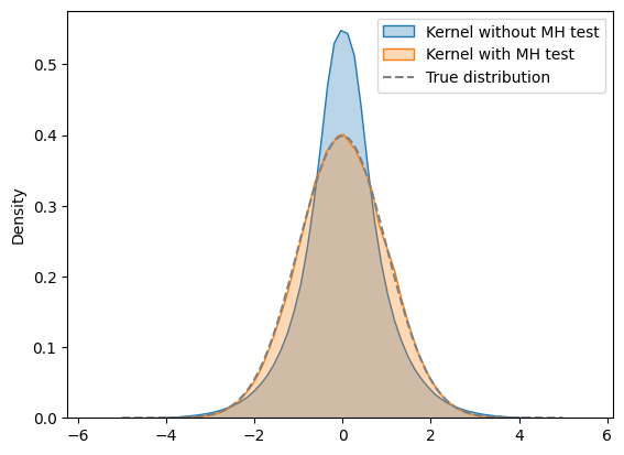
Figure 1: Histogram (polygon style) of samples from MAMS (orange) and MAMS kernel without adjustment (blue). Model: 100-dimensional standard normal (1st dim shown). Ground truth in black. Step size is chosen very large ($\epsilon=20$) to highlight the bias which the MH-test removes.

4 Randomization of the decoherence time

The performance of HMC is known to be very sensitive to the choice of the trajectory length and the problem becomes even more pronounced for ill-conditioned targets, where different directions may require different trajectory lengths for optimal performance. Two approaches to this problem are randomizing the trajectory length (Bou-Rabee & Sanz-Serna, 2017) and replacing the full velocity refreshment with partial refreshment after every step, also known as the Langevin Monte Carlo. We will here pursue both approaches with respect to MAMS.

4.1 Random integration length

We randomize the integration length by taking $n_{k}=\lceil 2h_{k}L/\epsilon\rceil$ integration steps to construct the $k$-th MH proposal. Here $h_{k}$ can either be random draws from the uniform distribution $\mathcal{U}(0,1)$ or the $k$-th element of the Halton’s sequence, as recommended in (Owen, 2017; Hoffman et al., 2021). Other distributions of the trajectory length were also explored in the literature (Sountsov & Hoffman, 2021) but with no gain in performance. The factor of two is inserted to make sure that we do $L/\epsilon$ steps on average.

4.2 Partial refreshment

Partially refreshing the velocity after every step also has the effect of randomizing the time before the velocity coherence is completely lost, and therefore has similar benefits to randomizing the integration length (Jiang, 2023).

However, while the flipping of velocity, needed for the deterministic part of the update to be an involution, is made redundant by a full resampling of velocity, this is not the case for partial refreshment. This results in rejected trajectories backtracking some of the progress that was made in the previously accepted proposals (Riou-Durand & Vogrinc, 2022). Skipping the velocity flip is possible, but it results in a small bias in the stationary distribution (Akhmatskaya et al., 2009) and it is not clear that it has any advantages over full refreshment. Two popular solutions for LMC are to either use a non-reversible MH acceptance probability as in (Hoffman & Sountsov, 2022b) or to add a full momentum refreshment before the MH step as in MALT (Riou-Durand & Vogrinc, 2022). We will here prove that both can be straightforwardly used with Microcanonical dynamics, and then concentrate on the MALT strategy in the remainder of the paper.

We will generate the Langevin dynamics by the “OBABO” scheme (Leimkuhler & Matthews, 2015), where BAB is the deterministic $\varphi_{\epsilon}$ map from Equation 5 and $O$ is the partial velocity refreshment. In LMC, $O_{\epsilon}(\boldsymbol{u})=c_{1}\boldsymbol{u}+c_{2}\boldsymbol{Z}$, where $Z$ is the standard normal distributed variable, $c_{1}=e^{-\epsilon/L_{\mathrm{partial}}}$ and $c_{2}=\sqrt{1-c_{1}^{2}}$. $L_{\mathrm{partial}}$ is parameter that controls the strength of the partial refreshment and is to be comparable with HMC’s trajectory length $L$. With microcanonical dynamics, we typically take a similar expression that additionally normalizes the velocity:

$$O_{\epsilon}(\boldsymbol{u})=\frac{c_{1}\boldsymbol{u}+c_{2}\boldsymbol{Z}/\sqrt{d}}{|c_{1}\boldsymbol{u}+c_{2}\boldsymbol{Z}/\sqrt{d}|}.$$ (12)

Let’s denote by $\Delta(\boldsymbol{z}^{\prime},\boldsymbol{z})$ the energy error accumulated in the deterministic ($\varphi_{\epsilon}$) part of the update. Note that for microcanonical Langevin dynamics, only the deterministic part of the update changes the energy, while in canonical Langevin dynamics, the $O$ update also changes the energy but is not included in $\Delta$.

Theorem 4.1.

The Metropolis-Hastings acceptance probability of the proposal $q(\boldsymbol{z}^{\prime}|\boldsymbol{z})$, corresponding to $\mathcal{T}OBABO$ is $\mathrm{min}(1,\,e^{-\Delta(\boldsymbol{z}^{\prime},\boldsymbol{z})})$.

The MEADS strategy (Hoffman & Sountsov, 2022b) only uses the one-step proposal so Lemma 3.2 shows that it can be generalized to the microcanonical update, simply by using the microcanonical energy instead of canonical energy.

The MALT proposal on the other hand consists of $n$ LMC (or in our case microcanonical LMC) steps and a full refreshment of the velocity, as shown in Algorithm 1.

Algorithm 1 MAMS - Langevin

 Input:

 negative logdensity function $\mathcal{L}:\mathbb{R}^{d}\xrightarrow[]{}\mathbb{R}$

 initial condition $\boldsymbol{x}_{0}\in\mathbb{R}^{d}$

 number of samples $N>0$

 step size $\epsilon>0$

 steps per sample $L/\epsilon\in\mathbb{N}$

 partial refreshment parameter $L_{\mathrm{partial}}$

 Returns: samples $\{\boldsymbol{x}_{n}\}_{n=1}^{N}$ from $p(\boldsymbol{x})$.

 for $I\leftarrow 0$ to $N$ do

  $\boldsymbol{u}\sim\mathcal{U}_{S^{d-1}}$

  $\boldsymbol{z}^{0}\leftarrow(\boldsymbol{x}^{I},\boldsymbol{u})$

  $\delta\leftarrow 0$

  for $i\leftarrow 0$ to $n$ do

   $\boldsymbol{z}\leftarrow O_{\epsilon}(\boldsymbol{z}_{i})$

   $\boldsymbol{z}^{\prime}\leftarrow\Phi_{\epsilon}(\boldsymbol{z})$

   $\boldsymbol{z}^{i+1}\leftarrow O_{\epsilon}(\boldsymbol{z}^{\prime})$

   $\delta\leftarrow\delta+\Delta(\boldsymbol{z}^{\prime},\boldsymbol{z})$

  end for

  draw a random uniform variable $U\sim\mathcal{U}(0,1)$

  if $U<e^{-\delta}$ then

   $\boldsymbol{x}^{I+1}\leftarrow\boldsymbol{z}^{n-1}[0]$

  else

   $\boldsymbol{x}^{I+1}\leftarrow\boldsymbol{z}^{0}[0]$

  end if

 end for

Theorem 4.2.

Sequence $\{\boldsymbol{x}_{i}\}_{i>0}$ defined in Algorithm 1 is a Markov chain whose stationary distribution is $p(\boldsymbol{z})$.

Proofs of both theorems are in Appendix A.

5 Adaptation

MAMS has two hyperparameters, stepsize $\epsilon$ and the trajectory length $L$, where $L/\epsilon$ is the (average) number of steps in a proposal’s trajectory. The Langevin MALT-style version of the algorithm has an additional hyperparameter $L_{\mathrm{partial}}$ that determines the partial refreshment strength during the proposal trajectories, i.e. the amount of Langevin noise. In addition, it is common to use a preconditioning matrix $M$ to linearly transform the configuration space, in order to reduce the condition number of the covariance matrix. The performance of the algorithm crucially depends on these hyperparameters so we here develop an automatic tuning scheme. First, the stepsize is tuned, then the preconditioning matrix, and finally the trajectory length. By default, each stage takes $10\%$ of the total sampling time. $L_{\mathrm{partial}}$ is directly set by the trajectory length, see Section 5.4.

5.1 Stepsize

We will heuristically show that the optimal acceptance rate in MAMS is the same as in HMC, so that a stochastic optimization scheme, such as dual averaging (Nesterov, 2009) can be used to adapt the stepsize (Hoffman et al., 2014).

The optimal acceptance rate argument for MAMS is analogous to the one in (Neal et al., 2011b). We will use two general properties of the deterministic MH proposal:

1. The expected value of the MH ratio under the stationary distribution, $\mathbb{E}_{z\sim p}[e^{-W(z^{\prime},z)}]$, is

   $$\int p(\boldsymbol{z})e^{-W(\boldsymbol{z}^{\prime},\boldsymbol{z})}d\boldsymbol{z}=\int p(\boldsymbol{z})\frac{q(\boldsymbol{z}|\boldsymbol{z}^{\prime})p(\boldsymbol{z}^{\prime})}{q(\boldsymbol{z}^{\prime}|\boldsymbol{z})p(\boldsymbol{z})}d\boldsymbol{z}$$

   $$=\int p(\boldsymbol{z}^{\prime})\big{|}\frac{\partial\varphi}{\partial\boldsymbol{z}}(\boldsymbol{z})\big{|}d\boldsymbol{z}=\int p(\varphi(\boldsymbol{z}))d\varphi(\boldsymbol{z})=1.$$

   This is the Jarzynski equality. In statistical literature it was used by (Neal et al., 2011a; Creutz, 1988) in the special case when $\varphi$ is symplectic.

2. In equilibrium,

   $$P(W>0|\mathrm{accepted})=P(W<0|\mathrm{accepted})=\frac{1}{2}$$

   by the design of the MH test (Neal et al., 2011b). Since $P(\mathrm{accepted}|W<0)=1$, we have that

   $$\frac{1}{2}=P(w<0|\mathrm{accepted})$$

   $$=\frac{P(W<0|\mathrm{accepted})P(W<0)}{P(\mathrm{accepted})}=\frac{P(W<0)}{P(\mathrm{accepted})},$$

   so $P(\mathrm{accepted})=2P(W<0)$.

Let us approximate the stationary distribution over $W$ as $\mathcal{N}(\mu,\sigma^{2})$, as in (Neal, 2011). We then have by the Jarzynski equality:

$$1 =\int p(\boldsymbol{z})e^{-W(\boldsymbol{z}^{\prime},\boldsymbol{z})}d\boldsymbol{z}$$ (13)

$$=\int_{-\infty}^{\infty}\frac{1}{\sqrt{2\pi\sigma^{2}}}e^{-(W-\mu)^{2}/2\sigma^{2}}e^{-W}dW=e^{\frac{\sigma^{2}}{2}-\mu},$$

implying that $\sigma^{2}=2\mu$. By property (2) we then have

$$P(\mathrm{accept})=2\Phi(-\mu/\sqrt{2\mu}),$$ (14)

where $\Phi$ is the Gaussian cumulative density function. Let’s denote by $K_{\mathrm{accepted}}$ the number of accepted proposals that we need for a new effective sample. This corresponds to traveling a distance on the order of the size of the typical set

$$K_{\mathrm{accepted}}N\epsilon\propto\sqrt{d},$$ (15)

since $\sqrt{d}$ is the size of the standard Gaussian’s typical set. The number of effective samples per gradient call is then

$$\mathit{ESS}=\frac{1}{K_{\mathrm{total}}N}=\frac{P(\mathrm{accept})}{K_{\mathrm{accepted}}N}\propto\frac{\epsilon P(\mathrm{accept})}{\sqrt{d}}.$$ (16)

The error of the MCHMC Velocity Verlet integrator for an interval of fixed length is (Robnik & Seljak, 2024)

$$\sigma^{2}/d\propto\epsilon^{4}/d^{2},$$ (17)

implying that $\sigma^{2}=2\mu\propto\epsilon^{4}/d$. Therefore

$$ESS\propto\mu^{1/4}\,\Phi(-\sqrt{\mu/2})\,d^{-1/4},$$ (18)

so we see that the efficiency drops as $d^{-1/4}$. ESS is maximal at $\mu=0.41$, corresponding to $P(\mathrm{accept})=65\%$. From Equation 17 we then see that the optimal stepsize grows as $\epsilon\propto d^{1/4}$ instead of the $d^{1/2}$ that would correspond to the unimpaired efficiency.

Note that this result is different if a higher-order integrator is used. For example, when using a fourth order integrator $\sigma^{2}/d\propto(\epsilon^{2}/d)^{4}$, the optimal setting is $\mu=0.13$ and $P(\mathrm{accept})=80\%$.

Empirically, we find that even for a second-order integrator, targeting a higher acceptance rate, of $90\%$, works well in practice; we use this in our experiments.

5.2 Preconditioning matrix

A simple choice of diagonal preconditioning matrix is obtained by estimating variance along each parameter, which can be done with any sampler. In practice, we use a run of microcanonical dynamics without MH adjustment, since we find it to be the fastest option and asymptotic bias is not a concern here.

5.3 Trajectory length

Microcanonical and canonical dynamics are extremely efficient in exploring the configuration space, while staying on the typical set. Therefore we do not wish to reduce them to a comparatively inefficient diffusion process by adding to much momentum decoherence, i.e. having too low $L$. On the other hand, to maintain efficient exploration, we want to prevent the dynamics to be caught in cycles or quasi cycles.

Heuristically, we should send the dynamics in a new direction at the time scale that the dynamics needs to move to a different part of the configuration space, i.e. produce a new effective sample (Robnik et al., 2024). This suggests two approaches for tuning $L$.

The simpler is to estimate the size of the typical set by computing the average of the eigenvalues of the covariance matrix, which is equal to the mean of the variances in each dimension (Robnik et al., 2024). With a linearly preconditioned target, these variances are 1, and the estimate for the optimal $L$ is $L=\sqrt{d}$. We will use this as an initial value.

A more refined approach is to set $L$ to be on the same scale as the time passed between effective samples:

$$L_{ALBA} \propto\langle\text{time between effective samples}\rangle$$ (19)

$$=\langle\text{time between samples}\rangle\,\tau_{\mathrm{int}}=L\,\tau_{\mathrm{int}},$$

we call this approach Autocorrelation length based adaptation (ALBA). The proportionality constant in the first line is on the order of one and will be determined numerically, based on Gaussian targets. Integrated autocorrelation time $\tau_{\mathrm{int}}$ is the ratio between the total number of (correlated) samples in the chain and the number of effectively uncorrelated samples. It depends on the observable $f(\boldsymbol{x})$ that we are interested in and can be calculated as

$$\tau_{\mathrm{int}}[f]=1+2\sum_{t=1}^{\infty}\rho_{t}[f],$$ (20)

where

$$\rho_{t}[f]=\frac{\mathbb{E}[(f(\boldsymbol{x}(s))-\mathbb{E}[f])(f(\boldsymbol{x}(s+t))-\mathbb{E}[f])]}{\mathrm{Var}[f]}$$ (21)

is the chain autocorrelation function in stationarity. We take $f(x_{i})=x_{i}$ and harmonically average $\tau_{\mathrm{int}}[x_{i}]$ over $i$. We determine the proportionality constant of Equation 19 in a way that $L_{ALBA}$ equals the optimal L, determined by a grid search, for the standard Gaussian. We find a proportionality constant of $0.3$ for MAMS without Langevin noise and $0.23$ with Langevin noise.

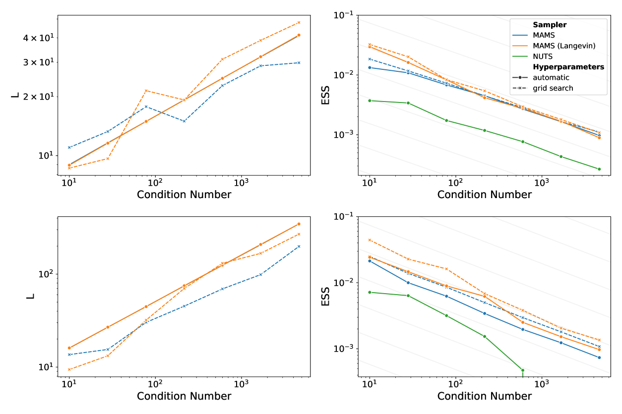
Figure 2: Tuning performance on Gaussians as a function of condition number. Gaussians are 100-dimensional with a log uniform distributed eigenvalues on the top row and outlier distributed eigenvalues on the bottom row. The value of the hyperparameter $L$ obtained from the automatic tuning algorithm is shown on the left (solid line) and compared to the optimal $L$ obtained by a grid search. As can be seen, close to optimal values are obtained. The resulting ESS (on the worst parameter) is shown on the right. Grey lines are $y=x^{-\frac{1}{2}}$

5.4 Langevin noise

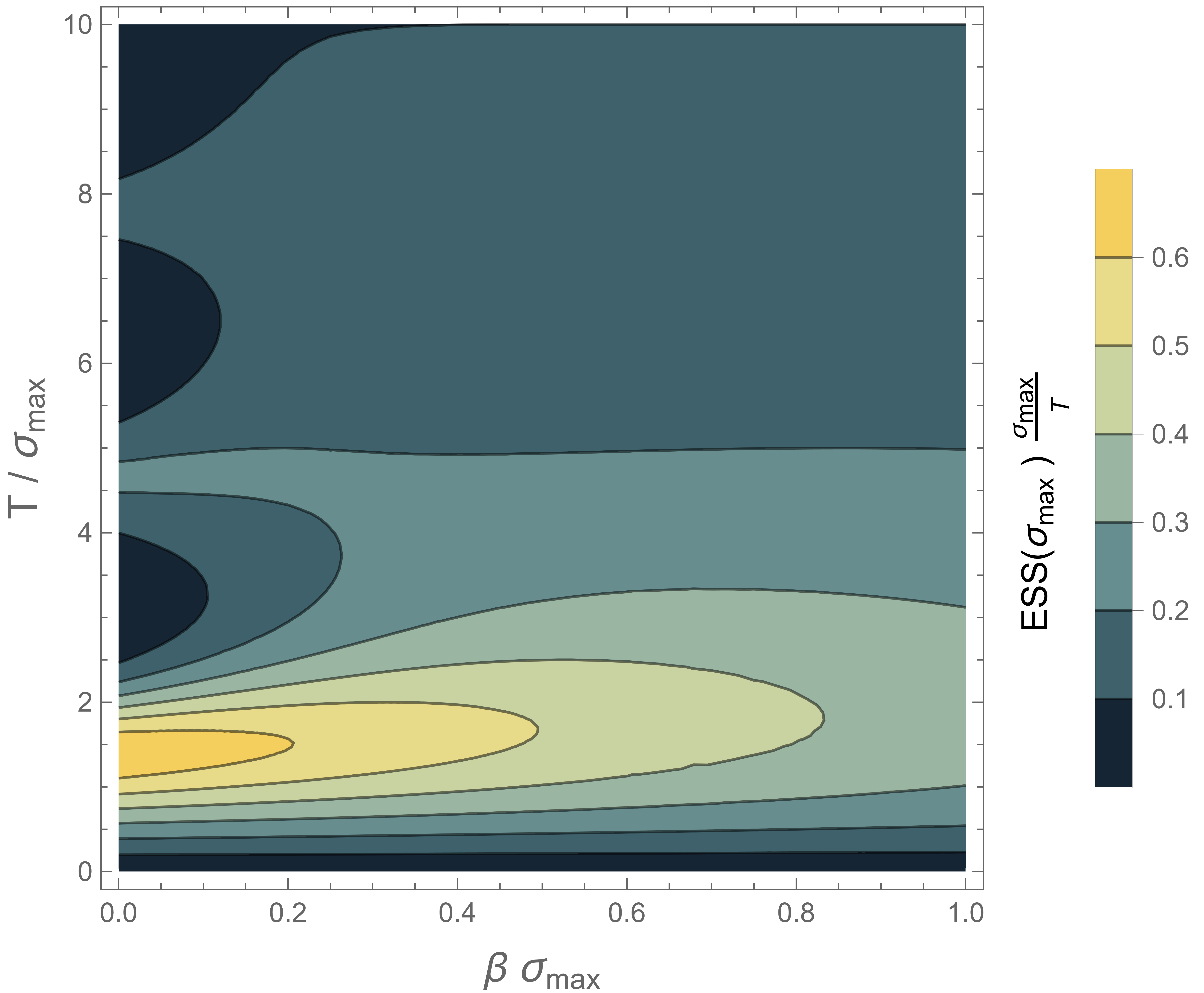
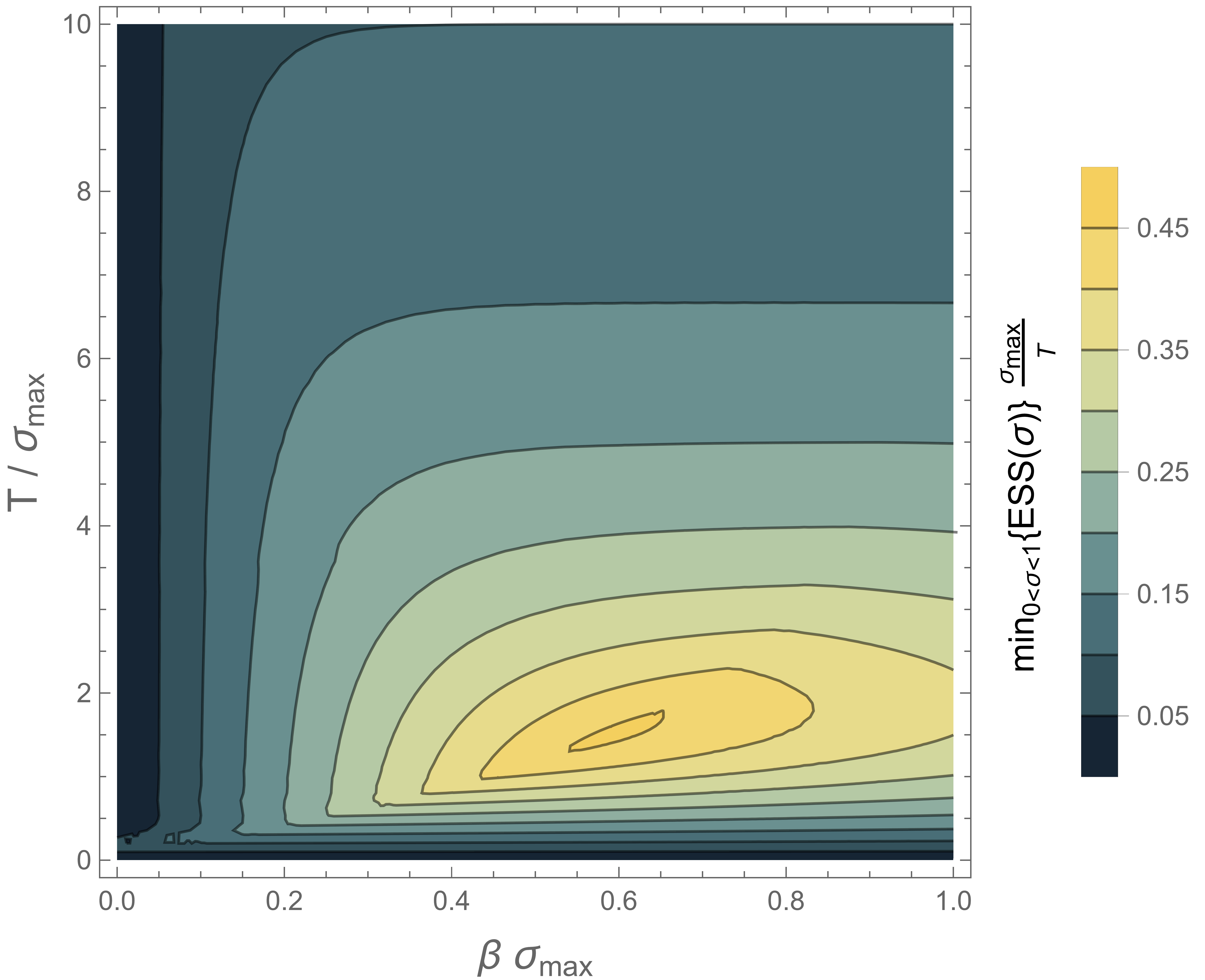
Figure 3: Effective sample size in continuous time for MALT LMC on Gaussian targets. x-axis is the LMC damping parameter, y-axis the trajectory length. $x=0$ is the HMC line, $x=1$ the critically damped LMC. Left panel: isotropic Gaussian $\mathcal{N}(0,\sigma_{\max})$. Note that HMC achieves the optimal performance if properly tuned, the only reason to introduce Langevin noise would be to potentially make the tuning easier. Right panel: extremely ill-conditional Gaussian with all scales $(0,\sigma_{max}]$. ESS along the worst direction is shown. HMC performs poorly as it cannot be tuned to all scales, damping of $\beta\sigma_{max}=0.57$ performs best. Note that these results do not imply MALT having non-zero ESS in the infinite condition number limit: we only study continuous time MALT here.

For MALT, (Riou-Durand & Vogrinc, 2022) derive the ESS of the second moments in the continuous-time limit for the Gaussian targets $\mathcal{N}(0,\sigma)$:

$$ESS(\beta,T)=\frac{1-\rho^{2}}{1+\rho^{2}},$$ (22)

where

$$\rho=e^{-\beta T}\big{(}\cos{\omega T}+\frac{\beta}{\omega}\sin{\omega T}\big{)}\qquad\omega=\sqrt{\frac{1}{\sigma^{2}}-\beta^{2}}.$$ (23)

$T$ is the trajectory length, $\beta$ is the LMC damping parameter ($\gamma=2\beta$ in (Riou-Durand & Vogrinc, 2022)).

Figure 3 shows that the optimal settings for ill conditioned Gaussians are $\beta=0.567$ and $T=1.413$. Therefore the optimal ratio of the decoherence time scales of the partial and full refreshment are

$$\frac{t_{\mathrm{partial}}}{t_{\mathrm{full}}}=\frac{1/\beta}{T}=1.25.$$ (24)

We will use the same setting for Langevin MAMS, so $L_{\mathrm{partial}}/L=1.25$.

6 Experiments

To compare the performance of MAMS to other sampling algorithms such as NUTS, we monitor the convergence of second moments and report the number of gradient calls needed to achieve low error. Following Hoffman & Sountsov 2022a, we define the squared error of the expectation value $f(\boldsymbol{x})$ as

$$b^{2}(f)=\frac{(\mathbb{E}_{\mathrm{sampler}}[f]-\mathbb{E}[f])^{2}}{\mathrm{Var}[f]},$$ (25)

and take the largest second-moment error across parameters:

$$b^{2}_{\mathrm{max}}\equiv\max_{1\leq i\leq d}b^{2}(x_{i}^{2}),$$ (26)

because in our problems of interest, there is typically a parameter of particular interest that has a significantly higher error than the other parameters, for example, a hierarchical parameter in various Bayesian models. We will report the number of gradient calls needed to achieve low error, $b^{2}_{\mathrm{max}}<0.01$. This error can be interpreted as corresponding to 100 effective samples (Hoffman & Sountsov, 2022a).

Figure 2 compares MAMS with NUTS on 100-dimensional Gaussians with varying condition number. Two distributions of covariance matrix eigenvalues are tested: uniform in log and outlier distributed. Outlier distributed means that two eigenvalues are $\kappa$ while the other eigenvalues are $1$. For both samplers, the number of gradients to low error scales with the condition number $\kappa$ as $\kappa^{-\frac{1}{2}}$, but MAMS is faster by a factor of around 4.

	NUTS	MAMS	MAMS (Langevin)
Gaussian	19,652	3,249	3,172
Banana	95,519	14,078	14,818
Rosenbrock	161,359	94,184	103,545
Brownian	29,816	13,528	15,232
GCredit	88,975	55,748	49,979
ItemResp	76,043	45,371	56,902
StochVol	843,768	430,088	510,190
Funnel	$>10^{8}$	2,346,899	1,765,311

Table 1: Number of gradients calls needed to get the squared error on the worst second moment below 0.01. Lower is better; number of gradients is roughly proportional to wall clock time.

Table 1 compares NUTS with MAMS on a set of benchmark problems, mostly adapted from the Inference Gym (Sountsov et al., 2020) problem set; see Appendix C for model details. For both algorithms, we use an initial run to find a preconditioning matrix. For NUTS, the only remaining parameter to tune is step size, which is tuned by dual averaging, targeting $80\%$ acceptance rate. For MAMS, we further tune $L$ using the ALBA scheme of Section 5.3. We take the tuning steps as our burn-in, initializing the chain with the final state returned by the tuning procedure. NUTS is run using the BlackJax (Cabezas et al., 2024) implementation, with the provided window adaptation scheme. Table 1 shows the number of gradient calls in the chain (excluding tuning) used to reach squared error of 0.01. To reduce variance in these results, we run at least 128 chains for each problem, and take the median of the error across chains at each step.

In all cases, MAMS outperforms NUTS, typically by a factor of 2–7. The choice to use Langevin noise over trajectory length randomization has little effect in most cases as is typically also the case for HMC (Jiang, 2023; Riou-Durand et al., 2023). For Neal’s Funnel, we find that we need an acceptance rate of 0.99 for MAMS to converge. We were unable to obtain convergence for NUTS. This problem is a known NUTS failure mode, so it is of note that MAMS converges.

	Grid search	ALBA
Gaussian	3,121	3,249
Banana	15,288	14,078
Rosenbrock	93,782	94,184
Brownian	14,015	13,528
GCredit	52,265	55,748
ItemResp	45,640	45,371
StochVol	431,957	430,088

Table 2: Number of gradient calls to low error (as in Table 1) for MAMS with hyperparameters determined by grid search and by ALBA tuning scheme from Section 5.3. ALBA achieves close to optimal performance.

To assess how successful ALBA tuning scheme from Section 5 is at finding the optimal value of $L$, we perform a grid search over $L$, by first performing a long NUTS run to obtain a covariance matrix and an initial $L$, and then for each new candidate value of $L$, tuning step size by dual averaging with a target acceptance rate of $0.9$. In Table 2 we compare the number of gradients to low error using this optimal $L$ to the run with $L$ determined by ALBA. ALBA performance is very close to optimal on all benchmark problems.

7 Conclusion

Our core contribution is MAMS, an out-of-the-box gradient-based sampler applicable in the same settings as NUTS HMC and intended as an alternative to it. We find substantial performance gains in terms of statistical efficiency and in addition note that MAMS is simple to implement, with very little code change compared to standard HMC and the parallelization benefits compared to NUTS that this implies (Sountsov et al., 2024).

Impact Statement

This paper presents work whose goal is to advance the field of Machine Learning. There are many potential societal consequences of our work, none of which we feel must be specifically highlighted here.

Appendix A Metropolis adjusted Microcanonical Langevin dynamics proofs

Denote by $o(\boldsymbol{z}^{\prime}|\boldsymbol{z})$ the density corresponding to the $O$ update and by $q(\boldsymbol{z}^{\prime}|\boldsymbol{z})$, the density corresponding to the single step proposal $\mathcal{T}OBABO$. We will use a shorthand notation for the time reversal: $\overline{\boldsymbol{z}}=\mathcal{T}(\boldsymbol{z})$ and denote by $\Delta(\boldsymbol{z}^{\prime},\boldsymbol{z})$ the energy error accumulated in the deterministic part of the update.

A.1 Proof of Theorem 4.1

Proof.

For the MH ratio we will need

$$\frac{q(\boldsymbol{z}|\overline{\boldsymbol{z}}^{\prime})}{q(\overline{\boldsymbol{z}^{\prime}}|\boldsymbol{z})} =\frac{\int o(\overline{\boldsymbol{z}}|\boldsymbol{Z}^{\prime})\,\delta(\boldsymbol{Z}^{\prime},\varphi(\boldsymbol{Z}))\,o(\boldsymbol{Z}|\overline{\boldsymbol{z}}^{\prime})d\boldsymbol{Z}d\boldsymbol{Z}^{\prime}}{\int o(\boldsymbol{z}^{\prime}|\boldsymbol{Z}^{\prime})\,\delta(\boldsymbol{Z}^{\prime},\varphi(\boldsymbol{Z}))\,o(\boldsymbol{Z}|\boldsymbol{z})d\boldsymbol{Z}d\boldsymbol{Z}^{\prime}}=\frac{\int o(\overline{\boldsymbol{z}}|\varphi(\boldsymbol{Z}))\,o(\boldsymbol{Z}|\overline{\boldsymbol{z}}^{\prime})d\boldsymbol{Z}}{\int o(\boldsymbol{z}^{\prime}|\varphi(\boldsymbol{Z}))\,o(\boldsymbol{Z}|\boldsymbol{z})d\boldsymbol{Z}},$$ (27)

where we have used the delta function to evaluate the integral over $\boldsymbol{Z}^{\prime}$.

We can further simplify the numerator

$$\int o(\overline{\boldsymbol{z}}|\varphi(\boldsymbol{Z}))\,o(\boldsymbol{Z}|\overline{\boldsymbol{z}}^{\prime})d\boldsymbol{Z} =\int o(\boldsymbol{z}|\,\overline{\varphi(\boldsymbol{Z})}\,)\,o(\overline{\boldsymbol{Z}}|\boldsymbol{z}^{\prime})d\boldsymbol{Z}=\int o(\boldsymbol{z}|\,\overline{\varphi(\overline{\boldsymbol{Z}})}\,)\,o(\boldsymbol{Z}|\boldsymbol{z}^{\prime})d\boldsymbol{Z}$$

$$=\int o(\boldsymbol{z}|\varphi^{-1}(\boldsymbol{Z}))\,o(\boldsymbol{Z}|\boldsymbol{z}^{\prime})d\boldsymbol{Z} =\int o(\boldsymbol{z}|\boldsymbol{Z})\,o(\varphi(\boldsymbol{Z})|\boldsymbol{z}^{\prime})\bigg{|}\frac{\partial\varphi(\boldsymbol{Z})}{\partial\boldsymbol{Z}}\bigg{|}d\boldsymbol{Z}=\int o(\boldsymbol{z}^{\prime}|\varphi(\boldsymbol{Z}))\,o(\boldsymbol{Z}|\boldsymbol{z})\bigg{|}\frac{\partial\varphi(\boldsymbol{Z})}{\partial\boldsymbol{Z}}\bigg{|}d\boldsymbol{Z}.$$

In the first step we have used that $o(\overline{\boldsymbol{x}}|\,\overline{\boldsymbol{y}})=o(\boldsymbol{x}|\,\boldsymbol{y})$ and that time reversal is an involution. In the second step, we have performed a change of variables from $\overline{\boldsymbol{Z}}$ to $\boldsymbol{Z}$ (for which, the Jacobian determinant of the transformation is $1$). In the third step we used that $\overline{\varphi(\overline{\boldsymbol{Z}})}=\varphi^{-1}(\boldsymbol{Z})$. In the fourth step we change variables to $\varphi^{-1}(\boldsymbol{Z})$ instead of $\boldsymbol{Z}$. In the last step we use that $o(\boldsymbol{y}|\,\boldsymbol{x})=o(\boldsymbol{x}|\,\boldsymbol{y})$.

Since $o$ only connects states with the same $\boldsymbol{x}$ there is only one $\boldsymbol{Z}$ which makes the integral nonvanishing and we get

$$\frac{q(\overline{\boldsymbol{z}^{\prime}}|\boldsymbol{z})}{q(\boldsymbol{z}|\overline{\boldsymbol{z}}^{\prime})}=\bigg{|}\frac{\partial\varphi(\boldsymbol{Z})}{\partial\boldsymbol{Z}}\bigg{|},$$

as if there were no O updates. The O updates also preserve the target density, so we see that the acceptance probability is only concerned with the BAB part of the update. In this case, the desired acceptance probability was already derived in Lemma 3.2. ∎

A.2 Proof of Theorem 4.2

Proof.

Following a similar structure of the proof as in (Riou-Durand & Vogrinc, 2022) we will work on the space of trajectories $\boldsymbol{z}_{0:L}=(\boldsymbol{z}_{0},\ldots,\boldsymbol{z}_{L})\in\mathcal{M}^{L+1}$. We will define a kernel $\mathcal{Q}$ on the space of trajectories, with $q$ as a marginal-$\boldsymbol{x}_{0}$ kernel. We will prove that $\mathcal{Q}$ is reversible with respect to the extended density

$$\mathcal{P}(\boldsymbol{z}_{0:L})=\prod_{i=1}^{L}q(\boldsymbol{z}_{i}|\boldsymbol{z}_{i-1})p(\boldsymbol{z}_{0}),$$

and use it to show that $q$ is reversible with respect to the marginal $p(\boldsymbol{x}_{0})$.

We define the Gibbs update, corresponding to the conditional distribution $\mathcal{P}(\cdot|\boldsymbol{x}_{0})$:

$$\mathcal{G}(\boldsymbol{z}^{\prime}_{0:L}|\boldsymbol{z}_{0:L})=\delta(\boldsymbol{x}^{\prime}_{0}-\boldsymbol{x}_{0})U_{S^{d-1}}(\boldsymbol{u}^{\prime}_{0})\prod_{i=1}^{L}q(\boldsymbol{z}^{\prime}_{i}|\boldsymbol{z}^{\prime}_{i-1}).$$

The Gibbs kernel $\mathcal{G}$ is reversible with respect to $\mathcal{P}$ by construction. Built upon a deterministic proposal of the backward trajectory

$$\overline{\boldsymbol{z}}_{0:L}=(\overline{\boldsymbol{z}}_{L},\overline{\boldsymbol{z}}_{L-1},\ldots,\overline{\boldsymbol{z}}_{0}),$$ (28)

we introduce a Metropolis update:

$$M(\boldsymbol{z}^{\prime}_{0:L}|\boldsymbol{z}_{0:L})=P_{MH}\,\delta(\boldsymbol{z}^{\prime}_{0:L}-\overline{\boldsymbol{z}}_{0:L})+(1-P_{MH})\delta(\boldsymbol{z}^{\prime}_{0:L}-\boldsymbol{z}_{0:L}),$$

where $P_{MH}(\boldsymbol{z}_{0:L})=\mathrm{min}(1,e^{-\Delta(\boldsymbol{z}_{0:L})})$. For $\eta>0$, the distribution $\mathcal{P}$ admits a density with respect to Lebesgue’s measure. Therefore

$$e^{-\Delta(\boldsymbol{z}_{0:L})}=\frac{\mathcal{P}(\overline{\boldsymbol{z}}_{0:L})}{\mathcal{P}(\boldsymbol{z}_{0:L})}\bigg{|}\frac{\partial\overline{\boldsymbol{z}}_{0:L}}{\partial\boldsymbol{z}_{0:L}}\bigg{|}$$ (29)

ensures that the Metropolis kernel $M$ is reversible with respect to $\mathcal{P}$.

Before proceeding with the proof, we express Equation 29 in a simple, easy-to-compute form. The Jacobian is $\frac{\partial\overline{\boldsymbol{z}}_{0:L}}{\partial\boldsymbol{z}_{0:L}}=\sigma\otimes\frac{\partial\overline{\boldsymbol{z}}}{\partial\boldsymbol{z}}$, where $\sigma$ is the matrix of the permutation $\sigma(i)=L-i$ and $\frac{\partial\overline{\boldsymbol{z}}}{\partial\boldsymbol{z}}=I_{d\times d}\oplus-I_{d-1\times d-1}$. Both of these matrices have determinant $\pm 1$, so the determinant of their Kronecker product is also $\pm 1$ and its absolute value is 1.

We get

$$e^{-\Delta(\boldsymbol{z}_{0:L})} =\frac{\mathcal{P}(\overline{\boldsymbol{z}}_{0:L})}{\mathcal{P}(\boldsymbol{z}_{0:L})}=\frac{p(\overline{\boldsymbol{z}}_{L})\prod_{i=1}^{L}q(\overline{\boldsymbol{z}}_{i-1}|\overline{\boldsymbol{z}}_{i})}{p(\boldsymbol{z}_{0})\prod_{i=1}^{L}q(\boldsymbol{z}_{i}|\boldsymbol{z}_{i-1})}=\frac{\prod_{i=1}^{L}p(\overline{\boldsymbol{z}}_{i})\prod_{i=1}^{L}q(\overline{\boldsymbol{z}}_{i-1}|\overline{\boldsymbol{z}}_{i})}{\prod_{i=1}^{L}p(\boldsymbol{z}_{i-1})\prod_{i=1}^{L}q(\boldsymbol{z}_{i}|\boldsymbol{z}_{i-1})}=\prod_{i=1}^{L}\frac{q(\overline{\boldsymbol{z}}_{i-1}|\overline{\boldsymbol{z}}_{i})p(\overline{\boldsymbol{z}}_{i})}{q(\boldsymbol{z}_{i}|\boldsymbol{z}_{i-1})p(\boldsymbol{z}_{i-1})}$$ (30)

$$=e^{-\sum_{i=1}^{L}\Delta(\boldsymbol{z}_{i},\boldsymbol{z}_{i-1})},$$

where $\Delta(\boldsymbol{z}_{i},\boldsymbol{z}_{i-1})$ is the energy error in step $i$, by Theorem 4.1.

We are now in a position to define the trajectory-space kernel:

$$\mathcal{Q}=\mathcal{G}M\mathcal{G}.$$ (31)

The palindromic structure of $\mathcal{Q}$ ensures reversibility with respect to $\mathcal{P}$. Since the transition $\mathcal{G}(\cdot|\boldsymbol{z}_{0:L})=\mathcal{G}(\cdot|\boldsymbol{x}_{0})$ only depends on the starting position $\boldsymbol{x}_{0}\in\mathbb{R}^{d}$ and $p(\boldsymbol{x})$ is the marginal of $\mathcal{P}$, we obtain that $q(\boldsymbol{x}^{\prime}_{0}|\boldsymbol{x}_{0})=\int\mathcal{Q}(\boldsymbol{z}^{\prime}_{0:L}|\boldsymbol{z}_{0:L})d\boldsymbol{u}_{0}\prod_{i=1}^{L}d\boldsymbol{z}_{i}$ defines marginally a Markov kernel on $\mathbb{R}^{d}$, reversible with respect to $p$. In particular, the distribution of $\{\boldsymbol{x}_{i}\}_{i\geq 0}$ in Algorithm 1 coincides with the distribution of a Markov chain generated by $q$. ∎

Appendix B Microcanonical dynamics

In this appendix, we establish a relationship between the microcanonical dynamics of Equation 3 and a Hamiltonian system with energy $E$ from which it can be derived by a time-rescaling operation. As well as motivating the dynamics of Equation 3, this allows us to show that $W$ in Lemma 3.2 for the dynamics of Equation 3 corresponds to the change in energy $E$ of the Hamiltonian system. We also provide a complete derivation of the form of $W$ for microcanonical dynamics. Familiarity with the basics of Hamiltonian mechanics is assumed throughout.

B.1 Sundman transformation

We begin by introducing a transformation to a Hamiltonian system known as a Sundman transform (Leimkuhler & Reich, 2004)

$$S(F)(\boldsymbol{z}(t))=w(\boldsymbol{z}(t))F(\boldsymbol{z}(t)),$$

where $w$ is any function $\mathbb{R}^{2d}\to\mathbb{R}$. Intuitively, this is a $\boldsymbol{z}$-dependent time rescaling of the dynamics. Therefore it is not surprising that:

Lemma B.1.

The integral curves of $S(F)$ are the same as of $F$ (Skeel, 2009)

Proof.

To see this, first use $\boldsymbol{z}_{G}$ to refer to the dynamics from a field $G$, and posit that $\boldsymbol{z}_{S(F)}(s)=\boldsymbol{z}_{F}(t(s))$, where $\frac{dt(s)}{ds}=w(\boldsymbol{z}(s))$. Then we see that

$$\frac{d\boldsymbol{z}_{S(F)}(s)}{dt}=\frac{d\boldsymbol{z}_{F}(t(s))}{ds}=\frac{d\boldsymbol{z}_{F}(t)}{dt}\frac{dt}{ds}=F(\boldsymbol{z}_{F}(s))w(\boldsymbol{z}_{F}(s)),$$

which shows that, indeed, $\boldsymbol{z}_{S(F)}=\boldsymbol{z}_{F}\circ s$, where $s$ is a function $\mathbb{R}\to\mathbb{R}$, which amounts to what we set out to show.

∎

However, note that the stationary distribution is not necessarily preserved, on account of the phase space dependence of the time-rescaling, which means that in a volume of phase space, different particles will move at different velocities.

B.2 Obtaining the dynamics of Equation 3

Consider the Hamiltonian system given by $H=T+V$, with $T(\boldsymbol{\Pi})=(d-1)\log|\boldsymbol{\Pi}|$ and $V(\boldsymbol{x})=\mathcal{L}(\boldsymbol{x})$. Then the dynamics derived from Hamilton’s equations of motion are:

$$\frac{d}{dt}\begin{bmatrix}\boldsymbol{x}\\ \boldsymbol{\Pi}\end{bmatrix}=\begin{bmatrix}\frac{\partial H}{\partial\boldsymbol{\Pi}}\\ -\frac{\partial H}{\partial\boldsymbol{x}}\end{bmatrix}=\begin{bmatrix}(d-1)\frac{\boldsymbol{\Pi}}{|\boldsymbol{\Pi}|^{2}}\\ -\nabla_{\boldsymbol{x}}\mathcal{L}(\boldsymbol{x})\end{bmatrix}:=F(\boldsymbol{z}).$$ (32)

Any Hamiltonian dynamics has $p(\boldsymbol{z})\propto\delta(H-C)$ as a stationary distribution, which can be sampled from by integrating the equations if ergodicity holds. As observed in (Ver Steeg & Galstyan, 2021) and (Robnik et al., 2024), the closely related Hamiltonian $d\log|\boldsymbol{\Pi}|+\mathcal{L}(\boldsymbol{x})$ has the property that the marginal of this stationary distribution is the desired target, namely $p(\boldsymbol{x})\propto e^{-\mathcal{L}(\boldsymbol{x})}$. However, numerical integration of these equations is unstable due to the $\frac{1}{|\boldsymbol{\Pi}|^{2}}$ factor, and moreover, MH adjustment is not possible since numerical integration induces error in $H$, which would result in proposals always being rejected, due to the delta function.

Both problems can be addressed with a Sundman transform and a subsequent change of variables. To that end, we choose $w(\boldsymbol{z})=|\boldsymbol{\Pi}|/(d-1)$ (which corresponds, up to a factor, to the weight $r$ in (Ver Steeg & Galstyan, 2021), and to $w$ in (Robnik et al., 2024)), we obtain:

$$\frac{d}{dt}\begin{bmatrix}\boldsymbol{x}\\ \boldsymbol{\Pi}\end{bmatrix}=\begin{bmatrix}\boldsymbol{\Pi}/|\boldsymbol{\Pi}|\\ -\nabla\mathcal{L}(\boldsymbol{x})|\boldsymbol{\Pi}|/(d-1)\end{bmatrix}.$$ (33)

Changing variables to $\boldsymbol{u}=\boldsymbol{\Pi}/|\boldsymbol{\Pi}|$, we obtain precisely the microcanonical dynamics of Equation 3:

$$\frac{d}{dt}\begin{bmatrix}\boldsymbol{x}\\ \boldsymbol{u}\end{bmatrix}=\begin{bmatrix}\boldsymbol{u}\\ -(I-\boldsymbol{u}\boldsymbol{u}^{T})\nabla\mathcal{L}(\boldsymbol{x})/(d-1)\end{bmatrix}:=\begin{bmatrix}B_{\boldsymbol{x}}\\ B_{\boldsymbol{u}}\end{bmatrix},$$

where we have used that the Jacobian $\frac{d\boldsymbol{u}}{d\boldsymbol{\Pi}}=\frac{1}{|\boldsymbol{\Pi}|}(I-\frac{\boldsymbol{\Pi}\boldsymbol{\Pi}^{T}}{|\boldsymbol{\Pi}|^{2}})$. Note that $B_{\boldsymbol{x}}=S(F)_{\boldsymbol{x}}$, since this final change of variable only targets $\boldsymbol{\Pi}$.

B.3 Discrete updates

For completeness, we here state the position and velocity updates of the canonical and microcanonical dynamics, which are obtained by solving dynamics at fixed velocity for the position update and at fixed position for the velocity update. For canonical dynamics, this amounts to solving

$$\frac{d}{d\epsilon}A_{\epsilon}=\boldsymbol{u}(t)\qquad\frac{d}{d\epsilon}B_{\epsilon}=-\nabla\mathcal{L}(\boldsymbol{x}(t)),$$ (34)

with initial condition $A_{0}=\boldsymbol{x}(t)$ and $B_{0}=\boldsymbol{u}(t)$. These solution is trivial:

$$A_{\epsilon}=\boldsymbol{x}(t)+\epsilon\boldsymbol{u}(t)\qquad B_{\epsilon}=\boldsymbol{u}(t)-\epsilon\nabla\mathcal{L}(\boldsymbol{x}(t)).$$ (35)

For microcanonical dynamics, one needs to solve

$$\frac{d}{d\epsilon}A_{\epsilon}=\boldsymbol{u}(t)\qquad\frac{d}{d\epsilon}B_{\epsilon}=-(1-\boldsymbol{u}(t)\boldsymbol{u}(t)^{T})\nabla\mathcal{L}(\boldsymbol{x}(t))/(d-1),$$ (36)

with initial condition $A_{0}=\boldsymbol{x}(t)$ and $B_{0}=\boldsymbol{u}(t)$. The velocity equation is a vector version of the Riccati equation (Ver Steeg & Galstyan, 2021). Let’s denote $\boldsymbol{g}=-\nabla\mathcal{L}(\boldsymbol{x}(t))/(d-1)$ and replace the variable $B_{\epsilon}$ by $\boldsymbol{y}_{\epsilon}$, such that

$$B_{\epsilon}=\frac{\frac{d}{d\epsilon}\boldsymbol{y}_{\epsilon}}{\boldsymbol{g}\cdot\boldsymbol{y}_{\epsilon}}.$$ (37)

This is convenient, because the equation for $B_{\epsilon}$ is a nonlinear first-order differential equation, but the equation for $\boldsymbol{y}_{\epsilon}$ is a linear second-order differential equation

$$\frac{d^{2}}{d\epsilon^{2}}\boldsymbol{y}_{\epsilon}=(\boldsymbol{g}\boldsymbol{g}^{T})\boldsymbol{y}_{\epsilon},$$ (38)

which is easy to solve and yields the updates

$$A_{\epsilon}=\boldsymbol{x}(t)+\epsilon\boldsymbol{u}(t)\qquad B_{\epsilon}=\frac{\boldsymbol{u}(t)+(\sinh{\delta}+\boldsymbol{e}\cdot\boldsymbol{u}(t)(\cosh\delta-1))\boldsymbol{e}}{\cosh{\delta}+\boldsymbol{e}\cdot\boldsymbol{u}(t)\sinh{\delta}},$$ (39)

where $\delta=\epsilon|\nabla\mathcal{L}(\boldsymbol{x}(t))|/(d-1)$ and $\boldsymbol{e}=-\nabla\mathcal{L}(\boldsymbol{x})/|\nabla\mathcal{L}(\boldsymbol{x})|$.

B.4 Obtaining the stationary distribution of Equation 3

We can derive the stationary distribution of Equation 3 following the approach of (Tuckerman, 2023). There, it is shown that for a flow $F$, if there is a $g$ such that $\frac{d}{dt}\log g=-\nabla\cdot F$, and $\Lambda$ is the conserved quantity under the dynamics, then $p(\boldsymbol{z})\propto g(\boldsymbol{z})f(\Lambda(\boldsymbol{z}))$, where $f$ is any function.

We note that $\nabla\cdot F=\boldsymbol{u}\cdot\nabla\mathcal{L}(x)=\frac{d}{dt}\mathcal{L}(\boldsymbol{x})$, using Section B.7 in the first step. Therefore $\log g=-\mathcal{L}(\boldsymbol{x})$. Further, $|\boldsymbol{u}|$ is preserved by the dynamics if we initialize with $|\boldsymbol{u}_{0}|=1$, as can easily be seen: $\frac{d}{dt}(\boldsymbol{u}\cdot\boldsymbol{u})=2\boldsymbol{u}\cdot\dot{\boldsymbol{u}}=2\boldsymbol{u}\cdot(I-\boldsymbol{u}\boldsymbol{u}^{T})(-\nabla\mathcal{L}(\boldsymbol{x})/(d-1))=2(1-\boldsymbol{u}\cdot\boldsymbol{u})(\boldsymbol{u}\cdot-\nabla\mathcal{L}/(d-1))=0$. Thus a stationary distribution is:

$$p(\boldsymbol{x},\boldsymbol{u})\propto e^{-{\mathcal{L}(\boldsymbol{x})}}\delta(|u|-1).$$ (40)

Importantly, because even the discretized dynamics are norm preserving, the condition $\delta(|\boldsymbol{u}|-1)$ is always satisfied, so that $\frac{p(\boldsymbol{z}^{\prime})}{p(\boldsymbol{z})}$ is always well defined. This makes it possible to perform MH adjustment, in contrast to the original Hamiltonian dynamics as discussed in Section B.2.

B.5 $W$ as energy change

In the non-equilibrium physics literature, $W$ (termed the dissipation function) is interpreted as work done on the system and the second term in Lemma 3.1 is the dissipated heat (Evans & Searles, 1994, 2002; Sevick et al., 2008). $W$ plays a central role in fluctuation theorems, for example, Crook’s relation (Crooks, 1999) states that the transitions $\boldsymbol{z}\xrightarrow[]{}\boldsymbol{z}^{\prime}$ are more probable than $\boldsymbol{z}^{\prime}\xrightarrow[]{}\boldsymbol{z}$ by a factor $e^{W(\boldsymbol{z}^{\prime},\boldsymbol{z})}$. In statistics, this fact is used by the MH test to obtain reversibility, or detailed balance, a sufficient condition for convergence to the target distribution.

Here we will justify why it can also be interpreted as an energy change in microcanonical dynamics.

Lemma B.2.

$W$, calculated for the microcanonical dynamics over a time interval $[0,T]$ is equal to $\Delta E$ of the Hamiltonian $(d-1)\log|\boldsymbol{\Pi}|+\mathcal{L}(\boldsymbol{x})$ for an interval $[s(0),s(T)]$, where $s$ is the time rescaling arising from the Sundman transformation $w(\boldsymbol{z})=|\boldsymbol{\Pi}_{F}|/(d-1)$.

Proof.

Recall that for a flow field $F$:

$$W(\boldsymbol{z}_{F}(T),\boldsymbol{z}_{F}(0))=-\log\frac{p(\boldsymbol{z}_{F}(T))}{p(\boldsymbol{z}_{F}(0))}-\int_{0}^{T}\nabla\cdot F(\boldsymbol{z}_{F}(s))ds$$ (41)

Given the form of the stationary distribution induced by $B$, derived in Section B.4, we see that the first term of the work, $\log\frac{P(\boldsymbol{z}_{B}(0))}{P(\boldsymbol{z}_{B}(T))}=\mathcal{L}(\boldsymbol{x}_{B}(T))-\mathcal{L}(\boldsymbol{x}_{B}(0))=\mathcal{L}(\boldsymbol{x}_{S(F)}(T))-\mathcal{L}(\boldsymbol{x}_{S(F)}(0))=\mathcal{L}(\boldsymbol{x}_{F}(s(T)))-\mathcal{L}(\boldsymbol{x}_{F}(s(0)))$ which is equal to $\Delta V$ for an interval of time $[s(0),s(T)]$.

As for the second term, observe that

$$\frac{dK(\boldsymbol{\Pi}(t(s)))}{ds}=\frac{\partial H}{\partial\boldsymbol{\Pi}}\cdot\frac{d\boldsymbol{\Pi}}{dt}\frac{dt}{ds}=\frac{d\boldsymbol{x}}{dt}\frac{dt}{ds}\cdot\frac{d\boldsymbol{\Pi}}{dt}=\boldsymbol{u}\cdot(-\nabla\mathcal{L}(\boldsymbol{x}))=-\nabla\cdot B,$$

which is precisely the integrand of the second term.

∎

This shows that $W=\Delta K+\Delta V=\Delta E$, where $\Delta E$ is the energy change of the original Hamiltonian, over the rescaled time interval $[s(0),s(T)]$ . As we know, $\Delta E=0$ for the exact Hamiltonian flow, and indeed $W=0$ for the exact dynamics of Equation 3, which is to say that for the exact dynamics, no MH correction would be needed for an asymptotically unbiased sampler.

However, our practical interest is in the discretized dynamics arising from a Velocity Verlet numerical integrator. In this case, we wish to calculate $W$ for $B_{\boldsymbol{u}}$ and $B_{\boldsymbol{x}}$ separately, and consider the sum, noting that $W$ is an additive quantity with respect to the concatenation of two dynamics. Considering $W$ with respect to only $B_{\boldsymbol{x}}$, we see that the first term of $W$ remains $\Delta V$, since the stationary distribution gives uniform weight to all values of $\boldsymbol{u}$ of unit norm, and the dynamics are norm preserving. The second term vanishes, because $\nabla_{\boldsymbol{x}}B_{\boldsymbol{x}}=\nabla_{\boldsymbol{x}}\boldsymbol{u}=0$. As for $B_{\boldsymbol{u}}$, since the norm preserving change in $\boldsymbol{u}$ leaves the density unchanged, the first term of $W$ vanishes. Meanwhile, the second term is $\Delta K$, from the above derivation, since $\nabla\cdot B=\nabla_{\boldsymbol{x}}\cdot B_{\boldsymbol{x}}+\nabla_{\boldsymbol{u}}\cdot B_{\boldsymbol{u}}=\nabla_{\boldsymbol{u}}\cdot B_{\boldsymbol{u}}$. Thus, the full $W$ is equal to $\Delta V+\Delta K=\Delta E$, as desired. For HMC, it is easily seen that $W$ for $F_{\boldsymbol{x}}$ is $\Delta V$, and for $F_{\boldsymbol{u}}$ is $\Delta T$. Putting this together, we maintain the result of Lemma B.2, but now in a setting where $W$ is not $0$ so that MH adjustment is of use.

B.6 Direct calculation of velocity update $W$

We here provide a self-contained derivation of the MH ratio for the velocity update from Equation 39. The MH ratio is a scalar with respect to state space transformations, i.e. it is the same in all coordinate systems. We can therefore select convenient coordinates for its computation. We will choose spherical coordinates in which $\boldsymbol{e}$ is the north pole and

$$\boldsymbol{u}=\cos\vartheta\boldsymbol{e}+\sin\vartheta\boldsymbol{f},$$ (42)

for some unit vector $\boldsymbol{f}$, orthogonal to $\boldsymbol{e}$. $\vartheta$ is then a coordinate on the $S^{d-1}$ manifold. The momentum updating map from Equation 39,

$$\boldsymbol{u}^{\prime}=\frac{1}{\cosh\delta+\cos\vartheta\sinh\delta}\boldsymbol{u}+\frac{\sinh\delta+\cos\vartheta(\cosh\delta-1)}{\cosh\delta+\cos\vartheta\sinh\delta}\boldsymbol{e}=\frac{\sinh\delta+\cos\vartheta\cosh\delta}{\cosh\delta+\cos\vartheta\sinh\delta}\boldsymbol{e}+\frac{\sin\vartheta}{\cosh\delta+\cos\vartheta\sinh\delta}\boldsymbol{f},$$ (43)

can be expressed in terms of the $\vartheta$ variable:

$$\cos\vartheta^{\prime}=\frac{\sinh\delta+\cos\vartheta\cosh\delta}{\cosh\delta+\cos\vartheta\sinh\delta}\qquad\sin\vartheta^{\prime}=\frac{\sin\vartheta}{\cosh\delta+\cos\vartheta\sinh\delta}.$$ (44)

The Jacobian of the $\vartheta\mapsto\vartheta^{\prime}$ transformation is

$$\bigg{|}\frac{d\vartheta^{\prime}}{d\vartheta}\bigg{|}=\bigg{|}\frac{d\vartheta^{\prime}}{d\cos\vartheta^{\prime}}\frac{d\cos\vartheta^{\prime}}{d\vartheta}\bigg{|}=\frac{1}{|\cosh\delta+\cos\vartheta\sinh\delta|}$$ (45)

and the density ratio is

$$\frac{p(\vartheta^{\prime})}{p(\vartheta)}=\sqrt{\frac{g(\vartheta^{\prime})}{g(\vartheta)}}=\bigg{(}\frac{\sin\vartheta^{\prime}}{\sin\vartheta}\bigg{)}^{d-2}=\frac{1}{(\cosh\delta+\cos\vartheta\sinh\delta)^{d-2}},$$ (46)

where $g$ is the metric determinant on a $S^{d-1}$ sphere. Combining the two together yields

$$W=(d-1)\log\big{(}\cosh{\delta}+\cos\vartheta\sinh{\delta}\big{)},$$ (47)

which is the kinetic energy from Equation (8).

B.7 Direct calculation of the velocity update divergence

For completeness, we here derive the divergence of the microcanonical velocity update flow field $F$. We will use the divergence theorem, which states that the integral of the divergence of a vector field over some volume $\Omega$ equals the flux of this vector field over the boundary of $\Omega$. Here, flux is $F\cdot n$ where $n$ is the unit vector, normal to the boundary.

We will use the coordinate system defined in Equation 42 and pick as the volume $\Omega$ a thin spherical shell, centered around the north pole $\boldsymbol{e}$ and spanning the $\vartheta$ range $[\vartheta,\vartheta+\Delta\vartheta]$. The boundary of $\Omega$ are two spheres in $d-2$ dimensions with radia $\sin\vartheta$ and $\sin(\vartheta+\Delta\vartheta)$. Note that $F$ is normal to this boundary and flux is a constant on each shell. It is outflowing on the boundary which is closer to the north pole and inflowing on the other boundary.

Note that for $\Delta\vartheta\xrightarrow[]{}0$, we have that $\nabla\cdot F$ is a constant on $\Omega$. The divergence theorem in this limit therefore implies

$$(\nabla\cdot F)\,V(S^{d-2})(\sin\vartheta)^{d-2}=-\frac{d}{d\vartheta}\big{(}|F|V(S^{d-2})(\sin\vartheta)^{d-2}\big{)},$$ (48)

where $V(S^{d-2})$ is the volume of the unit sphere in d-2 dimensions and we have used that the volume of a $n$-dimensional sphere with radius $r$ is $V(S^{n})r^{n}$. By rearranging we get:

$$\nabla\cdot F=-\frac{\frac{d}{d\vartheta}\big{(}|F|(\sin\vartheta)^{d-2}\big{)}}{(\sin\vartheta)^{d-2}}.$$ (49)

We have

$$F=\frac{|\nabla\mathcal{L}(\boldsymbol{x})|}{d-1}(1-\boldsymbol{u}\boldsymbol{u}^{T})\boldsymbol{e},$$ (50)

so

$$|F|=\frac{|\nabla\mathcal{L}(\boldsymbol{x})|}{d-1}\sqrt{\boldsymbol{e}(1-\boldsymbol{u}\boldsymbol{u}^{T})\boldsymbol{e}}=\frac{|\nabla\mathcal{L}(\boldsymbol{x})|}{d-1}\sqrt{1-(\boldsymbol{e}\cdot\boldsymbol{u})^{2}}=\frac{|\nabla\mathcal{L}(\boldsymbol{x})|}{d-1}\sin\vartheta.$$ (51)

Inserting $|F|$ in Equation 49 yields

$$\nabla\cdot F=-\frac{|\nabla\mathcal{L}(\boldsymbol{x})|}{d-1}\frac{(d-1)(\sin\vartheta)^{d-2}\cos\vartheta}{(\sin\vartheta)^{d-2}}=-|\nabla\mathcal{L}|\boldsymbol{e}\cdot\boldsymbol{u}.$$ (52)

Appendix C Benchmark inference models

We here give some details of the inference models used in Section 6. For models addapted from the Inference gym (Sountsov et al., 2020) we give model’s inference gym name in the parenthesis.

• Gaussian is 100-dimensional with condition number 100 and eigenvalues uniformly spaced in log.

• Banana (Banana) is a two-dimensional, banana-shaped target.

• Rosenbrock is a banana-shaped target in 36 dimensions. It is 18 copies of the Rosenbrock functions with Q = 0.1, see (Grumitt et al., 2022).

• Brownian Motion (BrownianMotionUnknownScalesMissingMiddleObservations) is a 32-dimensional hierarchical problem, where Brownian motion with unknown innovation noise is fitted to the noisy and partially missing data.

• Sparse logistic regression (GermanCreditNumericSparseLogisticRegression) is a 51-dimensional Bayesian hierarchical model, where logistic regression is used to model the approval of the credit based on the information about the applicant.

• Item Response theory (SyntheticItemResponseTheory) is a 501-dimensional hierarchical problem where students’ ability is inferred, given the test results.

• Stochastic Volatility is a 2429-dimensional hierarchical non-Gaussian random walk fit to the S&P500 returns data, adapted from numpyro (Phan et al., 2019)

• Neal’s funnel (Neal, 2011) is a funnel shaped target with a hierarchical parameter $z_{1}\sim\mathcal{N}(0,3)$ that controls the variance of the other parameters $z_{i}\sim\mathcal{N}(0,e^{z_{1}/2})$ for $i=2,3,\ldots d$. We take $d=20$.

Ground truth expectation values ${\mathbb{E}[x^{2}]}$ and ${\mathrm{Var}[x^{2}]}={\mathbb{E}[(x^{2}-{\mathbb{E}[x^{2}]})^{2}]}$ are computed analytically for the Ill Conditioned Gaussian, by generating exact samples for Banana, Rosenbrock and Neal’s funnel and by very long NUTS runs for the other targets.

References

- Akhmatskaya et al. (2009) Akhmatskaya, E., Bou-Rabee, N., and Reich, S. A comparison of generalized hybrid monte carlo methods with and without momentum flip. Journal of Computational Physics, 228(6):2256–2265, 2009.
- Betancourt (2017) Betancourt, M. A conceptual introduction to hamiltonian monte carlo. arXiv preprint arXiv:1701.02434, 2017.
- Bou-Rabee & Sanz-Serna (2017) Bou-Rabee, N. and Sanz-Serna, J. M. Randomized hamiltonian monte carlo. 2017.
- Cabezas et al. (2024) Cabezas, A., Corenflos, A., Lao, J., Louf, R., Carnec, A., Chaudhari, K., Cohn-Gordon, R., Coullon, J., Deng, W., Duffield, S., et al. Blackjax: Composable bayesian inference in jax. arXiv preprint arXiv:2402.10797, 2024.
- Carpenter et al. (2017) Carpenter, B., Gelman, A., Hoffman, M. D., Lee, D., Goodrich, B., Betancourt, M., Brubaker, M. A., Guo, J., Li, P., and Riddell, A. Stan: A probabilistic programming language. Journal of statistical software, 76, 2017.
- Creutz (1988) Creutz, M. Global monte carlo algorithms for many-fermion systems. Physical Review D, 38(4):1228, 1988.
- Crooks (1999) Crooks, G. E. Entropy production fluctuation theorem and the nonequilibrium work relation for free energy differences. Physical Review E, 60(3):2721–2726, September 1999. doi: 10.1103/PhysRevE.60.2721. URL https://link.aps.org/doi/10.1103/PhysRevE.60.2721. Publisher: American Physical Society.
- Duane et al. (1987a) Duane, S., Kennedy, A. D., Pendleton, B. J., and Roweth, D. Hybrid monte carlo. Physics letters B, 195(2):216–222, 1987a.
- Duane et al. (1987b) Duane, S., Kennedy, A. D., Pendleton, B. J., and Roweth, D. Hybrid Monte Carlo. Physics Letters B, 195(2):216–222, September 1987b. ISSN 0370-2693. doi: 10.1016/0370-2693(87)91197-X. URL https://www.sciencedirect.com/science/article/pii/037026938791197X.
- Evans & Searles (1994) Evans, D. J. and Searles, D. J. Equilibrium microstates which generate second law violating steady states. Physical Review E, 50(2):1645–1648, August 1994. doi: 10.1103/PhysRevE.50.1645. URL https://link.aps.org/doi/10.1103/PhysRevE.50.1645. Publisher: American Physical Society.
- Evans & Searles (2002) Evans, D. J. and Searles, D. J. The Fluctuation Theorem. Advances in Physics, 51(7):1529–1585, November 2002. ISSN 0001-8732. doi: 10.1080/00018730210155133. URL https://doi.org/10.1080/00018730210155133. Publisher: Taylor & Francis _eprint: https://doi.org/10.1080/00018730210155133.
- Fang et al. (2014) Fang, Y., Sanz-Serna, J.-M., and Skeel, R. D. Compressible generalized hybrid monte carlo. The Journal of chemical physics, 140(17), 2014.
- Grumitt et al. (2022) Grumitt, R. D., Dai, B., and Seljak, U. Deterministic langevin monte carlo with normalizing flows for bayesian inference. arXiv preprint arXiv:2205.14240, 2022.
- Hoffman & Gelman (2011) Hoffman, M. and Gelman, A. The No-U-turn sampler: adaptively setting path lengths in Hamiltonian Monte Carlo. Journal of machine learning research, 2011. URL https://www.semanticscholar.org/paper/The-No-U-turn-sampler%3A-adaptively-setting-path-in-Hoffman-Gelman/e1103d528d874a9e8e84ca443fe3fd5c1ff9eb9e.
- Hoffman et al. (2021) Hoffman, M., Radul, A., and Sountsov, P. An Adaptive-MCMC Scheme for Setting Trajectory Lengths in Hamiltonian Monte Carlo. In Proceedings of The 24th International Conference on Artificial Intelligence and Statistics, pp. 3907–3915. PMLR, March 2021. URL https://proceedings.mlr.press/v130/hoffman21a.html. ISSN: 2640-3498.
- Hoffman & Sountsov (2022a) Hoffman, M. D. and Sountsov, P. Tuning-Free Generalized Hamiltonian Monte Carlo. In Proceedings of The 25th International Conference on Artificial Intelligence and Statistics, pp. 7799–7813. PMLR, May 2022a. URL https://proceedings.mlr.press/v151/hoffman22a.html. ISSN: 2640-3498.
- Hoffman & Sountsov (2022b) Hoffman, M. D. and Sountsov, P. Tuning-free generalized hamiltonian monte carlo. In International Conference on Artificial Intelligence and Statistics, pp. 7799–7813. PMLR, 2022b.
- Hoffman et al. (2014) Hoffman, M. D., Gelman, A., et al. The no-u-turn sampler: adaptively setting path lengths in hamiltonian monte carlo. J. Mach. Learn. Res., 15(1):1593–1623, 2014.
- Horowitz (1991) Horowitz, A. M. A generalized guided monte carlo algorithm. Physics Letters B, 268(2):247–252, 1991.
- Jiang (2023) Jiang, Q. On the dissipation of ideal hamiltonian monte carlo sampler. Stat, 12(1):e629, 2023.
- Lao & Louf (2022) Lao, J. and Louf, R. Blackjax: Library of samplers for jax. Astrophysics Source Code Library, pp. ascl–2211, 2022.
- Leimkuhler & Matthews (2015) Leimkuhler, B. and Matthews, C. Molecular dynamics. Interdisciplinary applied mathematics, 36, 2015.
- Leimkuhler & Reich (2004) Leimkuhler, B. and Reich, S. Simulating hamiltonian dynamics. Number 14. Cambridge university press, 2004.
- Minary et al. (2003) Minary, P., Martyna, G. J., and Tuckerman, M. E. Algorithms and novel applications based on the isokinetic ensemble. II. Ab initio molecular dynamics. The Journal of Chemical Physics, 118(6):2527–2538, February 2003. ISSN 0021-9606, 1089-7690. doi: 10.1063/1.1534583. URL https://pubs.aip.org/jcp/article/118/6/2527/438273/Algorithms-and-novel-applications-based-on-the.
- Neal (2011) Neal, R. M. MCMC using Hamiltonian dynamics. May 2011. doi: 10.1201/b10905. URL http://arxiv.org/abs/1206.1901. arXiv:1206.1901 [physics, stat].
- Neal et al. (2011a) Neal, R. M. et al. Mcmc using hamiltonian dynamics. Handbook of markov chain monte carlo, 2(11):2, 2011a.
- Neal et al. (2011b) Neal, R. M. et al. Mcmc using hamiltonian dynamics. Handbook of markov chain monte carlo, 2(11):2, 2011b.
- Nesterov (2009) Nesterov, Y. Primal-dual subgradient methods for convex problems. Mathematical programming, 120(1):221–259, 2009.
- Owen (2017) Owen, A. B. A randomized halton algorithm in r. arXiv preprint arXiv:1706.02808, 2017.
- Phan et al. (2019) Phan, D., Pradhan, N., and Jankowiak, M. Composable effects for flexible and accelerated probabilistic programming in numpyro. arXiv preprint arXiv:1912.11554, 2019.
- Riou-Durand & Vogrinc (2022) Riou-Durand, L. and Vogrinc, J. Metropolis adjusted langevin trajectories: a robust alternative to hamiltonian monte carlo. arXiv preprint arXiv:2202.13230, 2022.
- Riou-Durand et al. (2023) Riou-Durand, L., Sountsov, P., Vogrinc, J., Margossian, C., and Power, S. Adaptive Tuning for Metropolis Adjusted Langevin Trajectories. In Proceedings of The 26th International Conference on Artificial Intelligence and Statistics, pp. 8102–8116. PMLR, April 2023. URL https://proceedings.mlr.press/v206/riou-durand23a.html. ISSN: 2640-3498.
- Robnik & Seljak (2023) Robnik, J. and Seljak, U. Fluctuation without dissipation: Microcanonical Langevin Monte Carlo, December 2023. URL http://arxiv.org/abs/2303.18221. arXiv:2303.18221 [cond-mat, physics:hep-lat, stat].
- Robnik & Seljak (2024) Robnik, J. and Seljak, U. Controlling the asymptotic bias of the unadjusted (microcanonical) hamiltonian and langevin monte carlo. arXiv preprint arXiv:2412.08876, 2024.
- Robnik et al. (2024) Robnik, J., De Luca, G. B., Silverstein, E., and Seljak, U. Microcanonical Hamiltonian Monte Carlo. The Journal of Machine Learning Research, 24(1):311:14696–311:14729, March 2024. ISSN 1532-4435.
- Sevick et al. (2008) Sevick, E. M., Prabhakar, R., Williams, S. R., and Searles, D. J. Fluctuation Theorems. Annual Review of Physical Chemistry, 59(1):603–633, May 2008. ISSN 0066-426X, 1545-1593. doi: 10.1146/annurev.physchem.58.032806.104555. URL http://arxiv.org/abs/0709.3888. arXiv:0709.3888 [cond-mat].
- Skeel (2009) Skeel, R. D. What makes molecular dynamics work? SIAM Journal on Scientific Computing, 31(2):1363–1378, 2009.
- Sountsov & Hoffman (2021) Sountsov, P. and Hoffman, M. D. Focusing on difficult directions for learning hmc trajectory lengths. arXiv preprint arXiv:2110.11576, 2021.
- Sountsov et al. (2020) Sountsov, P., Radul, A., and contributors. Inference gym, 2020. URL https://pypi.org/project/inference_gym.
- Sountsov et al. (2024) Sountsov, P., Carroll, C., and Hoffman, M. D. Running Markov Chain Monte Carlo on Modern Hardware and Software, November 2024. URL http://arxiv.org/abs/2411.04260. arXiv:2411.04260 [stat].
- Steeg & Galstyan (2021) Steeg, G. V. and Galstyan, A. Hamiltonian Dynamics with Non-Newtonian Momentum for Rapid Sampling, December 2021. URL http://arxiv.org/abs/2111.02434. arXiv:2111.02434 [physics].
- Tuckerman (2023) Tuckerman, M. E. Statistical mechanics: theory and molecular simulation. Oxford university press, 2023.
- Tuckerman et al. (2001) Tuckerman, M. E., Liu, Y., Ciccotti, G., and Martyna, G. J. Non-hamiltonian molecular dynamics: Generalizing hamiltonian phase space principles to non-hamiltonian systems. The Journal of Chemical Physics, 115(4):1678–1702, 2001.
- Ver Steeg & Galstyan (2021) Ver Steeg, G. and Galstyan, A. Hamiltonian dynamics with non-newtonian momentum for rapid sampling. Advances in Neural Information Processing Systems, 34:11012–11025, 2021.