CoPL: Collaborative Preference Learning for Personalizing LLMs

Abstract

Personalizing large language models (LLMs) is important for aligning outputs with diverse user preferences, yet existing methods struggle with flexibility and generalization. We propose CoPL (Collaborative Preference Learning), a graph-based collaborative filtering framework that models user-response relationships to enhance preference estimation, particularly in sparse annotation settings. By integrating a mixture of LoRA experts, CoPL efficiently fine-tunes LLMs while dynamically balancing shared and user-specific preferences. Additionally, an optimization-free adaptation strategy enables generalization to unseen users without fine-tuning. Experiments on UltraFeedback-P demonstrate that CoPL outperforms existing personalized reward models, effectively capturing both common and controversial preferences, making it a scalable solution for personalized LLM alignment.

CoPL: Collaborative Preference Learning for Personalizing LLMs

Youngbin Choi¹, Seunghyuk Cho¹, Minjong Lee ², MoonJeong Park¹, Yesong Ko², Jungseul Ok^1,2, Dongwoo Kim^{1,2 1}Graduate School of Artificial Intelligence, POSTECH, ²Department of Computer Science and Engineering, POSTECH, {choi.youngbin, shhj1998, minjong.lee, mjeongp, yesong.ko, jungseul, dongwoo.kim}@postech.ac.kr

1 Introduction

Large language models (LLMs) have rapidly expanded across diverse applications, from customer service and tutoring to creative content generation Shi et al. (2024); Molina et al. (2024); Venkatraman et al. (2024). As increasing numbers of users with varied backgrounds interact with LLMs, accounting for diverse preferences has become essential. Most reward models rely on the Bradley-Terry-Luce (BTL) framework (Bradley and Terry, 1952), which learns preferences from pairwise comparisons provided by human annotators. However, earlier studies largely assumed a single, uniform preference and neglected the diversity of user preferences (Siththaranjan et al., 2024; Li et al., 2024). This limitation has led to growing interest in personalized reward models (Sorensen et al., 2024).

There are two different approaches to utilizing the BTL framework for personalized reward models. The first approach has explored combining multiple reward models, each trained for a specific preference and later aggregated (Jang et al., 2023; Oh et al., 2024). However, this approach relies on pre-trained models for different preference types, reducing flexibility. Another line of work introduces user-specific latent variables into a single BTL framework, learning personalized representations from user annotations (Chen et al., 2024a; Poddar et al., 2024; Li et al., 2024). While this method captures individual preferences, the latent variable model does not explicitly account for relationships between users sharing similar responses. As a result, it struggles to generalize in sparse annotation settings.

To address these limitations, we propose Collaborative Preference Learning (CoPL), which constructs a user-response bipartite preference graph from pairwise annotations and uses a graph-based collaborative filtering (GCF) framework for personalized reward modeling. Unlike approaches that model each user separately, GCF on the graph structure allows preference signals to propagate across users, enabling to exploit multi-hop relationships among users and responses (Wang et al., 2019; He et al., 2020). As a result, CoPL can capture diverse preferences of users even in sparse annotation settings.

Based on the user embedding, we develop an LLM-based reward model that can predict the preference score of a user given input text. We adopt the mixture of LoRA experts (MoLE) (Chen et al., 2023, 2024c; Liu et al., 2024) that allows parameter efficient fine-tuning while routing different users to different paths based on the learned embedding. Specifically, we develop a user preference-aware gating function that dynamically selects the experts in the forward pass, making the LLM predict a personalized preference.

While the reward model can predict preferences for users included in the training set, the model cannot handle newly participated unseen users whose embeddings are unknown. To estimate the preferences of unseen users, we propose an optimization-free adaptation method. Given a few annotations from an unseen user, we exploit the existing graph to find users with similar preferences and aggregate their embeddings to represent the unseen user.

Experimental results demonstrate that CoPL consistently outperforms existing personalized reward models in both seen and unseen users. Especially, CoPL generalizes to unseen users, maintaining high accuracy with only a few provided annotations. Embedding visualizations show that CoPL clusters users with similar preferences more closely than competing baselines. Further ablation studies confirm that both GCF and MoLE contribute significantly to performance.

2 Related Work

In this section, we summarize relevant lines of research, such as personalized alignment and preference learning with sparse interactions.

Personalized alignment.

With the growth of generative models, alignment has emerged as a crucial strategy for mitigating undesirable outcomes, such as biased or harmful outputs, and ensuring that the model works with human preference (Dai et al., 2023; Yang et al., 2024a). Alignment methods often rely on reward models. They typically build on the BTL framework, which relies on pairwise comparisons from various annotators. However, previous research has often focused on the average preference of annotators (Achiam et al., 2023), ignoring the diverse preferences.

To address preference diversity, recent works (Jang et al., 2023; Oh et al., 2024; Yang et al., 2024b) view this problem as a soft clustering problem, where user-specific preferences are treated as mixtures of predefined preference types. Although this approach effectively handles diverse preferences, it relies on specifying several preference types in advance.

Another line of work introduces user latent variable in the BTL framework (Poddar et al., 2024; Li et al., 2024; Chen et al., 2024a). Although extending the BTL framework with latent user variables can address diverse preferences, the main challenge lies in obtaining user representations. One approach is to treat each user embedding as learnable parameters,  (Li et al., 2024; Chen et al., 2024a), and the other strategy is to train an encoder that infers embeddings from the small set of annotated pairs provided by each user (Poddar et al., 2024).

Preference learning with sparse interactions.

Preference learning with sparse interactions is a well-studied challenge in recommendation systems, where each user typically interacts with only a small fraction of the available items. Despite these limited interactions, the system should infer the preference of each user and recommend additional items accordingly (He and Chua, 2017; Chen et al., 2020; Li et al., 2022; Lin et al., 2022). Collaborative filtering (CF) is a widely adopted solution that assumes users with similar interaction histories will exhibit similar preferences.

Graph-based CF (GCF) (Wang et al., 2019; He et al., 2020) has been considered one of the most advanced algorithms for a recommendation system. GCF leverages graph neural networks (GNNs) to capture preference through the connectivity among users and items. Many GCFs are developed based on an implicit feedback assumption (Rendle et al., 2012), where an edge between a user and an item reveals a preferable relation. Whereas in our setting, users provide explicit feedback given a pair of responses, making direct application of GCF unsuitable.

3 Problem Formulation

We aim to develop a reward model that can capture diverse user preferences from a limited set of preference annotations. Instead of directly defining a user’s preference, we collect pairwise comparisons indicating which item a user prefers. Let $\mathcal{U}=\{1,\cdots,U\}$ be a set of users and $\mathcal{X}$ be a space of LLM’s responses. To estimate the preferences of users, we first curate a survey set $\mathcal{S}=\{(q_{i},a_{i},b_{i})\}_{i=1}^{R}$ consisting of predefined questions $q_{i}$ and two different responses $a_{i},b_{i}\in\mathcal{X}$ from LLMs. For each user $u$, we first randomly sample $N_{u}$ number of survey items and then collect the preferences over the response pairs, resulting in preference dataset $\mathcal{D}_{u}$. We use $(a\succ b)\in\mathcal{D}_{u}$ to denote that user $u$ prefers response $a$ over the response $b$. Given these pairwise preferences, we aim to learn a numerical reward function

$$f(u,r):\mathcal{U}\times\mathcal{X}\rightarrow\mathbb{R},$$ (1)

where $f(u,r)$ represents a scalar preference score of response $r$ for user $u$. The model is trained to satisfy

$$f(u,a)>f(u,b)$$

for all $u$ and preference pairs $a\succ b$ observed in the data.

Following previous works (Li et al., 2024; Poddar et al., 2024), we consider the Bradly-Terry-Luce (BTL) choice model (Bradley and Terry, 1952) with maximum likelihood estimation to train the reward function. The likelihood of user $u$ prefers item $a$ over $b$ can be defined using the BTL model as

$$p(a\succ b\mid u)=\frac{\exp\bigl{(}f(u,a)\bigr{)}}{\exp\bigl{(}f(u,a)\bigr{)}+\exp\bigl{(}f(u,b)\bigr{)}}.$$

Conversely, if $b$ was chosen over $a$, i.e., $a\prec b$, the likelihood is

$$p(b\succ a\mid u)=1-p(a\succ b\mid u).$$

Through the maximum likelihood estimation with preference data for all users, one can learn the reward function $f$ to make the reward function align with user preference. In the case of the universal preference model, user $u$ is ignored in Eq.˜1 (Chen et al., 2024b; Achiam et al., 2023; Dai et al., 2023; Bai et al., 2022). In practice, the user $u$ is replaced by a user embedding (Poddar et al., 2024; Li et al., 2024; Chen et al., 2024a).

4 Method

In this section, we describe our Collaborative Preference Learning (CoPL). We first learn user embeddings based on GCF with the preference data. We then train the reward model based on the learned user embeddings. Finally, we provide an optimization-free adaptation strategy to obtain embeddings of users who are unseen during training.

4.1 User Representation Learning

Users who share similar preferences are likely to respond to similar responses. When the number of annotated responses is very small, it is unlikely to annotate the same responses between users. However, if we exploit multi-hop relations between users and responses, we may estimate user preference accurately. In fact, the exploitation of the relationship between users and items is the key idea behind graph-based collaborative filtering (GCF).

The preference dataset for all users can be naturally converted into a bipartite graph, where each user and response is represented as a node, and an edge between a user and a response represents the user’s preference over the response. The edge can have two different types: positive or negative, indicating whether a user prefers the response or not.

Given a bipartite graph, we design a message-passing algorithm to update user and response representations. Let $e_{u}\in\mathbb{R}^{d}$ be an embedding vector of user $u$, and $e_{r}\in\mathbb{R}^{d}$ be an embedding vector of response $r$. Since there are two different edge types, we use different parameterizations for each type. Let $\mathcal{N}^{+}_{u}$ be a set of positive edges and $\mathcal{N}^{-}_{u}$ be a set of negative edges from user $u$. Similary, we can define $\mathcal{N}^{+}_{r}$ and $\mathcal{N}^{-}_{r}$ for response $r$. Given user and response embeddings at layer $\ell$, the message passing computes a message from neighborhood responses to the user as

$$m_{u}^{+}=\sum_{r\in\mathcal{N}^{+}_{u}}\alpha_{u,r}\Bigl{(}W_{1}^{(\ell)}e_{r}^{(\ell)}+W_{2}^{(\ell)}(e_{r}^{(\ell)}\odot e_{u}^{(\ell)})\Bigr{)},$$

$$m_{u}^{-}=\sum_{r\in\mathcal{N}^{-}_{u}}\beta_{u,r}\Bigl{(}W_{3}^{(\ell)}e_{r}^{(\ell)}+W_{4}^{(\ell)}(e_{r}^{(\ell)}\odot e_{u}^{(\ell)})\Bigr{)},$$

$$m^{(\ell)}_{u}=W_{\text{self}}^{(\ell)}\,e_{u}^{(\ell)}\;+\;m_{u}^{+}\;+\;m_{u}^{-},$$ (2)

where $W_{1}^{(\ell)},W_{2}^{(\ell)},W_{3}^{(\ell)},W_{4}^{(\ell)},W_{\text{self}}^{(\ell)}\in\mathbb{R}^{d\times d}$ are parameter matrices, $\odot$ is element-wise multiplication, and $\alpha_{u,r}$ and $\beta_{u,r}$ are normalization factors, set to $\frac{1}{\sqrt{|\mathcal{N}^{+}_{u}||\mathcal{N}^{+}_{r}|}}$ and $\frac{1}{\sqrt{|\mathcal{N}^{-}_{u}||\mathcal{N}^{-}_{r}|}}$, respectively. Then, the user embedding is updated with the aggregated message $m^{(\ell)}_{u}$:

$$e_{u}^{(\ell+1)}={\psi}\bigl{(}m^{(\ell)}_{u}\bigr{)},$$ (3)

where $\psi(\cdot)$ is a non-linear activation. The response embedding $e_{r}^{(\ell)}$ is updated with analogous process. We randomly initialize the user and response embeddings at the first layer and then fine-tune the embeddings through training. The update steps for the response embeddings are provided in Appendix˜A.

After $L$ propagation steps, user and response embeddings accumulate information from their local neighborhood. Given the final user embedding $e_{u}^{(L)}$ and response embedding $e_{r}^{(L)}$, we use the inner product between the embeddings as a predicted preference :

$$s_{u,r}\;=\;\bigl{(}e_{u}^{(L)}\bigr{)}^{\top}\bigl{(}e_{r}^{(L)}\bigr{)}.$$ (4)

With the score function, the GNN is trained on preference data $\mathcal{D}_{{u}}$ for all users by minimizing the following loss function:

$$\mathcal{L}_{\text{GCF}}(\theta):=$$ (5)

$$\sum_{u\in\mathcal{U}}\sum_{(a\succ b)\in\mathcal{D}_{u}}-\log\sigma\left(s_{u,a}-s_{u,b}\right)+\lambda\|\theta\|_{2}^{2},$$

where $\sigma(\cdot)$ denotes a sigmoid function, $\lambda$ is a regularization hyper-parameter and $\theta$ represents all trainable parameters, including weights of the propagation layers and initial embeddings of the users $e_{u}^{(0)}$ and responses $e_{r}^{(0)}$.

4.2 Personalized Reward Model with User Representations

Based on the learned user embeddings $e_{u}^{(L)}$, we build a reward model that can accommodate the preferences of diverse users. We use an LLM-based reward function:

$$f_{\phi}(e_{u},r):\mathbb{R}^{d}\times\mathcal{X}\rightarrow\mathbb{R}$$ (6)

where $f$ is an LLM parameterized by $\phi$ taking user embedding $e_{u}$ and the response $r$ as inputs and predicts preference score. Unlike the response, the user embedding is not used as an input token. Instead, it is used in the gating mechanism described below. To learn the reward model, we can employ the BTL model, resulting in the maximum likelihood objective:

$$\mathcal{L}_{\text{RM}}(\phi)=\sum_{u}\sum_{(a\succ b)\in\mathcal{D}_{u}}\log p_{\phi}(a\succ b\mid e_{u})$$ (7)

However, naively optimizing this objective starting from a pretrained LLM requires fine-tuning billions of parameters. Moreover, different preferences of users result in conflicting descent directions of the model parameters, resembling a multi-task learning scenario.

Mixture of LoRA experts for personalized reward function.

For an efficient parameter update while minimizing the negative effect of diverse preferences, we adopt the mixture of LoRA experts (MoLE) (Hu et al., 2021; Liu et al., 2024) into our framework. MoLE is proposed to maximize the benefit of the mixture of experts (MoE) while maintaining efficient parameter updates. With MoLE, the model parameter matrix $W$ is decomposed into pretrained and frozen $W_{0}$ and trainable $\Delta W$, i.e., $W=W_{0}+\Delta W$. $\Delta W$ is further decomposed into a shared LoRA expert $A_{s}\in\mathbb{R}^{d_{\text{out}}\times n},B_{s}\in\mathbb{R}^{n\times d_{\text{in}}}$, which is used across all users, and $M$ individual LoRA experts $\{A_{i},B_{i}\}_{i=1}^{M}$ with the same dimensionality of the shared expert. Formally, this can be written as

$$\Delta W_{u}=A_{s}B_{s}+\sum_{i=1}^{M}w_{i}A_{i}B_{i},$$ (8)

where $w_{i}\in[0,1]$ denotes the importance of expert $i$.

To adopt the different preferences of users, we define a user-dependent gating mechanism to model the importance parameter $w_{i}$. For each user $u$, a gating function $g:\mathbb{R}^{d}\to\mathbb{R}^{M}$ maps $e_{u}^{(L)}$ to expert-selection logits:

$$\mathbf{z}=g\bigl{(}e_{u}^{(L)}\bigr{)}.$$ (9)

We convert these logits $\mathbf{z}$ into gating weight $w_{i}$ by selecting the top one expert from the logits:

$$w_{i}=\begin{cases}\frac{\exp(z_{i}/\tau)}{\sum_{j=1}^{M}\exp(z_{j}/\tau)}&\text{if}\;i=\arg\max_{i}z_{i}\\ 0&\text{otherwise,}\end{cases}$$ (10)

where $\tau$ is a temperature parameter. In practice, one can use top-$k$ experts, but we could not find a significant difference in our experiments. For computational efficiency, we keep the top one expert.

4.3 Optimization-free User Adaptation

While we can predict a preference score of unseen responses for a known user, the reward model trained in Section˜4.2 cannot be used to predict the preference of users who have not been observed during training. To estimate the embeddings of unseen users, we propose an optimization-free adaptation approach.

Let $u^{*}$ be an unseen user who annotates a small set of response pairs. Under the assumption that users who have similar responses have similar preferences, we can estimate the embedding of an unseen user by taking an embedding of users with similar tastes. For example, if both user $u^{*}$ and $u$ share positive preference over the same response $r$, then we can use the embedding of $u$ to approximate that of $u^{*}$. Based on this intuition, we propose the following optimization-free adaptation strategy for unseen user embedding:

$$e_{u^{*}}^{(L)}\;=\;\sum_{u\in\mathcal{N}^{+}_{u{{}^{*}}}(k)}w_{u,u^{*}}e_{u}^{(L)},$$ (11)

where $\mathcal{N}^{+}_{u{{}^{*}}}(k)$ is a set of $k$-hop neighborhood of user $u^{*}$ connected by only positive edges, and $w_{u,u^{*}}$ is a normalized alignment score between $u$ and $u^{*}$. The normalized alignment score $w_{u,u^{*}}$ is defined as

$$w_{u,u^{*}}=\frac{\exp(\gamma_{u,u^{*}}/\kappa)}{\sum_{\tilde{u}\in\mathcal{N}^{+}_{u^{*}}(k)}\exp(\gamma_{\tilde{u},u^{*}}/\kappa)},$$

where

$$\gamma_{u,u^{*}}=\sum_{(a\succ b)\in\mathcal{D}_{u^{*}}}\log\sigma(s_{u,a}-s_{u,b}),$$

where $s_{u,i}$ is an inner product between user and response embeddings, $\kappa$ is a temperature parameter, and $\gamma_{u,u^{*}}$ is an alignment score between user $u$ and $u^{*}$. Intuitively, $\gamma_{u,u^{*}}$ measures how well the predicted preference of user $u$ aligns with the annotated preference provided by user $u^{*}$. If the preferences of both users align well, $\gamma_{u,u^{*}}$ is large. Consequently, their embeddings become similar to each other. By collecting embeddings of well-aligned neighborhood users, we can obtain embeddings of user $u^{*}$ without having further optimization.

5 Experiments

In this section, we aim to show whether reward models can accurately learn user preferences in sparse annotation scenarios. Specifically, we examine situations where many users contribute only a few annotated pairs.

5.1 Experimental Settings

Datasets.

We employ the UltraFeedback-P (UF-P) dataset (Poddar et al., 2024), which is explicitly designed to capture diverse user preferences from UltraFeedback (Cui et al., 2023). Unlike traditional reward modeling datasets that assume a single dominant preference, UF-P explicitly builds diverse preference groups through fine-grained scores across multiple preference attributes about response from UltraFeedback.

UF-P is created by grouping users based on distinct preference priorities, including helpfulness, honesty, instruction-following, and truthfulness. This dataset consists of two environments, each with a different number of groups. First, UF-P-2 consists of two user groups, each prioritizing either helpfulness or honesty. UF-P-4 expands to four groups, each concentrating on a different attribute. We provide a detailed explanation of the construction of the UF-P dataset from UltraFeedback in Section˜C.1.

While UF-P supports personalized reward modeling, it does not inherently reflect scenarios where a large number of users each provides only a handful of annotations. To reflect our target scenario, we generate a modified version of UF-P with 10,000 users evenly distributed across different preference groups and a survey set of 25,993 pairs.

Specifically, we construct four experimental environments based on UF-P-2 and UF-P-4:

• UF-P-2-ALL: In two preference groups, each user contributes exactly 8 annotations.

• UF-P-2-AVG: In two preference groups, each user contributes 8 annotations on average.

• UF-P-4-ALL: In four preference groups, each user contributes exactly 16 annotations.

• UF-P-4-AVG: In four preference groups, each user contributes 16 annotations on average.

For UF-P-2-AVG and UF-P-4-AVG, we randomly sample the number of annotations from a uniform distribution over $1\sim 15$ and $1\sim 31$, respectively.

		Gemma-2b-it					Gemma-7b-it
		UF-P-2		UF-P-4			UF-P-2		UF-P-4
		ALL	AVG	ALL	AVG		ALL	AVG	ALL	AVG
Seen	Oracle	$64.53_{\pm 0.14}$	$64.53_{\pm 0.14}$	$61.52_{\pm 0.13}$	$61.52_{\pm 0.13}$		$66.80_{\pm 0.17}$	$66.80_{\pm 0.17}$	$62.17_{\pm 0.09}$	$62.17_{\pm 0.09}$
	Uniform	$61.82_{\pm 0.16}$	$61.82_{\pm 0.16}$	$56.15_{\pm 0.22}$	$56.15_{\pm 0.22}$		$61.96_{\pm 0.07}$	$61.96_{\pm 0.07}$	$56.80_{\pm 0.12}$	$56.80_{\pm 0.12}$
	I2E	$61.48_{\pm 0.18}$	$61.49_{\pm 0.70}$	$57.21_{\pm 0.37}$	$57.44_{\pm 0.37}$		$62.10_{\pm 0.28}$	$61.43_{\pm 0.23}$	$57.90_{\pm 0.21}$	$58.50_{\pm 0.09}$
	I2E${}_{\text{{proxy}}}$	$61.43_{\pm 0.56}$	$61.33_{\pm 0.61}$	$56.78_{\pm 0.14}$	$57.14_{\pm 0.31}$		$62.03_{\pm 0.30}$	$62.27_{\pm 0.09}$	$57.54_{\pm 0.16}$	$58.12_{\pm 0.14}$
	VPL	$61.11_{\pm 0.16}$	$61.86_{\pm 0.84}$	$56.04_{\pm 1.71}$	$56.77_{\pm 0.38}$		$62.39_{\pm 0.10}$	$62.59_{\pm 0.24}$	$58.87_{\pm 0.25}$	$57.55_{\pm 1.00}$
	PAL	$59.95_{\pm 0.04}$	$61.53_{\pm 0.22}$	$56.95_{\pm 0.13}$	$57.37_{\pm 0.14}$		$62.59_{\pm 0.06}$	$62.47_{\pm 0.13}$	$57.17_{\pm 0.22}$	$56.27_{\pm 0.13}$
	CoPL	$\textbf{63.81}_{\pm 0.16}$	$\textbf{63.45}_{\pm 0.38}$	$\textbf{62.57}_{\pm 0.38}$	$\textbf{62.08}_{\pm 0.27}$		$\textbf{63.90}_{\pm 0.07}$	$\textbf{63.48}_{\pm 0.13}$	$\textbf{62.90}_{\pm 0.05}$	$\textbf{61.93}_{\pm 0.02}$
Unseen	Oracle	$64.66_{\pm 1.10}$	$64.66_{\pm 1.10}$	$61.33_{\pm 0.35}$	$61.33_{\pm 0.35}$		$67.43_{\pm 0.65}$	$67.43_{\pm 0.65}$	$62.01_{\pm 0.04}$	$62.01_{\pm 0.04}$
	Uniform	$62.82_{\pm 0.59}$	$62.82_{\pm 0.59}$	$55.65_{\pm 0.61}$	$55.65_{\pm 0.61}$		$62.23_{\pm 0.06}$	$62.23_{\pm 0.06}$	$57.02_{\pm 0.27}$	$57.02_{\pm 0.27}$
	I2E	$61.67_{\pm 0.82}$	$59.52_{\pm 0.51}$	$56.42_{\pm 0.41}$	$56.75_{\pm 0.68}$		$62.62_{\pm 0.95}$	$61.88_{\pm 0.21}$	$57.62_{\pm 0.92}$	$58.12_{\pm 0.98}$
	I2E${}_{\text{{proxy}}}$	$62.30_{\pm 0.54}$	$61.70_{\pm 0.63}$	$56.00_{\pm 1.15}$	$56.50_{\pm 0.34}$		$61.99_{\pm 0.33}$	$62.84_{\pm 0.40}$	$57.69_{\pm 0.70}$	$57.73_{\pm 0.32}$
	VPL	$60.83_{\pm 0.40}$	$62.62_{\pm 0.49}$	$54.03_{\pm 1.54}$	$56.13_{\pm 0.57}$		$62.69_{\pm 0.99}$	$63.67_{\pm 0.12}$	$58.49_{\pm 1.22}$	$56.85_{\pm 0.84}$
	PAL	$59.83_{\pm 0.69}$	$61.71_{\pm 0.31}$	$57.07_{\pm 0.22}$	$57.13_{\pm 0.33}$		$63.08_{\pm 0.73}$	$62.52_{\pm 0.58}$	$57.15_{\pm 0.48}$	$56.44_{\pm 0.67}$
	CoPL	$\textbf{63.92}_{\pm 0.54}$	$\textbf{63.26}_{\pm 0.51}$	$\textbf{61.62}_{\pm 0.10}$	$\textbf{61.97}_{\pm 0.35}$		$\textbf{64.08}_{\pm 0.71}$	$\textbf{64.38}_{\pm 1.00}$	$\textbf{62.77}_{\pm 1.32}$	$\textbf{62.08}_{\pm 0.64}$

Table 1: Accuracy of reward models on unseen annotated pairs. The Seen user results report performance for all users encountered during training in the upper block of the table. The Unseen user results report performance for 100 new users, evenly distributed across preference groups. Unseen users provide 8 annotations under UF-P-2-ALL/AVG and 16 annotations under UF-P-4-ALL/AVG. Bold represents the best result, except with Oracle. All experiments run on three seeds.

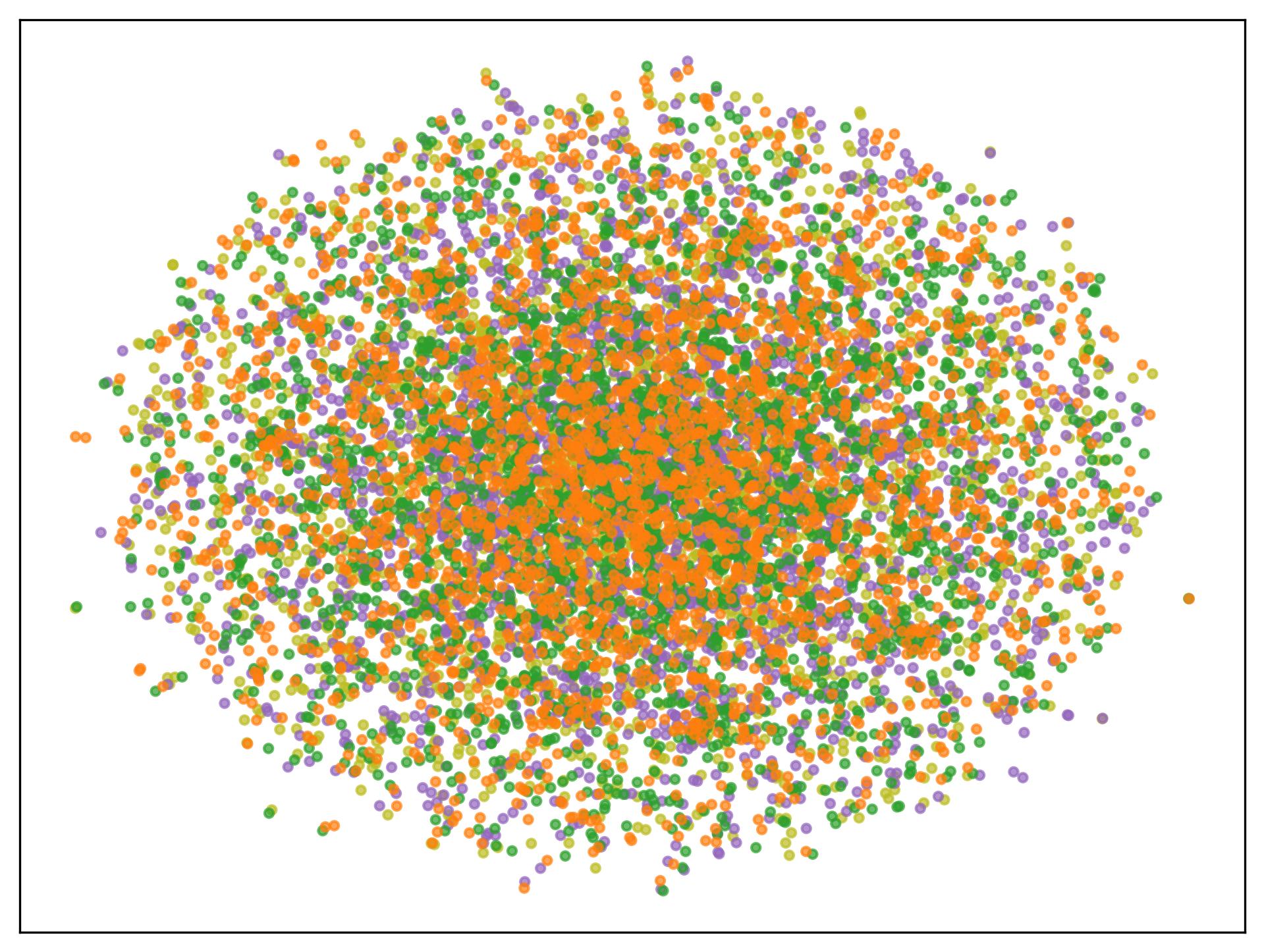
(a) I2E

(b) I2E${}_{\text{{proxy}}}$

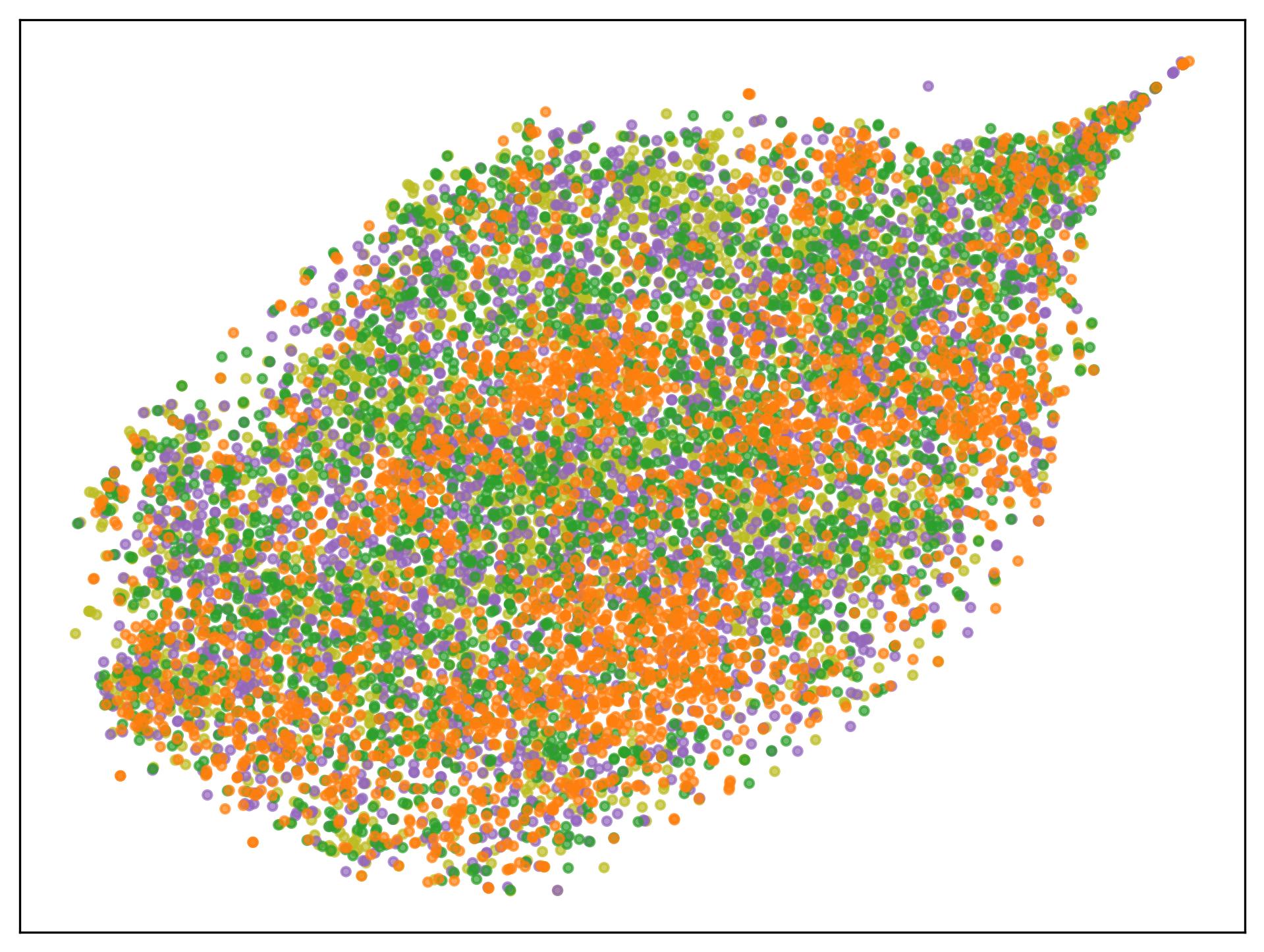
(c) VPL

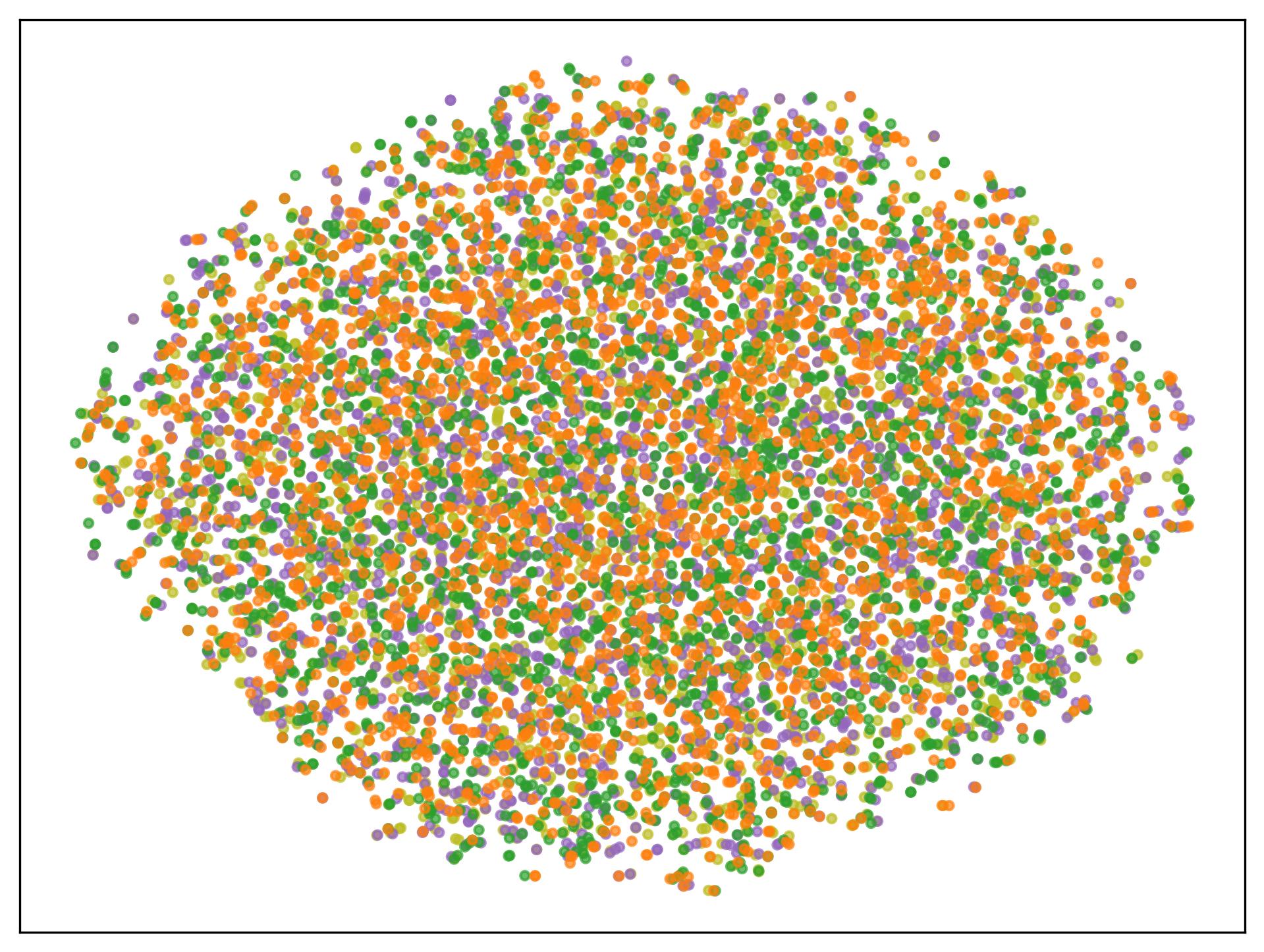
(d) PAL

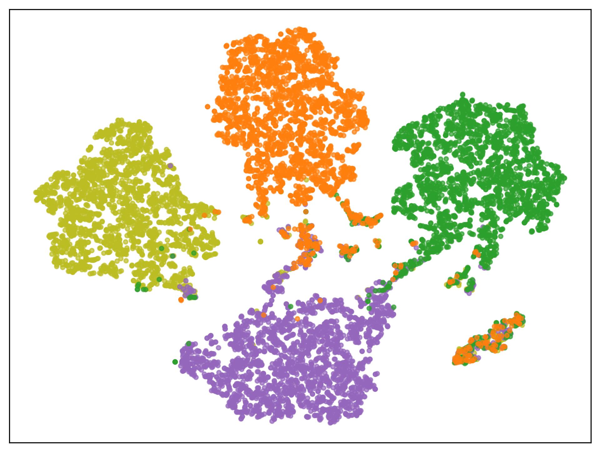
(e) CoPL

Figure 1: T-SNE visualization of seen user embeddings in UF-P-4-AVG with gemma-2b-it. Points are colored by their preference group. Our method clusters users in the same group more effectively, whereas other baselines fail to cluster users by their preference groups in user embedding space.

Since UF-P-4 encompasses a broader range of preferences, users provide more annotations to capture this added complexity. These configurations enable us to rigorously evaluate how reward models perform under sparse user annotations, a critical challenge for large-scale personalized alignment in practical settings.

Notably, our experimental environments remain consistent with previous work (Poddar et al., 2024), but more closely mirror our target environments. Specifically, Poddar et al. (2024) infers user preferences from a small, predefined pool of unannotated pairs, so all users must be evaluated within that limited query set. In contrast, we consider a much broader range of unannotated pairs, allowing the model to capture preferences across diverse contexts and better adapt to real-world personalized alignment scenarios.

Baselines.

We evaluate six baselines to benchmark. First, we use a uniform preference model (Uniform) trained on all annotations via BTL. Additionally, we consider four personalized reward models: I2E, I2E${}_{\text{{proxy}}}$ (Li et al., 2024), VPL (Poddar et al., 2024), and PAL Chen et al. (2024a). Finally, we include an Oracle, which has access to user group information and all annotations in the survey set and trains a separate reward function in Eq.˜1 for each preference group. The details of each model are provided in the Appendix˜B.

	Oracle	Uniform	I2E	I2E${}_{\text{{proxy}}}$	VPL	PAL	CoPL
Common	$71.86_{\pm 0.14}$	$\textbf{74.52}_{\pm 0.45}$	$73.94_{\pm 0.21}$	$74.15_{\pm 1.53}$	$72.73_{\pm 1.00}$	$70.82_{\pm 0.17}$	$71.23_{\pm 1.63}$
Controversial	$57.68_{\pm 0.27}$	$49.86_{\pm 0.30}$	$49.61_{\pm 0.05}$	$49.86_{\pm 0.06}$	$50.26_{\pm 0.44}$	$49.79_{\pm 0.12}$	$\textbf{56.89}_{\pm 1.56}$
Total	$64.53_{\pm 0.14}$	$61.82_{\pm 0.16}$	$61.48._{\pm 0.18}$	$61.59_{\pm 0.79}$	$61.11_{\pm 0.32}$	$59.95_{\pm 0.04}$	$\textbf{63.81}_{\pm 0.15}$

Table 2: Accuracy of reward models on UF-P-2-ALL with gemma-2b-it, broken down by pair type. Common refers to pairs for which the two preference groups provide the same preference label, Controversial refers to pairs labeled differently by the two groups, and Total encompasses all pairs. These categories reflect how diverse user preferences affect the performance of reward models. Bold represents the best result, except with Oracle.

Training and evaluation details.

For reward function training, we utilize two LLM backbones: gemma-2b-it and gemma-7b-it (Team et al., 2024). Our model uses one shared LoRA, eight LoRA experts, each with a rank of eight, and a two-layer MLP for the gating function. The other baselines, e.g., Uniform, I2E, VPL, PAL, and Oracle, use a LoRA rank of 64. Other training details, such as hyper-parameters and model architecture, are provided in Section˜C.2.

We report reward model accuracy on unseen test pairs that are not in the survey set. We define a correct prediction as assigning a higher score to the preferred response. We evaluate performance for both seen and unseen users. For seen user experiments, each user is assigned 10 test pairs, and accuracy is calculated over all seen users. We fix the number of unseen users at 100, evenly distributed across preference groups. To adapt the reward model for each unseen user, we provide 8 annotations in UF-P-2-ALL/AVG and 16 annotations in UF-P-4-ALL/AVG, followed by evaluation on 50 test pairs per unseen user. CoPL uses 2-hop neighbors for unseen user adaptation.

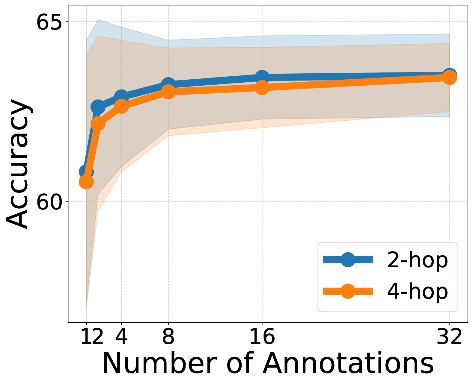
(a) UF-P-2-AVG

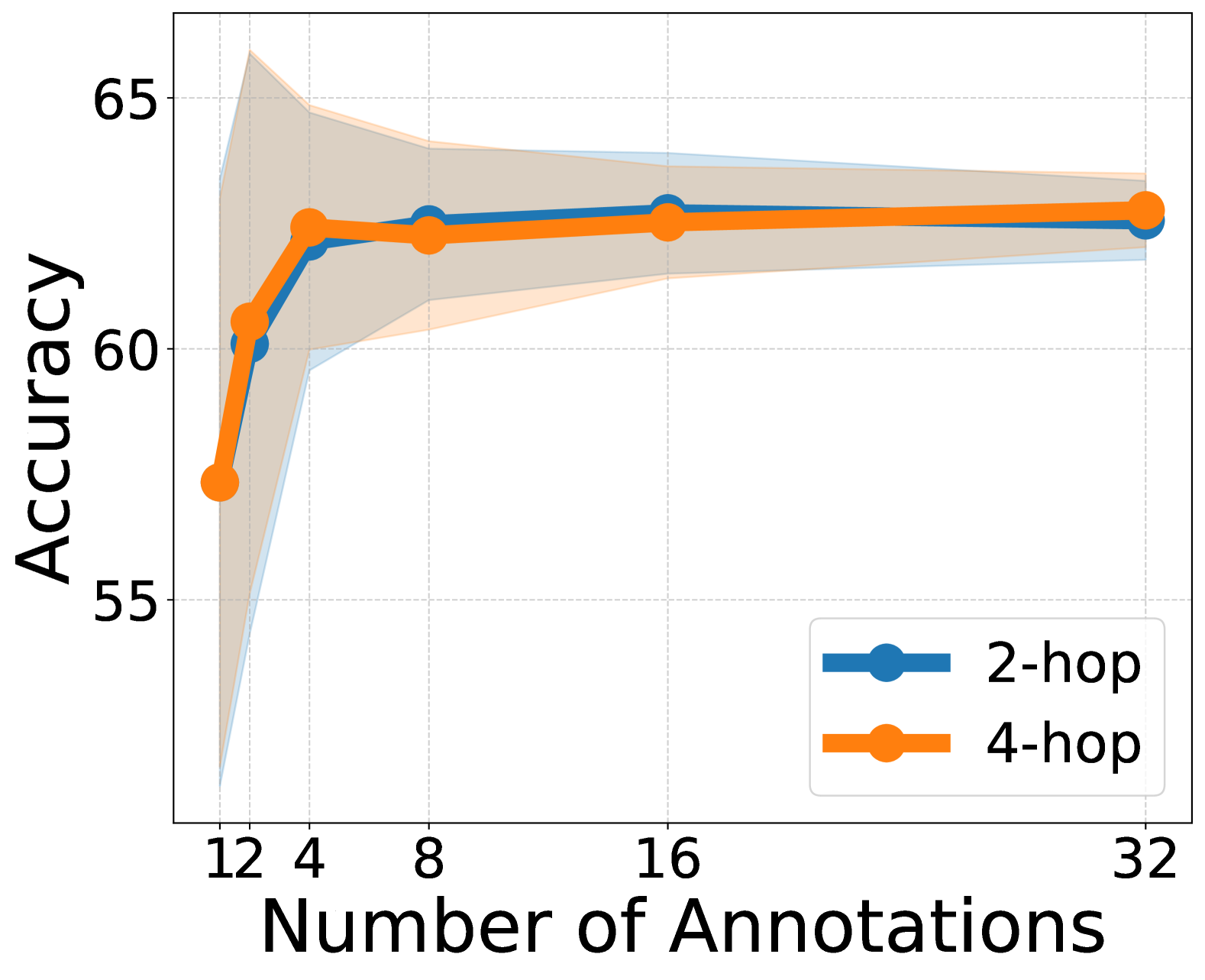
(b) UF-P-4-AVG

Figure 2: Accuracy of unseen user adaptation as the number of provided annotation sets increases, evaluated on UF-P-2/4-AVG with gemma-2b-it. 2-hop and 4-hop indicates 2-hop and 4-hop adaptation, respectively.

5.2 Results

Table˜1 presents accuracy for both seen and unseen users. CoPL consistently outperforms other baselines, except for Oracle, in both seen user and unseen user experiments. Notably, CoPL is comparable with Oracle in UF-P-4-ALL/AVG. In unseen user experiments, CoPL achieves accuracy comparable to the seen user setting, indicating the effectiveness of our unseen user adaptation.

Fig.˜1 visualizes the embedding space of seen users in UF-P-4-AVG, which is the most challenging environment in these experiments, and demonstrates that GNN-based representation learning can capture preference similarity between users even when each user provides few annotations.

5.3 Analysis

Analysis of performance in UF-P-2.

In Table˜1, all models appear capable of representing diverse preferences, surprisingly including the uniform models in UF-P-2-ALL/AVG. To investigate further, we divide the test pairs of UF-P-2 into common and controversial categories, where common pairs have identical annotations from both preference groups, and controversial pairs differ. Focusing on the seen user results in UF-P-2-ALL with gemma-2b-it from Table˜1, we break down the accuracy in Table˜2. The results indicate that baselines, except Oracle, struggle with controversial pairs, suggesting a tendency to capture only the common preference across all users. By contrast, our method achieves comparable performance to Oracle on controversial pairs while preserving high accuracy on common pairs.

Effect of the number of annotations in unseen user adaptation.

Fig.˜2 shows accuracy as the number of provided annotations increases in UF-P-2-AVG and UF-P-4-AVG. We observe that additional annotations lead to more accurate preference predictions for unseen users in general. However, in practice, even eight annotations are sufficient, enabling accurate inference of each user’s preference. We also compare two-hop and four-hop adaptations, but there is no significant difference.

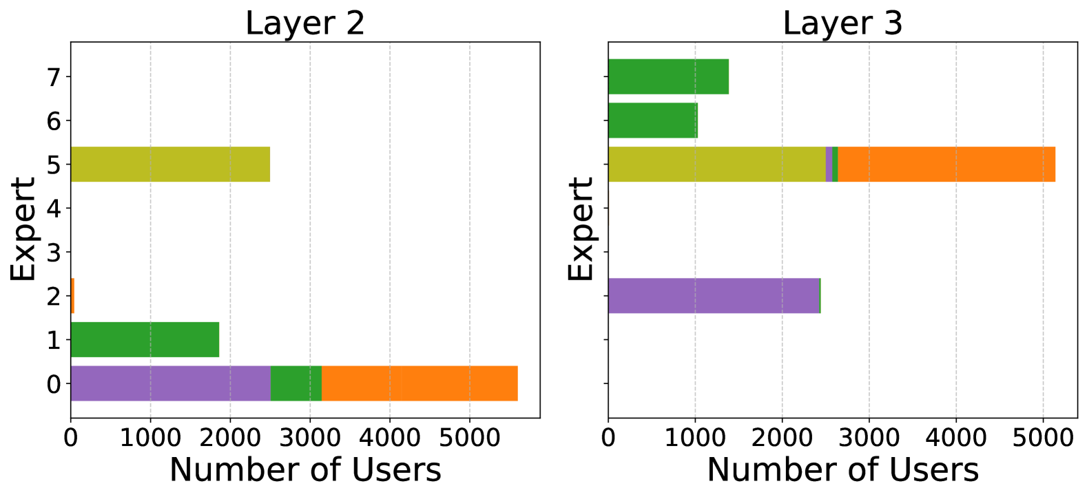
Figure 3: Expert allocation at layers 2 and 3 in UF-P-4-ALL with gemma-2b-it. Colors indicate preference groups. Users with similar preference groups are mapped to the same expert.

	UF-P-2-ALL	UF-P-4-ALL
CoPL	$\textbf{63.81}_{\pm 0.16}$	$\textbf{62.57}_{\pm 0.38}$
w/o GNN embedding	$62.09_{\pm 0.38}$	$56.75_{\pm 0.30}$
w/o MoLE $(n=64)$	$62.69_{\pm 0.86}$	$62.28_{\pm 0.33}$
w/o MoLE $(n=16)$	$62.43_{\pm 0.69}$	$62.13_{\pm 0.12}$

Table 3: Ablation study of CoPL in UF-P-2/4-ALL with gemma-2b-it. w/o GNN embedding replaces user embeddings from GNN with learnable user embeddings. w/o MoLE removes the MoLE and projects user embeddings into the token space. The symbol $n$ denotes the LoRA rank. All experiments run on three seeds.

Ablation study of CoPL.

Table˜3 presents an ablation study of CoPL, focusing on GNN-derived user embeddings and the MoLE architecture. When GNN embeddings are removed, user representations become learnable parameters. Without MoLE, user embeddings are projected into the token space and passed as an additional token to the reward model. The results indicate that components of CoPL are effective. Specifically, GNN-based embeddings are a crucial component of CoPL, and the MoLE architecture further enhances accuracy. Notably, CoPL uses fewer activated parameters than w/o MoLE $(n=64)$.

Fig.˜3 depicts expert allocation across layers two and three, where the user-conditioned gating mechanism partitions users differently at each layer. We can observe that users with the same preferences tend to be routed to the same expert.

	UF-P-4-ALL	UF-P-4-AVG
CoPL	$\textbf{61.62}_{\pm 0.10}$	$\textbf{61.97}_{\pm 0.35}$
Naive Avg.	$59.91_{\pm 0.59}$	$59.39_{\pm 0.50}$
User Opt.	$59.24_{\pm 0.71}$	$59.45_{\pm 0.72}$

Table 4: Accuracy of unseen-user adaptation in UF-P-4-ALL/AVG with gemma-2b-it. Naive Avg. computes the unseen user’s embedding as the unweighted average of 2-hop neighbors, while CoPL applies a weighted average strategy. User Opt. represents an optimization-based approach that learns a parameterized user embedding by maximizing the likelihood of the given annotations. All experiments run on three seeds.

Ablation study of unseen user adaptation.

We conduct an ablation study to evaluate the effectiveness of the unseen user adaptation strategy, comparing it to two baselines, Naive Avg and User Opt. Naive Avg assigns each unseen user embedding as the unweighted average of 2-hop seen user embeddings. User Opt replaces $e_{u}^{(L)}$ with a parameterized embedding learned by minimizing Equation (5) on the provided annotations. Table˜4 reports results in UF-P-4-ALL/AVG with gemma-2b-it, showing that CoPL outperforms both alternatives while achieving better computational efficiency than the optimization-based User Opt.

Fig.˜4 illustrates that naive averaging places unseen users away from identical preference group users, whereas our method clusters them more closely with users who share the same preferences.

UF-P-2		UF-P-4
ALL	AVG	ALL	AVG
$84.84_{\pm 0.83}$	$84.32_{\pm 0.09}$	$90.01_{\pm 0.35}$	$87.74_{\pm 0.19}$

Table 5: Test accuracy of the GNN. We evaluate the model using the same users from training but with annotation pairs that are not reflected in the graph. All experiments run on three seeds.

	UF-P-2-ALL	UF-P-4-ALL
CoPL	$63.81_{\pm 0.16}$	$62.57_{\pm 0.38}$
Pseudo label	$62.77_{\pm 0.70}$	$62.26_{\pm 0.27}$
Oracle	$64.53_{\pm 0.14}$	$61.52_{\pm 0.13}$
User-specific	$58.09_{\pm 1.73}$	$55.30_{\pm 3.30}$

Table 6: Accuracy of reward model trained by using a pre-trained GNN in UF-P-2/4-ALL with gemma-2b-it. The pseudo-label variant trains a reward model on all seen user–response pairs, with annotations provided by GNN-predicted labels. The user-specific variant refers to a BTL model trained with pseudo labels for each user. Only 10 users per group are sampled due to computational constraints. All experiments run on three seeds.

Training reward models with GNN.

Table˜5 reports GNN accuracy on seen users and responses for test pairs excluded from the training dataset. The results demonstrate that GNN can accurately predict labels for unannotated pairs with sparse annotations.

Table˜6 examines the impact of training with GNN-based pseudo labels, allowing the model to leverage additional preference data. Although the pseudo-labeled pairs increase the dataset size, performance is slightly worse than using only user-provided annotations, suggesting that noise degrades model accuracy.

To investigate the effect of noise further, a user-specific reward model is trained on pseudo labels for a random sample of 10 users per group. The results are considerably worse than the Oracle, indicating that noisy labels introduce training instability. This observation aligns with Wang et al. (2024), which notes that noisy preference labels can lead to training instability and performance degradation.

6 Conclusion

In this work, we introduced CoPL, a novel approach for personalizing LLMs through graph-based collaborative filtering and MoLE. Unlike existing methods that treat user preferences independently or require predefined clusters, our approach leverages multi-hop user-response relationships to improve preference estimation, even in sparse annotation settings. By integrating user-specific embeddings into the reward modeling process with MoLE, CoPL effectively predicts an individual preference.

Limitations

This work demonstrates how GCF-based user embeddings enable personalization in sparse settings, but we do not explore other GNN architectures that could further reduce sample complexity. Additionally, although CoPL employs a gating mechanism for user-specific expert allocation, we did not apply load-balancing loss, which induces more even activation among experts. As a result, some experts remain inactive in Fig.˜3. Future work may investigate different GNN designs and incorporate load-balancing techniques to fully leverage the potential of GNN and MoLE, respectively.

The oracle model may appear underwhelming, likely because our smaller backbone LLM struggles to capture subtle stylistic differences between responses. Larger-scale models (over 30B parameters) could better handle these nuances; however, constraints in our current setup prevent such experiments, and we defer them to future work.

Appendix

Appendix A Message Passing for Response Embeddings

Given user and response embeddings at layer $\ell$, a message from neighborhood users to the response as

$$m_{r}^{+}=\sum_{u\in\mathcal{N}^{+}_{r}}\alpha_{u,r}\Bigl{(}\hat{W}_{1}^{(\ell)}e_{u}^{(\ell)}+\hat{W}_{2}^{(\ell)}(e_{u}^{(\ell)}\odot e_{r}^{(\ell)})\Bigr{)},$$

$$m_{r}^{-}=\sum_{u\in\mathcal{N}^{-}_{r}}\beta_{u,r}\Bigl{(}\hat{W}_{3}^{(\ell)}e_{u}^{(\ell)}+\hat{W}_{4}^{(\ell)}(e_{u}^{(\ell)}\odot e_{r}^{(\ell)})\Bigr{)},$$

$$m^{(\ell)}_{r}=\hat{W}_{\text{self}}^{(\ell)}\,e_{r}^{(\ell)}\;+\;m_{r}^{+}\;+\;m_{r}^{-},$$ (12)

where $\hat{W}_{1}^{(\ell)},\hat{W}_{2}^{(\ell)},\hat{W}_{3}^{(\ell)},\hat{W}_{4}^{(\ell)},\hat{W}_{\text{self}}^{(\ell)}\in\mathbb{R}^{d\times d}$ are parameter matrices, $\odot$ is element-wise multiplication, and $\alpha_{u,r}$ and $\beta_{u,r}$ are normalization factors, set to $\frac{1}{\sqrt{|\mathcal{N}^{+}_{u}|\cdot|\mathcal{N}^{+}_{r}|}}$ and $\frac{1}{\sqrt{|\mathcal{N}^{-}_{u}|\cdot|\mathcal{N}^{-}_{r}|}}$, respectively.

Then, the response embedding is updated with the aggregated message $m^{(\ell)}_{r}$:

$$e_{r}^{(\ell+1)}={\psi}\bigl{(}m^{(\ell)}_{r}\bigr{)},$$ (13)

where $\psi(\cdot)$ is a non-linear activation.

Appendix B Method Baselines

Uniform.

The uniform model is a standard approach for pairwise preference comparisons. We train the uniform model with all annotation pairs, which will capture the common preference.

Oracle.

For an oracle model of our setting, we train the model with the true group membership of all users. A separate uniform model is trained for each group by aggregating annotations from the users in that group.

I2E (Li et al., 2024).

I2E is a framework that uses DPO to personalize LLM. However, it can be easily extended to reward modeling. I2E trains a model that maps the user index into a learnable embedding. It appends each user embedding as an additional input token to the LLM, providing user-specific signals for reward prediction.

I2E${}_{\text{proxy}}$ (Li et al., 2024).

A variant of I2E that introduces $N$ proxy embeddings. A weighted combination of these proxies forms the final user embedding, which is passed to the LLM for reward prediction. In our experiments, we use $N=10$.

VPL (Poddar et al., 2024).

Variational Preference Learning (VPL) encodes user-specific annotations into user embeddings. The user embeddings are then combined with sentence representations via an MLP to predict reward scores. To capture the user preferences effectively, VPL uses a variational approach that maps the user annotations into a prior distribution.

PAL (Chen et al., 2024a).

Pluralistic Alignment (PAL) applies an ideal-point model, where the distance between the user and the response determines the reward. The ideal point of the user is represented by $N$ proxies, set to $N=10$ in this work. Among variants of PAL, we use PAL-A with logistic loss.

Appendix C Experimental Details

In this section, we provide a detailed explanation of dataset construction and hyper-parameters.

C.1 Ultrafeedback-P

Poddar et al. (2024) proposes the Ultrafeedback-P (UF-P) benchmark for personalized reward modeling, based on the Ultrafeedback (UF) dataset Cui et al. (2023), which provides response pairs rated on four attributes: helpfulness, honesty, instruction following, and truthfulness. In UF-P, each attribute corresponds to a distinct preference. For instance, a user belonging to the helpfulness group annotates pairs, solely considering the helpfulness score.

UF-P-2.

This version employs only two attributes and removes pairs that both user groups label identically, focusing on controversial cases where preferences differ.

UF-P-4.

All four attributes are retained as preference dimensions, which allows for partial agreement among groups and hence increases complexity. Although Poddar et al. (2024) also excludes pairs fully agreed upon by all users, the remaining set is larger and exhibits more variety than UF-P-2.

In Poddar et al. (2024), each user is given a small context sample from a limited set of unannotated pairs to infer the user’s preference. In contrast, we leverage every available pair in the dataset to infer each user’s preferences. For our dataset construction, we use UF-P-4 dataset.

C.2 Hyper-parameters

We describe the training details of GNN, a reward model, and unseen user adaptation, such as model architecture and hyper-parameters.

GNN.

The model consists of four message-passing layers, each with user and response embeddings of dimension 512. We use Leaky ReLU as non-linear activation function to update user and response embeddings. Training proceeds for 300 epochs using the AdamW optimizer Loshchilov (2017) with a learning rate of $1\times 10^{-4}$ and a cosine scheduler with warmup ratio $0.1$. The batch size is 1024, and all experiments are conducted on an RTX 4090 GPU.

Reward models.

CoPL comprises an LLM backbone and a MoLE adapter. We use gemma-2b-it or gemma-7b-it as the LLM backbone. MoLE includes one shared expert and eight LoRA experts with a rank of eight. A two-layer MLP with a hidden dimension of 256 and ReLU activation serves as the gating mechanism, with a temperature set to 1.

We train the reward models using the AdamW optimizer with a learning rate of $5\times 10^{-5}$ and a cosine scheduler with warmup ratio $0.03$. Four GPUs, such as RTX6000ADA, L40S, and A100-PCIE-40GB, are employed with a batch size of 32 per GPU for gemma-2b-it and 16 per GPU for gemma-7b-it.

Baseline models use LoRA with rank 64. They also trained with an AdamW optimizer and a cosine scheduler with a warmup ratio $0.03$. We search the learning rate from $[1\times 10^{-4},5\times 10^{-5},1\times 10^{-5},5\times 10^{-6}]$.

User adaptation.

We use two-hop seen user and $0.07$ as temperature for unseen user adaptation of CoPL. For I2E, each learnable user representation is mapped into each user. For I2E${}_{\text{proxy}}$ and PAL, user representations are determined by $N=10$ proxies. Adapting to an unseen user requires parameter optimization for unseen users, typically through several gradient steps. To optimize the parameters for unseen users, 50 gradient steps are applied during adaptation.

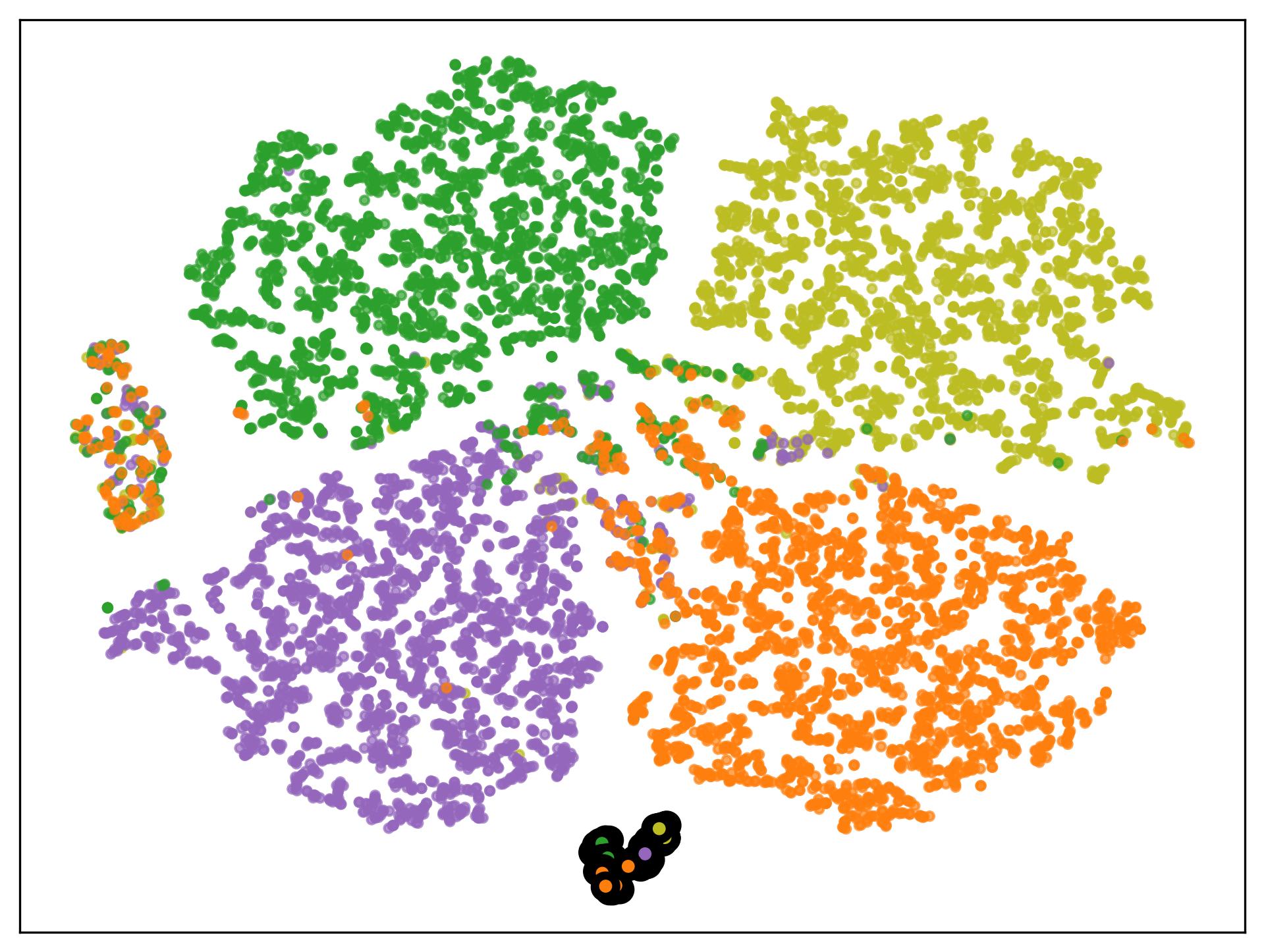
(a) Naive Avg.

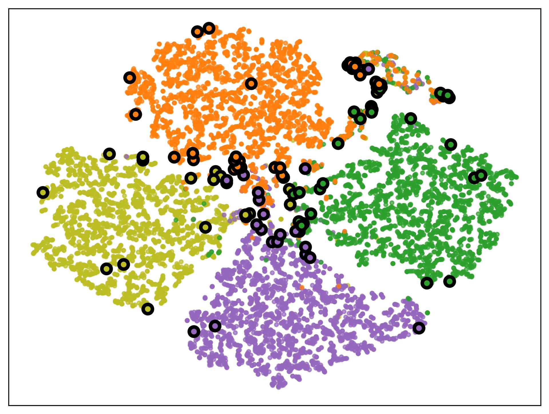
(b) User Opt.

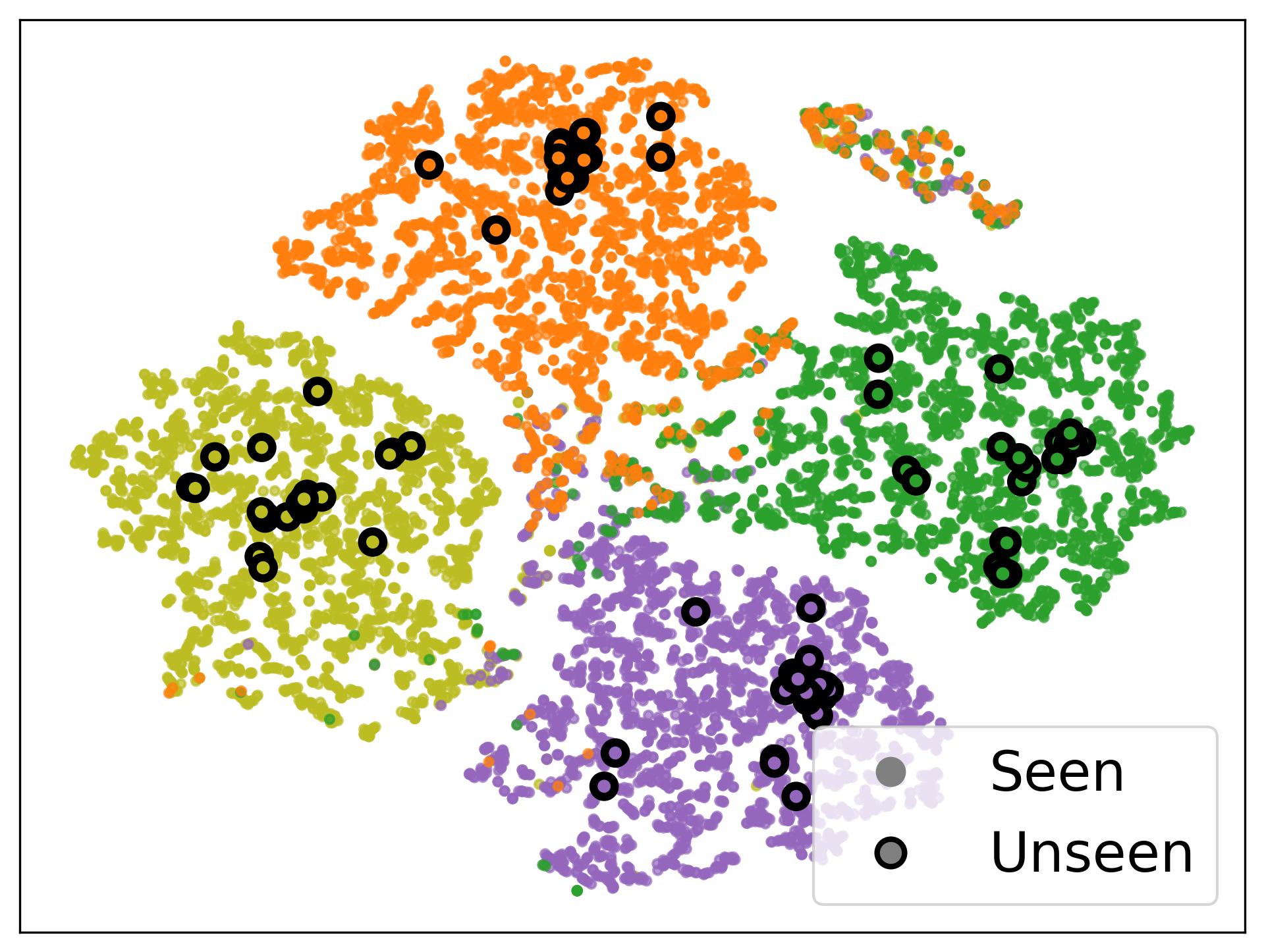
(c) CoPL

Figure 4: T-SNE visualization of seen and unseen user embeddings in UF-P-4-AVG. Naive Avg. computes unseen user embeddings as the unweighted mean of 2-hop neighbor embeddings. User Opt. represents an optimization-based approach that learns a parameterized user embedding by maximizing the likelihood of the given annotations. Colors indicate preference groups, and points with black edges represent unseen users. Unseen users adapted by our method align with their respective preference groups.

References

- Achiam et al. (2023) Josh Achiam, Steven Adler, Sandhini Agarwal, Lama Ahmad, Ilge Akkaya, Florencia Leoni Aleman, Diogo Almeida, Janko Altenschmidt, Sam Altman, Shyamal Anadkat, et al. 2023. Gpt-4 technical report. arXiv preprint arXiv:2303.08774.
- Bai et al. (2022) Yuntao Bai, Andy Jones, Kamal Ndousse, Amanda Askell, Anna Chen, Nova DasSarma, Dawn Drain, Stanislav Fort, Deep Ganguli, Tom Henighan, et al. 2022. Training a helpful and harmless assistant with reinforcement learning from human feedback. arXiv preprint arXiv:2204.05862.
- Bradley and Terry (1952) Ralph Allan Bradley and Milton E Terry. 1952. Rank analysis of incomplete block designs: I. the method of paired comparisons. Biometrika, 39(3/4):324–345.
- Chen et al. (2024a) Daiwei Chen, Yi Chen, Aniket Rege, and Ramya Korlakai Vinayak. 2024a. Pal: Pluralistic alignment framework for learning from heterogeneous preferences. Preprint, arXiv:2406.08469.
- Chen et al. (2020) Lei Chen, Le Wu, Richang Hong, Kun Zhang, and Meng Wang. 2020. Revisiting graph based collaborative filtering: A linear residual graph convolutional network approach. In Proceedings of the AAAI conference on artificial intelligence.
- Chen et al. (2024b) Lu Chen, Rui Zheng, Binghai Wang, Senjie Jin, Caishuang Huang, Junjie Ye, Zhihao Zhang, Yuhao Zhou, Zhiheng Xi, Tao Gui, et al. 2024b. Improving discriminative capability of reward models in rlhf using contrastive learning. In Proceedings of the 2024 Conference on Empirical Methods in Natural Language Processing, pages 15270–15283.
- Chen et al. (2024c) Shaoxiang Chen, Zequn Jie, and Lin Ma. 2024c. Llava-mole: Sparse mixture of lora experts for mitigating data conflicts in instruction finetuning mllms. arXiv preprint arXiv:2401.16160.
- Chen et al. (2023) Zeren Chen, Ziqin Wang, Zhen Wang, Huayang Liu, Zhenfei Yin, Si Liu, Lu Sheng, Wanli Ouyang, and Jing Shao. 2023. Octavius: Mitigating task interference in mllms via lora-moe. In ICLR.
- Cui et al. (2023) Ganqu Cui, Lifan Yuan, Ning Ding, Guanming Yao, Wei Zhu, Yuan Ni, Guotong Xie, Zhiyuan Liu, and Maosong Sun. 2023. Ultrafeedback: Boosting language models with high-quality feedback. Preprint, arXiv:2310.01377.
- Dai et al. (2023) Josef Dai, Xuehai Pan, Ruiyang Sun, Jiaming Ji, Xinbo Xu, Mickel Liu, Yizhou Wang, and Yaodong Yang. 2023. Safe rlhf: Safe reinforcement learning from human feedback. arXiv preprint arXiv:2310.12773.
- He and Chua (2017) Xiangnan He and Tat-Seng Chua. 2017. Neural factorization machines for sparse predictive analytics. Preprint, arXiv:1708.05027.
- He et al. (2020) Xiangnan He, Kuan Deng, Xiang Wang, Yan Li, Yongdong Zhang, and Meng Wang. 2020. Lightgcn: Simplifying and powering graph convolution network for recommendation. In Proceedings of the 43rd International ACM SIGIR conference on research and development in Information Retrieval, pages 639–648.
- Hu et al. (2021) Edward J Hu, Yelong Shen, Phillip Wallis, Zeyuan Allen-Zhu, Yuanzhi Li, Shean Wang, Lu Wang, and Weizhu Chen. 2021. Lora: Low-rank adaptation of large language models. arXiv preprint arXiv:2106.09685.
- Jang et al. (2023) Joel Jang, Seungone Kim, Bill Yuchen Lin, Yizhong Wang, Jack Hessel, Luke Zettlemoyer, Hannaneh Hajishirzi, Yejin Choi, and Prithviraj Ammanabrolu. 2023. Personalized soups: Personalized large language model alignment via post-hoc parameter merging. arXiv preprint arXiv:2310.11564.
- Li et al. (2022) Jiacheng Li, Tong Zhao, Jin Li, Jim Chan, Christos Faloutsos, George Karypis, Soo-Min Pantel, and Julian McAuley. 2022. Coarse-to-fine sparse sequential recommendation. In Proceedings of the 45th international ACM SIGIR conference on research and development in information retrieval, pages 2082–2086.
- Li et al. (2024) Xinyu Li, Zachary C Lipton, and Liu Leqi. 2024. Personalized language modeling from personalized human feedback. arXiv preprint arXiv:2402.05133.
- Lin et al. (2022) Zihan Lin, Changxin Tian, Yupeng Hou, and Wayne Xin Zhao. 2022. Improving graph collaborative filtering with neighborhood-enriched contrastive learning. In Proceedings of the ACM Web Conference 2022, WWW ’22, page 2320–2329, New York, NY, USA. Association for Computing Machinery.
- Liu et al. (2024) Qidong Liu, Xian Wu, Xiangyu Zhao, Yuanshao Zhu, Derong Xu, Feng Tian, and Yefeng Zheng. 2024. When moe meets llms: Parameter efficient fine-tuning for multi-task medical applications. In Proceedings of the 47th International ACM SIGIR Conference on Research and Development in Information Retrieval, SIGIR ’24. Association for Computing Machinery.
- Loshchilov (2017) I Loshchilov. 2017. Decoupled weight decay regularization. arXiv preprint arXiv:1711.05101.
- Molina et al. (2024) Ismael Villegas Molina, Audria Montalvo, Benjamin Ochoa, Paul Denny, and Leo Porter. 2024. Leveraging llm tutoring systems for non-native english speakers in introductory cs courses. arXiv preprint arXiv:2411.02725.
- Oh et al. (2024) Minhyeon Oh, Seungjoon Lee, and Jungseul Ok. 2024. Active preference-based learning for multi-dimensional personalization. Preprint, arXiv:2411.00524.
- Poddar et al. (2024) Sriyash Poddar, Yanming Wan, Hamish Ivison, Abhishek Gupta, and Natasha Jaques. 2024. Personalizing reinforcement learning from human feedback with variational preference learning. arXiv preprint arXiv:2408.10075.
- Rendle et al. (2012) Steffen Rendle, Christoph Freudenthaler, Zeno Gantner, and Lars Schmidt-Thieme. 2012. Bpr: Bayesian personalized ranking from implicit feedback. arXiv preprint arXiv:1205.2618.
- Shi et al. (2024) Jingzhe Shi, Jialuo Li, Qinwei Ma, Zaiwen Yang, Huan Ma, and Lei Li. 2024. Chops: Chat with customer profile systems for customer service with llms. arXiv preprint arXiv:2404.01343.
- Siththaranjan et al. (2024) Anand Siththaranjan, Cassidy Laidlaw, and Dylan Hadfield-Menell. 2024. Distributional preference learning: Understanding and accounting for hidden context in rlhf. In ICLR.
- Sorensen et al. (2024) Taylor Sorensen, Jared Moore, Jillian Fisher, Mitchell Gordon, Niloofar Mireshghallah, Christopher Michael Rytting, Andre Ye, Liwei Jiang, Ximing Lu, Nouha Dziri, et al. 2024. A roadmap to pluralistic alignment. arXiv preprint arXiv:2402.05070.
- Team et al. (2024) Gemma Team, Thomas Mesnard, Cassidy Hardin, Robert Dadashi, Surya Bhupatiraju, Shreya Pathak, Laurent Sifre, Morgane Rivière, Mihir Sanjay Kale, Juliette Love, et al. 2024. Gemma: Open models based on gemini research and technology. arXiv preprint arXiv:2403.08295.
- Venkatraman et al. (2024) Saranya Venkatraman, Nafis Irtiza Tripto, and Dongwon Lee. 2024. Collabstory: Multi-llm collaborative story generation and authorship analysis. arXiv preprint arXiv:2406.12665.
- Wang et al. (2024) Binghai Wang, Rui Zheng, Lu Chen, Zhiheng Xi, Wei Shen, Yuhao Zhou, Dong Yan, Tao Gui, Qi Zhang, and Xuan-Jing Huang. 2024. Reward modeling requires automatic adjustment based on data quality. In Findings of the Association for Computational Linguistics: EMNLP 2024, pages 4041–4064.
- Wang et al. (2019) Xiang Wang, Xiangnan He, Meng Wang, Fuli Feng, and Tat-Seng Chua. 2019. Neural graph collaborative filtering. In Proceedings of the 42nd international ACM SIGIR conference on Research and development in Information Retrieval, pages 165–174.
- Yang et al. (2024a) Kai Yang, Jian Tao, Jiafei Lyu, Chunjiang Ge, Jiaxin Chen, Weihan Shen, Xiaolong Zhu, and Xiu Li. 2024a. Using human feedback to fine-tune diffusion models without any reward model. In Proceedings of the IEEE/CVF Conference on Computer Vision and Pattern Recognition (CVPR), pages 8941–8951.
- Yang et al. (2024b) Rui Yang, Xiaoman Pan, Feng Luo, Shuang Qiu, Han Zhong, Dong Yu, and Jianshu Chen. 2024b. Rewards-in-context: Multi-objective alignment of foundation models with dynamic preference adjustment. arXiv preprint arXiv:2402.10207.