Nonparanormal Adjusted Marginal Inference

Dandl & Hothorn Nonparanormal Adjusted Marginal Inference Nonparanormal Adjusted Marginal Inference Treatment effects for assessing the efficacy of a novel therapy are typically defined as measures comparing the marginal outcome distributions observed in two or more study arms. Although one can estimate such effects from the observed outcome distributions obtained from proper randomisation, covariate adjustment is recommended to increase precision in randomised clinical trials. For important treatment effects, such as odds or hazard ratios, conditioning on covariates in binary logistic or proportional hazards models changes the interpretation of the treatment effect under non-collapsibility and conditioning on different sets of covariates renders the resulting effect estimates incomparable. We propose a novel nonparanormal model formulation for adjusted marginal inference allowing the estimation of the joint distribution of outcome and covariates featuring the intended marginally defined treatment effect parameter – including marginal log-odds ratios or log-hazard ratios. Marginal distributions are modelled by transformation models allowing broad applicability to diverse outcome types. Joint maximum likelihood estimation of all model parameters is performed. From the parameters not only the marginal treatment effect of interest can be identified but also an overall coefficient of determination and covariate-specific measures of prognostic strength can be derived. A free reference implementation of this novel method is available in R add-on package tram. For the special case of Cohen’s standardised mean difference $d$, we theoretically show that adjusting for an informative prognostic variable improves the precision of this marginal, noncollapsible effect. Empirical results confirm this not only for Cohen’s $d$ but also for log-odds ratios and log-hazard ratios in simulations and three applications. marginal effect, noncollapsibility, covariate adjustment, randomised trial, transformation model marginal effect, noncollapsibility, covariate adjustment, randomised trial, transformation model Susanne Dandl & Torsten Hothorn
Institut für Epidemiologie, Biostatistik und Prävention
Universität Zürich
Hirschengraben 84, CH-8001 Zürich, Switzerland
Email: Susanne.Dandl@uzh.ch

1 Introduction

Randomised clinical trials (RCTs) aim at the estimation of causally interpretable treatment effects. Typically, treatment effect parameters are defined as functions of marginal outcome distributions. In the simplest case, one compares the distributions of the outcome observed in two groups of patients: those randomised to be treated by a standard therapy and those randomised to receive an innovative therapy. For ease of communication and comparability between trials, treatment effects are expressed as differences in means, odds ratios, risk differences, hazard ratios, restricted mean survival times or similar marginally defined measures.

Increasing the precision of treatment effect estimates has kept statisticians on their toes over the last century. Two simple yet important ideas are stratification and covariate adjustment, both relying on the availability of prognostic information. Prognostic variables are baseline (or pre-treatment) covariates that are associated with the outcome and explain outcome heterogeneity. By exploiting the information in such prognostic variables, the precision of the treatment effect can be increased, leading to narrower confidence intervals and, therefore, more powerful inference about the true treatment effect.

Many classical contributions advocating for covariate adjustment in RCTs base their arguments on differences in means in analysis of covariance (ANCOVA) models (see Senn et al., 2024, and the references therein). The error term in such models accounts for some forms of model misspecification (such as missing or incorrectly transformed prognostic variables). Adding or removing terms only affects the variance of the residual term but not the model parameter corresponding to the average treatment effect. More flexible model formulations extending ANCOVA models (see, for example, the references in Siegfried et al., 2023) gained novel interest in the machine learning era (Schuler et al., 2022). Covariate adjustment has been recommended for the analysis of RCTs by several authorities (e.g., European Medicines Agency EMA/CHMP/295050/2013 and Food and Drug Administration FDA-2019-D-0934).

For nonnormal models, such as binary logistic or Cox models, lack of an explicit residual term introduces a dependency of the treatment effect parameter on unadjusted outcome heterogeneity. Adding prognostic variables to reduce the error variance leads to stronger treatment effects, i.e., higher effect magnitudes compared to the effect estimate of an unadjusted model. While this leads to increased power for null hypothesis significance tests of the treatment effects, the treatment effect estimates are not directly comparable between models with differing sets of prognostic covariates (see Robinson and Jewell, 1991; Martinussen and Vansteelandt, 2013; Daniel et al., 2021, among many others). In the literature, this noncomparability issue is also known as noncollapsibility. A treatment effect is called noncollapsible if the marginal effect obtained from averaging over the prognostic variables in a conditional model adjusting for variables is not identical to the effect obtained from a marginal model not adjusting for covariates (Aalen et al., 2015).

As alternatives to the simple remedy of reporting marginal and adjusted (“multivariable”) treatment effect estimates side-by-side in the presence of noncollapsibility, two conceptually different strategies were proposed. Strategy I is to replace the noncollapsible model by a collapsible one. An example is to replace the Cox proportional hazards model by a Weibull accelerated failure time model (Aalen et al., 2015) or to reformulate the treatment effect, for example as restricted mean survival times or risk differences. In this context, several generally applicable inference procedures have been suggested, most prominently G-computation or standardisation (Daniel et al., 2021; Van Lancker et al., 2024b).

Strategy II is to directly adjust marginal log-odds or log-hazard ratios for prognostic covariates. A framework for semiparametric locally efficient adjustment based on the joint distribution of outcome, treatment, and covariates was suggested by Tsiatis et al. (2008). The approach was generalised to marginal binary logistic regression models by Zhang et al. (2008), allowing inference on log-odds ratios, and to proportional hazards models by Lu and Tsiatis (2008), allowing inference on log-hazard ratios. Recently, Ye et al. (2024) applied very similar ideas to covariate adjustment for the comparison of marginal survivor curves, potentially also under proportional hazards. The advantage of this strategy is the marginal interpretability on classical log-odds or log-hazard ratio scales (Doi et al., 2022).

In the spirit of strategy II, we present a novel nonparanormal model featuring a marginal treatment effect parameter along with an estimation procedure able to leverage prognostic information for increasing the precision of corresponding treatment effect parameter estimates. For example, the novel nonparanormal adjusted marginal inference method suggested here allows to estimate a marginal log-odds ratio whose standard error shrinks with increasing strengths of available prognostic information. Using nonparanormal adjusted marginal inference, we are able to report interpretable and comparable marginal treatment effect estimates with smaller standard errors compared to an unadjusted analysis, even when the parameter is classified as being noncollapsible in conventional terminology (Van Lancker et al., 2024a).

On a more technical level, one can understand our contribution as a nonparanormal alternative to the semiparametric approach for the joint distribution of outcome, treatment, and covariates. Instead of leaving most aspects of this joint distribution unspecified (as done by Zhang et al., 2008), we suggest to model the joint distribution of outcome and covariates by a nonparanormal model (Liu et al., 2009). The marginal model for the outcome features the treatment effect parameter of interest, marginal covariate distributions are described in a model-free way, and their joint distribution is characterised by a Gaussian copula. This model gives rise to a novel formulation of the conditional distribution of outcome given treatment and covariates which is, by design, collapsible. The approach is based on marginal transformation models allowing broad definitions of marginal treatment effects, such as Cohen’s standardised differences in means $d$, odds and hazard ratios, probabilistic indices and other noncollapsible treatment effect parameters (Hothorn et al., 2018). The nonparanormal model is fully parameterised (exploiting connections to multivariate transformation models proposed by Klein et al., 2022) and thus standard maximum likelihood approaches in these models (Hothorn, 2024) can be applied for parameter estimation and the construction of confidence intervals or test procedures. This does not only apply to the marginal treatment effect, but also to prognostic covariate effects. Unlike semiparametric approaches, where the prognostic value of covariates is not directly quantified, our model provides an overall coefficient of determination as well as covariate-specific measures of prognostic strength.

We proceed by introducing the general concept for nonparanormal adjusted marginal inference and its application to the improved estimation of Cohen’s $d$ for continuous, odds ratios for binary, and hazard ratios for survival outcomes in Section 2. For the special case of Cohen’s $d$, we present an analytic expression of the standard error under covariate adjustment allowing to investigate the potential for sample size reductions theoretically. We evaluate the ability of nonparanormal adjusted marginal inference to increase precision in marginal treatment effect parameter estimation and to assess prognostic strength empirically for RCTs with continuous, binary, and survival outcomes in Sections 3 and 4.

2 Nonparanormal adjusted marginal inference

We are interested in the effect of some binary treatment $W\sim B(1,\pi)$ on the distribution of an outcome $Y\in\mathcal{Y}$ assuming an at least ordered sample space $\mathcal{Y}$. The propensity score $\pi=\mathbb{P}(W=1)$ is constant and does not rely on covariates in this randomised trial setting. In addition to $Y$ and $W$, $J-1$ baseline covariates $\text{\boldmath$X$}=(X_{1},X_{2},...,X_{J-1})$ were observed, with $X_{j}\in\mathcal{X}_{j},j=1,...,J-1$ assuming all covariate sample spaces $\mathcal{X}_{j}$ are at least ordered.

2.1 Univariate marginal and conditional transformation models

We denote the conditional cumulative distribution function of $Y$ given $W=0$ (“control”) as $F_{0}(y)=\mathbb{P}(Y\leq y\mid W=0)$ and the conditional cumulative distribution function of $Y$ given $W=1$ (“treated”) as $F_{1}(y)=\mathbb{P}(Y\leq y\mid W=1)$. The treatment effect $\tau:=\tau(F_{0},F_{1})\in\mathbb{R}$ expresses the discrepancy between the two marginal (with respect to covariates) distributions as an, ideally interpretable, scalar. Because $F_{0}$ and $F_{1}$ do not rely on covariates $X$, $F_{0}$ and $F_{1}$ are also called marginal models and $\tau$ reflects a marginal treatment effect. In randomised trials, it is possible to estimate $\tau$ from $Y$ and $W$ alone, ignoring covariates.

The two distribution functions $F_{0}$ and $F_{1}$ could be estimated nonparametrically, e.g., as empirical distribution functions without assuming a specifically distributional form, however, the characterisation of the discrepancy between the two distributions in the form of an interpretable scalar treatment effect $\tau$ is somewhat challenging. Alternatively, parametric distributions for $F_{0}$ and $F_{1}$ allow specification of interpretable treatment effects $\tau$, however, at the price of imposing strong assumptions on how the outcome distribution.

Transformation models (in the sense of Box and Cox, 1964; Hothorn et al., 2018) offer a compromise between the nonparametric and parametric world by transforming outcomes via a monotone nondecreasing transformation function $h:\mathcal{Y}\rightarrow\mathbb{R}$ such that the transformed outcome distribution is described by a simple cumulative distribution function $G:\mathbb{R}\rightarrow[0,1]$ with parameter-free log-concave absolute continuous density. This results in $F_{0}(y)=G(h(y))$ for the distribution under control. Throughout this manuscript, we assume that the treatment effect $\tau$ is defined as a shift effect on the scale of the transformation, i.e., $F_{1}(y)=G(h(y)-\tau)$, resulting in the overall marginal transformation model for the conditional distribution of the outcome $Y$ given treatment group $W=0$ or $W=1$ as

$$F_{w}(y)=F(y\mid W=w)=G(h(y)-\tau w)=G(h(y\mid w)).$$ (1)

Different choices of $G$ and $h$ to be discussed in Section 2.3 give rise to numerous classical and novel treatment effects $\tau$ for continuous, binary, ordered categorical, or survival outcomes $Y$.

Leveraging the prognostic information about the outcome $Y$ contained in the covariates $X$ is possible in linear transformation models with additional linear predictor $\tilde{\text{\boldmath$x$}}^{\top}\text{\boldmath$\beta$}$. In such models, the conditional cumulative distribution function of the outcome given treatment and covariates is formulated as

$$F(y\mid W=w,\text{\boldmath$X$}=\text{\boldmath$x$})=G(h_{\text{\boldmath$x$}}(y)-\tau_{\text{\boldmath$x$}}w-\tilde{\text{\boldmath$x$}}^{\top}\text{\boldmath$\beta$})$$ (2)

for some appropriate coding $\tilde{\text{\boldmath$x$}}$ of covariates $x$. In the following, we call the treatment effect parameter $\tau_{\text{\boldmath$x$}}$ the conditional effect to reflect that it is the effect when conditioning on covariates $X$. In general, the conditional effect $\tau_{\text{\boldmath$x$}}$ is not equal to the marginal effect $\tau$ in model (1), the same holds for the transformation functions $h$ and $h_{\text{\boldmath$x$}}$. If integrating the conditional model over the distribution of $X$ results in model (1), the effect $\tau$ is called collapsible (see Chapter 6 in Pearl, 2009, for a more general definition of collapsibility). Section 2.3 shows that Cohen’s $d$ in the linear model, the log-odds ratio in a binary logistic regression model, and the log-hazard ratio in the Cox model can be expressed as parameter $\tau$ in model (1). The corresponding conditional models are noncollapsible, that is, $\tau\neq\tau_{\text{\boldmath$x$}}$.

We proceed by proposing a model for the joint distribution of outcome given treatment and covariates by means of a Gaussian copula. The marginal outcome distribution $F_{w}(y)$ stays intact, allowing estimation of the marginal treatment effect $\tau$ in the presence of covariates. The model gives rise to a novel conditional distribution $F(y\mid W=w,\text{\boldmath$X$}=\text{\boldmath$x$})$ featuring the treatment effect $\tau$ in a collapsible way.

2.2 Multivariate transformation models

Transformation models for multivariate outcomes were introduced by Klein et al. (2022). These models extend univariate transformation models for a single $Y$ to situations where the joint distribution of multiple variables shall be modelled. We adapt this approach and treat the covariates $X$ as additional outcomes in a joint model for $(Y,\text{\boldmath$X$})$. We first parameterise the marginal covariate distributions as unconditional transformation models, i.e.,

$$\mathbb{P}(X_{j}\leq x_{j})=\Phi(h_{j}(x_{j})),j=1,...,J-1$$ (3)

with $h_{j}:\mathcal{Y}_{j}\rightarrow\mathbb{R}$ serving as the nondecreasing transformation function for $X_{j}$ and $\Phi$ denoting the cumulative distribution function of the standard normal. The outcome $Y$ is also transformed to a latent normal scale via $h_{J}(y\mid w):=\Phi^{-1}\left(G\left(h\left(y\mid w\right)\right)\right)$ based on model (1). The standard normal distribution function $\Phi$ is attractive as it provides a direct link to Gaussian copulas (Song et al., 2009) and nonparanormal models (Liu et al., 2009).

The multivariate transformation function $\text{\boldmath$h$}:\mathcal{X}_{1}\times\mathcal{X}_{2}\times\cdots\times\mathcal{X}_{J-1}\times\mathcal{Y}\rightarrow\mathbb{R}^{J}$ defined as $\text{\boldmath$h$}(\text{\boldmath$X$},Y\mid W=w)=\left(h_{1}(X_{1}),h_{2}(X_{2}),...,h_{J-1}(X_{J-1}),h_{J}(Y\mid w)\right)^{\top}$ formulates the joint cumulative distribution function of covariates $X$ and outcome $Y$ given treatment $W$ as

$$\mathbb{P}(Y\leq y,\text{\boldmath$X$}\leq\text{\boldmath$x$}\mid W=w)=\mathbb{P}(\text{\boldmath$X$}\leq\text{\boldmath$x$},Y\leq y\mid W=w)=\Phi_{\mathbf{\Sigma}}\left(\text{\boldmath$h$}(\text{\boldmath$x$},y\mid W=w)\right).$$ (4)

Here, $\Phi_{\mathbf{\Sigma}}$ denotes the cumulative distribution function of $\operatorname{N}_{J}(\mathbf{0},\mathbf{\Sigma})$, the $J$-dimensional normal distribution with zero mean and $J\times J$ correlation matrix $\mathbf{\Sigma}$ ensuring identifiability of $h$.

Based on Hothorn (2024), we parameterise the correlation matrix $\mathbf{\Sigma}$ in terms of the inverse of its Cholesky factor, that is, using the factorisation $\mathbf{\Sigma}=\mathbf{\Omega}^{-1}\mathbf{\Omega}^{-\top}$. The lower triangular $J\times J$ matrix $\mathbf{\Omega}=(\omega_{j\jmath})$ has positive diagonals $\omega_{jj}>0,j=1,\dots,J$ and lower triangular elements $\omega_{j\jmath},1\leq\jmath\leq j\leq J$. We write $\mathbf{\Omega}(\text{\boldmath$\lambda$})$ with unconstraint parameters $\text{\boldmath$\lambda$}=(\lambda_{21},\dots,\lambda_{J,J-1})^{\top}\in\mathbb{R}^{\nicefrac{{J(J-1)}}{{2}}}$ as the lower triangular elements of a unit lower triangular matrix

$$\mathbf{\Lambda}=\mathbf{\Lambda}(\text{\boldmath$\lambda$})=\left(\lambda_{jj^{\prime}}\right)_{1\leq j^{\prime}<j\leq J}$$ (5)

such that $\mathbf{\Omega}(\text{\boldmath$\lambda$})=\mathbf{\Lambda}(\text{\boldmath$\lambda$})\operatorname{diag}(\mathbf{\Lambda}^{-1}(\text{\boldmath$\lambda$})\mathbf{\Lambda}^{-\top}(\text{\boldmath$\lambda$}))^{1/2}$ in accordance with Section 2, Option 2 in Hothorn (2024). The corresponding precision matrix is $\mathbf{\Sigma}^{-1}=\mathbf{\Omega}^{\top}\mathbf{\Omega}$ and we refer to the correlations, on a latent transformed normal scale, between covariate $X_{j}$ and outcome $Y$ in both treatment groups, as the elements $\rho(\text{\boldmath$\lambda$})_{Jj},j=1,\dots,J-1$, of the last row of the correlation matrix $\mathbf{\Sigma}$. From the joint distribution of $Y$ and $X$ given treatment $W$ in model (4), we can derive the conditional distribution of $Y$ given $W$ and covariates $\text{\boldmath$X$}\subseteq\mathbb{R}^{J-1}$ from an absolute continuous distribution as

$$\mathbb{P}(Y\leq y\mid W=w,\text{\boldmath$X$}=\text{\boldmath$x$})=\Phi\left(\sum\limits_{j=1}^{J-1}\omega_{Jj}h_{j}(x_{j})+\omega_{JJ}h_{J}(y\mid w)\right).$$ (6)

The regression coefficients are obtained from the $J$th row of the precision matrix $\mathbf{\Sigma}^{-1}=\mathbf{\Omega}^{\top}\mathbf{\Omega}$, which is identical to the vector $\omega_{JJ}(\omega_{J1},\dots,\omega_{JJ})^{\top}$. It should be noted that the marginal model of $Y$ given $W$ is identical to model (1), i.e., $F_{w}(y)=\mathbb{P}(Y\leq y\mid W=w)=\Phi(h_{J}(y\mid w))=\Phi(\Phi^{-1}(G(h(y\mid w))))=G(h(y)-\tau w)$ because the model is constraint to unit marginal variances in $\mathbf{\Sigma}$. For absolute continuous $(Y,\text{\boldmath$X$})$, we can write the marginal model as $h_{J}(Y\mid w)=\varepsilon\sim\operatorname{N}(0,1)$ and the conditional distribution (6) is equivalent to a normal linear regression model for gaussianised outcome and covariates. With regression coefficients $-\omega_{JJ}^{-1}\omega_{Jj}$ for $h_{j}(x_{j}),j=1,\dots,J-1$ and residual standard deviation $\omega_{JJ}^{-1}$ we have

$$h_{J}(Y\mid w)=\sum_{j=1}^{J-1}-\omega_{JJ}^{-1}\omega_{Jj}h_{j}(x_{j})+\omega_{JJ}^{-1}\varepsilon.$$

Because $\mathbb{V}(h_{j}(X_{j}))=1$ for all $j=1,\dots,J-1$ by definition, we can rank covariates with respect to their prognostic strengths $|\omega_{Jj}|$. The gain obtained from adjusting for covariates can be measured by the coefficient of determination $R^{2}:=1-\omega_{JJ}^{-2}$ defined by the ratio of the residual variances $\omega_{JJ}^{-2}$ of the conditional model (6) and the marginal model with residual standard deviation one. For noncontinuous variables, the same arguments hold on a latent continuous scale.

2.3 Specific model applications

The choice of $G$ and $h$ depends on the outcome at hand and the desired interpretation of the treatment effect $\tau$. We follow Hothorn et al. (2018) and parameterise $h:\mathcal{Y}\rightarrow\mathbb{R}$ as a linear combination of basis functions, i.e.

$$h(y)=\text{\boldmath$a$}(y)^{\top}\text{\boldmath$\vartheta$}.$$ (7)

Here, $\text{\boldmath$a$}:\mathcal{Y}\rightarrow\mathbb{R}^{M}$ denotes a multi-dimensional basis function with $M\in\mathbb{N}$ while $\vartheta$ corresponds to basis coefficients. In the following, different choices of $G$, $a$ and $\vartheta$ are discussed for continuous, binary and survival outcomes. These choices give rise to various notions of treatment effects $\tau$, for example in terms of Cohen’s $d$, probabilistic indices, log-odds ratios, or log-hazard ratios. It is also shown how popular models, like the (proportional odds) logistic regression models or Cox proportional hazards models, can be embedded in our methodology. Appropriate choices for the transformations $h_{j},j=1,...,J-1$ for covariates in $X$ as well as parameter estimation for model (4) are discussed in Section 2.4. An attractive choice for $G$ in case of continuous outcomes is the standard normal distribution, i.e., $G=\Phi$. In the following, we discuss suitable choices for $h$ when the outcome is normally distributed and when this is not the case.

If the outcome $Y$ is normally distributed, a linear transformation function $h(y)=\vartheta_{1}+\vartheta_{2}y$ can be chosen, resulting in a classical linear model. The basis functions and parameters in model (7) are then equal to $\text{\boldmath$a$}(y)=(1,y)^{\top}$ and $\text{\boldmath$\vartheta$}=(\vartheta_{1},\vartheta_{2})^{\top}$. The parameterisations $Y\mid W=0\sim\operatorname{N}(-{\vartheta_{1}}\vartheta_{2}^{-1},\vartheta_{2}^{-2})$ and $Y\mid W=1\sim\operatorname{N}(-{(\vartheta_{1}-\tau)}\vartheta_{2}^{-1},\vartheta_{2}^{-2})$ lead to the marginal model

$$F_{w}(y)=\Phi\left(\vartheta_{1}+\vartheta_{2}y-\tau w\right).$$ (8)

The treatment effect $\tau$ is defined as the standardised difference in means – also known as Cohen’s $d$ – since $\E(Y\mid W=1)-\E(Y\mid W=0)=\tau\vartheta_{2}^{-1}$. Cohen’s $d$ is a noncollapsible effect measure: If more of the variance of $Y$ is explained by adding a prognostic covariate $X_{j}$ to the model, the conditional effect is larger than the marginal one. For normally distributed outcomes, a closed form expression of the standard error of Cohen’s $d$ in an unadjusted analysis can be derived.

Lemma 1.

Standard error of Cohen’s $d$ without covariate adjustment
In the model $Y\mid W=w\sim\operatorname{N}(-(\vartheta_{1}-\tau w)\vartheta_{2}^{-1},\vartheta_{2}^{-2})$ with Cohen’s $d$ denoted as $\tau$, the unadjusted standard error for $\tau$ in a balanced trial with total sample size $N$ is $\text{SE}(\tau)=\sqrt{\frac{2}{N}\left(\frac{\tau^{2}}{4}+2\right)}.$

The standard error for Cohen’s $d$ obtained from an analysis adjusting with respect to a single normally distributed covariate $X_{1}$ using the multivariate transformation model is also available in closed form.

Lemma 2.

Standard error of Cohen’s $d$ under covariate adjustment
If $Y\mid W=w\sim\operatorname{N}(-(\vartheta_{11}-\tau w)\vartheta_{12}^{-1},\vartheta_{12}^{-2})$ and $X_{1}\sim\operatorname{N}(-\vartheta_{21}\vartheta_{22}^{-1},\vartheta_{22}^{-2})$ whose joint distribution is given by a Gaussian copula with correlation $\rho=-\nicefrac{{\lambda}}{{\sqrt{1+\lambda^{2}}}}$, where $\lambda:=\lambda_{21}$ is the single unconstrained copula parameter in (5), the adjusted standard error for $\tau$ in a balanced trial with total sample size $N$ is $\text{SE}(\tau,\lambda)={\sqrt{\frac{2}{N}\left({(1+\lambda^{2})\tau^{2}+(2+\lambda^{2})4}\over{2\,\lambda^{4}+6\,\lambda^{2}+4}\right)}}.$

Proofs for both Lemmata are provided in Appendix A. The ratio of the squared standard errors can be interpreted as the fraction of the sample size of the unadjusted analysis that is required to achieve the same power in an adjusted analysis. Relevant reductions of more than $25\%$ can be gained when a single prognostic covariate with a correlation of $0.5$ with the outcome can be incorporated in the nonparanormal adjusted marginal inference procedure proposed here (Figure  S. 1 in Appendix A). The standard error $\text{SE}(\hat{\tau})$ is not always larger than the standard error $\text{SE}(\hat{\tau},\hat{\lambda})$ because the unadjusted marginal and the adjusted marginal parameter estimates typically differ slightly. However, $\text{SE}(\tau,\lambda)$ is monotonically decreasing with increasing values of $\mid\lambda\mid$ and thus prognostic strength of $X_{1}$.

The normal assumption is rarely met in practice and can be relaxed by allowing more flexible transformation functions $h$ and $h_{j}$. Hothorn et al. (2018) identified polynomials in Bernstein form of order $M$ as a suitable choice since they approximate any function over a closed interval for a sufficiently large $M$ according to Weierstrass’ approximation theorem (Farouki, 2012). Under $G=\Phi$ and a flexible, potentially nonlinear $h$, the interpretation of $\tau$ is not in terms of Cohen’s $d$ but as the mean difference on the latent normal scale. To obtain an effect interpretation that is more intuitive, $\tau$ can be transformed to a probabilistic index $\mathbb{P}(Y_{0}<Y_{1})=\Phi(\nicefrac{{\tau}}{{\sqrt{2}}})$, where $Y_{0}$ is defined as the outcome under $W=0$ and $Y_{1}$ as an independent outcome under $W=1$.

For the multivariate transformation model, no further transformation of $Y$ in the standard normal world is required since we assume that this already happened in the marginal model using $h$. The conditional distribution of $Y$ given $W$ and continuous $X$ is then given by

$$\mathbb{P}(Y\leq y\mid W=w,\text{\boldmath$X$}=\text{\boldmath$x$})=\Phi\left(\sum_{j=1}^{J-1}\omega_{Jj}h_{j}(x_{j})+\omega_{JJ}\left(h(y)-\tau w\right)\right).$$ (9)

By design, the treatment effect $\tau$ is collapsible in this conditional model: Integrating over covariates $X_{1},\dots,X_{J-1}$ via the joint Gaussian copula model produces the marginal model (1) featuring $\tau$. The conditional distribution function (9) is identical to the one implemented by the linear transformation model (2) when all covariates are jointly normal (with linear transformation functions $h_{j},j=1,\dots,J-1$); the noncollapsible conditional treatment effect is given by $\tau_{\text{\boldmath$x$}}=\omega_{JJ}\times\tau$. In addition, the partially linear transformation model (9) suggests an approach to model criticism. Setting $\omega_{Jj}=1,j=1,\dots,J$ and relaxing the monotonicity assumption on $h_{j},j=1,\dots,J-1$ (but not on $h$) makes the model estimable by additive transformation models (Tamási, 2025). Violations of monotonicity of the estimated smooth functions $\hat{h}_{j},j=1,\dots,J-1$ suggests lack of copula model fit (Dette et al., 2014).

For discrete, ordered outcomes $Y=\{y_{1}<\dots<y_{K}\}$, a natural choice of $G$ is the inverse logit link function $\text{logit}^{-1}$, that is, the cumulative distribution function of a standard logistic distribution. The transformation function $h(y_{k})=\vartheta_{k}$ is parameterised as a step function with steps at $y_{k},k=1,...,K-1$ and $\vartheta_{K}=\infty$. The parametrisation of model (7) is then $\text{\boldmath$\vartheta$}=(\vartheta_{1},...,\vartheta_{K-1})^{\top}$ and $\text{\boldmath$a$}(y_{k})=e_{K-1}(k)$, where $e_{K-1}(k)$ is a unit vector of length $K-1$, with its $k$th element being one. For $K=2$, this results in a binary logistic regression model

$$\mathbb{P}(Y\leq y_{1}\mid W=w)=\mathbb{P}(Y=y_{1}\mid W=w)=\text{logit}^{-1}\left(\vartheta_{1}-\tau w\right).$$ (10)

For $K>2$, the proportional odds model $\mathbb{P}(Y\leq y_{k}\mid W=w)=\text{logit}^{-1}\left(\vartheta_{k}-\tau w\right)$ emerges. In both models, $\tau$ is interpretable as a log-odds ratio. It has long been known (McKelvey and Zavoina, 1975), that the log-odds ratio is noncollapsible: the effect estimate $\tau$ is influenced by the error variance such that conditioning on additional prognostic covariates (by adding a linear predictor $\tilde{\text{\boldmath$x$}}^{\top}\text{\boldmath$\beta$}$ as in model (2)) results in biased estimates $\hat{\tau}_{\text{\boldmath$x$}}$ for $\tau$.

The conditional distribution for a binary $Y$ given both $W$ and continuous $X$ is then

$$\mathbb{P}(Y\leq y_{k}\mid W=w,\text{\boldmath$X$}=\text{\boldmath$x$})=\Phi\left(\sum_{j=1}^{J-1}\omega_{Jj}h_{j}(x_{j})+\omega_{JJ}\Phi^{-1}\left(\text{logit}^{-1}(\vartheta_{k}-\tau w)\right)\right).$$ (11)

This model is mutually exclusive with binary logistic regression (the linear transformation model (2)) in the sense that only one of them can be correct. The log-odds ratio $\tau$ in model (11) is, by design, collapsible because its corresponding marginal model for $Y$ given treatment is the simple binary logistic regression in (10) featuring log-odds ratio $\tau$.

Next we focus on a time to event outcome $Y\in\mathbb{R}^{+}$. The choice $G=\text{cloglog}^{-1}$ leads to an interpretation of $\tau$ in terms of a log-hazard ratio in the marginal proportional hazards model

$$\mathbb{P}(Y\leq y\mid W=w)=\text{cloglog}^{-1}(h(y)-\tau w)$$ (12)

with corresponding survivor function $\exp(-\exp(h(y)-\tau w))$ and thus cumulative hazard function $\exp(h(y))/\exp(\tau w)$.

Different parameterisations of $h(y)=\text{\boldmath$a$}(y)^{\top}\text{\boldmath$\vartheta$}$ give rise to different survival models. The transformation function $h(y)=\vartheta_{1}+\vartheta_{2}\log(y)$ and, thus, $\text{\boldmath$a$}(y)=\left(1,\log(y)\right)^{\top}$ and $\text{\boldmath$\vartheta$}=(\vartheta_{1},\vartheta_{2})^{\top}$, corresponds to a Weibull proportional hazard model. A nonlinear baseline log-cumulative hazard function $h$, parameterised in terms of a polynomial in Bernstein form $\text{\boldmath$a$}(y)^{\top}\text{\boldmath$\vartheta$}$, gives rise to a fully parameterised proportional hazards model. It is known that the log-hazard ratio in the Cox model is noncollapsible (see for example, Martinussen and Vansteelandt, 2013; Aalen et al., 2015; Sjölander et al., 2016), i.e., $\tau$ in a marginal Cox model differs in its interpretation to $\tau_{\text{\boldmath$x$}}$ in the conditional Cox model (2) featuring $G=\text{cloglog}^{-1}$.

The conditional model derived from the multivariate transformation model reads

$$\mathbb{P}(Y\leq y\mid W=w,\text{\boldmath$X$}=\text{\boldmath$x$})=\Phi\left(\sum_{j=1}^{J-1}\omega_{Jj}h_{j}(x_{j})+\omega_{JJ}\Phi^{-1}\left(\text{cloglog}^{-1}(h(y)-\tau w)\right)\right).$$ (13)

The parameter $\tau$ can be interpreted as a marginal log-hazard ratio comparing $W=0$ to $W=1$, that is, (13) can be interpreted as a collapsible version of the proportional hazards model where the proportionality assumption only applies to the hazard ratio $\exp(\tau)$ for the treatment but it does not apply to the effect of covariates. Again, this model is mutually exclusive with a conditional proportional hazards model (the linear transformation model (2)) in the sense that only one of them can be correct.

2.4 Parameterisation and inference

We parameterise the monotone nondecreasing transformation function $h_{j},j=1,\dots,J-1$ in the marginal model (3) for covariates $X$ from arbitrary sample spaces $\mathcal{X}_{j}$ in the same way as explained for the marginal transformation function $h$. The practical choices of $h$ for $Y$ discussed in Section 2.3 also apply to $X$ reflected in the transformation $h_{j}(x_{j})=\text{\boldmath$a$}_{j}(x_{j})^{\top}\text{\boldmath$\vartheta$}_{j},$ allowing for continuous, binary, categorical ordered and survival covariates. Unlike the treatment effect $\tau$, whose interpretation is governed by the choice of $G$, the probit link in the marginal cumulative distribution functions (3) does not impose a restriction, because we can write $h_{j}(x_{j})=\Phi^{-1}(\mathbb{P}(X_{j}\leq x_{j}))$ for any cumulative distribution function $\mathbb{P}(X_{j}\leq x_{j})$.

Model (4) is fully specified by the parameter vector $\Theta=\left(\text{\boldmath$\vartheta$}_{1},...,\text{\boldmath$\vartheta$}_{J-1},\text{\boldmath$\vartheta$},\tau,\text{\boldmath$\lambda$}\right)^{\top}.$ Vectors $\text{\boldmath$\vartheta$}_{j},j=1,...,J-1$ reflect the parameters of the transformation functions $h_{j}$ in the marginal model (3) for covariates $X$, $\vartheta$ and $\tau$ are the parameters of the marginal model for $Y$ where $\vartheta$ reflect the parameters for the transformation function $h$ of $Y$ and $\tau$ is the marginal effect estimate of interest from model (1). The vector $\lambda$ includes the copula parameters $\mathbf{\Lambda}$ in (5).

The log-likelihood and score functions for absolutely continuous variables $Y,\text{\boldmath$X$}$, for discrete variables $Y,\text{\boldmath$X$}$ and for mixed discrete and continuous observations are available from Hothorn (2024). Except for some special cases (Cohen’s $d$ with marginally normal covariates), where the negative log-likelihood function is convex in $\Theta$, the arising optimisation problems are either biconvex or nonconvex. The marginally estimated parameters $\text{\boldmath$\vartheta$}_{1},\dots,\text{\boldmath$\vartheta$}_{J-1}$ and $\text{\boldmath$\vartheta$},\tau$ provide good starting values for simultaneous maximum likelihood estimation. Exact and approximate algorithms for parameter estimation are presented in Hothorn (2024). Maximum-likelihood standard errors for all parameters, especially for $\tau$, are computed by inverting the negative Hessian. Wald tests and confidence intervals rely on the asymptotic normality of the maximum-likelihood estimators (Klein et al., 2022).

3 Empirical evaluation

In in-silico experiments, we empirically investigated nonparanormal adjusted marginal inference (NAMI) with respect to the following research questions: (RQ 1) “Does NAMI produce unbiased estimates of the true marginal effect $\tau$?”; (RQ 2) “Does NAMI lead to reduced standard errors and increased power?”; (RQ 3) “How does prognostic strengths of covariates influence the performance of NAMI?”; (RQ 4) “How sensitive is NAMI to a larger number of noise covariables?”. To answer these questions, we simulated data with known marginal effect $\tau$ for diverse outcome types (Cohen’s $d$ for normally distributed outcomes, log-odds ratios for binary outcomes, and log-hazard ratios for survival outcomes) from a correctly specified model (4). The performance under model misspecification is presented in Appendix D.

Experimental setup

In all experiments, the treatment indicator $W$ was Bernoulli distributed, i.e., $W\sim B(1,0.5)$, reflecting a balanced RCT. A potentially prognostic covariate $X_{1}$ was simulated from a marginal $\chi^{2}$-distribution with five degrees of freedom. The outcome $Y$ was generated according to conditional distribution functions $F(y\mid W=w,\text{\boldmath$X$}=\text{\boldmath$x$})$:

$$\begin{cases}\text{normal:}&\Phi\left(\omega_{21}h_{1}(x_{1})+\omega_{22}\left(\vartheta_{1}+\vartheta_{2}y-\tau w\right)\right),\quad y\in\mathbb{R}\\ \text{binary:}&\Phi\left(\omega_{21}h_{1}(x_{1})+\omega_{22}\Phi^{-1}\left(\text{logit}^{-1}(\vartheta_{1}-\tau w)\right)\right),\quad y\in\{0,1\}\\ \text{survival:}&\Phi\left(\omega_{21}h_{1}(x_{1})+\omega_{22}\Phi^{-1}\left(\text{cloglog}^{-1}(\vartheta_{1}+\vartheta_{2}\log(y)-\tau w)\right)\right),\quad y\in\mathbb{R}^{+}.\end{cases}$$

We use $\vartheta_{1}=0$ and $\vartheta_{2}=1$ in all models, such that the first model defines a normally distributed $Y\sim\operatorname{N}(w\tau,1)$, the second a binomial distributed $Y$, and the third a Weibull distributed $Y$. For the Weibull distributed $Y$, we additionally added right-censoring of varying degrees: low, mild and heavy. Details are given in Appendix C.

The true marginal effect was either $\tau=0.5$ or $\tau=0$. All simulations were performed under different values of $\lambda$ reflecting scenarios with absent, weak, moderate and strong prognostic effect of $X_{1}$ on $Y$. Specifically, $\lambda\in\{0,-0.314,-0.750,-2.065\}$ represented correlations $\rho\in\{0,0.3,0.6,0.9\}$ via the conversion formula $\lambda=\omega_{21}=-\exp(\nicefrac{{\operatorname{logit}(\rho^{2})}}{{2}})$ and $\omega_{22}=\sqrt{\lambda^{2}+1}$. To study RQ 4, we additionally sampled correlated $t$ distributed covariates $X_{2},...,X_{P}$ that had no effect on $Y$, such that the overall number of covariates was $P=\{5,15\}$ (including $X_{1}$).

The sample size was set to achieve 60% power for testing $H_{0}:\tau=0$ in an unadjusted marginal analysis under $\tau=0.5$, resulting in $N=82$ (continuous), $N=322$ (binary), and $N=262$ (survival) observations. Details on the sample size calculations are given in Appendix B. For all experiments, we used $5000$ simulation replications.

Given the generated data, we estimated the parameter $\tau$ with NAMI and computed its standard error as well as the $p$-value of a $5\%$ Wald test against $H_{0}:\tau=0$. For all outcome types, we compared NAMI to an unadjusted marginal inference (MI) model ignoring all covariates and to a noncollapsible linear transformation model (2) (LTM) estimating $\tau_{\text{\boldmath$x$}}$ along with regression coefficients in the linear predictor $\tilde{\text{\boldmath$x$}}^{\top}\text{\boldmath$\beta$}$. We also obtained results from the standardisation approaches of Zhang et al. (2008) and Lu and Tsiatis (2008) for binary and survival outcomes (YSTD) and its recent extension for survival (LRCL, Ye et al., 2024). To the best of our knowledge, no method exists for direct estimation of marginal Cohen’s $d$ with covariate adjustment. Computational details are given in Sections 6 and C.

We compare the estimation procedures based on the distribution of the estimated treatment effects of $W$, i.e., $\hat{\tau}_{\text{\boldmath$x$}}$ for linear transformation models and $\hat{\tau}$ for all other methods, as well as the distribution of the corresponding standard errors and $p$-values for a Wald test against $H_{0}:\tau=0$. We also estimated the power for $\tau=0.5$, and the empirical size for $\tau=0$. For NAMI, we additionally calculated how often the only prognostic covariate $X_{1}$ was correctly identified as the most prognostic one.

The distribution of treatment effect estimates for the continuous outcome for $\tau=0.5$ is given in Figure 1. Figures  S. 2 and S. 3 in Appendix C show the standard error and the $p$-value distributions, respectively. Appendix C also contains corresponding results for continuous outcomes under $\tau=0$ (Figures  S. 4 – S. 6), as well as results for binary outcomes (Figures  S. 7 – S. 12) and survival outcomes under differing censoring probabilities (Figures  S. 13 – S. 30) for $\tau=0,0.5$. Table 1 shows power estimates for all outcome types and methods; Table  S. 1 in Appendix C reports the empirical size. In Table  S. 2, the frequency of prognostic covariate $X_{1}$ being correctly identified by NAMI is given.

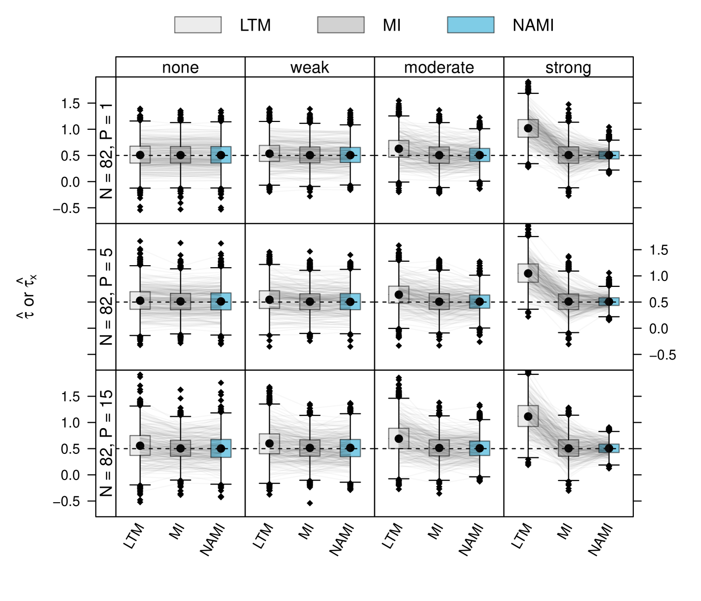
Figure 1: Empirical experiments for normally distributed outcome under $\tau=0.5$ (dashed lines): Distribution of treatment effect estimates $\hat{\tau}$ of Cohen’s $d$ obtained from unadjusted marginal inference (MI) and nonparanormal adjusted marginal inference (NAMI), and effect estimates of $\hat{\tau}_{\text{\boldmath$x$}}$ by linear transformation models (LTM) under varying prognostic strengths of covariate $X_{1}$ (in columns) and increasing number of noise covariates ($P$, in rows).

Table 1: Empirical experiments: Estimated power for different outcome types for Wald tests obtained from linear transformation models (LTM), unadjusted marginal inference (MI), and nonparanormal adjusted marginal inference (NAMI) under varying prognostic strength of covariate $X_{1}$ (in columns) and varying number of (noise) covariates ($P$, in rows). For binary and survival outcomes, results for the standardization approaches of Zhang et al. (2008) and Lu and Tsiatis (2008) (YSTD), and Ye et al. (2024) (LRCL) are also reported. For survival outcomes, results are only shown for heavy censoring.

			Power
DGP	Algorithm	P	none	weak	moderate	strong
normal	LTM	P = 1	0.611	0.663	0.784	0.994
		P = 5	0.622	0.645	0.782	0.994
		P = 15	0.604	0.650	0.767	0.988
	MI	P = 1	0.610	0.617	0.620	0.619
		P = 5	0.629	0.615	0.621	0.626
		P = 15	0.609	0.628	0.628	0.624
	NAMI	P = 1	0.613	0.669	0.802	0.999
		P = 5	0.620	0.648	0.801	0.999
		P = 15	0.604	0.653	0.776	0.998
binary	LTM	P = 1	0.589	0.611	0.698	0.937
		P = 5	0.599	0.620	0.707	0.933
		P = 15	0.601	0.621	0.703	0.920
	MI	P = 1	0.588	0.592	0.594	0.611
		P = 5	0.603	0.600	0.596	0.599
		P = 15	0.601	0.593	0.600	0.610
	NAMI	P = 1	0.587	0.617	0.711	0.940
		P = 5	0.600	0.625	0.717	0.940
		P = 15	0.602	0.624	0.714	0.930
	YSTD	P = 1	0.590	0.615	0.704	0.939
		P = 5	0.603	0.626	0.716	0.939
		P = 15	0.611	0.630	0.716	0.932
survival	LTM	P = 1	0.625	0.639	0.746	0.966
		P = 5	0.614	0.634	0.743	0.971
		P = 15	0.601	0.632	0.724	0.960
	MI	P = 1	0.626	0.607	0.614	0.601
		P = 5	0.619	0.608	0.614	0.623
		P = 15	0.605	0.605	0.618	0.612
	NAMI	P = 1	0.628	0.642	0.755	0.984
		P = 5	0.619	0.639	0.759	0.988
		P = 15	0.610	0.632	0.749	0.983
	LRCL	P = 1	0.620	0.621	0.678	0.775
		P = 5	0.619	0.625	0.690	0.782
		P = 15	0.621	0.638	0.702	0.790
	YSTD	P = 1	0.638	0.627	0.647	0.648
		P = 5	0.669	0.659	0.680	0.691
		P = 15	0.687	0.690	0.701	0.702

RQ 1: Unbiased estimation?

Overall, MI and NAMI produced nearly unbiased parameter estimates of the true marginal effect under all conditions (Figure 1 and Figure  S. 4, Appendix C for binary and survival outcomes). The corresponding boxplots of $\hat{\tau}$ were symmetrically distributed around $\tau$. In contrast, adjusting for covariates led to much larger values $\hat{\tau}_{\text{\boldmath$x$}}$ for LTM whenever the number of covariates was large or at least one of them weakly informative, illustrating the effect of noncollapsibility. The estimates were highly correlated in all scenarios. When adjusting for a single noninformative covariate $X_{1}$ (top-left panel), NAMI, MI and LTM performed on par. For binary and survival outcomes, competing methods YSTD and LRCL also obtained nearly unbiased marginal estimates.

RQ 2: Reduced standard errors?

The first columns in Figures  S. 2 and S. 5 show that the standard errors of NAMI were slightly larger compared to the standard errors obtained from MI when adjusting for one or more noninformative covariates. This reflected the increased variability of the NAMI parameter estimates visible in the first column of Figure 1 and Figure  S. 4. When adjusting for one moderate or strong prognostic covariate, smaller standard errors for NAMI corresponded to the decreased variability of the corresponding parameter estimates. Similar results were obtained for binary and survival outcomes. Distributions of standard errors were similar for YSTD and NAMI for binary outcomes; for survival outcomes, standard errors of NAMI were lower than for YSTD when $X_{1}$ was at least moderate prognostic. Table 1 shows that higher prognostic strength leads to higher power. YSTD and NAMI performed similar in this regard for binary outcomes, while power was higher for NAMI compared to YSTD and LRCL for survival outcomes.

RQ 3: Influence of prognostic strength?

Increasing the prognostic strength of $X_{1}$ led to less variable estimates $\hat{\tau}$ (first row in Figure 1 and Figure  S. 4), smaller standard errors (first row in Figures  S. 2 and S. 5), and higher power (Table 1) for NAMI in comparison to MI. For binary outcomes, YSTD performed similarly to NAMI, while for survival outcomes, NAMI had less variable estimates at higher prognostic levels, leading to smaller standard errors and larger power compared to YSTD and LRCL.

RQ 4: Sensitivity to noise variables?

Adding noise variables had surprisingly little influence on the performance of NAMI (first column of Figures  S. 2 and S. 5) and only induced bias for the LTM. However, there was an increase in the variability of the $\tau$ estimates obtained by NAMI and MI and their standard errors, especially for $P=15$ covariates. These patterns were also visible for binary and survival outcomes shown in Appendix C. YSTD and LRCL behaved similarly to NAMI in this respect (little influence, slightly increased variance). If $X_{1}$ was only weakly prognostic and $P=15$, NAMI did not always identify $X_{1}$ as the most prognostic covariate (Table  S. 2). This was particularly the case when the sample size was small in the continuous setting. In this case, no reliable inference by LTM and NAMI can be guaranteed, as the empirical sizes in Table  S. 1 exceeded the nominal size and the empirical distributions of the $p$-values in Figures  S. 6 and S. 3 deviated from the uniform distribution. Liberality of YSTD and LRCL under heavy censoring is shown in Table  S. 1.

Overall, these results suggest the potential of nonparanormal adjusted marginal inference to bypass the problems induced by noncollapsibility of effect measures such as Cohen’s $d$, log-odds ratios, or log-hazard ratios. The method combines unbiased parameter estimates of marginally defined parameters with covariate adjustment leading to reduced standard errors, and thus narrower Wald confidence intervals, compared to unadjusted marginal inference. At the same time, it avoids the bias induced by adding covariates to noncollapsible conditional models illustrated by the simulation results for the linear transformation model. The advantage over the marginal analysis became more pronounced as the prognostic strength increased. Adding noise variables had no large effect on the adjusted parameter estimates if the sample size was sufficiently large.

4 Applications

We present three applications of nonparanormal adjusted marginal inference for Cohen’s $d$ in an equivalence trial, for odds ratios in $2\times 2$ tables, and for hazard ratios in survival analysis.

Continuous outcome: Immunotoxicity study on Chloramine

Data on the effect of Chloramine-dosed water on the weight of female mice were reported as part of the National Toxicology Program. Repeated measurements were conducted on days $1$, $8$, $15$, $22$, and $29$ in five dose groups ($0$, $2$, $10$, $20$, $100$ mg/kg). We focus on the comparison of the highest dose ($W=1,N_{1}=40$) with the control group ($W=0,N_{0}=40$) with respect to outcome $Y$, the weight at day $29$. The weight on day $1$ is used as the only covariate $X_{1}$. We test the equivalence hypothesis “no effect of Chloramine on weight” formulated in terms of Cohen’s $d$ as the marginal treatment effect $\tau$. The two-sided alternative states that $\tau$ is in the equivalence interval $(-\delta,\delta)$ with corresponding $H_{0}:|\tau|\geq\delta$. We reject $H_{0}$ at $5\%$ when the $95\%$ confidence interval for Cohen’s $d$ is completely contained in the equivalence interval. Because Cohen’s $d$ does not depend on the measurement scale of the outcome, recommendations for $\delta$ exist (with $\delta=0.36$ we follow Table 1.1 given by Wellek, 2010, acknowledging this oversimplification in our choice of $\delta$). The unadjusted estimate of Cohen’s $d$ is $\hat{\tau}=0.048$. The standard errors computed from the observed Fisher information and the expected Fisher information (Lemma 1) evaluated at $\hat{\tau}$ are identical ($\text{SE}(\hat{\tau})=0.224$) and result in a $95\%$ Wald interval $(-0.390,0.486)$. The unadjusted analysis therefore does not lead to a rejection of $H_{0}$.

Adjusting for weight at baseline in nonparanormal adjusted marginal inference (with $h_{1}$ in Bernstein form), we obtain $\hat{\tau}=-0.002$ for the marginal Cohen’s $d$. The standard error obtained from the observed Fisher information and the theoretical standard error from Lemma 2 (evaluated at the maximum-likelihood estimates $\hat{\tau}$ and $\hat{\lambda}=-0.800$) both give $0.175$ and lead to the Wald interval $(-0.344,0.341)$. This interval is completely contained in the equivalence interval and thus the absence of an effect of Chloramine on weight can be inferred. The reduction in standard error comes from the high association between the outcome $Y$ and the covariate $X_{1}$ ($\rho(\hat{\lambda})=0.625$). The coefficient of determination was $R^{2}=0.512$, suggesting a substantial improvement of the conditional over the marginal model.

Binary outcome: Efficacy study on new combined chemotherapy

Rödel et al. (2012) analysed the pathological complete response in rectal cancer patients as an early endpoint comparing fluorouracil-based standard of care ($W=0$, $N_{0}=623$) with a combination therapy adding oxaliplatin ($W=1$, $N_{1}=613$). The binary outcome $Y$ was defined by the absence of viable tumour cells in the primary tumour and lymph nodes after surgery. Rödel et al. (2012) reported an odds ratio of $1.40$ with $95\%$ confidence interval $(1.02,1.92)$ based on a Cochran-Mantel-Haenszel $\chi^{2}$ test stratified for lymph node involvement (positive vs. negative) and clinical T category (1–3 vs. 4). For data from the completed trial, the unadjusted marginal log-odds ratio estimated by a binary logistic regression is $0.352$ with corresponding $95\%$ Wald interval $(0.036,0.668)$.

When adjusting for six potentially prognostic covariates (age, sex, ECOG performance status, distance to the anal verge of the tumour and the two stratum variables lymph node involvement and clinical T category), the marginal log-odds ratio changes to $0.338$ with $95\%$ Wald interval $(0.022,0.654)$. The corresponding odds ratio $1.402$ with Wald interval $(1.023,1.923)$ is very close to the initial results for two reasons: Information from the two stratum variables is included while none of the six variables carries strong prognostic information (with $\hat{\rho}_{J,\text{ECOG}}=-0.150$ denoting the largest association to the binary outcome). Adjusting for covariates did neither improve fit ($R^{2}=0.030$) nor precision, however, adding six variables carrying little information also did not increase the standard error.

Survival outcome: Longevity study of male fruit flies

Partridge and Farquhar (1981) assessed whether sexual activity affects the lifespan of male fruit flies. A total of $N=125$ flies were randomly divided into five groups of $25$: males forced to live alone, males assigned to live with one or eight receptive females, and males assigned to live with one or eight nonreceptive females. For the sake of simplicity, we focus on the analysis of the two groups with eight female flies added that were either all nonreceptive ($W=0$) or receptive ($W=1$). The primary outcome $Y$ was the survival time of male flies in days. The thorax length $X_{1}$ of the male flies was also measured – a covariate that is strongly associated with longevity.

The marginal Cox proportional hazards model for time to death, with baseline log-cumulative hazard function $h$ in Bernstein form of order six, defines the marginal treatment effect as log-hazard ratio $\tau$. For thorax length, $h_{1}$ was also parameterised in Bernstein form with order six. The joint distribution of both variables was expressed by a Gaussian copula.

The unadjusted marginal log-hazard ratio is $\hat{\tau}=2.157$ with $95\%$ Wald interval $(1.343,2.970)$. The hazard of dying in the sexually active group is around $\exp(\hat{\tau})=8.641$ times higher than for the nonactive group. The adjusted log-hazard ratio is $2.048$, with shorter $95\%$ Wald interval $(1.431,2.666)$. The coefficient of determination $R^{2}=0.671$ indicates that thorax length is highly prognostic.

5 Discussion

Paranormal adjusted marginal inference introduces covariate adjustment for the estimation of noncollapsible marginal treatment effect parameters, most importantly of standardised differences in means, odds ratios and hazard ratios. The resulting marginal treatment effect estimates are less variable than their unadjusted counterparts when relevant prognostic information is available in baseline covariates. The estimates can be compared between different studies, for example for meta analyses, in research syntheses, or in replication studies. The reduced standard errors might help to design smaller trials – the sample size reduction factors presented in Figure  S. 1, for example, demonstrate the potential of nonparanormal adjusted marginal inference to reduce the necessary sample size in equivalence studies. However, a high level of evidence regarding the strength of prognostic variables is necessary a priori.

The combination of marginal and copula model can be criticised in light of data. Classical model fit criteria can be applied to the marginal models, for example a plot of cloglog-transformed Kaplan-Meier curves for assessing parallelism when the treatment effect was defined as a log-hazard ratio. Conceptually, one could refrain from defining a scalar treatment effect in the marginal model by fitting two separate transformations, and thus distribution functions $F_{w}(y)=\Phi(wh(y\mid 1)+(1-w)h(y\mid 0))$, to the outcomes in both treatment groups (similar in spirit to Kennedy et al., 2023), maybe followed by an omnibus test based on a Smirnov statistic $\sup_{y\in\mathcal{Y}}\mid F_{1}(y)-F_{0}(y)\mid$. Additive transformation models provide an alternative way of estimating the novel partially linear conditional transformation models (9), (11), or (13) where lack of monotonicity of the covariate effects indicates a lack of fit in the Gaussian copula structure. Parameter estimation in nonparanormal adjusted marginal inference can be sensitive to model misspecification. Appendix D demonstrates this for a survival outcome where nonparanormal adjusted marginal inference depends on a misspecified marginal Cox proportional hazards model. Because nonparanormal adjusted marginal inference ensures that the treatment effect is collapsible, omitted variables do not affect the marginal effect. Also goodness of fit remains unaffected: If the Gaussian copula structure is appropriate given all covariates, it can be assumed to fit well for any subset of covariates.

We evaluated our method based on its parameter estimates and standard errors, and we assessed power and size. These experiments suggest that nonparanormal adjusted marginal inference performed either on par (in the binary setting) or outperformed established semiparametric adjusted marginal inference procedures. Although the latter procedures have been derived in theoretically general terms (Zhang et al., 2008), currently only implementations tailored to specific cases (log-odds and log-hazard ratios) are available. The reference implementation of nonparanormal adjusted marginal inference allows estimation of marginal treatment effects for general transformation models for continuous and discrete outcomes under several forms of censoring. Thus, nonparanormal adjusted marginal inference provides an interesting alternative to these standard methods discussed in Van Lancker et al. (2024a). With a reference software implementation being available in the tram add-on package to the R system for statistical computing, nonparanormal adjusted marginal inference awaits further scrutiny by practitioners.

6 Computational details

All computations were performed using R version 4.4.0 (R Core Team, 2024). A reference implementation of marginal and multivariate transformation models is available in the R add-on package tram (Hothorn et al., 2025). The semiparametric standardisation approach of Zhang et al. (2008) and Lu and Tsiatis (2008) for binary and survival outcomes (referred to as YSTD in Section 3) is implemented in the speff2trial package (Juraska et al., 2022). The approach of Ye et al. (2024) for survival outcomes (referred to as LRCL in Section 3 and Section D) is available in RobinCar (Bannick et al., 2024). The simulation study was run in parallel with the batchtools package (Lang and Bischl, 2023). The code to reproduce the results discussed in Section 3 can be found at https://gitlab.uzh.ch/susanne.dandl1/marginal_noncollapsibility. Performing nonparanormal adjusted marginal inference in R is relatively straightforward. The core of the analysis of fruit fly survival in Section 4 is

library("tram")
## marginal normal model feat. Cohen’s d; unadjusted marginal inference
confint(m0 <- Lm(y ˜ w, data = d))
#      2.5 %   97.5 %
# -0.3901557 0.486494
m1 <- BoxCox(x ˜ 1, data = d) ## marginal model for baseline weight
confint(mmlt(m0, m1, formula = ˜ 1, data = d)) ## adjusted marginal inference
#      2.5 %     97.5 % 
# -0.3442240  0.3407635 

The complete analyses presented in Section 4 are reproducible from within R via:

library("tram")
demo("NAMI", package = "tram")

This code also demonstrates appropriateness of marginal and copula model assumptions for the three datasets via additive transformation models (Tamási, 2025).

Acknowledgements

Financial support by Swiss National Science Foundation, grant number 200021_219384, is acknowledged.

Appendix A Derivation of standard errors

The following provides the proofs for Lemma 1 and Lemma 2 of Section 2.3.

A.1 Proof of Lemma 1

Consider a normally distributed outcome $Y\mid W=w\sim\operatorname{N}(-(\vartheta_{1}-\tau w)\vartheta_{2}^{-1},\vartheta_{2}^{-2})$ with binary treatment indicator $W\in\{0,1\}$, $W\sim B(1,0.5)$. Compared to the linear marginal model (8), we model $Y$ with a positive instead of a negative shift term without loss of generality

$$F(y\mid W=w)=\Phi\left(\vartheta_{1}+\vartheta_{2}y+\tau w\right).$$

In the following, we define $\text{\boldmath$a$}(Y)=(1,Y,w)^{\top}$, $\text{\boldmath$\vartheta$}=(\vartheta_{1},\vartheta_{2},\tau)^{\top}$ such that $\text{\boldmath$a$}(Y)^{\top}\text{\boldmath$\vartheta$}:=\vartheta_{1}+\vartheta_{2}Y+\tau w.$ The derivative of the basis function is $\text{\boldmath$a$}^{\prime}(Y)=(0,1,0)^{\top}$. Consequently, the log-likelihood contribution of a single observation $(Y,w)$ is

$$l(\text{\boldmath$\vartheta$}) = \log(\phi(\text{\boldmath$a$}(Y)^{\top}\text{\boldmath$\vartheta$})\cdot\text{\boldmath$a$}^{\prime}(Y)^{\top}\text{\boldmath$\vartheta$})$$

$$\propto -\frac{1}{2}(\text{\boldmath$a$}(Y)^{\top}\text{\boldmath$\vartheta$})^{2}+\log(\text{\boldmath$a$}^{\prime}(Y)^{\top}\text{\boldmath$\vartheta$}).$$

The score contribution for $\vartheta$ is

$$s(\text{\boldmath$\vartheta$})=\frac{\partial l(\text{\boldmath$\vartheta$})}{\partial\text{\boldmath$\vartheta$}}=-\text{\boldmath$a$}(Y)\text{\boldmath$a$}(Y)^{\top}\text{\boldmath$\vartheta$}+\frac{\text{\boldmath$a$}^{\prime}(Y)}{\text{\boldmath$a$}^{\prime}(Y)^{\top}\text{\boldmath$\vartheta$}}.$$

and the negative Hessian is

$$-\mathcal{H}=-\dfrac{\partial l^{2}(\text{\boldmath$\vartheta$})}{\partial\text{\boldmath$\vartheta$}\partial\text{\boldmath$\vartheta$}}=\text{\boldmath$a$}(Y)\text{\boldmath$a$}(Y)^{\top}+\frac{\text{\boldmath$a$}^{\prime}(Y)\text{\boldmath$a$}^{\prime}(Y)^{\top}}{(\text{\boldmath$a$}^{\prime}(Y)^{\top}\text{\boldmath$\vartheta$})^{2}}.$$

The expected Fisher information is defined as

$$\mathbb{I}(\text{\boldmath$\vartheta$}) = \mathbb{E}_{Y\mid W=w}(-\mathcal{H})=\mathbb{E}\left(\text{\boldmath$a$}(Y)\text{\boldmath$a$}(Y)^{\top}+\frac{\text{\boldmath$a$}^{\prime}(Y)\text{\boldmath$a$}^{\prime}(Y)^{\top}}{(\text{\boldmath$a$}^{\prime}(Y)^{\,\top}\text{\boldmath$\vartheta$})^{2}}\right)$$

$$= \begin{pmatrix}[1.5]1&-\frac{\vartheta_{1}+\tau w}{\vartheta_{2}}&w\\ -\frac{\vartheta_{1}+\tau w}{\vartheta_{2}}&\frac{1+(\vartheta_{1}+\tau w)^{2}}{\vartheta_{2}^{2}}&-w\frac{\vartheta_{1}+\tau w}{\vartheta_{2}}\\ w&-w\frac{\vartheta_{1}+\tau w}{\vartheta_{2}}&w^{2}\end{pmatrix}+\begin{pmatrix}0&0&0\\ 0&\vartheta_{2}^{-2}&0\\ 0&0&0\end{pmatrix}$$

$$= \begin{pmatrix}[1.5]1&-\frac{\vartheta_{1}+\tau w}{\vartheta_{2}}&w\\ -\frac{\vartheta_{1}+\tau w}{\vartheta_{2}}&\frac{1+(\vartheta_{1}+\tau w)^{2}}{\vartheta_{2}^{2}}+\frac{1}{\vartheta_{2}^{2}}&-w\frac{\vartheta_{1}+\tau w}{\vartheta_{2}}\\ w&-w\frac{\vartheta_{1}+\tau w}{\vartheta_{2}}&w^{2}\end{pmatrix},$$

Given a balanced dataset with $N$ observations, the expected Fisher information for the whole sample is then

$$\mathbf{I}_{N}(\text{\boldmath$\vartheta$}) = \frac{N}{2}\left(\mathbb{E}_{Y\mid W=1}(-\mathcal{H})+\mathbb{E}_{Y\mid W=0}(-\mathcal{H})\right)$$

$$= \frac{N}{2}\begin{pmatrix}[1.5]2&-\frac{2\vartheta_{1}+\tau}{\vartheta_{2}}&1\\ -\frac{2\vartheta_{1}+\tau}{\vartheta_{2}}&\frac{1}{\vartheta_{2}^{2}}(4+(\vartheta_{1}+\tau)^{2}+\vartheta_{1}^{2})&-\frac{\vartheta_{1}+\tau}{\vartheta_{2}}\\ 1&-\frac{\vartheta_{1}+\tau}{\vartheta_{2}}&1\end{pmatrix}.$$

The square root of the third diagonal element of $\mathbf{I}^{-1}_{N}(\text{\boldmath$\vartheta$})$ is equal to the standard error of $\tau$

$$\text{SE}(\tau)=\sqrt{\mathbf{I}^{-1}_{N}(\text{\boldmath$\vartheta$})_{[3,3]}}=\sqrt{\frac{2}{N}\left(\frac{\tau^{2}}{4}+2\right)}.$$

∎

A.2 Proof of Lemma 2

Consider a normally distributed outcome $Y\mid W=w\sim\operatorname{N}(-(\vartheta_{1}-\tau w)/\vartheta_{2},1/\vartheta_{2}^{2})$ with binary treatment indicator $W\in\{0,1\}$, $W\sim B(1,0.5)$, and a normally distributed covariate $X\sim\operatorname{N}(-\vartheta_{21}/\vartheta_{22},1/\vartheta_{22}^{2})$. As in Section A.1, we use a positive instead of a negative shift term in the marginal model for $Y$

$$F_{Y}(y\mid W=w)=\Phi\left(\vartheta_{11}+\vartheta_{12}y+\tau w\right).$$

The marginal model for $X$ is parameterised as

$$F_{X}(x)=\Phi\left(\vartheta_{21}+\vartheta_{22}y\right).$$

We define $\text{\boldmath$a$}_{1}(Y)=(1,Y,w)^{\top}$, $\text{\boldmath$\vartheta$}_{1}=(\vartheta_{11},\vartheta_{12},\tau)^{\top}$ and $\text{\boldmath$a$}_{2}(X)=(1,X)^{\top}$ with $\text{\boldmath$\vartheta$}_{2}=(\vartheta_{21},\vartheta_{22})^{\top}$ such that $h(Y\mid W=w)=\text{\boldmath$a$}_{1}(Y)^{\top}\text{\boldmath$\vartheta$}_{1}$ and $h_{2}(X)=\text{\boldmath$a$}_{2}(X)^{\top}\text{\boldmath$\vartheta$}_{2}$.

Compared to Section 2.2, we interchange the ordering of $Y$ in $X$, such that $j=1$ corresponds to $Y$ instead of $X$. With $\text{\boldmath$h$}(Y,X\mid W=w)=(h(Y\mid W=w),h_{2}(X))^{\top}$, we have $\text{\boldmath$h$}(Y,X\mid W=w)\sim\operatorname{N}_{2}(\mathbf{0},\mathbf{\Lambda}^{-1}\mathbf{\Lambda}^{-\top}).$

The parametrisation of

$$\mathbf{\Sigma}=\mathbf{\Lambda}^{-1}\mathbf{\Lambda}^{-\top}=\begin{pmatrix}[1]1&-\lambda\\ -\lambda&1+\lambda^{2}\end{pmatrix}$$

slightly differs to the one used in Section 2.2 but leads to the same log-likelihood and inference for $\text{\boldmath$\vartheta$}_{1}$ (Hothorn, 2024).

Because $f_{Y,X}(y,x)=f_{Y}(y)\cdot f_{X\mid Y}(x\mid y)$, we can define the log-likelihood contribution based on the product of the densities

$$f_{Y}(y) = \phi(\text{\boldmath$a$}_{1}(y)^{\top}\text{\boldmath$\vartheta$}_{1})\cdot\text{\boldmath$a$}_{1}^{\prime}(y)^{\top}\text{\boldmath$\vartheta$}_{1}$$

$$f_{X\mid Y}(x\mid y) = \phi(\lambda\text{\boldmath$a$}_{1}(y)^{\top}\text{\boldmath$\vartheta$}_{1}+\text{\boldmath$a$}_{2}(x)^{\top}\text{\boldmath$\vartheta$}_{2})\cdot\text{\boldmath$a$}_{2}^{\prime}(x)^{\top}\text{\boldmath$\vartheta$}_{2}$$

The log-likelihood contribution for a single observation as a function of the parameters $\Theta=(\text{\boldmath$\vartheta$}_{1}^{\top},\text{\boldmath$\vartheta$}_{2}^{\top},\lambda)^{\top}$ is given by

$$\ell(\Theta) = \ell_{1}(\text{\boldmath$\vartheta$}_{1})+\ell_{2\mid 1}(\text{\boldmath$\vartheta$}_{1},\text{\boldmath$\vartheta$}_{2},\lambda)$$

$$= -\frac{1}{2}(\text{\boldmath$a$}_{1}(Y)^{\top}\text{\boldmath$\vartheta$}_{1})^{2}+\log(\text{\boldmath$a$}^{\prime}_{1}(Y)^{\top}\text{\boldmath$\vartheta$}_{1})$$

$$-\frac{1}{2}(\lambda\text{\boldmath$a$}_{1}(Y)^{\top}\text{\boldmath$\vartheta$}_{1}+\text{\boldmath$a$}_{2}(X)^{\top}\text{\boldmath$\vartheta$}_{2})^{2}+\log(\text{\boldmath$a$}^{\prime}_{2}(X)^{\top}\text{\boldmath$\vartheta$}_{2})$$

The corresponding score contributions are

$$s(\text{\boldmath$\vartheta$}_{1}) = \frac{\partial l(\Theta)}{\partial\text{\boldmath$\vartheta$}_{1}}=-\text{\boldmath$a$}_{1}(Y)\text{\boldmath$a$}_{1}(Y)^{\top}\text{\boldmath$\vartheta$}_{1}+\frac{\text{\boldmath$a$}^{\prime}_{1}(Y)}{\text{\boldmath$a$}^{\prime}_{1}(Y)^{\,\top}\text{\boldmath$\vartheta$}_{1}}-(\lambda\text{\boldmath$a$}_{1}(Y)^{\top}\text{\boldmath$\vartheta$}_{1}+\text{\boldmath$a$}_{2}(X)^{\top}\text{\boldmath$\vartheta$}_{2})\text{\boldmath$a$}_{1}(Y)\lambda$$

$$= -\text{\boldmath$a$}_{1}(Y)\text{\boldmath$a$}_{1}(Y)^{\top}\text{\boldmath$\vartheta$}_{1}+\frac{\text{\boldmath$a$}^{\prime}_{1}}{\text{\boldmath$a$}^{\prime}_{1}(Y)^{\,\top}\text{\boldmath$\vartheta$}_{1}}-\lambda^{2}\text{\boldmath$a$}_{1}(Y)^{\top}\text{\boldmath$\vartheta$}_{1}\text{\boldmath$a$}_{1}(Y)-\text{\boldmath$a$}_{2}(X)^{\top}\text{\boldmath$\vartheta$}_{2}\text{\boldmath$a$}_{1}(Y)\lambda$$

$$s(\text{\boldmath$\vartheta$}_{2}) = \frac{\partial l(\Theta)}{\partial\text{\boldmath$\vartheta$}_{2}}=-(\lambda\text{\boldmath$a$}_{1}(Y)^{\top}\text{\boldmath$\vartheta$}_{1}+\text{\boldmath$a$}_{2}(X)^{\top}\text{\boldmath$\vartheta$}_{2})\text{\boldmath$a$}_{2}(X)+\frac{\text{\boldmath$a$}^{\prime}_{2}(X)}{\text{\boldmath$a$}^{\prime}_{2}(X)^{\,\top}\text{\boldmath$\vartheta$}_{2}}$$

$$= -\lambda\text{\boldmath$a$}_{1}(Y)^{\top}\text{\boldmath$\vartheta$}_{1}\text{\boldmath$a$}_{2}(X)-\text{\boldmath$a$}_{2}(X)^{\top}\text{\boldmath$\vartheta$}_{2}\text{\boldmath$a$}_{2}(X)+\frac{\text{\boldmath$a$}^{\prime}_{2}(X)}{\text{\boldmath$a$}^{\prime}_{2}(X)^{\top}\text{\boldmath$\vartheta$}_{2}}$$

$$s(\lambda) = \frac{\partial l(\Theta)}{\partial\lambda}=-(\lambda\text{\boldmath$a$}_{1}(Y)^{\top}\text{\boldmath$\vartheta$}_{1}+\text{\boldmath$a$}_{2}(X)^{\top}\text{\boldmath$\vartheta$}_{2})\text{\boldmath$a$}_{1}(Y)^{\top}\text{\boldmath$\vartheta$}_{1}$$

$$= -\lambda(\text{\boldmath$a$}_{1}(Y)^{\top}\text{\boldmath$\vartheta$}_{1})^{2}-\text{\boldmath$a$}_{2}(X)^{\top}\text{\boldmath$\vartheta$}_{2}\text{\boldmath$a$}_{1}(Y)^{\top}\text{\boldmath$\vartheta$}_{1}$$

The negative Hessian is

$$-\mathcal{H} = \begin{pmatrix}[2]-\dfrac{\partial^{2}l(\Theta)}{\partial\text{\boldmath$\vartheta$}_{1}\partial\text{\boldmath$\vartheta$}_{1}}&-\dfrac{\partial^{2}l(\Theta)}{\partial\text{\boldmath$\vartheta$}_{1}\partial\text{\boldmath$\vartheta$}_{2}}&-\dfrac{\partial^{2}l(\Theta)}{\partial\text{\boldmath$\vartheta$}_{1}\partial\lambda}\\ -\dfrac{\partial^{2}l(\Theta)}{\partial\text{\boldmath$\vartheta$}_{2}\partial\text{\boldmath$\vartheta$}_{1}}&-\dfrac{\partial^{2}l(\Theta)}{\partial\text{\boldmath$\vartheta$}_{2}\partial\text{\boldmath$\vartheta$}_{2}}&-\dfrac{\partial^{2}l(\Theta)}{\partial\text{\boldmath$\vartheta$}_{2}\partial\lambda}\\ -\dfrac{\partial^{2}l(\Theta)}{\partial\lambda\partial\text{\boldmath$\vartheta$}_{1}}&-\dfrac{\partial^{2}l(\Theta)}{\partial\lambda\partial\text{\boldmath$\vartheta$}_{2}}&-\dfrac{\partial^{2}l(\Theta)}{\partial\lambda\partial\lambda}\end{pmatrix}$$ (14)

$$=\begin{pmatrix}[1]\text{\boldmath$a$}_{1}(Y)\text{\boldmath$a$}_{1}(Y)^{\top}+\frac{\text{\boldmath$a$}^{\prime}_{1}(Y)\text{\boldmath$a$}^{\prime}_{1}(Y)^{\top}}{(\text{\boldmath$a$}^{\prime}(Y)^{\top}_{1}\text{\boldmath$\vartheta$}_{1})^{2}}+\lambda^{2}\text{\boldmath$a$}_{1}(Y)\text{\boldmath$a$}_{1}(Y)^{\top}&\lambda\text{\boldmath$a$}_{1}(Y)\text{\boldmath$a$}_{2}(X)^{\top}&\left(2\lambda\text{\boldmath$a$}_{1}(Y)^{\top}\text{\boldmath$\vartheta$}_{1}+\text{\boldmath$a$}_{2}(X)^{\top}\text{\boldmath$\vartheta$}_{2}\right)\text{\boldmath$a$}_{1}(Y)\\ \lambda\text{\boldmath$a$}_{2}(X)\text{\boldmath$a$}_{1}(Y)^{\top}&\text{\boldmath$a$}_{2}(X)\text{\boldmath$a$}_{2}(X)^{\top}+\frac{\text{\boldmath$a$}^{\prime}_{2}(X)\text{\boldmath$a$}^{\prime}_{2}(X)^{\top}}{(\text{\boldmath$a$}_{2}^{\prime}(X)^{\top}\text{\boldmath$\vartheta$}_{2})^{2}}&\text{\boldmath$a$}_{1}(Y)^{\top}\text{\boldmath$\vartheta$}_{1}\text{\boldmath$a$}_{2}(X)\\ \left(2\lambda\text{\boldmath$a$}_{1}(Y)^{\top}\text{\boldmath$\vartheta$}_{1}+\text{\boldmath$a$}_{2}(X)^{\top}\text{\boldmath$\vartheta$}_{2}\right)\text{\boldmath$a$}_{1}(Y)^{\top}&\text{\boldmath$a$}_{1}(Y)^{\top}\text{\boldmath$\vartheta$}_{1}\text{\boldmath$a$}_{2}(X)^{\top}&(\text{\boldmath$a$}_{1}(Y)^{\top}\text{\boldmath$\vartheta$}_{1})^{2}\end{pmatrix}$$

We are interested in the expected Fisher information $\mathbb{I}(\Theta)=\mathbb{E}_{(Y,X)\mid W=w}(-\mathcal{H})$ with $\mathcal{H}$ from Equation (14) with block entries

$$\mathbb{E}\left(\text{\boldmath$a$}_{1}(Y)\text{\boldmath$a$}_{1}(Y)^{\top}+\frac{\text{\boldmath$a$}^{\prime}_{1}(Y)\text{\boldmath$a$}^{\prime}_{1}(Y)^{\top}}{(\text{\boldmath$a$}^{\prime}_{1}(Y)^{\top}\text{\boldmath$\vartheta$}_{1})^{2}}+\lambda^{2}\text{\boldmath$a$}_{1}(Y)\text{\boldmath$a$}_{1}(Y)^{\top}\right)$$

$$\quad=(1+\lambda^{2})\begin{pmatrix}[1.5]1&-\frac{\vartheta_{11}+\tau w}{\vartheta_{12}}&w\\ -\frac{\vartheta_{11}+\tau w}{\vartheta_{12}}&\frac{1+(\vartheta_{11}+\tau w)^{2}}{\vartheta_{12}^{2}}&-w\frac{\vartheta_{11}+\tau w}{\vartheta_{12}}\\ w&-w\frac{\vartheta_{11}+\tau w}{\vartheta_{12}}&w^{2}\end{pmatrix}+\begin{pmatrix}0&0&0\\ 0&\vartheta_{12}^{-2}&0\\ 0&0&0\end{pmatrix}$$

$$\quad=\begin{pmatrix}[1.5]1+\lambda^{2}&-(1+\lambda^{2})\frac{\vartheta_{11}+\tau w}{\vartheta_{12}}&(1+\lambda^{2})w\\ -(1+\lambda^{2})\frac{\vartheta_{11}+\tau w}{\vartheta_{12}}&(1+\lambda^{2})\frac{1+(\vartheta_{11}+\tau w)^{2}}{\vartheta_{12}^{2}}+\frac{1}{\vartheta_{12}^{2}}&-(1+\lambda^{2})w\frac{\vartheta_{11}+\tau w}{\vartheta_{12}}\\ (1+\lambda^{2})w&-(1+\lambda^{2})w\frac{\vartheta_{11}+\tau w}{\vartheta_{12}}&(1+\lambda^{2})w^{2}\end{pmatrix},$$

$$\mathbb{E}\left(\text{\boldmath$a$}_{2}(X)\text{\boldmath$a$}_{2}(X)^{\top}+\frac{\text{\boldmath$a$}^{\prime}_{2}(X)\text{\boldmath$a$}^{\prime}_{2}(X)^{\top}}{(\text{\boldmath$a$}^{\prime}_{2}(X)^{\top}\text{\boldmath$\vartheta$}_{2})^{2}}\right)=\begin{pmatrix}[1.5]1&-\frac{\vartheta_{21}}{\vartheta_{22}}\\ -\frac{\vartheta_{21}}{\vartheta_{22}}&\frac{2+\lambda^{2}+\vartheta_{21}^{2}}{\vartheta_{22}^{2}}\end{pmatrix},$$

$$\mathbb{E}(\lambda\text{\boldmath$a$}_{1}(Y)\text{\boldmath$a$}_{2}(X)^{\top})=\begin{pmatrix}[1.5]\lambda&-\lambda\frac{\vartheta_{21}}{\vartheta_{22}}\\ -\lambda\frac{(\vartheta_{11}+\tau w)}{\vartheta_{12}}&\frac{\lambda(\vartheta_{11}+\tau w)\vartheta_{21}-\lambda^{2}}{\vartheta_{12}\vartheta_{22}}\\ \lambda w&-\lambda w\frac{\vartheta_{21}}{\vartheta_{22}}\end{pmatrix},$$

$$\mathbb{E}\left(2\lambda\text{\boldmath$a$}_{1}(Y)^{\top}\text{\boldmath$\vartheta$}_{1}\text{\boldmath$a$}_{1}(Y)+\text{\boldmath$a$}_{2}(X)^{\top}\text{\boldmath$\vartheta$}_{2}\text{\boldmath$a$}_{1}(Y)\right)$$

$$\quad=\mathbb{E}\left(\text{\boldmath$a$}_{1}(Y)\left(2\lambda\text{\boldmath$a$}_{1}(Y)^{\top}\text{\boldmath$\vartheta$}_{1}+\text{\boldmath$a$}_{2}(X)^{\top}\text{\boldmath$\vartheta$}_{2}\right)\right)$$

$$\quad=\mathbb{E}\left(\begin{pmatrix}[1]1\\ Y\\ w\end{pmatrix}\left(2\lambda\text{\boldmath$a$}_{1}(Y)^{\top}\text{\boldmath$\vartheta$}_{1}+\text{\boldmath$a$}_{2}(X)^{\top}\text{\boldmath$\vartheta$}_{2}\right)\right)$$

$$\quad\underset{\mathbb{E}(\text{\boldmath$a$}_{2}(X)^{\top}\text{\boldmath$\vartheta$}_{2})=0}{\overset{\mathbb{E}(\text{\boldmath$a$}_{1}(Y)^{\top}\text{\boldmath$\vartheta$}_{1})=0}{=}}\begin{pmatrix}[1]0\\ \mathbb{E}\left(Y\left(2\lambda\text{\boldmath$a$}_{1}(Y)^{\top}\text{\boldmath$\vartheta$}_{1}+\text{\boldmath$a$}_{2}(X)^{\top}\text{\boldmath$\vartheta$}_{2}\right)\right)\\ 0\end{pmatrix}=\begin{pmatrix}[1]0\\ \lambda\vartheta_{12}^{-1}\\ 0\end{pmatrix},$$

$$\mathbb{E}(\text{\boldmath$a$}_{1}(Y)^{\top}\text{\boldmath$\vartheta$}_{1}\text{\boldmath$a$}_{2}(X))=\mathbb{E}\left((\vartheta_{11}+\vartheta_{12}Y+\tau w)\begin{pmatrix}[1]1\\ X\end{pmatrix}\right)=\begin{pmatrix}[1]0\\ -\lambda\vartheta_{22}^{-1}\end{pmatrix},\text{ and}$$

$$\mathbb{E}(\text{\boldmath$a$}_{1}(Y)^{\top}\text{\boldmath$\vartheta$}_{1})^{2})=1.$$

Taken together, the expected Fisher information $\mathbb{I}(\Theta)$ of a single observation is

$$\tiny\begin{pmatrix}[1.5]1+\lambda^{2}&-(1+\lambda^{2})\frac{\vartheta_{11}+\tau w}{\vartheta_{12}}&(1+\lambda^{2})w&\lambda&-\lambda\frac{\vartheta_{21}}{\vartheta_{22}}&0\\ -(1+\lambda^{2})\frac{\vartheta_{11}+\tau w}{\vartheta_{12}}&(1+\lambda^{2})\frac{1+(\vartheta_{11}+\tau w)^{2}}{\vartheta_{12}^{2}}+\frac{1}{\vartheta_{12}^{2}}&-(1+\lambda^{2})w\frac{\vartheta_{11}+\tau w}{\vartheta_{12}}&-\lambda\frac{(\vartheta_{11}+\tau w)}{\vartheta_{12}}&\frac{\lambda(\vartheta_{11}+\tau w)\vartheta_{21}-\lambda^{2}}{\vartheta_{12}\vartheta_{22}}&\frac{\lambda}{\vartheta_{12}}\\ (1+\lambda^{2})w&-(1+\lambda^{2})w\frac{\vartheta_{11}+\tau w}{\vartheta_{12}}&(1+\lambda^{2})w^{2}&\lambda w&-\lambda w\frac{\vartheta_{21}}{\vartheta_{22}}&0\\ \lambda&-\lambda\frac{(\vartheta_{11}+\tau w)}{\vartheta_{12}}&\lambda w&1&-\frac{\vartheta_{21}}{\vartheta_{22}}&0\\ -\lambda\frac{\vartheta_{21}}{\vartheta_{22}}&\frac{\lambda(\vartheta_{11}+\tau w)\vartheta_{21}-\lambda^{2}}{\vartheta_{12}\vartheta_{22}}&-\lambda w\frac{\vartheta_{21}}{\vartheta_{22}}&-\frac{\vartheta_{21}}{\vartheta_{22}}&\frac{2+\lambda^{2}+\vartheta_{21}^{2}}{\vartheta_{22}^{2}}&-\frac{\lambda}{\vartheta_{22}}\\ 0&\frac{\lambda}{\vartheta_{12}}&0&0&-\frac{\lambda}{\vartheta_{22}}&1\end{pmatrix}.$$

Given a balanced dataset with $N$ observations, the expected Fisher information for the whole sample

$$\mathbf{I}_{N}(\Theta)=\frac{N}{2}\left(\mathbb{E}_{Y,X\mid W=1}(-\mathcal{H})+\mathbb{E}_{Y,X\mid W=0}(-\mathcal{H})\right)$$

is given by the matrix

$$\frac{N}{2}\begin{pmatrix}[1.5]2(1+\lambda^{2})&-(1+\lambda^{2})\frac{2\vartheta_{11}+\tau}{\vartheta_{12}}&(1+\lambda^{2})&2&-\frac{2\vartheta_{21}}{\vartheta_{22}}&0\\ -(1+\lambda^{2})\frac{2\vartheta_{11}+\tau}{\vartheta_{12}}&(1+\lambda^{2})\frac{1}{\vartheta_{12}^{2}}(4+(\vartheta_{11}+\tau)^{2}+\vartheta_{11}^{2})&-(1+\lambda^{2})\frac{\vartheta_{11}+\tau}{\vartheta_{12}}&-\frac{(2\vartheta_{11}+\tau)}{\vartheta_{12}}&\frac{(2\vartheta_{11}+\tau)\vartheta_{21}-2\lambda}{\vartheta_{12}\vartheta_{22}}&\frac{2}{\vartheta_{12}}\\ (1+\lambda^{2})&-(1+\lambda^{2})\frac{\vartheta_{11}+\tau}{\vartheta_{12}}&(1+\lambda^{2})&1&-\frac{\vartheta_{21}}{\vartheta_{22}}&0\\ 2&-\frac{(2\vartheta_{11}+\tau)}{\vartheta_{12}}&1&2&-2\frac{\vartheta_{21}}{\vartheta_{22}}&0\\ -\frac{2\vartheta_{21}}{\vartheta_{22}}&\frac{(2\vartheta_{11}+\tau)\vartheta_{21}-2\lambda}{\vartheta_{12}\vartheta_{22}}&-\frac{\vartheta_{21}}{\vartheta_{22}}&-\frac{\vartheta_{21}}{\vartheta_{22}}&\frac{2+\lambda^{2}+\vartheta_{21}^{2}}{\vartheta_{22}^{2}}&-\frac{\lambda}{\vartheta_{22}}\\ 0&\frac{2}{\vartheta_{12}}&0&0&-\frac{\lambda}{\vartheta_{22}}&1\end{pmatrix}$$

whose inverse $\mathbf{I}^{-1}_{N}(\Theta)$ is given by

$$\frac{2}{N}\begin{pmatrix}\frac{\lambda^{4}+\vartheta_{11}^{2}\,\lambda^{2}+\vartheta_{11}^{2}+4\,\lambda^{2}+4}{2\,\lambda^{4}+6\,\lambda^{2}+4}&{{{\vartheta_{11}\,\vartheta_{12}}\over{2\,\lambda^{2}+4}}}&{{{\vartheta_{11}\,\tau\,\lambda^{2}}}+{{\vartheta_{11}\,\tau}}-{{2\lambda^{2}}}-{{4}}}\over{2\,\lambda^{4}+6\,\lambda^{2}+4}&-{{\lambda}\over{2}}&0&-{{\vartheta_{11}\,\lambda}\over{2\,\lambda^{2}+4}}\\ {{\vartheta_{11}\,\vartheta_{12}}\over{2\,\lambda^{2}+4}}&{{\vartheta_{12}^{2}}\over{2\,\lambda^{2}+4}}&{{\vartheta_{12}\,\tau}\over{2\,\lambda^{2}+4}}&0&0&-{{\vartheta_{12}\,\lambda}\over{2\,\lambda^{2}+4}}\\ {{\vartheta_{11}\,\tau\,\lambda^{2}}+{{\vartheta_{11}\,\tau}}-{{2\lambda^{2}}}-{{4}}}\over{2\,\lambda^{4}+6\,\lambda^{2}+4}&{{\vartheta_{12}\,\tau}\over{2\,\lambda^{2}+4}}&{{(1+\lambda^{2})\tau^{2}+(2+\lambda^{2})4}\over{2\,\lambda^{4}+6\,\lambda^{2}+4}}&0&0&-{{\tau\,\lambda}\over{2\,\lambda^{2}+4}}\\ -{{\lambda}\over{2}}&0&0&{{\lambda^{2}}\over{2}}+{{\vartheta_{21}^{2}}\over{4}}+{{1}\over{2}}&{{\vartheta_{21}\,\vartheta_{22}}\over{4}}&{{\vartheta_{21}\,\lambda}\over{4}}\\ 0&0&0&{{\vartheta_{21}\,\vartheta_{22}}\over{4}}&{{\vartheta_{22}^{2}}\over{4}}&{{\vartheta_{22}\,\lambda}\over{4}}\\ -{{\vartheta_{11}\,\lambda}\over{2\,\lambda^{2}+4}}&-{{\vartheta_{12}\,\lambda}\over{2\,\lambda^{2}+4}}&-{{\tau\,\lambda}\over{2\,\lambda^{2}+4}}&{{\vartheta_{21}\,\lambda}\over{4}}&{{\vartheta_{22}\,\lambda}\over{4}}&{{\lambda^{4}}\over{4\,\lambda^{2}+8}}+{{3\,\lambda^{2}}\over{2\,\lambda^{2}+4}}+{{1}\over{\lambda^{2}+2}}\end{pmatrix}.$$

The square root of the third diagonal element of $\mathbf{I}^{-1}_{N}(\Theta)$ is equal to the standard error of $\tau$

$$\text{SE}(\tau,\lambda)=\sqrt{\mathbf{I}^{-1}_{N}(\Theta)_{[3,3]}}={\sqrt{\frac{2}{N}\left({(1+\lambda^{2})\tau^{2}+(2+\lambda^{2})4}\over{2\,\lambda^{4}+6\,\lambda^{2}+4}\right)}}.$$

∎

Figure S. 1: Theoretical fraction $\nicefrac{{\text{SE}(\tau,\lambda)^{2}}}{{\text{SE}(\tau)^{2}}}$ of the adjusted and unadjusted squared standard errors for Cohen’s $d$ (the treatment effect $\tau$) in a normal model with one prognostic variable whose correlation to the outcome is given by $\rho=-\nicefrac{{\lambda}}{{\sqrt{1+\lambda^{2}}}}$. The numbers can be interpreted as the fraction of the sample size required in a trial adjusting for prognostic information relative to the sample size required for a trial without such an adjustment.

Appendix B Sample size calculation

We derived the sample size for unadjusted marginal tests against null hypothesis $H_{0}:\tau=0$ vs. $H_{1}:\tau\neq 0$ for continuous (normally distributed), binary (binomially distributed) and survival (Weibull distributed) outcomes with true treatment effect $\tau=0.5$, size $\alpha=0.05$ and power $1-\beta=0.6$.

B.1 Continuous outcome

For continuous outcomes, the sample size calculation for each treatment group was based on

$$N_{1,\text{cont}}=N_{0,\text{cont}}=\left(\frac{\text{SE}(\tau)\left(z_{\beta}-z_{1-\tfrac{\alpha}{2}}\right)}{\tau}\right)^{2}=\left(\frac{\text{SE}(0.5)\left(z_{0.4}-z_{0.975}\right)}{0.5}\right)^{2}=41$$

for each control/treatment group. The derivation is based on maximum likelihood theory, according to which the distribution of the maximum likelihood estimator $\hat{\tau}$ is normally distributed with

$$\sqrt{N}\frac{\hat{\tau}}{\text{SE}(\tau)}\sim\operatorname{N}\left(\frac{\tau}{\text{SE}(\tau)},\frac{1}{N}\right).$$

Since we aim for equally sized treatment/control groups, it is suitable to derive $N_{1}=N_{0}$ for a single group by obtaining the value via the one-sided null hypothesis $H_{0}:\tau\leq 0$ vs. $H_{1}:\tau>0$:

$$1-\beta = 1-\mathbb{P}\left(\frac{\hat{\tau}}{\text{SE}(\tau)}\leq\frac{z_{1-\frac{\alpha}{2}}}{\sqrt{N_{1}}}\right)$$

$$\beta = \mathbb{P}\left(\frac{\hat{\tau}}{\text{SE}(\tau)}\leq\frac{z_{1-\frac{\alpha}{2}}}{\sqrt{N_{1}}}\right)$$

$$\beta = \Phi\left(\sqrt{N_{1}}\left(\frac{z_{1-\frac{\alpha}{2}}}{\sqrt{N_{1}}}-\frac{\tau}{\text{SE}(\tau)}\right)\right)$$

$$\Phi^{-1}(\beta)-z_{1-\frac{\alpha}{2}} = -\sqrt{N_{1}}\frac{\tau}{\text{SE}(\tau)}$$

$$N_{1} = \left(\frac{\text{SE}(\tau)\left(\Phi^{-1}\left(\beta\right)-z_{1-\frac{\alpha}{2}}\right)}{\tau}\right)^{2}.$$

The formula to compute the standard error for the setting without covariate adjustment $\text{SE}(\tau)$ is given in Lemma 1.

B.2 Binary outcome

For binary outcomes, the sample calculation was based on Formula (4.14) in Fleiss et al. (2003)

$$N_{1,\text{binary}}=\frac{\left(z_{\frac{\alpha}{2}}\sqrt{(p_{1}+p_{2})\left(1-\frac{p_{1}+p_{2}}{r+1}\right)}+z_{\beta}\sqrt{rp_{1}(1-p_{1})+p_{2}(1-p_{2})}\right)^{2}}{r(p_{1}-p_{2})^{2}},$$

where $r$ is the proportion of treated to control patients (here, $1$), $p_{1}=\tfrac{p_{2}\exp(\tau)}{(1+p_{2}(\exp(\tau)-1))}$ with $p_{2}$ as the proportion of controls with outcome $Y=1$. A value of $p_{2}=0.5$ was obtained based on a small experiment with 100 observations, sampled from the above described data generating process for binary data. With $\tau=0.5$, $1-\beta=0.6$ and $\alpha=0.05$, we obtained a sample size of $N_{1,\text{binary}}=161$ for each control/treatment group.

B.3 Survival outcome

The sample size calculation for survival outcomes was based on Formula (3) in Wu (2015)

$$N_{1,\text{surv}}=\frac{(r+1)^{2}}{r}\frac{(z_{1-\frac{\alpha}{2}}+z_{1-\beta})^{2}}{\tau^{2}(p_{0}+rp_{1})},$$

where $r$ is the proportion of treated to control patient (here, $1$), $p_{0}$ is the noncensoring probability for a control observation and $p_{1}$ is the noncensoring probability for a treated observation. For a noncensoring probability of 0.3 – a worst case scenario we indeed considered for the survival outcome – we obtained a sample size of $N_{1,\text{surv}}=131$ for each group (given $\tau=0.5$, $1-\beta=0.6$ and $\alpha=0.05$).

Appendix C Simulation study

C.1 Details on the Study Setup

For the Weibull distributed $Y$, we additionally added right-censoring by sampling censoring times $C$ from the conditional distribution function $\mathbb{P}(C\leq c\mid W=w,\text{\boldmath$X$}=\text{\boldmath$x$})=\Phi\left(\omega_{21}h_{1}(x_{1})+\omega_{22}\Phi^{-1}\left(\text{cloglog}^{-1}(\vartheta_{1}+\vartheta_{2}\log(c)-\gamma-\tau w)\right)\right)$ with $\vartheta_{1}=0$ and $\vartheta_{2}=1$. An observation was not censored if $Y<C$. The parameter $\gamma$ defines the probabilistic index, that is, the noncensoring probability $P(T<C\mid W=W,\text{\boldmath$X$}=\text{\boldmath$x$})=\text{logit}^{-1}(\gamma)$ (see Table 1 in Sewak and Hothorn, 2023). In our experiments, we employed values of $\gamma$ corresponding to noncensoring probabilities of $0.3$ (heavy censoring), $0.5$ (mild censoring) and $0.7$ (low censoring).

NAMI and MI relied on the following, correctly specified, marginal models for $Y$: The linear model (8) was used for the continuous (normally distributed) outcome; a logistic regression model (10) for the binary outcome; and a Cox proportional hazards model for survival outcomes (i.e., model (12) with $h(y)$ parameterised by a polynomial in Bernstein form of order six). For NAMI, the marginal distribution functions $\Phi(h_{j}(x_{j}))$ of the $P=J-1$ covariates were parameterised by a polynomial in Bernstein form of order six.

For NAMI, the marginal distribution functions $\Phi(h_{j}(x_{j}))$ of the $P=J-1$ covariates were parameterised by a polynomial in Bernstein form of order six. Thus, NAMI always relied on the misspecified marginal model for $X_{1}$ and was overparameterised in the presence of noise variables. Because only one out of $P=J-1$ covariates was potentially prognostic, only one out of $\nicefrac{{J(J-1)}}{{2}}$ parameters in $\lambda$ was potentially nonzero. The LTM was overparameterised in the setup with nonprognostic covariate $X_{1}$ (that is, with $\text{\boldmath$\beta$}=\mathbf{0}$) and misspecified in all other setups.

C.2 Continuous outcome

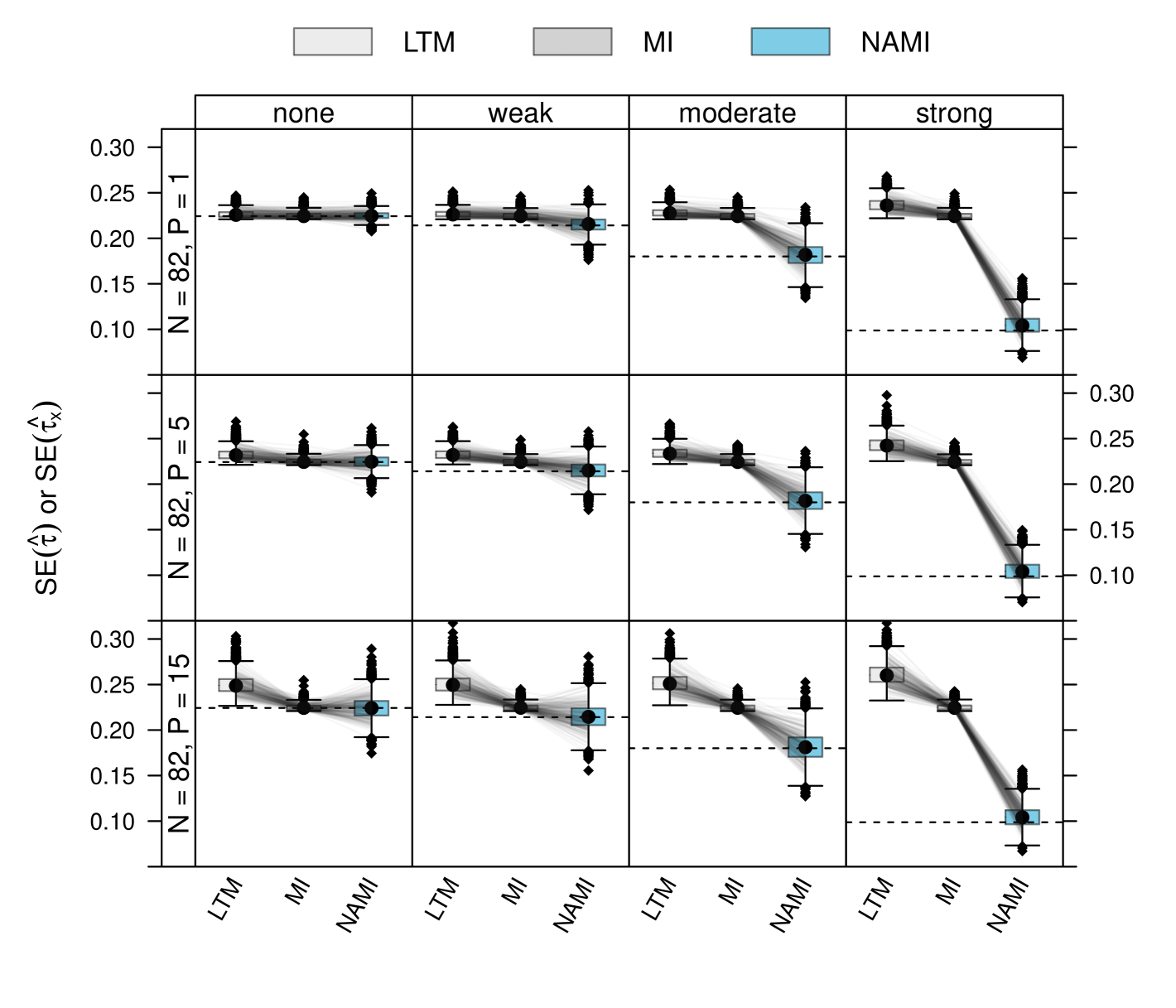
Figure S. 2: Empirical experiments for normally distributed outcome under $\tau=0.5$: Distribution of standard errors of treatment effect estimates $\hat{\tau}$ of Cohen’s $d$ obtained from unadjusted marginal inference (MI) and nonparanormal adjusted marginal inference (NAMI), and effect estimates of $\hat{\tau}_{\text{\boldmath$x$}}$ by linear transformation models (LTM) under varying prognostic strengths of covariate $X_{1}$ (in columns) and increasing number of noise covariates ($P$, in rows). Standard errors were computed by inverting the numerically determined negative Hessian. The dashed lines correspond to the theoretical standard errors $\text{SE}(\tau,\lambda)$ given true $\tau=0$ and differing true $\lambda$ (Lemma 2).

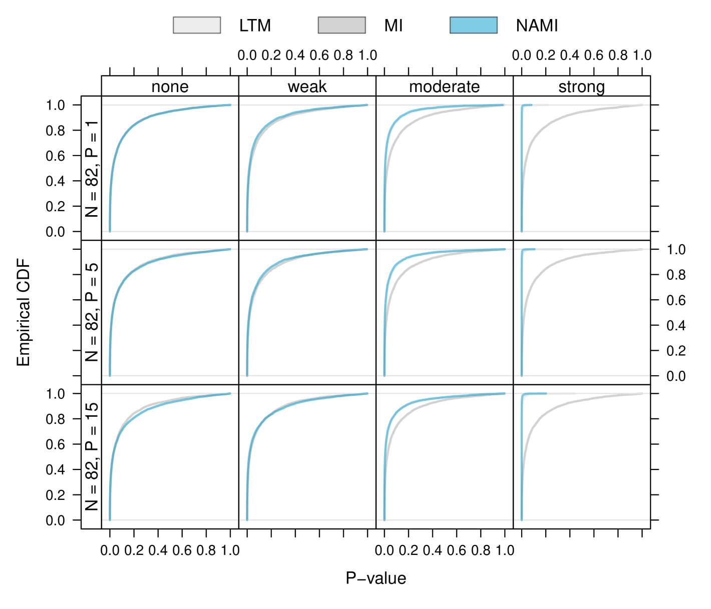
Figure S. 3: Empirical experiments for normally distributed outcome under $\tau=0.5$: P-value distribution for test against null hypothesis $H_{0}:\tau=\tau_{\text{\boldmath$x$}}=0$ obtained from unadjusted marginal inference (MI), nonparanormal adjusted marginal inference (NAMI), or from linear transformation models (LTM) under varying prognostic strengths of covariate $X_{1}$ (in columns) and increasing number of noise covariates ($P$, in rows).

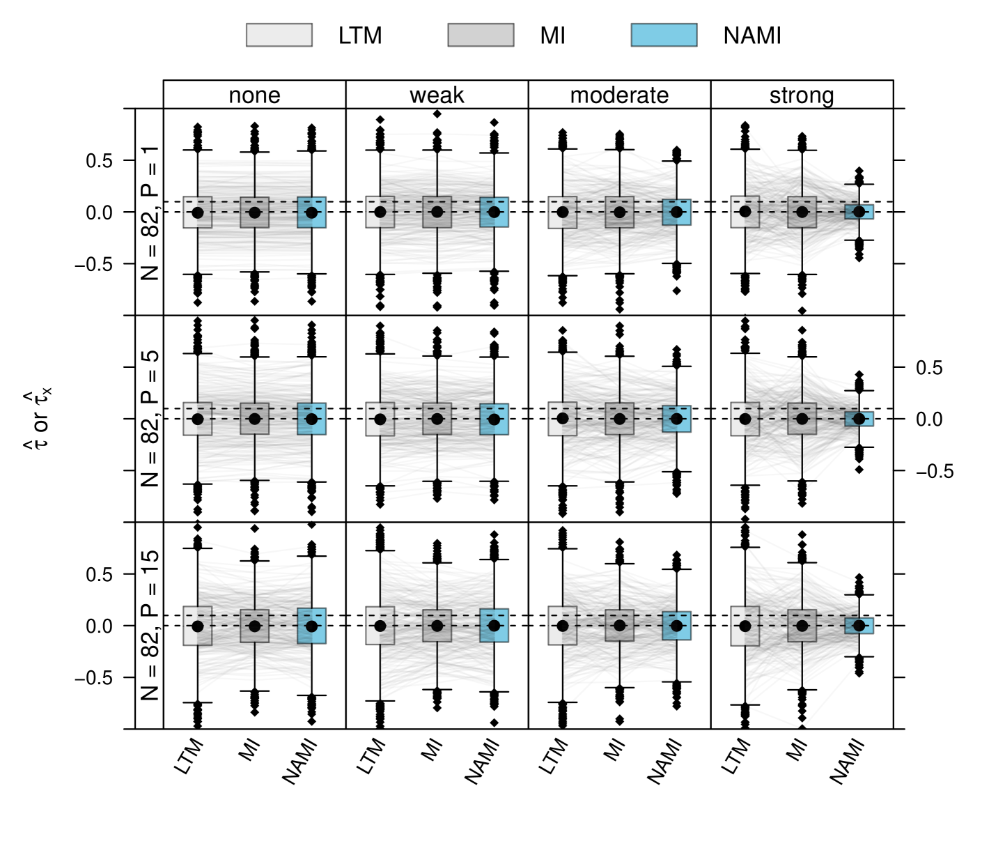
Figure S. 4: Empirical experiments for normally distributed outcome under $\tau=0$ (dashed lines): Distribution of treatment effect estimates $\hat{\tau}$ of Cohen’s $d$ obtained from unadjusted marginal inference (MI) and nonparanormal adjusted marginal inference (NAMI), and effect estimates of $\hat{\tau}_{\text{\boldmath$x$}}$ by linear transformation models (LTM) under varying prognostic strengths of covariate $X_{1}$ (in columns) and increasing number of noise covariates ($P$, in rows).

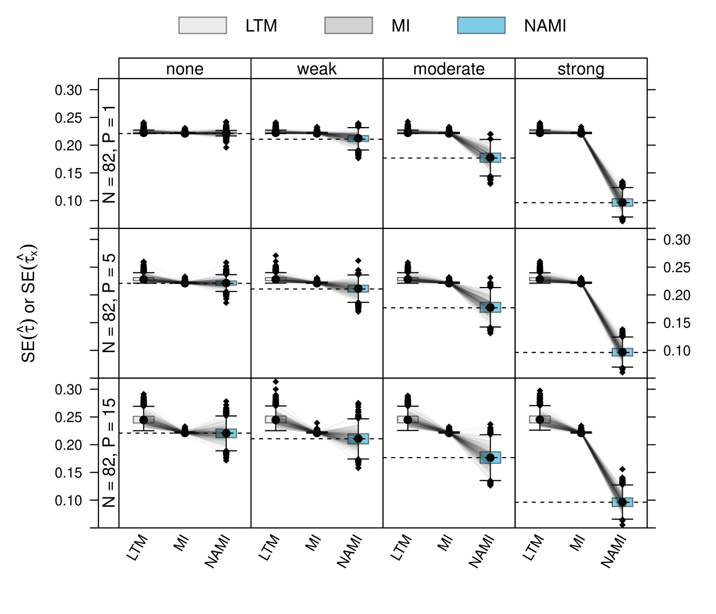
Figure S. 5: Empirical experiments for normally distributed outcome under $\tau=0$: Distribution of standard errors of treatment effect estimates $\hat{\tau}$ of Cohen’s $d$ obtained from unadjusted marginal inference (MI) and nonparanormal adjusted marginal inference (NAMI), and effect estimates of $\hat{\tau}_{\text{\boldmath$x$}}$ by linear transformation models (LTM) under varying prognostic strengths of covariate $X_{1}$ (in columns) and increasing number of noise covariates ($P$, in rows). Standard errors were computed by inverting the numerically determined negative Hessian. The dashed lines correspond to the theoretical standard errors $\text{SE}(\tau,\lambda)$ given true $\tau=0$ and differing true $\lambda$ (Lemma 2).

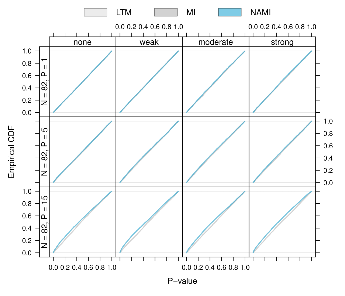
Figure S. 6: Empirical experiments for normally distributed outcome under $\tau=0$: P-value distribution for test against null hypothesis $H_{0}:\tau=\tau_{\text{\boldmath$x$}}=0$ obtained from unadjusted marginal inference (MI), nonparanormal adjusted marginal inference (NAMI), or from linear transformation models (LTM) under varying prognostic strengths of covariate $X_{1}$ (in columns) and increasing number of noise covariates ($P$, in rows).

Table S. 1: Empirical experiments: Empirical size for different outcome types obtained from linear transformation models (LTM), unadjusted marginal inference (MI), and nonparanormal adjusted marginal inference (NAMI) under varying prognostic strength of covariate $X_{1}$ (in columns) and varying number of (noise) covariates ($P$, in rows). For binary and survival outcomes, analysis was also performed for the standardisation approaches of Zhang et al. (2008) and Lu and Tsiatis (2008) (YSTD), and Ye et al. (2024) (LRCL). For survival outcomes, results are only shown for heavy censoring.

			Size
DGP	Algorithm	P	none	weak	moderate	strong
normal	LTM	P = 1	0.051	0.051	0.054	0.056
		P = 5	0.066	0.060	0.062	0.057
		P = 15	0.081	0.091	0.076	0.084
	MI	P = 1	0.050	0.052	0.059	0.052
		P = 5	0.056	0.053	0.054	0.057
		P = 15	0.055	0.059	0.053	0.054
	NAMI	P = 1	0.052	0.052	0.058	0.060
		P = 5	0.067	0.061	0.066	0.062
		P = 15	0.083	0.097	0.080	0.090
binary	LTM	P = 1	0.050	0.056	0.050	0.049
		P = 5	0.054	0.053	0.052	0.056
		P = 15	0.054	0.051	0.058	0.054
	MI	P = 1	0.050	0.062	0.050	0.048
		P = 5	0.054	0.048	0.053	0.048
		P = 15	0.053	0.047	0.061	0.042
	NAMI	P = 1	0.050	0.058	0.051	0.052
		P = 5	0.055	0.051	0.053	0.059
		P = 15	0.055	0.053	0.062	0.059
	YSTD	P = 1	0.050	0.057	0.051	0.050
		P = 5	0.055	0.052	0.054	0.060
		P = 15	0.054	0.052	0.061	0.064
survival	LTM	P = 1	0.051	0.053	0.061	0.095
		P = 5	0.054	0.054	0.068	0.099
		P = 15	0.066	0.063	0.079	0.119
	MI	P = 1	0.048	0.053	0.049	0.053
		P = 5	0.052	0.045	0.051	0.051
		P = 15	0.051	0.046	0.057	0.050
	NAMI	P = 1	0.049	0.052	0.050	0.053
		P = 5	0.052	0.048	0.054	0.057
		P = 15	0.065	0.057	0.066	0.080
	LRCL	P = 1	0.046	0.050	0.048	0.051
		P = 5	0.056	0.048	0.054	0.057
		P = 15	0.069	0.064	0.068	0.065
	YSTD	P = 1	0.051	0.055	0.045	0.049
		P = 5	0.062	0.055	0.058	0.059
		P = 15	0.092	0.081	0.084	0.072

Table S. 2: Empirical experiments under $\tau=0$ and $\tau=0.5$: Frequency of prognostic covariate $X_{1}$ being identified as the most prognostic one over 5000 replications obtained from nonparanormal adjusted marginal inference (NAMI) under varying prognostic strengths of covariate $X_{1}$ (in columns) and increasing number of noise covariates ($P$, in rows).

				Ranking
DGP	Algorithm	P	$\tau$	weak	moderate	strong
normal	NAMI	P = 5	0	0.774	0.999	1.000
			0.5	0.766	0.999	1.000
		P = 15	0	0.278	0.864	1.000
			0.5	0.290	0.859	1.000
binary	NAMI	P = 5	0	0.978	1.000	1.000
			0.5	0.975	1.000	1.000
		P = 15	0	0.792	1.000	1.000
			0.5	0.782	1.000	1.000
survival	NAMI	P = 5	0	0.948	1.000	1.000
			0.5	0.934	1.000	1.000
		P = 15	0	0.665	0.998	1.000
			0.5	0.654	0.997	1.000

C.3 Binary outcome

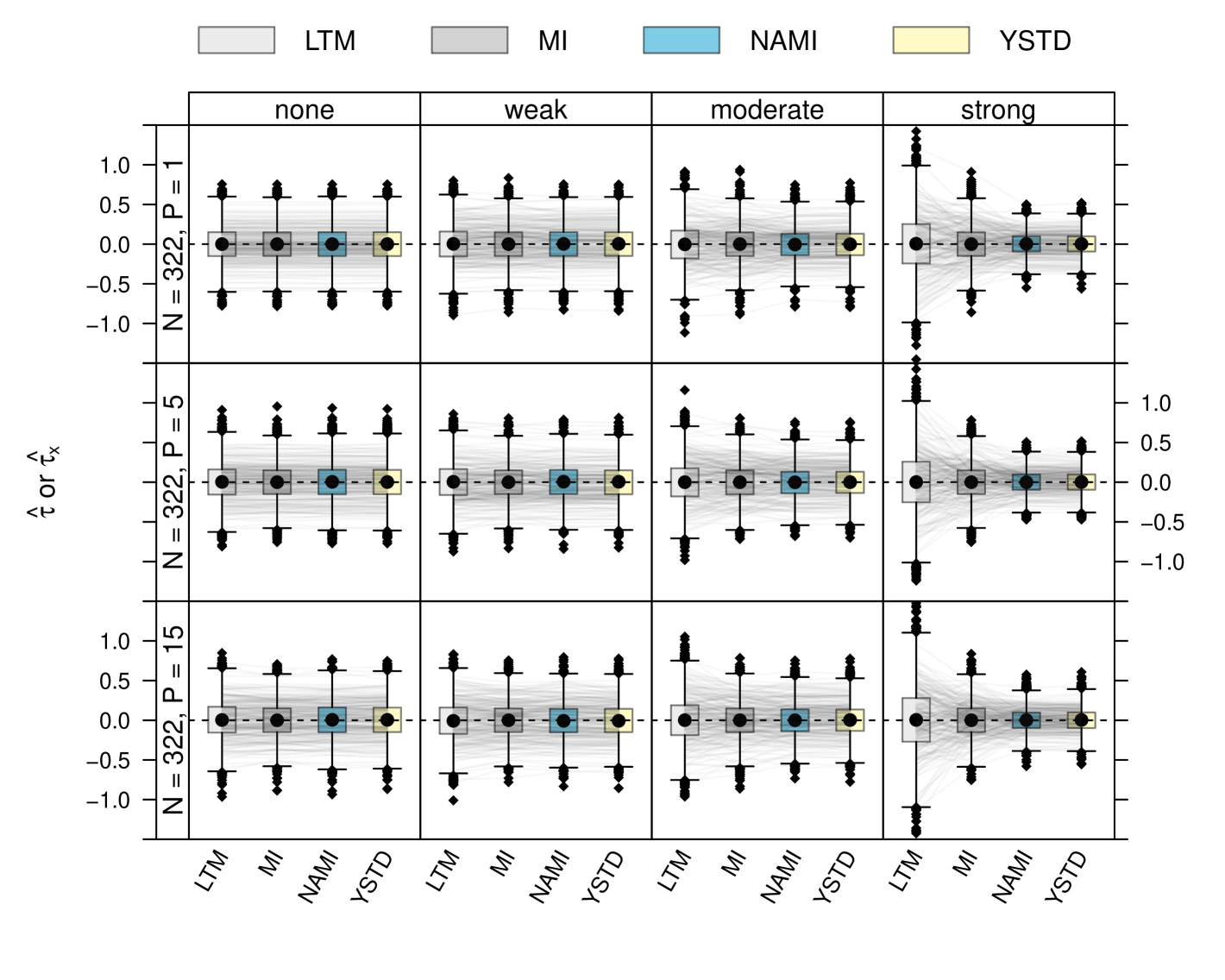
Figure S. 7: Empirical experiments for binary outcome and $\tau=0$ (dashed lines): Distribution of log-odds ratio treatment effect estimates $\tau$ obtained from unadjusted marginal inference (MI), nonparanormal adjusted marginal inference (NAMI), or the standardisation approach of Zhang et al. (2008) (YSTD), and effect estimates of $\hat{\tau}_{\text{\boldmath$x$}}$ by linear transformation models (LTM) under varying prognostic strengths of covariate $X_{1}$ (in columns) and increasing number of (noise) covariates ($P$, in rows).

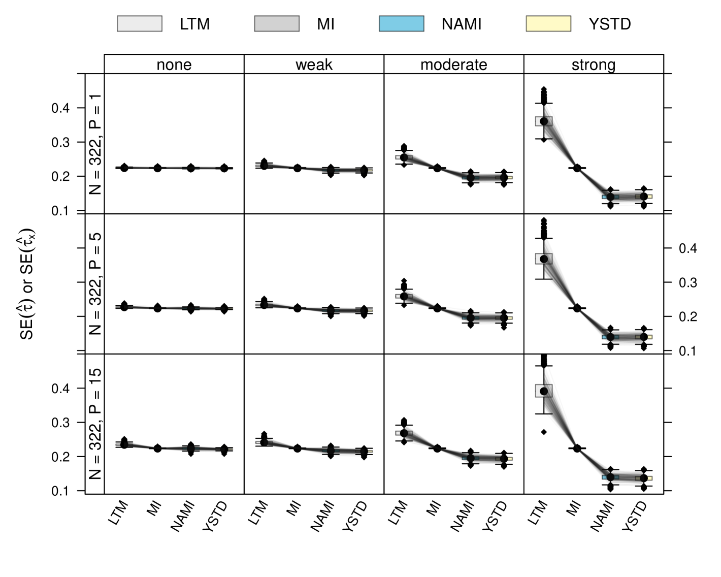
Figure S. 8: Empirical experiments for binary outcome and $\tau=0$: Distribution of standard errors of log-odds ratio treatment effect estimates $\hat{\tau}$ obtained from unadjusted marginal inference (MI), nonparanormal adjusted marginal inference (NAMI), or the standardisation approach of Zhang et al. (2008) (YSTD), and effect estimates of $\hat{\tau}_{\text{\boldmath$x$}}$ by linear transformation models (LTM) under varying prognostic strengths of covariate $X_{1}$ (in columns) and increasing number of (noise) covariates ($P$, in rows). Standard errors were computed by inverting the numerically determined negative Hessian.

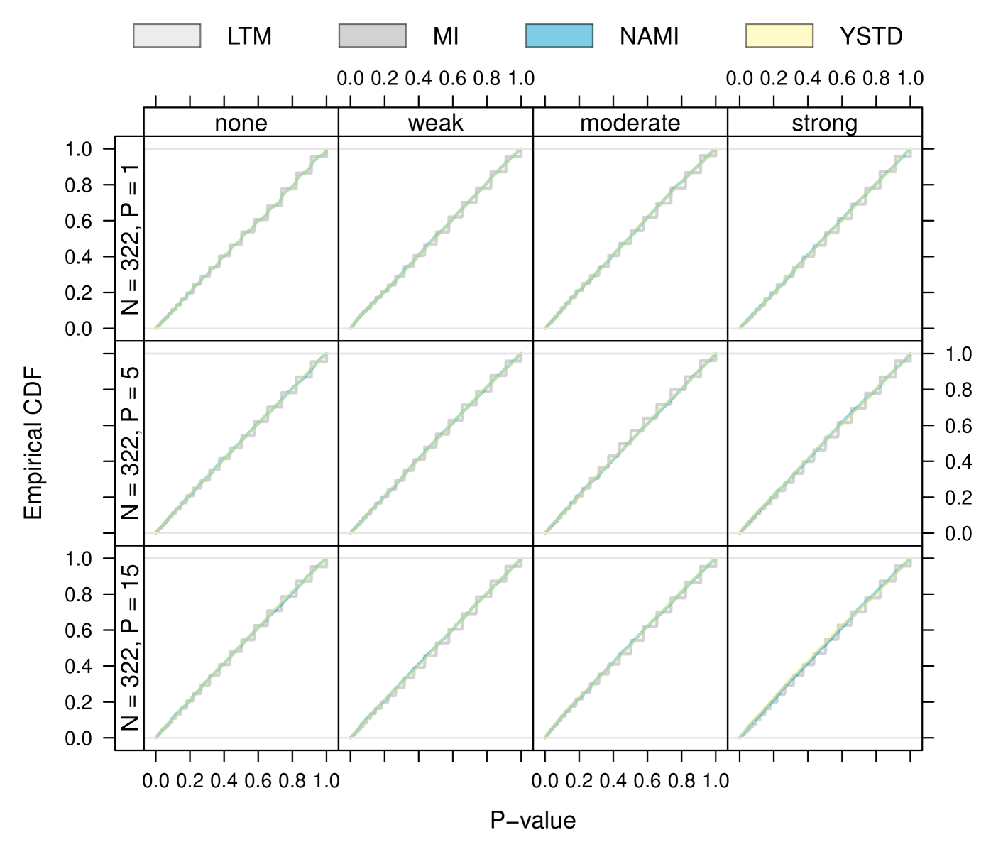
Figure S. 9: Empirical experiments for binary outcome and $\tau=0$: P-value distribution for test of null hypothesis $H_{0}:\tau=\tau_{\text{\boldmath$x$}}=0$ obtained from unadjusted marginal inference (MI), nonparanormal adjusted marginal inference (NAMI), the standardisation approach of Zhang et al. (2008) (YSTD), or from linear transformation models (LTM) under varying prognostic strengths of covariate $X_{1}$ (in columns) and increasing number of noise covariates ($P$, in rows).

Figure S. 10: Empirical experiments for binary outcome and $\tau=0.5$ (dashed lines): Distribution of log-odds ratio treatment effect estimates $\tau$ obtained from unadjusted marginal inference (MI), nonparanormal adjusted marginal inference (NAMI), or the standardisation approach of Zhang et al. (2008) (YSTD), and effect estimates of $\hat{\tau}_{\text{\boldmath$x$}}$ by linear transformation models (LTM) under varying prognostic strengths of covariate $X_{1}$ (in columns) and increasing number of (noise) covariates ($P$, in rows).

Figure S. 11: Empirical experiments for binary outcome and $\tau=0.5$: Distribution of standard errors of log-odds ratio treatment effect estimates $\hat{\tau}$ obtained from unadjusted marginal inference (MI), nonparanormal adjusted marginal inference (NAMI), or the standardisation approach of Zhang et al. (2008) (YSTD), and effect estimates of $\hat{\tau}_{\text{\boldmath$x$}}$ by linear transformation models (LTM) under varying prognostic strengths of covariate $X_{1}$ (in columns) and increasing number of (noise) covariates ($P$, in rows). Standard errors were computed by inverting the numerically determined negative Hessian.

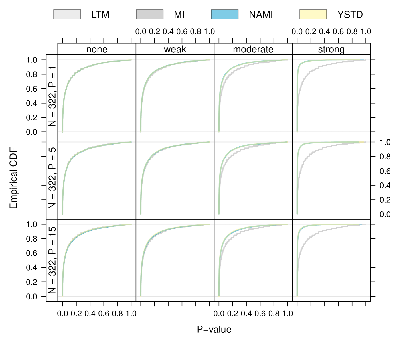
Figure S. 12: Empirical experiments for binary outcome and $\tau=0.5$: P-value distribution for test of null hypothesis $H_{0}:\tau=\tau_{\text{\boldmath$x$}}=0$ obtained from unadjusted marginal inference (MI), nonparanormal adjusted marginal inference (NAMI), the standardisation approach of Zhang et al. (2008) (YSTD), or from linear transformation models (LTM) under varying prognostic strengths of covariate $X_{1}$ (in columns) and increasing number of noise covariates ($P$, in rows).

C.4 Survival outcome

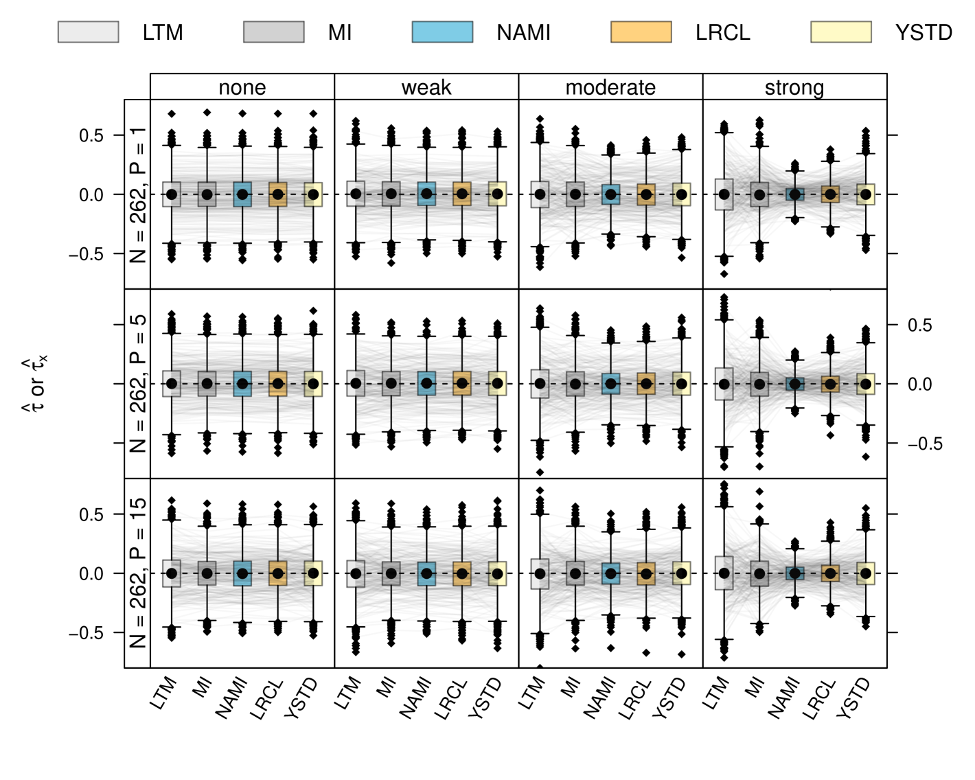
Figure S. 13: Empirical experiments for survival outcome under low censoring for $\tau=0$ (dashed lines): Distribution of log-hazard ratio treatment effect estimates $\hat{\tau}$ obtained from unadjusted marginal inference (MI), nonparanormal adjusted marginal inference (NAMI), or the standardisation approaches of Ye et al. (2024) (LRCL) and Lu and Tsiatis (2008) (YSTD), and effect estimates of $\hat{\tau}_{\text{\boldmath$x$}}$ by linear transformation models (LTM) under varying prognostic strengths of covariate $X_{1}$ (in columns) and increasing number of noise covariates ($P$, in rows). Standard errors were computed by inverting the numerically determined negative Hessian.

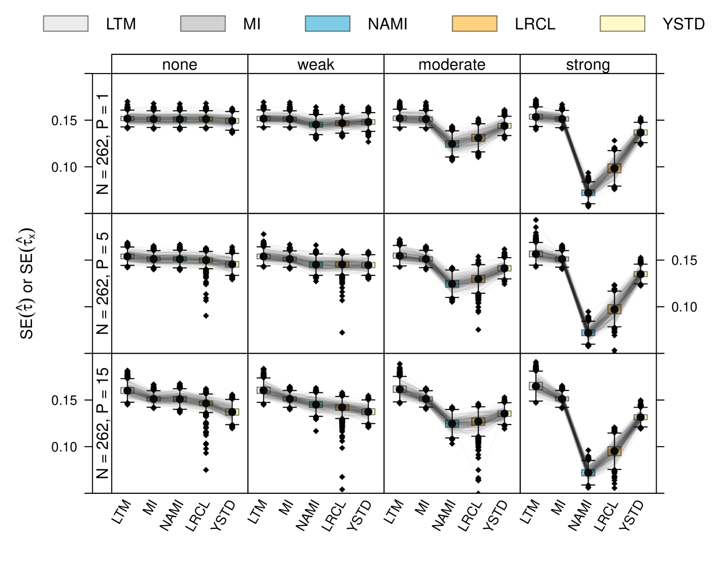
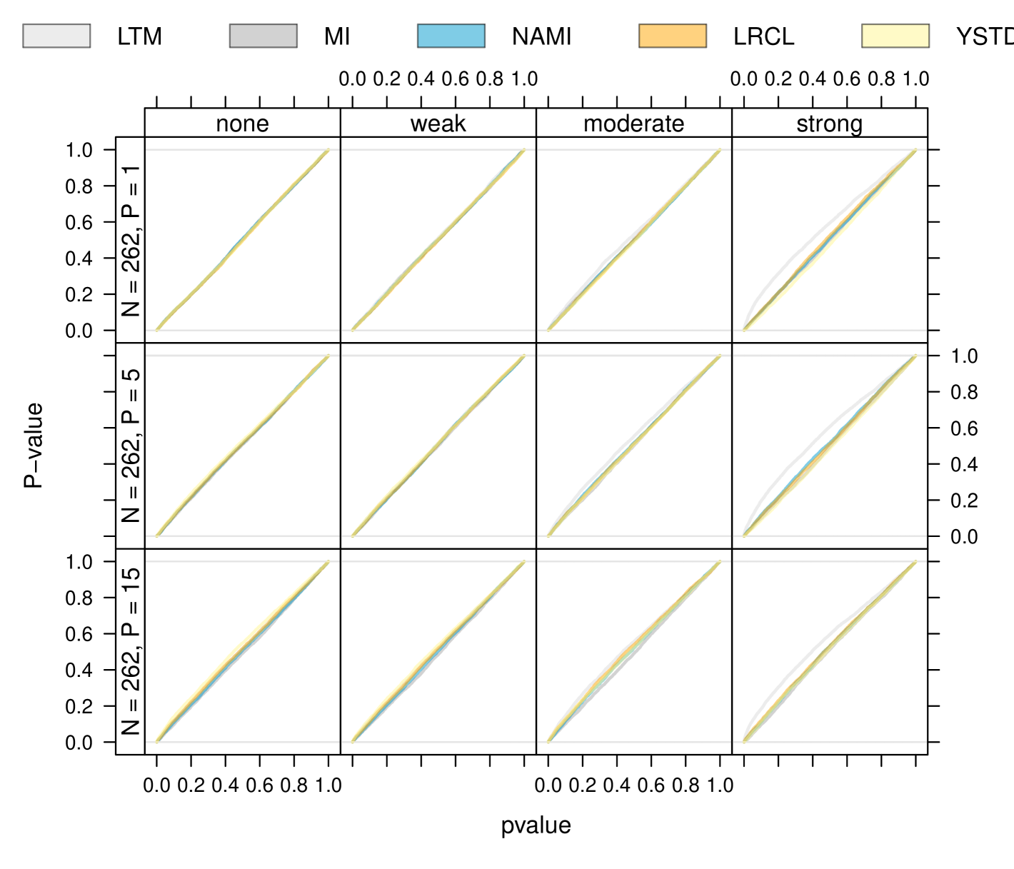
Figure S. 14: Empirical experiments for survival outcome under low censoring and $\tau=0$: Distribution of standard errors of log-hazard ratio treatment effect estimates $\hat{\tau}$ obtained from unadjusted marginal inference (MI), nonparanormal adjusted marginal inference (NAMI), or the standardisation approaches of Ye et al. (2024) (LRCL) and Lu and Tsiatis (2008) (YSTD), and effect estimates of $\hat{\tau}_{\text{\boldmath$x$}}$ by linear transformation models (LTM) under varying prognostic strengths of covariate $X_{1}$ (in columns) and increasing number of noise covariates ($P$, in rows). Standard errors were computed by inverting the numerically determined negative Hessian.

Figure S. 15: Empirical experiments for survival outcome under low censoring and $\tau=0$: P-value distribution for test against null hypothesis $H_{0}:\tau=\tau_{\text{\boldmath$x$}}=0$ obtained from unadjusted marginal inference (MI), nonparanormal adjusted marginal inference (NAMI), or the standardisation approaches of Ye et al. (2024) (LRCL) and Lu and Tsiatis (2008) (YSTD), and effect estimates of $\hat{\tau}_{\text{\boldmath$x$}}$ by linear transformation models (LTM) under varying prognostic strengths of covariate $X_{1}$ (in columns) and increasing number of noise covariates ($P$, in rows).

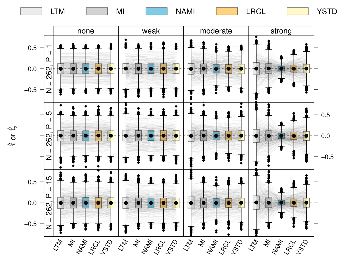
Figure S. 16: Empirical experiments for survival outcome under mild censoring for $\tau=0$ (dashed lines): Distribution of standard errors of log-hazard ratio treatment effect estimates $\hat{\tau}$ obtained from unadjusted marginal inference (MI), nonparanormal adjusted marginal inference (NAMI), or the standardisation approaches of Ye et al. (2024) (LRCL) and Lu and Tsiatis (2008) (YSTD), and effect estimates of $\hat{\tau}_{\text{\boldmath$x$}}$ by linear transformation models (LTM) under varying prognostic strengths of covariate $X_{1}$ (in columns) and increasing number of noise covariates ($P$, in rows). Standard errors were computed by inverting the numerically determined negative Hessian.

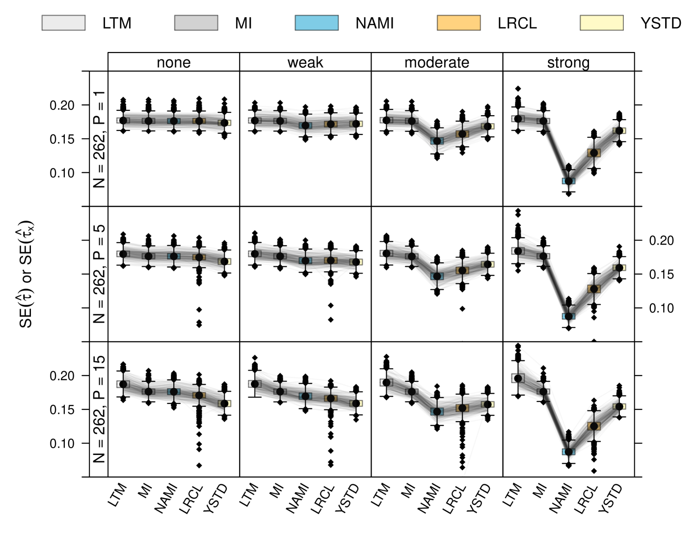
Figure S. 17: Empirical experiments for survival outcome under mild censoring and $\tau=0$: Distribution of standard errors of log-hazard ratio treatment effect estimates $\hat{\tau}$ obtained from unadjusted marginal inference (MI), nonparanormal adjusted marginal inference (NAMI), or the standardisation approaches of Ye et al. (2024) (LRCL) and Lu and Tsiatis (2008) (YSTD), and effect estimates of $\hat{\tau}_{\text{\boldmath$x$}}$ by linear transformation models (LTM) under varying prognostic strengths of covariate $X_{1}$ (in columns) and increasing number of noise covariates ($P$, in rows). Standard errors were computed by inverting the numerically determined negative Hessian.

Figure S. 18: Empirical experiments for survival outcome under mild censoring and $\tau=0$: P-value distribution for test against null hypothesis $H_{0}:\tau=\tau_{\text{\boldmath$x$}}=0$ obtained from unadjusted marginal inference (MI), nonparanormal adjusted marginal inference (NAMI), or the standardisation approaches of Ye et al. (2024) (LRCL) and Lu and Tsiatis (2008) (YSTD), and effect estimates of $\hat{\tau}_{\text{\boldmath$x$}}$ by linear transformation models (LTM) under varying prognostic strengths of covariate $X_{1}$ (in columns) and increasing number of noise covariates ($P$, in rows).

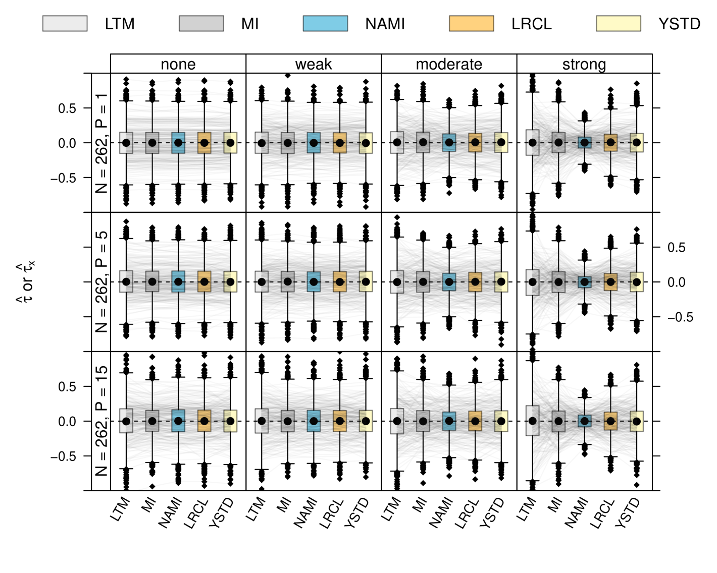
Figure S. 19: Empirical experiments for survival outcome under heavy censoring for $\tau=0$ (dashed lines): Distribution of standard errors of log-hazard ratio treatment effect estimates $\hat{\tau}$ obtained from unadjusted marginal inference (MI), nonparanormal adjusted marginal inference (NAMI), or the standardisation approaches of Ye et al. (2024) (LRCL) and Lu and Tsiatis (2008) (YSTD), and effect estimates of $\hat{\tau}_{\text{\boldmath$x$}}$ by linear transformation models (LTM) under varying prognostic strengths of covariate $X_{1}$ (in columns) and increasing number of noise covariates ($P$, in rows). Standard errors were computed by inverting the numerically determined negative Hessian.

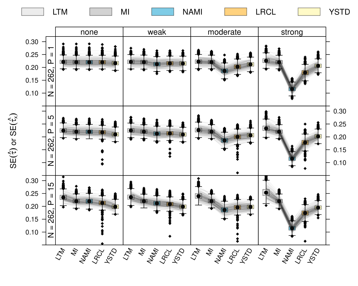
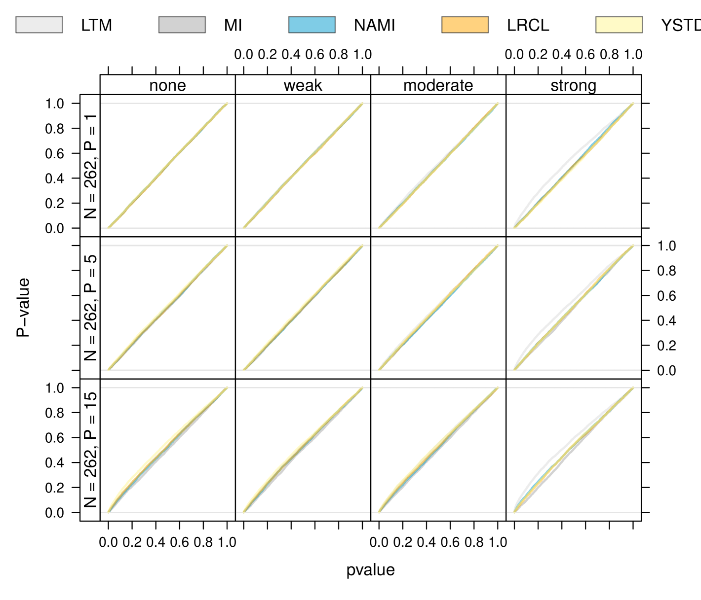
Figure S. 20: Empirical experiments for survival outcome under heavy censoring and $\tau=0$: Distribution of standard errors of log-hazard ratio treatment effect estimates $\hat{\tau}$ obtained from unadjusted marginal inference (MI), nonparanormal adjusted marginal inference (NAMI), or the standardisation approaches of Ye et al. (2024) (LRCL) and Lu and Tsiatis (2008) (YSTD), and effect estimates of $\hat{\tau}_{\text{\boldmath$x$}}$ by linear transformation models (LTM) under varying prognostic strengths of covariate $X_{1}$ (in columns) and increasing number of noise covariates ($P$, in rows). Standard errors were computed by inverting the numerically determined negative Hessian.

Figure S. 21: Empirical experiments for survival outcome under heavy censoring and $\tau=0$: P-value distribution for test against null hypothesis $H_{0}:\tau=\tau_{\text{\boldmath$x$}}=0$ obtained from unadjusted marginal inference (MI), nonparanormal adjusted marginal inference (NAMI), or the standardisation approaches of Ye et al. (2024) (LRCL) and Lu and Tsiatis (2008) (YSTD), and effect estimates of $\hat{\tau}_{\text{\boldmath$x$}}$ by linear transformation models (LTM) under varying prognostic strengths of covariate $X_{1}$ (in columns) and increasing number of noise covariates ($P$, in rows).

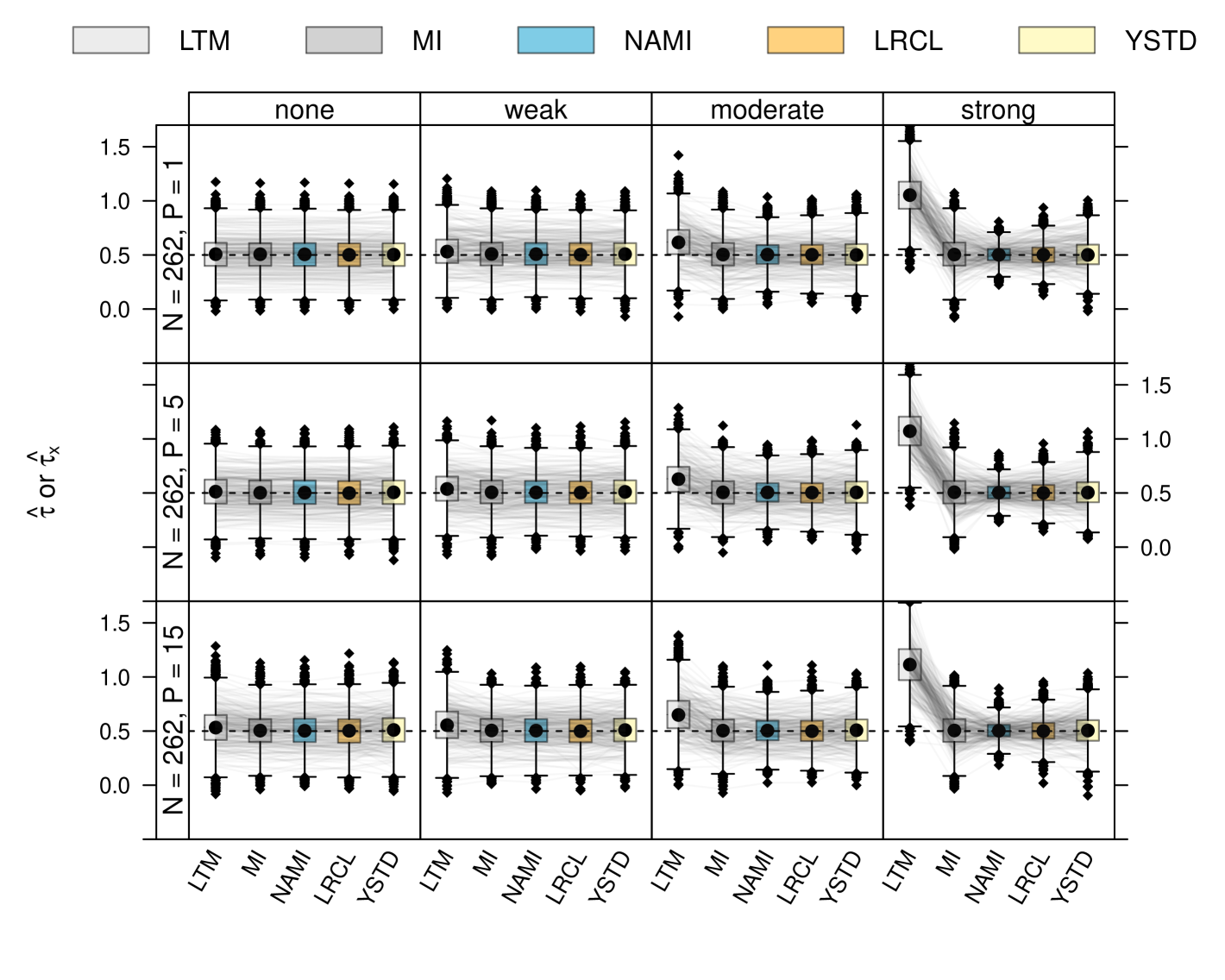
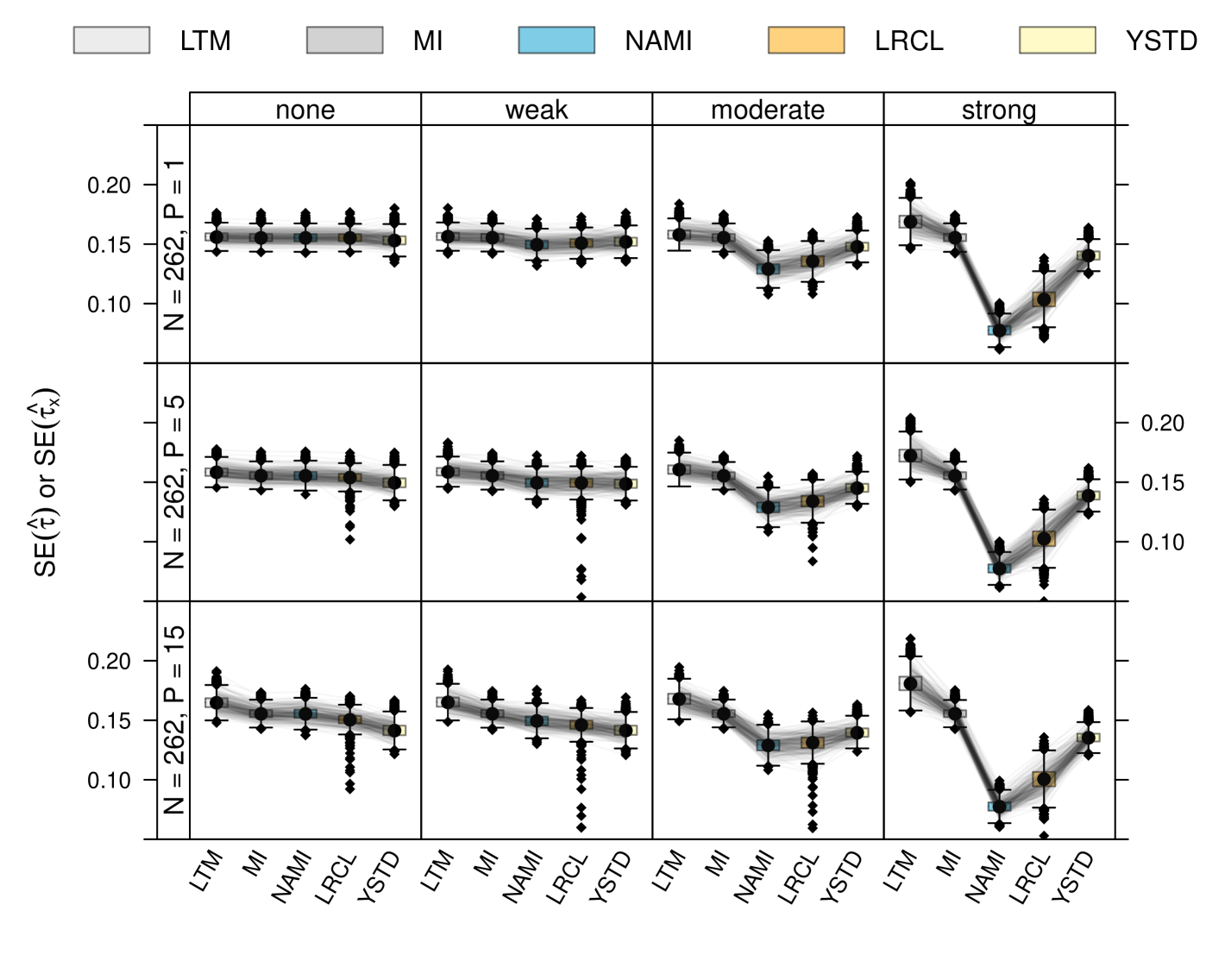
Figure S. 22: Empirical experiments for survival outcome under low censoring and $\tau=0.5$ (dashed lines): Distribution of log-hazard ratio treatment effect estimates $\tau$ obtained from unadjusted marginal inference (MI), nonparanormal adjusted marginal inference (NAMI), or the standardisation approaches of Ye et al. (2024) (LRCL) and Lu and Tsiatis (2008) (YSTD), and effect estimates of $\hat{\tau}_{\text{\boldmath$x$}}$ by linear transformation models (LTM) under varying prognostic strengths of covariate $X_{1}$ (in columns) and increasing number of noise covariates ($P$, in rows).

Figure S. 23: Empirical experiments for survival outcome under low censoring and $\tau=0.5$: Distribution of standard errors of log-hazard ratio treatment effect estimates $\hat{\tau}$ obtained from unadjusted marginal inference (MI), nonparanormal adjusted marginal inference (NAMI), or the standardisation approaches of Ye et al. (2024) (LRCL) and Lu and Tsiatis (2008) (YSTD), and effect estimates of $\hat{\tau}_{\text{\boldmath$x$}}$ by linear transformation models (LTM) under varying prognostic strengths of covariate $X_{1}$ (in columns) and increasing number of noise covariates ($P$, in rows). Standard errors were computed by inverting the numerically determined negative Hessian.

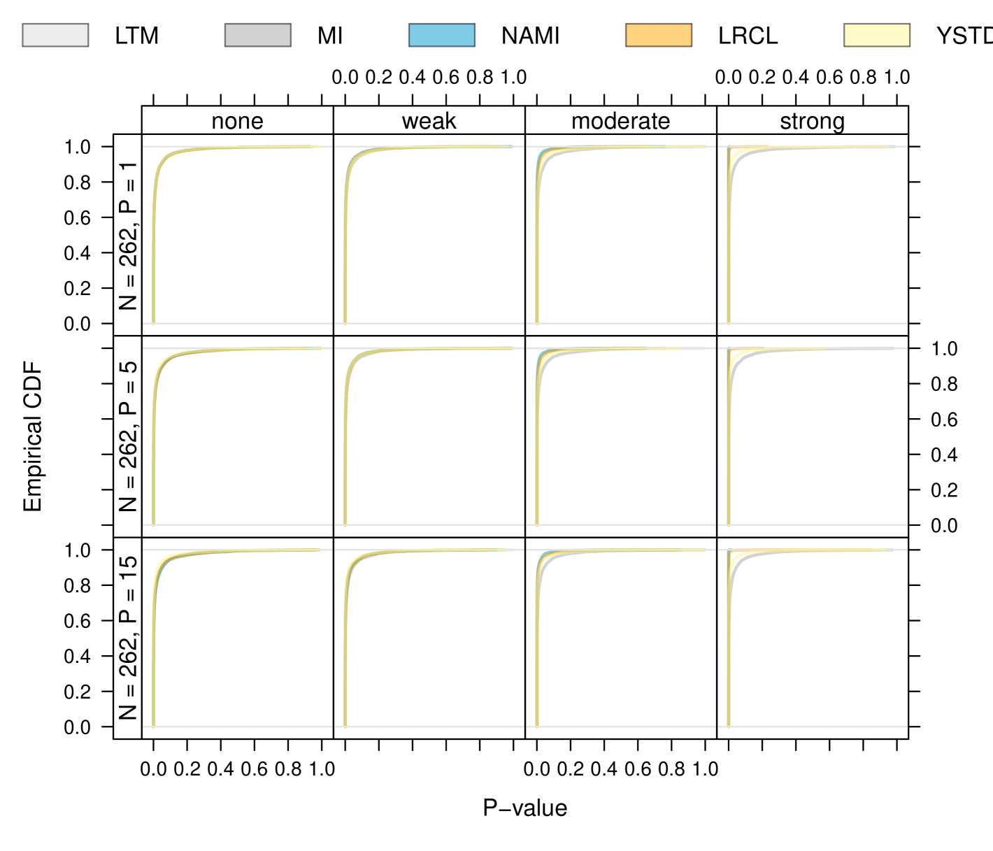
Figure S. 24: Empirical experiments for survival outcome under low censoring and $\tau=0.5$: P-value distribution for test against null hypothesis $H_{0}:\tau=\tau_{\text{\boldmath$x$}}=0.5$ obtained from unadjusted marginal inference (MI), nonparanormal adjusted marginal inference (NAMI), or the standardisation approaches of Ye et al. (2024) (LRCL) and Lu and Tsiatis (2008) (YSTD), and effect estimates of $\hat{\tau}_{\text{\boldmath$x$}}$ by linear transformation models (LTM) under varying prognostic strengths of covariate $X_{1}$ (in columns) and increasing number of noise covariates ($P$, in rows).

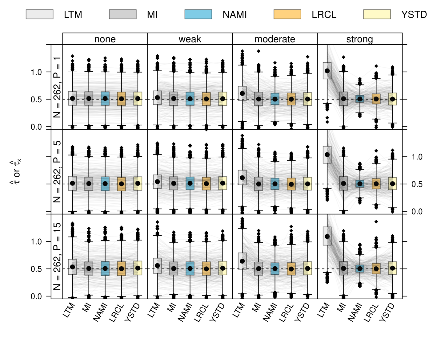
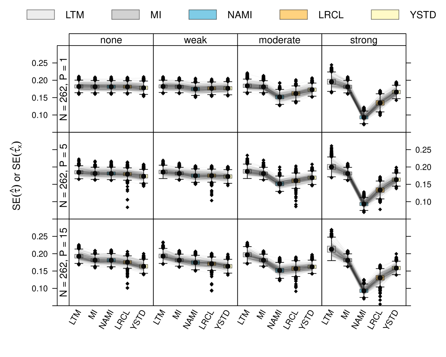
Figure S. 25: Empirical experiments for survival outcome under mild censoring and $\tau=0.5$ (dashed lines): Distribution of log-hazard ratio treatment effect estimates $\tau$ obtained from unadjusted marginal inference (MI), nonparanormal adjusted marginal inference (NAMI), or the standardisation approaches of Ye et al. (2024) (LRCL) and Lu and Tsiatis (2008) (YSTD), and effect estimates of $\hat{\tau}_{\text{\boldmath$x$}}$ by linear transformation models (LTM) under varying prognostic strengths of covariate $X_{1}$ (in columns) and increasing number of noise covariates ($P$, in rows).

Figure S. 26: Empirical experiments for survival outcome under mild censoring and $\tau=0.5$: Distribution of standard errors of log-hazard ratio treatment effect estimates $\hat{\tau}$ obtained from unadjusted marginal inference (MI), nonparanormal adjusted marginal inference (NAMI), or the standardisation approaches of Ye et al. (2024) (LRCL) and Lu and Tsiatis (2008) (YSTD), and effect estimates of $\hat{\tau}_{\text{\boldmath$x$}}$ by linear transformation models (LTM) under varying prognostic strengths of covariate $X_{1}$ (in columns) and increasing number of noise covariates ($P$, in rows). Standard errors were computed by inverting the numerically determined negative Hessian.

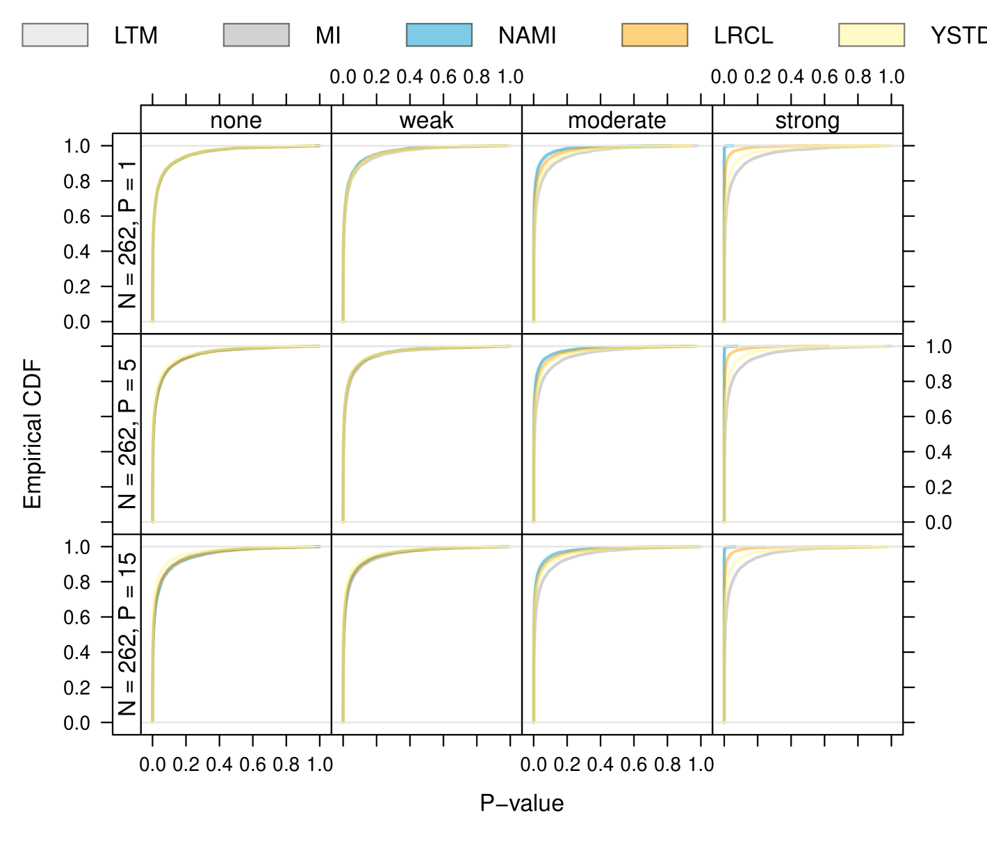
Figure S. 27: Empirical experiments for survival outcome under mild censoring and $\tau=0.5$: P-value distribution for test against null hypothesis $H_{0}:\tau=\tau_{\text{\boldmath$x$}}=0.5$ obtained from unadjusted marginal inference (MI), nonparanormal adjusted marginal inference (NAMI), or the standardisation approaches of Ye et al. (2024) (LRCL) and Lu and Tsiatis (2008) (YSTD), and effect estimates of $\hat{\tau}_{\text{\boldmath$x$}}$ by linear transformation models (LTM) under varying prognostic strengths of covariate $X_{1}$ (in columns) and increasing number of noise covariates ($P$, in rows).

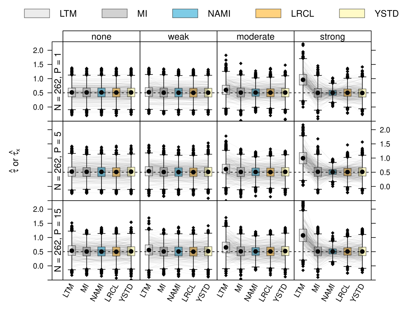
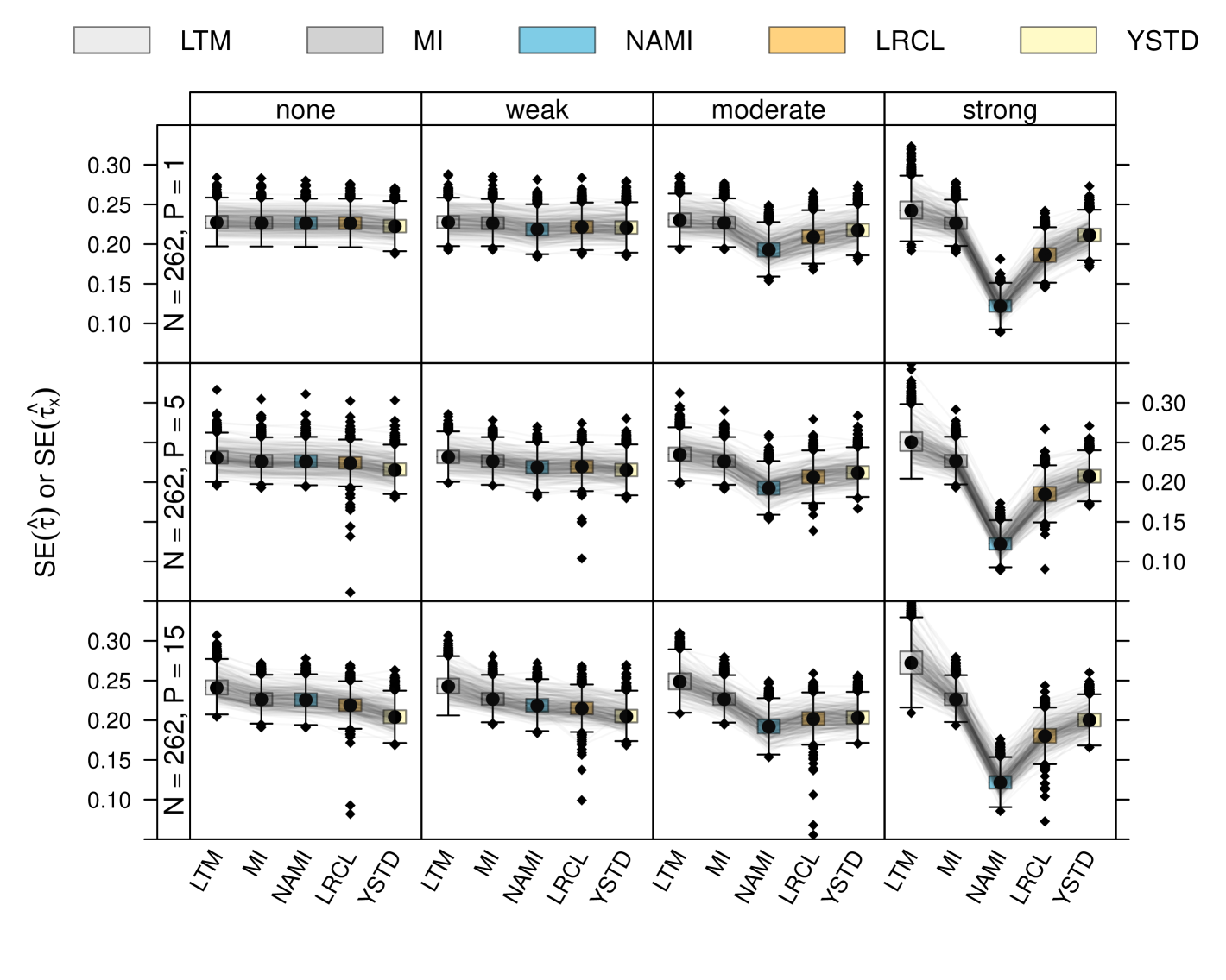
Figure S. 28: Empirical experiments for survival outcome under heavy censoring and $\tau=0.5$ (dashed lines): Distribution of log-hazard ratio treatment effect estimates $\tau$ obtained from unadjusted marginal inference (MI), nonparanormal adjusted marginal inference (NAMI), or the standardisation approaches of Ye et al. (2024) (LRCL) and Lu and Tsiatis (2008) (YSTD), and effect estimates of $\hat{\tau}_{\text{\boldmath$x$}}$ by linear transformation models (LTM) under varying prognostic strengths of covariate $X_{1}$ (in columns) and increasing number of noise covariates ($P$, in rows).

Figure S. 29: Empirical experiments for survival outcome under heavy censoring and $\tau=0.5$: Distribution of standard errors of log-hazard ratio treatment effect estimates $\hat{\tau}$ obtained from unadjusted marginal inference (MI), nonparanormal adjusted marginal inference (NAMI), or the standardisation approaches of Ye et al. (2024) (LRCL) and Lu and Tsiatis (2008) (YSTD), and effect estimates of $\hat{\tau}_{\text{\boldmath$x$}}$ by linear transformation models (LTM) under varying prognostic strengths of covariate $X_{1}$ (in columns) and increasing number of noise covariates ($P$, in rows). Standard errors were computed by inverting the numerically determined negative Hessian.

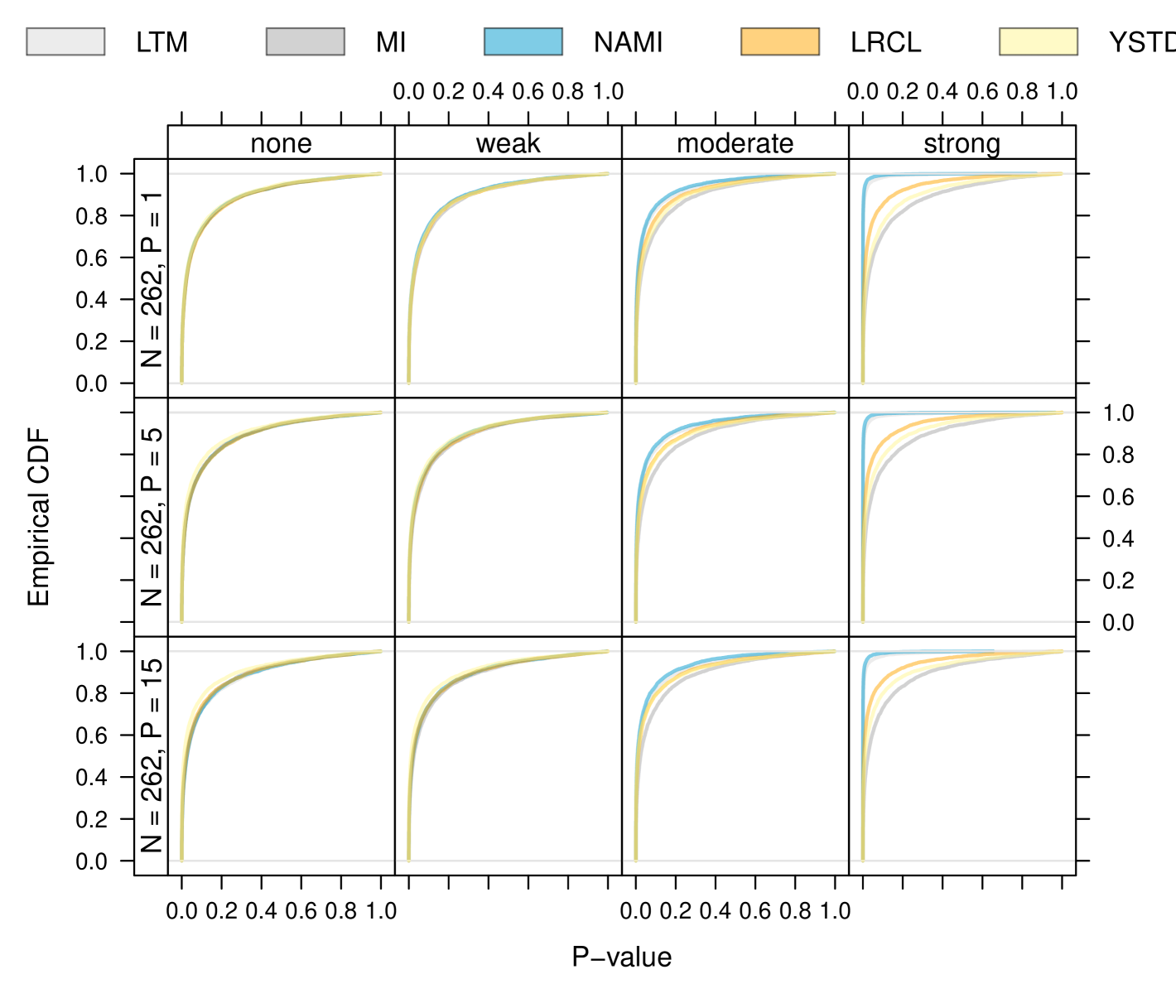
Figure S. 30: Empirical experiments for survival outcome under heavy censoring and $\tau=0.5$: P-value distribution for test against null hypothesis $H_{0}:\tau=\tau_{\text{\boldmath$x$}}=0.5$ obtained from unadjusted marginal inference (MI), nonparanormal adjusted marginal inference (NAMI), or the standardisation approaches of Ye et al. (2024) (LRCL) and Lu and Tsiatis (2008) (YSTD), and effect estimates of $\hat{\tau}_{\text{\boldmath$x$}}$ by linear transformation models (LTM) under varying prognostic strengths of covariate $X_{1}$ (in columns) and increasing number of noise covariates ($P$, in rows).

Appendix D Model misspecification

We illustrate the effect of model misspecification using the $\Gamma$-frailty model by Aalen et al. (2015). For one $\Gamma$-distributed covariate $X_{1}$, the survival time $Y$ is given by a frailty model being identical to a conditional Weibull model:

$$X_{1} \sim \Gamma(\eta,\eta),\quad\mathbb{E}(X_{1})=1,\mathbb{V}(X_{1})=\eta^{-1}$$

$$\mathbb{P}(Y\leq y\mid W=w,X_{1}=x_{1}) = 1-\exp(-x_{1}\exp(\vartheta_{1}+\vartheta_{2}\log(y)+\tau_{\text{\boldmath$x$}}w))$$

$$= \text{cloglog}^{-1}(\vartheta_{1}+\vartheta_{2}\log(y)+\tau_{\text{\boldmath$x$}}w+\log(x_{1})).$$

For conditional log-hazard ratios $\tau_{\text{\boldmath$x$}}\neq 0$, the marginal distribution $Y\mid W=w$ features a time-dependent hazard ratio function which, as a function of the variance $\mathbb{V}(X_{1})=\eta^{-1}\rightarrow\infty$ tends to one (Aalen et al., 2015). Thus, a marginal Cox proportional hazards model $\text{cloglog}^{-1}(h(y)+\tau w)$ is misspecified.

For $\tau_{\text{\boldmath$x$}}=0$, the marginal Cox model $\text{cloglog}^{-1}(h(y)+\tau w)$ is overparameterised, as $\tau=0$. The joint distribution of $h_{1}(X_{1})$ and $h(Y)$ can, however, not be expressed by a Gaussian copula. Therefore, nonparanormal adjusted marginal inference is misspecified under both situations.

We compare the correctly specified conditional Weibull model (LTM), marginal inference (MI, a marginal Cox model comparing the two groups), nonparanormal adjusted marginal inference (NAMI, based on the same Cox model) and the standardization approach of Ye et al. (2024) (LRCL) for $N_{1}=N_{0}=131$, $\tau_{\text{\boldmath$x$}}=0,0.5$ (as in the simulation study in Section 3), and $\vartheta_{1}=1,\vartheta_{2}=4$. For $5000$ simulation runs, we estimate the corresponding treatment effect parameters and also perform a Wald test against the null hypothesis $H_{0}:\tau=\tau_{\text{\boldmath$x$}}=0$.

The distribution of the parameter estimates is given in Figure S. 31. For $\tau_{\text{\boldmath$x$}}=0$, all three procedures are nearly unbiased, and the parameter variances of NAMI and LRCL are reduced. For $\tau_{\text{\boldmath$x$}}=0.5$, MI, NAMI and LRCL are biased towards zero, whereas the conditional estimate by the Weibull model is right on target.

We were in addition interested in the Wald tests’ $p$-value distributions (Figure S. 32). Under the null hypothesis (left panel), the two correctly specified models (MI and LTM) correspond to nearly perfectly uniform $p$-value distributions. The same could be observed for LRCL reflecting that the method does not rely on any distributional assumptions and is therefore less prone to model misspecifications (Ye et al., 2024). The distribution of the misspecified NAMI is stochastically too large, leading to a conservative test. Under the alternative (right panel), the correctly specified Weibull model is most powerful. MI leads to much fewer rejections at all levels. Covariate adjustment in misspecified NAMI, however, is more powerful than the analysis by MI and LRCL, but less powerful than the conditional test.

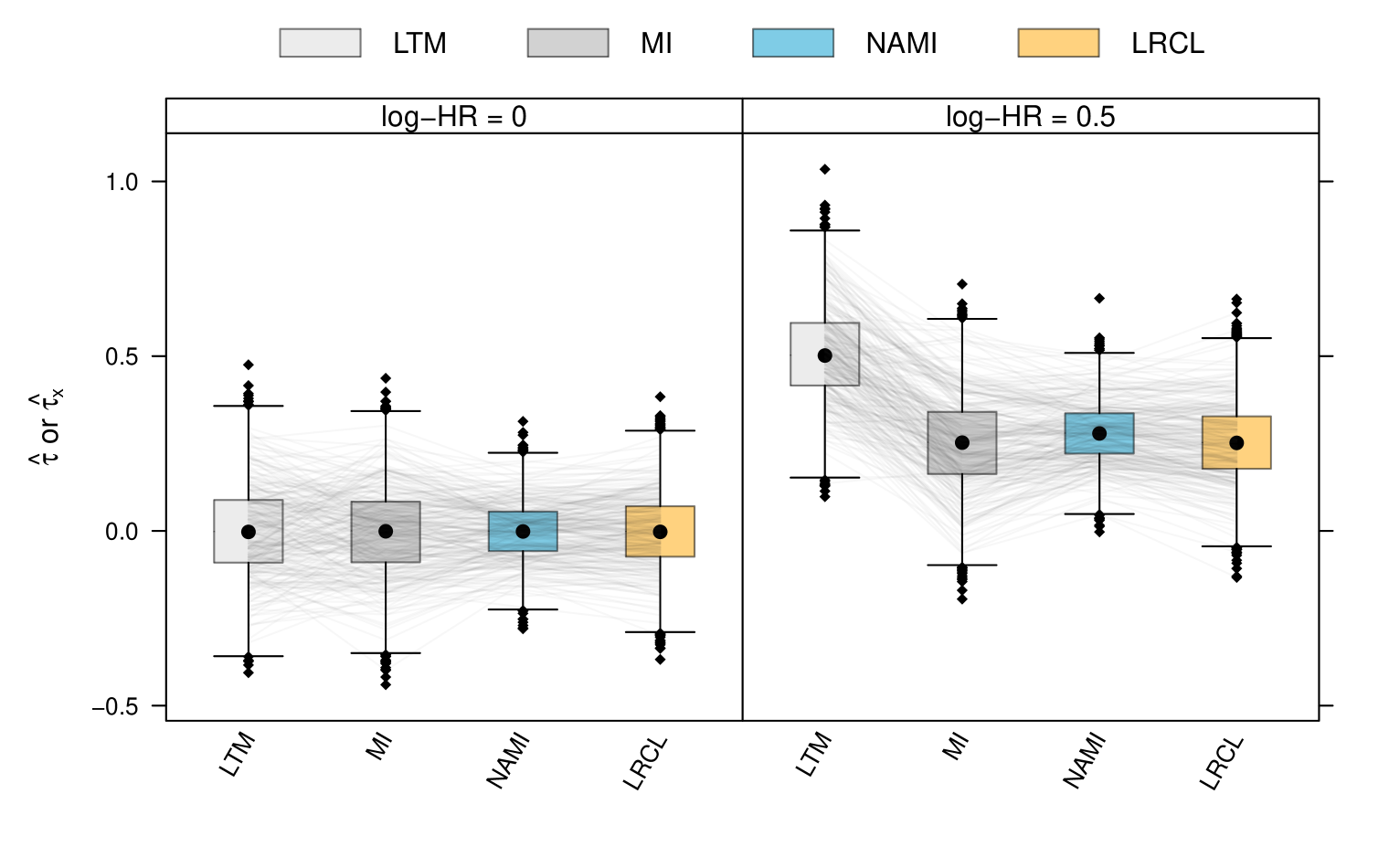
Figure S. 31: Empirical experiments for misspecified models: Distribution of log-hazard ratio treatment effect estimates $\tau$ obtained from unadjusted marginal inference (MI), nonparanormal adjusted marginal inference (NAMI), the standardization approach of Ye et al. (2024) and the correctly linear transformation models (LTM, Weibull model).

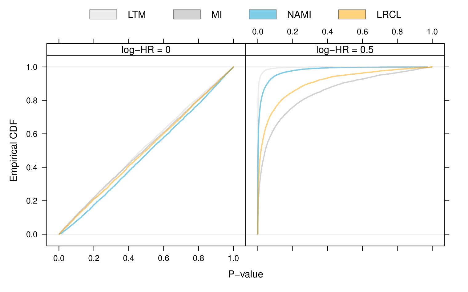
Figure S. 32: Empirical experiments for misspecified models: P-value distribution for test against null hypothesis $H_{0}:\tau=\tau_{\text{\boldmath$x$}}=0$ obtained from unadjusted marginal inference (MI), nonparanormal adjusted marginal inference (NAMI), the standardization approach of Ye et al. (2024) and the correctly linear transformation models (LTM, Weibull model).

References

- Aalen et al. (2015) Aalen OO, Cook RJ, Røysland K (2015). “Does Cox Analysis of a Randomized Survival Study Yield a Causal Treatment Effect?” Lifetime Data Analysis, 21(4), 579–593. 10.1007/s10985-015-9335-y.
- Bannick et al. (2024) Bannick M, Ye T, Yi Y, Bian F (2024). RobinCar: Robust Inference for Covariate Adjustment in Randomized Clinical Trials. 10.32614/CRAN.package.RobinCar. \proglangR package version 0.3.2.
- Box and Cox (1964) Box GEP, Cox DR (1964). “An Analysis of Transformations.” Journal of the Royal Statistical Society: Series B (Statistical Methodology), 26(2), 211–252. 10.1111/j.2517-6161.1964.tb00553.x.
- Daniel et al. (2021) Daniel R, Zhang J, Farewell D (2021). “Making Apples From Oranges: Comparing Noncollapsible Effect Estimators and Their Standard Errors After Adjustment for Different Covariate Sets.” Biometrical Journal, 63(3), 528–557. 10.1002/bimj.201900297.
- Dette et al. (2014) Dette H, Van Hecke R, Volgushev S (2014). “Some Comments on Copula-Based Regression.” Journal of the American Statistical Association, 109(507), 1319–1324. 10.1080/01621459.2014.916577.
- Doi et al. (2022) Doi SA, Abdulmajeed J, Xu C (2022). “Redefining Effect Modification.” Journal of Evidence-Based Medicine, 15(3), 192–197. 10.1111/jebm.12495.
- Farouki (2012) Farouki RT (2012). “The Bernstein Polynomial Basis: A Centennial Retrospective.” Computer Aided Geometric Design, 29(6), 379–419. 10.1016/j.cagd.2012.03.001.
- Fleiss et al. (2003) Fleiss JL, Levin B, Paik MC (2003). Statistical Methods for Rates and Proportions. John Wiley & Sons Inc., Hoboken, New Jersey, U.S.A. 10.1002/0471445428.
- Hothorn (2024) Hothorn T (2024). “On Nonparanormal Likelihoods.” Technical report, arXiv 2408.17346. 10.48550/arXiv.2408.17346.
- Hothorn et al. (2025) Hothorn T, Barbanti L, Siegfried S, Kook L (2025). tram: Transformation Models. 10.32614/CRAN.package.tram. \proglangR package version 1.2-1.
- Hothorn et al. (2018) Hothorn T, Möst L, Bühlmann P (2018). “Most Likely Transformations.” Scandinavian Journal of Statistics, 45(1), 110–134. 10.1111/sjos.12291.
- Juraska et al. (2022) Juraska M, Gilbert PB, Lu X, Zhang M, Davidian M, Tsiatis AA (2022). speff2trial: Semiparametric Efficient Estimation for a Two-Sample Treatment Effect. 10.32614/CRAN.package.speff2trial. \proglangR package version 1.0.5.
- Kennedy et al. (2023) Kennedy EH, Balakrishnan S, Wasserman LA (2023). “Semiparametric Counterfactual Density Estimation.” Biometrika, 110(4), 875–896. 10.1093/biomet/asad017.
- Klein et al. (2022) Klein N, Hothorn T, Barbanti L, Kneib T (2022). “Multivariate Conditional Transformation Models.” Scandinavian Journal of Statistics, 49, 116–142. 10.1111/sjos.12501.
- Lang and Bischl (2023) Lang M, Bischl B (2023). batchtools: Tools for Computation on Batch Systems. 10.32614/CRAN.package.batchtools. \proglangR package version 0.9.17.
- Liu et al. (2009) Liu H, Lafferty J, Wasserman L (2009). “The Nonparanormal: Semiparametric Estimation of High Dimensional Undirected Graphs.” Journal of Machine Learning Research, 10(80), 2295–2328. URL http://jmlr.org/papers/v10/liu09a.html.
- Lu and Tsiatis (2008) Lu X, Tsiatis AA (2008). “Improving the Efficiency of the Log-Rank Test Using Auxiliary Covariates.” Biometrika, 95(3), 679–694. 10.1093/biomet/asn003.
- Martinussen and Vansteelandt (2013) Martinussen T, Vansteelandt S (2013). “On Collapsibility and Confounding Bias in Cox and Aalen Regression Models.” Lifetime Data Analysis, 19(3), 279–296. 10.1007/s10985-013-9242-z.
- McKelvey and Zavoina (1975) McKelvey RD, Zavoina W (1975). “A Statistical Model for the Analysis of Ordinal Level Dependent Variables.” The Journal of Mathematical Sociology, 4(1), 103–120. 10.1080/0022250X.1975.9989847.