Heterogeneity Matters even More in Distributed Learning: Study from Generalization Perspective

Abstract

In this paper, we investigate the effect of data heterogeneity across clients on the performance of distributed learning systems, i.e., one-round Federated Learning, as measured by the associated generalization error. Specifically, $K$ clients have each $n$ training samples generated independently according to a possibly different data distribution and their individually chosen models are aggregated by a central server. We study the effect of the discrepancy between the clients’ data distributions on the generalization error of the aggregated model. First, we establish in-expectation and tail upper bounds on the generalization error in terms of the distributions. In part, the bounds extend the popular Conditional Mutual Information (CMI) bound which was developed for the centralized learning setting, i.e., $K=1$, to the distributed learning setting with arbitrary number of clients $K\geq 1$. Then, we use a connection with information theoretic rate-distortion theory to derive possibly tighter lossy versions of these bounds. Next, we apply our lossy bounds to study the effect of data heterogeneity across clients on the generalization error for distributed classification problem in which each client uses Support Vector Machines (D-SVM). In this case, we establish explicit generalization error bounds which depend explicitly on the data heterogeneity degree. It is shown that the bound gets smaller as the degree of data heterogeneity across clients gets higher, thereby suggesting that D-SVM generalizes better when the dissimilarity between the clients’ training samples is bigger. This finding, which goes beyond D-SVM, is validated experimentally through a number of experiments.

I Introduction

Amajor focus of machine learning research over recent years has been the study of statistical learning algorithms when applied in distributed (network or graph) settings. In part, this is due to the emergence of new applications in which resources are constrained, data is distributed, or the need to preserve privacy. Examples of such algorithms include the now popular Federated Learning [1], the Split Learning of [2] or the so-called in-network learning of [3, 4]. Despite its importance, however, little is known about the generalization guarantees of distributed statistical learning algorithms, including lack of proper definitions [5, 6]. Notable exceptions include the related works [7, 8, 9, 10, 11] and [12].

The lack of understanding of what really controls generalization in distributed learning settings is even more pronounced when the (training) data exhibits some degree of heterogeneity across participating clients or devices. That is, when the underlying probability distributions (if there exist such distributions!) vary across those clients. In fact, the question of the effect of data heterogeneity on the performance of statistical learning algorithms is not yet fully understood even from a convergence rate perspective, a line of work which is more studied comparatively. For example, while it has been reported that non-independently and/or non-identically distributed (non-IID) data slow down convergence in FL-type algorithms [13, 14, 15] optimal rates are still unknown in general; and, how that slowness relates to the behavior of the generalization error is yet un-explored.

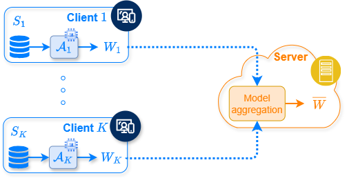
Figure 1: Studied distributed learning problem

In this paper, we study the distributed learning system shown in Figure 1. Here, there are $K$ clients; each having access to a training dataset $S_{k}=\{Z_{k,1},\dots,Z_{k,n}\}\in\mathcal{Z}^{n}$ of size $n$, where the data samples $\{Z_{k,1},\dots,Z_{k,n}\}$ are generated independently from each other and from other clients’ training samples according to a probability distribution $\mu_{k}$. The probability distributions $\{\mu_{k}\}_{k=1}^{K}$ are possibly distinct, i.e., heterogeneous across clients. In the special case in which $\mu_{k}=\mu$ for all $k=1,\ldots,K$, we will refer to the setting as being homogeneous. Client $k$ applies a possibly stochastic learning algorithm $A_{k}:\mathcal{Z}^{n}_{k}\rightarrow\mathcal{W}_{k}$. This induces a conditional distribution $P_{W_{k}|S_{k}}$, which together with $\mu_{k}$ induce the joint dataset-hypothesis distribution $P_{W_{k},S_{k}}=\mu_{k}^{\otimes n}P_{W_{k}|S_{k}}$. The server receives $(W_{1},\ldots,W_{K})$ and picks the hypothesis $\overline{W}$ as the arithmetic average

$$\overline{W}=\frac{1}{K}\sum\limits_{k=1}^{K}W_{k}.$$ (1)

We investigate the effect of the discrepancy between the clients’ data distributions on the generalization performance of the aggregated model $\overline{W}$. In particular, for given loss function $\ell:\mathcal{Z}\times\mathcal{W}\to[0,1]$ used to evaluate the quality of the prediction and a proper definition of the generalization error (see formal definitions in Section II), we ask the following question:

How does the generalization error of the aggregated model $\overline{W}$ evolve as function of a measure of discrepancy between the data distributions $\mu_{1},\ldots,\mu_{K}$ ?

I-A Main contributions

The main contributions of this paper are as follows:

• We establish (general) in-expectation and tail upper bounds on the generalization error in terms of the distributions $(\mu_{1},\ldots,\mu_{K})$. In part, the bounds extend the Conditional Mutual Information (CMI) bound, which was developed for the centralized learning, i.e., $K=1$ in [16], to the distributed learning setting of Figure 1.

• We use a connection between the theory of generalization of statistical learning algorithms and information theoretic rate-distortion theory that was introduced in [9] and subsequently used and elaborated on in [17, 18, 19], to obtain possibly tighter lossy versions of these bounds. Furthermore, we also provide improved bounds that are based on Jensen-Shannon divergence.

• We apply our established lossy bounds to study the effect of data heterogeneity across clients on the generalization error for a distributed classification problem in which each client uses Support Vector Machines (SVM). In this case, we establish in-expectation generalization bounds that depend explicitly on the degree of data heterogeneity across clients; and, by comparing them, we show that the bounds get better (i.e., smaller) as the degree of data heterogeneity across clients increases. Also, the bounds increase as the total variation between the distributions becomes smaller.

• We provide experiments on various datasets that validate the results of this paper for both feature- and label heterogeneity, for D-SVM and beyond. This includes synthetic data with feature heterogeneity across clients, noisy MNIST with feature heterogeneity across clients and MNIST with label heterogeneity across clients.

I-B Relation to prior art

On the line of work investigating the effect of heterogeneity on the performance of distributed and FL-type learning systems, most related to our work here is [20] and, to a lesser extent, [21]. In [20], the authors analyze the generalization error of FL by means of algorithmic stability. Also, they report experimental results for a 10-class MNIST type classification problem, which show that, when trained with FedAvg, SCAFFOLD, and FedProx, label heterogeneity across clients increases the generalization error. Comparatively, we are mostly concerned with feature heterogeneity across clients (except in Experiment 2 in Section VIII-B). Also, our approach to studying the generalization error and the resulting bounds, which apply to a one-round scenario, are different in nature, being rate-distortion theoretic. The interested reader may also refer to, e.g.,  [22, 22, 23, 24], which study the different, but somewhat related, question of the effect of data heterogeneity on the convergence rates of algorithms such as LocalSGD and SCAFFOLD.

I-C Notation

Upper case letters denote random variables, e.g., $X$; lower case letters denote realizations of random variables, e.g., $x$; and calligraphic letters denote sets, e.g., $\mathcal{X}$. The probability distribution of a random variable $X$ is denoted as $P_{X}$ and its support set as $\operatorname{supp}(P_{X})$. For probability distributions $P$ and $Q$ defined over a common measurable space $\mathcal{X}$ such that $Q$ is absolutely continuous with respect to $P$ (i.e., $Q\ll P$), the relative entropy between $Q$ and $P$, also called the Kullback-Leibler (KL) divergence, is given by $D_{KL}(Q\|P)\coloneqq\mathbb{E}_{Q}\Big{[}\log\Big{(}\frac{dQ}{dP}\Big{)}\Big{]}$. If $Q$ is not absolutely continuous with respect to $P$, the Radon-Nikodym derivative $\frac{dQ}{dP}$ is undefined and we set $D_{KL}(Q\|P)=\infty$. The Shannon mutual information (MI) between two random variables $X$ and $Y$ with joint distribution $P_{X,Y}$ and marginals $P_{X}$ and $P_{Y}$ is given by

$$I(X;Y)=D_{KL}(P_{X,Y}\parallel P_{X}P_{Y}).$$

Conditional mutual information, given a possibly correlated variable $Z$, is denoted as $I(X;Y|Z)$ and given by

$$I(X;Y|Z)=\mathbb{E}_{P_{Z}}\left[D_{KL}\left(P_{X,Y|Z}\parallel P_{X|Z}P_{Y|Z}\right)\right].$$ (2)

For $n\in\mathbb{N}$, the notation $[n]$ denotes the set $\{1,\dots,n\}$. Also, $\mathbbm{1}_{\{\cdot\}}$ designates the indicator function. Finally, a set of random variables $\{X_{1},\dots,X_{n}\}$ is sometimes abbreviated as $X_{[n]}$. Finally, for $(a,b)\in\mathbb{R}^{2}$, $[a,b]^{+}=\text{max}(a,b)$.

II System model and preliminaries

Consider the distributed learning system shown in Figure 1. As mentioned, there are $K$ clients; each with a training dataset $S_{k}=\{Z_{k,1},\dots,Z_{k,n}\}\in\mathcal{Z}^{n}$ of size $n$, whose samples $\{Z_{k,1},\dots,Z_{k,n}\}$ are generated independently from each other and from other clients’ training samples according to some probability distribution $\mu_{k}$. The probability distributions $\{\mu_{k}\}_{k=1}^{K}$ are allowed to vary across clients; and we refer to such setting as being heterogeneous. This is opposed to homogeneous data setting (across clients) in which $\mu_{k}=\mu$ for all $k=1,\ldots,K$. For example, for classification tasks we set $Z_{k,i}=(X_{k,i},Y_{k,i})$, where $X_{k,i}$ denotes the feature sample and $Y_{k,i}$ is the associated label. Client $k$ applies a possibly stochastic learning algorithm $A_{k}:\mathcal{Z}^{n}_{k}\rightarrow\mathcal{W}_{k}$. This induces a conditional distribution $P_{W_{k}|S_{k}}$, which together with $\mu_{k}$ induce the joint dataset-hypothesis distribution $P_{W_{k},S_{k}}=\mu_{k}^{\otimes n}P_{W_{k}|S_{k}}$. The server receives the hypotheses $(W_{1},\ldots,W_{K})$ and picks the hypothesis $\overline{W}$ as the arithmetic average given by (1). We use a loss function $\ell:\mathcal{Z}\times\mathcal{W}\to[0,1]$ to evaluate the quality of the prediction. For a given value $\overline{w}$ of aggregated model, how well it performs on the training dataset of Client $k$ is evaluated using the empirical risk

$$\hat{\mathcal{L}}_{k}(S_{k},\overline{w})=\frac{1}{n}\sum\nolimits_{i=1}^{n}\ell(Z_{k,i},\overline{w});$$ (3)

and how well it does on test data distributed according to $\mu_{k}$ is evaluated as

$$\mathcal{L}_{k}(\overline{w})=\mathbb{E}_{Z\sim\mu_{k}}[\ell(Z_{k},\overline{w})].$$ (4)

Setting

$${\operatorname{gen}}_{k}(\overline{w})=\mathcal{L}_{k}(\overline{w})-\hat{\mathcal{L}}_{k}(S_{k},\overline{w}),$$ (5)

in this paper, for the dataset $S_{[K]}=(S_{1},\ldots,S_{K})$ we measure the generalization error of aggregated hypothesis $\overline{W}$ as the average (over clients)

$$\operatorname{gen}(S_{[K]},\overline{W})=\frac{1}{K}\sum\nolimits_{k=1}^{K}\operatorname{gen}_{k}(\overline{W}).$$ (6)

As we already mentioned in the Introduction section, we study the effect of the discrepancy between the data distributions on the generalization error (6) of the aggregated model (1). Then, we apply the found results, to an example D-SVM, to gain insights onto which of two training procedures (among heterogeneous data across clients or homogeneous data across clients) yields an aggregated model $\overline{W}=(W_{1}+\ldots+W_{K})/K$ that generalizes better to unseen data during test time – for fair comparison, the test samples are generated from the same distribution for both settings.

For convenience, we define the following symmetry property which will be instrumental throughout.

Definition 1 (Symmetric Priors).

Let $\sigma:[2n]\to[2n]$ be an arbitrary permutation of the set $\{1,\ldots,2n\}$. For a generic vector $U^{2n}=(U_{1},U_{2},\ldots,U_{2n})$, we set $\sigma(U^{2n})\coloneqq\left(U_{\sigma(1)},\cdots,U_{\sigma(2n)}\right)$.

• Type-I symmetry: Define Type-I permutations as the set of permutations $\sigma:[2n]\to[2n]$ with the property that $\{\sigma(i),\sigma(i+n)\}=\{i,i+n\}$ for all $i=1,\ldots,n$. A conditional distribution (prior) $Q(W\lvert V^{2n})$ is said to possess type-I symmetry if $Q(W|\sigma(V^{2n})$ is invariant under any type-I permutation $\sigma:[2n]\to[2n]$.

• Type-II symmetry: The conditional prior $\mathbf{Q}(W|V^{2n})$ is said to satisfy Type-II symmetry if it is invariant under any arbitrary permutation $\sigma:[2n]\to[2n]$.

III CMI-type generalization bounds

In our distributed CMI framework, for every client $k$ we generate a supersample $(Z_{k,1}\ldots,Z_{k,n},Z^{\prime}_{k,1},\ldots,Z^{\prime}_{k,n})\in\mathcal{Z}^{2n}_{k}$ consisting of $n$ training samples $S_{k}=(Z_{k,1}\ldots,Z_{k,n})$ as well as $n$ ghost samples $S^{\prime}_{k}=(Z^{\prime}_{k,1}\ldots,Z^{\prime}_{k,n})$, all drawn i.i.d. from $\mu_{k}$. For the purpose of the analysis, we will need to define, for every $k\in[K]$, a membership vector $\mathbf{J}_{k}$ that consists of $n$ Bernoulli-1/2 random variables that are independent of each other and of the supersample $(S_{k},S^{\prime}_{k})$. Specifically, let $\mathbf{J}_{k}=(J_{k,1},\ldots,J_{k,n})$, where for $i\in[n]$ $J_{k,i}$ is a Bernoulli-1/2 random variable defined over the set $\{i,i+n\}$ that is independent of everything else. Also , let $J_{k,i}^{c}\in\{i,i+n\}$ be the random variable complement of $J_{k,i}$, i.e., $J_{k,i}^{c}=i+n$ if $J_{k,i}=i$ and $J_{k,i}^{c}=i$ if $J_{k,i}=(i+n)$. Define for every $i\in[n]$ the random variables $\mathfrak{Z}_{J_{k,i}}$ and $\mathfrak{Z}_{J_{k,i}^{c}}$ as $\mathfrak{Z}_{J_{k,i}}=Z_{k,i}$ and $\mathfrak{Z}_{J_{k,i}^{c}}=Z_{k,i}^{\prime}$. Observe that the vector $\mathfrak{Z}^{2n}_{k}=(\mathfrak{Z}_{1},\ldots,\mathfrak{Z}_{2n})$ is a $\mathbf{J}_{k}$-dependent re-arrangement of the samples of the training and ghost datasets $S_{k}$ and $S^{\prime}_{k}$ in a manner that, without knowledge of the value of $\mathbf{J}_{k}$ every element of that re-arrangement has equal likelihood to be picked from $S_{k}$ or $S^{\prime}_{k}$. Occasionally, we will also need the size-$n$ sub-vectors of the vector $\mathfrak{Z}^{2n}_{k}$ with elements determined by $\mathbf{J}_{k}$ or $\mathbf{J}^{c}_{k}$, i.e., $\mathfrak{Z}^{2n}_{\mathbf{J}_{k}}=(\mathfrak{Z}_{{J}_{k,1}},\ldots,\mathfrak{Z}_{{J}_{k,n}})$ and $\mathfrak{Z}^{2n}_{\mathbf{J}^{c}_{k}}=(\mathfrak{Z}_{{J}^{c}_{k,1}},\ldots,\mathfrak{Z}_{{J}^{c}_{k,n}})$.

III-A In-expectation bound

The next theorem, the proof of which can be found in Appendix IX-A, states a bound on the generalization error (6) that holds in expectation over all datasets and hypotheses.

Theorem 1.

Let , for $k\in[K]$, $\mathcal{Q}_{k}$ denote the set of type-I symmetric conditional priors on $W_{k}$ given $(S_{k},S^{\prime}_{k})$. Then,

$$\mathbb{E}_{S_{[K]},\overline{W}}\left[\operatorname{gen}(S_{[K]},\overline{W})\right]\leq\sqrt{\frac{2E}{n}},$$ (7)

where

$$E =\frac{1}{K}\sum_{k=1}^{K}\inf_{{Q}_{k}\in\mathcal{Q}_{k}}\mathbb{E}_{S_{k},S_{k}^{\prime}}\left[D_{KL}\left(P_{W_{k}\mid S_{k},S_{k}^{\prime}}\parallel{Q}_{k}\right)\right]$$

$$=\frac{1}{K}\sum_{k=1}^{K}I(W_{k};\mathbf{J}_{k}\mid\mathfrak{Z}_{k}^{2n}),$$ (8)

with the mutual information computed with respect to

$$P_{\mathbf{J}_{k},W_{k},S_{k},S_{k}^{\prime}}=\text{Bern}\left(\frac{1}{2}\right)^{\otimes n}\otimes\mu_{k}^{\otimes 2n}\otimes P_{W_{k}\mid S_{k}}.$$ (9)

The result of Theorem 1 can be seen as an extension, to the distributed learning setting with arbitrary number of clients, of that of [16] which introduced the concept of CMI and derived a bound on the average generalization error in the centralized learning setting, i.e., $K=1$. Alternatively, Theorem 1 also extends a bound of [19, 7] and (a special case  of) a bound of [11] developed for Federated Learning and expressed therein in terms of mutual information. Comparatively, a clear advantage of our CMI bound of Theorem 1 is that it is inherently bounded, while bounds based on mutual information (such as those of [19, 11]) are possibly vacuous and unbounded in certain cases.

As it will become clearer from the rest of this paper, a suitable generalization of Theorem 1 (that we call lossy bound) will be used to study the effect of data heterogeneity across clients in the case of distributed support vector machines. In that case, our bounds will have closed-form expressions with explicit dependence on $n,K$ and parameters of the distributions $\mu_{1},\ldots,\mu_{K}$.

III-B Tail bound

In this section, we provide a tail bound on the generalization error of distributed learning algorithms, using the CMI-framework of [16].

Theorem 2.

Let , for every $k\in[K]$, $\mathcal{Q}_{k}$ denote the set of type-I symmetric conditional priors on $W_{k}$ given $(S_{k},S_{k}^{\prime})$. Then, for every $\delta>0$ we have that with probability at least $(1-\delta)$ under $S_{[K]}\sim\prod_{k=1}^{K}\mu_{k}^{\otimes n}$, the generalization error (6) is bounded from the above by

$$\inf\sqrt{\frac{E+K\log\left(\sqrt{2n}\right)+\log\left(\frac{1}{\delta}\right)}{(2n-1)K/4}},$$ (10)

where

$$E=\sum_{k\in[K]} \mathbb{E}_{S^{\prime}_{[K]}}\left[D_{KL}\left(P_{W_{k}|S_{k},S^{\prime}_{k}}\parallel{Q}_{k}\right)\right],$$ (11)

and the infimum is over conditional priors $\{{Q}_{k}\in\mathcal{Q}_{k}\}_{k=1}^{K}$. The proof of this result can be found in Section IX-B.

III-C Lossy bound

In this section, we use a connection between the theory of generalization of statistical learning algorithms and information theoretic rate-distortion theory that was introduced in [9], and subsequently used and elaborated on in [19], to tighten the bound of Theorem 1. The proof is given in Appendix IX-C.

Theorem 3.

Let $\epsilon\in\mathbb{R}$ and let for every $k\in[K]$, $\hat{\overline{W}}_{k}$ be a (compressed) hypothesis generated according to some conditional $P_{\hat{\overline{W}}_{k}|S_{k},W_{[K]\setminus{k}}}$ such that

$$\mathbb{E}\left[\operatorname{gen}(S_{k},\overline{W})-\operatorname{gen}(S_{k},\hat{\overline{{W}}}_{k})\right]\leq\epsilon.$$ (12)

Then, we have

$$\mathbb{E}\left[\operatorname{gen}(S_{[K]},\overline{W})\right]\leq\sqrt{\frac{2\sum_{k\in[K]}R_{\mathcal{D}_{k}}(\epsilon)}{nK}}+\epsilon,$$ (13)

where

$$R_{\mathcal{D}_{k}}(\epsilon):=\inf I\Big{(}\hat{\overline{W}}_{k};\mathbf{J}_{k}\lvert\mathfrak{Z}_{k}^{2n},W_{[K]\setminus{k}}\Big{)},$$ (14)

the infimum is over all conditional distributions $P_{\hat{\overline{W}}_{k}\lvert\mathfrak{Z}_{k}^{2n},W_{[K]\setminus{k}},\mathbf{J}_{k}}=P_{\hat{\overline{W}}_{k}\lvert\mathfrak{Z}_{\mathbf{J}_{k}}^{2n},W_{[K]\setminus{k}}}$ and the mutual information is calculated according to the joint distribution $P_{\mathfrak{Z}_{k}^{2n},W_{[K]\setminus{k}},\mathbf{J}_{k}}\times P_{\hat{\overline{W}}_{k}\lvert\mathfrak{Z}_{k}^{2n},W_{[K]\setminus{k}},\mathbf{J}_{k}}$. ∎

Few remarks are in order. First, it is not difficult to see that setting $\epsilon=0$ in Theorem 3 one recovers Theorem 1. By allowing non-zero values of $\epsilon\geq 0$, one possibly tightens the result of Theorem 1. The advantage of the lossy compression, i.e., $\epsilon>0$, can be seen as follows. Consider the specific choice of $\hat{\overline{W}}_{k}$ given by

$$\hat{\overline{W}}_{k}=\Big{(}\hat{W}_{k}+\sum_{i\>\in\>[K]\setminus{k}}W_{i}\Big{)}/K$$ (15)

such that (12) is satisfied. This choice generally does not achieve the infimum on the RHS of (14) and so is not optimal in general. Also, with such a choice the RHS of  (14) reduces to $I(\hat{W}_{k};\mathbf{J}_{k}\lvert\mathfrak{Z}_{k}^{2n})$. On one side, relaxing the constraint that $P_{\hat{W}_{k}|S_{k}}$ should induce a generalization error that equals $\text{gen}(S_{k},\overline{W})$; and, instead, only requiring that that constraint be satisfied approximately, i.e., (14) with $\epsilon>0$, leads to a possibly smaller rate (since the set of distributions over which the infimum is taken is bigger). This, however, comes at the expense of an additional (distortion) term in the bound (the additive constant $\epsilon$ on the RHS of (13)). In certain cases, the net effect can be positive as already exemplified in the centralized learning setting in [9, 17].

IV Improved generalization bounds in terms of Jensen-Shannon divergence

In this section, we develop another type of generalization bounds, which improves over the CMI-type generalization bounds in some cases. These bounds are expressed in terms of the Jensen-Shannon divergence. Let $h_{D}\colon[0,1]\times[0,1]\to[0,2]$ be the function defined as, for $(x_{1},x_{2})\in[0,1]^{2}$,

$$h_{D}(x_{1},x_{2}):=2h_{b}\Big{(}\frac{x_{1}+x_{2}}{2}\Big{)}-h_{b}(x_{1})-h_{b}(x_{2}),$$ (16)

with $h_{b}(x)$ denoting the binary entropy of parameter $x\in[0,1]$, i.e., $h_{b}(x):=-x\log x-(1-x)\log(1-x)$. It is easy to see that $h_{D}(x_{1},x_{2})$ equals two times the Jensen-Shannon Divergence between Bernoulli distributions with parameters $x_{1}$ and $x_{2}$. The reader is referred to Lemma 1 for further results on the properties of this function.

Next, for $c\in[0,1]$ let $h_{D}^{-1}(\cdot|c)\colon[0,2]\to[0,1]$ denote the function inverse of $h_{D}(\cdot,c)$, defined as

$$h_{D}^{-1}(y|c)=\sup\left\{x\in[0,1]\colon h_{D}(x,c)\leq y\right\}.$$ (17)

The function $h_{D}$ has several interesting properties, as shown in the following lemma.

Lemma 1.

For any $x_{1},x_{2}\in[0,1]$, $y\in[0,2]$,

• $h_{D}(x_{1},x_{2})\geq(x_{1}-x_{2})^{2}$,

• $h_{D}(x_{1},0)\geq x_{1}$,

• $h_{D}(x_{1},x_{2})$ is increasing with respect to $x_{1}$ in the range $[x_{2},1]$,

• $h_{D}(x_{1},x_{2})$ is convex with respect to both inputs,

• $h^{-1}_{D}(y|0)\leq y$,

• $h_{D}^{-1}(y|x_{1})\leq x_{1}+\sqrt{y}$,

• for $a,b\in[0,1/2]$, the function $h_{D}(a+x,b+x)$ is decreasing in the range

  $$x\in\left[0,\frac{1}{2}-\max(a,b)\right].$$

The proof of items (A-D) and (E-G) can be found in [18, Lemma 1] and Appendix IX-J, respectively.

Intuitively, the results established using the $h_{D}$ function are achieved by considering a suitable arrangement of the elements of $(S_{k},S^{\prime}_{k})$ which is different from the arrangement considered in CMI-type of bounds. Specifically, let $\mathbf{T}_{k}\sim\operatorname{Unif}(2n)$ where indicates that $\mathbf{T}_{k}$ is a subset of indices of the set $\{1,\ldots,2n\}$ of size $n$, chosen uniformly with probability $1/{\binom{2n}{n}}$. Furthermore, set $\mathbf{T}^{c}_{k}$ be the set complement in $\{1,\ldots,2n\}$. That is, $\mathbf{T}^{c}_{k}=\{1,\ldots,2n\}\setminus\mathbf{T}_{k}$. We set $S_{k}=\mathfrak{Z}^{2n}_{\mathbf{T}_{k}}$ and $S^{\prime}_{k}=\mathfrak{Z}^{2n}_{\mathbf{T}^{c}_{k}}$. Now, we are ready to state our generalization bounds.

IV-A In-expetation bound

We start with the lossless generalization bound, proved in Appendix IX-D.

Theorem 4.

Let , for $k\in[K]$, $\mathcal{Q}_{k}$ denote the set of type-II symmetric conditional priors on $W_{k}$ given $(S_{k},S^{\prime}_{k})$. Then, for $n\geq 10$,

$$nh_{D}\left(\mathbb{E}_{\overline{W}}\big{[}\mathcal{L}(\overline{W})\big{]},\mathbb{E}_{S_{[K]},\overline{W}}\big{[}{\hat{\mathcal{L}}(S_{[K]},\overline{W})}\big{]}\right) \leq\frac{1}{K}\sum_{k=1}^{K}\inf_{Q_{k}\in\mathcal{Q}_{k}}\mathbb{E}_{S_{k},S^{\prime}_{k}}\left[D_{KL}(P_{k}\parallel Q_{k})\right]+\log n$$ (18)

$$=\frac{1}{K}\sum_{k=1}^{K}I(\mathbf{T}_{k};W_{k}\lvert\mathfrak{Z}_{k}^{2n})+\log n,$$ (19)

with the mutual information computed with respect to

$$P_{\mathbf{T}_{k},W_{k},S_{k},S^{\prime}_{k}}=P_{\mathbf{T}_{k}}\otimes\mu^{\otimes 2n}_{k}\otimes P_{W_{k}\lvert S_{k}}.$$ (20)

The proof consists in two parts. In the first part, similar to in the proof of Theorem 1, we establish (19). In the second part, we derive an upper bound on $nh_{D}(\cdot,\cdot)$ by means of Jensen’s inequality, since the function $h_{D}(\cdot,\cdot)$ is convex. Th rest of the proof follows by an application of Donsker-Varadhan variational lemma to get a bound in terms of the KL-divergence of (18) and a residual term that can be bounded by $\log n$ using Lemma 2 that follows.

Lemma 2.

Let $\mathbf{T}$ be a subset of length $n$ randomly chosen from $[2n]$ with distribution $\operatorname{Unif}(2n)$. Let $\mathbf{T}^{c}$ be the complement of $\mathbf{T}$ with respect to $[2n]$, i.e., $\mathbf{T}^{c}=[2n]\setminus\mathbf{T}$. Then for any set of $\ell_{i}\in[0,1]$, $i\in[2n]$, we have

$$\mathbb{E}_{\mathbf{T}\sim\operatorname{Unif}(2n)}\left[\exp\left(nh_{D}\left(\frac{1}{n}\sum_{i\in\mathbf{T}}\ell_{i},\frac{1}{n}\sum_{i^{\prime}\in\mathbf{T}^{c}}\ell_{i^{\prime}}\right)\right)\right]\leq n.$$ (21)

The proof of this lemma appears in Appendix IX-K.

Next, we state the lossy version of this result; whose proof is deferred to Appendix IX-E.

Theorem 5.

Let $\epsilon\in\mathbb{R}$ and assume that, for every $k\in[K]$, $\hat{\overline{W}}_{k}$ is a (compressed) hypothesis generated according to some conditional $P_{\hat{\overline{W}}_{k}|S_{k},W_{[K]\setminus{k}}}$ that satisfies

$$\frac{1}{K}\sum_{k\in[K]}\mathbb{E}\left[\operatorname{gen}(S_{k},\overline{W})-\operatorname{gen}(S_{k},\hat{\overline{{W}}}_{k})\right]\leq\epsilon,$$ (22)

where the expectation is with respect to $P_{S_{[K]},W_{[K]},\overline{W}}P_{\hat{\overline{W}}_{k}|S_{k},W_{[K]\setminus k}}$. Then, $\mathbb{E}\left[\operatorname{gen}(S_{[K]},\overline{W})\right]$ is upper bounded by

$$h^{-1}_{D}\bigg{(}\frac{1}{nK}\sum\limits_{k\in[K]}(\tilde{E}_{k}+\log n)\Big{|}\hat{\mathcal{L}}_{[K]}\bigg{)}-\hat{\mathcal{L}}_{[K]}+\epsilon,$$

where $\hat{\mathcal{L}}_{[K]}=\frac{1}{K}\sum\nolimits_{k\in[K]}\mathbb{E}\big{[}\hat{\mathcal{L}}(S_{k},\hat{\overline{W}}_{k})\big{]}$ and

$$\tilde{E}_{k}= \inf_{Q_{k}\in\mathcal{Q}_{k}}\mathbb{E}_{S_{k},S^{\prime}_{k}}\left[D_{KL}\Big{(}P_{\hat{\overline{W}}_{k}|S_{k},W_{[K]\setminus k}}\parallel Q_{k}\Big{)}\right]$$

$$= {I(\mathbf{T}_{k};\hat{\overline{W}}_{k}\lvert\mathfrak{Z}_{k}^{2n},W_{[K]\setminus{k}})}.$$ (23)

Here $\mathcal{Q}_{k}$ denotes the set of type-II symmetric conditional priors (Definition 1) of $\overline{W}_{k}$ given $(S_{k},S_{k}^{\prime},W_{[K]\setminus k})$ and the mutual information is taken with respect to $\mu_{k}^{\otimes 2n}\otimes P_{T_{k}}\otimes P_{W_{[K]\setminus k}|\mathfrak{Z}^{2n}_{\mathbf{T}_{k}}}Q_{k}(\hat{\overline{W}}_{k}|\mathfrak{Z}_{k}^{2n},W_{[K]\setminus k})$. ∎

For the lossless case, i.e. when $\epsilon=0$ and $P_{\hat{\overline{W}}_{k}|S_{k},W_{[K]\setminus{k}}}\equiv P_{{\overline{W}}|S_{k},W_{[K]\setminus{k}}}$, the bound simplifies as

$$h^{-1}_{D}\bigg{(}\frac{1}{nK}\sum\limits_{k\in[K]}(I(\mathbf{T}_{k};W_{k}\lvert\mathfrak{Z}_{k}^{2n})+\log n)\Big{|}\hat{\mathcal{L}}_{[K]}\bigg{)}-\hat{\mathcal{L}}_{[K]},$$ (24)

where $\hat{\mathcal{L}}_{[K]}=\mathbb{E}_{S_{[K]},\overline{W}}\big{[}{\hat{\mathcal{L}}(S_{[K]},\overline{W})}\big{]}$. Furthermore, since by Lemma 1, we have $h_{D}^{-1}(y|c)\leq c+\sqrt{y}$ and $h_{D}^{-1}(y|0)\leq y$ for any $y,c\geq 0$, (24) results in generalization bounds $\sqrt{\frac{1}{nK}\sum_{k\in[K]}({C}_{k}+\log n)}$ and $\frac{1}{nK}\sum_{k\in[K]}({C}_{k}+\log n)$ where ${C}_{k}=I(\mathbf{T}_{k};W_{k}\lvert\mathfrak{Z}_{k}^{2n})$, for the non-realizable and realizable setups, respectively.

In particular, as it will be shown in the sections that follow, for Distributed Support Vector Machines, Theorem 5 gives a generalization bound of order $\mathcal{O}\left(\frac{\log(K)\log(nK)}{nK^{2}}+\frac{\log(n)}{n}\right)$ when the empirical loss is sufficiently small. When $n>K^{2}$, this bound improves over the generalization bound of order $\mathcal{O}\left(\sqrt{\frac{\log(K)\log(nK)}{nK^{2}}+\frac{\log\left(\left[1,n/K\right]^{+}\right)}{n}}\right)$ that is established using Theorem 3.

It is worth-noting that, even for the specific case $K=1$, the result of Theorem 5 possibly improves upon the classical CMI result of [16] (i.e. Theorem 1 with $K=1$), for small values of empirical risk.

IV-B Tail bound

Here, we establish a tail bound in terms of the $h_{D}$ function.

Theorem 6.

Let , for every $k\in[K]$, $\mathcal{Q}_{k}$ denote the set of type-II symmetric conditional priors on $W_{k}$ given $(S_{k},S_{k}^{\prime})$. Then, for every $\delta>0$ with probability at least $(1-\delta)$ under $(S^{\prime}_{[K]},S_{[K]})\sim\prod_{k=1}^{K}\mu_{k}^{\otimes 2n}$,

$$nh_{D}\Big{(}\mathbb{E}_{\overline{W}\lvert S_{[K]}}\big{[}{\hat{\mathcal{L}}(S^{\prime}_{[K]},\overline{W})}\big{]},\mathbb{E}_{\overline{W}\lvert S_{[K]}}\big{[}\hat{\mathcal{L}}(S_{[K]},\overline{W})\big{]}\Big{)}$$

can be upper bounded by

$$\inf_{Q_{k},\cdots,Q_{k}}\frac{1}{K}\sum_{k=1}^{K}D_{KL}\left(P_{W_{k}\lvert S_{k},S^{\prime}_{k}}\parallel{Q}_{k}\right)+\log(n/\delta),$$ (25)

for $n\geq 10$.

The detailed proof can be found in Appendix IX-F.

V Effect of data heterogeneity on generalization: A warm up

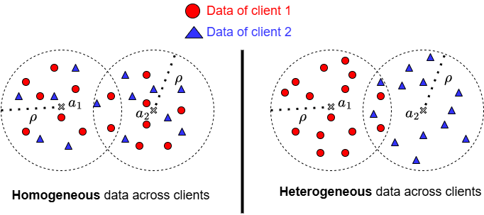
Figure 2: Illustration of (training) data generation for an example D-SVM problem with $K=2$ clients.

For convenience, we start with $K=2$. Consider an instance of the system of Figure 1 used for distributed binary classification with two clients. In this case, $\mathcal{Z}_{1}=\mathcal{X}_{1}\times\mathcal{Y}$ and $\mathcal{Z}_{2}=\mathcal{X}_{2}\times\mathcal{Y}$, with $\mathcal{Y}=\{-1,+1\}$. In accordance with the general setup of Section II, Client 1 has $n$ training samples $S_{1}=(Z_{1,1},\ldots,Z_{1,n})$ and Client 2 has $n$ training samples $S_{2}=(Z_{2,1},\ldots,Z_{2,n})$. Both clients use Support Vector Machines (SVM) to obtain respective models $W_{1}$ and $W_{2}$; and the aggregated model is $\overline{W}{=}(W_{1}+W_{2})/2$.

We investigate the question of the effect of the data heterogeneity across the two clients on the generalization error of the model $\overline{W}$. To this end, we compare the performance of $\overline{W}$ (from a generalization error perspective) in the following two settings, depicted pictorially in Figure 2.

• Heterogeneous data setting: In this case, for $k=1,2$ the training samples $\{(X_{k,j},Y_{k,j})\}_{j=1}^{n}$ of Client $k$ are drawn independently at random from an arbitrary distribution $\mu_{k}^{\text{Het}}$ which satisfies

  $$\mathbb{P}\big{(}\parallel X_{k,j}-a_{k}\parallel\leq\rho\big{)}=1,\quad\forall\>j\in[n].$$ (26)

  For example, the data of Client 1 drawn independently at random from uniform distribution over a $d$-dimensional ball with center $a_{1}$ and radius $\rho$, for some $a_{1}\in\mathbb{R}^{d}$ and $\rho\in\mathbb{R}^{+}$; and, similarly, the training samples of Client 2 drawn independently at random from the uniform distribution over a $d$-dimensional ball with center $a_{2}$ and radius $\rho$. That is, $X_{k,j}\sim\text{Unif}(\mathcal{B}(a_{k},\rho))$.

• Homogeneous data setting: In this case, both clients have their training samples picked independently at random from the same distribution $\mu^{\text{Hom}}=(\mu_{1}^{\text{Het}}+\mu_{2}^{\text{Het}})/2$. In particular, $\mu^{\text{Hom}}$ satisfies, for $k=1,2$ and every $j\in[n]$,

  $$\mathbb{P}\Big{(}\parallel X_{k,j}-a_{1}\parallel\leq\rho\>\>\text{or}\>\>\parallel X_{k,j}-a_{2}\parallel\leq\rho\Big{)}=1.$$ (27)

For both settings, we measure the generalization error as given by (6). For (5), we use the $0$-$1$ loss function $\ell_{0}(z,w)=\mathbbm{1}_{\big{\{}yf(x,w)<0\big{\}}}$, where the sign of $f(x,w)$ is the label prediction by hypothesis $w$ and $\mathbbm{1}$ is the indicator function, for the evaluation of the population risk; and, as it is common in related literature [25], we use the $0$-$1$ loss function with margin $\theta$, for some $\theta\in\mathbb{R}^{+}$, defined as $\ell_{\theta}(z,w)=\mathbbm{1}_{\big{\{}yf(x,w)<\theta\big{\}}}$, for the evaluation of the empirical risk. That is,

$$\operatorname{gen}_{\theta}(\overline{w})=\mathcal{L}(\overline{w})-\hat{\mathcal{L}}_{\theta}(S,\overline{w}).$$ (28)

V-A Heterogeneous and homogeneous data settings

The next theorem states bounds on the expected generalization error of the distributed SVM classification problem with $K=2$ clients for both heterogeneous and homogeneous data settings.

Theorem 7.

Let $\theta\in(0,1]$. The expected margin generalization error $\mathbb{E}[\text{gen}_{\theta}(S_{[K]},\overline{W})]$ is bounded by

$$\mathcal{O}\left(\sqrt{\frac{(\frac{\rho}{\theta})^{2}\log\left([3,\frac{\theta}{\rho}]^{+}\right)\log n+\frac{1}{2}\log\left(\frac{n^{2}\parallel a_{1}\parallel\parallel a_{2}\parallel}{\theta^{2}}\right)}{n}}\right).$$

in the heterogeneous data setting (26); and by

$$\mathcal{O}\left(\sqrt{\frac{\left(\frac{\rho^{\prime}}{\theta}\right)^{2}\log\left([3,\frac{\theta}{\rho^{\prime}}]^{+}\right)\log n+\log\left(\frac{n\parallel a^{\prime}\parallel}{\theta}\right)}{n}}\right),$$

with $\rho^{\prime}={\rho+\parallel a_{1}-a_{2}\parallel}$ and $a^{\prime}=\frac{(a_{1}+a_{2})}{2}$ in the homogeneous data setting (27).

Theorem 7 is a special case of a more general one that will follow, Theorem 8; and, for this reason, we state it without proof here.

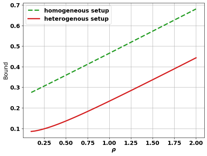
Figure 3: Evolution of the generalization bounds of Theorem 7 as function of ball radius $\rho$, for both heterogeneous and homogeneous data settings. System parameters are set to $n=1000$, $\theta=0.4$, $a_{1}=(0.1,\mathbf{0}_{d-1})$ and $a_{2}=(1.2,\mathbf{0}_{d-1})$.

V-B Comparison

We compare the bounds of Theorem 7. Note that this comparison amounts at selecting which training procedure among Option 1 (the $n$ training samples of Client 1 drawn according to $\mu_{1}^{\text{Het}}$ and those of Client 2 drawn according to $\mu_{2}^{\text{Het}}$) or Option 2 (both clients have their $n$ samples drawn according to $\mu^{\text{Hom}}=(\mu_{1}^{\text{Het}}+\mu_{2}^{\text{Het}})/2$) yield an aggregated model $\overline{W}=(W_{1}+W_{2})/2$ that generalizes better during test time. It is important to note that this comparison is fair, since the test samples are actually generated according to the same distribution in both settings, which is $\mu^{\text{Hom}}=(\mu_{1}^{\text{Het}}+\mu_{2}^{\text{Het}})/2$. This is easy to see as, for every $\overline{w}$ we have

$$\mathbb{E}_{Z_{1}\sim\mu^{\text{Het}}_{1}}[\ell(Z_{1},\overline{w})] +\mathbb{E}_{Z_{2}\sim\mu^{\text{Het}}_{2}}[\ell(Z_{2},\overline{w})]$$

$$=2\mathbb{E}_{Z\sim\mu^{\text{Hom}}}[\ell(Z,\overline{w})].$$ (29)

Figure 3 depicts the evolution of the bounds of Theorem 7 as function of the ball radius $\rho$, for both heterogeneous and homogeneous data settings (across clients). Note that, for fixed values of $n,a_{1},a_{2},\theta$, increasing $\rho$ is equivalent to diminishing the Total Variation distance between the distributions induced by (26) and (27). In fact, for large values of $\rho$ the volume of the intersection of the two balls is big; and this augments the probability of the two clients picking ‘similar’ samples. It is observed that the bound for the heterogeneous data setting is tighter (i.e., is smaller) than that for the associated homogeneous data setting. This suggests that, for this example, D-SVM generalizes better when the training data is heterogeneous across clients.

Finally, for both heterogeneous and homogeneous data settings, the bounds increase with $\rho$. This is somewhat expected as the ball volume increases with $\rho$, making it less likely for the generated training samples per-client (whose number $(n)$ is fixed) to be ‘representatives’ of all possible sample realizations over the ball during test time.

VI Effect of data heterogeneity on generalization for D-SVM: General case

In Section V we considered a distributed SVM setting with two extreme data-heterogeneity setups across two clients: fully homogeneity or fully heterogeneity. In this section, we generalize the setting of Section V to arbitrary number of ; and, most importantly, with gradually increasing data-heterogeneity setups.

More formally, fix $M\in\mathbb{N}^{*}$ arbitrary data distributions $\nu_{1},\ldots,\nu_{M}$ over $\mathcal{Z}=\mathcal{X}\times\mathcal{Y}$. Denote the $X$-marginal of $\nu_{m}$, $m\in[M]$, as $\nu_{m,X}$.

In the study of the generalization error of SVM, it is common to assume that the data is bounded [25, 19]. Hence, we assume that there exists $a_{m}\in\mathbb{R}^{d}$, $m\in[M]$, and $\rho\in\mathbb{R}^{+}$, such that

$$\operatorname{supp}\left(\nu_{m,X}\right)\subseteq B(a_{m},\rho),\quad m\in[M],$$ (30)

where $B(a_{m},\rho)$ denotes the $d$-dimensional ball with the center $a_{m}$ and radius $\rho$. Alternatively, we have that

$$\mathbb{P}_{X\sim\nu_{m,X}}\left(\left\|X-a_{m}\right\|\leq\rho\right){=}\mathbb{P}_{X\sim\nu_{m,X}}\left(X\in B(a_{m},\rho)\right){=}1.$$

Now, we define a family of setups indexed by $r=1,\ldots,M$ with gradually decreasing levels of data-heterogeneity across $K\geq M$ clients. Specifically, for every $r\in[M]$ and every $k\in[K]$ let $c_{k}^{(r)}=(k\mod[M-r+1])+1$. For $r=1,\ldots,M$ the $r$-th Setup has the clients’ data distributions defined each over exactly $r$ balls, as a suitable mixture of $r$ measures from the aforementioned set of distributions $\{\nu_{1},\ldots,\nu_{M}\}$. In particular, this allows to investigate the effect of the clients picking their training samples from partially overlapping data distributions, with the amount of overlap controled by the value of $r$. Spefically:

$r$-th Setup: the data distribution $\mu_{k}^{(r)}$ of client $k$ is

$$\mu_{k}^{(r)}=\sum\nolimits_{m=c_{k}^{(r)}}^{c_{k}^{(r)}+r-1}\alpha_{k,m}^{(r)}\nu_{m},$$ (31)

where $\{\alpha_{k,m}^{(r)}\}$ are arbitrary non-negative coefficients chosen such that $\sum_{k\in[K]}\alpha_{k,m}^{(r)}=1/M$ for every $(r,m)\in[M]^{2}$, $\sum_{m=c^{(r)}_{k}}^{c^{(r)}_{k}+r-1}\alpha_{k,m}^{(r)}=1$ for every $(k,r)\in[K]\times[M]$, and $\alpha_{k,m}^{(r)}=\alpha_{k^{\prime},m}^{(r)}$ if $c_{k}^{(r)}=c_{k^{\prime}}^{(r)}$. It is easy to check that for every $r\in[M]$, the set $\left\{\alpha_{k,m}^{(r)}\right\}$ always exists.

Notice that with the data distribution defined as (31), in the $r$-th Setup Client $k$ picks its training samples from the union of exactly $r$ balls; namely, those whose indices are in the set $\{c_{k}^{(r)},\ldots,c_{k}^{(r)}+r-1\}$. That is,

$$\mathbb{P}_{X_{k}\sim\mu_{k,X}^{(r)}}\left(X_{k}\in\bigcup\nolimits_{m=c_{k}^{(r)}}^{c_{k}^{(r)}+r-1}B(a_{m},\rho)\right)=1,$$

where $\mu_{k,X}^{(r)}$ stands for the $X_{k}$-marginal of $\mu_{k}^{(r)}$. In particular, this allows distinct clients picking their samples from partially overlapping set of balls. For example, the setup $r=M$ has all $K$ clients picking their training samples from the same distribution $\mu_{k}^{(M)}=\Big{(}\sum\nolimits_{m\in[M]}\nu_{m}\Big{)}/M$, i.e., the data is homogeneous across clients. As the value of $r$ decreases, the level of data heterogeneity across clients increases, reaching its maximum for $r=1$, a setup for which $M$ clients (among the $K$ participating ones) pick their samples from distinct distributions over distinct balls. In what follows, we will develop setup-dependent generalization bounds whose comparison will provide insights on the effect of data-heterogeneity on the generalization error of the studied D-SVM problem. It should be emphasized that, for the sake of fair comparison, the data distribution during “test” time is set to be identical for all clients and setups, given by $(\nu_{1}+\ldots+\nu_{M})/M$. This follows since using (31) and substuting using $\sum_{k\in[K]}\alpha_{k,m}^{(r)}=1/M$ we get $\Big{(}\sum\nolimits_{k\in[K]}\mu_{k}^{(r)}\Big{)}/K=\Big{(}\sum\nolimits_{m\in[M]}\nu_{m}\Big{)}/M$.

VI-A Generalization bound for the $r$’th setup

Define, for $r\in[M]$,

$$D_{k,r}=\max_{(i,j)}\>\>\|a_{i}-a_{j}\|,$$ (32)

where the maximization is over all pairs $(i,j)\in[{c^{(r)}_{k}},{c^{(r)}_{k}+r-1}]^{2}$.

Theorem 8.

Let $\theta\in(0,1]$. Then, for the $r$’th setup defined by (31) the expected margin generalization error $\mathbb{E}[\operatorname{gen}_{\theta}(S_{[K]},\overline{W})]$ is upper bounded by

$$\mathcal{O}\left(\sqrt{\frac{\sum_{k=1}^{K}\left[\Big{(}\frac{\rho_{k}^{(r)}}{K\theta}\Big{)}^{2}\log(nK)\log\left(\bar{E}^{(r)}_{k}\right){+}{\log}\bigg{(}\tilde{E}^{(r)}_{k}\bigg{)}\right]}{nK}}\right)$$

where $\bar{E}^{(r)}_{k}{=}\left[3,\frac{K\theta}{\rho^{(r)}_{k}}\right]^{+}$ and $\tilde{E}^{(r)}_{k}=\left[1,\frac{4n\|b^{(r)}_{k}\|}{K\theta}\right]^{+}$, with

$$\rho_{k}^{(r)}{=}\rho+D_{k,r},\quad\quad b^{(r)}_{k}{=}{\sum\nolimits_{m=c_{k}^{(r)}}^{c_{k}^{(r)}+r-1}\alpha^{(r)}_{k,m}a_{m}}.$$

This Theorem is proved in Appendix IX-G.

We pause to discuss the result of Theorem 8. First, note that for every setup $r=1,\ldots,M$ the contribution of Client $k$ to the bound is, up-to an additive logarithm term, proportional to the squared radius of the smallest ball that contains the union of the $r$ balls from which this client picks its training sample, i.e., $\rho_{k}^{(r)}{=}\rho+D_{k,r}$. Interestingly, shifts of these balls (through the values of $(a_{1},\ldots,a_{m})$ only changes marginally the value of the bound. This is in accordnace with the intuition that the classification error of a cloud of points should depend primarily on the relative spatial repartition of data points of distinct labels with respect to each other, rather than the distance to origin of the entire cloud. Second, the bound depends essentially on $(r,K,M)$ as well as the parameters of the data support for every client, i.e., the values of $\{\rho^{(r)}_{1},\ldots,\rho^{(r)}_{K}\}$.

Now, we discuss few special cases and the relation to some known prior art bounds. For $K=M=2$ setting $r=1$ one recovers the first bound of Theorem 7 and setting $r=2$ one recovers the second bound therein. For $M=1$ and $r=1$ Theorem 8 reduces to a bound of order

$$\mathcal{O}\Bigg{(}\sqrt{\frac{\rho^{2}\log(nK)\log\big{(}\bar{E}\big{)}+K^{2}\theta^{2}{\log}\Big{(}\tilde{E}\Big{)}}{nK^{2}\theta^{2}}}\Bigg{)},$$ (33)

with $\bar{E}=\left[\frac{K\theta}{\rho},3\right]^{+}\quad\text{and}\quad\tilde{E}=\left[1,\frac{4n\|a_{1}\|}{K\theta}\right]^{+}$, which is better than a previously established bound by [19, Theorem 5] which is of order

$$\mathcal{O}\Bigg{(}\sqrt{\frac{(\rho+\|a_{1}\|)^{2}\log(nK){\log}\Big{(}\Big{[}\frac{K\theta}{\rho+\|a_{1}\|},3\Big{]}^{+}\Big{)}}{nK^{2}\theta^{2}}}\Bigg{)}.$$ (34)

VI-B Improved generalization bound for DVSM in terms of Jensen-Shannon divergence

The following theorem, whose proof appears in Appendix IX-H, provides a possibly better bound in terms of the Jensen-Shannon divergence as captured by $h_{D}(\cdot,\cdot)$.

Theorem 9.

Let $\theta\in(0,1]$. Then, for the $r$’th setup defined by (31) the expected margin generalization error $\mathbb{E}[\operatorname{gen}_{\theta}(S_{[K]},\overline{W})]$ is upper bounded by

$$\mathcal{O}\left(h^{-1}_{D}\bigg{(}\hat{E}+\log(n)\Big{|}\mathbb{E}\left[\hat{\mathcal{L}}_{\theta}(S_{[K]},\overline{W})\right]-\frac{9}{nK\sqrt{K}}\bigg{)}-\mathbb{E}\left[\hat{\mathcal{L}}_{\theta}(S_{[K]},\overline{W})\right]+\frac{1}{nK\sqrt{K}}\right).$$ (35)

where

$$\hat{E}=\frac{1}{nK}\sum\limits_{k\in[K]}\left[\left(\frac{\rho^{(r)}_{k}}{K\theta}\right)^{2}\log(nK)\log\left(\bar{E}^{(r)}_{k}\right)+\log\left(\tilde{E}^{(r)}_{k}\right)\right],$$

with $\bar{E}^{(r)}_{k}$ and $\tilde{E}^{(r)}_{k}$ which defined as in Theorem 8

Using this result and Lemma 1, it can be easily seen that if the empirical risk is negligible then the expected margin generalization error is upper bounded by $\mathcal{O}\left(\frac{\log(K)\log(nK)}{nK^{2}}+\frac{\log(n)}{n}\right).$

VI-C An example with unbounded data support

So far we have analyzed SVM algorithms when applied to data with bounded support. In this section, we extend the result of Theorem 8 to an example data with un-bounded support. Fix $M\in\mathbb{N}^{\ast}$ and consider the data distributions $\nu_{1},\cdots,\nu_{M}$ such that if $X\sim\nu_{m}$ then $\|x-a_{m}\|$ has Gaussian distribution with zero-mean and variance $\sigma^{2}$. That is, the probability density function (PDF) of $X$ is given by

$$f_{X}(x)=\frac{1}{S_{m}^{d-1}\left(\|x-a_{m}\|\right)}\left(\frac{e^{-\frac{\|x-a_{m}\|^{2}}{2\sigma^{2}}}}{\sqrt{2\pi\sigma^{2}}}\right),$$ (36)

where $(x,a_{m})\in\mathbb{R}^{2d}$, $\sigma^{2}\in\mathbb{R}^{+}$ and, for $r\in\mathbb{R}^{+}$, $S_{m}^{d-1}(r)$ is the surface of a sphere in $\mathbb{R}^{d}$ with radius $r$, i.e.,

$$S_{m}^{d-1}(r)=\frac{2\pi^{\frac{d}{2}}r^{d-1}}{\Gamma\left(\frac{d}{2}\right)}.$$ (37)

Similar to in the previous section, we consider a hierarchy of setups with increasing degree of heterogeneity. Speficially, for the $r$-th setup the distribution of the data observed by the $k$-th client is given by

$$\mu^{(r)}_{k}=\sum\nolimits_{m=c^{(r)}_{k}}^{c^{(r)}_{k}+r-1}\alpha^{(r)}_{k,m}\nu_{m},$$ (38)

where the coefficients $\{\alpha_{k,m}^{(r)}\in\mathbb{R}^{+}\}$ are chosen such that $\sum_{k\in[K]}\alpha_{k,m}^{(r)}=1/M$ for every $(r,m)\in[M]^{2}$ and $\sum_{m=c^{(r)}_{k}}^{c^{(r)}_{k}+r-1}\alpha_{k,m}^{(r)}=1$ for every $(k,r)\in[K]\times[M]$. Also, $\alpha_{k,m}^{(r)}=\alpha_{k^{\prime},m}^{(r)}$ if $c_{k}^{(r)}=c_{k^{\prime}}^{(r)}$.

Theorem 10.

Let $\theta\in(0,1]$. Then, the expected margin generalization error $\mathbb{E}\left[\operatorname{gen}_{\theta}(S_{[K]},\overline{W})\right]$ in the $r$-th setup is upper bounded by

$$\mathcal{O}\left(\sqrt{\frac{\sum_{k=1}^{K}\left[\left(\frac{\rho^{(r)}_{k}}{K\theta}\right)^{2}\log\left(\bar{E}^{(r)}_{k}\right)\log(nK)+\log\left(\tilde{E}_{k}^{(r)}\right)\right]}{nK}}\right),$$ (39)

where $\rho_{k}^{(r)}=D_{k,r}+\sigma\sqrt{\log(nK)}$, $\bar{E}^{(r)}_{k}=\left[3,\frac{K\theta}{\sigma}\right]^{+}$ and $\tilde{E}_{k}^{(r)}=\left[1,\frac{4n\parallel b^{(r)}_{k}\parallel}{K\theta}\right]^{+}$, with $D_{k,r}$ defined as in (32) and $b^{(r)}_{k}{=}{\sum\nolimits_{m=c_{k}^{(r)}}^{c_{k}^{(r)}+r-1}\alpha^{(r)}_{k,m}a_{m}}$.

The proof of Theorem 10 is given in Appendix IX-I.

VI-D Comparison

A particularly interesting special case is when the balls are equally spaced, say by some $\Delta\in\mathbb{R}^{+}$, i.e., $\|a_{m}-a_{m-1}\|=\Delta$ for every $m\in[2:M]$. For simplicity, let $a_{1}=\mathbf{0}_{d}$. In this case, it is easy to see that the bound of Theorem 8 reduces to

$$\mathcal{O}\left(\sqrt{\frac{\bar{A}(K,r,\theta)\log(nK)}{nK^{2}\theta^{2}}{+}\frac{1}{n}\log\left(\tilde{A}(M,K,r,\Delta)\right)}\right),$$ (40)

where $\tilde{A}(M,K,r,\Delta)=\left[1,\frac{n\Delta(2M+r-1)}{K\theta}\right]^{+}$ and

$$\bar{A}(K,r,\theta){=}\Big{(}\rho{+}(r-1)\Delta\Big{)}^{2}\log\left(\left[3,\frac{K\theta}{\rho+(r-1)\Delta}\right]^{+}\right).$$

Similarly, in this case the bound of Theorem 10 reduces to

$$\mathcal{O}\left(\sqrt{\frac{\bar{B}(K,r,\theta)\log(nK)}{nK^{2}\theta^{2}}{+}\frac{1}{n}\log\left(\tilde{B}(M,K,r,\Delta)\right)}\right),$$ (41)

where $\tilde{B}(M,K,r,\Delta)=\left[1,\frac{n\Delta(2M+r-1)}{K\theta}\right]^{+}$ and

$$\bar{B}(K,r,\theta){=}\left({{{D_{k,r}}}+\sigma\sqrt{\log(nK)}}\right)^{2}\log\left(\left[3,\frac{K\theta}{\sigma}\right]^{+}\right).$$

Figure 4 depicts the evolution of the bound (40) versus $\rho$ for various values of $r=1,\ldots,M$, for an example D-SVM setting with $K=10$, $M=6$, $n=1000$, $\theta=1$ and $\Delta=1.0$. As it is visible from the figure the bound on the expected generalization is better (i.e., smaller) for smaller values of $r$, indicating that the aggregated model $\overline{W}=(W_{1}+\ldots+W_{K})/K$ generalizes better as the degree of training data heterogeneity across clients is bigger. Figure 5 shows similar results for the bound (41) whose evolution is depicted as a function of $\sigma$ for the same setting. For the special case $K=2$ the margin generalization bound derived of Theorem 10 reduces to

$$\mathcal{O}\left(\sqrt{\frac{\tilde{E}\log\left([3,\frac{\theta}{\sigma}]^{+}\right)\log n+\frac{1}{2}\log\left(\frac{n^{2}\parallel a_{1}\parallel\parallel a_{2}\parallel}{\theta^{2}}\right)}{n}}\right)$$ (42)

for the heterogeneous data setting (i.e., $r=1$); and to

$$\mathcal{O}\left(\sqrt{\frac{\bar{E}\log\left([3,\frac{\theta}{\sigma}]^{+}\right)\log n+\log\left(\frac{n\|a^{\prime}\|}{\theta}\right)}{n}}\right)$$ (43)

for the homogeneous data setting (i.e., $r=2$), where $\tilde{E}=\left(\frac{\sigma\sqrt{\log n}}{\theta}\right)^{2}$, $\bar{E}=\left(\frac{{{\|a_{1}-a_{2}\|}}+\sigma\sqrt{\log n}}{\theta}\right)^{2}$ and $a^{\prime}=\frac{(a_{1}+a_{2})}{2}$. These bounds (42) and (43) are compared in Figure  6, from which it can be seen that the result of Theorem 10 is tighter in smaller (i.e., better) in the across-clients heterogeneous data setting.

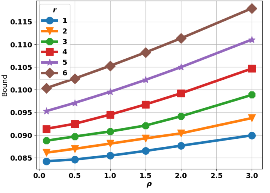
Figure 4: Evolution of the generalization bound (40) for various degrees of data heterogeneity across clients.

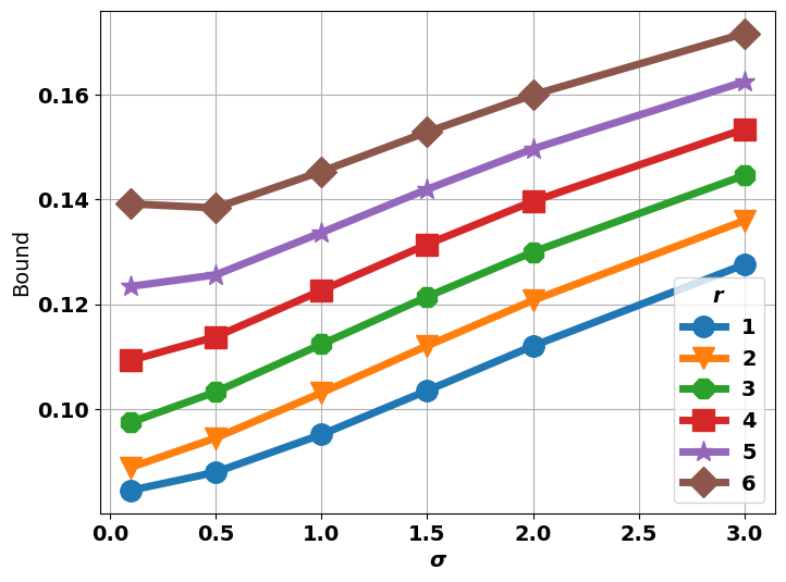
Figure 5: Evolution of the generalization bound (41) for various degrees of data heterogeneity across clients.

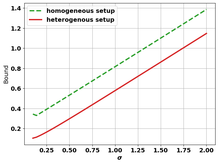
Figure 6: Evolution of the generalization bounds derived in (42) and (43) as function of parameter $\sigma$, for both heterogeneous and homogeneous data settings. System parameters are set to $n=1000$, $\theta=0.4$, $a_{1}=(0.1,\mathbf{0}_{d-1})$ and $a_{2}=(1.2,\mathbf{0}_{d-1})$.

VI-E Discussion

The aforementioned results advocate in favor of data heterogeneity across clients during training phase, in the sense that this provably helps for a better generalization. However, caution should be exercised in the interpretation of such finding as for the effect of data heterogeneity on the population risk. In particular, while there are reasons to believe that there might indeed exist cases in which heterogeneity helps also for a better (i.e., smaller) population risk (such as for realizable setups for which generalization error equals population risk), we make no such claim in general. This is because the positive decrease of the generalization error enabled by data heterogeneity may not compensate the caused increase of the empirical risk, causing the population risk to be larger - see Fig. 8 which shows the empirical and population risks for Experiment 1 that will follow.

VII Experimental results

We report the results of three experiments, all pertaining to D-SVM i.e., a distributed learning setup where each client trains a SVM model, but with different datasets and feature and/or label heterogeneity. Full details of all experiments are given in Appendix VIII.

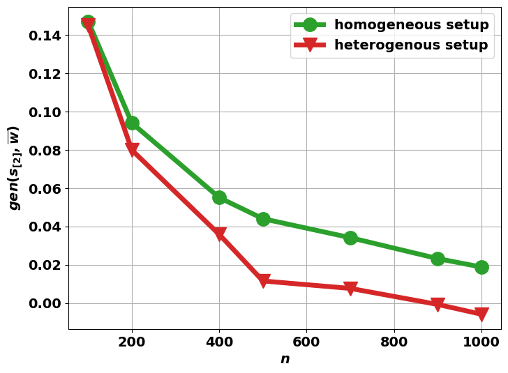
Figure 7: Measured generalization error for Experiment 1.

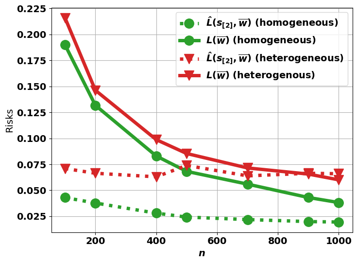
Figure 8: Empirical and population risks for Experiment 1.

Experiment 1 (Synthetic data with feature heterogeneity across clients): In this experiment, we consider binary classification using D-SVM with synthetic data in dimension $d=100$, generated as described in Section V. Figure 7 shows the evolution of the generalization error for the homogeneous and heterogeneous setups of Section V as a function of $n$. The reported values are averaged over 100 independent runs, where every client trains its local model in 300 epochs prior to aggregation. As it can be seen, for all values of $n$ the across-clients heterogeneous training data procedure yields a better (i.e., smaller) generalization error than the associated across-clients homogeneous training data procedure.

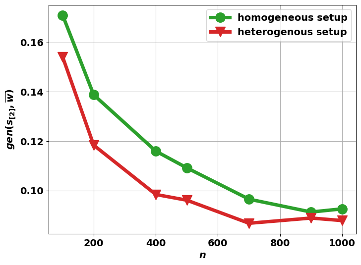
Figure 9: Measured generalization error for Experiment 2.

Experiment 2 (MNIST data with feature heterogeneity across clients): In this experiment, we consider binary classification with two classes (here 1 and 6) of the MNIST dataset [26]. To introduce feature heterogeneity, we add Gaussian white noise with standard deviation $\sigma=0.2$ to half of the training MNIST images. Then, two setups are compared. In the heteregeneous data setup, Client 1 possesses all the noisy data while the second one has only non-noisy original images. In the homogeneous setup, every client picks its data uniformly at random from noisy and non-noisy digits, thus resulting in half of its training samples noisy and the other half non-noisy. Figure 9 shows the evolution of the generalization error (evaluated as described in Section V) for both homogeneous and heterogeneous setups. The reported values are averaged over 100 independent runs, each performed using 200 local SGD epochs prior to aggregation. Here too, as it is visible from the figure feature-heterogeneity helps for a better, i.e., smaller, generalization error.

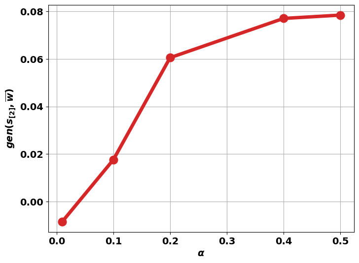
Figure 10: Measured generalization error for Experiment 3, as function of the degree $(\alpha)$ of label heterogeneity across clients - smaller $\alpha$ corresponds to bigger heterogeneity.

Experiment 3: (MNIST data with label heterogeneity across clients): In this experiment, we consider binary classification of two digits (6 and 9) of the MNIST dataset. The training samples are split equally among the two clients, but in a manner that creates some label-heterogeneity among them. Specifically, Client 1 is assigned a proportion $\alpha$ of the entire training digits 6 and a proportion $(1-\alpha)$ of the training digits 9. Client 2 has the remaining training digits, i.e., proportion $(1-\alpha)$ of the digits 6 and $\alpha$ of the digits 9. As it is visible from Figure 10, bigger degrees of heterogeneity (i.e., smaller $\alpha\in[0,1/2]$) yield smaller generalization error. It is worth noting that this experiment, which somewhat stretches our problem setup, also indicates that the observations and insights of this paper (on the effect of data heterogeneity across clients on generalization error) may hold more generally, beyond the setup of Section V.

Appendices

The appendices are organized as follows:

• Appendix VIII contains the details of the experiments presented in Section VII.

• Appendix IX contains all the proofs of the results of the papers, in the order of their appearance, that is:

  • Proof of Theorem 1 presented in Appendix IX-A,

  • Proof of Theorem 2 presented in Appendix IX-B,

  • Proof of Theorem 3 presented in Appendix IX-C,

  • Proof of Theorem 4 presented in Appendix IX-D,

  • Proof of Theorem 5 presented in Appendix IX-E,

  • Proof of Theorem 6 presented in Appendix IX-F,

  • Proof of Theorem 8 presented in Appendix IX-G,

  • Proof of Theorem 9 presented in Appendix IX-H,

  • Proof of Theorem 10 presented in Appendix IX-I

  • Proof of Lemma 1 presented in Appendix IX-J,

  • Proof of Lemma 2 presented in Appendix IX-K.

VIII Details of experimental results

VIII-A Experiment 1

For the first experiments, we use synthetic data, generated as explained in Section VII of the paper. The data dimension is $d=100$. The two balls have the following characteristics.

• Ball 1:

  • Center: $a_{1}=(-2,0,\ldots,0)^{\top}$

  • Radius: $\rho=2.0$

  • Labels: $y=\mathbbm{1}_{w^{T}x+a_{1}/5>0}$, where $w=(-0.2,1,\ldots,1)$

• Ball 2:

  • Center: $a_{2}=(2,0,\ldots,0)^{\top}$

  • Radius: $\rho=2.0$

  • Labels: $y=\mathbbm{1}_{w^{T}x+a_{2}/5>0}$, where $w=(-0.2,1,\ldots,1)$

See Fig. 11 for an illustration of the synthetic data for dimension $d=2$.

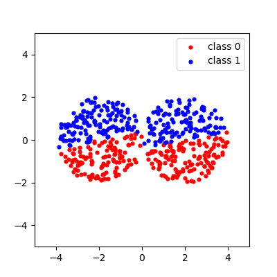
Figure 11: Synthetic data for Experiment 1, $d=2$

To illustrate our theoretical results, in particular the generalization bounds of Theorem 4 and 5, the two clients train a SVM model. They each perform 300 epochs using SGD with learning rate 0.005. Moreover, the whole setup has been run 300 times to account for the overall randomness and estimate the expectation in the bounds of Theorems 4 and 5.

VIII-B Experiment 2

The data used for the second experiment is two classes extracted from the MNIST dataset (1 and 6). The images were normalized and projected into a space of dimension $d=2000$ using a Gaussian kernel with scale parameter $\gamma=0.01$. Then, AWGN with standard deviation $\sigma=0.2$ was added to the images. We still consider a two client distributed setup, where each client trains a SVM model using SGD with learning rate 0.01. 200 epochs were run and the simulations were performed and simulations were performed 100 times.

VIII-C Experiment 3

In this last experiment, beyond the setup considered for the theoretical results of our paper, we use real-world data i.e., the MNIST dataset. We extract two classes out of it (6 and 9) in order to perform binary classification. The only preprocessing that has been performed is normalization of the images.

Unlike in the previous experiments, each client here trains a convolutional neural network with two convolutional layers, a dropout layer and two fully-connected layers. We minimize the binary cross-entropy loss, using mini-batch SGD with batch size 64 and learning rate 0.01. 300 communication rounds were run and simulations were performed 10 times.

VIII-D Implemental and hardware details

All experiments were done using Python 3.12.7 on a machine with the following specifications:

• CPU: AMD Ryzen 7 5800X (8 cores)

• GPU: Nvidia Geforce RTX 3070

• RAM: 32 GB

SVM models and were implemented using the Scikit-learn library. In particular, we used “RBFSampler” for kernel projection. CNN models were implemented using the Pytorch library.

IX Proofs

IX-A Proof of Theorem 1

Recall Definition 1. Also, recall the definition of the membership vectors $\mathbf{J}_{k}$ and $\mathbf{J}^{c}_{k}$ as given in the beginning of Section III. Let, for $k\in[K]$, $\mathcal{Q}_{k}$ be the set of type-I symmetric priors on $W_{k}$ conditionnally given $(S_{k},S^{\prime}_{k})$. The proof consists of two steps: In the first step, we prove that

$$\inf_{{Q}_{k}\in\mathcal{Q}_{k}}\mathbb{E}_{S_{k},S^{\prime}_{k}}\left[D_{KL}\left(P_{W_{k}|S_{k},S^{\prime}_{k}}\parallel Q_{k}\right)\right]=I\left(W_{k};\mathbf{J}_{k}|\mathfrak{Z}_{k}^{2n}\right).$$ (44)

In the second step, we show that for every $(Q_{1},\ldots,Q_{K})\in\mathcal{Q}_{1}\times\ldots\times\mathcal{Q}_{K}$ it holds that

$$\mathbb{E}_{S_{[K]},\overline{W}}\left[\operatorname{gen}(S_{[K]},\overline{W})\right]\leq\sqrt{\frac{2E}{n}},$$ (45)

where

$$E =\frac{1}{K}\sum_{k=1}^{K}\mathbb{E}_{S_{k},S_{k}^{\prime}}\left[D_{KL}\left(P_{W_{k}\mid S_{k},S_{k}^{\prime}}\parallel{Q}_{k}\right)\right].$$ (46)

In order to show the first step, consider the set $\mathcal{Q}_{k}^{\prime}$ of all conditional priors ${Q}_{k}^{\prime}$ that can be expressed as

$$Q_{k}^{\prime}\left(W_{k}|S_{k},S_{k}^{\prime}\right)=\mathbb{E}_{\mathbf{J}_{k}}\left[Q_{k,1}^{\prime}\left(W_{k}|\mathfrak{Z}^{2n}_{\mathbf{J}_{k}},\mathfrak{Z}^{2n}_{\mathbf{J}_{k}^{c}}\right)\right]$$ (47)

for some arbitrary conditional distribution $Q_{k,1}^{\prime}$. It is easy to verify that $\mathcal{Q}_{k}=\mathcal{Q}_{k}^{\prime}$. Therefore, we have

$$\inf_{{Q}_{k}\in\mathcal{Q}_{k}}\mathbb{E}_{S_{k},S^{\prime}_{k}}\left[D_{KL}\left(P_{W_{k}\mid S_{k},S^{\prime}_{k}}\parallel Q_{k}\right)\right]=\inf_{{Q}_{k}^{\prime}\in\mathcal{Q}_{k}^{\prime}}\mathbb{E}_{S_{k},S^{\prime}_{k}}\left[D_{KL}\left(P_{W_{k}\mid S_{k},S^{\prime}_{k}}\parallel Q_{k}^{\prime}\right)\right].$$ (48)

Recall that the vector $\mathfrak{Z}^{2n}_{k}$ is a re-arrangement of the elements of $(S_{k},S_{k}^{\prime})$, indexed by the vector $\mathbf{J}_{k}$. Using this, we get

$$\inf_{{Q}_{k}\in\mathcal{Q}_{k}}\mathbb{E}_{S_{k},S^{\prime}_{k}}\left[D_{KL}\left(P_{W_{k}\lvert S_{k},S^{\prime}_{k}}\parallel{Q}_{k}\right)\right] =\inf_{{{Q}}^{\prime}_{k}\in\mathcal{Q}^{\prime}_{k}}\mathbb{E}_{S_{k},S^{\prime}_{k}}\left[D_{KL}\left(P_{W_{k}\lvert S_{k},S^{\prime}_{k}}\parallel{Q}^{\prime}_{k}\right)\right]$$

$$=\inf_{{{Q}}^{\prime}_{k}\in\mathcal{Q}^{\prime}_{k}}\mathbb{E}_{\mathfrak{Z}_{k}^{2n}}\mathbb{E}_{\mathbf{J}_{k}}\left[D_{KL}\left(P_{W_{k}\lvert{\mathfrak{Z}^{2n}_{{\mathbf{J}}_{k}},{\mathfrak{Z}^{2n}_{\mathbf{J}_{k}^{c}}}}}\parallel{Q}^{\prime}_{k}\right)\right]$$

$$=\inf_{{Q}^{\prime}_{k,1}}\mathbb{E}_{\mathfrak{Z}_{k}^{2n}}\mathbb{E}_{\mathbf{J}_{k}}\left[D_{KL}\left(P_{W_{k}\lvert{\mathfrak{Z}^{2n}_{\mathbf{J}_{k}},{\mathfrak{Z}^{2n}_{\mathbf{J}_{k}^{c}}}}}\parallel\mathbb{E}_{\mathbf{J}_{k}}\left[{Q}^{\prime}_{k,1}\left(W_{k}\lvert\mathfrak{Z}^{2n}_{{\mathbf{J}}_{k}},\mathfrak{Z}^{2n}_{{\mathbf{J}}^{c}_{k}}\right)\right]\right)\right]$$

$$=I(W_{k};\mathbf{J}_{k}\lvert\mathfrak{Z}_{k}^{2n});$$ (49)

where the third equality follows using (47); and this completes the proof of the first step.

We now turn to the proof of the second step. By (6), for arbitrary $\lambda$ we have

$$\lambda\mathbb{E}_{S_{[K]},\overline{W}}\left[\operatorname{gen}\left(S_{[K]},\overline{W}\right)\right] =\frac{\lambda}{K}\sum_{k\in[K]}\mathbb{E}_{S_{k},\overline{W}}\left[\operatorname{gen}\left(S_{k},\overline{W}\right)\right]$$

$$=\frac{\lambda}{K}\sum_{k\in[K]}\mathbb{E}\left[\frac{1}{n}\sum_{i\in[n]}\bigg{(}\ell(z^{\prime}_{k,i},\overline{W})-\ell(z_{k,i},\overline{W})\bigg{)}\right]$$ (50)

$$\leq\sum_{k\in[K]}\frac{1}{K}\Bigg{(}D_{KL}\left({\mu}^{\otimes 2n}_{k}\otimes P_{\overline{W},W_{k}\lvert S_{k},S^{\prime}_{k}}\parallel{\mu}^{\otimes 2n}_{k}\otimes{Q}_{k}\otimes\overline{P}_{k}\right)$$

$$\hskip 71.13188pt+\log\mathbb{E}\left[e^{\frac{\lambda}{n}\sum_{i\in[n]}\left(\ell(z^{\prime}_{k,i},\overline{W})-\ell(z_{k,i},\overline{W})\right)}\right]\Bigg{)},$$ (51)

where:

• ${Q}_{k}\left(W_{k}|S_{k},S^{\prime}_{k}\right)$ and $P_{\overline{W}|W_{k},S^{\prime}_{k},S_{k}}$ are abbreviated as ${Q}_{k}$ and $\overline{P}_{k}$, respectively,

• the expectation in (50) and (51) is taken with respect to $(S_{k},S^{\prime}_{k},\overline{W},W_{k})$, with the joint distribution being $P_{S^{\prime}_{k}}\otimes P_{S_{k},\overline{W},W_{k}}$ for (50) and $\mu^{\otimes 2n}_{k}\otimes Q_{k}\otimes\overline{P}_{k}$ for (51),

• and (51) follows by application of Donsker-Varadhan’s variational representation, using that the loss is bounded and so sub-Gaussian.

Now, we proceed to upper bound the second term of the RHS of (51). Recall that for a membership vector $\mathbf{J}_{k}=\{J_{k,1},\cdots,J_{k,n}\}$ the vector $\mathfrak{Z}^{2n}_{\mathbf{J}_{k}}\in\mathcal{Z}^{2n}$ stands for the size-$n$ sub-vector of vector $\mathfrak{Z}^{2n}_{k}$ whose elements are indexed by $\mathbf{J}_{k}$. Thus, we have

$$\log\mathbb{E}\Big{[}e^{\frac{\lambda}{n}\sum_{i\in[n]}\left(\ell(z^{\prime}_{k,i},\overline{W})-\ell(z_{k,i},\overline{W})\right)}\Big{]} =\log\mathbb{E}\left[e^{\frac{\lambda}{n}\sum_{i\in[n]}\ell(\mathfrak{Z}_{J^{c}_{k,i}},\overline{W})-\ell(\mathfrak{Z}_{J_{k,i}},\overline{W})}\right]$$ (52)

$$=\log\mathbb{E}\left[\mathbb{E}_{\mathbf{J}_{k}\sim\text{Bern}\left(\frac{1}{2}\right)^{\otimes n}}\left[e^{\frac{\lambda}{n}\sum_{i\in[n]}\ell(\mathfrak{Z}_{J^{c}_{k,i}},\overline{W})-\ell(\mathfrak{Z}_{J_{k,i}},\overline{W})}\right]\right]$$ (53)

$$\leq\log\left(\frac{e^{\frac{\lambda}{n}}+e^{-\frac{\lambda}{n}}}{2}\right)^{n}$$ (54)

$$\leq\frac{\lambda^{2}}{2n},$$ (55)

where:

• the expectation in the LHS of (52) is taken over the random variables $(S_{k},S^{\prime}_{k},W_{k},\overline{W})$, distributed according to ${\mu}^{\otimes 2n}_{k}\otimes{Q}_{k}\left(W_{k}\lvert S_{k},S^{\prime}_{k}\right)\otimes P_{\overline{W}\lvert W_{k},S^{\prime}_{k},S_{k}}$.

• the expectation in the RHS of (52) is taken over the random variables $({\mathfrak{Z}}_{k}^{2n},W_{k},\overline{W},\mathbf{J}_{k})$, with the joint distribution given by $\mu^{\otimes 2n}_{k}\otimes{Q}_{k}(W_{k}\lvert{\mathfrak{Z}_{\mathbf{J}_{k}}^{2n}},\mathfrak{Z}_{\mathbf{J}^{c}_{k}}^{2n})\otimes P_{\overline{W}\lvert W_{k},\mathfrak{Z}_{\mathbf{J}_{k}}^{2n}}\otimes\text{Bern}\left(\frac{1}{2}\right)^{\otimes n}$.

• the expectation in (53) is taken over the random variables $({\mathfrak{Z}}_{k}^{2n},W_{k},\overline{W})$, with the joint distribution described by $\mu^{\otimes 2n}_{k}\otimes{Q}(W_{k}|\mathfrak{Z}_{k}^{2n})\otimes P(\overline{W}|W_{k},\mathfrak{Z}_{k}^{2n})$.

• the conditionals ${Q}_{k}(W_{k}|S_{k},S^{\prime}_{k})$ and $P_{\overline{W}\mid W_{k},S^{\prime}_{k},S_{k}}$ are both symmetric with respect to $S^{\prime}_{k},S_{k}$ – the symmetry of ${Q}_{k}(W_{k}|S_{k},S^{\prime}_{k})$ holds by assumption and that of $P_{\overline{W}\mid W_{k},S^{\prime}_{k},S_{k}}$ follows by use of Markov’s chain $\overline{W}-W_{k}-(S_{k},S^{\prime}_{k})$. This implies the symmetry over joint distribution of ${Q}_{k}(W_{k}|S_{k},S^{\prime}_{k})\otimes P_{\overline{W}\mid W_{k},S^{\prime}_{k},S_{k}}$ with respect to $(S_{k},S^{\prime}_{k})$; and, so, the RHS of (52) and that of (53) are identical.

• (54) follows by using the inequality

  $$\frac{e^{x}+e^{-x}}{2}\leq e^{\frac{x^{2}}{2}},$$ (56)

  and the fact that $\ell(z,w)\in[0,1]$ for all realization of $(z,w)\in(\mathcal{Z},\mathcal{W})$.

Continuing from (51) and substuting using (55) we get

$$\mathbb{E}_{S_{[K]},\overline{W}}\left[\operatorname{gen}(S_{[K]},\overline{W})\right]\leq\frac{1}{K\lambda}\sum_{k\in[K]}D_{KL}\left({\mu}^{\otimes 2n}_{k}\otimes P_{\overline{W},W_{k}\lvert S_{k},S^{\prime}_{k}}\parallel{\mu}^{\otimes 2n}_{k}\otimes{Q}_{k}\otimes\overline{P}_{k}\right)+\frac{\lambda}{2n}.$$ (57)

This inequality can be further simplified as:

$$\mathbb{E}_{S_{[K]},\overline{W}}\left[\operatorname{gen}(S_{[K]},\overline{W})\right] \leq\frac{1}{K\lambda}\sum_{k\in[K]}D_{KL}({\mu}^{\otimes 2n}_{k}\otimes P_{\overline{W},W_{k}\lvert S_{k},S^{\prime}_{k}}\parallel{\mu}^{\otimes 2n}_{k}\otimes{Q}_{k}\otimes\overline{P}_{k})+\frac{\lambda}{2n}$$ (58)

$$=\frac{1}{K\lambda}\sum_{k\in[K]}D_{KL}({\mu}^{\otimes 2n}_{k}\otimes P_{W_{k}\lvert S_{k},S^{\prime}_{k}}\otimes\overline{P}_{k}\parallel{\mu}^{\otimes 2n}_{k}\otimes{Q}_{k}\otimes\overline{P}_{k})+\frac{\lambda}{2n}$$ (59)

$$=\frac{1}{K\lambda}\sum_{k\in[K]}D_{KL}\left({\mu}^{\otimes 2n}_{k}\otimes P_{W_{k}\lvert S_{k},S^{\prime}_{k}}\parallel{\mu}^{\otimes 2n}_{k}\otimes{Q}_{k}\right)+\frac{\lambda}{2n}.$$ (60)

Finally, letting

$$\lambda =\sqrt{\frac{2n}{K}\sum_{k\in[K]}D_{KL}\left({\mu}^{\otimes 2n}_{k}\otimes P_{W_{k}|S_{k},S^{\prime}_{k}}\parallel{\mu}^{\otimes 2n}_{k}\otimes{Q}_{k}\right)}$$ (61)

$$=\sqrt{\frac{2n}{K}\sum_{k\in[K]}\mathbb{E}_{S_{k},S^{\prime}_{k}}\left[D_{KL}\left(P_{W_{k}|S_{k},S^{\prime}_{k}}\parallel{Q}_{k}\right)\right]},$$ (62)

and substuting in (60) completes the proof of the second step; and so that of the theorem.

IX-B Proof of Theorem 2

Let us consider the random variable $\Delta(S_{[K]},{Q}_{[K]})$ as

$$\Delta(S_{[K]},{Q}_{[K]})=\sqrt{\frac{\sum_{k\in[K]}\mathbb{E}_{S^{\prime}_{[K]}}\left[D_{KL}\left(P_{{W_{k}}\lvert S_{k},S^{\prime}_{k}}\parallel{Q}_{k}\right)\right]+K\log\left(\sqrt{2n}\right)+\log(1/\delta)}{K\lambda^{\ast}}},$$ (63)

and

$$\lambda^{\ast}=\frac{(2n-1)}{4}.$$

Then, we can write

$$\mathbb{P}\Big{(}\mathbb{E}_{P_{\overline{W},W_{k}\lvert S_{[K]}}} \left[\operatorname{gen}(S_{[K]},\overline{W})\right]>\Delta(S_{[K]},{Q}_{[K]})\Big{)}$$ (64)

$$\qquad=\mathbb{P}\Big{(}\frac{1}{K}\sum\limits_{k\in[K]}\mathbb{E}_{S^{\prime}_{k}}\mathbb{E}_{P_{\overline{W},W_{k}\lvert S_{k},S^{\prime}_{k}}}\left[\hat{\mathcal{L}}(S^{\prime}_{k},\overline{W})-\hat{\mathcal{L}}(S_{k},\overline{W})\right]>\Delta(S_{[K]},{Q}_{[K]})\Big{)}$$ (65)

$$\qquad\leq\mathbb{P}\Bigg{(}\bigg{(}\frac{1}{K}\sum\limits_{k\in[K]}\mathbb{E}_{S^{\prime}_{k}}\left[\mathbb{E}_{P_{\overline{W},W_{k}\lvert S^{\prime}_{k},S_{k}}}\left[\hat{\mathcal{L}}(S^{\prime}_{k},\overline{W})-\hat{\mathcal{L}}(S_{k},\overline{W})\right]\right]\bigg{)}^{2}>{\Delta^{2}(S_{[K]},{Q}_{[K]})}\Bigg{)}$$ (66)

$$\qquad\leq\mathbb{P}\Bigg{(}\frac{1}{K}\sum_{k\in[K]}\left(\mathbb{E}_{S^{\prime}_{k}}\mathbb{E}_{P_{\overline{W},W_{k}\lvert S^{\prime}_{k},S_{k}}}\left[\hat{\mathcal{L}}(S^{\prime}_{k},\overline{W})-\hat{\mathcal{L}}(S_{k},\overline{W})\right]\right)^{2}>\Delta^{2}(S_{[K]},{Q}_{[K]})\Bigg{)}$$ (67)

$$\qquad=\mathbb{P}\Bigg{(}\lambda^{\ast}\sum_{k\in[K]}\Bigg{(}\mathbb{E}_{S^{\prime}_{k}}\mathbb{E}_{P_{\overline{W},W_{k}\lvert S^{\prime}_{k},S_{k}}}\left[\hat{\mathcal{L}}(S^{\prime}_{k},\overline{W})-\hat{\mathcal{L}}(S_{k},\overline{W})\right]\Bigg{)}^{2}>{\lambda^{\ast}K{\Delta^{2}(S_{[K]},{Q}_{[K]})}}\Bigg{)}$$ (68)

$$\qquad\leq\mathbb{P}\Bigg{(}\lambda^{\ast}\sum_{k\in[K]}\mathbb{E}_{S^{\prime}_{k}}\mathbb{E}_{P_{\overline{W},W_{k}\lvert S^{\prime}_{k},S_{k}}}\left[\left(\hat{\mathcal{L}}(S^{\prime}_{k},\overline{W})-\hat{\mathcal{L}}(S_{k},\overline{W})\right)^{2}\right]>{\lambda^{\ast}K{\Delta^{2}(S_{[K]},{Q}_{[K]})}}\Bigg{)}$$ (69)

$$\qquad\leq\mathbb{P}\bigg{(}\sum\limits_{k\in[K]}\mathbb{E}_{S^{\prime}_{k}}\left(D_{KL}\left(P_{\overline{W},W_{k}\lvert S_{k},S^{\prime}_{k}}\parallel\overline{P}_{k}\otimes{Q}_{k}\right)\right)$$ (70)

$$\qquad\quad\quad+\sum\limits_{k\in[K]}\mathbb{E}_{S^{\prime}_{k}}\bigg{(}\log\mathbb{E}_{\overline{P}_{k}\otimes{Q}_{k}}\left[e^{\lambda^{\ast}\left(\hat{\mathcal{L}}(S^{\prime}_{k},\overline{W})-\hat{\mathcal{L}}(S_{k},\overline{W})\right)^{2}}\right]\bigg{)}\geq{\lambda^{\ast}K{\Delta^{2}(S_{[K]},{Q}_{[K]})}}\bigg{)}$$ (71)

$$\qquad\leq\mathbb{P}\bigg{(}\sum\limits_{k\in[K]}\mathbb{E}_{{\mu_{k}^{\otimes n}}}\left(\log\mathbb{E}_{\overline{P}_{k}\otimes{Q}_{k}}\left[e^{\lambda^{\ast}\left(\hat{\mathcal{L}}(S^{\prime}_{k},\overline{W})-\hat{\mathcal{L}}(S_{k},\overline{W})\right)^{2}}\right]\right)\geq$$ (72)

$$\quad\qquad\qquad\sum_{k\in[K]}\log\mathbb{E}_{\mu^{\otimes 2n}_{k}\otimes\overline{P}_{k}\otimes{Q}_{k}}\Big{[}e^{\lambda^{\ast}\left(\hat{\mathcal{L}}(S^{\prime}_{k},\overline{W})-\hat{\mathcal{L}}(S_{k},\overline{W})\right)^{2}}\Big{]}+\log(1/\delta)\bigg{)}$$ (73)

$$\qquad\leq\delta,$$ (74)

where

• $S_{[K]}$ is distributed as $S_{[K]}\sim\prod_{k=1}^{K}\mu^{\otimes n}_{k}$,

• the probability distributions $P_{\overline{W}|W_{k},S_{k},S^{\prime}_{k}}$ and ${Q}_{k}(\overline{W}|S_{k},S^{\prime}_{k})$ are denoted by $\overline{P}_{k}$ and ${Q}_{k}$, respectively, as before, and (69) are due to Jensen’s inequality for the convex function $f(x)=x^{2}$,

• equations (70-71) are concluded using the Donsker-Varadhan’s variational representation lemma,

• and Markov inequality yields the final inequality in (74).

It remains to show that

$$\sum_{k\in[K]}\log\mathbb{E}_{\mu^{\otimes 2n}_{k}\otimes\overline{P}_{k}\otimes{Q}_{k}}\Big{[}e^{\lambda^{\ast}\left(\hat{\mathcal{L}}(S^{\prime}_{k},\overline{W})-\hat{\mathcal{L}}(S_{k},\overline{W})\right)^{2}}\Big{]} \leq K\log(\sqrt{2n}),$$ (75)

where expectation is with respect to the probability distribution $\mu^{2n}_{k}\otimes\overline{P}_{k}\otimes{Q}_{k}$.

To show this, the left-hand side of (75) can be re-written as

$$\sum_{k\in[K]}\log\mathbb{E}_{\mu^{\otimes 2n}_{k}\otimes\overline{P}_{k}\otimes{Q}_{k}}\Big{[}e^{\lambda^{\ast}\left(\hat{\mathcal{L}}(S^{\prime}_{k},\overline{W})-\hat{\mathcal{L}}(S_{k},\overline{W})\right)^{2}}\Big{]} =\sum\limits_{k\in[K]}\log\mathbb{E}\Big{[}e^{\lambda^{\ast}\left(\frac{1}{n}\sum_{i\in[n]}\left[\ell(Z^{\prime}_{k,i},\overline{W})-\ell(Z_{k,i},\overline{W})\right]\right)^{2}}\Big{]}$$ (76)

$$=\sum\limits_{k\in[K]}\log\mathbb{E}\left[e^{\lambda^{\ast}\left(\frac{1}{n}\sum_{i\in[n]}\left[\ell(\mathfrak{Z}_{J_{k,i}},\overline{W})-\ell(\mathfrak{Z}_{J^{c}_{k,i}},\overline{W})\right]\right)^{2}}\right]$$ (77)

$$=\sum\limits_{k\in[K]}\log\mathbb{E}\Bigg{[}\mathbb{E}_{\mathbf{J}_{k}}\left[e^{\lambda^{\ast}\left(\frac{1}{n}\sum_{i\in[n]}\left(\ell\left[\mathfrak{Z}_{J_{k,i}},\overline{W})-\ell(\mathfrak{Z}_{J^{c}_{k,i}},\overline{W}\right]\right)\right)^{2}}\right]\Bigg{]}$$ (78)

$$\leq K\log(\sqrt{2n}),$$ (79)

where

• the expectation in the right-hand side of (76) is with respect to the probability distribution ${\mu^{2n}_{k}\otimes\overline{P}_{k}\otimes{Q}_{k}}$,

• the expectation in (77) is with respect to ${\mu^{\otimes 2n}_{k}\otimes P_{\overline{W}\lvert W_{k},\mathfrak{Z}_{k}^{2n}}\otimes{Q}_{k}({W_{k}}\lvert\mathfrak{Z}_{k}^{2n})\otimes\text{Bern}\left(\frac{1}{2}\right)^{\otimes n}}$,

• equation (78) uses ${\mu^{\otimes 2n}_{k}\otimes{Q}_{k}({W_{k}}\lvert\mathfrak{Z}_{k}^{2n})\otimes P_{\overline{W}\lvert W_{k},\mathfrak{Z}_{k}^{2n}}}$ as join distribution for computing the expectation,

• the equation (77) follows from the symmetry of $P_{\overline{W}\mid W_{k},S_{k},S^{\prime}_{k}}\otimes Q_{k}(\overline{W}|S_{k},S^{\prime}_{k})$ with respect to $(S_{k},S^{\prime}_{k})$. The symmetry in $P_{\overline{W}|W_{k},S_{k},S^{\prime}_{k}}$ arises from the Markov chain $\overline{W}-W_{k}-(S_{k},S^{\prime}_{k})$ in $P_{\overline{W}|W_{k},S_{k},S^{\prime}_{k}}$, and the symmetry in $Q_{k}(\overline{W}|S_{k},S^{\prime}_{k})$ follows from the assumptions. These two separate symmetric properties together imply the symmetry of $P_{\overline{W}|W_{k},S_{k},S^{\prime}_{k}}\otimes Q_{k}(\overline{W}\mid S_{k},S^{\prime}_{k})$.

• the expecationf in equation (78) is computed with respect to random variable $\mathbf{J}_{k}\sim\text{Bern}\left(\frac{1}{2}\right)^{\otimes n}$

• the equation (79) is concluded since

  $$\frac{1}{n}\sum_{i\in[n]}\left[\ell\left(\mathfrak{Z}_{J_{k,i}},\overline{W})-\ell(\mathfrak{Z}_{J^{c}_{k,i}},\overline{W}\right)\right],$$

  is $1/\sqrt{n}$-subgaussian for any $k\in[K]$ and hence

  $$\mathbb{E}_{\mathbf{J}_{k}\sim\text{Bern}\left(\frac{1}{2}\right)^{\otimes n}}\left[e^{\frac{\left[\frac{1}{n}\sum_{i\in[n]}\left(\ell(\mathfrak{Z}_{J_{k,i}},\overline{W})-\ell(\mathfrak{Z}_{J^{c}_{k,i}},\overline{W})\right)\right]^{2}}{(4/2n-1)}}\right]\leq\sqrt{2n},$$

where concluded from [27, Theorem 2.6.VI] and this completes the proof.

IX-C Proof of Theorem 3

We have

$$\mathbb{E}\left[\operatorname{gen}(S_{[K]},\overline{W})\right] =\frac{1}{K}\sum_{k\in[K]}\mathbb{E}\left[\operatorname{gen}(S_{k},\overline{W})\right]$$

$$\leq\frac{1}{K}\sum_{k\in[K]}\Big{(}\mathbb{E}\left[\operatorname{gen}(S_{k},\hat{\overline{W}}_{k})\right]+\epsilon\Big{)}$$

$$\leq\sqrt{\frac{2\sum_{k\in[K]}I(\hat{\overline{W}}_{k};\mathbf{J}_{k}\mid\mathfrak{Z}^{2n}_{k},W_{[K]\setminus k})}{nK}}+\epsilon,$$ (80)

where:

• the first equality follows by (6),

• the first inequality follows by the (distortion) constraint $\mathbb{E}\left[\operatorname{gen}(S_{k},\overline{W})-\operatorname{gen}(S_{k},\hat{\overline{W}}_{k})\right]\leq\epsilon$,

• the second inequality holds by application of Theorem 1,

• the mutual information is calculated according to the joint distribution $P_{\mathfrak{Z}_{k}^{2n},W_{[K]\setminus k},\mathbf{J}_{k}}\times P_{\hat{\overline{W}}_{k}\mid\mathfrak{Z}_{k}^{2n},W_{[K]\setminus k},\mathbf{J}_{k}}$, so by taking the infimum over all conditional distributions $P_{\hat{\overline{W}}_{k}\mid\mathfrak{Z}_{k}^{2n},W_{[K]\setminus k},\mathbf{J}_{k}}$, the proof will then be completed.

IX-D Proof of Theorem 4

The proof consists of two steps. In the first step, we use the equivalence between the two terms in (18) and (19), which has already been proved by Theorem 1 and is therefore omitted. In the second step, we establish the main part of the Theorem. We have

$$nh_{D} \Big{(}\mathbb{E}_{\overline{W}}\big{[}\mathcal{L}(\overline{W})\big{]},\mathbb{E}_{S_{[K]},\overline{W}}\big{[}{\hat{\mathcal{L}}(S_{[K]},\overline{W})}\big{]}\Big{)}$$ (81)

$$\leq\frac{n}{K}\sum_{k\in[K]}\mathbb{E}_{S^{\prime}_{k},S_{k},\overline{W}}\Big{[}h_{D}\Big{(}\hat{\mathcal{L}}\big{(}S^{\prime}_{k},\overline{W}\big{)},{\hat{\mathcal{L}}\big{(}S_{k},\overline{W}\big{)}}\Big{)}\Big{]}$$ (82)

$$=\frac{n}{K}\sum_{k\in[K]}\mathbb{E}_{S^{\prime}_{k},S_{k},W_{k},\overline{W}}\left[h_{D}\left(\hat{\mathcal{L}}\big{(}S^{\prime}_{k},\overline{W}\big{)},{\hat{\mathcal{L}}\big{(}S_{k},\overline{W}\big{)}}\right)\right]$$ (83)

$$=\frac{n}{K}\sum_{k\in[K]}\mathbb{E}_{S^{\prime}_{k},S_{k},W_{k},\overline{W}}\Big{[}h_{D}\Big{(}\frac{1}{n}\sum\nolimits_{i\in[n]}\ell(Z^{\prime}_{i,k},\overline{W}),\frac{1}{n}\sum\nolimits_{i\in[n]}\ell(Z_{i,k},\overline{W})\Big{)}\Big{]}$$ (84)

$$\leq\frac{1}{K}\sum_{k\in[K]}D_{KL}\left(\mu^{\otimes 2n}_{k}P_{\overline{W},W_{k}\lvert S_{k},S^{\prime}_{k}}\parallel\mu^{\otimes 2n}_{k}\otimes Q_{k}\otimes\overline{P}_{k}\right)$$ (85)

$$\qquad\quad+\sum_{k\in[K]}\frac{1}{K}\log\mathbb{E}_{S_{k},S^{\prime}_{k},\overline{W}\sim\mu^{\otimes 2n}_{k}\otimes Q_{k}\otimes\overline{P}_{k}}\left[e^{nh_{D}\left(\frac{1}{n}\sum_{i\in[n]}\ell(Z^{\prime}_{i,k},\overline{W}),\frac{1}{n}\sum_{i\in[n]}\ell(Z_{i,k},\overline{W})\right)}\right],$$ (86)

where briefly ${Q}\left({W_{k}}\lvert S^{\prime}_{k},S_{k}\right)\otimes P_{\overline{W}\lvert W_{k},S^{\prime}_{k},S_{k}}$ is denoted by $Q_{k}\otimes\overline{P}_{k}$.

In the following, We compute the term in the equation (86). We use $\operatorname{Unif}(2n)$ as a distribution that picks uniformly $n$ indices among $2n$ indices with probability $\frac{1}{\binom{2n}{n}}$. This indices will be denote by $\mathbf{T}_{k}=(T_{k,1},\cdots,T_{k,n})$, and therefore for a vector $\mathfrak{Z}^{2n}$ with length $2n$, where rearranged by combining such that $\{\mathfrak{Z}^{2n}_{k}\}:=\{S_{k}\}\bigcup\{{S^{\prime}_{k}}\}$, therefore the elements corresponds to $n$ indices of $S_{k}$ will be in $\mathbf{T}_{k}$ and denote by $\mathfrak{Z}^{2n}_{\mathbf{T}_{k}}=(\mathfrak{Z}_{T_{k,1}},\cdots,\mathfrak{Z}_{T_{k,n}})$. The other $n$ indices are allocated to $S^{\prime}_{k}$, they are not in $\mathbf{T}_{k}$, and they denote by ${\mathbf{T}_{k}^{c}}=({T^{c}_{k,1}},\cdots,{T^{c}_{k,n}})$ and similarly its corresponds vector in $\mathfrak{Z}_{k}^{2n}$ will be denote by $\mathfrak{Z}^{2n}_{\mathbf{T}_{k}^{c}}=(\mathfrak{Z}_{T^{c}_{k,1}},\cdots,\mathfrak{Z}_{T^{c}_{k,n}})$. Therefore using Markov chain $\overline{W}-W_{k}-(S_{k},S^{\prime}_{k})$ we have symmetry on $P_{\overline{W}\lvert W_{k},S_{K},S^{\prime}_{k}}$ respect to $(S_{k},S^{\prime}_{k})$, So using Lemma 2, it can be concluded that for $n\geq 10$ and all $k\in[K]$,

$$\mathbb{E}_{\mu^{\otimes 2n}_{k}\otimes Q_{k}\otimes\overline{P}_{k}} \left[e^{nh_{D}\left(\frac{1}{n}\sum_{i\in[n]}\ell(Z^{\prime}_{i,k},\overline{W}),\frac{1}{n}\sum_{i\in[n]}\ell(Z_{i,k},\overline{W})\right)}\right]$$ (87)

$$=\mathbb{E}_{\mu^{\otimes 2n}_{k}\otimes{Q}_{T_{k}}\otimes\overline{P}_{T_{k}}\otimes\operatorname{Unif}(2n)}\left[e^{nh_{D}\left(\frac{1}{n}\sum_{i\in[n]}\ell(\mathfrak{Z}_{T^{c}_{k,i}},\overline{W}),\frac{1}{n}\sum_{i\in[n]}\ell(\mathfrak{Z}_{T_{k,i}},\overline{W})\right)}\right]$$ (88)

$$=\mathbb{E}_{\operatorname{Unif}(2n)}\left[\mathbb{E}_{\mu^{\otimes 2n}_{k}\otimes{Q}_{T_{k}}\otimes\overline{P}_{T_{k}}}\left(e^{nh_{D}\left(\frac{1}{n}\sum_{i\in[n]}\ell(\mathfrak{Z}_{T^{c}_{k,i}},\overline{W}),\frac{1}{n}\sum_{i\in[n]}\ell(\mathfrak{Z}_{T_{k,i}},\overline{W})\right)}\right)\right]$$ (89)

$$=\mathbb{E}_{\mu^{\otimes 2n}_{k}\otimes Q_{k}(W_{k}\lvert\mathfrak{Z}^{2n}_{k})\otimes P_{\overline{W}\lvert W_{k},\mathfrak{Z}^{2n}}}\left[\mathbb{E}_{\mathbf{T}_{k}\sim\operatorname{Unif}(2n)}\left(e^{nh_{D}\left(\frac{1}{n}\sum_{i\in[n]}\ell(\mathfrak{Z}_{T^{c}_{k,i}},\overline{W}),\frac{1}{n}\sum_{i\in[n]}\ell(\mathfrak{Z}_{T_{k,i}},\overline{W})\right)}\right)\right]$$ (90)

$$\leq n,$$ (91)

• $Q_{k}(W_{k}\lvert S_{k},S^{\prime}_{k})\otimes P_{\overline{W}\lvert W_{k},S_{k},S^{\prime}_{k}}$ and ${Q}(W_{k}\lvert{\mathfrak{Z}}_{\mathbf{T}_{k}}^{\otimes 2n},\mathfrak{Z}^{\otimes 2n}_{{\mathbf{T}^{c}_{k}}})\otimes P_{\overline{W}\lvert W_{k},{Z}_{\mathbf{T}_{k}}^{\otimes 2n},{Z}_{\mathbf{T}^{c}_{k}}^{\otimes 2n}}$ briefly denoted by $Q_{k}\otimes\overline{P}_{k}$ and ${Q}_{T_{k}}\otimes\overline{P}_{T_{k}}$ respectively.

• the equivalency between (88-90) comes from symmetry of $Q_{k}$ respect to $S_{k},S^{\prime}_{k}$ combining with Markov chain $\overline{W}-W_{k}-(S_{k},S^{\prime}_{k})$.

• and the equation (91) concluded from Lemma 2.

IX-E Proof of Theorem 5

To prove this result, in the first step, we establish the following bound:

$$nh_{D}\left(\frac{1}{K}\sum_{k\in[K]}\mathbb{E}_{{\hat{\overline{W}}_{k}}}\left[\mathcal{L}(\hat{\overline{W}}_{k})\right],\frac{1}{K}\sum_{k\in[K]}\mathbb{E}_{S_{k},\hat{\overline{W}}_{k}}\left[\hat{\mathcal{L}}(S_{k},\hat{\overline{W}}_{k})\right]\right)\leq\frac{1}{K}\sum_{k\in[K]}I(\mathbf{T}_{k},\hat{\overline{W}}_{k}\mid\mathfrak{Z}^{2n}_{k},W_{[K]\setminus\{k\}})+\log n.$$

We then utilize the distortion criterion and the definition of the inverse function $h^{-1}_{D}$ to complete the proof.

To show the first step, we have

$$nh_{D}\left(\frac{1}{K}\sum_{k\in[K]}\mathbb{E}_{{\hat{\overline{W}}_{k}}}\left[\mathcal{L}(\hat{\overline{W}}_{k})\right],\frac{1}{K}\sum_{k\in[K]}\mathbb{E}_{S_{k},\hat{\overline{W}}_{k}}\left[\hat{\mathcal{L}}(S_{k},\hat{\overline{W}}_{k})\right]\right)$$

$$=nh_{D}\left(\frac{1}{K}\sum_{k\in[K]}\mathbb{E}_{{S_{k},W_{[K]\setminus{k}}}}\left[\mathbb{E}_{{\hat{\overline{W}}_{k}|S_{k},W_{[K]\setminus{k}}}}\left[{\mathcal{L}}(\hat{\overline{W}}_{k})\right]\right],\frac{1}{K}\sum_{k\in[K]}\mathbb{E}_{{S_{k},W_{[K]\setminus{k}}}}\left[\mathbb{E}_{{\hat{\overline{W}}_{k}|S_{k},W_{[K]\setminus{k}}}}\left[\hat{\mathcal{L}}(S_{k},\hat{\overline{W}}_{k})\right]\right]\right)$$

$$\leq\frac{n}{K}\sum_{k\in[K]}\mathbb{E}_{{S_{k},W_{[K]\setminus{k}}}}\left[h_{D}\left(\mathbb{E}_{{\hat{\overline{W}}_{k}|S_{k},W_{[K]\setminus{k}}}}\left[{\mathcal{L}}(\hat{\overline{W}}_{k})\right],\mathbb{E}_{{\hat{\overline{W}}_{k}|S_{k},W_{[K]\setminus{k}}}}\left[\hat{\mathcal{L}}(S_{k},\hat{\overline{W}}_{k})\right]\right)\right]$$ (92)

$$\leq\frac{1}{K}\sum_{k\in[K]}I(\mathbf{T}_{k},\hat{\overline{W}}_{k}|\mathfrak{Z}^{2n}_{k},W_{[K]\setminus{k}})+\log n,$$ (93)

where

• equation (92) is due to the convexity of $h_{D}$ with respect to both inputs [18, Lemma 1],

• and (93) holds due to Theorem 4,

Next, recall that by the assumption of theorem, we have $P_{\hat{\overline{W}}_{k}|S_{k},W_{[K]\setminus{k}}}$ satisfies the distortion criterion

$$\frac{1}{K}\sum_{k\in[K]}\mathbb{E}\left[\operatorname{gen}(S_{k},\overline{W})-\operatorname{gen}(S_{k},\hat{\overline{{W}}}_{k})\right]\leq\epsilon.$$ (94)

Hence, using this criterion, the expected generalization error can be upper-bounded as

$$\mathbb{E}\left[\operatorname{gen}(S_{[K]},\overline{W})\right] \leq\frac{1}{K}\sum_{k\in[K]}\mathbb{E}\left[\operatorname{gen}(S_{k},\hat{\overline{{W}}}_{k})\right]+\epsilon$$ (95)

$$=\frac{1}{K}\sum_{k\in[K]}\left(\mathbb{E}_{{\hat{\overline{W}}_{k}}}\left[\mathcal{L}(\hat{\overline{W}}_{k})\right]-\mathbb{E}_{S_{k},\hat{\overline{W}}_{k}}\left[\hat{\mathcal{L}}(S_{k},\hat{\overline{W}}_{k})\right]\right)+\epsilon$$ (96)

$$\leq h^{-1}_{D}\left(\frac{1}{nK}\sum_{k\in[K]}I(\mathbf{T}_{k},\hat{\overline{W}}_{k}|\mathfrak{Z}^{2n}_{k},W_{[K]\setminus{k}})+\log n\Bigg{|}\frac{1}{K}\sum_{k\in[K]}\mathbb{E}_{S_{k},\hat{\overline{W}}_{k}}\left[\hat{\mathcal{L}}(S_{k},\hat{\overline{W}}_{k})\right]\right)$$ (97)

$$\quad-\frac{1}{K}\sum_{k\in[K]}\mathbb{E}_{S_{k},\hat{\overline{W}}_{k}}\left[\hat{\mathcal{L}}(S_{k},\hat{\overline{W}}_{k})\right]+\epsilon,$$ (98)

where equation (97) derived from

$$\frac{1}{K}\sum_{k\in[K]}\mathbb{E}_{{\hat{\overline{W}}_{k}}}\left[\mathcal{L}(\hat{\overline{W}}_{k})\right]\leq h^{-1}_{D}\left(\frac{1}{nK}\sum_{k\in[K]}I(\mathbf{T}_{k},\hat{\overline{W}}_{k}|\mathfrak{Z}^{2n}_{k},W_{[K]\setminus{k}})+\log n\Bigg{|}\frac{1}{K}\sum_{k\in[K]}\mathbb{E}_{S_{k},\hat{\overline{W}}_{k}}\left[\hat{\mathcal{L}}(S_{k},\hat{\overline{W}}_{k})\right]\right),$$ (99)

using (93) and the definition of the inverse function $h^{-1}_{D}(\cdot|\cdot)$. This completes the proof.

IX-F Proof of Theorem 6

Let define

$$\Delta(S_{[K]},{Q}_{[K]})=\frac{1}{K}\sum_{k\in[K]}D_{KL}\left(P_{W_{k}\lvert S_{k},S^{\prime}_{k}}\parallel{Q}_{k}\right)+\log(n/\delta).$$ (100)

We have

$$\mathbb{P}\left(nh_{D}\left({\hat{\mathcal{L}}(S^{\prime}_{[K]},\overline{W})},\hat{\mathcal{L}}(S_{[K]},\overline{W})\right)>\Delta(S_{[K]},{Q}_{[K]})\right)$$

$$\leq\mathbb{P}\Bigg{(}n\sum_{k\in[K]}\frac{1}{K}h_{D}\Big{(}\mathbb{E}_{P_{\overline{W}\lvert S_{k}}}\Big{[}n^{-1}\sum\nolimits_{i\in[n]}\ell\left(Z^{\prime}_{i,k},\overline{W}\right)\Big{]},\mathbb{E}_{P_{\overline{W}\lvert S_{k}}}\left[n^{-1}\sum\nolimits_{i\in[n]}\ell\left(Z_{i,k},\overline{W}\right)\right]\Big{)}>\Delta(S_{[K]},{Q}_{[K]})\Bigg{)}$$ (101)

$$=\mathbb{P}\Bigg{(}\sum_{k\in[K]}\frac{n}{K}h_{D}\left(\mathbb{E}_{P_{\overline{W},W_{k}\lvert S_{k}}}\left[n^{-1}\sum\nolimits_{i\in[n]}\ell\left(Z^{\prime}_{i,k},\overline{W}\right)\right],\mathbb{E}_{P_{\overline{W},W_{k}\lvert S_{k}}}\left[n^{-1}\sum\nolimits_{i\in[n]}\ell\left(Z_{i,k},\overline{W}\right)\right]\right)>\Delta(S_{[K]},{Q}_{[K]})\Bigg{)}$$

$$=\mathbb{P}\Bigg{(}\sum_{k\in[K]}\frac{n}{K}h_{D}\left(\mathbb{E}_{P_{\overline{W},W_{k}\lvert S_{k},S^{\prime}_{k}}}\left[\frac{\sum\nolimits_{i\in[n]}\ell\big{(}Z^{\prime}_{i,k},\overline{W}\big{)}}{n}\right],\mathbb{E}_{P_{\overline{W},W_{k}\lvert S_{k},S^{\prime}_{k}}}\left[\frac{\sum\nolimits_{i\in[n]}\ell\left(Z_{i,k},\overline{W}\right)}{n}\right]\right)>\Delta(S_{[K]},Q_{[K]})\Bigg{)}$$

$$\leq\mathbb{P}\Bigg{(}\sum\nolimits_{k\in[K]}\frac{n}{K}\mathbb{E}_{P_{\overline{W},W_{k}\lvert S_{k},S^{\prime}_{k}}}\left[h_{D}\left(\frac{\sum\nolimits_{i\in[n]}\ell(Z^{\prime}_{i,k},\overline{W})}{n},\frac{\sum\nolimits_{i\in[n]}\ell(Z_{i,k},\overline{W})}{n}\right)\right]>\Delta(S_{[K]},{Q}_{[K]})\Bigg{)}$$ (102)

$$\leq\mathbb{P}\Bigg{(}\sum\nolimits_{k\in[K]}\frac{1}{K}D_{KL}\left(P_{\overline{W},W_{k}\lvert S_{k},S^{\prime}_{k}}\parallel\overline{P}_{k}\otimes Q_{k}\right)$$ (103)

$$\qquad+\sum\nolimits_{k\in[K]}\frac{1}{K}\log\mathbb{E}_{\overline{P}_{k}\otimes Q_{k}}\left[e^{\left(nh_{D}\left(\frac{1}{n}\sum\nolimits_{i\in[n]}\ell(Z^{\prime}_{i,k},\overline{W}),\frac{1}{n}\sum\nolimits_{i\in[n]}\ell(Z_{i,k},\overline{W})\right)\right)}\right]>\Delta(S_{[K]},{Q}_{[K]})\Bigg{)}$$

$$\leq\mathbb{P}\Bigg{(}\sum\nolimits_{k\in[K]}\frac{1}{K}\log\mathbb{E}_{\mu^{\otimes 2n}_{k}\otimes\overline{P}_{k}\otimes Q_{k}}\left[e^{\left[nh_{D}\left(\frac{1}{n}\sum\nolimits_{i\in[n]}\ell(Z^{\prime}_{i,k},\overline{W}),\frac{1}{n}\sum\nolimits_{i\in[n]}\ell(Z_{i,k},\overline{W})\right)\right]}\right]>$$

$$\qquad\quad\sum\nolimits_{k\in[K]}\frac{1}{K}\log\mathbb{E}_{\mu^{\otimes 2n}_{k}\otimes\overline{P}_{k}\otimes Q_{k}}\left[e^{\left[nh_{D}\left(\frac{1}{n}\sum_{i\in[n]}\ell(Z^{\prime}_{i,k},\overline{W}),\frac{1}{n}\sum_{i\in[n]}\ell(Z_{i,k},\overline{W})\right)\right]}\right]+\log(1/\delta)\Bigg{)}$$

$$\leq\delta$$ (104)

• $\mathbb{P}(\cdot)$ is calculated respect to variables ${(S_{[K]},S^{\prime}_{[K]})\sim\prod_{k=1}^{K}\mu^{\otimes 2n}_{k}}$ in all of the above steps.

• $P_{\overline{W}\lvert W_{k},S_{k},S^{\prime}_{k}}\otimes Q_{k}$ is denoted by $\overline{P}_{k}\otimes Q_{k}$ for simplicity.

• equations (101) and (102) concluded from convexity of $h_{D}(x_{1},x_{2})$ in both of $x_{1}$ and $x_{2}$.

• Donsker-Varadhan variational representation implies the equation (103).

• and the (104) is due to Markov’s inequality.

Now it is just enough to compute the

$$\mathbb{E}_{\mu^{\otimes 2n}_{k}\otimes\overline{P}_{k}\otimes Q_{k}}\left[e^{\left(nh_{D}\left(\frac{1}{n}\sum_{i\in[n]}\ell(Z^{\prime}_{i,k},\overline{W}),\frac{1}{n}\sum_{i\in[n]}\ell(Z_{i,k},\overline{W})\right)\right)}\right]\leq n,$$ (105)

for any $k\in[K]$, where already computed in (91) and this completes the proof.

IX-G Proof of Theorem 8

Fix some $r\in[M]$. In the rest of the proof, for better readability, we drop the dependence of the parameters on $r$, for example, we use the notations

$$\mu_{k} \coloneqq\mu_{k}^{(r)}$$ (106)

$$b_{k} \coloneqq b^{(r)}_{k}{=}{\sum\nolimits_{m=c_{k}^{(r)}}^{c_{k}^{(r)}+r-1}\alpha^{(r)}_{k,m}a_{m}},$$ (107)

$$\rho_{k} \coloneqq\rho_{k}^{(r)}=\rho+{D_{k,r}}$$ (108)

$$c_{k} \coloneqq c_{k}^{(r)}$$ (109)

$$\alpha^{(r)}_{k,m} \coloneqq\alpha_{k,m}$$ (110)

We prove this result using Theorem 3. To use Theorem 3, first, we need to define the space of “auxiliary” or “lossy” hypotheses. Let $\hat{\mathcal{W}}=\mathbb{R}^{d}\times\mathbb{R}$ be the space of auxiliary hypotheses. Every hypothesis $\hat{w}\in\hat{\mathcal{W}}$ is composed of two parts $\hat{w}=(\hat{w}_{1},\hat{w}_{2})$, where $\hat{w}_{1}\in\mathbb{R}^{d}$ and $\hat{w}_{2}\in\mathbb{R}$.

Next, for every $k\in[K]$, define the auxiliary loss function $\tilde{\ell}_{\theta,k}\colon\mathcal{Z}\times\hat{\mathcal{W}}\to\{0,1\}$ as

$$\tilde{\ell}_{\theta,k}(z_{k},\hat{w})=\mathbbm{1}_{\left\{y_{k}\left(\langle x_{k}-b_{k},\hat{w}_{1}\rangle+\hat{w}_{2}\right)<\frac{\theta}{2}\right\}},\quad\hat{w}\in\hat{\mathcal{W}},z_{k}\in\mathcal{Z}.$$ (111)

For a given $\hat{w}\in\hat{\mathcal{W}}$ and $s_{k}=\{z_{k,1},\ldots,z_{k,n}\}$, define the generlization error $\operatorname{gen}(s_{k},\hat{w})$ with respect to this auxiliary loss function, i.e.,

$$\operatorname{gen}(s_{k},\hat{w})=\mathbb{E}_{Z_{k}\sim\mu_{k}}\left[\tilde{\ell}_{\theta,k}(Z_{k},\hat{w})\right]-\frac{1}{n}\sum_{i\in[n]}\tilde{\ell}_{\theta,k}(z_{i,k},\hat{w}).$$ (112)

Now, we are ready to present the outline of the proof using Theorem 3. First, for each client $k\in[K]$, we define the auxiliary learning algorithm $P_{\hat{\overline{W}}_{k}|S_{k},W_{[K]\setminus{k}}}$ such that

$$\mathbb{E}\left[\operatorname{gen}_{\theta}(S_{k},\overline{W})-\operatorname{gen}(S_{k},\hat{\overline{{W}}}_{k})\right]\leq\mathcal{O}\left(\frac{1}{nK\sqrt{K}}\right),$$ (113)

where $\operatorname{gen}(S_{k},\hat{\overline{{W}}}_{k})$ is defined as in (112).

Next, we show that for these auxiliary learning algorithms,

$$R_{\mathcal{D}_{k}}(\epsilon)\leq\mathcal{O}\left(\Big{(}\frac{\rho_{k}}{K\theta}\Big{)}^{2}\log(nK)\log\left(\left[3,\frac{K\theta}{\rho_{k}}\right]^{+}\right){+}{\log}\bigg{(}\bigg{[}1,\frac{4n\|b_{k}\|}{K\theta}\bigg{]}^{+}\right).$$ (114)

Combining (113) and (114) with Theorem 3 yield

$$\mathbb{E}[\text{gen}_{\theta}(S_{[K]},\overline{W})]=\mathcal{O}\left(\sqrt{\frac{\sum\limits_{k\in[K]}\Big{(}\frac{\rho_{k}}{K\theta}\Big{)}^{2}\log(nK)\log\left(\left[3,\frac{K\theta}{\rho_{k}}\right]^{+}\right){+}{\log}\bigg{(}\bigg{[}1,\frac{4n\|b_{k}\|}{K\theta}\bigg{]}^{+}\bigg{)}}{nK}}\right),$$

which completes the proof.

Hence, we start by defining the auxiliary learning algorithms $P_{\hat{\overline{W}}_{k}|S_{k},W_{[K]\setminus{k}}}$ and then we upper bound the distortion and “rates” as in (113) and (114), respectively, to complete the proof.

In the rest of the proof, we use the following constants:

$$m_{k}\coloneqq\left\lceil 112\left(\frac{\rho_{k}}{K\theta_{n}}\right)^{2}\log(nK\sqrt{K})\right\rceil,$$ (115)

$$\tau_{k,1}=\tau_{k,2}\coloneqq\sqrt{1+\frac{K{\theta_{n}}}{4\rho_{k}}},$$ (116)

$$\nu_{k}\coloneqq\frac{1}{2\tau_{k,1}},$$ (117)

$$\theta_{n}\coloneqq\theta\left(1-\frac{1}{n}\right),$$ (118)

where $\lceil\cdot\rceil$ denotes the ceiling function.

Definition of the auxiliary learning algorithm.

To define $P_{\hat{\overline{W}}_{k}|S_{k},W_{[K]\setminus{k}}}$, first we define $P_{\hat{\overline{W}}_{k}|W_{[K]}}$. Then, we let

$$P_{\hat{\overline{W}}_{k}|S_{k},W_{[K]}}=P_{\hat{\overline{W}}_{k}|W_{[K]}},$$ (119)

i.e., we define $P_{\hat{\overline{W}}_{k}|S_{k},W_{[K]}}$ by imposing the Markov chain $\hat{\overline{W}}_{k}-W_{[K]}-S_{k}$. Having defined $P_{\hat{\overline{W}}_{k}|S_{k},W_{[K]}}$ and since $P_{W_{k}|S_{k},W_{[K]\setminus k}}$ is already defined, the joint conditional distribution $P_{\hat{\overline{W}}_{k},W_{k}|S_{k},W_{[K]\setminus{k}}}$ is well defined, and hence so does the conditional distribution $P_{\hat{\overline{W}}_{k}|S_{k},W_{[K]\setminus{k}}}$.

Hence, we need to define $P_{\hat{\overline{W}}_{k}|W_{[K]}}$. Given $W_{[K]}=w_{[K]}$, let

$$\hat{\overline{W}}_{k}=\left(\hat{\overline{W}}_{k,1},\hat{\overline{W}}_{k,2}\right),$$ (120)

where $\hat{\overline{W}}_{k,1}$ and $\hat{\overline{W}}_{k,2}$ are defined as in the following.

Definition of $\hat{\overline{W}}_{k,1}$: For a fixed matrix $A_{k}\in\mathbb{R}^{m_{k}\times d}$, that will be determined later, let

$$\hat{\overline{W}}_{k,1}=\frac{1}{K}\sum_{k^{\prime}\neq k}w_{k^{\prime}}+\frac{1}{K}A_{k}^{\top}W^{\prime}_{k,1},$$ (121)

where $W^{\prime}_{k,1}\in\mathbb{R}^{m_{k}}$ is a random variable distributed uniformly over the $m_{k}$-dimensonal ball $B_{m_{k}}(A_{k}w_{k},\nu_{k})$, if $\|A_{k}w_{k}\|\leq\tau_{k,2}$, and otherwise distributed uniformly over the $m_{k}$-dimensonal ball $B_{m_{k}}(\mathbf{0},\nu_{k})$. To summarize,

$$W^{\prime}_{k,1}\sim\begin{cases}\operatorname{Unif}(B_{m_{k}}(A_{k}w_{k},\nu_{k})),&\text{if }\|A_{k}w_{k}\|\leq\tau_{k,2},\\ \operatorname{Unif}(B_{m_{k}}(0,\nu_{k})),&\quad\text{otherwise}.\end{cases}$$ (122)

Definition of $\hat{\overline{W}}_{k,2}$: Let

$$N_{k}\coloneqq\left\lceil\frac{4n\|b_{k}\|}{K\theta}\right\rceil,$$ (123)

and

$$u_{k,t}= -\frac{b_{k}}{K}+\frac{2t\|b_{k}\|}{KN_{k}},\quad t\in[N_{k}].$$ (124)

Hence $u_{k,1}=-\frac{\|b_{k}\|}{K}+\frac{2\|b_{k}\|}{N_{k}}$, $u_{k,N_{k}}=\frac{\|b_{k}\|}{K}$, and $u_{k,t}$ are chosen with distance at most $\frac{\theta}{2n}$.

Now, given $w_{[K]}$ and having defined $u_{k,t}$, $t\in[N_{k}]$, we choose $\hat{\overline{W}}_{k,2}$ as a deterministic discrete random variable taking the value

$$\hat{\overline{W}}_{k,2}=\frac{1}{K}\sum_{k^{\prime}\neq k}\left\langle b_{k},w_{k^{\prime}}\right\rangle+w^{\prime}_{k,2},$$ (125)

where $w^{\prime}_{k,2}=u_{k,t^{\ast}}$ is a deterministic discrete random variable, where

$$t^{\ast}=\operatorname*{arg\,min}_{t\in[N_{k}]}\left|\frac{1}{K}\langle b_{k},w_{k}\rangle-u_{k,t}\right|.$$ (126)

This completes the definition of $\hat{\overline{W}}_{k}$ for a given $w_{[K]}$. Hence, as explained above, this well defines the auxiliary learning algorithms $P_{\hat{\overline{W}}_{k}|S_{k},W_{[K]\setminus{k}}}$. It remains then to prove the upper bounds (113) and (114) on the distortion and rates, respectively.

Upper bounding the distortion:

In this part, for the above-defined auxiliary learning algorithm $P_{\hat{\overline{W}}_{k}|S_{k},W_{[K]\setminus{k}}}$, we upper bound the distortion term as

$$\mathbb{E}\left[\operatorname{gen}_{\theta}(S_{k},\overline{W})-\operatorname{gen}(S_{k},\hat{\overline{{W}}}_{k})\right]\leq\mathcal{O}\left(\frac{1}{nK\sqrt{K}}\right),$$ (127)

where $\operatorname{gen}(S_{k},\hat{\overline{{W}}}_{k})$ is defined as in (112).

Recall that for a given $z\in\mathcal{Z}$ and the above-defined $\hat{\overline{W}}_{k}$ (see (121) and (125)), we have

$$\tilde{\ell}_{\theta}(z_{k},\hat{\overline{W}}_{k})= \mathbbm{1}_{\left\{y_{k}\left(\langle x_{k}-b_{k},\hat{\overline{W}}_{k,1}\rangle+\hat{\overline{W}}_{k,2}\right)<\frac{\theta}{2}\right\}}.$$ (128)

To show (127), we first show that

$$\mathbb{E}_{A_{k}}\mathbb{E}_{S_{k},\overline{W},\hat{\overline{{W}}}_{k}}\left[\operatorname{gen}_{\theta}(S_{k},\overline{W})-\operatorname{gen}(S_{k},\hat{\overline{{W}}}_{k})\right]\leq\mathcal{O}\left(\frac{1}{nK\sqrt{K}}\right),$$ (129)

where here the outer expectation is with respect to random matrices $A_{k}\in\mathbb{R}^{m_{k}\times d}$ whose elements are generated i.i.d. according to the distribution $\mathcal{N}(0,\frac{1}{m_{k}})$. Once (129) is shown, since the expectation over $A_{k}$ is upper bounded as desired; then this implies that there exists at least one suitable choice of $A_{k}$, for which (127) holds. This completes the proof of the upper bound on the distortion, for this suitable choice of $A_{k}$.

Now, a sufficient condition to show (129) is to prove that for any fixed $(s_{[K]},w_{[K]})$ and for $\overline{w}=\frac{1}{K}\sum\limits_{k\in[K]}w_{k}$, it holds that

$$\mathbb{E}_{A_{k}}\mathbb{E}_{\hat{\overline{{W}}}_{k}\sim P_{{\hat{\overline{W}}}_{k}|w_{[K]},A_{k}}}\left[\operatorname{gen}_{\theta}(s_{k},\overline{w})-\operatorname{gen}(s_{k},\hat{\overline{{W}}}_{k})\right]\leq\mathcal{O}\left(\frac{1}{nK\sqrt{K}}\right).$$ (130)

Hence, we continue to prove (130). We have

$$\mathbb{E}_{A_{k}}\mathbb{E}_{\hat{\overline{{W}}}_{k}} \left[\operatorname{gen}_{\theta}(s_{k},\overline{w})-\operatorname{gen}(s_{k},\hat{\overline{{W}}}_{k})\right]$$

$$= \mathbb{E}_{Z_{k}\sim\mu_{k}}\mathbb{E}_{A_{k},\hat{\overline{{W}}}_{k}}\left[\ell_{0}(Z_{k},\overline{w})-\tilde{\ell}_{\theta,k}(Z_{k},\hat{\overline{W}}_{k})\right]+\frac{1}{n}\sum_{i\in[n]}\mathbb{E}_{A_{k},\hat{\overline{{W}}}_{k}}\left[\tilde{\ell}_{\theta,k}(z_{k,i},\hat{\overline{W}}_{k})-\ell_{\theta}(z_{k,i},\overline{w})\right]$$ (131)

$$= \mathbb{E}_{Z_{k}\sim\mu_{k}}\mathbb{E}_{A_{k},\hat{\overline{{W}}}_{k}}\left[\mathbbm{1}_{\left\{Y_{k}\left(\left\langle X_{k},\overline{w}\right\rangle\right)<0\right\}}-\mathbbm{1}_{\left\{Y_{k}\left(\langle X_{k}-b_{k},\hat{\overline{W}}_{k,1}\rangle+\hat{\overline{W}}_{k,2}\right)<\frac{\theta}{2}\right\}}\right]$$

$$+\frac{1}{n}\sum_{i\in[n]}\mathbb{E}_{A_{k},\hat{\overline{{W}}}_{k}}\left[\mathbbm{1}_{\left\{y_{k,i}\left(\langle x_{k,i}-b_{k},\hat{\overline{W}}_{k,1}\rangle+\hat{\overline{W}}_{k,2}\right)<\frac{\theta}{2}\right\}}-\mathbbm{1}_{\left\{y_{k,i}\left(\left\langle x_{k,i},\overline{w}\right\rangle\right)<\theta\right\}}\right]$$

$$\leq \mathbb{E}_{Z_{k}\sim\mu_{k}}\mathbb{E}_{A_{k},\hat{\overline{{W}}}_{k}}\left[\mathbbm{1}_{\left\{\left|\left\langle X_{k},\overline{w}\right\rangle-\langle X_{k}-b_{k},\hat{\overline{W}}_{k,1}\rangle-\hat{\overline{W}}_{k,2}\right|>\frac{\theta}{2}\right\}}\right]+\frac{1}{n}\sum_{i\in[n]}\mathbb{E}_{A_{k},\hat{\overline{{W}}}_{k}}\left[\mathbbm{1}_{\left\{\left|\left\langle x_{k,i},\overline{w}\right\rangle-\langle x_{k,i}-b_{k},\hat{\overline{W}}_{k,1}\rangle-\hat{\overline{W}}_{k,2}\right|>\frac{\theta}{2}\right\}}\right].$$ (132)

where

• $\hat{\overline{W}}_{k}\sim P_{{\hat{\overline{W}}_{k}}|w_{[K]},A_{k}}$,

• (131) is derived using the definitions of $\operatorname{gen}_{\theta}(s_{k},\overline{w})$ and $\operatorname{gen}\big{(}s_{k},\hat{\overline{{W}}}_{k}\big{)}$ (see (112)) and using the linearity of the expectation,

• and (132) is derived since for any $a,b\in\mathbb{R}$, we have

  $$\mathbbm{1}_{\{a<0\}}-\mathbbm{1}_{\left\{b<\frac{\theta}{2}\right\}}\leq \mathbbm{1}_{\left\{|a-b|>\frac{\theta}{2}\right\}},$$

  $$\mathbbm{1}_{\left\{a<\frac{\theta}{2}\right\}}-\mathbbm{1}_{\left\{b<\theta\right\}}\leq \mathbbm{1}_{\left\{|a-b|>\frac{\theta}{2}\right\}},$$ (133)

  and since $|Y|=|y_{k,i}|=1$,

To further upper bound (132), we first show that far any $x_{k}\in\operatorname{supp}(\mu_{k,x})$, we have

$$\mathbb{E}_{A_{k},\hat{\overline{{W}}}_{k}}\left[\mathbbm{1}_{\left\{\left|\left\langle x_{k},\overline{w}\right\rangle-\langle x_{k}-b_{k},\hat{\overline{W}}_{k,1}\rangle-\hat{\overline{W}}_{k,2}\right|>\frac{\theta}{2}\right\}}\right]\leq\mathcal{O}\left(\frac{1}{nK\sqrt{K}}\right),$$ (134)

where $\hat{\overline{W}}_{k}\sim P_{{\hat{\overline{W}}_{k}}|w_{[K]},A_{k}}$. Combining (134) with (132), proves (130), and hence, as explained above, this completes the proof of the upper bound (127) on the distortion. Hence, to complete the proof of (127), it remains to show (134).

By using (121) and (125), we have that

$$\langle x_{k}-b_{k},\hat{\overline{W}}_{k,1}\rangle+\hat{\overline{W}}_{k,2}=\frac{1}{K}\sum_{k^{\prime}\neq k}\left\langle x_{k},w_{k^{\prime}}\right\rangle+\frac{1}{K}\langle x_{k}-b_{k},A_{k}^{\top}W^{\prime}_{k,1}\rangle+W^{\prime}_{k,2}.$$ (135)

Furthermore since $\overline{w}=\frac{1}{K}\sum_{k}w_{k}$, we have that

$$\left|\left\langle x_{k},\overline{w}\right\rangle-\langle x_{k}-b_{k},\hat{\overline{W}}_{k,1}\rangle-\hat{\overline{W}}_{k,2}\right|= \left|\frac{1}{K}\langle x_{k}-b_{k},w_{k}-A_{k}^{\top}W^{\prime}_{k,1}\rangle+\frac{1}{K}\left\langle b_{k},w_{k}\right\rangle-W^{\prime}_{k,2}\right|$$

$$\leq \left|\frac{1}{K}\langle x_{k}-b_{k},w_{k}-A_{k}^{\top}W^{\prime}_{k,1}\rangle\right|+\left|\frac{1}{K}\left\langle b_{k},w_{k}\right\rangle-W^{\prime}_{k,2}\right|$$ (136)

$$\leq \left|\frac{1}{K}\langle x_{k}-b_{k},w_{k}-A_{k}^{\top}W^{\prime}_{k,1}\rangle\right|+\frac{\theta}{2n},$$ (137)

where (136) is derived using the triangle inequality and (137) follows by the definition of $W^{\prime}_{k,2}$ (see (126)).

Using (137), the left-hand side of (134) can be upper bounded as

$$\mathbb{E}_{A_{k},\hat{\overline{{W}}}_{k}}\left[\mathbbm{1}_{\left\{\left|\left\langle x_{k},\overline{w}\right\rangle-\langle x_{k}-b_{k},\hat{\overline{W}}_{k,1}\rangle-\hat{\overline{W}}_{k,2}\right|>\frac{\theta}{2}\right\}}\right]\leq \mathbb{E}_{A_{k},\hat{\overline{{W}}}_{k}}\left[\mathbbm{1}_{\left\{\left|\langle\bar{x}_{k},w_{k}-A_{k}^{\top}W^{\prime}_{k,1}\rangle\right|>\frac{K\theta_{n}}{2}\right\}}\right],$$ (138)

where $\theta_{n}=\theta(1-1/n)$ and

$$\bar{x}_{k}\coloneqq x_{k}-b_{k}.$$ (139)

Note that $\|\bar{x}_{k}\|\leq\rho_{k}$.

Recall that $W^{\prime}_{k,1}\in\mathbb{R}^{m_{k}}$ is a random variable distributed uniformly over the $m_{k}$-dimensonal ball $B_{m_{k}}(A_{k}w_{k},\nu_{k})$, if $\|A_{k}w_{k}\|\leq\tau_{k,2}$, and otherwise distributed uniformly over the $m_{k}$-dimensonal ball $B_{m_{k}}(0,\nu_{k})$. Using simple algebras, we further upper bound the right-hand side of (138) as

$$\mathbb{E}_{A_{k},\hat{\overline{{W}}}_{k}}\bigg{[} \mathbbm{1}_{\left\{\left|\left\langle x_{k},\overline{w}\right\rangle-\langle x_{k}-b_{k},\hat{\overline{W}}_{k,1}\rangle-\hat{\overline{W}}_{k,2}\right|>\frac{\theta}{2}\right\}}\bigg{]}$$

$$\leq \mathbb{E}_{A_{k},\hat{\overline{{W}}}_{k}}\left[\mathbbm{1}_{\left\{\left|\langle\bar{x}_{k},w_{k}-A_{k}^{\top}W^{\prime}_{k,1}\rangle\right|>\frac{K\theta_{n}}{2},\,\|A_{k}\bar{x}_{k}\|\leq\rho_{k}\tau_{k,1},\,\|A_{k}w_{k}\|\leq\tau_{k,2}\right\}}\right]$$

$$+\mathbb{E}_{A_{k},\hat{\overline{{W}}}_{k}}\left[\mathbbm{1}_{\left\{\|A_{k}\bar{x}_{k}\|>\rho_{k}\tau_{k,1}\right\}}\right]+\mathbb{E}_{A_{k},\hat{\overline{{W}}}_{k}}\left[\mathbbm{1}_{\left\{\|A_{k}w_{k}\|>\tau_{k,2}\right\}}\right]$$

$$= \mathbb{E}_{A_{k}}\mathbb{E}_{W^{\prime}_{k,1}\sim\operatorname{Unif}\left(B_{m_{k}}(A_{k}w_{k},\nu_{k})\right)}\left[\mathbbm{1}_{\left\{\left|\langle\bar{x}_{k},w_{k}-A_{k}^{\top}W^{\prime}_{k,1}\rangle\right|>\frac{K\theta_{n}}{2},\,\|A_{k}\bar{x}_{k}\|\leq\rho_{k}\tau_{k,1},\,\|A_{k}w_{k}\|\leq\tau_{k,2}\right\}}\right]$$

$$+\mathbb{E}_{A_{k}}\left[\mathbbm{1}_{\left\{\|A_{k}\bar{x}_{k}\|>\rho_{k}\tau_{k,1}\right\}}\right]+\mathbb{E}_{A_{k}}\left[\mathbbm{1}_{\left\{\|A_{k}w_{k}\|>\tau_{k,2}\right\}}\right]$$ (140)

$$= \mathbb{E}_{A_{k}}\mathbb{E}_{W^{\prime}\sim\operatorname{Unif}\left(B_{m_{k}}(\mathbf{0},\nu_{k})\right)}\left[\mathbbm{1}_{\left\{\left|\langle\bar{x}_{k},w_{k}-A_{k}^{\top}W^{\prime}-A_{k}^{\top}A_{k}w_{k}\rangle\right|>\frac{K\theta_{n}}{2},\,\|A_{k}\bar{x}_{k}\|\leq\rho_{k}\tau_{k,1},\,\|A_{k}w_{k}\|\leq\tau_{k,2}\right\}}\right]$$

$$+\mathbb{E}_{A_{k}}\left[\mathbbm{1}_{\left\{\|A_{k}\bar{x}_{k}\|>\rho_{k}\tau_{k,1}\right\}}\right]+\mathbb{E}_{A_{k}}\left[\mathbbm{1}_{\left\{\|A_{k}w_{k}\|>\tau_{k,2}\right\}}\right]$$

$$\leq \mathbb{E}_{A_{k}}\left[\mathbbm{1}_{\left\{\left|\langle\bar{x}_{k},w_{k}-A_{k}^{\top}A_{k}w_{k}\rangle\right|>\frac{K\theta_{n}}{4},\,\|A_{k}\bar{x}_{k}\|\leq\rho_{k}\tau_{k,1}\,,\|A_{k}w_{k}\|\leq\tau_{k,2}\right\}}\right]$$

$$+\mathbb{E}_{A_{k}}\mathbb{E}_{W^{\prime}\sim\operatorname{Unif}\left(B_{m_{k}}(\mathbf{0},\nu_{k})\right)}\left[\mathbbm{1}_{\left\{\left|\langle\bar{x}_{k},A_{k}^{\top}W^{\prime}\rangle\right|>\frac{K\theta_{n}}{4},\,\|A_{k}\bar{x}_{k}\|\leq\rho_{k}\tau_{k,1},\,\|A_{k}w_{k}\|\leq\tau_{k,2}\right\}}\right]$$

$$+\mathbb{E}_{A_{k}}\left[\mathbbm{1}_{\left\{\|A_{k}\bar{x}_{k}\|>\rho_{k}\tau_{k,1}\right\}}\right]+\mathbb{E}_{A_{k}}\left[\mathbbm{1}_{\left\{\|A_{k}w_{k}\|>\tau_{k,2}\right\}}\right]$$ (141)

$$= \mathbb{E}_{A_{k}}\left[\mathbbm{1}_{\left\{\left|\langle\bar{x}_{k},w_{k}\rangle-\langle A_{k}\bar{x}_{k},A_{k}w_{k}\rangle\right|>\frac{K\theta_{n}}{4},\,\|A_{k}\bar{x}_{k}\|\leq\rho_{k}\tau_{k,1},\,\|A_{k}w_{k}\|\leq\tau_{k,2}\right\}}\right]$$ (142)

$$+\mathbb{E}_{A_{k}}\mathbb{E}_{W^{\prime}\sim\operatorname{Unif}\left(B_{m_{k}}(\mathbf{0},\nu_{k})\right)}\left[\mathbbm{1}_{\left\{\left|\langle\bar{x}_{k},A_{k}^{\top}W^{\prime}\rangle\right|>\frac{K\theta_{n}}{4},\,\|A_{k}\bar{x}_{k}\|\leq\rho_{k}\tau_{k,1},\,\|A_{k}w_{k}\|\leq\tau_{k,2}\right\}}\right]$$ (143)

$$+\mathbb{E}_{A_{k}}\left[\mathbbm{1}_{\left\{\|A_{k}\bar{x}_{k}\|>\rho_{k}\tau_{k,1}\right\}}\right]+\mathbb{E}_{A_{k}}\left[\mathbbm{1}_{\left\{\|A_{k}w_{k}\|>\tau_{k,2}\right\}}\right]$$ (144)

where

• (140) is derived since whenever $\|A_{k}w_{k}\|\leq\tau_{k,2}$, $W^{\prime}_{k,1}\sim\operatorname{Unif}\left(B_{m_{k}}(A_{k}w_{k},\nu_{k})\right)$,

• (141) is achieved using the triangle inequality and since $\langle\bar{x}_{k},w_{k}-A_{k}^{\top}A_{k}w_{k}\rangle$ does not depend on $W^{\prime}$,

• and the last equality is deduced using the fact that

  $$\langle\bar{x}_{k},w_{k}-A_{k}^{\top}A_{k}w_{k}\rangle=\langle\bar{x}_{k},w_{k}\rangle-\langle A_{k}\bar{x}_{k},A_{k}w_{k}\rangle.$$ (145)

Finally, we bound each of the terms (142), (143), and (144):

• Using [25, Lemma 8, part 2.], (142) is upper bounded by

  $$\mathbb{E}_{A_{k}}\left[\mathbbm{1}_{\left\{\left|\langle\bar{x}_{k},w_{k}\rangle-\langle A_{k}\bar{x}_{k},A_{k}w_{k}\rangle\right|>\frac{K\theta_{n}}{4},\,\|A_{k}\bar{x}_{k}\|\leq\rho_{k}\tau_{k,1}\,\|A_{k}w_{k}\|\leq\tau_{k,2}\right\}}\right]\leq 4e^{-\frac{m_{k}}{7}\left(\frac{K\theta_{n}}{4\rho_{k}}\right)^{2}}$$

  $$= \mathcal{O}\left(\frac{1}{nK\sqrt{K}}\right),$$ (146)

• Using [19, Lemma 3], (143) is upper bounded by

  $$\mathbb{E}_{A_{k}}\mathbb{E}_{W^{\prime}\sim\operatorname{Unif}\left(B_{m_{k}}(\mathbf{0},\nu_{k})\right)}\left[\mathbbm{1}_{\left\{\left|\langle\bar{x}_{k},A_{k}^{\top}W^{\prime}\rangle\right|>\frac{K\theta_{n}}{4},\,\|A_{k}\bar{x}_{k}\|\leq\rho_{k}\tau_{k,1}\,\|A_{k}w_{k}\|\leq\tau_{k,2}\right\}}\right]\leq \frac{m_{k}{\nu_{k}}^{m_{k}}}{\sqrt{\pi}}e^{-\frac{(m_{k}+1)}{2}\left(\frac{K\theta_{n}}{4\tau_{k,1}\nu_{k}\rho_{k}}\right)^{2}}$$

  $$= \mathcal{O}\left(\frac{1}{nK\sqrt{K}}\right),$$ (147)

• Using [25, Lemma 8, part 1.], (144) is upper bounded by

  $$\mathbb{E}_{A_{k}}\left[\mathbbm{1}_{\left\{\|A_{k}\bar{x}_{k}\|>\rho_{k}\tau_{k,1}\right\}}\right]+\mathbb{E}_{A_{k}}\left[\mathbbm{1}_{\left\{\|A_{k}w_{k}\|>\tau_{k,2}\right\}}\right]\leq 2e^{-0.21m_{k}(\tau_{k,1}^{2}-1)^{2}}+2e^{-0.21m_{k}(\tau_{k,2}^{2}-1)^{2}}$$

  $$= \mathcal{O}\left(\frac{1}{nK\sqrt{K}}\right).$$ (148)

Combining above bounds with (142), (143), and (144), proves (134) and hence, as explained above, this completes the proof of the upper bound (113) on the distortion.

Upper bounding the rate:

Thus, it remains to upper bound the rate as in (114). Fix $A_{k}$ as a matrix that satisfies the distortion constraint (113). We have

$$R_{\mathcal{D}_{k}}(\epsilon)\leq I\Big{(}\hat{\overline{W}}_{k};\mathbf{J}_{k}\lvert\mathfrak{Z}_{k}^{2n},W_{[K]\setminus{k}}\Big{)}$$ (149)

$$= I\Big{(}\hat{\overline{W}}_{k,1},\hat{\overline{W}}_{k,2};\mathbf{J}_{k}\lvert\mathfrak{Z}_{k}^{2n},W_{[K]\setminus{k}}\Big{)}$$

$$= I\Big{(}A_{k}^{\top}W^{\prime}_{k,1},W^{\prime}_{k,2};\mathbf{J}_{k}\lvert\mathfrak{Z}_{k}^{2n},W_{[K]\setminus{k}}\Big{)}$$ (150)

$$\leq I\Big{(}W^{\prime}_{k,1},W^{\prime}_{k,2};\mathbf{J}_{k}\lvert\mathfrak{Z}_{k}^{2n},W_{[K]\setminus{k}}\Big{)}$$ (151)

$$= h\Big{(}W^{\prime}_{k,1},W^{\prime}_{k,2}\lvert\mathfrak{Z}_{k}^{2n},W_{[K]\setminus{k}}\Big{)}-h\Big{(}W^{\prime}_{k,1},W^{\prime}_{k,2}\lvert\mathfrak{Z}_{k}^{2n},W_{[K]\setminus{k}},\mathbf{J}_{k}\Big{)}$$

$$= h\Big{(}W^{\prime}_{k,1},W^{\prime}_{k,2}\lvert\mathfrak{Z}_{k}^{2n},W_{[K]\setminus{k}}\Big{)}-h\Big{(}W^{\prime}_{k,1},W^{\prime}_{k,2}\lvert S_{k},W_{[K]\setminus{k}}\Big{)}$$ (152)

$$\leq h\Big{(}W^{\prime}_{k,1},W^{\prime}_{k,2}\lvert\mathfrak{Z}_{k}^{2n},W_{[K]\setminus{k}}\Big{)}-h\Big{(}W^{\prime}_{k,1},W^{\prime}_{k,2}\lvert S_{k},W_{[K]}\Big{)}$$ (153)

$$= h\Big{(}W^{\prime}_{k,1},W^{\prime}_{k,2}\lvert\mathfrak{Z}_{k}^{2n},W_{[K]\setminus{k}}\Big{)}-h\Big{(}W^{\prime}_{k,1}\lvert W_{k}\Big{)}$$ (154)

$$\leq h\big{(}W^{\prime}_{k,1}\big{)}+H\big{(}W^{\prime}_{k,2}\big{)}-h\Big{(}W^{\prime}_{k,1}\lvert W_{k}\Big{)}$$ (155)

$$\leq \log\left(\text{Volume}\big{(}B_{m_{k}}(\mathbf{0},\tau_{k,2}+\nu_{k})\big{)}\right)+\log(N_{k})-\log\left(\text{Volume}\big{(}B_{m_{k}}(\mathbf{0},\nu_{k})\big{)}\right)$$ (156)

$$= m_{k}\log\left(\frac{\tau_{k,2}+\nu_{k}}{\nu_{k}}\right)+\log\left(\left[1,\frac{4n\|b_{k}\|}{K\theta}\right]^{+}\right)$$ (157)

$$= \mathcal{O}\left(\Big{(}\frac{\rho_{k}}{K\theta}\Big{)}^{2}\log(nK)\log\left(\left[3,\frac{K\theta}{\rho_{k}}\right]^{+}\right){+}{\log}\bigg{(}\bigg{[}1,\frac{4n\|b_{k}\|}{K\theta}\bigg{]}^{+}\right),$$ (158)

where

• (149) follows by the definition of the rate-distortion function in (14) and since $P_{\hat{\overline{W}}_{k}|S_{k},W_{[K]\setminus{k}}}$ satisfies the distortion criterion (113),

• (150) is derived using the definitions of $\hat{\overline{W}}_{k,1}$ and $\hat{\overline{W}}_{k,2}$ in (121) and (125), respectively,

• (151) follows by data processing inequality,

• (152) holds since by the assumption of Theoerm 3, we have $P_{\hat{\overline{W}}_{k}\lvert\mathfrak{Z}_{k}^{2n},W_{[K]\setminus{k}},\mathbf{J}_{k}}=P_{\hat{\overline{W}}_{k}\lvert\mathfrak{Z}_{\mathbf{J}_{k}}^{2n},W_{[K]\setminus{k}}}$,

• (153) is deduced since conditioning reduces the entropy,

• (154) is derived since due the definitions of $(W^{\prime}_{k,1},W^{\prime}_{k,2})$, the Markov chain $(W^{\prime}_{k,1},W^{\prime}_{k,2})-W_{k}-(\mathfrak{Z}_{k}^{2n},W_{[K]\setminus{k}})$ holds, and since $W^{\prime}_{k,2}$ is a deterministic function of $W_{k}$,

• (155) is deduced since conditioning reduces the entropy (note that $W^{\prime}_{k,2}$ is a discrete random variable),

• and (157) is derived due to the following facts:

  • $W^{\prime}_{k,1}$ by definition (121) is bounded in the $m_{k}$ dimensional ball with radius $(\tau_{k,2}+\nu_{k})$,

  • the differential entropy of a bounded variable is maximized under the uniform distribution,

  • given $W_{k}$, $W^{\prime}_{k,1}$ is distributed uniformly over either $B_{m_{k}}(A_{k}w_{k},\nu_{k})$ or $B_{m_{k}}(\mathbf{0},\nu_{k})$, depending on the value of $\|A_{k}w_{k}\|$; which conclude that $h\Big{(}W^{\prime}_{k,1}\lvert W_{k}\Big{)}=\log\left(\text{Volume}\big{(}B_{m_{k}}(\mathbf{0},\nu_{k})\big{)}\right)$ (note that the entropy is invariant under the translation,

  • $W^{\prime}_{k,2}$, by definition (125), takes at most $N_{k}=\left\lceil\frac{4n\|b_{k}\|}{K\theta}\right\rceil$ different values and hence its entropy is bounded by $\log(N_{k})$.

This completes the proof of the upper bound (114); and hence completes the proof of Theorem 8.

IX-H Proof of Theorem 9

We prove this result using Theorem 5, similar to how Theorem 8 is proved using Theorem 3 in Appendix IX-G. More specifically:

• We consider the same auxiliary learning algorithm $P_{\hat{\overline{W}}_{k}|S_{k},W_{[K]\setminus{k}}}$ as the one defined in the proof of Theorem 8 (see (119) and (120)). Hence, using (113), we have

  $$\mathbb{E}\left[\operatorname{gen}_{\theta}(S_{k},\overline{W})-\operatorname{gen}(S_{k},\hat{\overline{{W}}}_{k})\right]\leq\mathcal{O}\left(\frac{1}{nK\sqrt{K}}\right).$$ (159)

• Next, similar to how the “rate” was upper-bounded in the proof of Theorem 8 (see (158)), it is straight forward to establish the below upper bound

  $$I\Big{(}\hat{\overline{W}}_{k};\mathbf{T}_{k}\lvert\mathfrak{Z}_{k}^{2n},W_{[K]\setminus{k}}\Big{)} \leq\mathcal{O}\left(\Big{(}\frac{\rho_{k}}{K\theta}\Big{)}^{2}\log(nK)\log\left(\left[3,\frac{K\theta}{\rho_{k}}\right]^{+}\right){+}{\log}\bigg{(}\bigg{[}1,\frac{4n\|b_{k}\|}{K\theta}\bigg{]}^{+}\right).$$ (160)

Now, applying the above bounds in Theorem 5 and using Lemma 1, yield

$$\mathbb{E}[\operatorname{gen}_{\theta}(S_{[K]},\overline{W})]\leq\mathcal{O}\left(h^{-1}_{D}\bigg{(}\hat{E}+\log(n)\Big{|}\hat{\mathcal{L}}_{\theta,k}\bigg{)}-\hat{\mathcal{L}}_{\theta,k}+\frac{1}{nK\sqrt{K}}\right),$$ (161)

where

$$\hat{\mathcal{L}}_{\theta,k}= \mathbb{E}_{S_{k},\hat{\overline{{W}}}_{k}}\left[\hat{\mathcal{L}}_{\theta,k}(S_{k},\hat{\overline{{W}}}_{k})\right],$$

$$\hat{\mathcal{L}}_{\theta,k}(S_{k},\hat{\overline{{W}}}_{k})= \frac{1}{n}\sum_{i\in[n]}\tilde{\ell}_{\theta,k}(z_{k,i},\hat{\overline{W}}_{k}),$$ (162)

and $\tilde{\ell}_{\theta,k}$ is defined in (111).

Next, we establish the below upper bound on the difference of the empirical risks between the original and auxiliary learning algorithms:

$$\mathbb{E}_{S_{k},\overline{{W}},\hat{\overline{{W}}}_{k}}\left[{\hat{\mathcal{L}}_{\theta,k}(S_{k},\hat{\overline{W}}_{k})}-\hat{\mathcal{L}}_{\theta}(S_{k},\overline{W})\right] =\frac{1}{n}\sum_{i\in[n]}\mathbb{E}_{S_{k},\overline{{W}},\hat{\overline{{W}}}_{k}}\left[\tilde{\ell}_{\theta,k}(z_{k,i},\hat{\overline{W}}_{k})-\ell_{\theta}(z_{k,i},\overline{w})\right]\leq\frac{9}{nK\sqrt{K}},$$ (163)

This claim is in fact, already shown (implicitly) in the proof of Theorem 8, as it is equal to the expectation over $S_{k}$ of the second term in (131), which is bounded as desired therein.

Finally, using item VII in Lemma 1 and (163), (161) can be upper bounded as:

$$\mathbb{E}[\operatorname{gen}_{\theta}(S_{[K]},\overline{W})]\leq\mathcal{O}\left(h^{-1}_{D}\bigg{(}\hat{E}+\log(n)\Big{|}\mathbb{E}\left[\hat{\mathcal{L}}_{\theta}(S_{[K]},\overline{W})\right]-\frac{9}{nK\sqrt{K}}\bigg{)}-\mathbb{E}\left[\hat{\mathcal{L}}_{\theta}(S_{[K]},\overline{W})\right]+\frac{1}{nK\sqrt{K}}\right).$$ (164)

IX-I Proof of Theorem 10

The proof is similar to that of Theorem 8. For every $r\in[M]$, consider the substitutions

$$\mu_{k} \coloneqq\mu^{(r)}_{k},$$

$$b_{k} \coloneqq b_{k}^{(r)}=\sum\nolimits_{m=c^{(r)}_{k}}^{c^{(r)}_{k}+r-1}\alpha^{(r)}_{k,m}{a_{m}},$$

$$\rho_{k} \coloneqq\rho^{(r)}_{k}={D_{k,r}}+\sigma\sqrt{\log(nK)},$$

$$c_{k} \coloneqq c^{(r)}_{k},$$

$$\alpha_{k,m} \coloneqq\alpha^{(r)}_{k,m}.$$

Also, for every $k\in[K]$ consider the loss function $\tilde{\ell}_{\theta,k}\colon\mathcal{Z}\times\hat{\mathcal{W}}\to\{0,1\}$ defined as

$$\tilde{\ell}_{\theta,k}(z_{k},\hat{w})=\mathbbm{1}_{\left\{y_{k}\left(\langle x_{k}-b_{k},\hat{w}_{1}\rangle+\hat{w}_{2}\right)<\frac{\theta}{2}\right\}},\quad\hat{w}\in\hat{\mathcal{W}},\>z_{k}\in\mathcal{Z},$$ (165)

where $\hat{w}=(\hat{w}_{1},\hat{w}_{2})$ with $\hat{w}_{1}\in\mathbb{R}^{d}$ and $\hat{w}_{2}\in\mathbb{R}$. Recall that

$$\operatorname{gen}(s_{k},\hat{w})=\mathbb{E}_{Z_{k}\sim\mu_{k}}\left[\tilde{\ell}_{\theta,k}(Z_{k},\hat{w})\right]-\frac{1}{n}\sum_{i\in[n]}\tilde{\ell}_{\theta,k}(z_{i,k},\hat{w}).$$ (166)

Also, consider auxiliary algorithm $P_{\hat{\overline{W}}_{k}|S_{k},W_{[K]\setminus{k}}}$ such that

$$\mathbb{E}\left[\operatorname{gen}_{\theta}(S_{k},\overline{W})-\operatorname{gen}(S_{k},\hat{\overline{{W}}}_{k})\right]\leq\mathcal{O}\left(\frac{1}{nK\sqrt{K}}\right).$$ (167)

The rest of the proof follows essentially by showing (see below) that that $R_{\mathcal{D}_{k}}(\epsilon)$ can be upper bounded as

$$R_{\mathcal{D}_{k}}(\epsilon)\leq\mathcal{O}\left(\left(\frac{\rho_{k}}{K\theta}\right)^{2}\log\left(\bar{E}^{(r)}_{k}\right)\log(nK)+\log\left(\tilde{E}_{k}^{(r)}\right)\right),$$ (168)

where $\bar{E}^{(r)}_{k}=\left[3,\frac{K\theta}{\sigma}\right]^{+}$ and $\tilde{E}_{k}^{(r)}=\left[1,\frac{4n\parallel b_{k}\parallel}{K\theta}\right]^{+}$; and then combining with Theorem 3 to get the desired result.

We now show (168). Let

$$m_{k}\coloneqq\left\lceil 112\left(\frac{\rho_{k}}{K\theta}\right)^{2}\log(nK\sqrt{K})\right\rceil$$ (169)

$$\tau_{k,1}=\tau_{k,2}=\sqrt{1+\frac{K\theta_{n}}{4\sigma}}$$ (170)

$$\nu_{k}\coloneqq\frac{1}{\tau_{k,1}}$$ (171)

$$\theta_{n}\coloneqq\theta\left(1-\frac{1}{n}\right)$$ (172)

Consider $\hat{\overline{W}}_{k}=(\hat{\overline{W}}_{k,1},\hat{\overline{W}}_{k,2})$, where $\hat{\overline{W}}_{k,1}$ and $\hat{\overline{W}}_{k,2}$ are defined as in (122) and (125), respectively. We start by showing that

$$\mathbb{E}\left[\operatorname{gen}_{\theta}(S_{k},\overline{W})-\operatorname{gen}(S_{k},\hat{\overline{{W}}}_{k})\right]\leq\mathcal{O}\left(\frac{1}{nK\sqrt{K}}\right),$$ (173)

where $\operatorname{gen}(S_{k},\hat{\overline{{W}}}_{k})$ is defined as in(166). To this end, we show that

$$\mathbb{E}_{A_{k}}\mathbb{E}_{S_{k},\overline{W},\hat{\overline{{W}}}_{k}}\left[\operatorname{gen}_{\theta}(S_{k},\overline{W})-\operatorname{gen}(S_{k},\hat{\overline{{W}}}_{k})\right]\leq\mathcal{O}\left(\frac{1}{nK\sqrt{K}}\right),$$ (174)

where $A_{k}\in\mathbb{R}^{m_{k}\times d}$ is generated excatly in the same manner as in the proof of Theorem 8. For that choice of $A_{k}$ we get

$$\mathbb{E}_{S_{k}}\mathbb{E}_{A_{k}} \mathbb{E}_{\hat{\overline{{W}}}_{k}}\left[\operatorname{gen}_{\theta}(S_{k},\overline{w})-\operatorname{gen}(S_{k},\hat{\overline{{W}}}_{k})\right]$$

$$\leq \mathbb{E}_{Z\sim\mu_{k}}\mathbb{E}_{A_{k},\hat{\overline{{W}}}_{k}}\left[\mathbbm{1}_{\left\{\left|\left\langle X_{k},\overline{w}\right\rangle-\langle X_{k}-b_{k},\hat{\overline{W}}_{k,1}\rangle-\hat{\overline{W}}_{k,2}\right|>\frac{\theta}{2}\right\}}\right]$$ (175)

$$+\frac{1}{n}\sum_{i\in[n]}\mathbb{E}_{S_{k}}\mathbb{E}_{A_{k},\hat{\overline{{W}}}_{k}}\left[\mathbbm{1}_{\left\{\left|\left\langle X_{k,i},\overline{w}\right\rangle-\langle X_{k,i}-b_{k},\hat{\overline{W}}_{k,1}\rangle-\hat{\overline{W}}_{k,2}\right|>\frac{\theta}{2}\right\}}\right].$$ (176)

By considering $\bar{X}_{k}\coloneqq X_{k}-b_{k}$, we obtain

$$\mathbb{E}_{Z\sim\mu_{k}}\mathbb{E}_{A_{k},\hat{\overline{{W}}}_{k}}\left[\mathbbm{1}_{\left\{\left|\left\langle X_{k},\overline{w}\right\rangle-\langle X_{k}-b_{k},\hat{\overline{W}}_{k,1}\rangle-\hat{\overline{W}}_{k,2}\right|>\frac{\theta}{2}\right\}}\right]$$

$$\qquad\qquad=\mathbb{E}_{A_{k}}\left[\mathbbm{1}_{\left\{\left|\langle\bar{X}_{k},w_{k}\rangle-\langle A_{k}\bar{X}_{k},A_{k}w_{k}\rangle\right|>\frac{K\theta_{n}}{4},\,\|A_{k}\bar{X}_{k}\|\leq\tau_{k,1}\|\bar{X}_{k}\|,\,\|A_{k}w_{k}\|\leq\tau_{k,2}\right\}}\right]$$

$$\quad\qquad\qquad+\mathbb{E}_{A_{k}}\mathbb{E}_{W^{\prime}\sim\operatorname{Unif}\left(B_{m_{k}}(\mathbf{0},\nu_{k})\right)}\left[\mathbbm{1}_{\left\{\left|\langle\bar{X}_{k},A_{k}^{\top}W^{\prime}\rangle\right|>\frac{K\theta_{n}}{4},\,\|A_{k}\bar{X}_{k}\|\leq\tau_{k,1}\|\bar{X}_{k}\|,\,\|A_{k}w_{k}\|\leq\tau_{k,2}\right\}}\right]$$

$$\quad\qquad\qquad+\mathbb{E}_{A_{k}}\left[\mathbbm{1}_{\left\{\|A_{k}\bar{X}_{k}\|>\tau_{k,1}\|\bar{X}_{k}\|\right\}}\right]+\mathbb{E}_{A_{k}}\left[\mathbbm{1}_{\left\{\|A_{k}w_{k}\|>\tau_{k,2}\right\}}\right]$$ (177)

• Using [25, Lemma 8, part 2.], the first term of the sum of the RHS of (177) satisfies

  $$\mathbb{E}_{\bar{X}_{k}} \mathbb{E}_{A_{k}}\left[\mathbbm{1}_{\left\{\left|\langle\bar{X}_{k},w_{k}\rangle-\langle A_{k}\bar{X}_{k},A_{k}w_{k}\rangle\right|>\frac{K\theta_{n}}{4},\,\|A_{k}\bar{X}_{k}\|\leq\tau_{k,1}\|\bar{X}_{k}\|\,,\|A_{k}w_{k}\|\leq\tau_{k,2}\right\}}\right]$$ (178)

  $$\leq\mathbb{E}_{\bar{X}_{k}}\left[4e^{-\frac{m_{k}}{7}\left(\frac{K\theta_{n}}{4\|\bar{X}_{k}\|}\right)^{2}}\right]$$

  $$=\mathbb{E}_{\|\bar{X}_{k}\|}\left[4e^{-\frac{m_{k}}{7}\left(\frac{K\theta_{n}}{4\|\bar{X}_{k}\|}\right)^{2}}\right]$$ (179)

  $$=2\sum_{m\in[c_{k},c_{k}+r-1]}\alpha_{k,m}\int_{0}^{+\infty}e^{-\frac{m_{k}}{7}\left(\frac{K\theta_{n}}{\sigma\left(u+\frac{\|a_{m}-b_{k}\|}{\sigma}\right)}\right)^{2}}e^{-\frac{u^{2}}{2}}du$$ (180)

  $$\leq 2\sum_{m\in[c_{k},c_{k}+r-1]}\alpha_{k,m}\int_{0}^{t}e^{-\frac{m_{k}}{7}\left(\frac{K\theta_{n}}{\sigma\left(t+\frac{\|a_{m}-b_{k}\|}{\sigma}\right)}\right)^{2}}e^{-\frac{u^{2}}{2}}du$$ (181)

  $$\quad+2\sum_{m\in[c_{k},c_{k}+r-1]}\alpha_{k,m}\int_{t}^{\infty}e^{-\frac{m_{k}}{7}\left(\frac{K\theta_{n}}{\sigma\left(u+\frac{\|a_{m}-b_{k}\|}{\sigma}\right)}\right)^{2}}e^{-\frac{u^{2}}{2}}du$$ (182)

  $$\leq 2\sum_{m\in[c_{k},c_{k}+r-1]}\alpha_{k,m}\left[e^{-\frac{m_{k}}{7}\left(\frac{K\theta_{n}}{\sigma\left(t+\frac{\|a_{m}-b_{k}\|}{\sigma}\right)}\right)^{2}}+e^{-\frac{t^{2}}{2}}\right],$$ (183)

  $$\leq\mathcal{O}\left(\frac{1}{nK\sqrt{K}}\right)$$ (184)

  where, using the fact the random variable $\|X\|$ is Gaussian distributed with mean $\|a_{m}\|$ and variance $\sigma^{2}$, we have:

  • (180) follows by the definition of mixture distribution of $\|\bar{X}_{k}\|$ and combining with the inequality $\|X+a_{m}-b_{k}\|\leq\|X\|+\|a_{m}-b_{k}\|$.

  • (183) holds since the Gausian distribution is clearly subgaussian and; so, the following inequality holds,

    $$\int_{t}^{\infty}e^{-\frac{u^{2}}{2}}du\leq e^{-\frac{t^{2}}{2}}.$$ (185)

  Then, using the that for every $k\in[K]$ and $m\in[{c_{k}},{c_{k}+r-1}]$ we have $\|a_{m}-b_{k}\|\leq{D_{k,r}}$, letting $t=\sqrt{\log(nK\sqrt{K})}$ and choosing $m_{k}$ as in (169) we get that the first term of the sum of the RHS of (177) is upper bounded by $\mathcal{O}\left(\frac{1}{{nK\sqrt{K}}}\right)$.

• Using [19, Lemma 3], the second term of the RHS of (177) is such that

  $$\mathbb{E}_{\bar{X}_{k}}\left[\mathbb{E}_{A_{k}}\mathbb{E}_{W^{\prime}\sim\operatorname{Unif}\left(B_{m_{k}}(\mathbf{0},\nu_{k})\right)}\left[\mathbbm{1}_{\left\{\left|\langle\bar{x}_{k},A_{k}^{\top}W^{\prime}\rangle\right|>\frac{K\theta_{n}}{4},\,\|A_{k}\bar{x}_{k}\|\leq\tau_{k,1}\|\bar{X}_{k}\|\,,\|A_{k}w_{k}\|\leq\tau_{k,2}\right\}}\right]\right]$$ (186)

  $$\qquad\leq\mathbb{E}_{\bar{X}_{k}}\left[\frac{m_{k}{\nu_{k}}^{m_{k}}}{\sqrt{\pi}}e^{-\frac{(m_{k}+1)}{2}\left(\frac{K\theta_{n}}{4\tau_{k,1}\nu_{k}\|\bar{X}_{k}\|}\right)^{2}}\right]$$

  $$\qquad=\mathbb{E}_{\|\bar{X}_{k}\|}\left[\frac{m_{k}{\nu_{k}}^{m_{k}}}{\sqrt{\pi}}e^{-\frac{(m_{k}+1)}{2}\left(\frac{K\theta_{n}}{4\tau_{k,1}\nu_{k}\|\bar{X}_{k}\|}\right)^{2}}\right]$$

  $$\qquad\leq 2\sum_{m\in[c_{k},c_{k}+r-1]}\alpha_{k,m}\int_{0}^{+\infty}\frac{m_{k}{\nu_{k}}^{m_{k}}}{\sqrt{\pi}}e^{-\frac{(m_{k}+1)}{2}\left(\frac{K\theta_{n}}{4\sigma\tau_{k,1}\nu_{k}\left(u+\frac{\|a_{m}-b_{k}\|}{\sigma}\right)}\right)^{2}}e^{-\frac{u^{2}}{2}}d{u}$$ (187)

  $$\qquad\leq 2\sum_{m\in[c_{k},c_{k}+r-1]}\alpha_{k,m}\int_{0}^{t}\frac{m_{k}{\nu_{k}}^{m_{k}}}{\sqrt{\pi}}e^{-\frac{(m_{k}+1)}{2}\left(\frac{K\theta_{n}}{4\sigma\tau_{k,1}\nu_{k}\left(t+\frac{\|a_{m}-b_{k}\|}{\sigma}\right)}\right)^{2}}e^{-\frac{u^{2}}{2}}d{u}$$ (188)

  $$\qquad\qquad+2\sum_{m\in[c_{k},c_{k}+r-1]}\alpha_{k,m}\int_{t}^{\infty}\frac{m_{k}{\nu_{k}}^{m_{k}}}{\sqrt{\pi}}e^{-\frac{(m_{k}+1)}{2}\left(\frac{K\theta_{n}}{4\sigma\tau_{k,1}\nu_{k}\left(u+\frac{\|a_{m}-b_{k}\|}{\sigma}\right)}\right)^{2}}e^{-\frac{u^{2}}{2}}d{u}$$ (189)

  $$\qquad\leq 2\sum_{m\in[c_{k},c_{k}+r-1]}\alpha_{k,m}\left[\frac{m_{k}{\nu_{k}}^{m_{k}}}{\sqrt{\pi}}e^{-\frac{(m_{k}+1)}{2}\left(\frac{K\theta_{n}}{4\sigma\tau_{k,1}\nu_{k}\left(t+\frac{\|a_{m}-b_{k}\|}{\sigma}\right)}\right)^{2}}+e^{-\frac{t^{2}}{2}}\right]$$ (190)

  $$\qquad=\mathcal{O}\left(\frac{1}{nK\sqrt{K}}\right),$$ (191)

  where (187) follows by noticing that $\|{X}\|$ is Gaussian distributed with mean $\|a_{m}\|$ and variance $\sigma^{2}$, and combining using $\|{X}+a_{m}-b_{k}\|\leq\|X\|+\|a_{m}-b_{k}\|$ with $t=\sqrt{\log(nK\sqrt{K})}$ and $m_{k}$ chosen as in (169).

• Using [25, Lemma 8, part 1.], the third term of the sum of the RHS of (177) is upper bounded as

  $$\mathbb{E}_{A_{k}}\left[\mathbbm{1}_{\left\{\|A_{k}\bar{x}_{k}\|>\tau_{k,1}\|X_{k}\|\right\}}\right]+\mathbb{E}_{A_{k}}\left[\mathbbm{1}_{\left\{\|A_{k}w_{k}\|>\tau_{k,2}\right\}}\right]\leq 2e^{-0.21m_{k}(\tau_{k,1}^{2}-1)^{2}}+2e^{-0.21m_{k}(\tau_{k,2}^{2}-1)^{2}}$$

  $$= \mathcal{O}\left(\frac{1}{nK\sqrt{K}}\right).$$ (192)

Combining using the above we get (176); and this establishes the distortion constraint (173).

It remain to bound $R_{D_{k}}(\epsilon)$ as desired. This is done by fixing a matrix $A_{k}$ such that (173) is satisfied and proceeding as in the steps (149)-(157) while substituting using (169)-(172) to get

$$R_{D_{k}}(\epsilon)\leq\mathcal{O}\left(\left(\frac{\rho_{k}}{K\theta}\right)^{2}\log\left(\bar{E}^{(r)}_{k}\right)\log(nK)+\log\left(\tilde{E}_{k}^{(r)}\right)\right),$$ (193)

where $\bar{E}^{(r)}_{k}=\left[3,\frac{K\theta}{\sigma}\right]^{+}$ and $\tilde{E}_{k}^{(r)}=\left[1,\frac{4n\parallel b_{k}\parallel}{K\theta}\right]^{+}$. This completes the proof of Theorem 10

IX-J Proof of Lemma 1

Proof of $h^{-1}_{D}(y|0)\leq y$

For $y\in[0,2]$, define the set $A_{y}$ as

$$A_{y}=\{x\in[0,1]:h_{D}(x,0)\leq y\}.$$ (194)

Using the definition of $h_{D}^{-1}(y|0)$, it is easy to see that $h_{D}^{-1}(y|0)=\sup{A_{y}}$. Now, By Lemma 1 we know that $h_{D}(y,0)\geq y$. This combining with the monotonicity increasing of $h_{D}(x,0)$ in $x$ implies that $y\geq\sup{A_{y}}=h_{D}^{-1}(y|0)$, which completes the proof.

Proof of $h^{-1}_{D}(y|c)\leq c+\sqrt{y}$

Similar to the first part, for $c\in[0,1]$ and $y\in[0,2]$, define the set $B_{y}$ as

$$B_{y}=\{x\in[0,1]:h_{D}(x,c)\leq y\}.$$ (195)

It is easy to see that $h^{-1}_{D}(y|c)=\sup B_{y}$ . Now using Lemma 1 we know that $h_{D}(\sqrt{y}+c,c)\geq y$. This combining with the monotonicity increasing of $h_{D}(x,c)$ for $x\in[c,1]$ implies that $c+\sqrt{y}\geq\sup B_{y}=h^{-1}_{D}(y|c)$, and this completes the proof.

Proof of item G

For simplicity, let’s denote $f_{a,b}(x)\coloneqq h_{D}(a+x,b+X)$ and without loss of generality assume that $a\geq b$. It is sufficient to show that

$$f^{\prime}_{a,b}(x)\coloneqq\frac{\partial f_{a,b}(x)}{\partial x}\leq 0,\quad\text{for }x\in\left[0,\frac{1}{2}-a\right].$$ (196)

Simple algebra yields

$$f^{\prime}_{a,b}(x)=-2\log\left(\frac{a+b+2x}{2-(a+b+2x)}\right)+\log\left(\frac{a+x}{1-(a+x)}\right)+\log\left(\frac{b+x}{1-(b+x)}\right).$$ (197)

To show that $f^{\prime}_{a,b}(x)\leq 0$, we derive the $\max_{a\in[b,1/2]}f^{\prime}_{a,b}(x)$. We have

$$\frac{\partial f^{\prime}_{a,b}(x)}{\partial a}=\frac{1}{(a+x)(1-(a+x))}-\frac{1}{\left(\frac{a+x+b+x}{2}\right)\left(1-\frac{a+x+b+x}{2}\right)}\leq 0,$$ (198)

where the inequality is achieved since $0\leq\frac{a+x+b+x}{2}\leq a+x\leq\frac{1}{2}$ and the function $y(1-y)$ is increasing in the range $y\in[0,\frac{1}{2}]$.

Hence $\max_{a\in[b,1/2]}f^{\prime}_{a,b}(x)$ is achieved for $a=b$. Thus,

$$f^{\prime}_{a,b}(x)\leq f^{\prime}_{b,b}(x)=0;$$ (199)

and this completes the proof.

IX-K Proof of Lemma 2

Let us consider the set of independent binary random variables $\{V_{1},V_{2},\dots,V_{2n}\}$, where $V_{i}\in\{0,1\}$ is independent of the others, and $V_{i}\sim\text{Bern}(\ell_{i})$, for $i\in[2n]$. Then, we have

$$\mathbb{E}_{\mathbf{T}\sim\operatorname{Unif}(2n)}\left[e^{nh_{D}\left(\frac{1}{n}\sum\nolimits_{i\in\mathbf{T}}\ell_{i},\frac{1}{n}\sum\nolimits_{i^{\prime}\in\mathbf{T}^{c}}\ell_{i}^{\prime}\right)}\right]$$

$$\qquad\qquad=\mathbb{E}_{\mathbf{T}\sim\operatorname{Unif}(2n)}\bigg{[}e^{nh_{D}\left(\mathbb{E}_{V_{T_{1}}},\cdots,\mathbb{E}_{V_{T_{n}}}\left[\frac{1}{n}\sum_{i\in\mathbf{T}}V_{i}\right],\mathbb{E}_{V_{T^{c}_{1}}},\cdots,\mathbb{E}_{V_{T^{c}_{n}}}\left[\frac{1}{n}\sum_{i^{\prime}\in{\mathbf{T}^{c}}}V_{i^{\prime}}\right]\right)}\bigg{]}$$ (200)

$$\qquad\qquad\leq\mathbb{E}_{\mathbf{T}\sim\operatorname{Unif}(2n)}\left[\mathbb{E}_{V_{T_{1}}},\mathbb{E}_{V_{T^{c}_{1}}},\cdots,\mathbb{E}_{V_{T_{n}}},\mathbb{E}_{V_{T^{c}_{n}}}\left[e^{nh_{D}\left(\frac{1}{n}\sum_{i\in\mathbf{T}}V_{i},\frac{1}{n}\sum\nolimits_{i^{\prime}\in\mathbf{T}^{c}}V_{i^{\prime}}\right)}\right]\right]$$ (201)

$$\qquad\qquad=\mathbb{E}_{\mathbf{T}\sim\operatorname{Unif}(2n)}\left[\mathbb{E}_{V_{1}},\mathbb{E}_{V_{2}},\cdots,\mathbb{E}_{V_{2n-1}},\mathbb{E}_{V_{2n}}\left[e^{nh_{D}\left(\frac{1}{n}\sum_{i\in\mathbf{T}}V_{i},\frac{1}{n}\sum\nolimits_{i^{\prime}\in\mathbf{T}^{c}}V_{i^{\prime}}\right)}\right]\right]$$

$$\qquad\qquad=\mathbb{E}_{V_{1}},\mathbb{E}_{V_{2}},\cdots,\mathbb{E}_{V_{2n-1}},\mathbb{E}_{V_{2n}}\bigg{[}\mathbb{E}_{\mathbf{T}\sim\operatorname{Unif}(2n)}\left[e^{nh_{D}\left(\frac{1}{n}\sum_{i\in\mathbf{T}}V_{i},\frac{1}{n}\sum_{i^{\prime}\in\mathbf{T}^{c}}V_{i^{\prime}}\right)}\right]\bigg{]}$$

$$\qquad\qquad\leq n,$$ (202)

where

• (200) is derived using the fact that $\forall i\in[2n]$, we have $\mathbb{E}\left[V_{i}\right]=\ell_{i}$.

• the convexity of $f(x)=\exp(x)$ in $x$ and $g(x_{1},x_{2})=h_{D}(x_{1},x_{2})$ in both $x$ and $x^{\prime}$ [18] implies the inequality in (201).

• and equation (202) is concluded from equation (32) in [18], where, based on that,

  $$\mathbb{E}_{\mathbf{T}\sim\operatorname{Unif}(2n)}\left[e^{nh_{D}\left(\frac{1}{n}\sum_{i\in\mathbf{T}}V_{i},\frac{1}{n}\sum_{i^{\prime}\in\mathbf{T}^{c}}V_{i^{\prime}}\right)}\right]\leq n.$$ (203)

References

• [1] B. McMahan, E. Moore, D. Ramage, S. Hampson, and B. A. y Arcas, “Communication-efficient learning of deep networks from decentralized data,” in Artificial intelligence and statistics. PMLR, 2017, pp. 1273–1282.
• [2] O. Gupta and R. Raskar, “Distributed learning of deep neural network over multiple agents,” Journal of Network and Computer Applications, vol. 116, pp. 1–8, 2018.
• [3] I. E. Aguerri and A. Zaidi, “Distributed variational representation learning,” IEEE transactions on pattern analysis and machine intelligence, vol. 43, no. 1, pp. 120–138, 2019.
• [4] M. Moldoveanu and A. Zaidi, “In-network learning: Distributed training and inference in networks,” Entropy, vol. 25, no. 6, p. 920, 2023.
• [5] H. Yuan, W. Morningstar, L. Ning, and K. Singhal, “What do we mean by generalization in federated learning?” arXiv preprint arXiv:2110.14216, 2021.
• [6] M. Mohri, G. Sivek, and A. T. Suresh, “Agnostic federated learning,” in International conference on machine learning. PMLR, 2019, pp. 4615–4625.
• [7] S. Yagli, A. Dytso, and H. V. Poor, “Information-theoretic bounds on the generalization error and privacy leakage in federated learning,” in 2020 IEEE 21st International Workshop on Signal Processing Advances in Wireless Communications (SPAWC). IEEE, 2020, pp. 1–5.
• [8] L. P. Barnes, A. Dytso, and H. V. Poor, “Improved information theoretic generalization bounds for distributed and federated learning,” in 2022 IEEE International Symposium on Information Theory (ISIT). IEEE, 2022, pp. 1465–1470.
• [9] M. Sefidgaran, A. Gohari, G. Richard, and U. Simsekli, “Rate-distortion theoretic generalization bounds for stochastic learning algorithms,” in Conference on Learning Theory. PMLR, 2022, pp. 4416–4463.
• [10] R. Chor, M. Sefidgaran, and A. Zaidi, “More Communication Does Not Result in Smaller Generalization Error in Federated Learning,” in 2023 IEEE International Symposium on Information Theory (ISIT), 2023, pp. 48–53.
• [11] M. Sefidgaran, R. Chor, A. Zaidi, and Y. Wan, “Lessons from generalization error analysis of federated learning: You may communicate less often!” in Forty-first International Conference on Machine Learning, 2024.
• [12] X. Hu, S. Li, and Y. Liu, “Generalization bounds for federated learning: Fast rates, unparticipating clients and unbounded losses,” in The Eleventh International Conference on Learning Representations, 2023.
• [13] J. Wang, R. Das, G. Joshi, S. Kale, Z. Xu, and T. Zhang, “On the unreasonable effectiveness of federated averaging with heterogeneous data,” arXiv preprint arXiv:2206.04723, 2022.
• [14] X. Zhang, M. Hong, S. Dhople, W. Yin, and Y. Liu, “Fedpd: A federated learning framework with adaptivity to non-iid data,” IEEE Transactions on Signal Processing, vol. 69, pp. 6055–6070, 2021.
• [15] A. Mitra, R. Jaafar, G. J. Pappas, and H. Hassani, “Linear convergence in federated learning: Tackling client heterogeneity and sparse gradients,” Advances in Neural Information Processing Systems, vol. 34, pp. 14 606–14 619, 2021.
• [16] T. Steinke and L. Zakynthinou, “Reasoning about generalization via conditional mutual information,” in Conference on Learning Theory. PMLR, 2020, pp. 3437–3452.
• [17] M. Sefidgaran and A. Zaidi, “Data-dependent generalization bounds via variable-size compressibility,” IEEE Transactions on Information Theory, 2024.
• [18] M. Sefidgaran, A. Zaidi, and P. Krasnowski, “Minimum description length and generalization guarantees for representation learning,” Advances in Neural Information Processing Systems, vol. 36, 2024.
• [19] M. Sefidgaran, R. Chor, and A. Zaidi, “Rate-distortion theoretic bounds on generalization error for distributed learning,” Advances in Neural Information Processing Systems, vol. 35, pp. 19 687–19 702, 2022.
• [20] Z. Sun, X. Niu, and E. Wei, “Understanding generalization of federated learning via stability: Heterogeneity matters,” in International Conference on Artificial Intelligence and Statistics. PMLR, 2024, pp. 676–684.
• [21] R. Liu, J. Yang, and C. Shen, “Exploiting feature heterogeneity for improved generalization in federated multi-task learning,” in 2023 IEEE International Symposium on Information Theory (ISIT). IEEE, 2023, pp. 180–185.
• [22] B. Woodworth, K. K. Patel, S. Stich, Z. Dai, B. Bullins, B. Mcmahan, O. Shamir, and N. Srebro, “Is local sgd better than minibatch sgd?” in International Conference on Machine Learning. PMLR, 2020, pp. 10 334–10 343.
• [23] B. E. Woodworth, K. K. Patel, and N. Srebro, “Minibatch vs local sgd for heterogeneous distributed learning,” Advances in Neural Information Processing Systems, vol. 33, pp. 6281–6292, 2020.
• [24] J. Wang and G. Joshi, “Cooperative sgd: A unified framework for the design and analysis of local-update sgd algorithms,” Journal of Machine Learning Research, vol. 22, no. 213, pp. 1–50, 2021.
• [25] A. Grønlund, L. Kamma, and K. G. Larsen, “Near-tight margin-based generalization bounds for support vector machines,” in Proceedings of the 37th International Conference on Machine Learning, ser. Proceedings of Machine Learning Research, H. D. III and A. Singh, Eds., vol. 119. PMLR, 13–18 Jul 2020, pp. 3779–3788.
• [26] Y. LeCun, “The mnist database of handwritten digits,” http://yann. lecun. com/exdb/mnist/, 1998.
• [27] M. J. Wainwright, High-dimensional statistics: A non-asymptotic viewpoint. Cambridge university press, 2019, vol. 48.