A Neural Network Enhanced Born Approximation for Inverse Scattering

Abstract

Time-harmonic, acoustic inverse scattering concerns the ill-posed and nonlinear problem of determining the refractive index of an inaccessible, penetrable scatterer based on far field wave scattering data. When the scattering is weak, the Born approximation provides a linearized model for recovering the shape and material properties of a scatterer. We develop two neural network algorithms–Born-CNN (BCNN) and CNN-Born (CNNB)–to correct the Born approximation when the scattering is not weak. BCNN applies a post-correction to the Born reconstruction, while CNNB pre-corrects the data. Both methods leverage the Born approximation’s excellent fidelity in weak scattering, while extending its applicability beyond its theoretical limits. CNNB particularly exhibits a strong generalization to noisy and absorbing scatterers. Based on numerical tests, our approach provides alternative data-driven methods for obtaining the refractive index, extending the utility of the Born approximation to regimes where the traditional method fails.

1 Introduction

The time-harmonic inverse scattering problem concerns the determination of the properties, such as shape or material composition, of an inaccessible object from remote measurements of wave scattering data. Problems of this type arise in, for example, seismology, medical imaging, and radar applications. Due to the significance of the applications, there has been extensive work on various algorithms for this problem (see for example [6]).

We shall study a particular inverse scattering problem: the inverse medium problem for the Helmholtz equation. In this case, it is desired to reconstruct the refractive index of a bounded penetrable scatterer from far field acoustic data. The major complication is that this inverse scattering problem is both ill-posed and nonlinear [6, Theorem 4.21, page 448]. Current approaches can be divided into two broad classes: 1) quantitative methods and 2) qualitative methods. A quantitative method attempts to reconstruct the scatterer directly. Often this involves a non-linear and regularized optimization problem that seeks a reconstruction corresponding to a far field pattern that matches measurement data. This is computationally intensive and can fail due to local minima [6]. Another quantitative approach is to assume that the scattering is weak and to use the inverse Born approximation. We shall discuss this in more detail shortly since correcting this approach is the subject of our paper. In contrast to these quantitative methods, the goal of a qualitative method such as the Linear Sampling Method [3, 6] is to approximate the support or boundary of the scatterer. Approaches of this type do not involve optimization or the solution of the forward problem. They do not require strong a priori assumptions, but cannot directly distinguish different materials in the field of view.

The forward problem that maps a known refractive index to the predicted far field pattern is given by a Neumann series in a certain integral operator, provided an appropriate norm of the integral operator is less than one. Conditions for this to occur have been derived in several cases (see, for example, [11] in the seismic context) and we recall a simple sufficient condition in Section 2. Selecting only the first term in this series defines a linear map, the Born approximation, from the contrast to the far field pattern.

Turning to the inverse problem, the inverse Born approximation can be understood as inverting the linearized Born approximation. Inverting this linear map is ill-posed, but removes the difficulty of nonlinearity and provides an avenue to solve the inverse problem approximately using regularization to restore stability. An early reference for this technique is  [2], while applications and computational techniques are described in [9, 8]. The inverse Born approximation has been widely applied to neutron scattering, medical imaging, and seismic inverse problems [11]. Within the weak scattering approximation, there has been a great deal of work to incorporate higher-order expansions into the forward and inverse Born approximation (see the review of Moskow and Schotland [20]). Our goal in this paper is to correct the Born approximation and extend its applicability beyond the weak scattering limit using neural networks as correctors.

Another machine learning approach to correcting the Born approximation is the statistical approximation error correction used in [13]. That paper shows that the Born approximation can be extended outside the weak scattering approximation by a suitable training approach if the scatterer is well represented in the training data. The approach of [13] is based on Bayesian statistics and not on neural networks.

Viewing the map from the far field to the regularized reconstruction of the scatterer as an unknown nonlinear function, we can appeal to the universal approximation property (first proved in [7]) of neural networks to approximate this map. This is the approach in [10] where a novel network is trained to solve the inverse scattering problem. Numerical results show excellent reconstructions when the Born approximation holds.

There have been several other developments in designing specialized neural network-based solvers for the Helmholtz forward and inverse problem [22, 24]. Particularly relevant to our paper is the Neumann Series Neural Operator (NSNO) approach of Chen et al. and Liu et al. [4, 17]. The NNSO is designed using U-net with the FNO or Fourier Neural Operator scheme to approximate the Born operator. This can then be used to apply the Neumann series to compute forward scattering. To solve the inverse problem, the resulting forward approximation can be combined with an optimization algorithm to solve the inverse problem.

The application of the regularized inverse Born approximation using specially designed neural networks is considered in [26]. The paper also features a mathematical analysis of the generalization and approximation error.

In this paper, we focus on the problem of extending the applicability of the Born approximation to cases where the weak-scattering approximation fails. Our goal is to broaden the applicability of the Born approximation and arrive at a direct quantitative estimate of the scatterer without the need to compute the solution of a nonlinear inverse problem. We investigate two approaches using a supervised convolutional neural network (CNN) scheme to correct the Born approximation. In particular, we use a generic CNN but optimize it for each case studied. The first approach–termed Born-CNN (BCNN)–performs a regularized inversion of the Born approximation applied to the far field scattering data and then uses a trained CNN to correct the resulting image. The second approach–termed CNN-Born (CNNB)–trains the neural network to pre-correct the scattering data and then applies a regularized inversion of the Born approximation to produce a corrected reconstruction. The inclusion of the Born approximation in the two approaches is motivated by the excellent fidelity of the Born approximation when weak scattering holds, so providing some physics information to the inversion. To provide a comparison, we also present results for a generic CNN applied to the inverse scattering problem along the lines of the seminal paper of [10].

The novelty of this paper is to suggest and test two schemes combining the Born approximation with a neural network to extend the domain of applicability of the Born approximation. In particular, we compare the resulting predictions to the standard regularized inverse Born approximation, and to a CNN trained simply to invert the data along the lines of [10]. After optimizing the networks and training on simple data generated by a few circular scatterers, we show that the so called CNNB model is remarkably stable to added noise.

Limited testing on more complex, out-of-distribution scatterers reveals that all methods improve the fidelity of the reconstructions for strong scatterers, but the inclusion of the Born approximation in the two proposed schemes produces generally better results. The study suggests that combining CNNs and the Born approximation has promise in solving inverse scattering problems and that the training phase does not need to include close copies of the scatterers.

The remainder of this paper proceeds as follows. In Section 2, we briefly outline the forward and inverse problems underlying this study, summarize the Born approximation, and detail our discretization. Then, in Section 4, we give details of the architectures for the three models considered in the paper and discuss training and testing. Data generation and the main results of the paper are given in Section 5. We draw some conclusions in Section 6.

2 The Inverse scattering problem

In this section we summarize the forward and inverse problems considered in this paper, state the Born approximation, and derive our problem setup. The model problem we shall consider is time-harmonic scattering from a penetrable medium modeled by the Helmholtz equation in $\mathbb{R}^{2}$. In the upcoming discussion, $k$ denotes the wave number of the field in free space, and $\mathrm{i}\mkern 1.0mu=\sqrt{-1}$.

Figure 1: An illustration of the scattering problem. The incident field $u^{i}$ travels with direction of propagation $\varphi$ and interacts with the compactly supported scatterer given by $\eta(\textbf{x})\not=1$ shown in blue, and contained in a bounded set $\Omega$ (shown in gray). The scattered field $u^{s}$ propagates outward with direction angle $\theta$.

We suppose that a known incident plane wave with angle of propagation $\varphi$ is given by:

$$u^{i}(\mathbf{x},\mathbf{d})=\exp(\mathrm{i}\mkern 1.0muk\mathbf{x}\cdot\mathbf{d}),\quad\mathbf{d}=\langle\cos\varphi,\sin\varphi\rangle$$ (1)

strikes a bounded penetrable scatterer. The square of the refractive index for the medium in which the wave propagates is denoted $\eta(\mathbf{x})\in L^{\infty}(\mathbb{R}^{2})$. This bounded function is assumed to satisfy $\Re(\eta(\mathbf{x}))\geq\eta_{\rm min}>0$, where $\eta_{\rm min}$ is a constant, and $\Im(\eta(\mathbf{x}))\geq 0$ for almost all $\textbf{x}\in\mathbb{R}^{2}$. In addition, we assume that $|\eta(\mathbf{x})|\leq\eta_{\rm max}$ a.e. for $\mathbf{x}\in\mathbb{R}^{2}$ where $\eta_{\rm max}$ is a constant. The boundedness of the scatterer implies that the contrast $\mu(\textbf{x})\mathrel{\mathop{:}}=\eta(\textbf{x})-1=0$ if $|\textbf{x}|>R$ for some $R>0$ (see, for example [6, 14]).

For a given wave number $k$, the total field $u\mathrel{\mathop{:}}=u(\mathbf{x},\mathbf{d})$ and the scattered field $u^{s}\mathrel{\mathop{:}}=u^{s}(\mathbf{x},\mathbf{d})$ satisfy the Helmholtz equation:

$$\Delta u+k^{2}\eta(\mathbf{x})u=0\text{ in } \mathbb{R}^{2},$$ (2)

$$u=u^{i}+u^{s}\text{ in } \mathbb{R}^{2},$$ (3)

together with the Sommerfeld radiation condition

$$r^{1/2}\left(\frac{\partial u^{s}}{\partial r}-\mathrm{i}\mkern 1.0muku^{s}\right) \to 0\text{ as }r\mathrel{\mathop{:}}=|\mathbf{x}|\to\infty,$$ (4)

uniformly in $\hat{\mathbf{x}}:=\mathbf{x}/|\mathbf{x}|\in\mathbb{S}^{1}$. Here, $\mathbb{S}^{1}$ denotes the unit circle in $\mathbb{R}^{2}$.

Under the conditions given above, Equations (2)-(4) have a unique solution for any $k>0$ [6]. The Forward Problem consists of solving the above linear well-posed problem given $\mathbf{d}$, $k$, and $\eta$ (see Fig. 1).

It follows from the fact that $u^{s}$ satisfies the Helmholtz equation and the radiation condition that $u^{s}$ exhibits an asymptotic expansion as an outgoing cylindrical wave for $|\mathbf{x}|$ sufficiently large:

$$u^{s}(\textbf{x},\textbf{d})=\frac{\exp(\mathrm{i}\mkern 1.0muk|\textbf{x}|)}{\sqrt{|\textbf{x}|}}\left(u_{\infty}(\hat{\textbf{x}},\textbf{d})+\mathcal{O}(|\textbf{x}|^{-1})\right)\text{ as }|\textbf{x}|\to\infty,$$ (5)

where $u_{\infty}:\mathbb{S}^{1}\to\mathbb{C}$ is called the far field pattern of the scattered wave [6].

The Inverse Problem that we wish to solve is to determine $\mu(\textbf{x})$ (equivalently, $\eta(\mathbf{x})$, the square of the refractive index) given the far field pattern $u_{\infty}(\hat{\mathbf{x}},\mathbf{d})$ for all $\hat{\mathbf{x}}$ and d on $\mathbb{S}^{1}$ (in practice, only a finite set of $\hat{\mathbf{x}}$ and d are used). Here we assume data is given for a single fixed wave number $k>0$, and that the support of $\mu$ is a priori known to lie in a bounded search region $\Omega$ (see Fig. 1). This problem is non-linear and ill-posed [6].

In this study, we use synthetic scattering data generated through a standard finite element approach to approximating (2)-(4). For each incident direction d, the total field $u$ in a neighborhood of the scatterer is computed using the Netgen package [21] with 4th-order elements and a mesh-size request of one-eighth of the local wavelength of the wave. The boundary of each scatterer is fitted using isoparametric curved elements. The Sommerfeld radiation condition is handled through a radial Perfectly Matched Layer (PML) implemented by Netgen using complex stretching as discussed in [5]. To generate an approximate far field pattern, we follow [18] to map the near field to a far field pattern.

2.1 The Born approximation

Let $H^{1}_{loc}(\mathbb{R}^{2})$ denote the local Sobolev space defined by

$$H^{1}_{loc}(\mathbb{R}^{2})=\{u:\mathbb{R}^{2}\to\mathbb{C}\>|\>u|_{B_{t}}\in H^{1}(B_{t})\>\>\forall\>\>t>0\},$$ (6)

where $B_{t}=B(t,0)$ denotes a disk of radius $t$ centered at the origin. In particular, let $\Omega=B_{R}$ be the smallest such disk containing the support of $\mu$. It can be shown that if $u\in H^{1}_{loc}(\mathbb{R}^{2})$ is a solution to the scattering problem (2)-(4), then $u|_{\Omega}\in L^{2}(\Omega)$ and satisfies the Lippmann-Schwinger equation:

$$u(\textbf{x})=u^{i}(\textbf{x})+k^{2}\int_{\Omega}\Phi(\textbf{x},\textbf{y})\mu(\textbf{y})u(\textbf{y})\,d\textbf{y}\mathrel{\mathop{:}}=u^{i}(\textbf{x})-(Tu)(\textbf{x})\quad\forall\>\>\textbf{x}\in\mathbb{R}^{2},$$ (7)

where $T:L^{2}(\Omega)\to L^{2}(\Omega)$ and

$$\Phi(\textbf{x},\textbf{y})=\frac{\mathrm{i}\mkern 1.0mu}{4}H^{(1)}_{0}(k|\mathbf{x}-\mathbf{y}|)$$

is the fundamental solution to the Helmholtz equation (2) and (4). Here $H_{0}^{(1)}(\cdot)$ is the Hankel function of the first kind and order zero. Upon inverting (7), it follows that $u(\textbf{x})$ has a Neumann series representation

$$u(\textbf{x})=\sum_{j=0}^{\infty}(-1)^{j}T^{j}u^{i}$$ (8)

provided that the operator norm $\|T\|_{\infty}<1$. A sufficient condition for this is [19]

$$\delta\|\mu\|_{\infty}<1,$$ (9)

where $\|\cdot\|_{\infty}$ is the max norm and

$$\delta=k^{2}\sup_{\textbf{x}\in B_{R}}\int_{B_{R}}|\Phi(\textbf{x},\textbf{y})|\,d\textbf{y}.$$

In $\mathbb{R}^{2}$, a closed form for $\delta$ as a function of $R$ seems difficult to obtain, but for $k=16$ and $R=\sqrt{2}$ as used in our upcoming numerical results, we can compute numerically that $\|\mu\|_{\infty}<0.00004343641649$. As we shall see this inequality is is far from necessary for the scatterers we shall use.

When $\|T\|_{\infty}<1$, the first two terms of (8) provide the Born approximation of the field $u$:

$$u(\textbf{x})\approx u^{i}(\textbf{x})+k^{2}\int_{\Omega}\Phi(\textbf{x},\textbf{y})\mu(\textbf{y})u^{i}(\textbf{y})\,d\textbf{y},\quad\forall\>\>\textbf{x}\in\mathbb{R}^{2}.$$ (10)

Consequently, the far field pattern can be approximated through an asymptotic analysis of (10) to obtain the Born approximation of the far field pattern:

$$u_{\infty}(\hat{\textbf{x}},\textbf{d})\approx\sqrt{\frac{k^{3}}{8\pi}}\exp\left(\frac{\mathrm{i}\mkern 1.0mu\pi}{4}\right)\int_{\Omega}\exp(\mathrm{i}\mkern 1.0muk(\textbf{d}-\hat{\textbf{x}})\cdot\textbf{y})\mu(\textbf{y})\,d\textbf{y}\mathrel{\mathop{:}}=(\mathscr{B}\mu)(\hat{\textbf{x}},\textbf{d}).$$ (11)

Because of the Neumann series convergence criterion (9), the Born approximation is valid for low wave numbers or small contrast, which is termed weak scattering. In particular, the precision of the Born approximation increases as $\|\mu\|_{\infty}$ decreases.

Note that the right hand side of (11) is a band-limited Fourier transform of $\eta$, so inverting to find $\eta$ is ill-posed and a regularization technique needs to be used. A common technique uses Tikhonov regularization and computes the regularized Born approximation of $\mu$ by

$$\mu_{\gamma}=({\mathscr{B}}^{*}{\mathscr{B}}+\gamma I)^{-1}{\mathscr{B}}^{*}u_{\infty},$$ (12)

where ${\mathscr{B}}^{*}$ is the $L^{2}$-adjoint of ${\mathscr{B}}$, $I$ is the identity operator and $\gamma>0$ is a fixed regularization parameter determined a priori. Note that fast methods exist to compute this approximation (including the NN approach of Zhou [26] or the low rank approximation method of [25]) but we do not use them here.

3 Discretization

In this paper, we modify the above approach by giving some details of inverting the stacked Born operator $\mathcal{B}$ defined in Section 3.1.

3.1 Discretization of the Born approximation

Through translation and rescaling, we assume a priori that the unknown scatterers lie in the square domain $\Omega=[-1,1]^{2}$. For numerical approximation, this domain is subdivided into an $N_{g}\times N_{g}$ uniform grid of nodal values with coordinates

$$y^{(1)}_{p}=-1+\frac{2p}{N_{g}-1},\quad p=0,1,\ldots,N_{g}-1,$$

$$y^{(2)}_{q}=-1+\frac{2q}{N_{g}-1},\quad q=0,1,\ldots,N_{g}-1,$$

with $\textbf{y}_{p,q}=(y^{(1)}_{p},y^{(2)}_{q})$. By a projection onto the grid, we approximate $\mu(\textbf{y})\approx[M(\textbf{y}_{p,q})]\in\mathbb{R}^{N_{g}\times N_{g}}$.

We assume a standard source-receiver setup. The incident and scattered fields are sampled uniformly in $\mathbb{S}^{1}$, namely,

$$\varphi_{i}=\frac{2\pi i}{N_{S}-1},\quad i=0,1,\ldots,N_{S}-1,$$

$$\theta_{j}=\frac{2\pi j}{N_{R}-1},\quad j=0,1\ldots,N_{R}-1,$$

where $N_{S}$ and $N_{R}$ denote the number of sources and receivers, respectively. For simplicity, we consider the case in which $N_{S}=N_{R}$, following [10]. Let $\hat{\textbf{x}}_{i}=\langle\cos\theta_{i},\sin\theta_{i}\rangle$ and $\textbf{d}_{j}=\langle\cos\varphi_{j},\sin\varphi_{j}\rangle$. By varying both the incident and scattered field directions, it follows that we have available the far field matrix $U_{\infty}\in\mathbb{C}^{N_{R}\times N_{S}}$ possibly corrupted by noise. Using quadrature on (11), we obtain the components for the discrete Born approximation for a single incident field

$$(U_{\infty})_{i,j}\approx\frac{k^{2}}{\sqrt{8\pi k}}\exp\left(\frac{\mathrm{i}\mkern 1.0mu\pi}{4}\right)h^{2}\sum_{p,q=1}^{n}\exp(\mathrm{i}\mkern 1.0muk(\textbf{d}_{j}-\hat{\textbf{x}}_{i})\cdot\textbf{y}_{p,q})M_{p,q},$$ (13)

where $h=2/N_{g}$. The above approximation in tensor form can be written as a product between the Born $4$-tensor $\mathscr{B}_{\rm disc}\in\mathbb{C}^{N_{R}\times N_{S}\times N_{g}\times N_{g}}$ and the scatterer matrix $M$

$$U_{\infty}=\mathscr{B}_{\rm disc}M-\tau_{\mu},$$ (14)

where $\mathscr{B}_{\rm disc}$ encodes the (2+2)-discretization in both angular dimensions and both spatial dimensions, and $\tau_{\mu}$ is the unknown error for the Born approximation.

To utilize linear algebraic methods, we can use standard tensor unfolding methods to collapse $\mathscr{B}_{\rm disc}$ along the spatial and angular dimensions to produce the aforementioned stacked Born operator $\mathcal{B}\in\mathbb{C}^{N_{R}\times N_{S}\times N_{g}^{2}}$. We thus arrive at the following formulation:

$$\vec{u}_{\infty}=\mathcal{B}\vec{\mu}-\vec{\tau}_{\mu},$$ (15)

where $\vec{u}_{\infty}=\operatorname{vec}(U_{\infty})$, $\vec{\mu}=\operatorname{vec}(M)$, and $\vec{\tau}_{\mu}=\operatorname{vec}(\tau_{\mu})$ are the vectorized formats (through appropriate reshaping) of the far field, contrast, and the unknown error respectively. The discrete inverse Born approximation then predicts the nodal values of $\mu$ by ignoring the error term $\vec{\tau}_{\mu}$ and using

$$\vec{\mu}_{\gamma}=(\mathcal{B}^{*}\mathcal{B}+\gamma I)^{-1}\mathcal{B}^{*}\vec{u}_{\infty}\mathrel{\mathop{:}}=\mathcal{B}_{\gamma}^{-1}\vec{u}_{\infty},$$ (16)

where $\gamma>0$ is a regularization parameter. Experimentally, we observe that an optimal choice of $\gamma$ will generally be in the range $[0.1,1]$ for the inverse problems in our study.

3.2 Data generation

As discussed in Section 3.1, we utilize synthetic scattering data generated using a standard finite element approach to approximating (2). For our experiments, we fix the wave number at $k=16$ and set the number of sources and receivers to be $N_{S}=N_{R}=100$. Higher wave number problems may also be learned, provided $N_{S}$ and $N_{R}$ are increased. In the case of training data, we do not add extra measurement noise to the computed far field matrix $U_{\infty}$. For a discussion of generalization to the case with noise, see Section 5.2. We also assume that no absorption occurs, i.e., $\Im(\eta(\textbf{x}))=0$. For a discussion of generalization to the case with weak, random absorption, see Section 5.3. The spatial discretization of the domain $\Omega=[-1,1]^{2}$ uses $N_{g}=100$.

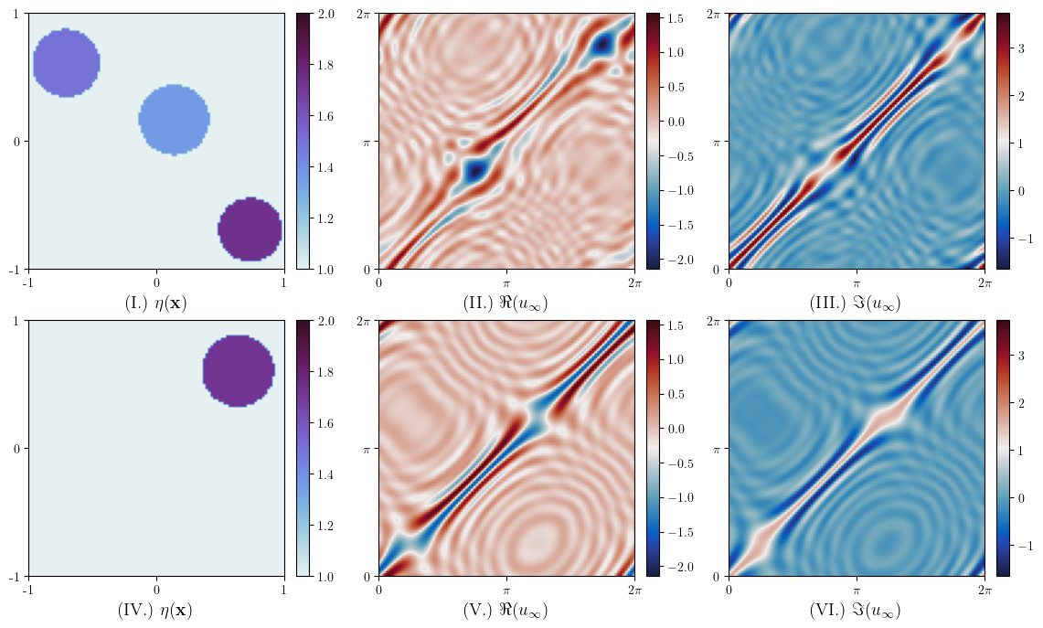
Figure 2: Two realizations of the random training data. Each row displays a density plot of $\eta$ for a sample scatterer (left panel) alongside the real and imaginary components of its computed far field pattern. The far field pattern is the data for the inverse scattering problem.

For training, we want to use simple scatterers. Here we create the scatterer field $\eta(\textbf{x})$ as the union of $N_{c}$ piecewise-constant circles overlaying a homogeneous background of air, where we uniformly sample $N_{c}\in\{1,2,3\}$. The $i$th circle is assigned a constant value $\eta_{i}$ sampled from the uniform distribution $\mathcal{U}(1.1,1.8)$, with the background air set to $\eta=1$ (we shall see that $\eta\approx 1.8$ is outside the weak scattering regime). The radius and position of each circle are sampled uniformly from $\mathcal{U}(0.1,0.3)$ and $\mathcal{U}(-0.7,0.7)$, respectively. In selecting the training data, for simplicity of mesh generation, we enforce that the circles cannot overlap and must be fully contained in the search domain $[-1,1]^{2}$. We generate 20,000 samples for training and validation (under an 80-20% split) with an additional 4,000 samples for testing purposes. Visualizations of typical training samples can be seen in Figure 2.

The validity of the Born approximation is contingent upon weak scattering of the incident field. Moreover, the convergence of the Neumann series (and hence the accuracy of the Born approximation) requires $\eta$ to be sufficiently close to unity. In the case of the synthetic dataset, the Born approximation fails when $\eta_{i}\gg 1$ for any circle, thus preventing an accurate inversion of (14). In particular, a direct inversion results in severe underestimates of the true contrast regardless of the chosen regularization parameter $\gamma$.

When weak scattering breaks down, the Born approximation also gives rise to artifacts when there is multiple scattering. Examples of poor reconstructions using the Born approximation are shown in Section 5. We seek to remediate these failures in the strong scattering case through corrective approaches using neural networks.

4 Network architecture and training

Throughout the rest of the paper we shall used two norms defined on vectors with $n$ components so that if $\vec{v}\in\mathbb{C}^{n}$ then the $\ell^{p}$ norm of $\vec{v}$ is

$$\|\vec{v}\|_{p}=\left(\sum_{j=1}^{n}|v_{j}|^{p}\right)^{1/p},\;p=1,2.$$

For arrays (in particular the array of pixel intensities for the image), we first reshape the array into a vector and then compute the corresponding vector norm as above. By abuse of notation we shall use $\|\cdot\|_{p}$ to indicate the norm of a vector or a matrix ($p=2$ is in fact the Frobenius norm of a matrix).

4.1 Correction strategies

We propose two methods for correcting the Born approximation: a pre-correction and a post-correction. Let $\vec{\mu}_{\rm exact}$ denote the exact nodal values for the (vectorized) contrast. There is an error $\vec{\tau}_{\mu}$ associated with both the convergence of the Neumann series and its truncation (the Born approximation). We may write

$$\mathcal{B}\vec{\mu}_{\rm exact}=\vec{u}_{\infty}+\vec{\tau}_{\mu}\mathrel{\mathop{:}}=\vec{u}_{\infty}^{\tau_{\mu}}.$$ (17)

where $\mathcal{B}$ is the stacked Born operator defined in (15), and $\vec{u}_{\infty}$ is the exact far field pattern. The factor $\vec{\tau}_{\mu}$ can be thought of as the discrepancy in the Born-obtained far field compared to the true (simulated) far field. A CNN is trained to predict $\vec{\tau}_{\mu}$, and this approach pre-corrects the far field data into a form suitable for the Born approximation to predict an accurate contrast. In particular

$$\mathcal{B}^{-1}_{\gamma}(\vec{u}_{\infty}^{\tau_{\mu}})=\mathcal{B}_{\gamma}^{-1}(\mathcal{B}\vec{\mu}_{\rm exact})\approx\vec{\mu}_{\rm exact}$$

provided that $\gamma$ is chosen correctly and $\vec{u}_{\infty}^{\tau_{\mu}}$ is learned appropriately. This is motivated by the approach in [15], where a neural network is employed to compensate for modeling errors introduced by approximate forward models.

The second strategy to correct the Born approximation is to obtain an accurate representation of $\varepsilon_{\mu}$, the discrepancy between the naive Born reconstruction and the true contrast. The factor $\varepsilon_{\mu}$ encompasses the far field behavior excluded by the Born approximation as well as the numerical error from the inversion scheme. We write

$$\varepsilon_{\mu}=\vec{\mu}_{\rm exact}-\mathcal{B}_{\gamma}^{-1}\vec{u}_{\infty},$$ (18)

where, as in (16), ${\mathcal{B}}_{\gamma}^{-1}$ denotes the regularized inverse of the Born operator. Once $\varepsilon_{\mu}$ is learned, an improved contrast estimate can be obtained through the simple formula

$$\vec{\mu}_{\rm exact}\approx\mathcal{B}^{-1}_{\gamma}\vec{u}_{\infty}+\mathcal{\varepsilon}_{\mu}.$$

This is the approach used in, for example, [23, 16] in a different context for correcting satellite data-based retrieval algorithms.

4.2 Training

For the two correction strategies, we can associate the following CNN-Born (CNNB) and Born-CNN (BCNN) models, respectively. The former performs the Born approximation on the corrected input far field while the latter performs the Born approximation on the labels of the training set. For a training set of size $N_{\rm train}$ we have the corresponding training regimes:

• CNNB: We consider data pairs $\{(\vec{u}_{\infty}^{(i)},\vec{u}^{\tau_{m}(i)}_{\infty})\}_{i=1}^{N_{\rm train}}$ and seek to minimize the loss function

  $$\mathcal{L}_{\rm CNNB}(\beta)=\frac{1}{N_{\rm train}}\sum_{i=1}^{N_{\rm train}}\|\vec{u}^{\tau_{\mu}(i)}_{\infty}-\operatorname{CNNB}(\vec{u}_{\infty}^{(i)};\beta)\|_{2}^{2},$$ (19)

  where $\rm CNNB(\>\cdot\>;\beta)$ is a CNN with weights and biases collected in the vector $\beta$.

• BCNN: We consider data pairs $\{(\vec{u}_{\infty}^{(i)},\varepsilon_{\mu}^{(i))}\}_{i=1}^{N_{\rm train}}$ and seek to minimize the loss function

  $$\mathcal{L}_{\rm BCNN}(\beta^{\prime})=\frac{1}{N_{\rm train}}\sum_{i=1}^{N_{\rm train}}\|\varepsilon_{\mu}^{(i)}-\operatorname{BCNN}(\vec{u}_{\infty}^{(i)};\beta^{\prime})\|_{2}^{2},$$ (20)

  where $\rm BCNN(\>\cdot\>;\beta^{\prime})$ is another CNN weights and biases collected in the vector $\beta^{\prime}$.

To provide a baseline for comparison, we train a simple black-box CNN to directly map the far field data to the solution of the inverse scattering problem motivated by [10]. In other words, we consider data-pairs $\{(\vec{u}_{\infty}^{(i)},\vec{\mu}^{(i)})\}_{i=1}^{N_{\rm train}}$ and minimize the loss function

$$\mathcal{L}_{\rm CNN}(\beta^{\prime\prime})=\frac{1}{N_{\rm train}}\sum_{i=1}^{N_{\rm train}}\|\vec{\mu}^{(i)}-{\rm CNN}(u_{\infty}^{(i)};\beta^{\prime\prime})\|_{2}^{2},$$ (21)

where $\rm CNN(\>\cdot\>,\beta^{\prime\prime})$ is a third CNN with weights and biases $\beta^{\prime\prime}$.

To aid comparison we use the same general CNN structure in all three cases, but optimize the network hyper-parameters to each case. Furthermore, we compute the basic regularized Born inverse (16) with regularization parameter $\gamma=1$ and $\gamma=0.1$ for a direct comparison of CNN results to the Born approximation.

Figure 3: The neural network architecture for the three models compared in this paper. (a) The CNN model directly maps the far field to the squared refractive index. (b) The regularized Born inverse is computed to obtain a rough estimate of the squared refractive index $\eta(\textbf{x})$, which is then corrected by the BCNN predicted $\varepsilon$. (c) The CNNB model pre-corrects the far field and then applies a regularized Born inverse to obtain the squared refractive index. Note that the necessary reshaping of the far field are omitted in this diagram, as well as the map $\mu\mapsto\mu+1=\eta$.

In all three approaches, the model takes as input a representation of the far field matrix, specifically, where the real and imaginary parts are separated and stored in two distinct channels, which enables the model to process both components simultaneously. The model output is then reshaped into a two-dimensional map corresponding to the discrepancy term. This end-to-end mapping from far field data to an image-like discrepancy allows the model to leverage spatial correlations in the data that are challenging to capture through purely analytic approaches. The structure of the three methods is visualized in Figure 3.

Table 1: Hyper-parameters selected by tuning the CNN, BCNN, and CNNB models.

	CNN	BCNN	CNNB
Conv2D Layers	4	4	4
Conv2D Channels	[296, 211, 152, 61]	[335, 33, 195, 65]	[125, 358, 426, 221]
FC Layers	3	1	1
FC Units	[537, 465, 419]	[971]	[576]
Activation	GELU	GELU	GELU

The architecture of each CNN was determined through a randomized search process, where 150 network configurations were generated, and the best-performing model was selected based on the lowest validation mean squared error (MSE). The randomization process involved varying hyper-parameters, including the number of convolution layers (ranging from 1 to 4) and the number of fully connected (FC) layers (ranging from 1 to 3). The number of channels per each convolution layer was randomly chosen between 16 and 512, while the number of units per FC layer was selected between 64 and 1024. Max pooling, with a fixed kernel size of 2, was applied after each convolutional layer.

For activation functions, we randomly selected from a set including Rectified Linear Unit (ReLU), LeakyReLU with a negative slope of 0.1, Gaussian Error Linear Unit (GELU), Sin, and Sigmoid. The last layer always used a linear activation function. All models were trained using the AdamW optimizer with an initial learning rate of 0.0005, adjusted via a learning rate scheduler that applied a 5% decay every 100 epochs. The models were trained with an early stopping patience of 50 epochs. Table 1 provides a summary of the tuned hyper-parameters.

5 Numerical experiments

5.1 In-distribution performance

Following the discussion in Section 3.1, we generated 4,000 in-distribution scatterers to evaluate model performance. Table 2 summarizes the average $\ell^{2}$ and $\ell^{1}$ errors of the test scatterer reconstructions, and Figure 4 shows the actual profile of one example of a test scatterer together with the reconstructions.

To make clear that the CNN based models outperform the inverse Born approximation by itself, Figure 5 visualizes the error distribution for the test samples. The results show that the three models–CNN, CNNB, and BCNN–significantly outperform the Born approximation in terms of accuracy, reducing the relative $\ell^{2}$ error by almost 50%.

The distribution of relative errors reveals that the CNN based models consistently produce low-error reconstructions, with a tightly clustered distribution around the mean, compared to the direct Born approximation. This suggests that the learning-based models generalize well within the in-distribution setting. In contrast, the Born approximation exhibits a broader and more skewed error distribution, highlighting its poor accuracy in reconstructing scatterers outside of the weak-scattering approximation.

Table 2: Average relative $\ell^{2}$ and $\ell^{1}$ error in the reconstruction of the contrast $\mu$ expressed as a percentage on the test dataset of $4,000$ scatterers. The rows labeled Born show the results of using the regularized inverse Born approximation. The CNNB model performs optimally in both $\ell^{2}$ and $\ell^{1}$.

	$\ell^{2}$ error (%)	$\ell^{1}$ error (%)
Born ($\gamma=1$)	67.0378	111.8617
Born ($\gamma=0.1)$	74.5836	152.5471
CNN	35.0081	76.5449
CNNB	34.2960	69.4069
BCNN	36.1794	91.2601

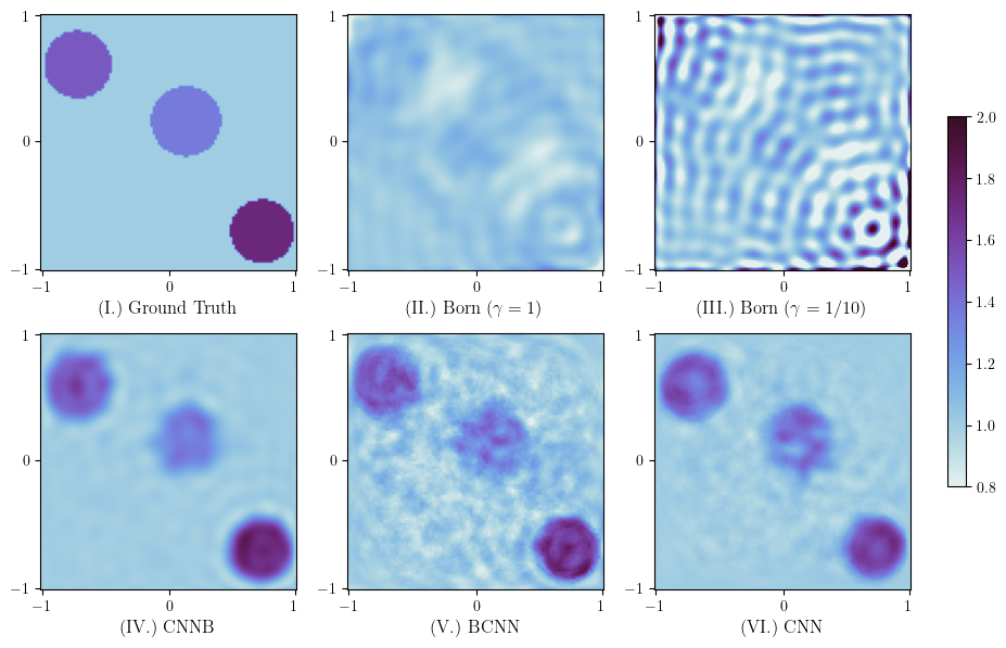
Figure 4: An example of the reconstructions of three circular scatterers determined by each model. Here we show density plots of the exact and reconstructed values of $\eta$. The ground truth is shown in the upper left panel. All CNN based methods are much more accurate than the inverse Born approximation since, in this example, the scattering is strong. CNNB (bottom left) shows the least speckle in the background.

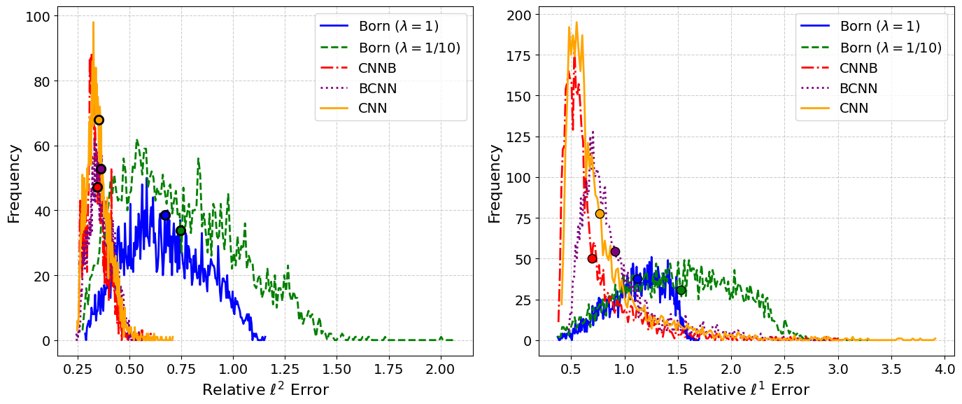
Figure 5: The distribution of relative $\ell^{2}$ (left) and $\ell^{1}$ (right) norm errors for the test dataset. The average of each distribution is denoted by the corresponding colored circle. The CNN based methods all improve over the simple Born approximation.

5.2 Noise robustness

Noise, arising from practical measurement apparatus errors or environmental factors, often corrupts scattering data, posing significant challenges to accurately reconstructing scatterers. We trained the CNNs using noise free data (apart from numerical error), so it is important to determine how the various CNN models cope with out-of-distribution data corresponding to far field patterns corrupted by noise. In this context, following [10], we consider a far field matrix affected by noise, with entries given by

$$(U^{\delta}_{\infty})_{i,j}\mathrel{\mathop{:}}=(1+\delta\mathcal{E}_{i,j})u_{\infty}(\hat{\textbf{x}}_{i},\textbf{d}_{j}),$$ (22)

where $\delta$ controls the strength of the noise and $\mathcal{E}_{i,j}$ is the (complex-valued) noise for incoming wave direction $\varphi_{i}$ and measurement direction $\theta_{j}$. To model the noise, we assume that $\mathcal{E}_{i,j}$ is sampled from a univariate complex standard normal distribution ${\cal CN}(0,1)$ [1, Def 2.1].

We analyze the zero-shot performance of the CNN, CNNB, and BCNN models under varying noise levels: $\delta=0$, $10\%$, $50\%$, $100\%$. We also compare their reconstructions to the Born model ($\gamma=1$), which is particularly robust to noise due to the regularized inversion, yet under-approximates the scatterer. At low noise levels ($\delta=0\%,\>10\%)$, all three CNN models demonstrate comparable and accurate reconstructions. However, as the noise level increases to 50%, significant differences emerge. The CNN and BCNN models suffer considerable performance degradation, with reconstructions marred by noticeable artifacts. At the extreme noise level of 100%, both models produce highly distorted results.

In contrast, the CNNB model exhibits remarkable robustness to noise, consistently producing accurate reconstructions with minimal artifacts even under high noise conditions. The regularized inversion incorporated into the CNNB algorithm effectively controls noise amplification and enables the optimized selection of regularization parameters. This capability demonstrates the model’s ability to reconstruct scatterers accurately in noisy environments. Figure 6 illustrates the comparative performance of the three models at different noise levels.

Figure 6: The inverse Born (first row), CNNB (second row), BCNN (third row), and CNN (fourth row) models for a small, strong circular test scatterer at noise level $\delta=0\%,\>10\%,\>50\%,\>100\%$. The Born approximation locates the scatterer correctly by greatly underestimates the contrast as is usual when applied to data from strong scatterers. Both BCNN and CNN suffer from poor artifacts at large noise levels.

5.3 Absorption

Our CNNs are trained on data from dissipation free media ($\Im(\eta)=0$). In many practical applications, the media exhibits varying degrees of dissipation or loss [12], characterized by $\Im(\eta)>0$. Since we did not train using far field data from dissipative scatterers, it is important to determine if we can predict the real part of $\eta$ even when the scattering media are slightly dissipative. The objective of this experiment is to evaluate the CNN models’ ability to accurately reconstruct $\Re(\eta(\textbf{x}))$ despite the presence of absorption in the true scatterer.

To investigate such scenarios, we consider the case in which $\eta$ inside the circle is perturbed by an unknown, small absorption term. Specifically, we use the following complex-valued $\eta$ to generate far field test data:

$$\eta^{\alpha}\mathrel{\mathop{:}}=\eta_{0}+\mathrm{i}\mkern 1.0mu\alpha$$ (23)

where $\alpha>0$ controls the strength of the perturbation and $\eta_{0}$ is the real part of the refractive index of the scattering medium. For this experiment, we fix $\eta_{0}=1.8$ in the scatterer. Since we assume that the background medium is air that is not absorbing, we do not add any absorption to the background, which remains at $\eta=1$. We specifically consider the cases where $\alpha=0,\>1/10,\>1,\>10$.

The results are shown in Figure 7. We observe that the CNNB architecture can effectively handle the exponential decay in the total field caused by absorption in the scatterer, making it a promising candidate for practical applications where absorption effects, though small, are present. In contrast, the BCNN and CNN networks are less stable to absorption and fail to preserve the shape of the scatterer for $\alpha=10$.

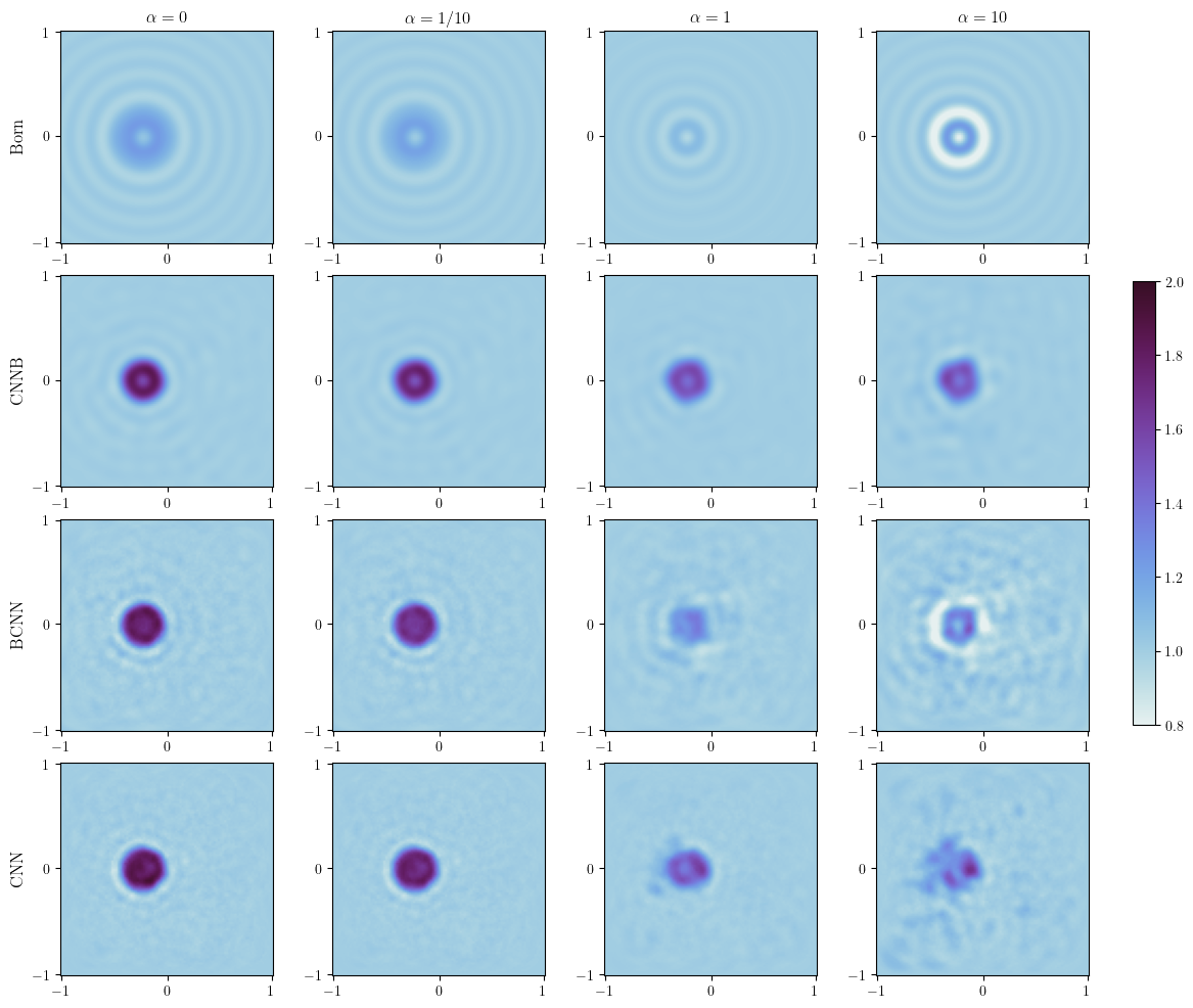
Figure 7: Results for a) the inverse Born approximation with $\gamma=1$ (first row), CNNB (second row), BCNN (third row), and CNN (fourth row) models for a small, strong circular scatterer having absorption parameter $\alpha=0,\>1/10,\>1,\>10$.

5.4 Increased scatterer complexity

We next evaluate the generalization capabilities of the CNN models when applied to more complex out-of-distribution scatterers. The scatterers are as follows:

1. A U-shaped scatterer chosen to resonate with the incident field (see top left panel in Figure 8). As we shall see, for this shape, the opening of the U is difficult to image using the inverse Born method.

2. A high-contrast annulus or ring inside a circle with an elliptic inclusion as shown in Figure 9. The goal with this example is to test if the CNN based schemes can detect the inner wall, even though they were trained on scattering by simple disks.

3. In potential biomedical applications, it is desirable to determine the refractive index of structures within other structures. In this example, we construct a scatterer akin to the Shepp-Logan phantom. High-contrast scatterers are placed within a high-contrast ring as shown in the top left hand panel of Figure  10. Restrictions on our mesh generator for the forward problem prevented us using the Shepp-Logan phantom itself. We also note that the values of $\eta$ used here are not the same as for the real Shepp-Logan phantom.

4. The CNN based methods are trained on smooth scatterers. Our last test uses a scatterer made of rectangles and an inner low contrast region (see top left panel in Figure 11).

The results of running the various reconstruction algorithms are summarized in Table 3 and in Figures 8–11 and are discussed next:

Table 3: Relative $\ell^{2}$ error in the reconstruction of $\mu$ as percentages for the inverse Born approximation and the three CNN models for the complex scatterers in Section 5.4. The best reconstruction for each problem is in boldface.

	Relative $\ell^{2}$ Error (%)
Method	U	Ring	Shepp	Rectangles
Born ($\gamma=0.1$)	92.72	106.26	104.44	87.68
Born ($\gamma=1$)	88.95	87.49	92.76	81.60
CNN	67.63	44.41	63.42	43.66
CNNB	60.53	41.23	60.03	39.28
BCNN	66.28	39.76	60.57	43.03

1. The results of reconstructing the high-contrast U-shaped resonant structure are shown in Figure  8 and Table 3. The inverse Born scheme exhibits artifacts and does not clearly show the U. While all three CNN models greatly improve on the Born approximation, the CNNB model preserves the shape of the U with minimal background artifacts. Meanwhile, the BCNN model constructs the scatterer with distortion in the surrounding media and the CNN model is blurred. The relative error in $\ell^{1}$ or $\ell^{2}$ conform that CNNB is best in this case.

2. Our second example, the high contrast ring scatterer, tests if it is possible to observe the inner structure of an object. As shown in Figure 9, the direct use of the inverse Born scheme does not reveal the inner ellipse. All three CNN models improve of the inverse Born, and perform relatively similarly in obtaining the shape. In this case, the BCNN model best approximates the true value of $\eta$ in the annulus as shown in Table 3.

3. Concerning the modified Shepp-Logan phantom, we see from Figure 10 and Table 3 that with appropriate regularization, the inverse Born scheme correctly images (though under-approximates) $\eta$ in the outer boundary of the scatterer, but fails to image structures inside. All CNN based methods improve over the inverse Born approximation, though the BCNN model well-approximates both the outer ring and the separation of the three internal scatterers, CNNB gives the best quantitative reconstruction.

4. We finally consider the shape constructed from several rectangles, possessing both sharp corners and an interior of air as shown in Figure 11 and Table 3. We see that the inner inclusion is invisible to the Born approximation, and the high contrast block is not well approximated. All three CNN models perform comparatively similarly, but the CNNB and BCNN models better approximate the shape of the internal region in comparison to the CNN and Born models. Quantitatively CNNB performs best. The presence of corners does not badly impact the CNN based models.

Overall we have demonstrated good generalization to a variety of scatterers not obviously connected to the training data. These results hint that training on simple shapes like circles is a successful strategy.

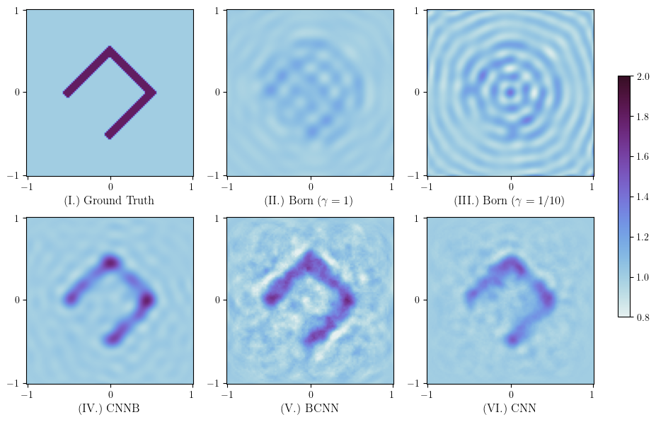
Figure 8: The reconstruction of a high-contrast, U-shaped resonance structure by the inverse Born approximation and the there CNN based schemes. All three CNN based schemes result in much clearer reconstructions with CNNB having less background noise than BCNN or CNN.

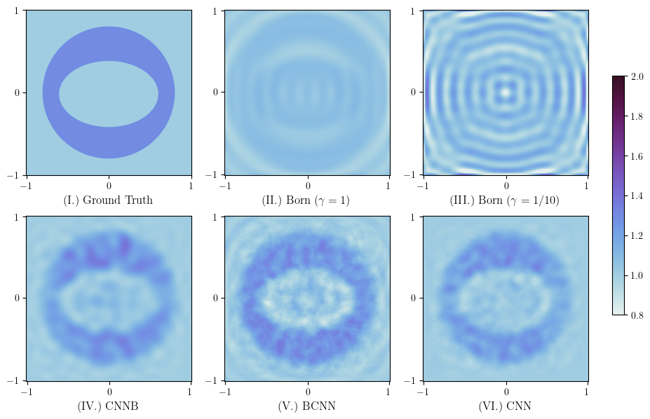
Figure 9: The reconstruction of a high-contrast annular scatterer. All three CNN based schemes are markedly better than inverse Born alone. With the CNN approach, the interior of the annulus can be reconstructed.

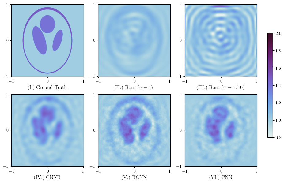
Figure 10: The reconstruction of a simplified Shepp-Logan-like phantom. Here the scattering ellipses are surrounded by a thin high contrast annulus of varying thickness. The Born approximation can detect this ring, but fails to reconstruct inside. All three CNN based schemes detect the three internal scatterers.

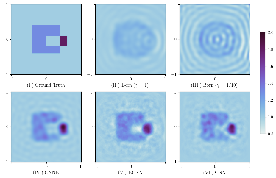
Figure 11: The reconstruction of a structure with sharp corners. The inner void is not seen in the Born reconstructions but is detected by the CNN schemes with CNNB and BCNN producing better reconstructions than CNN alone.

6 Conclusion

Our examples demonstrate that combining CNNs with the Born approximation can extend the applicability of the method beyond the weak scattering limit. All three CNN models can reveal the inner structure of high contrast objects better than the Born approximation. Moreover, a CNN combined with the inverse Born model always improves scatterer reconstruction in comparison to a pure CNN model. Because of it’s stability to noise and optimality for almost every test, we prefer the CNNB approach.

It is notable that we elected to train using simple shapes (disks), but the trained CNN models successfully generalize to more exotic cases.

Much more work needs to be done to extend this demonstration to a realistic biomedical problem like ultrasound tomography. For example, the current implementation of the regularized inverse Born approximate uses simple dense linear algebra to evaluate the necessary inverse. Fast methods should be used, such as the specialized neural network of [26] or the low-rank method of [25]. In addition, for specific applications, other simple training data could be considered (for example, if the goal is to image a network of blood vessels).

A particularly interesting direction for further work is to apply the method to more exotic measurement scenarios. For example, the case where both transmitters and receivers are on one side of the object, or when there is missing data from certain angular sectors. Moreover, additional work could include extending the applicability of the model to cases in which the wave number $k$ varies (i.e. multi-frequency data) or when the scattering medium is defined by a function that is not piecewise-constant.

References

- [1] H. H. Andersen, M. Højbjerre, D. Sørensen, and P. S. Eriksen, The Multivariate Complex Normal Distribution, Springer New York, New York, NY, 1995, pp. 15–37, https://doi.org/10.1007/978-1-4612-4240-6_2.
- [2] M. Born and E. Wolf, Principles of Optics, Pergamon Press, Cambridge, 1 ed., 1959.
- [3] F. Cakoni, D. Colton, and H. Haddar, Inverse Scattering Theory and Transmission Eigenvalues, SIAM, Philadelphia, USA, 2nd ed., 2022.
- [4] F. Chen, Z. Liu, G. Lin, J. Chen, and Z. Shi, NSNO: Neumann Series Neural Operator for solving Helmholtz equations in inhomogeneous medium, Journal of Systems Science and Complexity, 37 (2024), pp. 413–440, https://doi.org/10.1007/s11424-024-3294-x.
- [5] W. C. Chew and W. H. Weedon, A 3D perfectly matched medium from modified Maxwell’s equations with stretched coordinates, Microwave and Optical Technology Letters, 7 (1994), pp. 599–604, https://doi.org/10.1002/mop.4650071304.
- [6] D. Colton and R. Kress, Inverse Acoustic and Electromagnetic Scattering Theory, Springer-Verlag, New York, 4th ed., 2019.
- [7] G. Cybenko, Approximation by superpositions of a sigmoidal function, Mathematics of Control, Signals and Systems, 2 (1989), p. 303–314, https://doi.org/10.1007/BF02551274.
- [8] A. Devaney, Mathematical Foundations of Imaging, Tomography and Wavefield Inversion, Cambridge University Press, 2012.
- [9] A. J. Devaney, Inversion formula for inverse scattering within the Born approximation, Optics Letters, 7 (1982), pp. 111–112, https://doi.org/10.1364/OL.7.000111.
- [10] Y. Fan and L. Ying, Solving inverse wave scattering with deep learning, Annals of Mathematical Sciences and Applications, 7 (2022), pp. 23–24, https://doi.org/10.4310/AMSA.2022.v7.n1.a2.
- [11] J. A. Hudson and J. R. Heritage, The use of the Born approximation in seismic scattering problems, Geophysical Journal International, 66 (1981), pp. 221–240, https://doi.org/10.1111/j.1365-246X.1981.tb05954.x.
- [12] D. Jackson, Classical Electrodynmaics, Wiley, 3rd ed., 1988.
- [13] J. P. Kaipio, T. Huttunen, T. Luostari, T. Lähivaara, and P. B. Monk, A Bayesian approach to improving the Born approximation for inverse scattering with high-contrast materials, Inverse Problems, 35 (2019), p. 084001, https://doi.org/10.1088/1361-6420/ab15f3.
- [14] A. Kirsch, An Introduction to the Mathematical Theory of Inverse Problems, Springer, 2011.
- [15] J. Koponen, T. Lähivaara, J. Kaipio, and M. Vauhkonen, Model reduction in acoustic inversion by artificial neural network, The Journal of the Acoustical Society of America, 150 (2021), pp. 3435–3444, https://doi.org/10.1121/10.0007049.
- [16] A. Lipponen, J. Reinvall, A. Väisänen, H. Taskinen, T. Lähivaara, L. Sogacheva, P. Kolmonen, K. Lehtinen, A. Arola, and V. Kolehmainen, Deep-learning-based post-process correction of the aerosol parameters in the high-resolution Sentinel-3 level-2 Synergy product, Atmospheric Measurement Techniques, 15 (2022), pp. 895–914, https://doi.org/10.5194/amt-15-895-2022.
- [17] Z. Liu, F. Chen, J. Chen, L. Qiu, and Z. Shi, Neumann series-based neural operator for solving inverse medium problem, 2024, https://arxiv.org/abs/2409.09480.
- [18] P. Monk and E. Süli, The adaptive computation of far-field patterns by a posteriori error estimation of linear functionals, SIAM Journal on Numerical Analysis, 36 (1998), pp. 251–274, https://doi.org/10.1137/S0036142997315172.
- [19] S. Moskow and J. Schotland, Born and inverse Born series for scattering problems with Kerr nonlinearities, Inverse Problems, 39 (2023), https://doi.org/10.1088/1361-6420/ad07a5. 125015 (20pp).
- [20] S. Moskow and J. C. Schotland, Inverse Born series, in The Radon Transform: The First 100 Years and Beyond, R. Ramlau and O. Scherzer, eds., De Gruyter, Berlin, Boston, 2019, ch. 12, pp. 273–296, https://doi.org/10.1515/9783110560855-012.
- [21] J. Schöberl, NETGEN - An advancing front 2D/3D-mesh generator based on abstract rules, Computing and Visualization in Science, 1 (1997), pp. 41–52, https://ngsolve.org. (Current version).
- [22] A. Stanziola, S. R. Arridge, B. T. Cox, and B. E. Treeby, A Helmholtz equation solver using unsupervised learning: Application to transcranial ultrasound, Journal of Computational Physics, 441 (2021), p. 110430, https://doi.org/10.1016/j.jcp.2021.110430.
- [23] H. Taskinen, A. Väisänen, L. Hatakka, T. Virtanen, T. Lähivaara, A. Arola, V. Kolehmainen, and A. Lipponen, High-resolution post-process corrected satellite AOD, Geophysical Research Letters, 49 (2022), https://doi.org/10.1029/2022GL099733. Article: e2022GL099733.
- [24] Z. Wang, T. Cui, and X. Xiang, A neural network with plane wave activation for Helmholtz equation, 2020, https://arxiv.org/abs/2012.13870.
- [25] Y. Zhou, L. Audibert, S. Meng, and B. Zhang, Exploring low-rank structure for an inverse scattering problem with far field data. arXiv: https://arxiv.org/abs/2412.19724, 2024.
- [26] Z. Zhou, On the simultaneous recovery of two coefficients in the Helmholtz equation for inverse scattering problems via neural networks, Advances in Computational Mathematics, 52 (2025), https://doi.org/10.1007/s10444-025-10225-z. Art. No. 12.