Transferring between sparse and dense matching via probabilistic reweighting

Abstract

Detector-based and detector-free matchers are only applicable within their respective sparsity ranges. To improve adaptability of existing matchers, this paper introduces a novel probabilistic reweighting method. Our method is applicable to Transformer-based matching networks and adapts them to different sparsity levels without altering network parameters. The reweighting approach adjusts attention weights and matching scores using detection probabilities of features. And we prove that the reweighted matching network is the asymptotic limit of detector-based matching network. Furthermore, we propose a sparse training and pruning pipeline for detector-free networks based on reweighting. Reweighted versions of SuperGlue, LightGlue, and LoFTR are implemented and evaluated across different levels of sparsity. Experiments show that the reweighting method improves pose accuracy of detector-based matchers on dense features. And the performance of reweighted sparse LoFTR is comparable to detector-based matchers, demonstrating good flexibility in balancing accuracy and computational complexity.

1 Introduction

Feature matching is a fundamental technology of many computer vision applications such as structure from motion (SFM) [29], simultaneous localization and mapping (SLAM) [3] and re-localization [21]. Recent advancements in learning-based feature matching have led to the emergence of two paradigms: detector-based matching [27, 18] and detector-free matching [32, 12]. For a pair of images to be matched, detector-based methods first utilize a detector [9, 35] to extract two sparse sets of feature points from the images, and then compute point-to-point correspondences within these sets. On the other hand, detector-free methods compute dense feature maps of the images and directly use all features for matching.

The two matching paradigms differ in the sparsity of features and exhibit complementarity. Sparse matching in detector-based methods is more lightweight but prone to failures under significant variations in factors such as texture, viewpoint, illumination, and motion blur. Dense matching in detector-free methods can leverage more information from the images, thereby being more resilient to these factors, albeit at a higher computational cost. In practical applications, where diverse images pose varying degrees of matching difficulty, combining the two paradigms and dynamically adjusting the sparsity of matching according to the difficulty helps to balance precision and efficiency. However, the existing matching networks are only applicable within their respective sparsity ranges. Detector-based network struggles to improve accuracy through direct matching of high-density features, as shown in Fig. 1. Conversely, detector-free network is designed with their feature sparsity limited to the dense range.

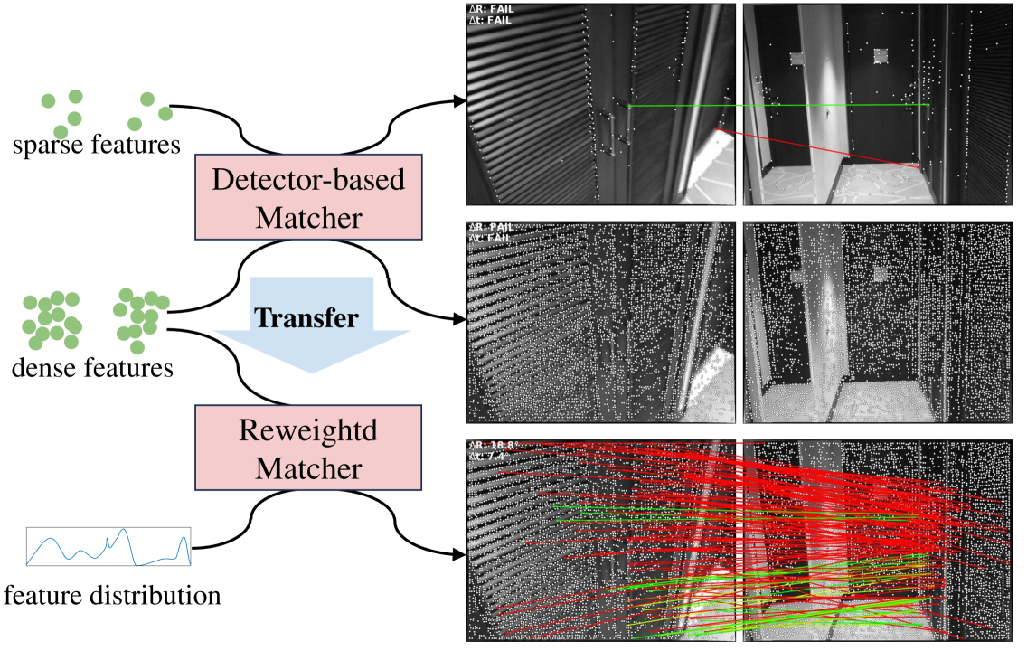
Figure 1: Transfer detector-based matcher to dense matching. The original detector-based matcher fails on the challenging image pair using either sparse or dense feature points. Given the feature distribution, the reweighted matcher alters attention scores at inference time and better match dense feature points. The results are from unmodified and reweighted SuperGlue using SuperPoint features.

It is noteworthy that the both matching paradigms employ attention mechanism [36], which is inherently able to process an arbitrary number of features. However, due to the different distributions of features in sparse and dense matching, simply altering the number of features matched by the network causes generalization issues. To adapt pretrained attention network to a matching scenario where feature sparsity exceeds the training sparsity range, we propose a reweighting method where the attention weights and matching scores are adjusted by feature detection probabilities. We derive the reweighted attention and matching function from a detector-based perspective, and prove that the reweighted matching network is the asymptotic limit of conventional matching network. Based on our reweighting method, existing detector-based networks are transferred to a dense matching paradigm while preserving the distribution of features sampled from the detector. We also propose a sparse training and pruning pipeline for detector-free networks, optimizing the feature distribution to allow them to perform efficient sparse matching.

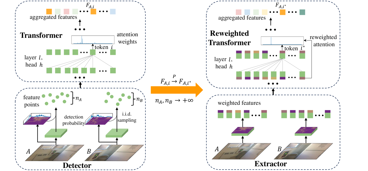
Figure 2: Probabilistic derivation of reweighted Transformer. The left side depicts the conventional detector-based feature matching, where the detector extracts features and computes detection probabilities for keypoints. A Transformer is utilized to aggregate the keypoints sampled by the detector. The right side illustrates the reweighted attention network that employs features with probability weights and adjusts attention weights based on the probabilities. The reweighted matching network is the asymptotic limit of conventional matching network: for i.i.d. keypoints, as the sample size approaches infinity, the features aggregated by the original network converge in probability to those aggregated by the reweighted network.

Our reweighted attention function is applicable to a wide range of Transformers and adapts them to varying sparsity levels without altering network parameters. We reweight the mainstream SuperGlue, LightGlue, and LoFTR and transfer them to matching tasks at different sparsity levels. Their performances in relative pose estimation and visual localization are evaluated. Results indicate that the reweighted detector-based matchers surpass their sparse performance through dense matching. The reweighted LoFTR achieves sparse matching performance comparable to that of detector-based matchers while maintaining dense performance. Furthermore, we illustrate that sparse training of LoFTR can generate edge detector and salient point detector, demonstrating high adaptability.

2 Related Work

Detector-based Matching.  Classical detector-based matching methods focus on designing keypoints [20, 2, 14, 25], with correspondences obtained through nearest neighbor search and outlier removal method [13]. These methods rely on domain-specific knowledge and are prone to failure when the actual data distribution does not conform to their underlying assumptions. Recent approaches train neural networks for keypoint detection and description [9, 10, 23, 35, 15, 1]. Among them, SuperPoint [9] interprets the output of keypoint detectors from a probabilistic perspective, while DISK [35] employs a probabilistic method to relax cycle-consistent matching, thereby simplifying the training.

The matching quality of nearest neighbor is constrained due to the limited utilization of keypoint information. Learning-based feature matching methods have been proposed to better match keypoints. SuperGlue [27] uses a Graph Neural Network (GNN), specifically a Transformer [36], to aggregate the features of keypoints to be matched. Subsequent works [4, 30, 18] have adopted the Transformer structure and sought to enhance its efficiency. Notably, LightGlue [18] enables adaptive computation and demonstrates gains in both efficiency and accuracy.

Detector-free Matching.  Unlike detector-based matching, detector-free matching employs dense descriptors or features of images for matching. SIFT Flow [19] achieves scene alignment using densified classical descriptors. Early learning-based methods utilize contrastive loss to learn dense descriptors [6, 28]. More recent approaches learn dense matching using dense 4D cost volumes [24, 16, 34]. LoFTR [32] and followups [37, 5, 40, 22, 38] leverage Transformers to aggregate image features. LoFTR performs dense matching on low-resolution feature map in coarse stage, and PATS [22] extends the dense matching to input resolution. DKM and RoMa using gaussian processes also achieve dense matching at the input resolution [11, 12].

3 Methodology

We focus on image matchers using Transformers and revisit the matching pipeline. Then we derive probabilistic reweighted attention and matching functions from a detector-based perspective and prove their asymptotic equivalence to the original functions. The probabilistic derivation of reweighted Transformer is illustrated in Fig. 2. Based on reweighting method, we transfer existing matchers between sparse and dense paradigms.

3.1 Preliminaries

Both sparse and dense image matching use image features, where a backbone is employed to compute feature map $\mathbf{D}$. In sparse matching, feature points are detected and sampled from the feature map before matching. On the other hand, dense matching directly computes correspondences using the entire feature map.

Given an image $I$, the probability that a pixel coordinate $x$ is detected as a feature point is denoted as $P(x|I,\theta_{F})$, where $\theta_{F}$ represents the parameters of the feature detector. The feature or descriptor at $x$ is denoted as $\mathbf{D}(x)$. A sequence of i.i.d. coordinates $\{x_{n}\}$ from $P(x|I,\theta_{F})$ yields a sequence of feature points $F_{I}=\{(x_{1},\mathbf{D}(x_{1})),(x_{2},\mathbf{D}(x_{2})),...,(x_{n},\mathbf{D}(x_{n}))\}$. We denote $F_{I}^{*}$ as an ordered set of all possible feature points form $\mathbf{D}$. Let the $i$-th point in $F_{I}$ be $F_{I,i}$. For each index $i$, there is a corresponding index $i^{*}$ in $F_{I}^{*}$ such that $F_{I,i}=F_{I,i^{*}}^{*}$.

For images $A$ and $B$, sparse matching establishes correspondences between a limited number of feature points $F_{A}$ and $F_{B}$, while dense matching involves matching $F_{A}^{*}$ and $F_{B}^{*}$ without probabilistic sampling. In both sparse and dense matching, the features are first aggregated utilizing Transformers, followed by the computation of assignment matrices through matching functions. Due to the different feature distributions, sparse and dense matching Transformers are typically isolated, with distinct sets of parameters. We denote $\mathrm{TF_{sparse}}$ and $\mathrm{TF_{dense}}$ as sparse and dense matching Transformers respectively. The aggregated feature points are expressed as

$$\begin{split}&(F_{A}^{\prime},F_{B}^{\prime})=\mathrm{TF_{sparse}}(F_{A},F_{B})\\ &(F_{A}^{*^{\prime}},F_{B}^{*^{\prime}})=\mathrm{TF_{dense}}(F_{A}^{*},F_{B}^{*}),\end{split}$$ (1)

where the order of feature points in each sequence is maintained. For each index $i$, $F_{A,i}^{\prime}$ is the update of $F_{A,i}$, whose descriptor is replaced by corresponding token of the network’s last layer. The same applies to $F_{B}$, $F_{A}^{*}$ and $F_{B}^{*}$.

3.2 Reweighted Attention

Matching Transformers aggregate features using an embedding layer and multiple attention layers. Given feature points $F_{A}$ and $F_{B}$ with cardinalities of $n_{A}$ and $n_{B}$, the embedding layer map feature points to tokens, $\mathbf{X}_{A}\in\mathbb{R}^{d\times n_{A}}$, $\mathbf{X}_{B}\in\mathbb{R}^{d\times n_{B}}$, where $d$ is the number of feature channels. For each attention layer, the input tokens are denoted as $\mathbf{X}_{Q}$, $\mathbf{X}_{K}$ and $\mathbf{X}_{V}$. The output token $\mathbf{X}_{Q}^{\prime}$ is computed as follows:

$$\begin{split}&\mathbf{X}^{\prime}=\mathbf{X}_{Q}+\sum_{h=1}^{H}\mathbf{W}_{VO}^{h}\mathbf{X}_{V}\mathrm{Sim}(\mathbf{W}_{K}^{h}\mathbf{X}_{K},\mathbf{W}_{Q}^{h}\mathbf{X}_{Q})\\ &\mathbf{X}_{Q}^{\prime}=\mathbf{X}^{\prime}+\mathbf{W}_{2}\mathrm{Act}(\mathbf{W}_{1}\mathbf{X}^{\prime}+\mathbf{b}_{1}\mathbf{1}^{\top})+\mathbf{b}_{2}\mathbf{1}^{\top}\end{split}$$ (2)

where $H$ is the number of attention heads, and $\mathbf{W}_{VO}^{h}$, $\mathbf{W}_{K}^{h}$, and $\mathbf{W}_{Q}^{h}$ are parameter matrices of the $h$-th attention head. In feed forward part, $\mathbf{W}_{1},\mathbf{W}_{2}$ and $\mathbf{b}_{1},\mathbf{b}_{2}$ are parameter matrices and vectors respectively, and all ones vector $\mathbf{1}$ broadcasts parameter vectors to match the shape of tokens. The attention matrix is obtained by calculating the query and key matrices with the function $\mathrm{Sim}$. The activation function $\mathrm{Act}$ can be any continuous element-wise function.

Definition 1.

Let $\delta$ be a similarity function that map $\mathbb{R}^{d}\times\mathbb{R}^{d}$ into $\mathbb{R}$. Given key and query matrices $\mathbf{K}\in\mathbb{R}^{d\times n_{K}},\mathbf{Q}\in\mathbb{R}^{d\times n_{Q}}$, denote their column vectors as $\mathbf{K}_{i}$ and $\mathbf{Q}_{j}$. Then the attention matrix $\mathrm{Sim}(\mathbf{K},\mathbf{Q})\in\mathbb{R}^{n_{K}\times n_{Q}}$ is defined such that

$$\mathrm{Sim}_{i,j}(\mathbf{K},\mathbf{Q})=\frac{{\delta({\mathbf{K}_{i}},{\mathbf{Q}_{j}})}}{{\sum\limits_{k=1}^{{n_{K}}}{\delta({\mathbf{K}_{k}},{\mathbf{Q}_{j}})}}},\\$$ (3)

where $\mathrm{Sim}_{i,j}$ is the element in its $i$-th row and $j$-th column, $1\leq i\leq{n_{K}},1\leq j\leq{n_{Q}}$.

In standard attention where Softmax is employed, the similarity function is

$$\delta_{softmax}({\mathbf{K}_{i}},{\mathbf{Q}_{j}})=\exp(\tau^{-1}{\mathbf{K}_{i}}^{\top}{\mathbf{Q}_{j}}),$$ (4)

where $\tau$ is temperature parameter. In linear attention, the similarity function is

$$\delta_{linear}({\mathbf{K}_{i}},{\mathbf{Q}_{j}})=\phi({\mathbf{K}_{i}})^{\top}\phi({\mathbf{Q}_{j}}),$$ (5)

where $\phi$ is a continuous element-wise function.

Definition 2.

Given key and query matrices $\mathbf{K}$ and $\mathbf{Q}$, $\mathbf{K}\in\mathbb{R}^{d\times n_{K}},\mathbf{Q}\in\mathbb{R}^{d\times n_{Q}}$. The probability weights associated with each column of the key matrix are denoted as $p_{I}(i)$, $p_{I}(i)=P(x_{i}|I,\theta_{F}),1\leq i\leq n_{K}$, where $I$ is the image corresponding to the key matrix. Then the reweighted attention matrix $\mathrm{Sim}^{p}(\mathbf{K},\mathbf{Q})\in\mathbb{R}^{n_{K}\times n_{Q}}$ is defined such that

$$\mathrm{Sim}_{i,j}^{p_{I}}(\mathbf{K},\mathbf{Q})=\frac{p_{I}(i){\delta({\mathbf{K}_{i}},{\mathbf{Q}_{j}})}}{{\sum\limits_{k=1}^{{n_{K}}}p_{I}(k){\delta({\mathbf{K}_{k}},{\mathbf{Q}_{j}})}}}.$$ (6)

For image $A$, $B$ and probability weights $p_{A}$, $p_{B}$, the reweighted Transformer $\mathrm{TF}^{p_{A},p_{B}}$ of network $\mathrm{TF}$ is defined as follows: while keeping the parameters unchanged, the attention function of each attention layer is replaced with the reweighted version. In each reweighted attention, the weights $p_{A}$ or $p_{B}$ are used based on whether the token $\mathbf{X}_{K}$ corresponds to the image $A$ or $B$, respectively.

We introduce the following theorem that reveals the asymptotic equivalence of the reweighted network and the original network:

Theorem 1.

Let $F_{A}$ and $F_{B}$ be two sequences of i.i.d. feature points, which are sampled from $F_{A}^{*}$ and $F_{B}^{*}$ according to detection probabilities $p_{A}$ and $p_{B}$, respectively. Let $\mathrm{TF}$ and $\mathrm{TF}^{p_{A},p_{B}}$ be any attention network and its reweighted version, as described above. And the feature points are aggregated as described in Eq. 1, where $\mathrm{TF_{sparse}}=\mathrm{TF}$ and $\mathrm{TF_{dense}}=\mathrm{TF}^{p_{A},p_{B}}$. For any index pair $i$ and $j$, denote $i$-th and $j$-th output feature points from network $\mathrm{TF}$ as $\mathrm{TF}_{i,j}$, i.e., $\mathrm{TF}_{i,j}(F_{A},F_{B})=(F^{\prime}_{A,i},F^{\prime}_{B,j})$. As the sizes of $F_{A}$ and $F_{B}$ tend to infinity, we have

$$\mathrm{TF}_{i,j}(F_{A},F_{B})\stackrel{{\scriptstyle P}}{{\longrightarrow}}\mathrm{TF}_{i^{*},j^{*}}^{p_{A},p_{B}}(F_{A}^{*},F_{B}^{*}).$$ (7)

The theorem states that as the number of sampled feature points approaches infinity, the features obtained by directly aggregating these feature points with an attention network converge in probability to the features obtained by processing the feature map with the reweighted network. The proof of this theorem can be found in Appendix.

3.3 Reweighted Matching Function

Matching function computes an assignment matrix $\mathbf{P}$ of all possible matches. Frequently employed matching layers leverage features from multi-layer attention to compute $\mathbf{P}$, whereas in reweighted matching layers, the functions incorporate the probabilities of these features as well. We introduce two types of reweighted matching functions with optimal transport and dual-softmax. Then we demonstrate their asymptotic equivalence to original functions through a probabilistic convergence theorem.

For aggregated feature points $F_{A}^{{}^{\prime}}$ and $F_{B}^{{}^{\prime}}$, denote the $i$-th and $j$-th feature vectors as $\mathbf{f}_{A,i}$ and $\mathbf{f}_{B,j}$, then a score matrix $\mathbf{S}$ is defined as pairwise inner product of the feature vectors:

$$\mathbf{S}_{i,j}=\mathbf{f}_{A,i}^{\top}\mathbf{f}_{B,j}.$$ (8)

For matching function with optimal transport, the score matrix $\mathbf{S}$ is augmented to $\overline{\mathbf{S}}$ by appending a new row and column filled with a dustbin score, as in [27]. The probabilistic weight vectors of $A$ and $B$ are denoted as $\mathbf{a}$ and $\mathbf{b}$, $\mathbf{a}\in\mathbb{R}^{n_{A}+1},\mathbf{b}\in\mathbb{R}^{n_{B}+1}$ where the last component of each vector represents the dustbin:

$$\begin{split}&\mathbf{a}_{i}=p_{A}(i),\mathbf{a}_{n_{A}+1}=1,1\leq i\leq n_{A}\\ &\mathbf{b}_{j}=p_{B}(j),\mathbf{b}_{n_{B}+1}=1,1\leq j\leq n_{B}.\end{split}$$ (9)

The reweighted optimal transport layer finds an augmented assignment $\overline{\mathbf{P}}$ to maximize the total score $\sum_{i,j}\overline{\mathbf{S}}_{i,j}\overline{\mathbf{P}}_{i,j}$ with the following constrains:

$$\overline{\mathbf{P}}\mathbf{1}_{n_{B}+1}=\mathbf{a}\quad and\quad\overline{\mathbf{P}}^{\top}\mathbf{1}_{n_{A}+1}=\mathbf{b}.$$ (10)

In practice, the optimal transport layer utilizes the Sinkhorn algorithm [31, 7] to compute soft assignments. We define $\mathrm{OT}^{p_{A},p_{B}}(F_{A}^{\prime},F_{B}^{\prime})$ as the assignment computed by the layer, with $F_{A}^{\prime}$ and $F_{B}^{\prime}$ being the features and $p_{A}$ and $p_{B}$ being the probabilities associated with those features, respectively. When $p_{A}$ and $p_{B}$ are uniform distributions, the output assignment is denoted as $\mathrm{OT}(F_{A}^{\prime},F_{B}^{\prime})$, which differs from the assignment of matching layer in [27] by a constant factor.

For matching function with dual-softmax, denote $z_{i,j}$ as $\exp(\mathbf{S}_{i,j})$. The assignment $\mathrm{DS}^{p_{A},p_{B}}(F_{A}^{\prime},F_{B}^{\prime})$ of reweighted dual-softmax is defined as:

$$\mathrm{DS}_{i,j}(\mathbf{S})=\frac{p_{A}(i)p_{B}(j)z_{i,j}^{2}}{{\sum\limits_{k=1}^{{n_{A}}}p_{A}(k){z_{i,k}}\sum\limits_{l=1}^{{n_{B}}}p_{B}(l){z_{l,j}}}}.$$ (11)

Theorem 2.

Let $F_{A}^{\prime}$ and $F_{B}^{\prime}$ be two sequence of i.i.d. feature points which are sampled from $F_{A}^{*^{\prime}}$ and $F_{B}^{*^{\prime}}$ according to detection probabilities $p_{A}$ and $p_{B}$, respectively. For any index pair $i^{*}$ and $j^{*}$ of $F_{A}^{*^{\prime}}$ and $F_{B}^{*^{\prime}}$, as the sizes of $F_{A}^{\prime}$ and $F_{B}^{\prime}$ tend to infinity, we have

$$\sum_{\begin{subarray}{c}k,l:\\ k^{*}=i^{*},l^{*}=j^{*}\end{subarray}}\mathrm{OT}_{k,l}(F_{A}^{\prime},F_{B}^{\prime})\stackrel{{\scriptstyle P}}{{\longrightarrow}}\mathrm{OT}_{i^{*},j^{*}}^{p_{A},p_{B}}(F_{A}^{*^{\prime}},F_{B}^{*^{\prime}}).$$ (12)

$$\sum_{\begin{subarray}{c}k,l:\\ k^{*}=i^{*},l^{*}=j^{*}\end{subarray}}\mathrm{DS}_{k,l}(F_{A}^{\prime},F_{B}^{\prime})\stackrel{{\scriptstyle P}}{{\longrightarrow}}\mathrm{DS}_{i^{*},j^{*}}^{p_{A},p_{B}}(F_{A}^{*^{\prime}},F_{B}^{*^{\prime}}).$$ (13)

Therefore, the detector-based matching network, after reweighting its attention and matching functions using detection probabilities, can be transferred to dense features while retaining the knowledge about probabilistic importance of the features.

3.4 Sparsity Transfer

After reweighting the matcher, we perform seamless network transfer to different sparsity levels.

To enable existing detector-free matcher to perform sparse matching, we propose a straightforward sparse training and pruning pipeline based on the reweighting method, as shown in Fig. 3.

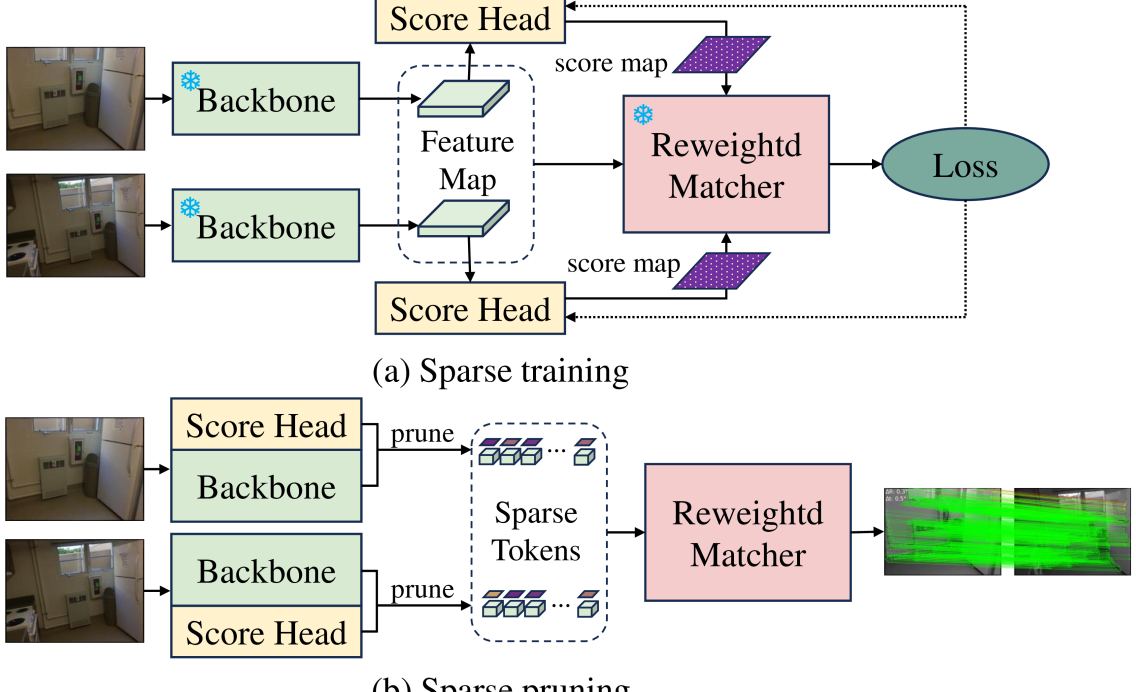
Figure 3: Sparse training and pruning of detector-free matcher. Using reweighted attention and matching function, we employ: (a) Sparse training with frozen backbone and matcher, (b) Sparse pruning for efficient inference.

During sparse training, we introduce a shallow score head between the backbone and the attention-based matching network. And we freeze the parameters of the network except for the score head to retain the dense matching capability. For each feature map, the score head computes a score map $\mathbf{S}$ assigning each feature a score between 0 and 1, representing the probability $P(x|I,\theta_{F})$ in Sec. 3.1. The matching network then performs reweighted attention and matching based on the feature map and the score map. And the matching loss $L_{m}$ is computed. Additionally, to sparsify the score map, we compute a sparsity loss $L_{s}=\left\lVert\mathbf{S}\right\rVert_{1}$. The total loss is $L_{m}+\lambda L_{s}$, where $\lambda$ is a hyperparameter controlling the degree of sparsity.

To enable dense matching using existing detector-based matchers, we augment the set $F_{I}^{*}$ of available feature points. And we treat the confidence scores computed by the detector as $P(x|I,\theta_{F})$ to weight the feature points. To utilize as many features as possible while staying within the limits of memory, we consider dense matching at the feature map resolution: we set the number of feature points in $F_{I}^{*}$ to be equal to the number of features in the feature map, with the spacing between feature points approximating the size of the image patches corresponding to each feature. We also employ non-maximum suppression to control the spacing between feature points and retain the feature point localization capability of the detector. When the feature map is excessively large, we use fewer features, which we term as semi-dense matching.

4 Experiments

We implement reweighted versions of mainstream matchers that utilize Transformers and evaluate their performances across different levels of sparsity. The comparisons of the sparse and dense matching performance are conducted on both indoor and outdoor datasets.

4.1 Relative Pose Estimation

We evaluate the relative pose estimation capability of feature matchers at different levels of sparsity. ScanNet [8] and MegaDepth [17] are utilized for indoor and outdoor assessment, respectively.

Settings.  ScanNet comprises image pairs with wide baselines and texture-less regions. We use 1500 test image pairs from ScanNet as in [27], with all images resized to $640\times 480$.

MegaDepth contains image pairs featuring drastic viewpoint changes and texture repetitions. We adhere to the testing procedure outlined in [18] and utilize 1500 test image pairs from St. Peters Square and Reichstag of MegaDepth for evaluation.

We evaluate SuperGlue, LightGlue, LoFTR, and their reweighted versions. To reweight the matchers, we use official models with their original parameters intact, modifying only the attention scores based on the probabilistic scores of features, as in Eq. 6. The reweighted SuperGlue and LightGlue utilize features and their probabilistic scores from SuperPoint or DISK. And we turn off the pruning mechanisms of LightGlue. The reweighted LoFTR utilizes the features provided by its backbone and computes sparse probabilistic scores using additionally trained score heads.

For evaluation of sparse matching performance, we compare the reweighted LoFTR against existing sparse matchers. The original SuperGlue and LightGlue are evaluated as baselines. On ScanNet, we extract 1024 features per image as in official implementation of  [27]. On MegaDepth, we extract 2048 features per image, as detailed in  [18].

For evaluation of dense matching performance, we compare the performance of reweighted SuperGlue and LightGlue with dense features. On ScanNet, we consider dense matching on feature maps at 1/8 of the input resolution and extract 4800 feature points with the highest probabilistic scores as dense features. On MegaDepth, we resize the longest side of the input images to 1600 pixels. At this resolution, we extract 12288 feature points with the highest probabilistic scores as semi-dense features. The remaining feature extraction and matching parameters are consistent with those used for sparse matching. Additionally, we evaluate the performance of the original LoFTR.

The pose error is computed as the maximum angular error in rotation and translation and reported as Area Under the Curve (AUC) at thresholds of 5°, 10°, and 20°. To obtain camera poses, we solve the essential matrix using RANSAC based on the matcher’s outputs.

Results of indoor pose estimation.  The results are shown in Tab. 1, where methods marked with (R) indicate those that are reweighted. In the sparse matching mode, the reweighted LoFTR achieves comparable performance to SuperPoint+LightGlue. In the dense matching mode, SuperPoint+SuperGlue is the most accurate among detector-based matchers. It is noteworthy that LoFTR not only achieves high dense matching accuracy, but also reaches comparable accuracy to the detector-based methods in sparse matching. This may be attributed to the feature selection ability learned by the network from indoor data with weak textures. Although detector-based matchers are weaker than LoFTR in dense matching, using the additional information provided by dense features can surpass the accuracy of sparse matching.

Sparsity	Method	Pose estimation AUC
		@5°	@10°	@20°
Sparse	SP+SuperGlue	14.72	32.58	50.85
	SP+LightGlue	13.71	29.11	45.64
	DISK+LightGlue	12.19	25.27	40.43
	LoFTR(R)	14.46	30.26	47.10
Dense	SP+SuperGlue(R)	15.67	34.97	55.17
	SP+LightGlue(R)	12.82	27.54	44.03
	DISK+LightGlue(R)	13.67	28.89	45.36
	LoFTR	22.06	40.80	57.62

Table 1: Evaluation for indoor pose estimation at different sparsity.

Results of outdoor pose estimation.  The outdoor results are presented in Tab. 2. Different from indoor scenes, the reweighted LoFTR is less accurate than detector-based matchers in the sparse matching mode. In the dense matching mode, DISK+LightGlue is the most accurate among detector-based matchers and approaches the accuracy of LoFTR. It can be observed that some detector-based dense matchers struggle to surpass their sparse variants when applied to outdoor data. This is because MegaDepth, characterized by its abundant textures, renders sparse features sufficient for accurate matching. The information gain provided by dense matching is insufficient to counteract the impact of feature confusion and generalization issues.

Sparsity	Method	Pose estimation AUC
		@5°	@10°	@20°
Sparse	SP+SuperGlue	48.97	66.80	79.99
	SP+LightGlue	51.50	68.17	80.60
	DISK+LightGlue	46.85	64.13	77.24
	LoFTR(R)	45.31	61.56	73.83
Semi-dense	SP+SuperGlue(R)	46.32	63.90	78.11
	SP+LightGlue(R)	48.30	65.62	79.31
	DISK+LightGlue(R)	51.01	67.66	80.05
	LoFTR	52.80	69.19	81.18

Table 2: Evaluation for outdoor pose estimation at different sparsity.

4.2 Visual Localization

We evaluate long-term visual localization under semi-dense features. The Aachen Day-Night [39] dataset and the InLoc [33] dataset are utilized for indoor and outdoor evaluations, respectively.

Settings.  We generate results for all methods using the HLoc[26] toolbox with default settings for triangulation, image retrieval, RANSAC, and Perspective-n-Point solver. The original matchers are evaluated as baselines and the feature extraction and matching settings provided by HLoc are adopted. The original SuperGlue and LightGlue perform sparse matching, while the original LoFTR performs semi-dense matching with a maximum number of feature points per image limited to 8192. To transfer the detector-based matchers to a sparsity level comparable to LoFTR, we increase the number of feature points per image to 8192 and reweight the matcher.

Results.  Outdoor evaluation results are shown in Tab. 3. For daytime data, the reweighted semi-dense matchers perform similarly to the original matchers. For nighttime data, the reweighted semi-dense matchers with SuperPoint outperform their sparse counterparts. LoFTR is less accurate than sparse matchers on daytime data but is more accurate on nighttime data. Intriguingly, after being transferred to semi-dense features, detector-based matchers demonstrate better generalization than LoFTR on nighttime data.

Results of indoor data are presented in Tab. 4. Similar to relative pose estimation, reweighted semi-dense matching achieves higher performance gains on indoor data compared to outdoor data. More stable performance gains are observed at lower distance thresholds, with reweighted SuperGlue surpassing LoFTR at (0.25m,10°).

Method	Day	Night
	(0.25m,2°) / (0.5m,5°) / (1.0m,10°)
SP+SuperGlue	90.4 / 96.5 / 99.3	76.4 / 91.1 / 100.0
SP+SuperGlue(R)	90.3 / 96.2 / 99.2	77.5 / 91.1 / 99.5
SP+LightGlue	90.3 / 96.1 / 99.3	77.0 / 91.6 / 100.0
SP+LightGlue(R)	90.4 / 96.5 / 99.2	77.5 / 92.1 / 100.0
DISK+LightGlue	88.1 / 95.5 / 99.3	76.4 / 90.1 / 99.5
DISK+LightGlue(R)	88.6 / 96.1 / 99.4	74.9 / 90.6 / 99.5
LoFTR	88.8 / 95.8 / 98.8	77.5 / 91.1 / 99.5

Table 3: Evaluation for visual localization on the Aachen Day-Night [39] benchmark v1.1. Methods marked with (R) indicate reweighted semi-dense matching.

Method	DUC1	DUC2
	(0.25m,10°) / (0.5m,10°) / (1.0m,10°)
SP+SuperGlue	46.0 / 65.7 / 79.3	47.3 / 71.0 / 77.1
SP+SuperGlue(R)	47.5 / 69.2 / 80.8	53.4 / 67.9 / 74.8
SP+LightGlue	42.9 / 64.1 / 76.3	42.0 / 66.4 / 72.5
SP+LightGlue(R)	43.9 / 67.7 / 80.3	48.9 / 69.5 / 77.1
DISK+LightGlue	42.4 / 59.6 / 73.7	36.6 / 56.5 / 68.7
DISK+LightGlue(R)	43.4 / 64.1 / 77.8	38.9 / 55.7 / 65.6
LoFTR	46.0 / 69.7 / 82.3	48.9 / 74.0 / 81.7

Table 4: Evaluation for visual localization on the InLoc [33] benchmark. Methods marked with (R) indicate reweighted semi-dense matching.

4.3 Comparison with Direct Dense Matching

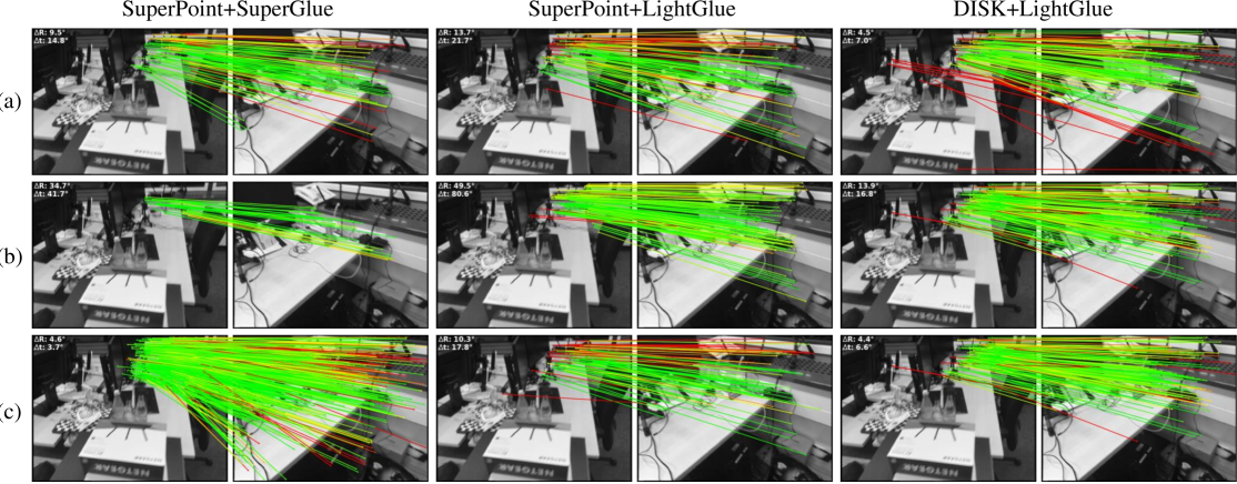
Figure 4: Comparison with direct matching. (a) Results of direct matching on sparse feature points. (b) Results of direct matching on dense feature points. (c) Results of reweighted matching on the same dense feature points. Matchers trained on sparse features encounter generalization issues when directly matching dense features, resulting in larger pose errors. Without additional training, the reweighted matchers generalize better to dense features, achieving lower pose errors.

In Sec. 4.1, a subset of reweighted detector-based matchers exhibit superior performance in dense matching modes compared to their sparse matching modes. This suggests that the information gain from additional features outweighs the detrimental effects stemming from variations in feature distribution. To analysis the role of the reweighting method in this process, we compare the performance of reweighted matchers against their original counterparts under the same dense features. On ScanNet, we employ the original SuperGlue to match dense SuperPoint feature points, referred to as direct dense matching. On the MegaDepth dataset, we use the original LightGlue to match semi-dense DISK feature points, termed direct semi-dense matching. For both direct and reweighted matching on the same dataset, the same feature point settings and matcher parameters are utilized.

As shown in Tab. 5, the reweighted matching achieves higher pose accuracy than the direct dense matching method on both indoor and outdoor datasets. Since both methods employ the same feature point settings, their input information is identical. The reweighted matching better leverages the information from (semi-)dense feature points, indicating superior generalization to the corresponding feature distribution for pose estimation. Interestingly, despite the precision of reweighted matching on ScanNet being lower than that of direct matching, it yields better pose estimation after the same outlier removal procedure.

Qualitative results are presented in Fig. 4. Matchers pretrained on sparse features encounter generalization issues when directly matching dense features, resulting in larger pose errors. Without additional training, the reweighted matchers generalize better to dense features and achieves lower pose errors. We can infer from Fig. 4 that the improvements are mainly achieved by better distributed matches. Reweighted SuperGlue tends to produce more matches on dense features. On the other hand, although LightGlue does not activate the pruning, it implicitly restricts the number of matches, leading to fewer matches under dense features compared to SuperGlue.

Dataset	Method	Pose estimation AUC			Precision	MScore
		@5°	@10°	@20°
ScanNet	Direct Dense	13.27	30.26	49.23	84.51	22.42
	Reweighted Dense	15.67	34.97	55.17	80.73	13.59
MegaDepth	Direct Semi-dense	49.87	67.02	79.92	99.83	40.69
	Reweighted Semi-dense	51.01	67.66	80.05	99.88	39.41

Table 5: Comparison with direct dense matching

4.4 Analysis of Sparse LoFTR

We further analyze the computational cost and accuracy of reweighted LoFTR in Sec. 4.1 with varying sparsity levels.

Through the pipeline in Sec. 3.4, we conduct sparse training on two score heads for the indoor and outdoor versions of LoFTR, separately. Each score head consists of two convolution layers and takes coarse feature map as input. The coarse matching module of LoFTR is reweighted during sparse training and pruning. Then we evaluate the networks at different training stages on corresponding test sets and record the feature proportion, FLOPs, and MACs after sparse pruning.

The results are presented in Tab. 6. It can be observed that, due to the use of linear attention, its computational cost is proportional to its sparsity. The matcher trained on ScanNet achieves higher sparsity compared to that trained on MegaDepth, attributed to differences in texture richness between the datasets. The AUC decay on ScanNet is less significant for low thresholds, suggesting that sparse matching better preserves accuracy on simpler image pairs. In contrast, the AUC decay on MegaDepth is consistent across different thresholds for sparse matching. The score maps and corresponding qualitative results are shown in Fig. 5. When the proportion of retained features is higher, the score head behaves like edge detector. When the proportion is lower, the score maps undergo further reduction and the score head acts like point detector. As the sparsity level varies, sparse LoFTR transfers between edge-based and point-based matching.

Dataset	Proportion	GFLOPs	GMACs	Pose estimation AUC
				@5°	@10°	@20°
ScanNet	1.00	103.5	50.3	22.06	40.80	57.62
	0.22	22.7	11.0	14.46	30.26	47.10
	0.11	11.1	5.4	7.43	18.82	35.41
MegaDepth	1.00	237.8	115.6	52.80	69.19	81.18
	0.35	83.3	40.5	45.31	61.56	73.83
	0.26	60.7	29.5	41.48	57.36	70.24

Table 6: Computational cost and accuracy of sparse LoFTR.

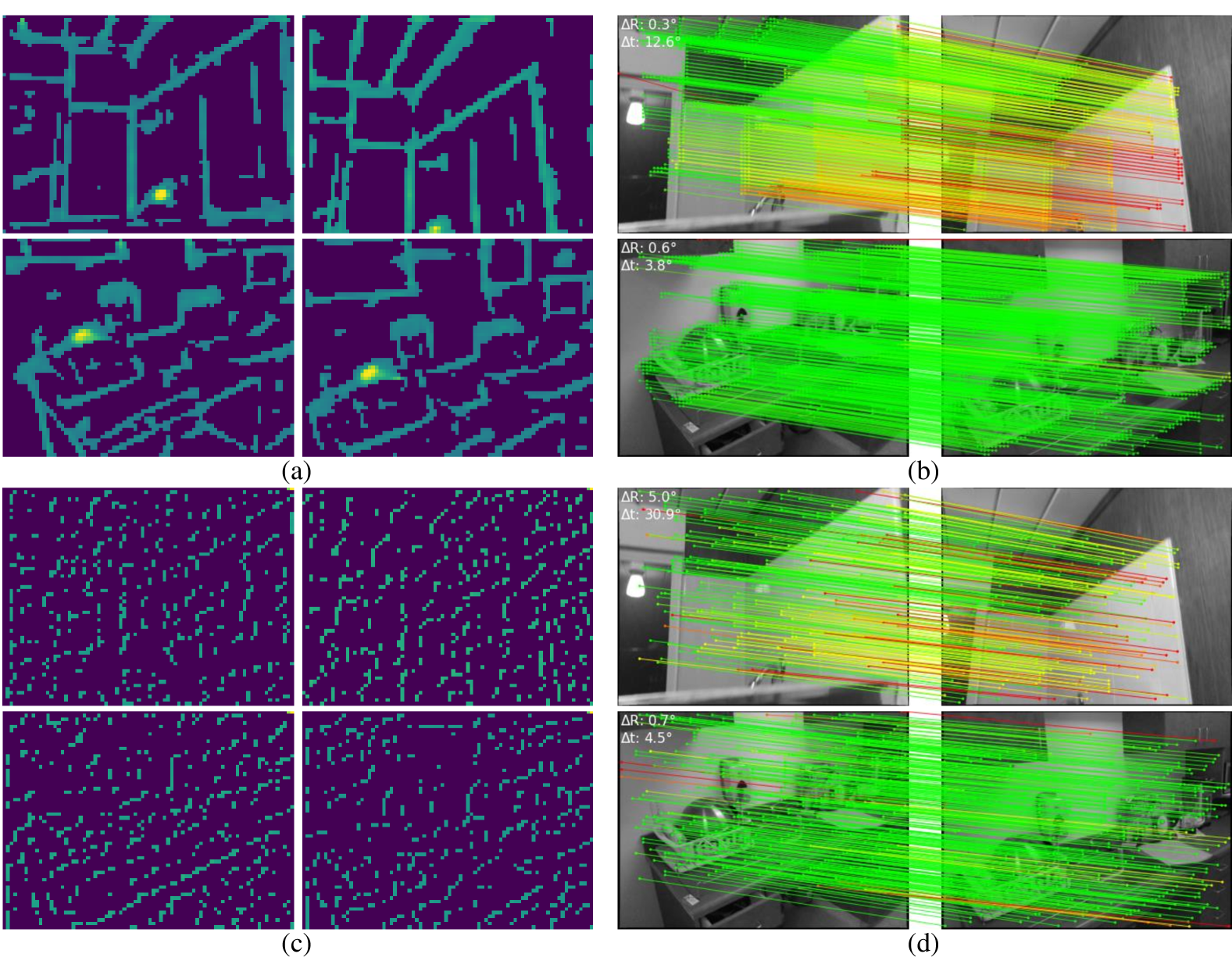
Figure 5: Matching results of sparse LoFTR. (a) and (b) present the score maps and matching results for an average feature proportion of 0.22. (c) and (d) are the score maps and matching results for an average feature proportion of 0.11. In the score maps, the lighter sections represent the features retained after pruning. When the proportion of retained features is higher, the score head behaves like edge detector. When the proportion is lower, the score head behaves like point detector.

5 Conclusion

This paper presents a novel reweighting method, which is applicable to a wide range of Transformer-based matching networks and adapts them to different sparsity levels without altering network parameters. We prove that the reweighted matching network can be viewed as the asymptotic limit of detector-based matching network, leading to consistency in feature importance and aiding generalization to dense features. Experiments show that the reweighting method can improve pose accuracy of detector-based matcher and enhance adaptability of detector-free matcher. Furthermore, our method provides a novel perspective for evaluating mainstream matching networks by transferring them to comparable sparsity levels before evaluation. This enables a better comparison by mitigating the impact of information disparity caused by differences in sparsity, thereby facilitating the future design of adaptive matchers.

Supplementary Material

6 Proofs to theorems

In Theorem 1, we demonstrate the asymptotic equivalence of the reweighted Transformer and the original Transformer. To prove this asymptotic equivalence, we first introduce and prove a theorem concerning the asymptotic equivalence of single attention layer. Then we prove Theorem 1 for Transformers of arbitrary depth. Similarly, Theorem 2 can be proved using analogous techniques.

6.1 Proof of asymptotic equivalence of reweighted attention layer

Theorem 3.

Given tokens $\mathbf{Q}^{*}$, $\mathbf{K}^{*}$ and $\mathbf{V}^{*}$, and an attention layer described in Sec. 3.2, $\mathbf{Q}^{*}\in\mathbb{R}^{d\times n^{*}},\mathbf{K}^{*}\in\mathbb{R}^{d\times m^{*}},\mathbf{V}^{*}\in\mathbb{R}^{d\times m^{*}}$. Denote $\{1,\ldots,n\}$ as $[n]$. For $m,n\in\mathbb{N}^{+}$, which approach infinity, suppose there are sequences of randomly expanding tokens $\mathbf{Q}^{(n)}$, $\mathbf{K}^{(m)}$ and $\mathbf{V}^{(m)}$ that satisfy:

(a) The tokens grow with the numbers of samples $m,n$:

$$\mathbf{Q}^{(n)}\in\mathbb{R}^{d\times n},\mathbf{K}^{(m)},\mathbf{V}^{(m)}\in\mathbb{R}^{d\times m}.$$ (14)

(b) The $j$-th token of $\mathbf{Q}^{(n)}$ converges in probability to $\mathbf{Q}_{j^{*}}^{*}$:

$$\forall j\in\mathbb{N}^{+},\exists j^{*}\in[n^{*}]:\mathbf{Q}_{j}^{(n)}\xrightarrow{P}\mathbf{Q}_{j^{*}}^{*}.$$ (15)

(c) The sampling of $\mathbf{K}^{(n)}$ and $\mathbf{V}^{(n)}$ is synchronous:

$$\begin{split}&\forall i\in\mathbb{N}^{+},\exists i^{*}\in[m^{*}]:\\ &\mathbf{K}_{i}^{(m)}\xrightarrow{P}\mathbf{K}_{i^{*}}^{*},\mathbf{V}_{i}^{(m)}\xrightarrow{P}\mathbf{V}_{i^{*}}^{*}.\end{split}$$ (16)

(d) For index sets $\mathcal{I}_{m}(i^{*})=\{k|k\in[m],k^{*}=i^{*}\}$, the tokens satisfy:

$$\begin{split}&\forall i^{*}\in[m^{*}],\forall i,i^{\prime}\in\mathcal{I}_{m}(i^{*}):\\ &\mathbf{K}_{i}^{(m)}=\mathbf{K}_{i^{\prime}}^{(m)},\mathbf{V}_{i}^{(m)}=\mathbf{V}_{i^{\prime}}^{(m)},\\ &\frac{1}{m}\left\lvert\mathcal{I}_{m}(i^{*})\right\rvert\xrightarrow{P}p(i^{*}),\end{split}$$ (17)

where $p(i^{*})$ is the probability associated with $\mathbf{K}_{i^{*}}^{*}$ and $\mathbf{V}_{i^{*}}^{*}$.

Let $\mathbf{Q}^{{}^{\prime}(m,n)}$ be the updated token of the attention layer, with $\mathbf{Q}^{(n)}$, $\mathbf{K}^{(m)}$ and $\mathbf{V}^{(m)}$ as input. And let $\mathbf{Q}^{{}^{\prime}*}$ represent the updated token of the reweighted attention layer, which replaces $\mathrm{Sim}$ with $\mathrm{Sim}^{p}$ in Eq. 6, and takes $\mathbf{Q}^{*}$, $\mathbf{K}^{*}$ and $\mathbf{V}^{*}$ as input. Then for any $j\in\mathbb{N}^{+}$, as $m,n$ approach infinity, we have

$$\mathbf{Q}_{j}^{{}^{\prime}(m,n)}\stackrel{{\scriptstyle P}}{{\longrightarrow}}\mathbf{Q}^{{}^{\prime}*}_{j^{*}}.$$ (18)

Proof.

For fixed $m,n$, we omit the superscripts with them and rewrite the computation of the attention layer as follows:

$$\begin{split}&\mathbf{Y}=\mathbf{Q}+\sum_{h=1}^{H}\mathbf{W}_{VO}^{h}\mathbf{V}\mathrm{Sim}(\mathbf{W}_{K}^{h}\mathbf{K},\mathbf{W}_{Q}^{h}\mathbf{Q})\\ &\mathbf{Q}^{\prime}=\mathbf{Y}+\mathbf{W}_{2}\mathrm{Act}(\mathbf{W}_{1}\mathbf{Y}+\mathbf{b}_{1}\mathbf{1}^{\top})+\mathbf{b}_{2}\mathbf{1}^{\top},\end{split}$$ (19)

where $H$ is the number of attention heads, and $\mathbf{W}_{VO}^{h}$, $\mathbf{W}_{K}^{h}$, and $\mathbf{W}_{Q}^{h}$ are parameter matrices of the $h$-th attention head. The $\mathbf{W}_{1},\mathbf{W}_{2}$ and $\mathbf{b}_{1},\mathbf{b}_{2}$ are parameter matrices and vectors of the feed forward part.

Denote the result of the $h$-th attention head as $\mathbf{Y}^{h}$, and denote the result of the $h$-th reweighted attention head as $\mathbf{Y}^{h*}$:

$$\begin{split}&\mathbf{Y}^{h}=\mathbf{W}_{VO}^{h}\mathbf{V}\mathrm{Sim}(\mathbf{W}_{K}^{h}\mathbf{K},\mathbf{W}_{Q}^{h}\mathbf{Q})\\ &\mathbf{Y}^{h*}=\mathbf{W}_{VO}^{h}\mathbf{V}^{*}\mathrm{Sim}^{p}(\mathbf{W}_{K}^{h}\mathbf{K}^{*},\mathbf{W}_{Q}^{h}\mathbf{Q}^{*}).\end{split}$$ (20)

For $i\in[m],j\in[n]$, denote $s_{i,j}$ as $\delta(\mathbf{W}_{K}^{h}\mathbf{K}_{i},\mathbf{W}_{Q}^{h}\mathbf{Q}_{j})$, and for $i^{*}\in[m^{*}]$, $j^{*}\in[n^{*}]$, denote $s^{*}_{i^{*},j^{*}}$ as $\delta(\mathbf{W}_{K}^{h}\mathbf{K}^{*}_{i^{*}},\mathbf{W}_{Q}^{h}\mathbf{Q}^{*}_{j^{*}})$. We have

$$\mathbf{Y}_{j}^{h} =\mathbf{W}_{VO}^{h}\mathbf{V}\cdot\frac{1}{\sum\limits_{i=1}^{m}{s_{i,j}}}\left[\begin{matrix}{{s}_{1,j}}\\ {{s}_{2,j}}\\ \vdots\\ {{s}_{{m},j}}\\ \end{matrix}\right]$$ (21)

$$={{\mathbf{W}}_{VO}^{h}}\cdot\frac{1}{\sum\limits_{i=1}^{{m}}{{{s}_{i,j}}}}\sum\limits_{i=1}^{{m}}{{{s}_{i,j}}{{\mathbf{V}}_{i}}}$$

$$={{\mathbf{W}}_{VO}^{h}}\cdot\frac{1}{\frac{1}{{m}}\sum\limits_{i=1}^{{m}}{{{s}_{i,j}}}}\cdot\frac{1}{{m}}\sum\limits_{i=1}^{{m}}{{{s}_{i,j}}{{\mathbf{V}}_{i}}}.$$

When $m,n$ approaches infinity, we have

$$\frac{1}{m}\sum\limits_{i=1}^{m}{{{s}_{i,j}}} =\sum\limits_{{{i}^{*}}=1}^{{{m}^{*}}}\frac{\left|{{\mathcal{I}}_{m}}({{i}^{*}})\right|}{m}$$ (22)

$$\cdot\frac{1}{\left|{{\mathcal{I}}_{m}}({{i}^{*}})\right|}\sum\limits_{i\in{{\mathcal{I}}_{m}}({{i}^{*}})}{\delta(\mathbf{W}_{K}^{h}\mathbf{K}_{i}^{(m)},\mathbf{W}_{Q}^{h}\mathbf{Q}_{j}^{(n)})}$$

$$\xrightarrow{P}\sum\limits_{{{i}^{*}}=1}^{{{m}^{*}}}{p({{i}^{*}})\delta(\mathbf{W}_{K}^{h}\mathbf{K}_{{{i}^{*}}}^{*},\mathbf{W}_{Q}^{h}\mathbf{Q}_{{{j}^{*}}}^{*})}$$

$$=\sum\limits_{{{i}^{*}}=1}^{{{m}^{*}}}{p({{i}^{*}})s_{{{i}^{*}},{{j}^{*}}}^{*}},$$

and

$$\frac{1}{m}\sum\limits_{i=1}^{m}{{{s}_{i,j}}}{{\mathbf{V}}_{i}^{(m)}}\xrightarrow{P}\sum\limits_{{{i}^{*}}=1}^{{{m}^{*}}}{p({{i}^{*}})s_{{{i}^{*}},{{j}^{*}}}^{*}}{{\mathbf{V}}_{i^{*}}^{*}}.$$ (23)

Substitute Eqs. 22 and 23 into Eq. 21, we have

$$\mathbf{Y}_{j}^{h(m,n)} \xrightarrow{P}{{\mathbf{W}}_{VO}^{h}}\cdot\frac{1}{\sum\limits_{{{i}^{*}}=1}^{m^{*}}{p({{i}^{*}})s_{{{i}^{*}},{{j}^{*}}}^{*}}}\sum\limits_{{{i}^{*}}=1}^{m^{*}}{p({{i}^{*}})s_{{{i}^{*}},{{j}^{*}}}^{*}}\mathbf{V}_{{{i}^{*}}}^{*}$$ (24)

$$={{\mathbf{W}}_{VO}^{h}}\mathbf{V}^{*}\cdot\frac{1}{\sum\limits_{{{i}^{*}}=1}^{m^{*}}{p({{i}^{*}})s_{{{i}^{*}},{{j}^{*}}}^{*}}}\left[\begin{matrix}p(1){{s}_{1,j^{*}}^{*}}\\ p(2){{s}_{2,j^{*}}^{*}}\\ \vdots\\ p({m^{*}}){{s}_{{m^{*}},j^{*}}^{*}}\\ \end{matrix}\right]$$

$$=\mathbf{Y}_{j^{*}}^{h*}.$$

Therefore, we have

$$\mathbf{Y}_{j}^{(m,n)} =\mathbf{Q}_{j}^{(n)}+\sum_{h=1}^{H}\mathbf{Y}_{j}^{h(m,n)}$$ (25)

$$\xrightarrow{P}\mathbf{Q^{*}}_{j^{*}}+\sum_{h=1}^{H}\mathbf{Y}_{j^{*}}^{h*}$$

$$=\mathbf{Y}^{*}_{j}\text{.}$$

Because the feed forward part is continuous element-wise function, we obtain

$$\begin{split}\mathbf{Q}_{j}^{{}^{\prime}(m,n)}&=\mathbf{Y}_{j}^{(m,n)}+\mathbf{W}_{2}\mathrm{Act}(\mathbf{W}_{1}\mathbf{Y}_{j}^{(m,n)}+\mathbf{b}_{1}\mathbf{1}^{\top})+\mathbf{b}_{2}\mathbf{1}^{\top}\\ &\xrightarrow{P}\mathbf{Y}^{*}_{j^{*}}+\mathbf{W}_{2}\mathrm{Act}(\mathbf{W}_{1}\mathbf{Y}^{*}_{j^{*}}+\mathbf{b}_{1}\mathbf{1}^{\top})+\mathbf{b}_{2}\mathbf{1}^{\top}\\ &=\mathbf{Q}^{{}^{\prime}*}_{j^{*}}.\end{split}$$ (26)

∎

6.2 Proof of Theorem 1

Proof.

As described in Sec. 3.1, feature points $F_{A}$ and $F^{\prime}_{A}$ only differ in feature descriptors, keeping points coordinates unchanged. Therefore, we only need to examine the convergence values of the updated feature descriptors, namely, the output tokens of the network. We first examine the outputs of the embedding layer. Then we employ mathematical induction on the depth of the Transformers $\mathrm{TF}$ and $\mathrm{TF}^{p_{A},p_{B}}$.

The embedding layer is the first layer of the Transformer, and it is point-wise, which aligns with mainstream designs like rotary position embedding. Thus, the embedding of each feature point is not influenced by other feature points. Let the size of $F_{A}$ and $F_{A}^{*}$ be $n_{A}$ and $n_{A}^{*}$, respectively. As described in Sec. 3.1, $F_{A}$ are i.i.d. samples of $F_{A}^{*}$, and for any index $i,1\leq i\leq n_{A}$ and its corresponding index $i^{*},1\leq i^{*}\leq n_{A}^{*}$, we have $F_{A,i}=F_{A,i^{*}}^{*}$. Denote the resulting tokens from the embedding layer of $F_{A}$ and $F_{A}^{*}$ as $\mathbf{X}_{A}$ and $\mathbf{X}_{A}^{*}$, respectively. Because we don’t reweight the point-wise embedding layer, we have $\mathbf{X}_{A,i}=\mathbf{X}_{A,i^{*}}^{*}$. Similarly, $\mathbf{X}_{B,j}=\mathbf{X}_{B,j^{*}}^{*},1\leq j\leq n_{B},1\leq j^{*}\leq n_{B}^{*}$.

The attention layers aggregates input tokens. Let the number of attention layers in $\mathrm{TF}$ be $l$. Denote the input tokens of the $l$-th attention layer in $\mathrm{TF}$ as $\mathbf{X}_{Q}$, $\mathbf{X}_{K}$, and $\mathbf{X}_{V}$. Similarly, the input tokens of the $l$-th reweighted attention layer in $\mathrm{TF}^{p_{A},p_{B}}$ are denoted as $\mathbf{X}_{Q}^{*}$, $\mathbf{X}_{K}^{*}$ and $\mathbf{X}_{V}^{*}$. In a typical Transformer design, we have $\mathbf{X}_{K}=\mathbf{X}_{V}$ and $\mathbf{X}_{K}^{*}=\mathbf{X}_{V}^{*}$. Thus, Eq. 14 is satisfied. According to the law of large numbers, Eq. 17 is satisfied.

When $l=1$, $\mathrm{TF}$ consists of one embedding layer and one attention layer. We have $\mathbf{X}_{Q},\mathbf{X}_{K},\mathbf{X}_{V}\in\left\{\mathbf{X}_{A},\mathbf{X}_{B}\right\}$, and the exact assignment depends on the design choice of the layer. According to the discussion on the embedding layer, Eqs. 15 and 16 hold true. Applying Theorem 3, we obtain that the output tokens of $\mathrm{TF}$ converge in probability to the output tokens of $\mathrm{TF}^{p_{A},p_{B}}$.

When $l>1$, applying mathematical induction on Transformers with $l-1$ attention layers, Eqs. 15 and 16 are satisfied. Again, applying Theorem 3, Theorem 1 is proved.

∎

6.3 Proof of Theorem 2

Proof.

Original optimal transport in image matching assigns equal weights to the points to be matched:

$${{\mathbf{a}}_{i}}=\frac{1}{{{n}_{A}}},{{\mathbf{a}}_{{{n}_{A}}+1}}=1,1\leq i\leq{{n}_{A}}$$ (27)

$${{\mathbf{b}}_{j}}=\frac{1}{{{n}_{B}}},{{\mathbf{b}}_{{{n}_{B}}+1}}=1,1\leq j\leq{{n}_{B}},$$

where ${n}_{A},{n}_{B}$ are numbers of sampled features of image $A$ and $B$ which tend to infinity.

Reweighted optimal transport employs feature detection probabilities ${p}_{A}$ and ${p}_{B}$ for the weights:

$$\mathbf{a}_{{{i}^{*}}}^{*}={{p}_{A}}({{i}^{*}}),\mathbf{a}_{n_{A}^{*}+1}^{*}=1,1\leq{{i}^{*}}\leq n_{A}^{*}$$ (28)

$$\mathbf{b}_{{{j}^{*}}}^{*}={{p}_{B}}({{j}^{*}}),\mathbf{b}_{n_{B}^{*}+1}^{*}=1,1\leq{{j}^{*}}\leq n_{B}^{*},$$

where $n_{A}^{*},n_{B}^{*}$ represents the total numbers of features in the feature maps of $A$ and $B$.

Denote the score matrices of original matching and reweighted matching as $\overline{\mathbf{S}}$ and $\overline{\mathbf{S}}^{*}$, respectively. According to Theorem 1, the scores converge in probability:

$$\begin{split}&\forall i\in[n_{A}],\forall j\in[n_{B}],\exists{{i}^{*}}\in[n_{A}^{*}],\exists{{j}^{*}}\in[n_{B}^{*}]:\\ &{{\overline{\mathbf{S}}}_{i,j}}\xrightarrow{P}\overline{\mathbf{S}}_{{{i}^{*}},{{j}^{*}}}^{*}\end{split}$$ (29)

Because we do not change the dustbin score, the elements in the last rows or the last columns of $\overline{\mathbf{S}}$ and $\overline{\mathbf{S}}^{*}$ equal to the dustbin score $\alpha$.

Define ${{\mathcal{I}}_{{{n}_{A}}}}({{i}^{*}})=\{k|k\in[{{n}_{A}}],{{k}^{*}}={{i}^{*}}\}$, ${{\mathcal{J}}_{{{n}_{B}}}}({{j}^{*}})=\{l|l\in[{{n}_{B}}],{{l}^{*}}={{j}^{*}}\}$. We have

$$\forall{{i}^{*}}\in[n_{A}^{*}],\forall{{j}^{*}}\in[n_{B}^{*}],\forall i,{i}^{\prime} \in{{\mathcal{I}}_{{{n}_{A}}}}({{i}^{*}}),\forall j,{j}^{\prime}\in{{\mathcal{J}}_{{{n}_{B}}}}({{j}^{*}}):$$ (30)

$${{\overline{\mathbf{S}}}_{i,j}} ={{\overline{\mathbf{S}}}_{{i}^{\prime},{j}^{\prime}}},$$

$$\frac{1}{{{n}_{A}}}\left|{{\mathcal{I}}_{{{n}_{A}}}}({{i}^{*}})\right| \xrightarrow{P}{{p}_{A}}({{i}^{*}}),$$

$$\frac{1}{{{n}_{B}}}\left|{{\mathcal{J}}_{{{n}_{B}}}}({{j}^{*}})\right| \xrightarrow{P}{{p}_{B}}({{j}^{*}}).$$

In original matching, sinkhorn algorithm computes the output assignment as

$$\text{OT}_{i,j}={{\mathbf{u}}_{i}}{{\mathbf{K}}_{i,j}}{{\mathbf{v}}_{j}}.$$ (31)

Each iteration of the algorithm updates vectors $\mathbf{u},\mathbf{v}$ to $\mathbf{{u}^{\prime}},\mathbf{{v}^{\prime}}$:

$${{\mathbf{{u}^{\prime}}}_{i}}=\frac{{{\mathbf{a}}_{i}}}{{{(\mathbf{Kv})}_{i}}},{{\mathbf{{v}^{\prime}}}_{j}}=\frac{{{\mathbf{b}}_{j}}}{{{({{\mathbf{K}}^{\top}}\mathbf{{u}^{\prime}})}_{j}}},$$ (32)

where ${{\mathbf{K}}_{i,j}}={\mathrm{exp}({\frac{{{\overline{\mathbf{S}}}_{i,j}}}{\varepsilon}}})$.

In reweighted matching, the same algorithm computes the output assignment

$$\text{OT}_{{{i}^{*}},{{j}^{*}}}^{{{p}_{A}},{{p}_{B}}}=\mathbf{u}_{{{i}^{*}}}^{*}\mathbf{K}_{{{i}^{*}},{{j}^{*}}}^{*}\mathbf{v}_{{{j}^{*}}}^{*}.$$ (33)

Each iteration updates vector ${\mathbf{{u}}}^{*},{\mathbf{{v}}}^{*}$ to ${\mathbf{{u}^{\prime}}}^{*},{\mathbf{{v}^{\prime}}}^{*}$:

$${\mathbf{{u}^{\prime}}}^{*}_{{{i}^{*}}}=\frac{\mathbf{a}_{{{i}^{*}}}^{*}}{{{({{\mathbf{K}}^{*}}{{\mathbf{v}}^{*}})}_{{{i}^{*}}}}},{\mathbf{{v}^{\prime}}}^{*}_{{{j}^{*}}}=\frac{\mathbf{b}_{{{j}^{*}}}^{*}}{{{({{\mathbf{K}}^{*}}^{\top}{{{\mathbf{{u}^{\prime}}}}^{*}})}_{{{j}^{*}}}}},$$ (34)

where ${{\mathbf{K}}_{i^{*},j^{*}}^{*}}={\mathrm{exp}({\frac{{{\overline{\mathbf{S}}}_{i^{*},j^{*}}^{*}}}{\varepsilon}}})$.

At the first iteration, $\mathbf{u},\mathbf{v},{\mathbf{{u}}}^{*},{\mathbf{{v}}}^{*}$ can be initialized with arbitrary positive vectors. For simplicity, we initialize $\mathbf{u},\mathbf{v},{\mathbf{{u}}}^{*},{\mathbf{{v}}}^{*}$ as $\mathbf{a},\mathbf{b},\mathbf{a}^{*},\mathbf{b}^{*}$, respectively. Thus, the initialized values satisfy $n_{A}\mathbf{u}_{i}=p_{A}(i^{*})^{-1}\mathbf{u}_{i^{*}}^{*}$, $n_{B}\mathbf{v}_{j}=p_{B}(j^{*})^{-1}\mathbf{v}_{j^{*}}^{*}$, $i\in[n_{A}],j\in[n_{B}]$, and $\mathbf{u}_{n_{A}+1}=\mathbf{u}^{*}_{n_{A}^{*}+1}=\mathbf{v}_{n_{B}+1}=\mathbf{v}^{*}_{n_{B}^{*}+1}=1$. Now we employ mathematical induction, and assume that for the $l$-th iteration:

$$\begin{split}n_{A}\mathbf{u}_{i}&\xrightarrow{P}p_{A}(i^{*})^{-1}\mathbf{u}_{i^{*}}^{*},i\in[n_{A}],\\ n_{B}\mathbf{v}_{j}&\xrightarrow{P}p_{B}(j^{*})^{-1}\mathbf{v}_{j^{*}}^{*},j\in[n_{B}],\\ \mathbf{u}_{n_{A}+1}&\xrightarrow{P}\mathbf{u}^{*}_{n_{A}^{*}+1},\\ \mathbf{v}_{n_{B}+1}&\xrightarrow{P}\mathbf{v}^{*}_{n_{B}^{*}+1}.\end{split}$$ (35)

Then for $i\in[n_{A}],j\in[n_{B}]$, we have

$${{n}_{A}}{{{\mathbf{{u}^{\prime}}}}_{i}} ={{(\mathbf{Kv})}_{i}}^{-1}$$ (36)

$$={{\left(\alpha\mathbf{v}_{n_{B}+1}+\sum\limits_{j=1}^{{{n}_{B}}}{{{\mathbf{K}}_{i,j}}{{\mathbf{v}}_{j}}}\right)}^{-1}}$$

$$={{\left(\alpha\mathbf{v}_{n_{B}+1}+\sum\limits_{{{j}^{*}}=1}^{n_{B}^{*}}{\frac{1}{{{n}_{B}}}}\sum\limits_{j\in{{\mathcal{J}}_{{{n}_{B}}}}({{j}^{*}})}{{{\mathbf{K}}_{i,j}}\cdot({{n}_{B}}{{\mathbf{v}}_{j}})}\right)}^{-1}}$$

$$\xrightarrow{P}{{\left(\alpha\mathbf{v}_{n_{B}^{*}+1}^{*}+\sum\limits_{{{j}^{*}}=1}^{n_{B}^{*}}{{{p}_{B}}({{j}^{*}})}\mathbf{K}_{{{i}^{*}},{{j}^{*}}}^{*}\cdot{{p}_{B}}{{({{j}^{*}})}^{-1}}\mathbf{v}_{{{j}^{*}}}^{*}\right)}^{-1}}$$

$$={{({{\mathbf{K}}^{*}}{{\mathbf{v}}^{*}})}_{{{i}^{*}}}}^{-1}$$

$$={{p}_{A}}{{({{i}^{*}})}^{-1}}\mathbf{{u}^{\prime}}_{{{i}^{*}}}^{*}$$

$${{n}_{B}}{{{\mathbf{{v}^{\prime}}}}_{j}} ={{({{\mathbf{K}}^{\top}}\mathbf{{u}^{\prime}})}_{j}}^{-1}$$ (37)

$$={{\left(\alpha\mathbf{u^{\prime}}_{n_{A}+1}+\sum\limits_{i=1}^{{{n}_{A}}}{{{\mathbf{K}}_{i,j}}{{{\mathbf{{u}^{\prime}}}}_{i}}}\right)}^{-1}}$$

$$={{\left(\alpha\mathbf{u^{\prime}}_{n_{A}+1}+\sum\limits_{{{i}^{*}}=1}^{n_{A}^{*}}{\frac{1}{{{n}_{A}}}}\sum\limits_{i\in{{\mathcal{I}}_{{{n}_{A}}}}({{i}^{*}})}{{{\mathbf{K}}_{i,j}}({{n}_{A}}{{{\mathbf{{u}^{\prime}}}}_{i}})}\right)}^{-1}}$$

$$\xrightarrow{P}{{\left(\alpha\mathbf{u^{\prime}}_{n_{A}^{*}+1}^{*}+\sum\limits_{{{i}^{*}}=1}^{n_{A}^{*}}{{{p}_{A}}({{i}^{*}})}\mathbf{K}_{{{i}^{*}},{{j}^{*}}}^{*}\cdot{{p}_{A}}{{({{i}^{*}})}^{-1}}\mathbf{{u}^{\prime}}_{{{i}^{*}}}^{*}\right)}^{-1}}$$

$$={{p}_{B}}{{({{j}^{*}})}^{-1}}{{\mathbf{{v}^{\prime}}}}^{*}_{{{j}^{*}}}$$

Similarly, we obtain $\mathbf{u^{\prime}}_{n_{A}+1}\xrightarrow{P}\mathbf{u^{\prime}}^{*}_{n_{A}^{*}+1}$ and $\mathbf{v^{\prime}}_{n_{B}+1}\xrightarrow{P}\mathbf{v^{\prime}}^{*}_{n_{B}^{*}+1}$.

Therefore, Eq. 35 holds in all iterations and in Eqs. 31 and 33. For each $i^{*},j^{*}$, by summing up all $\text{OT}_{i,j}$ within ${\mathcal{I}}_{{{n}_{A}}}({{i}^{*}})$ and ${{\mathcal{J}}_{{{n}_{B}}}}({{j}^{*}})$, and examining the convergence value in terms of probability, we prove the validity of Theorem 2 in the context of optimal transport. The validity about matching using dual-softmax can also be proved using analogous techniques. ∎

References

- Barroso-Laguna et al. [2024] Axel Barroso-Laguna, Sowmya Munukutla, Victor Adrian Prisacariu, and Eric Brachmann. Matching 2D Images in 3D: Metric Relative Pose from Metric Correspondences. In Proceedings of the IEEE/CVF Conference on Computer Vision and Pattern Recognition, pages 4852–4863, 2024.
- Bay et al. [2006] Herbert Bay, Tinne Tuytelaars, and Luc Van Gool. SURF: Speeded Up Robust Features. In Computer Vision – ECCV 2006, pages 404–417, Berlin, Heidelberg, 2006. Springer.
- Chen et al. [2020] Changhao Chen, Bing Wang, Chris Xiaoxuan Lu, Niki Trigoni, and Andrew Markham. A survey on deep learning for localization and mapping: Towards the age of spatial machine intelligence. arXiv preprint arXiv:2006.12567, 2020.
- Chen et al. [2021] Hongkai Chen, Zixin Luo, Jiahui Zhang, Lei Zhou, Xuyang Bai, Zeyu Hu, Chiew-Lan Tai, and Long Quan. Learning to match features with seeded graph matching network. In Proceedings of the IEEE/CVF International Conference on Computer Vision, pages 6301–6310, 2021.
- Chen et al. [2022] Hongkai Chen, Zixin Luo, Lei Zhou, Yurun Tian, Mingmin Zhen, Tian Fang, David McKinnon, Yanghai Tsin, and Long Quan. ASpanFormer: Detector-Free Image Matching with Adaptive Span Transformer. In Computer Vision – ECCV 2022, pages 20–36. Springer Nature Switzerland, Cham, 2022.
- Choy et al. [2016] Christopher B. Choy, JunYoung Gwak, Silvio Savarese, and Manmohan Chandraker. Universal correspondence network. Advances in neural information processing systems, 29, 2016.
- Cuturi [2013] Marco Cuturi. Sinkhorn distances: Lightspeed computation of optimal transport. Advances in neural information processing systems, 26, 2013.
- Dai et al. [2017] Angela Dai, Angel X. Chang, Manolis Savva, Maciej Halber, Thomas Funkhouser, and Matthias Nießner. ScanNet: Richly-Annotated 3D Reconstructions of Indoor Scenes. In 2017 IEEE Conference on Computer Vision and Pattern Recognition (CVPR), pages 2432–2443, 2017.
- DeTone et al. [2018] Daniel DeTone, Tomasz Malisiewicz, and Andrew Rabinovich. SuperPoint: Self-Supervised Interest Point Detection and Description. In 2018 IEEE/CVF Conference on Computer Vision and Pattern Recognition Workshops (CVPRW), pages 337–33712, 2018.
- Dusmanu et al. [2019] Mihai Dusmanu, Ignacio Rocco, Tomas Pajdla, Marc Pollefeys, Josef Sivic, Akihiko Torii, and Torsten Sattler. D2-Net: A Trainable CNN for Joint Description and Detection of Local Features. In 2019 IEEE/CVF Conference on Computer Vision and Pattern Recognition (CVPR), pages 8084–8093, 2019.
- Edstedt et al. [2023] Johan Edstedt, Ioannis Athanasiadis, Mårten Wadenbäck, and Michael Felsberg. DKM: Dense kernelized feature matching for geometry estimation. In Proceedings of the IEEE/CVF Conference on Computer Vision and Pattern Recognition, pages 17765–17775, 2023.
- Edstedt et al. [2024] Johan Edstedt, Qiyu Sun, Georg Bökman, Mårten Wadenbäck, and Michael Felsberg. RoMa: Robust dense feature matching. In Proceedings of the IEEE/CVF Conference on Computer Vision and Pattern Recognition, pages 19790–19800, 2024.
- Fischler and Bolles [1981] Martin A. Fischler and Robert C. Bolles. Survey on deep learningsample consensus: A paradigm for model fitting with applications to image analysis and automated cartography. Communications of the ACM, 24(6):381–395, 1981.
- Harris and Stephens [1988] Chris Harris and Mike Stephens. A combined corner and edge detector. In Alvey Vision Conference, pages 10–5244. Citeseer, 1988.
- Li et al. [2022] Kunhong Li, Longguang Wang, Li Liu, Qing Ran, Kai Xu, and Yulan Guo. Decoupling makes weakly supervised local feature better. In Proceedings of the IEEE/CVF Conference on Computer Vision and Pattern Recognition, pages 15838–15848, 2022.
- Li et al. [2020] Xinghui Li, Kai Han, Shuda Li, and Victor Prisacariu. Dual-resolution correspondence networks. Advances in Neural Information Processing Systems, 33:17346–17357, 2020.
- Li and Snavely [2018] Zhengqi Li and Noah Snavely. Megadepth: Learning single-view depth prediction from internet photos. In Proceedings of the IEEE Conference on Computer Vision and Pattern Recognition, pages 2041–2050, 2018.
- Lindenberger et al. [2023] Philipp Lindenberger, Paul-Edouard Sarlin, and Marc Pollefeys. Lightglue: Local feature matching at light speed. In Proceedings of the IEEE/CVF International Conference on Computer Vision, pages 17627–17638, 2023.
- Liu et al. [2010] Ce Liu, Jenny Yuen, and Antonio Torralba. Sift flow: Dense correspondence across scenes and its applications. IEEE transactions on pattern analysis and machine intelligence, 33(5):978–994, 2010.
- Lowe [2004] D. G. Lowe. Distinctive Image Features from Scale-Invariant Keypoints. International Journal of Computer Vision, 60(2):91–110, 2004.
- Lynen et al. [2020] Simon Lynen, Bernhard Zeisl, Dror Aiger, Michael Bosse, Joel Hesch, Marc Pollefeys, Roland Siegwart, and Torsten Sattler. Large-scale, real-time visual–inertial localization revisited. The International Journal of Robotics Research, 39(9):1061–1084, 2020.
- Ni et al. [2023] Junjie Ni, Yijin Li, Zhaoyang Huang, Hongsheng Li, Hujun Bao, Zhaopeng Cui, and Guofeng Zhang. Pats: Patch area transportation with subdivision for local feature matching. In Proceedings of the IEEE/CVF Conference on Computer Vision and Pattern Recognition, pages 17776–17786, 2023.
- Revaud et al. [2019] Jerome Revaud, Cesar De Souza, Martin Humenberger, and Philippe Weinzaepfel. R2d2: Reliable and repeatable detector and descriptor. Advances in neural information processing systems, 32, 2019.
- Rocco et al. [2022] Ignacio Rocco, Mircea Cimpoi, Relja Arandjelović, Akihiko Torii, Tomas Pajdla, and Josef Sivic. NCNet: Neighbourhood Consensus Networks for Estimating Image Correspondences. IEEE Transactions on Pattern Analysis and Machine Intelligence, 44(2):1020–1034, 2022.
- Rublee et al. [2011] Ethan Rublee, Vincent Rabaud, Kurt Konolige, and Gary R. Bradski. ORB: An efficient alternative to SIFT or SURF. In IEEE International Conference on Computer Vision, ICCV 2011, Barcelona, Spain, November 6-13, 2011, 2011.
- Sarlin et al. [2019] Paul-Edouard Sarlin, Cesar Cadena, Roland Siegwart, and Marcin Dymczyk. From coarse to fine: Robust hierarchical localization at large scale. In Proceedings of the IEEE/CVF Conference on Computer Vision and Pattern Recognition, pages 12716–12725, 2019.
- Sarlin et al. [2020] Paul-Edouard Sarlin, Daniel DeTone, Tomasz Malisiewicz, and Andrew Rabinovich. SuperGlue: Learning Feature Matching With Graph Neural Networks. In Proceedings of the IEEE/CVF Conference on Computer Vision and Pattern Recognition, pages 4938–4947, 2020.
- Schmidt et al. [2017] Tanner Schmidt, Richard Newcombe, and Dieter Fox. Self-Supervised Visual Descriptor Learning for Dense Correspondence. IEEE Robotics and Automation Letters, 2(2):420–427, 2017.
- Schonberger and Frahm [2016] Johannes L. Schonberger and Jan-Michael Frahm. Structure-from-motion revisited. In Proceedings of the IEEE Conference on Computer Vision and Pattern Recognition, pages 4104–4113, 2016.
- Shi et al. [2022] Yan Shi, Jun-Xiong Cai, Yoli Shavit, Tai-Jiang Mu, Wensen Feng, and Kai Zhang. Clustergnn: Cluster-based coarse-to-fine graph neural network for efficient feature matching. In Proceedings of the IEEE/CVF Conference on Computer Vision and Pattern Recognition, pages 12517–12526, 2022.
- Sinkhorn and Knopp [1967] Richard Sinkhorn and Paul Knopp. Concerning nonnegative matrices and doubly stochastic matrices. Pacific Journal of Mathematics, 21(2):343–348, 1967.
- Sun et al. [2021] Jiaming Sun, Zehong Shen, Yuang Wang, Hujun Bao, and Xiaowei Zhou. LoFTR: Detector-Free Local Feature Matching with Transformers. In 2021 IEEE/CVF Conference on Computer Vision and Pattern Recognition (CVPR), pages 8918–8927, 2021.
- Taira et al. [2021] Hajime Taira, Masatoshi Okutomi, Torsten Sattler, Mircea Cimpoi, Marc Pollefeys, Josef Sivic, Tomas Pajdla, and Akihiko Torii. InLoc: Indoor Visual Localization with Dense Matching and View Synthesis. IEEE Transactions on Pattern Analysis and Machine Intelligence, 43(4):1293–1307, 2021.
- Truong et al. [2021] Prune Truong, Martin Danelljan, Luc Van Gool, and Radu Timofte. Learning accurate dense correspondences and when to trust them. In Proceedings of the IEEE/CVF Conference on Computer Vision and Pattern Recognition, pages 5714–5724, 2021.
- Tyszkiewicz et al. [2020] Michał Tyszkiewicz, Pascal Fua, and Eduard Trulls. DISK: Learning local features with policy gradient. Advances in Neural Information Processing Systems, 33:14254–14265, 2020.
- Vaswani et al. [2017] Ashish Vaswani, Noam Shazeer, Niki Parmar, Jakob Uszkoreit, Llion Jones, Aidan N Gomez, Łukasz Kaiser, and Illia Polosukhin. Attention is All you Need. In Advances in Neural Information Processing Systems. Curran Associates, Inc., 2017.
- Wang et al. [2022] Qing Wang, Jiaming Zhang, Kailun Yang, Kunyu Peng, and Rainer Stiefelhagen. Matchformer: Interleaving attention in transformers for feature matching. In Proceedings of the Asian Conference on Computer Vision, pages 2746–2762, 2022.
- Wang et al. [2024] Yifan Wang, Xingyi He, Sida Peng, Dongli Tan, and Xiaowei Zhou. Efficient LoFTR: Semi-dense local feature matching with sparse-like speed. In Proceedings of the IEEE/CVF Conference on Computer Vision and Pattern Recognition, pages 21666–21675, 2024.
- Zhang et al. [2021] Zichao Zhang, Torsten Sattler, and Davide Scaramuzza. Reference Pose Generation for Long-term Visual Localization via Learned Features and View Synthesis. International Journal of Computer Vision, 129(4):821–844, 2021.
- Zhu and Liu [2023] Shengjie Zhu and Xiaoming Liu. PMatch: Paired Masked Image Modeling for Dense Geometric Matching. In Proceedings of the IEEE/CVF Conference on Computer Vision and Pattern Recognition, pages 21909–21918, 2023.