Primordial black holes and scalar induced gravitational waves from sound speed resonance in derivatively coupling inflation model

Abstract

We study the amplification of primordial curvature perturbations through a sound speed resonance mechanism within an inflationary model featuring a non-minimal derivative coupling. In this scenario, the coupling function is composed of a constant term and a periodic term. Our analysis demonstrates that the periodic behavior of the squared sound speed transforms the curvature perturbation equation into a Mathieu equation on sub-horizon scales. This resonance effect leads to a substantial enhancement of curvature perturbations, which, upon re-entering the Hubble horizon during the radiation-dominated era, can trigger the formation of primordial black holes, potentially contributing to the dark matter density. Additionally, the amplified perturbations generate scalar-induced gravitational waves with amplitudes that may lie within the detectable range of future gravitational wave observatories, providing a testable observational signature of the model.

I Introduction

During the inflationary epoch, curvature perturbations are stretched beyond the Hubble radius and subsequently re-enter the horizon during the radiation- or matter-dominated eras. In regions where the density contrast is sufficiently high, gravitational collapse may occur, leading to the formation of primordial black holes (PBHs) Zeldovich ; Hawking ; Carr ; Meszaros ; Carr1975 ; Khlopov ; Ozsoy2023 . PBHs have garnered significant attention as they provide a plausible explanation for various astrophysical and cosmological phenomena, including the gravitational wave events observed by LIGO-Virgo lg1 ; lg2 ; lg3 ; lg4 , ultrashort microlensing events detected in OGLE data P.Mroz2017 ; H.Niikura2019 , and their potential role as a substantial component of dark matter, particularly in the asteroid-mass range A.Katz2018 ; A.Barnacka2012 ; P.W.Graham2015 ; H.Niikura2019a . Moreover, PBH formation is intrinsically linked to the presence of large scalar perturbations, which can also generate scalar-induced gravitational waves (SIGWs) yfcai2018 ; yfcai2019 that may be detectable by future gravitational wave observatories.

In order for PBHs to form abundantly, the power spectrum of curvature perturbations must achieve an amplitude of at least $\mathcal{O}(10^{-2})$. However, standard slow-roll inflation, as confirmed by observations of the cosmic microwave background (CMB) Aghanim2020 , predicts a nearly scale-invariant power spectrum with an amplitude of approximately $\mathcal{O}(10^{-9})$. This significant discrepancy highlights the inadequacy of standard slow-roll inflation in generating a sufficient population of PBHs. Importantly, while CMB observations impose stringent constraints on large-scale curvature perturbations, small-scale perturbations remain largely unconstrained, leaving open the possibility of enhanced perturbations at scales relevant for PBH formation.

To address this issue, various mechanisms have been proposed to amplify small-scale curvature perturbations. A widely studied approach involves slowing the rolling speed of the inflaton Yokoyama1998 ; Choudhury2014 ; Germani2017 ; Motohashi2017 ; H. Di2018 ; Ballesteros2018 ; Dalianis2019 ; Gao2018 ; Tada2019 ; Mishra2020 ; Atal2020 ; Ragavendra2021 ; Bhaumik2020 ; Drees2021 ; C.Fu2020 ; Xu2020 ; Lin2020 ; Dalianis2021 ; Yi2021 ; Gao2021 ; Yi2021b ; TGao2021 ; Solbi2021 ; Gao2021b ; Solbi2021b ; Zheng2021 ; Teimoori2021a ; Cai2021 ; Wang2021 ; Fuchengjie2019 ; fuchengjie2020 ; Dalianis2020 ; Teimoori2021 ; Karam2022 ; Heydari2022 ; Heydari2022b ; Bellido2017 ; Ezquiaga2018 ; Pi2022 ; Choudhury2023cc ; Meng2022 ; Mu2022 ; Kawaguchi2022 ; Fu2022 ; Chen2022 ; Gu2023 ; Yi2022 ; S.Choudhury2023 ; Dalianis2023 ; Zhao2023 ; Heydari2023 ; Choudhury2023a ; Firouzjahi2023 ; Mishra2023 ; Asadi2023 ; Cole2023 ; Choudhury2023b ; Frolovsky2023 ; Chen2023a ; Su2023 ; Cable2023 ; Escriva2023 . For example, in the ultra-slow-roll inflation scenario, amplification is achieved by significantly reducing the rolling speed of the inflaton J. García-Bellido2017 ; C. Germani and T. Prokopec2017 , which often requires a nearly flat potential. Alternatively, non-minimal derivative coupling models provide a different mechanism, where enhanced rolling friction allows slow roll to persist even with steeper potentials Fuchengjie2019 ; fuchengjie2020 ; Dalianis2020 ; Teimoori2021 ; Heydari2022 ; Heydari2022b . Another class of mechanisms focuses on modifying the sound speed G. Ballesteros ; Kamenshchik ; Gorji2022 ; Romano3 ; Ballesteros2022 ; R. Zhai ; Qiu2022 ; Zhai2023 . In particular, sound speed resonance yfcai2018 ; yfcai2019 ; c.chen2019 ; c.chen2020 ; Addazi2022 ; bLi2023 ; lyc2024 achieves significant amplification of curvature perturbations by introducing periodic modifications to the sound speed, leveraging a resonance effect analogous to parametric resonance Cai2020 , where periodic features in the potential drive the enhancement.

In the context of this study, we consider a coupling function comprising a constant term $m$ and a periodic correction term, both of which play essential roles in the model. The constant $m$ provides a stable background coupling, enabling the model to capture the fundamental dynamics of non-minimal derivative coupling inflation even in the absence of periodic corrections. Furthermore, $m$ effectively suppresses tensor perturbations, reducing the tensor-to-scalar ratio and ensuring compatibility with CMB observational constraints. On the other hand, the periodic correction term introduces oscillatory behavior in the sound speed, which amplifies curvature perturbations through a resonance mechanism. This amplification predominantly affects small-scale perturbations, facilitating the formation of PBHs and the generation of SIGWs while preserving consistency with large-scale observations. The combination of these two terms ensures that the model not only aligns with current observational constraints but also enhances its predictive power for small-scale phenomena.

The structure of this paper is as follows: Section II introduces the non-minimal derivative coupling inflationary model. Section III examines the sound speed resonance mechanism and its role in amplifying primordial curvature perturbations. Section IV discusses the formation of PBHs and the generation of SIGWs. Finally, the conclusions are presented in Section V.

II Inflation model with derivative coupling

We consider a single scalar field inflation model in which the inflaton field $\phi$ couples derivatively with the Einstein tensor $G_{\mu\nu}$. The system is described by the following action

$$\mathcal{S}=\int d^{4}x\sqrt{-g}\left[\frac{M_{\mathrm{pl}}^{2}}{2}R-\frac{1}{2}\left(g^{\mu\nu}-\frac{1}{M_{\mathrm{pl}}^{2}}\theta(\phi)G^{\mu\nu}\right)\nabla_{\mu}\phi\nabla_{\nu}\phi-V(\phi)\right],$$ (1)

where $g$ is the determinant of the metric tensor $g_{\mu\nu}$, $M_{\mathrm{pl}}$ is the reduced Planck mass, $R$ is the Ricci scalar, $\theta(\phi)$ is the dimensionless coupling function, and $V(\phi)$ is the potential of the inflaton field.

In the spatially flat Friedmann-Robertson-Walker background, the equations of motion derived from the action (1) are given by

$$3H^{2}=\frac{1}{M_{\mathrm{pl}}^{2}}\left[\frac{1}{2}\left(1+\frac{9}{M_{\mathrm{pl}}^{2}}\theta(\phi)H^{2}\right)\dot{\phi}^{2}+V(\phi)\right],$$ (2)

$$-2\dot{H}=\frac{1}{M_{\mathrm{pl}}^{2}}\left[\left(1+\frac{3}{M_{\mathrm{pl}}^{2}}\theta(\phi)H^{2}-\frac{1}{M_{\mathrm{pl}}^{2}}\theta(\phi)\dot{H}\right)\dot{\phi}^{2}-\frac{1}{M_{\mathrm{pl}}^{2}}\theta_{,\phi}(\phi)H\dot{\phi}^{3}-\frac{2}{M_{\mathrm{pl}}^{2}}\theta(\phi)H\dot{\phi}\ddot{\phi}\right],$$ (3)

$$\left(1+\frac{3}{M_{\mathrm{pl}}^{2}}\theta(\phi)H^{2}\right)\ddot{\phi}+\left[1+\frac{1}{M_{\mathrm{pl}}^{2}}\theta(\phi)\left(2\dot{H}+3H^{2}\right)\right]3H\dot{\phi}+\frac{3}{2M_{\mathrm{pl}}^{2}}\theta_{,\phi}H^{2}\dot{\phi}^{2}+V_{,\phi}=0.$$ (4)

Here, $H$ is the Hubble parameter, an overdot denotes a derivative with respect to cosmic time $t$, $\theta_{,\phi}\equiv d\theta/d\phi$, and $V_{,\phi}\equiv dV/d\phi$. To describe the slow-roll inflation, we define four slow-roll parameters

$$\epsilon=-\frac{\dot{H}}{H^{2}},\quad\delta_{\phi}=\frac{\ddot{\phi}}{H\dot{\phi}},\delta_{X}=\frac{\dot{\phi}^{2}}{2M_{\mathrm{pl}}^{2}H^{2}},\quad\delta_{D}=\frac{\theta\left(\phi\right)\dot{\phi}^{2}}{4M_{\mathrm{pl}}^{4}}.$$ (5)

The slow-roll condition is satisfied if ${\epsilon,|\delta_{\phi}|,|\delta_{X}|,\delta_{D}}\ll 1$.

During inflation, the quantum fluctuations of the inflaton field and the metric serve as the seeds for the large-scale structure of the universe. Scalar fluctuations are typically described by the curvature perturbations $\mathcal{R}$. By expanding the action (1) to second order in $\mathcal{R}$ A.D.Felice2011 ; S.Tsujikawa2012 ; Kobayashi2011 , we obtain

$$S^{(2)}=\int dtd^{3}xa^{3}Q\left[\dot{\mathcal{R}}^{2}-\frac{c_{s}^{2}}{a^{2}}(\partial\mathcal{R})^{2}\right],$$ (6)

where

$$Q=\frac{w_{1}\left(4w_{1}w_{3}+9w_{2}^{2}\right)}{3w_{2}^{2}},$$ (7)

and

$$c_{s}^{2}=\frac{3\left(2w_{1}^{2}w_{2}H-w_{2}^{2}w_{4}+4w_{1}\dot{w}_{1}w_{2}-2w_{1}^{2}\dot{w}_{2}\right)}{w_{1}\left(4w_{1}w_{3}+9w_{2}^{2}\right)}.$$ (8)

Here, $c_{s}^{2}$ is the square of the sound speed of scalar perturbations. The coefficients $w_{i}$ are defined as

$$w_{1} =M_{\mathrm{pl}}^{2}\left(1-2\delta_{D}\right),$$

$$w_{2} =2HM_{\mathrm{pl}}^{2}\left(1-6\delta_{D}\right),$$

$$w_{3} =-3H^{2}M_{\mathrm{pl}}^{2}\left(3-\delta_{X}-36\delta_{D}\right),$$

$$w_{4} =M_{\mathrm{pl}}^{2}\left(1+2\delta_{D}\right).$$ (9)

Defining $u_{k}=z\mathcal{R}_{k}$ with $z\equiv a\sqrt{2Q}$, the evolution of $u_{k}$ is

$$\ddot{u}_{k}+H\dot{u}_{k}+\left(\frac{c_{s}^{2}k^{2}}{a^{2}}-\frac{\ddot{z}+H\dot{z}}{z}\right)u_{k}=0,$$ (10)

and the power spectrum of curvature perturbations is given by

$$\mathcal{P}_{\mathcal{R}}(k)=\frac{k^{3}}{2\pi^{2}}\left|\frac{u_{k}}{z}\right|^{2}.$$ (11)

Using the definitions of $z$ and $u_{k}$, the power spectrum can be rewritten as S.Tsujikawa2012

$$\mathcal{P}_{\mathcal{R}}\simeq\frac{V^{3}}{12\pi^{2}M_{\mathrm{pl}}^{6}V_{,\phi}^{2}}\left(1+\theta(\phi)\frac{V}{M_{\mathrm{pl}}^{4}}\right)\equiv\mathcal{P}_{\mathcal{R}_{0}}\mathcal{A},$$ (12)

where

$$\mathcal{A}=1+\theta(\phi)\frac{V}{M_{\mathrm{pl}}^{4}}$$ (13)

and $\mathcal{P}_{\mathcal{R}_{0}}$ is the power spectrum in the minimal coupling case. Thus the spectral index $n_{s}$ and tensor-to-scalar ratio $r$ are then expressed as

$$n_{s}\simeq 1-\frac{1}{\mathcal{A}}\left[2\epsilon_{V}\left(4-\frac{1}{\mathcal{A}}\right)-2\eta_{V}\right],$$ (14)

$$r\simeq\frac{16\epsilon_{V}}{\mathcal{A}},$$ (15)

where $\epsilon_{V}=\frac{1}{2}M_{\mathrm{pl}}^{2}\left(\frac{V_{,\phi}}{V}\right)^{2}$ and $\eta_{V}=M_{\mathrm{pl}}^{2}\frac{V_{,\phi\phi}}{V}$ are slow-roll parameters defined from the inflaton potential.

III Resonant Amplification of Curvature Perturbations

When superhorizon curvature perturbations re-enter the Hubble horizon during the radiation- or matter-dominated eras, they can collapse overdense regions, potentially leading to the formation of PBHs. However, within the framework of standard slow-roll inflation, the probability of such collapses is exceedingly small due to the insufficient amplitude of the curvature perturbation power spectrum. To generate a substantial abundance of PBHs, the amplitude of the power spectrum must be enhanced by a minimum of approximately seven orders of magnitude. In this section, we investigate how a small, periodic derivative coupling can induce a resonant amplification of curvature perturbations, thereby achieving the required enhancement.

To explore this mechanism, we consider an inflationary potential with a power-law form Linde

$$V(\phi)=\Lambda\phi^{2/5},$$ (16)

where $\Lambda$ is a constant. The coupling function $\theta(\phi)$ takes the form

$$\theta(\phi)=m+w\sin(n\phi)\Theta\left(\phi_{s}-\phi\right)\Theta\left(\phi-\phi_{e}\right),$$ (17)

where $w$ is a positive constant satisfying $w\ll m$, ensuring that the oscillatory coupling introduces negligible modifications to the background dynamics of inflation. The parameter $n$ carries the dimension of $1/M_{\mathrm{pl}}$, and for $n\gg\phi^{-1}$, the coupling function exhibits highly oscillatory behavior. In Eq. (17), $\Theta$ represents the Heaviside step function, and $\phi_{s}$ and $\phi_{e}$ denote the values of the inflaton field at the beginning and end of the oscillatory coupling, respectively. To ensure that the oscillatory coupling does not affect curvature perturbations on scales relevant to the CMB, the parameter $\phi_{s}$ is chosen to correspond to a field value significantly smaller than the one at the onset of inflation. This ensures that the enhanced perturbations occur only on much smaller scales, leaving the large-scale CMB predictions consistent with observations.

Under the slow-roll conditions given in Eq. (5), along with $w\ll m$ and $n\gg\phi^{-1}$, the sound speed of curvature perturbations in Eq. (8) can be approximated as

$$c_{s}^{2}\approx 1+\delta c_{s}=1+\frac{3\dot{\phi}_{s}^{3}H_{s}mnw\cos(n\phi)}{M_{\mathrm{pl}}^{6}\left(1+\frac{3}{M_{\mathrm{pl}}^{2}}H_{s}^{2}m\right)^{2}}.$$ (18)

Here, the term $\delta c_{s}$, which satisfies $|\delta c_{s}|\ll 1$, oscillates around zero. The oscillatory sound speed can resonantly amplify curvature perturbations. This resonance occurs deep inside the horizon, where $c_{s}k\gg aH$. Under this condition, Eq. (10) simplifies to

$$\ddot{u}_{k}+c_{s}^{2}\frac{k^{2}}{a^{2}}u_{k}\approx 0.$$ (19)

Substituting Eq. (18) into Eq. (19), we obtain

$$\ddot{u}_{k}+\left(\frac{k^{2}}{a^{2}}+\frac{3\dot{\phi}_{s}^{3}H_{s}mnw\cos(n\phi)k^{2}}{M_{\mathrm{pl}}^{6}\left(1+\frac{3}{M_{\mathrm{pl}}^{2}}H_{s}^{2}m\right)^{2}a^{2}}\right)u_{k}\approx 0.$$ (20)

Since the time interval for the inflaton field to evolve from $\phi_{s}$ to $\phi_{e}$ is very short, we approximate $\phi\approx\phi_{s}+\dot{\phi}_{s}(t-t_{s})$, where $t_{s}$ is the time when $\phi=\phi_{s}$ ($t_{e}$ is the moment when $\phi=\phi_{e}$ in the following discussion ). Defining $2x=n\dot{\phi}_{s}t+n(\phi_{s}-\dot{\phi}_{s}t_{s})$ and $k_{n}^{2}=\frac{n^{2}\dot{\phi}_{s}^{2}}{4}$, Eq. (20) can be rewritten as a Mathieu equation

$$\frac{d^{2}u_{k}}{dx^{2}}+\left[A_{k}(x)-2q\cos 2x\right]u_{k}=0,$$ (21)

where

$$A_{k}(x)\equiv\frac{k^{2}}{k_{n}^{2}a^{2}},\quad q\equiv-\frac{6H_{s}\dot{\phi}_{s}mwk^{2}}{M_{\mathrm{pl}}^{6}na^{2}\left(1+\frac{3}{M_{\mathrm{pl}}^{2}}H_{s}^{2}m\right)^{2}}=2C\frac{k^{2}}{k_{n}^{2}a^{2}}.$$ (22)

The solutions to the Mathieu equation are known as Mathieu functions, which exhibit two distinct types of resonance: broad resonance ($q>1$) and narrow resonance ($0<q\ll 1$). In this paper, we focus on the case of narrow resonance. Resonance occurs when $A_{k}\approx\alpha^{2}$ ($\alpha=1,2,3,\dots$). Among these, the oscillation is most pronounced for $\alpha=1$, so we concentrate on the first resonance band. The width of each resonance band is approximately $\Delta k\sim q^{\alpha}$. In the regime of narrow resonance, the Mathieu function grows exponentially as $u_{k}\propto\exp(\mu_{k}x)$, where the growth rate $\mu_{k}(t)$ is given by

$$\mu_{k}(t)=\sqrt{\left(\frac{q}{2}\right)^{2}-\left(\frac{k}{k_{n}a}-1\right)^{2}}=\sqrt{\left(C\frac{k^{2}}{k_{n}^{2}a^{2}}\right)^{2}-\left(\frac{k}{k_{n}a}-1\right)^{2}}.$$ (23)

For resonance to occur, the term inside the square root must remain positive, leading to the condition

$$k_{-}<\frac{k}{a}<k_{+},$$ (24)

where $k_{-}=k_{n}(1-|C|)$ and $k_{+}=k_{n}(1+|C|)$. Since $q$ satisfies $0<q\ll 1$, it follows that $|C|\ll 1$. The time dependence of Eq. (24) ensures that the $k$-mode remains in the resonant band only for a finite duration, given by

$$T_{\text{in}}(k)=\min(t_{e},t_{F})-\max(t_{s},t_{I}),$$

where $t_{I}$ and $t_{F}$ are the times when the $k$-mode enters and exits the resonant band, respectively. The resonant amplification width of the power spectrum, $\Delta k=k_{+}a_{e}-k_{-}a_{s}$, primarily depends on the parameters $k_{n}$, $\phi_{s}$ and $\phi_{e}$. Here $a_{s}$ and $a_{e}$ denote the values of scale factor $a$ at cosmic times $t=t_{s}$ and $t=t_{e}$, respectively.

During sound speed resonance, curvature perturbations experience exponential amplification, given by

$$\mathcal{E}(k)=\frac{u_{k}(t_{F})}{u_{k}(t_{I})}\approx\exp\left(\int_{t_{I}}^{t_{F}}\mu_{k}(t)k_{n}\,dt\right).$$ (25)

Defining $\mathcal{B}_{k}(t)\equiv\frac{k}{k_{n}a}$, Eq. (25) can be rewritten as

$$\mathcal{E}_{k}\left(\mathcal{B}_{k}(t_{I}),\mathcal{B}_{k}(t_{F})\right)\approx\exp\left(-\frac{k_{n}}{H_{s}}\int_{\mathcal{B}_{k}(t_{I})}^{\mathcal{B}_{k}(t_{F})}\sqrt{\left(C\mathcal{B}_{k}\right)^{2}-\left(\mathcal{B}_{k}-1\right)^{2}}\frac{d\mathcal{B}_{k}}{\mathcal{B}_{k}}\right).$$ (26)

The amplified modes can be classified into three groups: (1) the modes enter the resonant band before $t_{s}$; (2)the modes enter the resonant band after $t_{s}$ and exit before $t_{e}$; (3)the modes exit the resonant band after $t_{e}$. For these groups, the wavenumbers satisfy $k_{-}a_{s}<k\leq k_{+}a_{s}$, $k_{+}a_{s}<k<k_{-}a_{e}$, and $k_{-}a_{e}\leq k<k_{+}a_{e}$, respectively. We can computed $\mathcal{B}_{k}(t_{I})$ and $\mathcal{B}_{k}(t_{F})$ as follow

$$\mathcal{B}_{k}(t_{I})=\frac{k}{k_{n}a_{s}},\quad\mathcal{B}_{k}(t_{F})=\frac{k_{-}}{k_{n}}\quad\mathrm{for}\quad k_{-}a_{s}<k\leq k_{+}a_{s},$$ (27)

$$\mathcal{B}_{k}\left(t_{I}\right)=\frac{k_{+}}{k_{n}},\quad\mathcal{B}_{k}\left(t_{F}\right)=\frac{k_{-}}{k_{n}}\quad\text{ for }\quad k_{+}a_{s}<k<k_{-}a_{e},$$ (28)

$$\mathcal{B}_{k}\left(t_{I}\right)=\frac{k_{+}}{k_{n}},\quad\mathcal{B}_{k}\left(t_{F}\right)=\frac{k}{k_{n}a_{e}}\quad\text{ for }\quad k_{-}a_{e}\leq k<k_{+}a_{e}.$$ (29)

In second group, $\mathcal{B}_{k}(t_{I})$ and $\mathcal{B}_{k}(t_{F})$ are independent of $k$, so $\mathcal{E}_{k}$ is independent of $k$ too. For all cases, the enhanced power spectrum of curvature perturbations can be expressed as

$$\mathcal{P}_{\mathcal{R}}(k)\approx\mathcal{E}_{k}^{2}\mathcal{P}_{\mathcal{R}_{0}}(k).$$ (30)

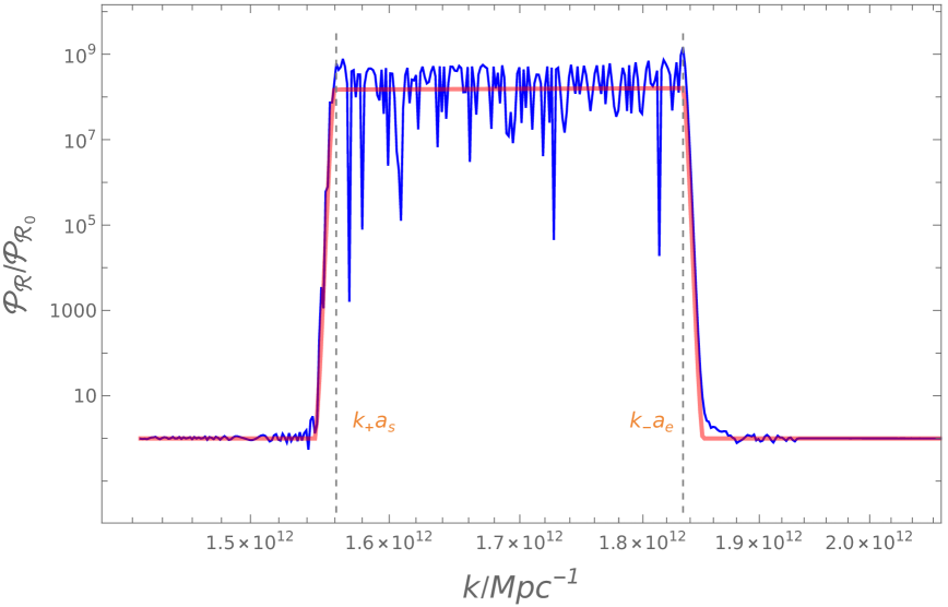
Figure 1: The normalized power spectrum enhancement $\mathcal{P}_{\mathcal{R}}/\mathcal{P}_{\mathcal{R}_{0}}$ versus $k/Mpc^{-1}$. Numerical solutions (blue) from $\mathcal{P}_{\mathcal{R}}/\mathcal{P}_{\mathcal{R}_{0}}=\frac{k^{3}}{2\pi^{2}}\left|\frac{u_{k}}{z}\right|^{2}/\mathcal{P}_{\mathcal{R}_{0}}$ demonstrate excellent agreement with analytical predictions (red) from Eq. (30), showing the characteristic plateau feature predicted by the resonant amplification mechanism.

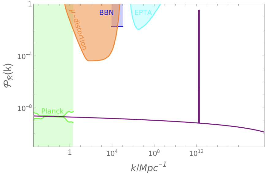
Figure 2: The primordial curvature perturbation power spectrum (solid purple line) with observational bounds. The spectrum satisfies constraints from CMB (green) Aghanim2020 , $\mu$ distortion (orange) D.J.Fixsen , BBN (blue) K.Inomata2016 , and EPTA observations (cyan) K.Inomata2019 , while achieving sufficient enhancement at small scales for PBH formation.

With parameters set to $m=9.0\times 10^{8}$, $w=1.3082\times 10^{5}$, $\Lambda=4.93\times 10^{-10}M_{\mathrm{pl}}^{10}$, $\phi_{s}=3.881M_{\mathrm{pl}}$, $\phi_{e}=3.871M_{\mathrm{pl}}$, $n=1\times 10^{7}M_{\mathrm{pl}}^{-1}$, and e-folding number $N\simeq 50$, our model predicts a tensor-to-scalar ratio $r\simeq 0.03$, which is in excellent agreement with current observations from Planck Aghanim2020 and the BICEP/Keck collaborations Ade2021 . Figure 1 illustrates the amplification of the curvature perturbation power spectrum in the resonant region $k_{+}a_{s}<k<k_{-}a_{e}$. The blue curve represents the numerical solution derived from $\mathcal{P}_{\mathcal{R}}/\mathcal{P}_{\mathcal{R}_{0}}=\frac{k^{3}}{2\pi^{2}}\left|\frac{u_{k}}{z}\right|^{2}/\mathcal{P}_{\mathcal{R}_{0}}$, while the red curve corresponds to the analytical approximation given by Eq. (30). As anticipated from the analysis in Eq. (28), this amplification produces a characteristic plateau in this region, indicating that the amplification factor is independent of the wavenumber $k$. The excellent agreement between numerical and analytical results validates the reliability of our theoretical framework and demonstrates that this mechanism can enhance the power spectrum by several orders of magnitude. Figure 2 presents the complete power spectrum of curvature perturbations obtained through numerical calculations of Eq. (11). This result highlights the significant enhancement achieved in the resonant region.

IV PBHs and SIGWs

During inflation, curvature perturbations are stretched beyond the Hubble horizon and later re-enter during the radiation- or matter-dominated eras. Sufficiently large perturbations induce significant density fluctuations, leading to gravitational collapse in high-density regions and forming PBHs. The PBH mass is related to the horizon mass at re-entry for a comoving wavenumber $k$

$$M(k)\simeq M_{\odot}\left(\frac{\gamma}{0.2}\right)\left(\frac{g_{*}}{10.75}\right)^{-\frac{1}{6}}\left(\frac{k}{1.9\times 10^{6}~\mathrm{Mpc}^{-1}}\right)^{-2},$$ (31)

where $\gamma\sim(1/\sqrt{3})^{3}$ is the ratio of PBH mass to horizon mass, $M_{\odot}$ is the solar mass, and $g_{*}=106.75$ represents the effective degrees of freedom during the early radiation-dominated era. The PBH formation rate is described by Young2014

$$\beta(M)=\frac{1}{2}\operatorname{erfc}\left(\frac{\delta_{c}}{\sqrt{2\sigma^{2}(M)}}\right),$$ (32)

where $\delta_{c}\simeq 0.4$ is the critical collapse threshold Musco2013 ; Harada2013 , erfc is the complementary error function, and $\sigma^{2}(M)$ is the variance of the coarse-grained density contrast, smoothing over the scale $k$, given by

$$\sigma^{2}(M(k))=\frac{16}{81}\int d\ln q\,W^{2}\left(qk^{-1}\right)\left(qk^{-1}\right)^{4}\mathcal{P}_{\mathcal{R}}(q).$$ (33)

Where $W$ represents the window function, which is chosen to be a gaussian function $W(x)=e^{-x^{2}/2}$ in this paper. The current fraction of PBHs in dark matter density is

$$\frac{\Omega_{\mathrm{PBH}}}{\Omega_{\mathrm{DM}}}=\int\frac{dM}{M}f(M),$$ (34)

where the PBH mass spectrum $f(M)$ is expressed as

$$f(M)\simeq\frac{\beta(M)}{1.84\times 10^{-8}}\left(\frac{\gamma}{0.2}\right)^{\frac{3}{2}}\left(\frac{10.75}{g_{*}}\right)^{\frac{1}{4}}\left(\frac{0.12}{\Omega_{\mathrm{DM}}h^{2}}\right)\left(\frac{M}{M_{\odot}}\right)^{-\frac{1}{2}}.$$ (35)

Based on the power spectrum Eq. (11) obtained in the previous chapter, our numerical results from Eq. (34) and Eq. (35) indicate that PBHs with a peak mass around $10^{-12}M_{\odot}$ could account for nearly all dark matter, with $\Omega_{\mathrm{PBH}}/\Omega_{\mathrm{DM}}\approx 0.997$. Figure 3 shows the mass spectrum of PBHs.

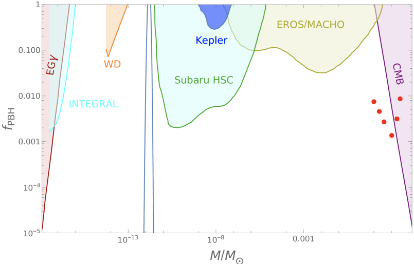
Figure 3: The PBH mass spectrum(solid light-blue line) and observational constraints, including data from EG$\gamma$ B.J.Carr2010 , WD P.W.Graham2015 , INTEGRAL R.Laha , Kepler K.Griest , Subaru HSC H.Niikura2019 , EROS/MACHO P.Tisserand , and CMB V. Poulin .

In parallel, SIGWs are generated during PBH formation through second-order tensor perturbations sourced by large curvature perturbations. The evolution of tensor perturbations $h_{ij}$ is governed by Baumann2007 ; Ananda2007

$$h_{ij}^{\prime\prime}+2\mathcal{H}h_{ij}^{\prime}-\nabla^{2}h_{ij}=-4\mathcal{T}_{ij}^{lm}S_{lm},$$ (36)

where $\mathcal{H}\equiv a^{\prime}/a$ is the conformal Hubble parameter, a prime represents differentiation with respect to conformal time, $\mathcal{T}_{ij}^{lm}$ is a projection operator, and $S_{ij}$ is the source term involving scalar perturbations $\Psi$

$$S_{ij}=4\Psi\partial_{i}\partial_{j}\Psi+2\partial_{i}\Psi\partial_{j}\Psi-\frac{1}{\mathcal{H}^{2}}\partial_{i}\left(\mathcal{H}\Psi+\Psi^{\prime}\right)\partial_{j}\left(\mathcal{H}\Psi+\Psi^{\prime}\right).$$ (37)

During the radiation-dominated era ($w=1/3$), the scalar perturbations $\Psi$ evolve as

$$\Psi_{k}(\eta)=\psi_{k}\frac{9}{(k\eta)^{2}}\left(\frac{\sin(k\eta/\sqrt{3})}{k\eta/\sqrt{3}}-\cos(k\eta/\sqrt{3})\right),$$ (38)

where $\psi_{k}$ is linked to the primordial curvature power spectrum $\mathcal{P}_{\mathcal{R}}(k)$. The gravitational wave energy density is computed as Kohri2018

$$\Omega_{\mathrm{GW}}\left(\eta_{c},k\right) =\frac{1}{12}\int_{0}^{\infty}dv\int_{|1-v|}^{|1+v|}du\left(\frac{4v^{2}-\left(1+v^{2}-u^{2}\right)^{2}}{4uv}\right)^{2}\mathcal{P}_{\mathcal{R}}(ku)\mathcal{P}_{\mathcal{R}}(kv)$$

$$\quad\times\left(\frac{3}{4u^{3}v^{3}}\right)^{2}\left(u^{2}+v^{2}-3\right)^{2}$$

$$\quad\times\left\{\left[-4uv+\left(u^{2}+v^{2}-3\right)\ln\left|\frac{3-(u+v)^{2}}{3-(u-v)^{2}}\right|\right]^{2}\right.$$

$$\quad\left.+\pi^{2}\left(u^{2}+v^{2}-3\right)^{2}\Theta(v+u-\sqrt{3})\right\},$$ (39)

where $\eta_{c}$ denotes the conformal time when SIGW production ceases. The present-day SIGW energy density spectrum is

$$\Omega_{\mathrm{GW},0}h^{2}=0.83\left(\frac{g_{*}}{10.75}\right)^{-1/3}\Omega_{\mathrm{r},0}h^{2}\Omega_{\mathrm{GW}}\left(\eta_{c},k\right),$$ (40)

where $\Omega_{\mathrm{r},0}h^{2}=4.2\times 10^{-5}$ is the current radiation density, and the frequency $f$ is related to $k$ as

$$f=1.546\times 10^{-15}\frac{k}{1\,\mathrm{Mpc}^{-1}}\,\mathrm{Hz}.$$ (41)

Through numerical calculations in (40) and utilizing (41) , we present the current SIGW energy spectrum in Figure 4. The frequency range of SIGW signals spans from $10^{-5}$ Hz to $5\times 10^{-2}$ Hz, corresponding to $\Omega_{\mathrm{GW},0}h^{2}$ values between $10^{-12}$ and $10^{-8}$. These signals fall within the sensitivity ranges of future gravitational wave detectors such as LISA, Taiji, and TianQin. This provides a promising avenue to probe PBHs and the early universe.

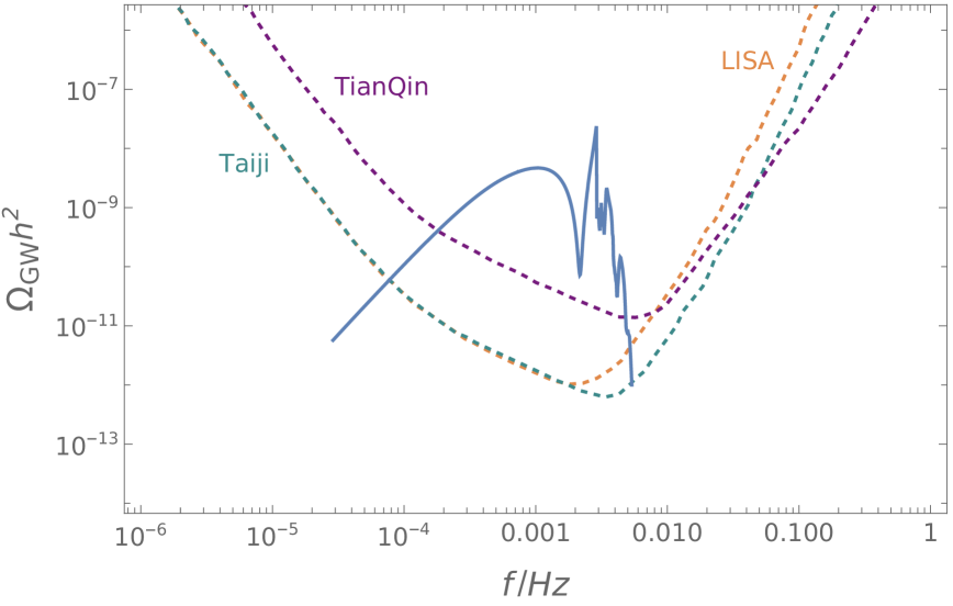
Figure 4: Present-day SIGW energy spectrum (solid blue line) compared with the sensitivity curves (dotted lines) of gravitational wave detectors TAIJI taiji , TIANQIN tianqin , and LISA lisa .

V conclusions

The formation of a large number of PBHs requires the power spectrum of curvature perturbations to reach an amplitude of at least $\mathcal{O}(10^{-2})$. Although observations of the CMB indicate that the power spectrum is nearly scale-invariant on large scales ($k\lesssim 1\,\mathrm{Mpc}^{-1}$), the amplitude of curvature perturbations on smaller scales ($k\gtrsim 1\,\mathrm{Mpc}^{-1}$) is not strictly constrained and may be significantly enhanced. In this study, we have proposed a new derivative coupling mechanism based on a non-minimal coupling inflation model. The coupling function consists of a constant term and a periodic term, where the constant term reduces the tensor-to-scalar ratio, and the periodic term amplifies curvature perturbations through sound speed resonance. The periodic coupling is designed to be short-lived and weak, ensuring negligible impact on the evolution of the background field. Our results show that the square of the sound speed undergoes periodic oscillations, transforming the curvature perturbation equation into a Mathieu equation on sub-horizon scales. The solution to this equation indicates that curvature perturbations can grow exponentially under certain conditions, confirming the effectiveness of the sound speed resonance mechanism in enhancing curvature perturbations. When these amplified curvature perturbations re-enter the Hubble radius during the radiation-dominated era, regions of sufficiently high density may undergo gravitational collapse, eventually forming PBHs. These PBHs could constitute an important component of dark matter. Furthermore, the formation of PBHs is accompanied by the generation of SIGWs, whose energy density spectrum, $\Omega_{\mathrm{GW},0}h^{2}$, exhibits distinct multi-peak features. It is shown from our results that these gravitational wave signals fall within the sensitivity ranges of next-generation detectors, such as Taiji, TianQin, and LISA, providing strong support for future observations and offering opportunities to test theoretical models.

- (1) B. Ya Zel dovich and I. D. Novikov, Soviet Astron.AJ (Engl. Transl.), 9, 602 (1967).
- (2) S. Hawking, Mon. Not. Roy. Astron. Soc. 152, 75 (1971).
- (3) B. J. Carr and S. W. Hawking, Mon. Not. Roy. Astron. Soc. 168, 399 (1974).
- (4) P. Meszaros, Astron. Astrophys. 37, 225 (1974).
- (5) B. J. Carr, Astrophys. J. 201, 1 (1975).
- (6) M. Y. Khlopov, B. A. Malomed, and Y. B. Zeldovich, Mon. Not. Roy. Astron. Soc. 215, 575 (1985).
- (7) O. Özsoy and G. Tasinato, Universe 9(5), 203(2023).
- (8) S. Bird, I. Cholis, J. B. Muñoz, Y. Ali-Haïmoud, M. Kamionkowski, E. D. Kovetz, A. Raccanelli, and A. G. Riess, Phys. Rev. Lett. 116, 201301 (2016).
- (9) S. Clesse and J. García-Bellido, Phys. Dark Univ. 15, 142 (2017).
- (10) M. Sasaki, T. Suyama, T. Tanaka, and S. Yokoyama, Phys. Rev. Lett. 117, 061101 (2016).
- (11) B. Carr, F. Kuhnel, and M. Sandstad, Phys. Rev. D 94, 083504 (2016).
- (12) P. Mróz, A. Udalski, J. Skowron, et al., Nature (London) 548, 183 (2017).
- (13) H. Niikura, M. Takada, S. Yokoyama, T. Sumi, and S. Masaki, Phys. Rev. D 99, 083503 (2019).
- (14) A. Katz, J. Kopp, S. Sibiryakov, and W. Xue, J. Cosmol. Astropart. Phys. 12, 005(2018).
- (15) A. Barnacka, J. F. Glicenstein, and R. Moderski, Phys. Rev. D 86, 043001 (2012).
- (16) P. W. Graham, S. Rajendran, and J. Varela, Phys. Rev. D 92, 063007 (2015).
- (17) H. Niikura, M. Takada, N. Yasuda, et al., Nat. Astron. 3, 524 (2019).
- (18) Y. F. Cai, X. Tong, D. G. Wang and S. F. Yan, Phys. Rev. Lett. 121, 081306 (2018).
- (19) Y. F. Cai, C. Chen, X. Tong, D. G. Wang and S. F. Yan, Phys. Rev. D 100, 043518 (2019).
- (20) N. Aghanim, Y. Akrami, M. Ashdown, et al. (Planck Collaboration), Astron. Astrophys. 641, A6 (2020).
- (21) J. Yokoyama, Phys. Rev. D 58, 083510 (1998).
- (22) S. Choudhury and A. Mazumdar, Phys. Lett. B 733, 270 (2014).
- (23) Y. Tada and S. Yokoyama, Phys. Rev. D 100, 023537 (2019).
- (24) S. S. Mishra and V. Sahni, J. Cosmol. Astropart. Phys. 04, 007(2020).
- (25) V. Atal, J. Cid, A. Escriva, and J. Garriga, J. Cosmol. Astropart. Phys. 05, 022(2020).
- (26) H. V. Ragavendra, P. Saha, L. Sriramkumar, and J. Silk, Phys. Rev. D 103, 083510 (2021).
- (27) N. Bhaumik and R. K. Jain, J. Cosmol. Astropart. Phys. 01, 037(2020).
- (28) H. Motohashi and W. Hu, Phys. Rev. D 96, 063503 (2017).
- (29) J. M. Ezquiaga, J. Garcia-Bellido, and E. Ruiz Morales, Phys. Lett. B 776, 345 (2018).
- (30) H. Di and Y. Gong, J. Cosmol. Astropart. Phys. 07, 007(2018).
- (31) G. Ballesteros and M. Taoso, Phys. Rev. D 97, 023501 (2018).
- (32) I. Dalianis, A. Kehagias, and G. Tringas, J. Cosmol. Astropart. Phys. 01, 037(2019).
- (33) T. J. Gao and Z. K. Guo, Phys. Rev. D 98, 063526 (2018).
- (34) M. Drees and Y. Xu, Eur. Phys. J. C 81, 182 (2021).
- (35) C. Fu, P. Wu, and H. Yu, Phys. Rev. D 102, 043527 (2020).
- (36) W. Xu, J. Liu, T. Gao, and Z. Guo, Phys. Rev. D 101, 023505 (2020).
- (37) J. Lin, Q. Gao, Y. Gong, Y. Lu, C. Zhang, and F. Zhang, Phys. Rev. D 101, 103515 (2020).
- (38) I. Dalianis and K. Kritos, Phys. Rev. D 103, 023505 (2021).
- (39) Z. Yi, Y. Gong, B. Wang, and Z. Zhu, Phys. Rev. D 103, 063535 (2021).
- (40) Q. Gao, Y. Gong, and Z. Yi, Nucl. Phys. B 969, 115480 (2021).
- (41) Z. Yi, Q. Gao, Y. Gong, and Z. Zhu, Phys. Rev. D 103, 063534 (2021).
- (42) T. Gao and X. Yang, Eur. Phys. J. C 81, 494 (2021).
- (43) M. Solbi and K. Karami, J. Cosmol. Astropart. Phys. 08, 056(2021).
- (44) Q. Gao, Sci. China Phys. Mech. Astron. 64, 280411 (2021).
- (45) M. Solbi and K. Karami, Eur. Phys. J. C 81, 884 (2021).
- (46) R. Cai, C. Chen, and C. Fu, Phys. Rev. D 104, 083537 (2021).
- (47) Q. Wang, Y. Liu, B. Su, and N. Li, Phys. Rev. D 104, 083546 (2021).
- (48) C. Germani and T. Prokopec, Phys. Dark Univ. 18, 6 (2017).
- (49) R. Zheng, J. Shi, and T. Qiu, Chin. Phys. C 46, 045103 (2022).
- (50) Z. Teimoori, K. Rezazadeh, M. A. Rasheed, and K. Karami, J. Cosmol. Astropart. Phys. 10, 018(2021).
- (51) C. Fu, P. Wu, and H. Yu, Phys. Rev. D 100, 063532 (2019).
- (52) C. Fu, P. Wu, and H. Yu, Phys. Rev. D 101, 023529 (2020).
- (53) I. Dalianis, S. Karydas, and E. Papantonopoulos, J. Cosmol. Astropart. Phys. 06 040(2020).
- (54) Z. Teimoori, K. Rezazadeh, and K. Karami, Astrophys. J. 915, 118 (2021).
- (55) S. Heydari, and K. Karami, Eur. Phys. J. C 82, 83 (2022).
- (56) S. Heydari, and K. Karami, J. Cosmol. Astropart. Phys. 03, 033(2022).
- (57) A. Karam, N. Koivunen, E. Tomberg, V. Vaskonen, and H. Veermae, J. Cosmol. Astropart. Phys. 03, 013(2023).
- (58) J. García-Bellido and E. R. Morales, Phys. Dark Univ. 18, 47 (2017).
- (59) S. Pi and J. Wang, J. Cosmol. Astropart. Phys. 06, 018(2023).
- (60) S. Choudhury, M. R. Gangopadhyay, and M. Sami, arXiv: 2301.10000.
- (61) D. Meng, C. Yuan, and Q. Huang, Sci. China Phys. Mech. Astron. 66, 280411 (2023).
- (62) B. Mu, G. Cheng, J. Liu, and Z. Guo, Phys. Rev. D 107, 043528 (2023).
- (63) R. Kawaguchi and S. Tsujikawa, Phys. Rev. D 107, 063508 (2023).
- (64) C. Fu and C. Chen, J. Cosmol. Astropart. Phys. 05, 005(2023).
- (65) L. Chen, H. Yu and P. Wu, Phys. Rev. D 106, 063537 (2022).
- (66) B. Gu, F. Shu, K. Yang and Y. Zhang, Phys. Rev. D 107, 023519 (2023).
- (67) Z. Yi, J. Cosmol. Astropart. Phys. 03, 048(2023).
- (68) S. Choudhury, S. Panda, M. Sami, arXiv: 2303.06066.
- (69) I. Dalianis, arXiv: 2310.11581.
- (70) J-X. Zhao, X-H. Liu, and N. Li Phys. Rev. D 107, 043515 (2023).
- (71) S. Choudhury, K. Dey, and A. Karde, arXiv: 2311.15065.
- (72) S. Heydari, K. Karami, arXiv: 2310.11030.
- (73) H. Firouzjahi, A. Talebian, arXiv: 2307.03164.
- (74) S. S. Mishra, E. J. Copeland, and A. M. Green, arXiv: 2303.17375.
- (75) K. Asadi, A. Nassiri-Rad, and H. Firouzjahi, arXiv: 2304.00577.
- (76) P. S. Cole, A. D. Gow, C. T. Byrnes, and S. P. Patil, J. Cosmol. Astropart. Phys. 08, 031(2023) .
- (77) S. Choudhury, S. Panda, and M. Sami, J. Cosmol. Astropart. Phys. 08, 078(2023).
- (78) D. Frolovsky, S. V. Ketov, Universe 9(6), 294(2023).
- (79) C. Chen, A. Ghoshal, Z. Lalak, Y. Luo, and A. Naskar, J. Cosmol. Astropart. Phys. 08, 041(2023).
- (80) B-Y. Su, N. Li, and L. Feng, arXiv: 2306.05364.
- (81) A. Cable, A. Wilkins, arXiv: 2306.09232.
- (82) A. Escrivà, V. Atal, and J. Garriga, J. Cosmol. Astropart. Phys. 10, 035(2023).
- (83) J. García-Bellido and E. Ruiz Morales, arXiv:1702.03901.
- (84) C. Germani and T. Prokopec, arXiv:1706.04226.
- (85) G. Ballesteros, J. B. Jiménez, and M. Pieroni, J. Cosmol. Astropart. Phys. 06, 016(2019).
- (86) A. Y. Kamenshchik, A. Tronconi, T. Vardanyan, and G. Venturi, Phys. Lett. B 791, 201 (2019).
- (87) M. A. Gorji, H. Mothhashi, and S. Mukohyama, J. Cosmol. Astropart. Phys. 02, 030(2022).
- (88) A. E. Romano, arXiv: 2006.07321.
- (89) G. Ballesteros, S. Céspedes, and L. Santoni, J. High Energy Phys. 2022(1), 74(2022).
- (90) R. Zhai, H. Yu, and P. Wu, Phys. Rev. D 106, 023517 (2022).
- (91) T. Qiu, W. Wang, and R. Zheng, Phys. Rev. D 107, 083018 (2023).
- (92) R. Zhai, H. Yu, and P. Wu, Phys. Rev. D 108, 043529 (2023).
- (93) C. Chen and Y. F. Cai, J. Cosmol. Astropart. Phys. 10, 068(2019).
- (94) C. Chen, X. H. Ma and Y. F. Cai, Phys. Rev. D 102 063526 (2020).
- (95) A. Addazi, S. Capozziello, and Q. Gan, J. Cosmol. Astropart. Phys. 08, 051(2022).
- (96) B. Li, C. Chen, and B. Wang, arXiv: 2307.03747.
- (97) Li-Yang Chen, Hongwei Yu, Puxun Wu, Phys. Lett. B 849, 138457(2024).
- (98) R. Cai, Z. Guo, J. Liu, L. Liu, and X. Yang, J. Cosmol. Astropart. Phys. 06, 013(2020).
- (99) T. Kobayashi, M. Yamaguchi, and J. Yokoyama, Prog. Theor. Phys. 126, 511 (2011).
- (100) S. Tsujikawa, Phys. Rev. D 85, 083518 (2012).
- (101) A. D. Felice and S.Tsujikawa, J. Cosmol. Astropart. Phys. 04, 029(2011).
- (102) A. D. Linde Phys Lett B 1983, 129: 177.
- (103) D. J. Fixsen, E. S. Cheng, J. M. Gales, J. C. Mather, R. A. Shafer, and E. L. Wright, Astrophys. J. 473, 576 (1996).
- (104) K. Inomata, M. Kawasaki, and Y. Tada, Phys. Rev. D 94, 043527 (2016).
- (105) K. Inomata and T. Nakama, Phys. Rev. D 99, 043511 (2019).
- (106) P. A. R. Ade, Z. Ahmed, M. Amiri, et al., Phys. Rev. Lett. 127, 151301 (2021).
- (107) B. J. Carr, K. Kohri, Y. Sendouda, and J. Yokoyama, Phys. Rev. D 81, 104019 (2010).
- (108) R. Laha, Phys. Rev. Lett. 123, 251101 (2019).
- (109) K. Griest, A. M. Cieplak, and M. J. Lehner, Phys. Rev. Lett. 111, 181302 (2013).
- (110) P. Tisserand, L. Le Guillou, C. Afonso, et al. (EROS-2 Collaboration), Astron. Astrophys. 469, 387 (2007).
- (111) V. Poulin, P. D. Serpico, F. Calore, S. Clesse and K. Kohri, Phys. Rev. D 96, 083524 (2017).
- (112) S. Young, C. T. Byrnes, and M. Sasaki, J. Cosmol. Astropart. Phys. 07, 045(2014).
- (113) T. Harada, C. M. Yoo, and K. Kohri, Phys. Rev. D 88, 084051 (2013).
- (114) I. Musco and J. C. Miller, Class. Quant. Grav. 30, 145009 (2013).
- (115) D. Baumann, P. J. Steinhardt, K. Takahashi and K. Ichiki, Phys. Rev. D 76, 084019 (2007).
- (116) K. N. Ananda, C. Clarkson, and D. Wands, Phys. Rev. D 75, 123518 (2007).
- (117) K. Kohri and T. Terada, Phys. Rev. D 97, 123532 (2018).
- (118) W. R. Hu and Y. L. Wu, Natl. Sci. Rev. 4, 685 (2017).
- (119) J. Luo, L. S. Chen, H. Z. Duan, et al. (TianQin), Class. Quant. Grav. 33, 035010 (2016).
- (120) P. Amaro-Seoane, H. Audley, S. Babak, et al. (LISA), arXiv:1702.00786.