Primer C-VAE: An interpretable deep learning primer design method to detect emerging virus variants

Abstract

Motivation:

Compared to Next Generation Sequencing (NGS), Polymerase Chain Reaction (PCR) is a more economical friendly and quicker method for detecting target organisms in laboratory and field settings, where primer design is a critical step. Especially in the context of epidemiology with rapidly mutating viruses, designing effective primers becomes increasingly challenging. Traditional primer design methods require substantial manual intervention and often struggle to ensure effective primer design across different strains within the same virus species. Similarly, for organisms with large and highly similar genomes, such as Escherichia coli and Shigella flexneri, designing primers to differentiate between these species is also critical but not easy. Therefore, more efficient primer design methods are necessary.

Results:

We employed a model based on a Variational Auto-Encoder (VAE) framework utilizing Convolutional Neural Networks (CNNs) as the primary method for identifying different variants. Subsequently, we extracted the convolutional layers from the VAE model for data post-processing to generate primers specific to different variants. Using SARS-CoV-2 as an example, our model effectively classified various variants (alpha, beta, gamma, delta, and omicron) with 98% accuracy on both the training and test sets, and successfully generated primers for each variant. The primers generated by our model appeared with a frequency exceeding 95% in their target variants and less than 5% in other variants. These primers demonstrated good performance in in-silico PCR tests. For the Alpha, Delta, and Omicron variants, our primer pairs produced fragments shorter than 200 bp in PCR tests, which can be utilized for designing further qPCR detection methods. Additionally, our model successfully generated effective primers for organisms with longer gene sequences, such as Escherichia coli and Shigella flexneri.

Conclusion:

Primer C-VAE is an interpretable deep learning based primer design approach to develop more specific primer pairs for target organisms. The method is a flexible, semi-automated and reliable primer design tool regardless of the completeness and the length of the gene sequence. The flexibility of the method allows users for further quantification applications, such as qPCR, and can be applied to a wide range of organisms, including those with large and highly similar genomes.

1 Introduction

Primer design plays a crucial role in modern molecular biology, providing a cost-effective and rapid approach through polymerase chain reaction (PCR) for organism detection in genetic testing and research. As Bustin and Huggett emphasize, ”primers are arguably the single most critical components of any PCR assay” [1]. The design of primers is fundamental to the entire PCR process, directly influencing the assay’s specificity and efficiency. However, with emerging virus variants such as Severe Acute Respiratory Syndrome Coronavirus 2 (SARS-CoV-2) that rapidly mutate, designing effective primers becomes increasingly challenging. The rapid mutation rates necessitate the development of new primer pairs to detect emerging variants, which significantly impacts treatment effectiveness and epidemiological studies. Similarly, for closely related bacteria like Escherichia coli (E. coli) and Shigella flexneri (S. flexneri) that share high genomic similarity, designing primers that differentiate between these species is essential for accurate detection. Therefore, developing efficient and reliable primer design methods is crucial for detection and effective treatment strategies.

Currently, High-throughput sequencing or Next Generation Sequencing (NGS) serves as the gold standard for identifying emerging virus variants, including SARS-CoV-2 variants [2]. However, NGS implementation requires sophisticated equipment and specialized expertise for both data generation and analysis. Sanger sequencing offers a less expensive alternative, but remains time-consuming for analyzing genome sequences of approximately 30 kb, such as SARS-CoV-2 [3]. This method requires fragmenting the entire sequence into multiple overlapping segments (approximately 700-900 bps each), sequencing each fragment individually, and reassembling these fragments through bioinformatic approaches. PCR assays provide a more economical and adaptable alternative to sequencing workflows for known gene detection, leading to their widespread adoption in both research and clinical applications [4, 5]. Conventional PCR assays require a target gene and a primer pair (forward and reverse) in standard PCR reagent mixture [6]. The successful execution of these assays depends critically on precisely designed PCR primers for specific target sequence binding.

1.1 Limitations of existing primer design methods

For reliable PCR testing, primer design is crucial and typically involves both forward and reverse primers. The process starts with gathering similar sequences containing the target region. Aligning these sequences allows for better visual examination and selection of conserved 18-25 base pair regions that include the target area. After identifying potential primers, their thermodynamic characteristics—including guanine-cytosine content (GC content), melting temperature, and possible secondary structures—must be assessed to ensure efficiency and reduce primer dimer formation. The complementary sequence to the antisense strand becomes the forward primer. A reverse primer must also be designed downstream following similar principles, but binds to the sense strand of the target DNA or RNA. For more details on this standard methodology, see [7].

In practice, however, the process is considerably more complex than theoretical descriptions suggest. Rather than simple sequence selection, it depends heavily on the designer’s expertise in sequence alignment, primer specificity assessment, and dimer prevention. For example, designing primers to detect the SARS-CoV-2 Alpha variant requires identifying a unique 18-25 nucleotide sequence within the 30,000-nucleotide viral genome that is specific to Alpha and meets strict thermodynamic parameters [8]. This demands extensive time comparing the sequence against other SARS-CoV-2 variants and related coronaviruses to ensure absolute specificity. These intricate requirements, combined with significant time investment and sustained concentration, make the process susceptible to human error and inconsistency.

While tools like Primer3 and Primer3Plus now exist for rapid generation of primers meeting basic requirements—reducing human error and decreasing time spent on repetitive tasks—these automatically generated primers cannot guarantee complete usability. Primer3 can quickly produce 30 primer pairs with suitable thermodynamic properties, yet many fail in actual PCR experiments. Additionally, these primers require further verification, as their specificity to target variants remains unconfirmed without supplementary testing.

A significant limitation of existing tools concerns input sequence length constraints. Primer3, for instance, only processes sequences up to 10,000 base pairs—making it unsuitable for viruses like SARS-CoV-2 with 30,000+ base pair genomes, and entirely inadequate for organisms like E. coli with over 5 million base pairs. Current systems simply cannot effectively handle such extensive genomic sequences.

Therefore, the limitations of existing primer design methods can therefore be summarized as:

1. Excessive dependence on specialist expertise and manual screening, resulting in time-intensive processes vulnerable to human error.

2. Inability to handle long genomic sequences, restricting applicability across diverse organisms.

3. Insufficient guarantees of primer specificity and effectiveness, requiring additional experimental validation.

To address these challenges, we propose a deep learning-based semi-automated primer design approach. This method overcomes many issues researchers currently face, eliminates gene length limitations, and provides more precise primer generation for organism variants. The result is a streamlined, more reliable primer design process particularly valuable for detecting emerging variants.

1.2 Proposed method

In this paper, we propose an interpretable deep learning approach for reliable primer design, developing both forward and reverse primers through a Variational Auto-Encoder (VAE) framework with Convolutional Neural Networks (CNNs). We introduce Primer C-VAE (Convolutional Variational Auto-Encoder for Primer design), a novel method that addresses critical limitations in existing primer design systems.

Our method handles multiple primer design scenarios, including: 1) designing primers for different variants within the same virus species, such as distinguishing between SARS-CoV-2 Alpha and Delta variants, and 2) designing primers for different organisms with similar large genomes, such as E. coli and S. flexneri. This approach specifically targets the shortcomings of conventional primer design methods to deliver more efficient and reliable results.

The methodology consists of two primary components: forward and reverse primer design. For forward primer design, we implement a preprocessing step to collect and validate gene sequences, ensuring data completeness and uniformity. Sequences that are incomplete or deviate from the mean length by more than 1/3 or are shorter than 2/3 are excluded. We then employ a C-VAE framework to effectively distinguish target gene sequences from others—whether different variants of the same virus or sequences from different organisms. The convolutional filters in our C-VAE encoder extract flexible-length sequences (18-25 base-pairs) as candidate primer features. These candidates undergo evaluation against thermodynamic criteria and dimer checks to identify viable forward primers.

The reverse primer design follows a similar approach with one key difference: we use the identified forward primers to locate downstream sequences of the target. These downstream sequences, along with a synthetically generated dataset matching their nucleotide distribution, serve as inputs to our C-VAE model. Following the same evaluation process as for forward primers, we generate reverse primers that pair with the forward primers to create complete primer sets. We validate these primer pairs using Primer-BLAST [9] to minimize off-target amplifications and prevent primer annealing to both human genome sequences and similar microbial genomes. Finally, in-silico PCR [8] verifies their specificity and effectiveness in detecting variants of interest or target organisms.

Our method introduces the first VAE framework-based deep learning approach for flexible-length primer design, encompassing both forward and reverse primers. It demonstrates remarkable effectiveness in designing exclusive primers for sequence sub-classification tasks, such as differentiating SARS-CoV-2 virus variants, and for distinguishing between organisms with large and highly similar genomes, including E. coli (4.5-5.5 Mb) and S. flexneri (4.2-4.7 Mb).

This deep learning-based semi-automated primer design process delivers several critical advancements. First, it precisely generates complete primer pairs for PCR assays capable of detecting specific virus variants—a capability previously unavailable. Second, it eliminates restrictions on input genome sequence length for primer design. Additionally, the method maintains effectiveness even with incomplete genome sequences, providing practical utility in real-world applications.

Performance metrics confirm the method’s exceptional reliability. For SARS-CoV-2 variant classification, our approach achieves over 98% accuracy, with generated primer pairs exhibiting high specificity: present in over 95% of target variant sequences while occurring in less than 5% of other variants (with Omicron as the sole exception at 80% and 20% respectively). Similarly, for E. coli and S. flexneri classification, the method achieves over 96% accuracy, with primers showing equivalent specificity—present in over 95% of target organism sequences and under 5% in non-target organisms.

A significant advantage of our approach is that primer pairs designed for SARS-CoV-2 variants generate amplicons under 200 base pairs in length. This characteristic enables versatile application across various PCR techniques, including conventional PCR, RT-PCR, and qPCR assays targeting specific variants. Through these innovations, our method effectively addresses the limitations of existing primer design approaches while delivering substantially improved efficiency and reliability throughout the primer design process.

1.3 Related work

Recent advances in computational biology have led to the development of diverse methodologies for efficient primer design in molecular diagnostics. Primer3, introduced in 2000, remains one of the most widely utilized open-source applications for this purpose [10, 11]. This software implements established thermodynamic models to calculate oligonucleotide melting temperatures during target hybridization and predict secondary structure stability. Despite its effectiveness for species-level detection of viral and bacterial targets, Primer3 generates numerous suboptimal primers and demonstrates limited capability in differentiating between variants of the same viral species, such as SARS-CoV-2 lineages. Additionally, its maximum input sequence constraint of 10,000 base pairs proves insufficient for organisms with extended genomes, particularly bacterial pathogens like E. coli with genome sizes of 4.5-5.5 Mb.

Researchers have developed several alternative approaches to address these limitations. One notable strategy employs finite state machines (FSMs) to classify PCR primers into suitable and unsuitable categories [12]. This approach effectively complements Primer3 by facilitating optimal primer selection from its output. However, the methodology requires comprehensive primer datasets for training, limiting its applicability for rapidly evolving pathogens such as SARS-CoV-2, where frequent retraining becomes necessary.

Genetic algorithm-based approaches offer another solution for primer design challenges [13]. These methods overcome sequence length restrictions and potentially provide enhanced precision compared to Primer3. Nevertheless, they present several limitations: their dependence on random mutation simulations reduces stability for viruses with multiple mutation sites and rapid evolution rates; they necessitate species-specific parameter optimization for crossover probability (pc), mutation probability (pm), and population size (p); and like many optimization techniques, they risk convergence to local optima rather than global solutions. Furthermore, while these methods excel at species-level primer design, they lack capabilities for variant-specific detection.

Recent evolutionary algorithm developments have produced methods specifically targeting SARS-CoV-2 variant detection through comprehensive forward and reverse primer design [14]. However, these approaches heavily rely on identification of significant mutation regions to guide primer discovery. This dependency creates inherent instabilities when mutation patterns shift and limits generalizability to other viral pathogens due to reliance on fixed mutation sites. Moreover, these methods fail in scenarios where mutation information remains unavailable, rendering primer design impossible under such circumstances.

Machine learning approaches, such as those developed in [15], address SARS-CoV-2 forward primer design with several advantages, including unrestricted sequence length input and automated primer generation capabilities. Unlike genetic and evolutionary algorithms, these methods function independently of known mutations or species-specific parameter optimization, resulting in enhanced stability and computational efficiency. Despite these advances, significant limitations persist: current implementations generate only forward primers of fixed length (21 base pairs), require manual reverse primer selection based on researcher expertise, and lack capability to distinguish between viral variants, operating exclusively at the species level.

Our methodology presents multiple significant advantages over conventional primer design approaches and previously described techniques. Most notably, it substantially reduces manual intervention required to identify signature genomic regions within datasets containing thousands of sequences. Building upon the framework established in [15], our approach maintains compatibility with sequences of unlimited length, efficiently processing both the approximately 30,000-nucleotide SARS-CoV-2 genome and bacterial genomes exceeding 5 Mb, such as those of E. coli strains. Quantitative comparative analysis demonstrates markedly enhanced efficiency in primer design for sequence sub-classification compared to Primer3, as documented in Table 16. A fundamental innovation in our method is the development of a VAE-based deep learning architecture specifically optimized for reverse primer design, incorporating three complementary feature extraction paradigms. The system generates primers of variable length (18-25 base pairs) requiring only the target organism’s genomic sequences as input, thereby eliminating preprocessing requirements for researchers investigating rapidly evolving pathogens or microorganisms with extensive genomes. Furthermore, given the demonstrated sequence classification accuracy of our approach, this computational framework exhibits considerable potential for primer design across diverse viral and bacterial species, offering particular utility in scenarios where mutation information remains inaccessible or incomplete.

1.4 Outline of the paper

The remainder of this paper is organized as follows. Section 2 presents a comprehensive description of our Primer C-VAE methodology, detailing the four sequential computational stages for primer design. We begin with genomic data acquisition and bioinformatic preprocessing to establish sequence alignment matrices suitable for neural network input. We then describe our convolutional variational autoencoder architecture for forward primer candidate generation, followed by our novel approach to reverse primer design, and conclude with rigorous validation procedures incorporating both BLAST sequence similarity analysis and in-silico PCR amplification simulation.

Section 3 presents the experimental validation of our methodology through two distinct applications. First, in Section 3.1, we demonstrate the effectiveness of Primer C-VAE in designing variant-specific primers for SARS-CoV-2, achieving exceptional discriminative capacity between Alpha, Beta, Gamma, Delta, and Omicron variants. Second, in Section 3.2, we extend our validation to organisms with substantially larger genomes, successfully developing primers that can discriminate between the closely related bacterial species Escherichia coli and Shigella flexneri.

Section 4 provides a comprehensive discussion of our findings, comparing our deep learning-assisted approach with traditional primer design methodologies, analyzing the advantages and limitations of our framework, and exploring potential future enhancements. We conclude by highlighting the significant contribution of Primer C-VAE as a novel computational paradigm for designing primers targeting specific organism detection, particularly for organisms with substantial genomic heterogeneity across variants.

The appendices provide supplementary materials including detailed descriptions of data collection and preprocessing protocols, feature extraction and evaluation metrics, flowcharts illustrating our methodology, BLAST and in-silico PCR validation results, and comparative analyses with existing primer design tools.

2 Process primer design with Primer C-VAE

Our Primer C-VAE methodology encompasses four sequential computational stages for integrated primer design (Figure 1). Stage I focuses on genomic data acquisition and bioinformatic preprocessing to establish sequence alignment matrices which suitable for neural network input. Stage II implements forward primer candidate generation through our convolutional variational autoencoder architecture, extracting discriminative genomic signatures from the preprocessed sequence data. Stage III executes the reverse primer design protocol, employing the forward primer candidates identified in Stage II as reference points to derive complementary reverse primers with optimal thermodynamic properties. Stage IV consists of rigorous validation procedures, incorporating both BLAST sequence similarity analysis and in-silico PCR amplification simulation to confirm primer specificity and amplification efficiency.

Figure 1: Pipeline for Primer Design

The Primer C-VAE methodology comprises four interconnected computational stages. Stage I (Data Acquisition and Pre-processing) encompasses sequence acquisition from genomic repositories, systematic taxonomic annotation, and strategic data curation to establish high-quality training datasets for downstream analysis. Stage II (Forward Primer Design) implements our trained convolutional variational autoencoder architecture to generate initial primer candidates, followed by frequency distribution analysis and thermodynamic property assessment to identify optimal forward primers with maximal discriminative capacity. Stage III (Reverse Primer Design) analyzes the downstream genomic regions adjacent to selected forward primer binding sites across target organism sequences, applying the C-VAE model in a second iteration to generate complementary reverse primer candidates, which undergo similar frequency and thermodynamic suitability filtering protocols. Stage IV (In-silico PCR and Primer-BLAST Validation) integrates selected forward and reverse primers into functional amplification pairs, evaluates their combinatorial properties including amplicon size and primer-dimer potential, and validates specificity through hierarchical assessment via BLAST sequence alignment followed by in-silico PCR amplification simulation.

The subsequent sections present a comprehensive examination of our computational methodology, commencing with genomic data acquisition pipelines and bioinformatic preprocessing algorithms. We subsequently elucidate the primer design framework, detailing the neural network-based feature extraction mechanisms and quantitative evaluation metrics implemented for both forward and reverse primer candidate selection. The discussion concludes with a comprehensive analysis of primer pair validation procedures.

2.1 Stage I: Data Acquisition and Pre-processing

Data acquisition.

The genomic sequence data utilized in this investigation was sourced from two authoritative repositories: GISAID (Global Initiative on Sharing Avian Influenza Data, [16]) and NCBI (National Centre for Biotechnology Information, [17]). These repositories provided SARS-CoV-2 variant sequences, Escherichia coli and Shigella flexneri genomic sequence data. The acquired sequences served multiple computational objectives: training the Convolutional Variational Auto-Encoder (C-VAE) model for target organism classification, generating candidate primers through the trained neural network, identifying downstream regions for reverse primer design, and conducting specificity verification through comparative sequence analysis. Our comprehensive dataset comprises 8,939 E. coli and 5,373 S. flexneri gene sequences from NCBI, supplemented with 473,645 SARS-CoV-2 sequences from GISAID representing five distinct variants (Alpha, Beta, Gamma, Delta, and Omicron), classified according to World Health Organization (WHO) nomenclature, Pango lineage classification system, and GISAID clade designation. Detailed sample distributions with corresponding taxonomic labels are presented in Appendix Table 6.

Data pre-processing.

Our pre-processing protocol implements adaptive sequence length filtration based on organism-specific genomic characteristics. For most organisms, we compute mean sequence lengths and eliminate sequences deviating more than 1/3 above or below this central value to ensure dataset uniformity for effective primer design. However, for viruses with relatively compact and complete genomic sequences, such as SARS-CoV-2, we modify this criterion by removing only sequences shorter than 2/3 of the mean length, thereby preserving dataset integrity. Following filtration, we determine the maximum sequence length ($max\_vector$) within each dataset and standardize all genome sequences through strategic ’N’ nucleotide padding, generating uniform $1\times 1\times max\_vector$ dimensional matrices. In our SARS-CoV-2 dataset, sequences averaged 29-30 kilobases with a maximum length of 31,079 base pairs, and filtering removed only sequences shorter than 20 kilobases, resulting in standardized $1\times 1\times 31,079$ matrices for neural network input. Variant-specific average sequence lengths are documented in Appendix Table 7.

Unlike Large Language Models (LLMs) capable of processing natural language or direct DNA/RNA sequences, our neural architecture requires numerical representation of categorical genomic data (nucleotides ’A’, ’T’, ’C’, or ’G’) [18]. While traditional bioinformatic approaches employ either One-Hot or K-mer encoding strategies, we primarily implement Ordinal Encoding as our default nucleotide representation method, as defined in Equation 1. This computational approach offers superior efficiency and implementation simplicity for convolutional neural networks compared to One-Hot Encoding, while providing enhanced flexibility relative to K-mer Encoding while maintaining comparable performance metrics [19]. We also provide One-Hot Encoding as an alternative representation strategy when appropriate.

Prior to neural network input, each standardized sequence undergoes Ordinal Encoding according to the function defined in Equation 1, with the resulting transformation illustrated in Appendix Figure 14.

$$Y:=f(x):=\left\{\begin{aligned} 0&\quad\mbox{ if }&x=N,\\ 1&\quad\mbox{ if }&x=C,\\ 2&\quad\mbox{ if }&x=T,\\ 3&\quad\mbox{ if }&x=G,\\ 4&\quad\mbox{ if }&x=A.\\ \end{aligned}\right.$$ (1)

To facilitate downstream analysis and biological interpretation, we implement an inverse transformation function that converts numerical outputs back to standard nucleotide representations. For organism classification objectives, taxonomic label data undergoes One-Hot encoding; for example, SARS-CoV-2 variant classification involving five distinct variants utilizes a $1\times 5$ dimensional vector representation.

Data selection.

Following pre-processing, we implemented a structured data partitioning strategy addressing three distinct computational requirements: model training, validation, and testing. Additionally, during the primer design phase, target organism sequences were systematically selected to generate candidate primers. These candidates subsequently required multiple reference sequence sets for comprehensive specificity evaluation, including: assessment of primer specificity to the target organism, calculation of appearance frequencies to minimize off-target amplification potential, and verification of non-complementarity to both human genomic sequences and related microbial genomes to prevent cross-reactivity. Our data selection protocol comprised three principal stages: 1) partitioning for neural network training, validation, and performance testing; 2) sequence selection for primer candidate generation; and 3) reference dataset compilation for primer specificity evaluation. A detailed methodological example of our data selection procedure for SARS-CoV-2 variant-specific primer design is presented in Table 1 for reference.

2.2 Stage II: Forward Primer Design

Primer C-VAE architecture.

We utilize a dataset of pre-processed genome sequences standardized into input-format matrices, $\mathcal{D}=\{seq_{1},seq_{2},\cdots,seq_{n}\}$, where each $seq_{i}$ represents a $1\times 1\times max\_vector$ genome sequence matrix. Our C-VAE model classifies these sequences into target and non-target classes. For variant-specific primer design, we classify organisms into distinct categories—for example, SARS-CoV-2 variants are classified as Alpha, Beta, Gamma, Delta, or Omicron. The C-VAE learns latent space representations of input sequences, which we then use to generate decoder outputs and classification labels. Figure 2 illustrates this model architecture.

Figure 2: Primer C-VAE architecture

Note: Primer C-VAE architecture implements a specialized convolutional encoder framework for discriminating genomic features between target organisms and their variant populations. This deep learning system integrates three critical functional modules: (1) a multi-layer convolutional encoder that systematically extracts hierarchical sequence features from raw genomic data, (2) a variational representation space where latent vectors $z$ are stochastically sampled via the reparameterization technique utilizing the learned distributional parameters $\mu$ and $\log\sigma^{2}$, and (3) a bifurcated computational pathway featuring both a classifier component for precise sequence categorization and a reconstruction decoder for generating sequence outputs. The architecture’s training protocol optimizes these components simultaneously to maximize feature discrimination while preserving biological sequence integrity.

The C-VAE model incorporates a five-layer encoder architecture: dual convolutional layers (Conv2D) with ReLU activation functions, paired max-pooling layers (MaxPool2D), and a terminal fully connected layer (FC) integrating both ReLU activation and batch normalization (BN). The hierarchical convolutional filtration system progressively extracts sequence features, with the initial layer isolating biologically significant motifs and subsequent layers identifying complex structural patterns. ReLU transformation significantly enhances computational efficiency and gradient propagation during backpropagation [20]. The strategically positioned max-pooling operations reduce spatial dimensionality while preserving critical feature information, enabling the fully connected layer to effectively integrate these multi-level features for downstream analysis.

Within the model’s variational framework, the latent representation $z$ is derived through statistical reparameterization, utilizing a specialized sampling function parameterized by encoder-generated $\mu$ and $\log\sigma^{2}$ vectors. The architecture bifurcates into complementary processing pathways: a classification branch that leverages the latent embeddings for sequence categorization, and a reconstruction branch where the decoder—implementing an inverted encoder topology—regenerates the input sequences from their compressed latent representations.

The decoder component serves dual analytical functions: precise sequence reconstruction and differential genomic region identification. This comparative reconstruction methodology facilitates detection of high-variability genomic loci between organism variants. Although these identified regions may not directly contribute to classification performance, they provide essential biological insights for primer design by highlighting genomic segments exhibiting elevated mutation frequencies. This integrated dual-objective approach ensures preservation of sequence-specific signatures while offering an interpretable analytical framework for identifying variant-discriminative regions with biological significance.

2.2.1 Model Training

During the pre-processing phase, input genomic sequences undergo standardization to achieve uniform dimensionality, utilizing the maximum sequence length as the standardization reference point. Each sequence is transformed into a structured $1\times 1\times max\_vector$ tensor representation for optimal compatibility with the C-VAE architecture. Following comprehensive data curation, the C-VAE model undergoes training on the prepared dataset to extract discriminative genomic signatures that differentiate target organisms from non-target variants. The training process implements the Adam optimization algorithm [21] with adaptive learning rate parameters, combined with a binary cross-entropy classification objective ($\mathcal{L}_{class}$). This classification loss is computationally executed through PyTorch’s Binary Cross Entropy with Logits function, facilitating numerical stability during gradient-based optimization [22].

The training methodology incorporates multiple objective components within its optimization framework. The reconstruction loss ($\mathcal{L}_{recon}$), quantified as the Mean Squared Error between input sequences and their corresponding reconstructions, ensures preservation of essential genomic characteristics in the model’s latent representation. Concurrently, the Kullback-Leibler divergence loss ($\mathcal{L}_{KL}$)functions as a regularization mechanism that constrains the latent space distribution toward a standard normal distribution, mathematically formulated as:

$$\mathcal{L}_{KL}=-0.5\sum(1+\log\sigma^{2}-\mu^{2}-\sigma^{2})$$

The comprehensive loss function integrates multiple training objectives to optimize the classification-enhanced Variational Autoencoder framework:

$$\mathcal{L}_{total}=\mathcal{L}_{recon}+\beta\ \cdot\mathcal{L}_{KL}+\lambda_{class}\cdot\mathcal{L}_{class}+\lambda_{reg}\cdot\mathcal{L}_{reg}$$

In this formulation, $\mathcal{L}_{reg}$ represents the L2 regularization term that mitigates overfitting by constraining parameter magnitudes. The hyperparameters $\beta$, $\lambda_{class}$, and $\lambda_{reg}$ cserve as balancing coefficients that modulate the relative contributions of each objective component during optimization. While the primary optimization focus centers on minimizing $\mathcal{L}_{class}$ to enhance classification performance, the integrated loss function ($\mathcal{L}_{total}$) ensures comprehensive sequence representation learning. This multi-objective optimization strategy proves particularly advantageous for specialized genomic applications such as primer design for virus variant detection, where both accurate classification and identification of mutation-prone genomic regions are of critical biological significance.

2.2.2 Feature Extraction and Forward Primer Generation

Following successful training of the C-VAE model, we implement a systematic approach for candidate forward primer extraction through four computationally distinct feature identification methodologies. Of these specialized techniques, three leverage the discriminative capabilities of the convolutional encoder architecture, while the fourth utilizes the sequence reconstruction properties of the decoder component.

The encoder’s initial convolutional layer, specifically optimized to capture biologically significant nucleotide motifs and sequence patterns, consists of 12 specialized filters with a $1\times N$ dimensional kernel configuration, where $N$ precisely corresponds to the target length of the generated primer sequences. Three distinct algorithmic approaches extract variable-length genomic fragments (ranging from 18-25 nucleotides) as candidate primer regions by applying specialized post-processing operations to the feature activation maps generated by the first convolutional layer: 1) Pooling method, 2) Top method, and 3) Mix method. The fourth complementary approach, 4) Reconstruction method, operates through fundamentally different mechanisms by analyzing differential patterns within the decoder-generated sequence representations.

Pooling method.

This approach adapts classical max-pooling principles while implementing a critical methodological distinction: rather than merely extracting maximum values, it systematically identifies and preserves positional information of activation maxima within each defined pooling region. The computational implementation involves applying custom maximum-pooling operations to individual filter activation maps, as visualized in Fig. 3. The precise nucleotide positions corresponding to maximum activation values are recorded in a dedicated Position file, with this computational process executed independently across all 12 filter channels to ensure comprehensive feature capture.

Figure 3: Feature extraction from the filter files by simulating maximum pooling operation.

Top method.

Unlike the spatially-constrained pooling approach, this global selection methodology operates without defined pooling regions, instead utilizing a parametrized ”top variable” to identify activation maxima across the entire feature space. This algorithm systematically records a predetermined number of maximum activation positions equal to the specified top variable parameter. Consequently, the identification of significant nucleotide positions directly correlates with the selected top variable value. To establish optimal parameterization, we conducted comprehensive performance analyses using various percentages of the total nucleotide count in the target gene sequence: 75 (0.25%), 125 (0.5%), 175 (0.58%), and 250 (0.83%) positions in Alpha and Delta variants for the SARS-CoV-2 primer design investigation. The comparative results, fully documented in Appendix Table 9, demonstrate that 175 positions (0.58%) represents the optimal parameter configuration, providing efficient computational performance while maximizing primer generation effectiveness and maintaining superior occurrence frequency of generated primers within target variant sequences.

Mix method.

This hybrid approach integrates elements from both the pooling and top methods, requiring both a pooling window size and a top variable. The process involves executing the pooling operation initially, followed by identifying and recording the positions of top maximum values within each pooling region. Based on empirical testing of the previous methods, we established that optimal performance is achieved using a maximum pooling window size of $1\times 500$ while recording and preserving the top 10 positions of maximum data within each pooling region.

Reconstruction method.

This method utilizes the decoder-generated reconstructed sequence to extract candidate primers. While the reconstructed sequence maintains the same length as the input sequence, it exhibits nucleotide variations at specific positions. This divergence is not a limitation but rather a design feature: the decoder, while trained to reconstruct the input sequence, identifies regions where nucleotide conservation is less critical for discriminating between target and off-target organisms. Conserved regions in the reconstructed sequence likely represent robust, functionally consistent segments, whereas divergent regions potentially indicate either discriminative sequence features between target and non-target organisms or genomic loci exhibiting elevated mutation frequencies among variant populations. The method systematically identifies and records positions exhibiting the highest degree of nucleotide divergence from the input sequence. The complete reconstruction process is illustrated in Fig. 4.

Figure 4: Feature extraction from the reconstructed sequence by identifying nucleotide divergence.

Our novel primer design methodology begins by identifying key nucleotide positions through computational feature extraction. These strategic positions serve as central anchoring points for potential primers. We construct complete primers by systematically incorporating flanking sequences while maintaining customizable lengths ranging from 18 to 25 base pairs, according to user specifications.

The design process integrates positional data with input genetic sequences to identify variant-specific features. Specifically, we utilize maximum value positions recorded in Position files to locate corresponding nucleotides within the input sequence. From each identified central nucleotide, we extend symmetrically in both directions to achieve the target primer length. For instance, a 25-base pair primer comprises the central nucleotide plus 12 nucleotides upstream and 12 nucleotides downstream. This approach ensures the incorporation of discriminatory features essential for accurate variant classification, as these central positions correspond to significant elements identified in the convolutional neural network layer.

We subject each candidate primer to rigorous quality assessment, evaluating thermodynamic properties, potential for dimer formation, and frequency of occurrence within target organism sequences. This comprehensive evaluation minimizes off-target amplification risk and maximizes specificity. As illustrated in Figure 5, our systematic approach to primer generation and validation ensures all candidates meet established design criteria [24, 25] before classification as viable forward primers. These essential criteria encompass:

Figure 5: Computational workflow for feature extraction and forward primer design. The pipeline initiates with raw sequence data processing through a neural encoder framework. We implement four distinct feature extraction algorithms to identify significant nucleotide positions. These positional data are systematically documented in position files that guide subsequent primer generation. Candidate primers undergo comprehensive validation against thermodynamic and specificity criteria before final classification as optimized forward primers.

1. Length of 18-25 nucleotides;

2. 40-60 % GC content;

3. Start and end with 1-2 G/C pairs;

4. Melting temperature (Tm) of 50-60^∘C (using on Primer3; also see [26]);

5. Primer pairs should have a Tm difference within 5^∘C;

6. Primer pairs should not have self-complementary regions of more than 5 pairs (based on IDT oligo-analyzer [27]).

Our validation process implements a comprehensive assessment of primer specificity through rigorous appearance rate analysis. We require candidate forward primers to exhibit unique occurrence patterns within target organism genomes to effectively minimize off-target amplification. Both absence of binding sites and multiple sequence matches can trigger mis-priming events, potentially leading to PCR failure [28].

For applications targeting variant-specific detection, we establish dual-threshold specificity criteria: primers must demonstrate ¿95% occurrence frequency within their corresponding variant genome sequences while maintaining minimal cross-reactivity (¡5%, optimally 0%) with non-target variants or related species. This stringent dual-parameter approach ensures exceptional detection sensitivity for intended targets while simultaneously providing robust discrimination against closely related genetic sequences.

2.3 Stage III: Reverse Primer Design

Traditional primer design methodology establishes that reverse primers must be positioned downstream from forward primers. The distance between these primers directly determines the amplicon length. For example, to generate a 200 base pair amplicon, researchers position the reverse primer binding site exactly 200 base pairs downstream from the forward primer.

Building upon these established principles, we have developed a novel deep learning approach specifically for reverse primer design. Our method introduces significant improvements over conventional techniques. Unlike the forward primer design process, our reverse primer algorithm requires different preprocessing steps. It operates exclusively on two input types: 1) validated forward primers and 2) their corresponding target organism gene sequences. This targeted focus enables more efficient primer selection through computational analysis of pre-qualified sequence regions.

2.3.1 Data pre-processing for generating the downstream dataset

The reverse primer design process requires two specific inputs: target variant sequences and validated forward primers. Our preprocessing workflow begins by precisely locating validated forward primers within target sequences, followed by systematic analysis of potential reverse primer binding regions. These binding regions extend from the forward primer position to the sequence’s 3’ terminus. Since DNA sequences are conventionally oriented in the 5’ to 3’ direction, reverse primer binding sites must be positioned downstream of the forward primer.

We segment each variant genome sequence containing validated forward primers into three distinct functional regions (illustrated in Fig. 7):

1. Upstream region: extending from the 5’ terminus to the nucleotide preceding the forward primer;

2. Forward primer region: encompassing the complete forward primer sequence;

3. Downstream region: spanning from the forward primer’s terminal nucleotide to the 3’ terminus.

For reverse primer design, we isolate and preserve only the downstream region, creating a specialized downstream dataset. This targeted approach confines the search space to biologically relevant regions while significantly reducing computational complexity.

Figure 6: Functional segmentation of target gene sequences for reverse primer design. The division creates three distinct regions: upstream, forward primer, and downstream regions. Note that the position and length of each downstream region varies uniquely depending on the binding location of its corresponding validated forward primer within the sequence.

Figure 7: The downstream sequences analysis of target genome sequences.

2.3.2 Generation of Synthetic Downstream Data

The C-VAE model previously employed for forward primer design has been adapted for reverse primer design. However, this adaptation introduces a significant methodological challenge: the input data structure now exclusively comprises downstream regions relative to validated forward primer binding sites (illustrated in Fig. 7) from a single variant. This single-variant approach results in a problematic single-label classification task that lacks comparative information necessary for effective feature discrimination. Without sufficient contrasting data, the model risks suboptimal feature extraction, where any solution satisfying the loss function might be erroneously accepted as optimal.

To overcome this inherent limitation, we developed a synthetic reference dataset that transforms the task into a meaningful binary classification problem. This synthetic dataset is generated through rigorous statistical analysis of nucleotide compositions present in authentic downstream sequences. Specifically, we calculate the precise ATCG content distribution patterns of original sequences, then generate random sequences that faithfully maintain these statistical properties to serve as the second classification label during model training. For implementation clarity, consider our application to the Delta variant of SARS-CoV-2 with the validated forward primer ’CTACCGCAATGGCTTGTCTTG’. Our procedure follows four sequential steps: 1) isolation of Delta variant genome sequences; 2) extraction of downstream regions identified during pre-processing; 3) analysis of nucleotide distribution patterns (shown in Fig. 7); and 4) generation of a synthetic downstream dataset that preserves these distributional characteristics. This refined methodology ensures the model receives sufficiently contrasting information to enable effective feature learning during the reverse primer design process.

2.3.3 Model Training and Feature Extraction

The C-VAE model architecture and associated loss functions employed for reverse primer design remain architecturally identical to those utilized in our forward primer design methodology. However, we now apply this framework specifically to the synthetic downstream dataset. Our training objective focuses explicitly on discriminating between authentic biological downstream sequences and their computationally generated synthetic counterparts. This binary classification paradigm enables the model to capture biologically significant sequence patterns that might otherwise remain undetected in a single-class approach.

Through this contrastive learning framework, the model develops sophisticated feature extraction capabilities tailored specifically for reverse primer design applications. Despite the synthetic sequences maintaining statistically similar nucleotide distributions to authentic sequences, they lack the evolutionary constraints and functional patterns inherent in genuine biological sequences. By learning to identify these subtle distinguishing characteristics, the model extracts features that reflect genuine biological constraints rather than merely statistical properties of nucleotide distribution. This biologically-informed feature extraction process significantly enhances the subsequent reverse primer design phase by prioritizing sequence patterns with functional relevance.

2.4 Stage IV: In-silico PCR and Primer-BLAST Validation

FFollowing the reverse primer design phase, all candidate primer pairs undergo comprehensive in-silico validation through standardized virtual PCR simulation protocols [8]. This computational approach enables systematic assessment of theoretical PCR amplification efficiency and primer-target specificity prior to laboratory implementation. Our reverse primer design process methodologically parallels the forward primer development pathway, employing identical C-VAE architecture with four distinct neural feature extraction algorithms. For rigorous validation, we implement a multi-platform assessment strategy using three complementary bioinformatic tools: 1) FastPCR [29] for rapid thermodynamic analysis and in-silico PCR; 2) Unipro-Ugene [30] also for thermodynamic analysis and in-silico PCR; and 3) Primer-BLAST [9] for comprehensive genomic specificity assessment.

This systematic validation framework evaluates primer pairs against stringent performance criteria beyond initial theoretical parameters. Our in-silico PCR analysis protocol specifically examines two critical performance metrics: i) efficient and specific amplification of target gene sequences within the designated amplicon size range, and ii) complete absence of detectable off-target amplification products across reference genomes. We classify primer pairs as validated only when they successfully satisfy both these essential criteria with consistent performance across all three validation platforms. These computationally validated primer candidates are subsequently prioritized for experimental validation protocols. This multi-tiered validation architecture ensures exceptional quality control during the computational phase, significantly reducing experimental validation failure rates in subsequent laboratory testing.

3 Numerical Experiment and Results

3.1 Experiment 1: SARS-CoV-2 Emerging Variant Primer Design

Despite the diminished immediate public health emergency, SARS-CoV-2 continues to undergo significant genomic evolution, generating variants of potential concern [31, 32, 33]. According to World Health Organization (WHO) surveillance data, COVID-19 has infected more than 700 million individuals globally as of October 2024, with mortality exceeding 7 million [34]. The recent emergence of the XEC lineage—a recombinant variant derived from KS.1.1 and KP.3.3 lineages—across European countries and the United Kingdom [35] underscores the persistent necessity for robust molecular detection systems capable of identifying novel genomic signatures.

	Training set	Validation set	Test set	Generated primers	Calculated appearance
Source	GISAID	GISAID	NCBI	GISAID	GISAID and NCBI
Alpha	2,000	2,000	2,000	1,000 (or)	5,000
Beta	2,000	2,000	2,000	1,000 (or)	5,000
Gamma	2,000	2,000	2,000	1,000 (or)	5,000
Delta	2,000	2,000	2,000	1,000 (or)	5,000
Omicron	2,000	2,000	2,000	1,000 (or)	5,000
Other Taxa	0	0	0	0	3,640
Total Number	10,000	10,000	10,000	1,000	28,640

Table 1: Data selection for the C-VAE model, generated and calculated appearance rate of forward primers.

The study analyzed 610,000 complete SARS-CoV-2 genome sequences obtained from GISAID and NCBI repositories. To ensure balanced variant representation, we implemented stratified random sampling, selecting 4,000 sequences from each variant classification. This yielded a final dataset of 20,000 sequences distributed in a perfectly balanced 1:1:1:1:1 ratio across all variant categories, as detailed in Table 1. To address computational memory constraints [36] and minimize potential sampling bias [37], we partitioned these sequences into training and validation sets comprising 200 discrete batches, with each batch containing 50 sequences. We constructed an independent test set using exclusively NCBI database sequences, with variant lineage assignments determined through PANGOLIN classification system [38].

Our implemented C-VAE architecture demonstrated exceptional discriminative performance, achieving classification accuracy exceeding 98% across all SARS-CoV-2 variants in both validation and independent test datasets. Figure 9 illustrates the classification performance through a comprehensive confusion matrix, while Figure 9 provides a dimensional reduction visualization of the final network layer embeddings using t-SNE projection [39].

Figure 8: Confusion matrix from cross-validation for the C-VAE model based on 2,000 sequences of each SARS-CoV-2 variant.

Figure 9: Classification results of five SARS-CoV-2 variants after the model training.

The standardized genome sequences underwent processing through convolutional layers, generating 12 distinct filter files. After comparative evaluation of four extraction methodologies, we selected the pooling method based on its superior computational efficiency. We quantified appearance rates using data presented in Table 1 and Appendix Table 8. The designed forward primers exhibited high target specificity, with appearance frequencies exceeding 95% in target variants while remaining below 5% in non-target variants. The Omicron variant represented an exception, demonstrating 80% appearance rate in target sequences and below 20% in other variants—a consequence of its elevated mutation rate and continuous evolution [35]. For this variant, we established lower threshold parameters for appearance rate to maintain specificity, thereby avoiding the necessity of lineage-specific primer design.

Results are comprehensively documented, with detailed outcomes presented in Table 10 (Homo sapiens genome), Table 11 (non-Homo sapiens hosts), and Table 12 (other taxa, Appendix). These validated forward primers subsequently informed reverse primer design preprocessing, with the complete workflow illustrated in Figure 15 (Appendix). For comprehensive methodological protocols, including in-silico PCR and reverse primer design, refer to Figure 10 and Appendix Figure 16, respectively. Screening based on established primer design criteria and appearance frequency thresholds yielded variant-specific forward primers: 66 (Alpha), 23 (Beta), 59 (Gamma), 52 (Delta), and 69 (Omicron).

Figure 10: The overall pipelines of the method for this SARS-CoV-2 variant primer design study.

For reverse primer design, we implemented significant adaptations to the C-VAE methodology to accommodate the distinct sequence characteristics and data requirements of reverse primers. The implementation protocol involved training independent C-VAE models for each validated forward primer, followed by systematic evaluation of four feature extraction approaches: Pooling, Top, Mix, and Reconstruction. Performance assessment quantified the number of viable candidate reverse primer pairs generated by each method. Comparative analysis revealed variant-dependent efficacy patterns. For the Alpha variant (detailed in Appendix Table 13), Top, Mix, and Reconstruction methods demonstrated efficient feature extraction, while the Pooling method exhibited suboptimal performance. Conversely, for the Delta variant (Appendix Table 14), the Top method displayed superior extraction efficiency. Based on these comprehensive evaluations, we selected the Top method as the optimal feature extraction approach for reverse primer design. Subsequently, we calculated and documented frequency distributions of obtained reverse primers for each variant in Appendix Table 15.

The final primer selection process incorporated multiple thermodynamic parameters and complementarity analyses. Initially, we applied GC content and melting temperature (Tm) assessments to identify candidates within optimal ranges. We then conducted self-dimer analysis to eliminate primers containing excessive self-complementary bases. Further dimer evaluation excluded primer pairs exhibiting significant complementarity between forward and reverse sequences. Additionally, we constrained the melting temperature differential between paired primers to within 5°C to ensure optimal PCR performance. Application of these stringent selection criteria yielded a total of 1,478 validated primer pairs distributed across all five variant categories, as detailed in Table 2.

	Forward Primer	Reverse Primer	Amplicon Size	Amplicon Size	Amplicon Size
	Number	Number	<200bps	<500bps	<1,000bps
Alpha	66	400	6	14	66
Beta	23	18	0	0	0
Gamma	59	272	0	49	66
Delta	52	457	33	106	154
Omicron	69	331	23	26	50

Table 2: Number of forward and reverse primers generated for each variant with amplicon interval.

Primer-BLAST

Following computational design and thermodynamic assessment of primer pairs, we conducted comprehensive Primer-BLAST [9] analysis to further validate target specificity. Although we had previously evaluated appearance frequency across SARS-CoV-2 variants and other coronavirus species, this additional Primer-BLAST verification served to confirm exclusive target specificity against the SARS-CoV-2 genome. The detailed search parameters and resultant alignment outputs are documented in Appendix Figures 17 and 18, respectively.

In-silico PCR

Candidate primer pairs that satisfied all design criteria underwent rigorous in-silico PCR validation using two independent software platforms: FastPCR [29] and Unipro-Ugene [30]. The algorithmically generated forward and reverse primers were systematically evaluated in batch processing mode through both in-silico PCR platforms. Results confirmed that primer pairs designed using our methodology successfully amplified the intended SARS-CoV-2 variant-specific regions with high specificity. The in-silico PCR analyses provided comprehensive amplification metrics, including precise genomic binding coordinates, melting temperature (Tm) values, target sequence complementarity percentages, and predicted amplicon lengths. Representative in-silico PCR validation results are presented in Appendix Figures 19 and 20. Based on these extensive validation procedures, we present a curated panel of 22 optimally performing primer pairs in Table 3, with their corresponding genomic binding positions visualized in Figure 11.

Primers (5’ to 3’)	GC content	Tm (∘C)	Position	Amplicon Size
Alpha Variant
F - AGGAGCTATAAAATCAGCACC	42.86%	49.60	27680->27770	78 bps
R - TCGATGCACTGAATGGGTGAT	47.62%	53.89	27737<-27757
F - TCAACTCCAGGCAGCAGTAAAC	50.00%	54.93	28834->28855	118 bps
R - CAAACATTTTGCTCTCAAGCTG	40.91%	51.34	28930<-28951
F - TTCAACTCCAGGCAGCAGTAA	47.62%	52.40	28500->28520	128 bps
R - GGCCTTTACCAAACATTTTGC	42.86%	50.45	28607<-28627
F - AATTCAACTCCAGGCAGCAGTAAAC	44.00%	56.04	28830->28855	143 bps
R - CCTTGTTGTTGTTGGCCTTTACCAA	44.00%	56.60	28948<-28973
F - CCATTCAGTGCATCGATATCGG	50.00%	53.59	28073->28097	200 bps
R - CTGATTTTGGGGTCCATTTAGA	40.91%	50.11	28251<-28272
F - GAGCTATAAAATCAGCACC	42.11%	45.40	28012->28031	254 bps
R - TTGGGGTCCATTTAGAGACAT	42.86%	50.31	28245<-28266
Beta Variant
F - TCATAGCGCTTCCAAAATC	42.11%	47.81	25503->25522	911 bps
R - AGACCAGAAGATCAAGAACTCTAG	41.67%	51.29	26390<-26414
F - GTTTGCTAACCCTGTCCTACCAT	47.83%	54.33	21740->21762	1,871 bps
R - CTACACCAAGTGACATAGTGTAG	43.48%	50.36	23588<-23610
F - CTACACTATGTCACTTGGTGTA	40.91%	49.16	23588->23609	1,927 bps
R - AAGCGCTATGAAAAACAGCAAG	40.91%	52.69	25493<-25514
F - TCATAGCGCTTCCAAAATC	42.11%	47.81	25504->25522	3,322 bps
R - CTACTGCTGCCTGGAGTTG	57.89%	52.15	28807<-28825
Gamma Variant
F - GCCAGAAACCTAAATTGGGTA	42.86%	49.96	28102->28122	356 bps
R - CATCTCGACTGCTATTGGTGT	47.62%	52.05	28437<-28457
F - CGAGATGACCAAATTGGCTAC	47.62%	51.34	28451->28471	371 bps
R - TTAGAGCTGCCTGGAGTTGAA	47.62%	53.08	28801<-28821
F - ACACCAATAGCAGTCGAGATG	47.62%	52.05	28437->28457	385 bps
R - TTAGAGCTGCCTGGAGTTGAA	47.62%	53.08	28801<-28821
Delta Variant
F - TCAACTCCAGGCAGCAGTATG	52.38%	54.20	28807->28827	42 bps
R - CATTCTAGCAGGAGAAGTTCC	47.62%	50.00	28828<-28848
F - GGTAGCAAACCTTGTAATGGT	42.86%	50.30	22940->22960	80 bps
R - CCATTAGTGGGTTGGAAACCA	47.62%	52.19	22999<-23019
F - TCTATCAGGCCGGTAGCAAAC	52.38%	54.02	22929->22949	101 bps
R - GTAACCAACACCATTAGTGGG	47.62%	50.72	23009<-23029
F - AGGCTTATGAAACTCAAGCCT	42.86%	51.34	29342->29362	346 bps
R - AGTGGCCTCGGTGAAAATGTG	52.38%	55.31	29667<-29687
Omicron Variant
F - CACTCCGCATTACGTTTGGTG	52.38%	54.48	27946->27966	56 bps
R - ACCATTCTGGTTACTGCCAGT	47.62%	53.32	27981<-28001
F - ACTCCGCATTACGTTTGGTGG	52.38%	55.42	27947->27967	73 bps
R - TTGTTTTGATCGCGCCCCACC	57.14%	58.53	27999<-28019
F - CTCCTTGAAGAATGGAACCT	45.00%	48.79	26495->26515	142 bps
R - TTAAAGTTACTGGCCATAACAGCC	41.67%	53.36	26613<-26637
F - GAGCTTAAAAAGCTCCTTGAAG	40.91%	49.90	26483->26505	173 bps
R - GCAGCAAGCACAAAACAAGTT	42.86%	53.28	26635<-26656
F - GTGCACAAAAGTTTAACGGCCT	45.45%	52.38	24042->24063	312 bps
R - TATGGTTGACCACATCTTGAAG	40.91%	50.23	24332<-24353

Table 3: Primer pairs successfully validated via in-silico PCR for each SARS-CoV-2 virus variant detection.

Figure 11: Visualization of primer pair binding positions in the target genome sequence.

3.2 Experiment 2: Primer Design for E.coli and S. flexneri

Escherichia coli (E. coli) and Shigella flexneri (S. flexneri) represent two clinically significant bacterial species with distinct implications for human health. E. coli predominantly functions as a commensal organism within the human intestinal microbiome, while S. flexneri acts as an established pathogen responsible for significant gastrointestinal morbidity and foodborne disease burden worldwide [40, 41]. Expeditious and definitive identification of these microorganisms is essential for intestinal homeostasis maintenance and enables clinicians to implement targeted therapeutic interventions during pathogenic colonization, thereby mitigating disease progression and transmission.

Despite the widespread implementation of PCR-based detection methodologies for E. coli and S. flexneri identification, predicated on their exceptional analytical sensitivity and specificity [42, 43], the development of highly discriminative primers remains technically challenging. This difficulty stems from the substantial genomic homology between these bacterial species (sharing approximately 80-90% nucleotide identity in conserved regions) coupled with extensive intraspecies genetic heterogeneity. To address these molecular discrimination challenges, we adapted our Primer C-VAE framework specifically for differential E. coli and S. flexneri detection.

Our comprehensive analysis encompassed 8,939 complete genome sequences for E. coli and 5,373 for S. flexneri. We implemented a balanced sampling approach, allocating 4,000 sequences for model training and validation processes, while reserving an additional 4,000 independent sequences for subsequent performance evaluation. The optimized C-VAE architecture demonstrated robust discriminative capacity, achieving classification accuracy exceeding 97% for both bacterial species across both validation and independent test datasets. These performance metrics are systematically presented in Table 4, with the corresponding classification confusion matrix visualized in Figure 12.

	Training set	Validation set	Test set	Generated primers	Calculated appearance
Source	NBCI	NBCI	NCBI	NBCI	NBCI
E. coli	1,000	1,000	1,000	800 (or)	1,500
S.flexneri	1,000	1,000	1,000	800 (or)	1,500
Total Number	2,000	2,000	2,000	1,600	3,000

Table 4: Data selection for the C-VAE model, generated and calculated appearance rate of forward primers.

Figure 12: Confusion matrix from cross-validation for the C-VAE model based on 1,000 sequences of each E. coli and S. flexneri.

However, given that most E. coli strains are non-pathogenic commensals while only select serotypes exhibit virulence, our experimental focus prioritized S. flexneri detection and primer design. The complete genome sequences of E. coli and S. flexneri range from approximately 4.5 to 5.5 Mb in length, representing an order of magnitude increase compared to the SARS-CoV-2 genome (approximately 30 kb). This substantial genomic complexity presented significant computational challenges for our C-VAE model implementation, requiring enhanced computational resources and extended processing time relative to our previous SARS-CoV-2 analysis. Despite these technical challenges, we successfully identified highly specific primer candidates. The optimized S. flexneri primer pairs are comprehensively documented in Table 5, with their corresponding genomic binding coordinates visualized in Figure 13.

Primers (5’ to 3’)	GC content	Tm (∘C)	Position	Amplicon Size
F - ACAGGTTTACAGTGGTCATCA	42.86%	54.71	28807->28827	42 bps
R - ACCTGCTGCATGAATATTTTG	38.10%	52.98	28828<-28848
F - GTGACGCTGTAGATGATACGT	47.62%	55.53	28834->28855	45 bps
R - AAAACCGTCTGAAAAGCCGCA	47.62%	59.49	28930<-28951
F - GCTTTAGTATCGACTTGCTGA	42.86%	53.67	27680->27770	52 bps
R - TATTGCTGGGTAATCAGGCGT	47.62%	57.38	27737<-27757
F - GCTTTAGTATCGACTTGCTGA	42.86%	53.67	28834->28855	153 bps
R - AGCGATCCTTGATAAAGCAGG	47.62%	56.02	28930<-28951
F - GCTTTAGTATCGACTTGCTGA	42.86%	53.67	28500->28520	172 bps
R - CCGACGTTGATGATATTACAA	38.10%	51.70	28607<-28627
F - GCTTTAGTATCGACTTGCTGA	42.86%	53.67	28830->28855	179 bps
R - CAAGGTTCCAGCCATCCATTG	52.38%	57.41	28948<-28973
F - GCGCGGTTTTAATGAAGAAGA	42.86%	55.39	28073->28097	316 bps
R - TTGTGCCTGTAATGTGGTGCC	52.38%	59.31	28251<-28272
F - GCTTTAGTATCGACTTGCTGA	42.86%	53.67	28012->28031	436 bps
R - CTACGGTGCTGATTATCGCCT	52.38%	57.89	28245<-28266
F - GCTTTAGTATCGACTTGCTGA	42.86%	53.67	25503->25522	454 bps
R - ATACCCTGGTGATTGCCACTA	47.62%	56.38	26390<-26414
F - GCGCGGTTTTAATGAAGAAGA	42.86%	55.39	21740->21762	482 bps
R - CTTTTTCTCCGCCATTCCGGA	52.38%	58.83	23588<-23610

Table 5: Primer pairs selected from S. flexneri with amplicon sizes ranging from 0-500 bps, sorted by amplicon size.

Figure 13: Visualization of primer pair binding positions in the target genome sequence.

4 Final discussion

Our proposed VAE framework-based deep learning approach for flexible-length primer design establishes a novel computational paradigm for designing primers targeting specific organism detection. This approach addresses a significant challenge in identifying PCR primer sets for highly specific genomic regions, particularly in organisms with substantial genomic heterogeneity across variants, such as SARS-CoV-2. Conventional primer design strategies targeting SARS-CoV-2 variants typically involve manual screening of hundreds of thousands of full-length genomes to identify variant-specific alterations such as deletions [44] or unique mutations [45, 46]. Such manual genome screening processes are extraordinarily time-intensive and require specialized human expertise in advanced primer design principles. Furthermore, existing automated online tools including Primer3 and Primer3plus [10, 11] demonstrate significant limitations when applied to this problem domain, as they impose sequence length constraints below 10,000 base pairs (Appendix Table 16). These constraints result in substantial information loss when designing primers for larger genomes exceeding 10,000 base pairs, such as E. coli and S. flexneri with genome sizes ranging from 4.5-5.5 Mb. Our semi-automated, deep learning-assisted primer design methodology significantly reduces human effort and potential error introduction during the identification of variant-specific genomic features, as demonstrated in Table 16, which presents comparative experimental results based on the Delta Variant: hCoV-19/Indonesia/JK-GS-FKUINIHRD-0489/2022.

In-silico PCR validation confirms that primer pairs generated through our semi-automated design methodology demonstrate high specificity and sensitivity for target organism detection. Our C-VAE models effectively process complete genome sequences and extract discriminative features, enabling automated sequence classification for both forward and reverse primer design. The VAE framework provides an encoder-decoder architecture that successfully captures latent genomic features and generates reconstructed sequences maintaining critical similarity to input sequences. Notably, conserved regions in the reconstructed sequences exhibit enhanced robustness, while divergent regions highlight potential mutation hotspots. This approach represents not only a novel integration of deep learning with traditional molecular biology but also demonstrates a practical application of machine learning that advances genomic analysis capabilities and establishes a foundation for future applications in computational genomics.

While our deep learning-assisted primer design algorithm demonstrates superior efficiency in identifying primer candidates from complete genome sequences compared to existing tools (See Appendix E), several limitations and opportunities for enhancement exist. Our current approach lacks integration of degenerate oligonucleotides into primer sequences, which would represent a significant advancement in automated design methodology. Additionally, comprehensive primer candidate evaluation—including dimer formation potential, GC content distribution, and melting temperature profiles—remains necessary prior to selecting optimal primer pairs for in-silico PCR validation. Future research should focus on automating these evaluation processes to enhance the utility of our C-VAE-assisted methodology. Significant computational challenges also persist. Model training requires substantial computational resources, and we must construct independent models for each forward primer while separately optimizing parameters for reverse primer design. Furthermore, our method cannot be effectively applied to viruses with limited completed gene sequences in public databases (e.g., Human astrovirus, HAstV), preventing direct use of existing sequence data for these organisms. These limitations present important opportunities for methodological refinement and computational efficiency improvement in future work.

Conflict of interest statement

The authors declare that there is no conflict of interest.

5 Hardware and Software Enviroments

This work was carried out and tested using the following hardware and software environments:

For Windows and Linux users, the following hardware and software environments were used to carry out the work presented in this article:

• Operating System: Windows 11 Pro 23H2 & Ubuntu 22.04.5 LTS

• CPU: 13th Gen Intel(R) Core(TM) i7-13700 CPU @ 2.10 GHz

• RAM: 32.0 GB (29.7 GB available)

• GPU: NVIDIA GeForce RTX 4070 Ti

• Python version: 3.9.7 (64-bit) and

• PyTorch version: 2.5.0 with CUDA 12.4

• PyCharm version: 2024.2.3 (Professional Edition)

For MacOS users, we also tried our method without GPU acceleration, all the codes are tested on CPU only, the following hardware and software environments were used to carry out the work presented in this article:

• Operating System: macOS Sonoma 14.4

• CPU: Apple M1 8-core CPU with 4 perform­ance cores and 4 efficiency cores

• GPU: Apple M1 7-core GPU

• RAM: 8.0 GB

• Python version: 3.12.4

• PyTorch version: 2.5.0

• PyCharm version: 2024.2.3 (Professional Edition)

Data availability

We gratefully acknowledge the authors responsible for obtaining the specimens and genetic sequence data generated and shared via the GISAID Initiative (https://doi.org/10.55876/gis8.220628xf), and that we used for the research presented in this paper. All the codes used and generated in the course of the work presented in this article are available in the following GitHub page: https://github.com/awc789/Primer_C-VAE

Appendix A Data collection and pre-processing

In this section, the Table 6 shows the information on the SARS-CoV-2 virus variant labelled by WHO, the Pango lineage, the GISAID clade, the number of samples and the designated label in this project; from the Table 7 can see the average length of each SARS-CoV-2 variant sequence; the Table 14 shows an example of sequence standardization and encoding demonstration; the Table 8 refer that both SARS-CoV-2 virus and non-SARS-CoV-2 groups collected from GISAID and NCBI, which will be used for calculating the appearance rate of the forward and reverse primers.

WHO label	Pango lineage	GISAID clade	Number of samples	Label
Alpha	B.1.1.7+Q.*	GRY	119,077	1
Beta	B.1.351	GH/501Y.V2	27,782	2
Gamma	P.1	GR/501Y.V3	48,588	3
Delta	B.1.617.2+AY.*	G/478K.V1	142,815	4
Omicron	B.1.1.529+BA.*	GR/484A	135,383	0

Table 6: SARS-CoV-2 virus variants collected from GISAID database for training the C-VAE model

Note: The SARS-CoV-2 variants are named differently under different classification schemes. The above table lists WHO label, Pango lineage and GISAID clade for five SARS-CoV-2 variants and also the number of samples collected and label used in this project for each variant.

SARS-CoV-2 virus variant	Average length(base pairs)	Label
Alpha	29,769	1
Beta	29,774	2
Gamma	29,770	3
Delta	29,766	4
Omicron	29,748	0

Table 7: Average gene sequence length for each SARS-CoV-2 virus variant

Note: The average gene sequence length of each SARS-CoV-2 variant is quite similar. In this project, the longest sequence is from Delta Variant with 31,079 base-pair.

Example on sequence standardization and encoding demonstration:
1) Original sequences with different lengths:

5’- AGTCAGCATCTCATGTGCGAGTCCTGACGCTGACTAGC -3’ (38bps)

5’- ATCTCATGTGCGAACGCTGACTAGAAAATCCAAAAAANNNNNNA -3’ (45bps)

5’- CGCTGACTAGAAAATCCAAAAAANNNCGTTTACTTCGANNN -3’ (41bps)

5’- NNNNAGTCAGCATCTCATGTGTCCTGACGCTGACTAG -3’ (37bps)

2) Standardized sequences (padded with N to maximum length):

5’- AGTCAGCATCTCATGTGCGAGTCCTGACGCTGACTAGCNNNNNNN -3’ (45bps)

5’- ATCTCATGTGCGAACGCTGACTAGAAAATCCAAAAAANNNNNNA -3’ (45bps)

5’- CGCTGACTAGAAAATCCAAAAAANNNCGTTTACTTCGANNNNNNN -3’ (45bps)

5’- NNNNAGTCAGCATCTCATGTGTCCTGACGCTGACTAGNNNNNNNN -3’ (45bps)

3) Encoded sequences using ordinal encoding:

Encoded:	4 3 2 1 4 3 1 4 2 1 2 1 4 2 3 2 3 1 3 4 3 2 1 1 2 3 4 1 3 1 2 3 4 1 2 4 3 1 0 0 0 0 0 0 0
Encoded:	4 2 1 2 1 4 2 3 2 3 1 3 4 4 1 3 1 2 3 4 1 2 4 3 4 4 4 4 2 1 1 4 4 4 4 4 4 0 0 0 0 0 0 0 4
Encoded:	1 3 1 2 3 4 1 2 4 3 4 4 4 4 2 1 1 4 4 4 4 4 4 0 0 0 1 3 2 2 2 4 1 2 2 1 3 4 0 0 0 0 0 0 0
Encoded:	0 0 0 0 4 3 2 1 4 3 1 4 2 1 2 1 4 2 3 2 3 2 1 1 2 3 4 1 3 1 2 3 4 1 2 4 3 1 0 0 0 0 0 0 0

Figure 14: Example of sequence standardization and ordinal encoding for sequences. The sequences are first standardized to the same length by padding with ’N’s, then encoded using the ordinal encoding scheme where A=4, G=3, T=2, C=1, and N=0.

Coronavirus species	Source	Host	Number of samples
SARS-CoV-2(all 5 variants)	GISAID	Homo Sapiens	58,547
SARS-CoV-2(all 5 variants)	NCBI	Homo Sapiens	78,692
SARS-CoV-2	GISAID	Manis javanica	19
SARS-CoV-2	GISAID	Rhinolophus affinis	1
SARS-CoV-2	GISAID	Rhinolophus	1
SARS-CoV-2	GISAID	Canis	29
SARS-CoV-2	GISAID	Felis catus	51
MERS-CoV	NCBI	Homo Sapiens	738
HCoV-OC43	NCBI	Homo Sapiens	1,311
HCoV-NL63	NCBI	Homo Sapiens	634
HCoV-229E	NCBI	Homo Sapiens	446
HCoV-HKU1	NCBI	Homo Sapiens	404
SARS-CoV-P2	NCBI	Homo Sapiens	1
SARS-CoV-HKU-39849	NCBI	Homo Sapiens	2
SARS-CoV-GDH-BJH01	NCBI	Homo Sapiens	1
HAstV-BF34	NCBI	Homo Sapiens	2

Table 8: Coronavirus species used for calculating the appearance of the primers

Note: In addition to data of SARS-CoV-2 variants, data of Non-human host SARS-CoV-2 virus and other Coronavirus species data are also required when calculating the appearance rate of generated primers.

Appendix B Feature extracting and evaluating

In this section, the Table 9 shows using the different value of top value in top method that obtained primer pairs’ number and the range of values for amplicon size; the Table 10 shows the forward primer appearance rates using the Homo Sapiens host; the Table 11 shows the forward primer appearance rates using the non-Homo Sapiens host; the Table 12 shows the percentage of appearance rate of forward primer for other taxa of coronavirus species; the Table 13 and Table 14 show the results of generated reverse primers’ number for each forward primer by using 4 different methods for Alpha and Delta variants which are mentioned in Section 2.3 during the reverse primer design; Similar to the table 10, the Table 15 shows the reverse primer appearance rates using the Homo Sapiens host.

Variants	Top 75	Top 125	Top 175	Top 250
Alpha	60	94	136	171
Amplicon Size <1000	7	11	17	17
Amplicon Size <500	7	10	16	15
Amplicon Size <300	0	0	0	0
Amplicon Size <200	0	0	0	0
Delta	290	483	623	736
Amplicon Size <1000	0	1	4	2
Amplicon Size <500	0	0	0	0
Amplicon Size <300	0	0	0	0
Amplicon Size <200	0	0	0	0

Table 9: Total number of primer pairs and the number of primer pairs based on each amplicon size range that was generated according to different top values used in the Alpha and Delta variants

Note: The results of feature extraction using the top method depend strongly on the set up of top value.

Forward Primer (5’ to 3’)	SARS-CoV-2	SARS-CoV-2	SARS-CoV-2	SARS-CoV-2	SARS-CoV-2
	(Alpha)	(Beta)	(Gamma)	(Delta)	(Omicron)
Dataset	GISAID	GISAID	GISAID	GISAID	GISAID
	and NCBI	and NCBI	and NCBI	and NCBI	and NCBI
Host	Homo Sapiens	Homo Sapiens	Homo Sapiens	Homo Sapiens	Homo Sapiens
Sequence Number	5,000	5,000	5,000	5,000	5,000
Alpha Variant
TACTAATGATAACACCTCAAG	0.9928	0.0038	0.0004	0.0	0.0
CAATTTGGCAGAGACATTGAT	0.9928	0.0004	0.0004	0.0	0.0
TCAAACTGTCAAACCTGGTAA	0.9926	0.001	0.0008	0.0002	0.0002
CTTTTCAAACTGTCAAACCTG	0.9924	0.001	0.0008	0.0002	0.0002
Beta Variant
CGAACAAACTAAAATGTCTGA	0.0014	0.9832	0.0482	0.0304	0.0016
GCTTAGGGTTGATACAGCCAA	0.0142	0.9756	0.0134	0.0068	0.0056
TAGGGTTGATACAGCCAATCC	0.0142	0.975	0.0132	0.0068	0.0056
AGGGTTGATACAGCCAATCCT	0.0142	0.975	0.0132	0.0068	0.0054
Gamma Variant
TGTGGTAAACAAGCTACACAA	0.0	0.0004	0.9958	0.0	0.0
GTGGTAAACAAGCTACACAAT	0.0	0.0004	0.9958	0.0	0.0
GTGTGGTAAACAAGCTACACA	0.0	0.0004	0.9954	0.0	0.0
ACACAATATCTAGTACAACAG	0.0002	0.0004	0.9934	0.0	0.0
Delta Variant
GATACTAGTTTGTCTGGTTTT	0.0016	0.0382	0.0032	0.998	0.1762
AGTTTGTCTGGTTTTAAGCTA	0.0016	0.0382	0.0032	0.998	0.1766
TATGGTTGATACTAGTTTGTC	0.0046	0.0426	0.0082	0.9974	0.1764
TGGTTGATACTAGTTTGTCTG	0.0024	0.0408	0.0056	0.9972	0.1766
Omicron Variant
GCGCTTCCAAAATCATAACTC	0.0004	0.0002	0.0002	0.0004	0.8344
TCACACCGGAAGCCAATATGG	0.0002	0.0	0.0	0.0002	0.833
AATAACAGTCACACCGGAAGC	0.0002	0.0	0.0	0.0002	0.8328
AGAGATAGGTACGTTAATAGT	0.0034	0.0004	0.0006	0.0002	0.8318

Table 10: The frequency of forward primers’ appearance (part) tested by 5,000 human (Homo Sapiens) host sequences in different SARS-CoV-2 variants.

Note: This is the frequency of appearance of part forward primers of each variant calculated with human host SARS-CoV-2 virus. As seen, these forward primers are specifically generated for one variant only, hence it would hardly appear in other variants.

Forward Primer (5’ to 3’)	SARS-CoV-2	SARS-CoV-2	SARS-CoV-2	SARS-CoV-2	SARS-CoV-2
Dataset	GISAID	GISAID	GISAID	GISAID	GISAID
Host	Manis javanica	Rhinolophus affinis	Rhinolophus	Canis	Felis catus
Sequence Number	19	1	1	29	51
CTCAGACTAATTCTCGTCGGC	0.0	0.0	0.0	0.0	0.0
ACTAATTCTCGTCGGCGGGCA	0.0	0.0	0.0	0.0	0.0
TCAGACTAATTCTCGTCGGCG	0.0	0.0	0.0	0.0	0.0
AGACTAATTCTCGTCGGCGGG	0.0	0.0	0.0	0.0	0.0
CAGACTAATTCTCGTCGGCGG	0.0	0.0	0.0	0.0	0.0
AACTCCAGGCAGCAGTATGGG	0.0	0.0	0.0	0.0	0.0
ACTCCAGGCAGCAGTATGGGA	0.0	0.0	0.0	0.0	0.0
CTCCAGGCAGCAGTATGGGAA	0.0	0.0	0.0	0.0	0.0
CCAGGCAGCAGTATGGGAACT	0.0	0.0	0.0	0.0	0.0
AGGCAGCAGTATGGGAACTTC	0.0	0.0	0.0	0.0	0.0

Table 11: The frequency of forward primers’ appearance (part) tested by non-human (non-Homo Sapiens) host sequences in SARS-CoV-2 virus.

Note: This is the frequency of appearance of part forward primers for Delta variant calculated with non-human host SARS-CoV-2 virus. As seen, these forward primers are specifically generated for the Delta variant with human host, hence the appearance rates are 0.0%.

Forward Primer (5’ to 3’)	MERS-CoV	HCoV-OC43	HCoV-NL63	HCoV	HCoV	SARS-CoV	SARS-CoV	SARS-CoV	HAstV
				-229E	-HKU1	-P2	-HKU-39849	-GDH-BJH01	-BF34
Dataset	NCBI	NCBI	NCBI	NCBI	NCBI	NCBI	NCBI	NCBI	NCBI
Host: HS (Homo Sapiens)	HS	HS	HS	HS	HS	HS	HS	HS	HS
Sequence Number	738	1,311	634	446	404	1	2	1	2
CTCAGACTAATTCTCGTCGGC	0.0	0.0	0.0	0.0	0.0	0.0	0.0	0.0	0.0
ACTAATTCTCGTCGGCGGGCA	0.0	0.0	0.0	0.0	0.0	0.0	0.0	0.0	0.0
TCAGACTAATTCTCGTCGGCG	0.0	0.0	0.0	0.0	0.0	0.0	0.0	0.0	0.0
AGACTAATTCTCGTCGGCGGG	0.0	0.0	0.0	0.0	0.0	0.0	0.0	0.0	0.0
CAGACTAATTCTCGTCGGCGG	0.0	0.0	0.0	0.0	0.0	0.0	0.0	0.0	0.0
AACTCCAGGCAGCAGTATGGG	0.0	0.0	0.0	0.0	0.0	0.0	0.0	0.0	0.0
ACTCCAGGCAGCAGTATGGGA	0.0	0.0	0.0	0.0	0.0	0.0	0.0	0.0	0.0
CTCCAGGCAGCAGTATGGGAA	0.0	0.0	0.0	0.0	0.0	0.0	0.0	0.0	0.0
CCAGGCAGCAGTATGGGAACT	0.0	0.0	0.0	0.0	0.0	0.0	0.0	0.0	0.0
AGGCAGCAGTATGGGAACTTC	0.0	0.0	0.0	0.0	0.0	0.0	0.0	0.0	0.0

Table 12: The frequency of forward primers’ appearance (part) tested by human (Homo Sapiens) host sequences in different Coronavirus species.

Note: This is the frequency of appearance of part forward primers for Delta variant calculated with Coronavirus species. As seen, these forward primers are specifically generated for the Delta variant only, hence the appearance rates are 0.0%.

Forward Primer (5’ to 3’)	Alpha	Alpha	Alpha	Alpha
	Pooling Method	Top method	Mix Method	Recon Method
TTGGCAGAGACATTGATGACA	30	96	58	63
TCTTATGGGTTGGGATTATCC	48	61	115	67
TTGCACGTCTTGACAAAGTTG	37	60	52	43
TCCTTGCACGTCTTGACAAAG	40	51	43	46
TGCACGTCTTGACAAAGTTGA	34	63	38	33
TTTGGCAGAGACATTGATGAC	47	84	56	56
CACAACACATTTGTGTCTGGT	26	53	38	28
CTTGCACGTCTTGACAAAGTT	42	57	49	50
CACACAACACATTTGTGTCTG	21	54	36	44
ACACAACACATTTGTGTCTGG	32	61	44	31
CCTTGCACGTCTTGACAAAGT	33	58	38	56
GCACGTCTTGACAAAGTTGAG	32	22	45	32
Average Number	35.166	52.000	51.000	45.75

Table 13: Reverse primers generated by 4 different methods for each Alpha variant-specific forward primer.

Note: Depending on the method of feature extraction chosen, the final number of primes obtained will differ. This table shows the number of reverse primer generated by using 4 different extraction methods for Alpha variant.

Forward Primer (5’ to 3’)	Delta	Delta	Delta	Delta
	Pooling Method	Top method	Mix Method	Recon Method
GATCACCGGTGGAATTGCTAC	16	68	29	39
GAATTGCTACCGCAATGGCTT	15	55	25	28
ACTCAGACTAATTCTCGTCGG	29	62	35	32
CTACCGCAATGGCTTGTCTTG	18	49	23	43
TGGAATTGCTACCGCAATGGC	17	60	29	23
CTCAGACTAATTCTCGTCGGC	27	70	41	26
ATTGCTACCGCAATGGCTTGT	20	60	24	27
AGACTCAGACTAATTCTCGTC	27	60	42	32
TAGATTTTGTTCGCGCTACTG	18	53	30	33
CCGGTGGAATTGCTACCGCAA	16	70	23	48
ACCGCAATGGCTTGTCTTGTA	17	74	22	32
GGTGGAATTGCTACCGCAATG	16	63	28	45
CTCCTTTAGATTTTGTTCGCG	26	65	16	25
TCACCGGTGGAATTGCTACCG	7	60	24	2
ACCGGTGGAATTGCTACCGCA	18	54	24	38
ATCACCGGTGGAATTGCTACC	20	59	25	43
TACCGCAATGGCTTGTCTTGT	22	67	18	27
GGAATTGCTACCGCAATGGCT	14	66	28	31
CCGCAATGGCTTGTCTTGTAG	21	61	31	30
GTGGAATTGCTACCGCAATGG	15	64	22	25
TTGCTACCGCAATGGCTTGTC	16	66	31	43
GCTACCGCAATGGCTTGTCTT	10	66	27	22
TCAGACTCAGACTAATTCTCG	27	67	47	65
AATTGCTACCGCAATGGCTTG	15	60	29	22
CAGACTCAGACTAATTCTCGT	18	77	39	34
CGGTGGAATTGCTACCGCAAT	14	57	24	25
TGCTACCGCAATGGCTTGTCT	19	72	16	36
GACTCAGACTAATTCTCGTCG	26	74	44	26
Average Number	18.714	63.536	28.429	32.214

Table 14: The number of reverse primer generated by 4 different methods for each Delta variant forward primer.

Note: Depending on the method of feature extraction chosen, the final number of primes obtained will differ. This table shows the number of reverse primer generated by using 4 different extraction methods for Delta variant.

Reverse Primer (5’ to 3’)	SARS-CoV-2	SARS-CoV-2	SARS-CoV-2	SARS-CoV-2	SARS-CoV-2
	(Alpha)	(Beta)	(Gamma)	(Delta)	(Omicron)
Dataset	GISAID	GISAID	GISAID	GISAID	GISAID
	and NCBI	and NCBI	and NCBI	and NCBI	and NCBI
Host	Homo Sapiens	Homo Sapiens	Homo Sapiens	Homo Sapiens	Homo Sapiens
Sequence Number	5,000	5,000	5,000	5,000	5,000
Alpha Variant
CATCAATGTCTCTGCCAAATTG	0.9936	0.0004	0.0008	0.0002	0.0
ACCAGACACAAATGTGTTGTGT	0.9928	0.0008	0.0018	0.0004	0.0
CAGACACAAATGTGTTGTGTG	0.992	0.0008	0.0018	0.0004	0.0
ACAGCATCAGTAGTGTCATCA	0.9918	0.0004	0.0008	0.0002	0.0
Beta Variant
ACAGGGTTAGCAAACCTCTT	0.0	0.9638	0.0	0.0006	0.0
CTACTGCTGCCTGGAGTTG	0.0016	0.9594	0.0004	0.0006	0.0008
GTTCGTTTAGACCAGAAGATCAAG	0.0002	0.9546	0.0	0.0004	0.0
GGTTATGATTTTGGAAGCGCTA	0.0006	0.953	0.0178	0.0012	0.0004
Gamma Variant
AATTTGGTCATCTCGACTG	0.0	0.0	0.9918	0.0002	0.0
TGGTCATCTCGACTGCTATTGGTGT	0.0	0.0	0.9914	0.0002	0.0
GCCAATTTGGTCATCTCGAC	0.0	0.0	0.9912	0.0002	0.0
TGAACCGTCGATTGTGTGAA	0.0	0.0006	0.985	0.0002	0.0
Delta Variant
CATTGCGGTAGCAATTCCA	0.0006	0.0002	0.0	0.9952	0.165
AGCGCGAACAAAATCTAAAGGA	0.001	0.003	0.0006	0.9934	0.1634
GTAGCGCGAACAAAATCTAAAGGAG	0.0008	0.003	0.0006	0.9932	0.163
GACGAGAATTAGTCTGAGTCTGAT	0.0032	0.0004	0.0004	0.9896	0.1624
Omicron Variant
ATTGTGCCAACCACCATAGAA	0.0038	0.0008	0.002	0.0036	0.834
GGTGTGACTGTTATTGCCTGACCA	0.0	0.0	0.0	0.0	0.8292
TAACGTACCTATCTCTTCCGAA	0.0032	0.0	0.001	0.0	0.8286
CACCTGTGCCTTTTAAACCATTG	0.0	0.0	0.0	0.0002	0.828

Table 15: The frequency of SARS-CoV-2 variant-specific reverse primers appearance evaluated on 5,000 human (Homo Sapiens)

Note: This is the frequency of appearance of part reverse primers of each variant calculated with human host SARS-CoV-2 virus. As seen, these reverse primers are also specifically generated for one variant only, hence it would hardly appear in other variants.

Appendix C Flowchart of the methodology

In this section, the Fig 15 and Fig 16 show the whole process of forward primer design and reverse primer design. The Fig 15 includes the entire process of forward primer design from data collection to feature extraction and the final candidate forward primer generation after evaluating; while the following Fig 16 which shows the reverse primer design completed afterwards forward primer design; the Fig 10 gives an outline of the whole process of the approach.

Figure 15: The flowchart of satisfactory forward primer design.

Figure 16: The flowchart of the reverse primer design.

Appendix D BLAST and in-silico PCR for primer validation

In this section, the Fig 17 and Fig 18 show the result of Primer-BLAST analysis to confirm that the selected primer pair would specifically target SARS-CoV-2 virus.

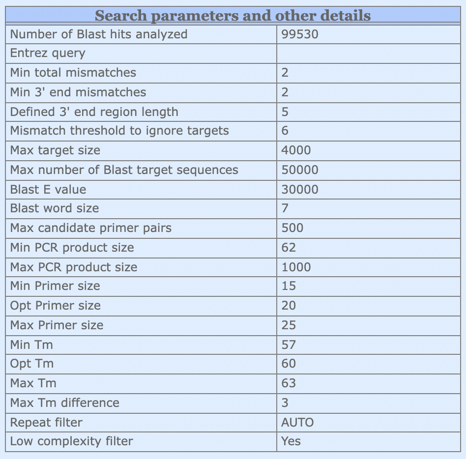
Figure 17: BLAST search parameters and other details.

Note: Performing Primer-BLAST analysis of the primer pairs obtained by deep-C-VAE model on the NCBI website. There are some parameters that need to be set before performing BLAST to ensure the validity of the analysis.

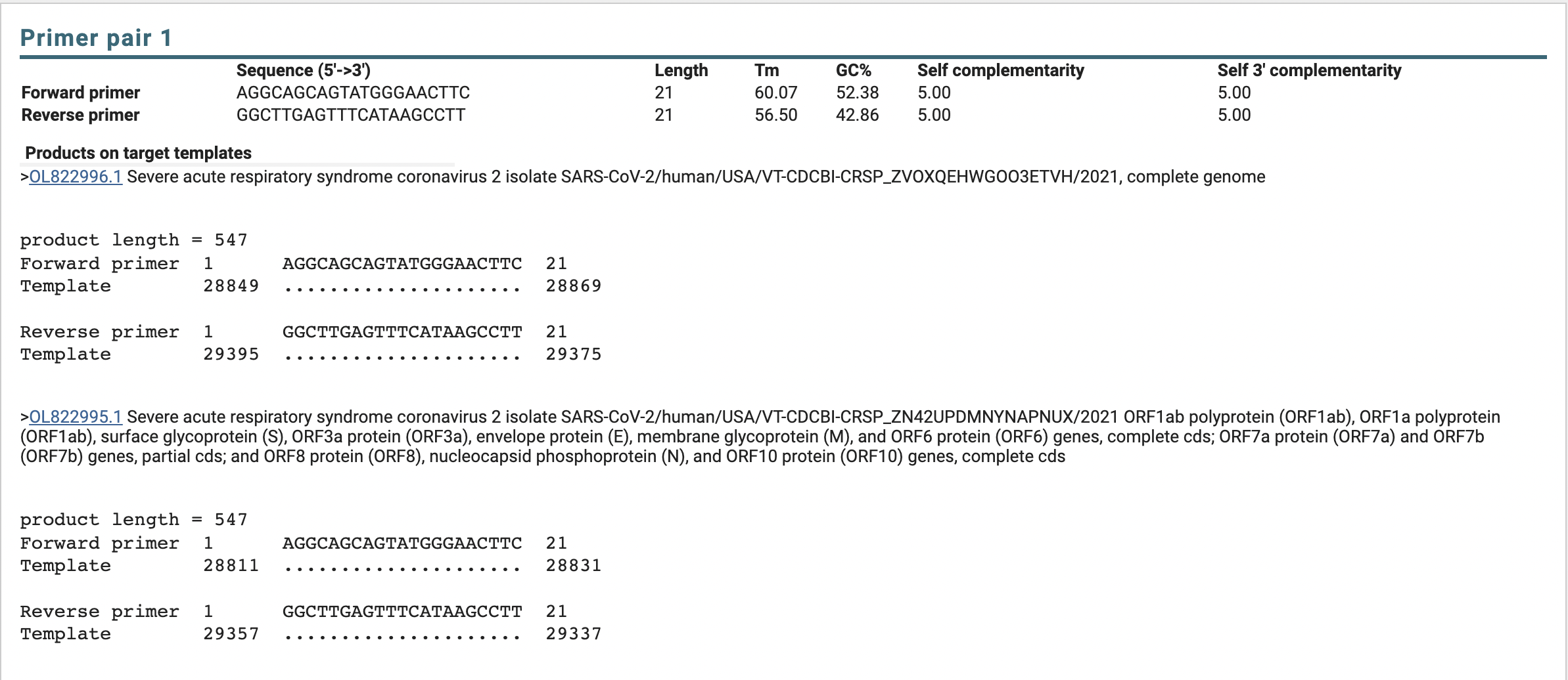
Figure 18: Snapshot of primer specificity checks using Primer-BLAST.

Note: This is the result of a Primer-BLAST completed on a primer pair, showing the Accession_ID and species of the gene sequence for which the primer pair could be searched, and the amplicon size of the PCR performed in that gene sequence using this primer pair.

In this section, the Fig 19 and Fig 20 show the result of in-silico PCR by using FastPCR software and Unipro UGENE software.

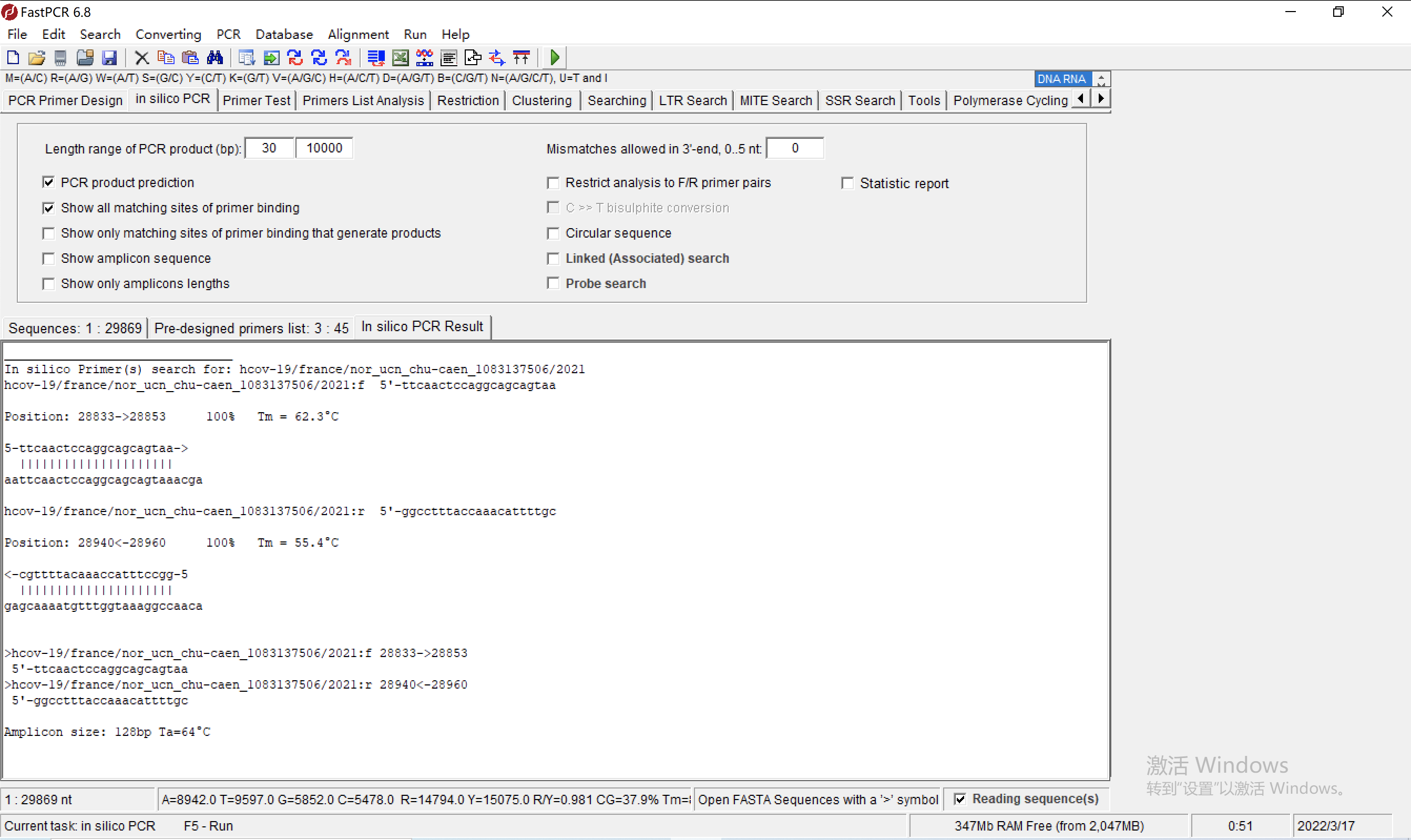
Figure 19: Snapshot of in-silico PCR analysis of chosen primer pairs using FastPCR software.

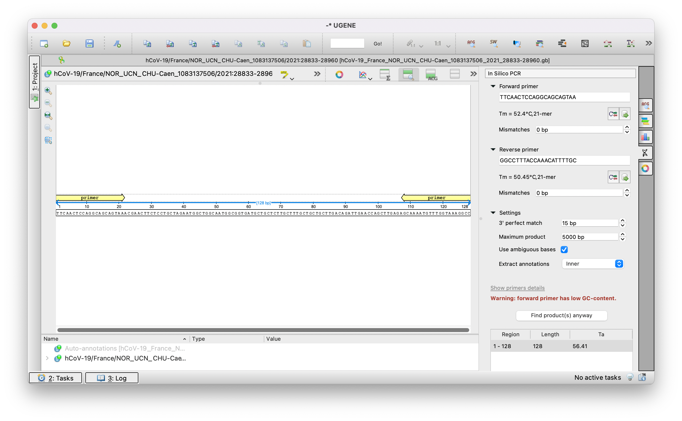
Figure 20: Snapshot of in-silico PCR analysis of pre-selected primer pairs using the Unipro UGENE software.

Appendix E Compare with Primer3Plus

In this section, the Table 16 shows the result of primer pairs generated by using our deep-learning method for both the forward and reverse primers and compare it with the result using Primer3Plus.

	Deep-learning Method		Primer3Plus
	(Flexible with no upper limit)		(Up to 10000 base pairs)
Forward Primer
Total at the beginning	3,626 primers		30 primers
GC content check	2,725 primers	$\downarrow$24.85%	30 primers	$\downarrow$0%
Frequency of appearance check	29 primers	$\downarrow$98.94%	0 primers	$\downarrow$100%
Reverse Primer
Total at the beginning	53,777 primers		30 primers
GC content check	34,955 primers	$\downarrow$35%	30 primers	$\downarrow$0%
Frequency of appearance check	357 primers	$\downarrow$98.98%	0 primers	$\downarrow$100%
Primer Pairs
Primer Design Rules	143 primer paris		0 primer pairs

Table 16: The comparison with the primer results of deep-learning method and Primer3Plus

Note: Since Primer3Plus can only input sequences of up to 10,000 base pairs at one time and generates 10 primer pairs (10 forward + 10 reverse) for every input. For a SARS-CoV-2 virus with an average length of 30,000 base pairs, the sequence needs to be divided into 3 segments and input separately, resulting in a total of 30 primer pairs.

References

- [1] Stephen Bustin and Jim Huggett. qPCR primer design revisited. Biomolecular Detection and Quantification, 14:19–28, 2017.
- [2] World Health Organization. Genomic sequencing of SARS-CoV-2: a guide to implementation for maximum impact on public health. https://www.who.int/publications/i/item/9789240018440, 2021. Accessed: 2024-10-11.
- [3] Illumina, Inc. Key differences between next-generation sequencing and sanger sequencing. https://emea.illumina.com/science/technology/next-generation-sequencing/beginners/advantages/ngs-vs-sanger.html, Oct 2024. Accessed: 2024-10-11.
- [4] Illumina, Inc. Advantages of next-generation sequencing vs. qPCR. https://www.illumina.com/science/technology/next-generation-sequencing/beginners/advantages/ngs-vs-qpcr.html, Oct 2024. Accessed: 2024-10-11.
- [5] Theodore Johnson, Tanner Bishoff, Kaleb Kremsreiter, Austin Lebanc, and Macario Camacho. Diagnostic testing for COVID-19: systematic review of meta-analyses and evidence-based algorithms. The Medical Journal, (PB 8-21-01/02/03):50–59, 2021.
- [6] Todd C Lorenz. Polymerase chain reaction: basic protocol plus troubleshooting and optimization strategies. Journal of Visualized Experiments, (63):e3998, 2012.
- [7] Stephen Bustin, Reinhold Mueller, and Tania Nolan. Parameters for successful PCR primer design. In Methods in Molecular Biology, volume 2065, pages 5–22, 2020.
- [8] Matej Lexa, Jakub Horak, and Bretislav Brzobohaty. Virtual PCR. Bioinformatics, 17(1):192–193, 2001.
- [9] Jian Ye, George Coulouris, Irena Zaretskaya, Ioana Cutcutache, Steve Rozen, and Thomas L Madden. Primer-blast: a tool to design target-specific primers for polymerase chain reaction. BMC Bioinformatics, 13(1):1–11, 2012.
- [10] Triinu Koressaar and Maido Remm. Enhancements and modifications of primer design program Primer3. Bioinformatics, 23(10):1289–1291, 2007.
- [11] Andreas Untergasser, Ioana Cutcutache, Triinu Koressaar, Jian Ye, Brant C Faircloth, Maido Remm, and Steven G Rozen. Primer3—new capabilities and interfaces. Nucleic Acids Research, 40(15):e115–e115, 2012.
- [12] Daniel Ashlock, Kenneth Bryden, Steven Corns, Patrick Schnable, and Tsui-Jung Wen. Training finite state classifiers to improve PCR primer design. In 10th AIAA/ISSMO Multidisciplinary Analysis and Optimization Conference, page 4385, 2004.
- [13] Jain-Shing Wu, Chungnan Lee, Chien-Chang Wu, and Yow-Ling Shiue. Primer design using genetic algorithm. Bioinformatics, 20(11):1710–1717, 2004.
- [14] Alejandro Lopez Rincon, Carmina A Perez Romero, Lucero Mendoza Maldonado, Eric Claassen, Johan Garssen, Aletta D Kraneveld, and Alberto Tonda. Design of specific primer sets for SARS-CoV-2 variants using evolutionary algorithms. In Proceedings of the Genetic and Evolutionary Computation Conference, pages 982–990, 2021.
- [15] Alejandro Lopez-Rincon, Alberto Tonda, Lucero Mendoza-Maldonado, Daphne GJC Mulders, Richard Molenkamp, Carmina A Perez-Romero, Eric Claassen, Johan Garssen, and Aletta D Kraneveld. Classification and specific primer design for accurate detection of SARS-CoV-2 using deep learning. Scientific Reports, 11(1):1–11, 2021.
- [16] Yuelong Shu and John McCauley. GISAID: global initiative on sharing all influenza data – from vision to reality. Eurosurveillance, 22(13), 2017.
- [17] National Center for Biotechnology Information Bethesda (MD): National Library of Medicine (US). National center for biotechnology information (ncbi)[internet]. Available from: https://www.ncbi.nlm.nih.gov/, 1988. Accessed: 2024-10-06.
- [18] Jinny X Zhang, Boyan Yordanov, Alexander Gaunt, Michael X Wang, Peng Dai, Yuan-Jyue Chen, Kerou Zhang, John Z Fang, Neil Dalchau, Jiaming Li, et al. A deep learning model for predicting next-generation sequencing depth from DNA sequence. Nature Communications, 12(1):1–10, 2021.
- [19] Allen Chieng Hoon Choong and Nung Kion Lee. Evaluation of Convolutionary Neural Networks Modeling of DNA Sequences using Ordinal versus one-hot Encoding Method. bioRxiv, page 186965, 2017.
- [20] Vinod Nair and Geoffrey E Hinton. Rectified linear units improve restricted boltzmann machines. In Icml, 2010.
- [21] Diederik P Kingma and Jimmy Ba. Adam: a method for stochastic optimization. arXiv preprint arXiv:1412.6980, 2017.
- [22] Adam Paszke, Sam Gross, Francisco Massa, Adam Lerer, James Bradbury, Gregory Chanan, Trevor Killeen, Zeming Lin, Natalia Gimelshein, Luca Antiga, et al. PyTorch: an imperative style, high-performance deep learning library. Advances in Neural Information Processing Systems, 32, 2019.
- [23] Jonathon Shlens. Notes on Kullback-Leibler Divergence and likelihood. arXiv preprint arXiv:1404.2000, 2014.
- [24] CW Dieffenbach, TM Lowe, and GS Dveksler. General concepts for PCR primer design. PCR Methods and Applications, 3(3):S30–S37, 1993.
- [25] Addgene: how to design primers. https://www.addgene.org/protocols/primer-design/, 2019. Accessed: 2024-10-30.
- [26] Rosario San Millán Joseba Bikandi. Melting temperature (tm) calculation. http://insilico.ehu.es/tm.php?formula=basic, July 2015. Accessed: 2024-10-30.
- [27] Integrated DNA Technologies. OligoAnalyzer Tool - Primer analysis and Tm calculator. https://eu.idtdna.com/pages/tools/oligoanalyzer. Accessed: 2024-10-22.
- [28] Livia Schrick and Andreas Nitsche. Pitfalls in PCR troubleshooting: expect the unexpected? Biomolecular Detection and Quantification, 6:1–3, 2016.
- [29] Ruslan Kalendar, Bekbolat Khassenov, Yerlan Ramankulov, Olga Samuilova, and Konstantin I Ivanov. FastPCR: an in silico tool for fast primer and probe design and advanced sequence analysis. Genomics, 109(3-4):312–319, 2017.
- [30] Konstantin Okonechnikov, Olga Golosova, Mikhail Fursov, and UGENE team. Unipro UGENE: a unified bioinformatics toolkit. Bioinformatics, 28(8):1166–1167, 2012.
- [31] Rui Wang, Jiahui Chen, Yuta Hozumi, Changchuan Yin, and Guo-Wei Wei. Emerging vaccine-breakthrough SARS-CoV-2 variants. ACS Infectious Diseases, 8(3):546–556, 2022. PMID: 35133792.
- [32] Paul A Christensen, Randall J Olsen, S. Wesley Long, Sishir Subedi, James J Davis, Parsa Hodjat, Debbie R Walley, Jacob C Kinskey, Matthew Ojeda Saavedra, Layne Pruitt, Kristina Reppond, Madison N Shyer, Jessica Cambric, Ryan Gadd, Rashi M Thakur, Akanksha Batajoo, Regan Mangham, Sindy Pena, Trina Trinh, Prasanti Yerramilli, Marcus Nguyen, Robert Olson, Richard Snehal, Jimmy Gollihar, and James M Musser. Delta variants of SARS-CoV-2 cause significantly increased vaccine breakthrough COVID-19 cases in Houston, Texas. The American Journal of Pathology, 192(2):320–331, 2022.
- [33] Xuemei He, Weiqi Hong, Xiangyu Pan, Guangwen Lu, and Xiawei Wei. SARS-CoV-2 Omicron variant: Characteristics and prevention. MedComm, 2(4):838–845, 2021.
- [34] World Health Organization. COVID-19 cases — WHO COVID-19 dashboard. https://data.who.int/dashboards/covid19/cases, Oct 2024. Accessed: 2024-10-11.
- [35] Prerna Arora, Christine Happle, Amy Kempf, Inga Nehlmeier, Metodi V Stankov, Alexandra Dopfer-Jablonka, Georg M N Behrens, Stefan Pöhlmann, and Markus Hoffmann. Impact of JN.1 booster vaccination on neutralisation of SARS-CoV-2 variants KP.3.1.1 and XEC. bioRxiv, 2024.10.04.616448, 2024. Available from: https://www.biorxiv.org/content/10.1101/2024.10.04.616448v1.
- [36] Fengxiang He, Tongliang Liu, and Dacheng Tao. Control batch size and learning rate to generalize well: theoretical and empirical evidence. Advances in Neural Information Processing Systems, 32:1143–1152, 2019.
- [37] Tal Schuster, Darsh J Shah, Yun Jie Serene Yeo, Daniel Filizzola, Enrico Santus, and Regina Barzilay. Towards debiasing fact verification models. arXiv preprint arXiv:1908.05267, 2019.
- [38] Áine O’Toole, Emily Scher, Anthony Underwood, Ben Jackson, Verity Hill, John T McCrone, Rachel Colquhoun, Chris Ruis, Khalil Abu-Dahab, Ben Taylor, Corin Yeats, Louis du Plessis, Daniel Maloney, Nathan Medd, Stephen W Attwood, David M Aanensen, Edward C Holmes, Oliver G Pybus, and Andrew Rambaut. Assignment of epidemiological lineages in an emerging pandemic using the pangolin tool. Virus Evolution, 7(2), 2021. veab064.
- [39] Geoffrey E Hinton and Sam Roweis. Stochastic neighbor embedding. Advances in Neural Information Processing Systems, 15:1–8, 2002.
- [40] Matthew A Croxen, Robyn J Law, Roland Scholz, Kristie M Keeney, Marta Wlodarska, and B. Brett Finlay. Recent advances in understanding enteric pathogenic Escherichia coli. Clinical Microbiology Reviews, 26(4):822–880, 2013.
- [41] Elaine Scallan, Robert M Hoekstra, Frederick J Angulo, Robert V Tauxe, Marc-Alain Widdowson, Sharon L Roy, Jeffery L Jones, and Patricia M Griffin. Foodborne illness acquired in the United States–major pathogens. Emerging Infectious Diseases, 17(1):7–15, 2011.
- [42] Dirk Wildeboer, Linda Amirat, Robert G Price, and Ramadan A Abuknesha. Rapid detection of Escherichia coli in water using a hand-held fluorescence detector. Water Research, 44(8):2621–2628, 2010.
- [43] Ying Chen, Linyan Zhang, Ling Xu, Xinjian Guo, Huan Yang, Linlin Zhuang, Ying Li, Zhenzhen Wang, and Bing Gu. Rapid and sensitive detection of Shigella flexneri using fluorescent microspheres as label for immunochromatographic test strip. Annals of Translational Medicine, 7(20):565, 2019.
- [44] Chantal BF Vogels, Mallery I Breban, Isabel M Ott, Tara Alpert, Mary E Petrone, Anne E Watkins, Chaney C Kalinich, Rebecca Earnest, Jessica E Rothman, Jaqueline Goes de Jesus, Ingra Morales Claro, Giulia Magalhães Ferreira, Myuki AE Crispim, Brazil-UK CADDE Genomic Network, Lavanya Singh, Houriiyah Tegally, Ugochukwu J Anyaneji, Network for Genomic Surveillance in South Africa, Emma B Hodcroft, Christopher E Mason, Gaurav Khullar, Jessica Metti, Joel T Dudley, Matthew J MacKay, Megan Nash, Jianhui Wang, Chen Liu, Pei Hui, Steven Murphy, Caleb Neal, Eva Laszlo, Marie L Landry, Anthony Muyombwe, Randy Downing, Jafar Razeq, Tulio de Oliveira, Nuno R Faria, Ester C Sabino, Richard A Neher, Joseph R Fauver, and Nathan D Grubaugh. Multiplex qPCR discriminates variants of concern to enhance global surveillance of SARS-CoV-2. PLoS Biology, 19(5):e3001236, 2021.
- [45] Mamdouh Sibai, Hannah Wang, Priscilla SW Yeung, Malaya K Sahoo, Daniel Solis, Kenji O Mfuh, ChunHong Huang, Fumiko Yamamoto, and Benjamin A Pinsky. Development and evaluation of an RT-qPCR for the identification of the SARS-CoV-2 Omicron variant. Journal of Clinical Virology, 148:105101, 2022.
- [46] Hannah Wang, Jacob A Miller, Michelle Verghese, Mamdouh Sibai, Daniel Solis, Kenji O Mfuh, Becky Jiang, Naomi Iwai, Marilyn Mar, ChunHong Huang, Fumiko Yamamoto, Malaya K Sahoo, James Zehnder, and Benjamin A Pinsky. Multiplex SARS-CoV-2 genotyping reverse transcriptase PCR for population-level variant screening and epidemiologic surveillance. Journal of Clinical Microbiology, 59(8):e00859–21, 2021.