Self-Adaptive Gamma Context-Aware SSM-based Model for Metal Defect Detection

Abstract

Metal defect detection is critical in industrial quality assurance, yet existing methods struggle with grayscale variations and complex defect states, limiting its robustness. To address these challenges, this paper proposes a Self-Adaptive Gamma Context-Aware SSM-based model(GCM-DET). This advanced detection framework integrating a Dynamic Gamma Correction (GC) module to enhance grayscale representation and optimize feature extraction for precise defect reconstruction. A State-Space Search Management (SSM) architecture captures robust multi-scale features, effectively handling defects of varying shapes and scales. Focal Loss is employed to mitigate class imbalance and refine detection accuracy. Additionally, the CD5-DET dataset is introduced, specifically designed for port container maintenance, featuring significant grayscale variations and intricate defect patterns. Experimental results demonstrate that the proposed model achieves substantial improvements, with mAP@0.5 gains of 27.6%, 6.6%, and 2.6% on the CD5-DET, NEU-DET, and GC10-DET datasets.

^∗Equal contribution  ^†Corresponding author

1 Introduction

The quality of metal surfaces is critical in various industrial applications, including aerospace, manufacturing, and container transportation. Surface defects, such as cracks, dents, and scratches, not only compromise the structural integrity and aesthetics of metal products but also lead to significant economic losses if left undetected. As a result, the accurate and efficient detection of metal surface defects has become an essential task in industrial quality control.

In recent years, the adoption of deep learning techniques has significantly advanced the performance of defect detection systems[1]. Convolutional neural networks (CNNs) and transformer-based models have demonstrated exceptional capabilities in handling complex image-based tasks, enabling automated and reliable defect detection. However, several challenges remain: 1) Metal defect often exhibits varied and localized features, making effective multi-scale feature aggregation vital for improving detection accuracy. 2) The boundary features of damaged areas are typically irregular and complex. 3) Extreme recognition bias due to environment and perspective. Existing feature sampling methods, particularly attention mechanisms, often struggle with adequate spatial representation.

To address these challenges, this paper proposes novel improvements in two key modules of the defect detection pipeline, enhancing both the precision and robustness of detection methods. Inspired by the CARAFE[2] upsampling method, a gamma coefficient down-correction module based on dynamic coefficients is proposed. The state space search model[3] reconstructs the weights of the feature map through content perception to obtain the deep features of the model. Then, the F-Loss[4] is introduced to weigh the indicators between single weights and global weights.

Furthermore, CD5-DET is designed for container damage detection, containing a diverse set of labeled images that capture 5 defect types under varying environmental conditions. The dataset bridges a critical gap in the field by providing a standardized benchmark for defect detection in industrial settings.

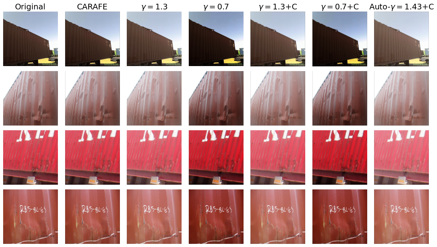
Figure 1: The original image may have exposure, shadows, etc. When capturing features, using different Gamma $\gamma$ coefficients for different situations can improve the quality of the image. Multiplying each pixel value of an image by $\gamma$ represents a linear scaling transformation of the pixel values of the image. Using constant defined Gamma coefficients (greater than 1 can make the image brighter, while less than 1 can make the image darker) can change the features of the image for specific situations. It can be found that the visibility of the processed image is significantly improved.

The main contributions of this study can be summarized as followings:

1. This paper proposes a upsampling structure combined with a dynamic gamma coefficient. Before cascade module upsampling, the adaptive gamma coefficient correction is used to provide generalization for the feature map and effectively collect model features.

2. This paper proposes a GCM-DET model based on the State-space search architecture. The SSM architecture is used to improve the backbone and neck of the model. The new improvements are SSM-Backbone and SSM-Neck. The improved model improves the feature fusion capability of the backbone architecture.

3. This work collected and developed the industry’s first container damage dataset CD5-DET, and then obtained excellent indicators on the well-known defect detection datasets NEU-DET and GC10-DET. Experimental results show that the GCM-DET model under the SSM architecture can effectively extract visual features of images and provide excellent robustness on related tasks.

2 Related Work

Several metal defect detection datasets have already been applied to academic research. The most commonly used ones are NEU-DET[5] and GC10-DET[6], while baseline models include YOLO series, Faster-RCNN, U-Net and other model structures. Generally speaking, metal defect detection uses an engineering computer with a camera to collect images. Then, the processed image is input into the target detection algorithm[7]. Similarly, applied to the topic of container defect detection, a model is designed for detecting container defects, which was applied to port cameras after evaluation and deployed. Therefore, designing an efficient algorithm and organizing excellent datasets play an important role in the field of target detection.

2.1 Defect Detection

Considering the different sizes and shapes of metal surface defects, previously detection models[8] use multi-scale detection heads to provide a rich receptive field for the model. Small detection heads provide local parameters for the model, and large detection heads provide the shape and contour of the template for the model. At present, the mainstream research methods are mainly considered from three perspectives: machine learning methods and deep learning methods.

2.2 Machine Learning Method

Early defect detection methods mainly used machine learning models. In Wang’s study, a model combining HOG-LBP[9] was used to provide the best detection performance on the INRIA dataset. Song’s study[5] enhanced the processing of noise by optimizing the LBP method, and then used the SVM method to classify the defect results. In addition, Li et al. proposed the SURF method[10] to replace the Haar[11] classifier for target detection. These methods use the concept of manual features and statistical prior knowledge to achieve high accuracy in simple target detection tasks.

2.3 Deep Learning Method

Thanks to the development of computer vision technology, many deep learning visual tasks have been improved to target detection tasks. At present, the mainstream deep learning methods are mainly divided into two-step detection and single-step detection methods. For the two-step selection method, first, the detection head generates target candidate boxes. Then it is connected to the target classification algorithm classifier. Common two-stage detection algorithms include RCNN[12], Fast-RCNN[13] and Mask-RCNN[14]. Single-stage target detection algorithms perform dense target detection directly on the input image without generating candidate regions. They usually use convolutional neural networks (CNN) to detect and classify targets on feature maps, and then fine-tune the position of the detection box to accurately locate the object. Common single-stage algorithms include the YOLO series[15]. Deep learning-based methods can automatically learn high-level features from training data and effectively capture hidden features inside the image. Compared with traditional defect detection methods, they are not only suitable for complex environments and different tasks, but also can provide accurate and fast recognition results.

As a result of YOLO’s excellent feature capture capabilities, many scholars have conducted research and improvements based on the YOLO method.

Woo et al. proposed the CMAM module [16] to replace the CNN module for inferring channel attention and spatial attention. The lightweight SE attention method [17] uses efficient multi-scale attention (EMA) to improve the accuracy of target detection while reducing the number of network parameters. In addition, ViTransformer [18] studies the fusion of the visual backbone architecture of self-attention and the weighted bidirectional feature pyramid network (BiFPN) to achieve better accuracy and robustness. Many scholars have studied how to reduce the number of parameters of yolo to improve the frame rate (FPS). Shufflenet [19] uses point-by-point group convolution and channel shuffling methods to improve operating efficiency by about 13x. The Google team proposed the MobileNet network [20], which combines the deep convolution and point-by-point convolution methods, uses the width operator to control the number of channels in each layer of the network, further balances the size and performance of the model, and uses the resolution multiplier to adjust the resolution of the input image, affecting the size and computation of the feature map. The use of Ghost module[21] replaces the feature extraction module in the yolo backbone network, effectively accelerating the calculation process.

Proposed work compares with the above models under identical training settings to highlight the superior multi-scale representation which this method achieves.

3 Methodology

3.1 Detection Framework

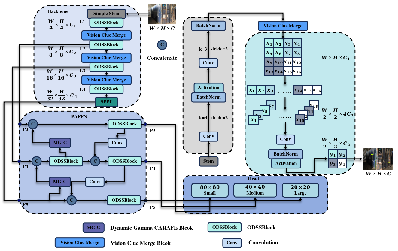
Figure 2: Proposed framework includes a Dynamic Gamma Block, where the Gam-Car model applies adaptive Gamma correction to the original image based on variations in $\mu$ and $\sigma$, while the Pix-shuffling provides super-resolution sampling for image scaling. An ODSS Block and a Vision Clue Merge Block are employed to further enhance the image processing.

YOLO series models are the mainstream methods of target detection. Relevant research shows that the YOLOv8 series[22] model has better performance and indicators than previous models in related detection tasks. Considering the balance between accuracy and computing speed, YOLOv8n is used as the backbone model. Although the ViT model based on the attention mechanism significantly improves the special diagnosis map in the backbone, the multiple calculation mechanism of the self-attention model brings heavy computational efficiency to the structure. Visual State Space Model [3] is introduced to alleviate exponential computational complexity. In addition, considering the noisy images and low-resolution features in the real environment, Gamma-Carafe structure is used to replace the upsampling layer in the original YOLOv8 backbone architecture. In addition, the introduction of Focal-IoU loss function solves the dynamic factor differences of overlapping area, center point and side length. Combining these methods, the detection framework is designed as shown in Figure-2.

3.2 Proposed GCM-DET

3.2.1 Gamma-Carafe

Inspired by the CARAFE (Content-Aware ReAssembly of FEatures) structure, this work introduces dynamic grayscale correction to replace the original interpolation upsampling layer of the baseline model. CARAFE is a content-aware upsampling method that reorganizes input features by generating dynamic convolution kernels, making the reconstructed high-resolution feature map more accurate. In addition, dynamic Gamma processing optimizes the robustness input of the model.

Improved Gam-Car model is added a dynamic search gamma method before implementing CARAFE. In order to reduce the model’s dependence on the grayscale of the image, dynamically adjusting the model’s brightness coefficient can increase the model’s ability to capture deep features.

The implementation of Gamma-Carafe mainly consists of three steps: 1) Optimize the grayscale features of the model; 2) Generate predicted reassembly kernels; 3) Reassemble kernel features.

Dynamic Gamma Correction

This algorithm adjusts image brightness dynamically by employing a Gamma correction that is computed based on the image’s brightness characteristics. First, the input RGB image tensor $x$ is converted to grayscale to derive brightness information. This grayscale brightness is calculated using the weighted sum Equation-1:

$$gray=0.299\cdot R+0.587\cdot G+0.114\cdot B$$ (1)

, where $R$, $G$, and $B$ represent the red, green, and blue channels, respectively.

To adaptively determine the Gamma value, the mean and standard deviation of the brightness are calculated for each image in the batch. These values are used to modulate Gamma dynamically:

$$\gamma=G_{min}+(G_{max}-G_{min})\cdot\frac{gray_{mean}}{gray_{mean}+gray_{std}+\epsilon}$$ (2)

where $\epsilon$ is a small constant to prevent division by zero. The resulting Gamma value is clamped to ensure it remains within the pre-defined range $[G_{min},G_{max}]$.

Finally, the calculated Gamma is applied to each pixel of the image by raising the pixel values (incremented by a small value $\epsilon$) to the power of Gamma, normalizing the brightness without exceeding the valid range $[0,1]$. This dynamic approach allows the algorithm to adjust the image brightness more effectively, reducing reliance on grayscale characteristics alone and enhancing feature retention. The affections of different $\gamma$ can be seen in Figure-1.

Kernel Prediction.

For kernel prediction, the purpose of this module is to predict the appropriate convolution kernel $W_{l^{\prime}}$. By predicting the adjacent region $N(X_{l},k_{\text{encoder}})$ in position $l^{\prime}$, it can be calculated:

$$\mathcal{W}_{l^{\prime}}=\psi(N(\mathcal{X}_{l},k_{encoder}))$$ (3)

The Equation-3 generates an adaptive convolution kernel based on the input feature content, which is used to dynamically reorganize the features. Here $N(X_{l},k_{\text{encoder}})$ represents the information of the input feature $X_{l}$ in the neighborhood of the convolution kernel size $k_{\text{encoder}}$.

Feature Reassembly.

Use $\psi$ to infer the adaptive convolution kernel $W_{l^{\prime}}$, and resample the features through $N(X_{l},k_{\text{up}})$, expressed as:

$$X^{\prime}_{l^{\prime}}=\phi(N(X_{l},k_{\text{up}}),W_{l^{\prime}})$$ (4)

The Equation-4 uses the content-aware convolution kernel to reorganize input features, so that the upsampling process can be adaptively adjusted according to the content at different locations, thus improving upsampling accuracy and feature expression ability. The steps of feature reorganization are as follows.

Channel Compression.

The module performs channel compression on the input features, and compresses the number of input channels $c$ to the number of intermediate channels $c_{\text{mid}}$ through convolution operation:

$$F_{\text{comp}}(x)=W_{\text{comp}}*x+b_{\text{comp}}$$ (5)

Where $W_{\text{comp}}$ is the convolution kernel used for compression, $b_{\text{comp}}$ is the bias term, and * indicates the convolution operation. This operation compresses the number of feature channels from $c$ to $c_{\text{mid}}$.

Content Encoder.

Next, a convolution layer is used to generate the upsampling kernel. The size of the generated convolution kernel is $(scale\times k_{\text{up}})^{2}$, where $scale$ is the upsampling factor and $k_{\text{up}}$ is the kernel size used for upsampling. This process is expressed by the following equation:

$$F_{\text{enc}}(x)=W_{\text{enc}}*F_{\text{comp}}(x)$$ (6)

$W_{\text{enc}}$ is the weight used to generate the convolution kernel. The dimension of the output $F_{\text{enc}}(x)$ is $(scale\times k_{\text{up}})^{2}$.

Pixel Normalization.

After the generated convolution kernel, the pixel shuffling operation is used to rearrange the generated feature map into a high-resolution map. Assume that the input feature map is $F_{\text{in}}\in\mathbb{R}^{H\times W\times C}$, where $C=C_{\text{out}}\times r^{2}$. The PixelShuffle process can be expressed as:

The PixelShuffle operation re-arranges the input channels so that the feature map resolution is increased by the upsampling factor.

Finally, combining convolution kernel perception and feature reorganization by Equation-8.

$$\mathcal{X}_{l^{\prime}}^{\prime}=\sum_{n=-r}^{r}\sum_{m=-r}^{r}\mathcal{W}_{l^{\prime}(n,m)}\cdot\mathcal{X}_{(i+n,j+m)}$$ (8)

3.2.2 State Space Model

The structured state space models (S4)[23] and Mamba[24], as instances of State Space Model (SSM), are derived from continuous systems. These models map a one-dimensional input function or sequence $x(t)\in\mathbb{R}$ to an output $y(t)\in\mathbb{R}$ thought a hidden state $h(t)\in\mathbb{R}^{N}$. The evolution parameter $A\in\mathbb{R}^{N\times N}$ and projections parameters $B\in\mathbb{R}^{N\times 1}$ , $C\in\mathbb{R}^{1\times N}$ are used in this system.

$$h^{\prime}(t)=\mathbf{A}h(t)+\mathbf{B}x(t)$$ (9)

$$y(t)=\mathbf{C}h(t)$$ (10)

S4 and Mamba are discrete versions of the continuous system. They use a timescale parameter $\Delta$ to discretize the continuous parameters $A$ and $B$ into $\bar{A}$ and $\bar{B}$. The commonly used method for this transformation is zero-order hold (ZOH), which is defined as follows:

$$\bar{\mathbf{A}}=\exp(\Delta\mathbf{A})$$ (11)

$$\bar{\mathbf{B}}=(\Delta\mathbf{A})^{-1}\left(\exp(\Delta\mathbf{A})-\mathbf{I}\right)\Delta\mathbf{B}$$ (12)

After discretizing the parameters into $\bar{A}$ and $\bar{B}$ with a step size of $\Delta$, the Equations- [9,10] can be rewritten as:

$$h_{t}=\bar{\mathbf{A}}h_{t-1}+\bar{\mathbf{B}}x_{t}$$ (13)

$$y_{t}=\mathbf{C}h_{t}$$ (14)

Finally, the model computes the output through a global convolution.

$$\bar{\mathbf{K}}=(\mathbf{C}\bar{\mathbf{B}},\mathbf{C}\bar{\mathbf{A}}\bar{\mathbf{B}},\ldots,\mathbf{C}\bar{\mathbf{A}}^{L-1}\bar{\mathbf{B}})$$ (15)

$$y=x*\bar{\mathbf{K}}$$ (16)

Where $\bar{K}\in\mathbb{R}^{L}$ is the structured convolutional kernel, and $L$ is the length of the input sequence $x$.

Mamba-YOLO[25] can be referred to as Figure-2, Mamba-YOLO replaces the backbone with ODMamba, which consists of a Simple Stem using two convolutions with a stride of 2 and a kernel size of 3, along with a downsampling module. The neck follows the PAN-FPN design, using the ODSSBlock module to replace C2f[26], where Conv is solely responsible for downsampling. The backbone first performs downsampling through the Stem module.The Stem module uses two convolution operations with a stride of 2 and a kernel size of 3, generating a 2D feature map with a resolution of $H/4\times W/4$, followed by further downsampling through the Vision Clue Merge and ODSSBlock modules. The Vision Clue Merge module employs a method of splitting feature maps and using 1x1 convolutions to reduce dimensions while retaining more visual clues, thereby optimizing the training of State Space Models (SSMs). By removing normalization, splitting the dimension maps, and utilizing 4x compressed pointwise convolutions, it simplifies the processing flow while preserving more critical feature information, enhancing the model’s performance and efficiency. ODSSBlock as shown in the Figure-3.

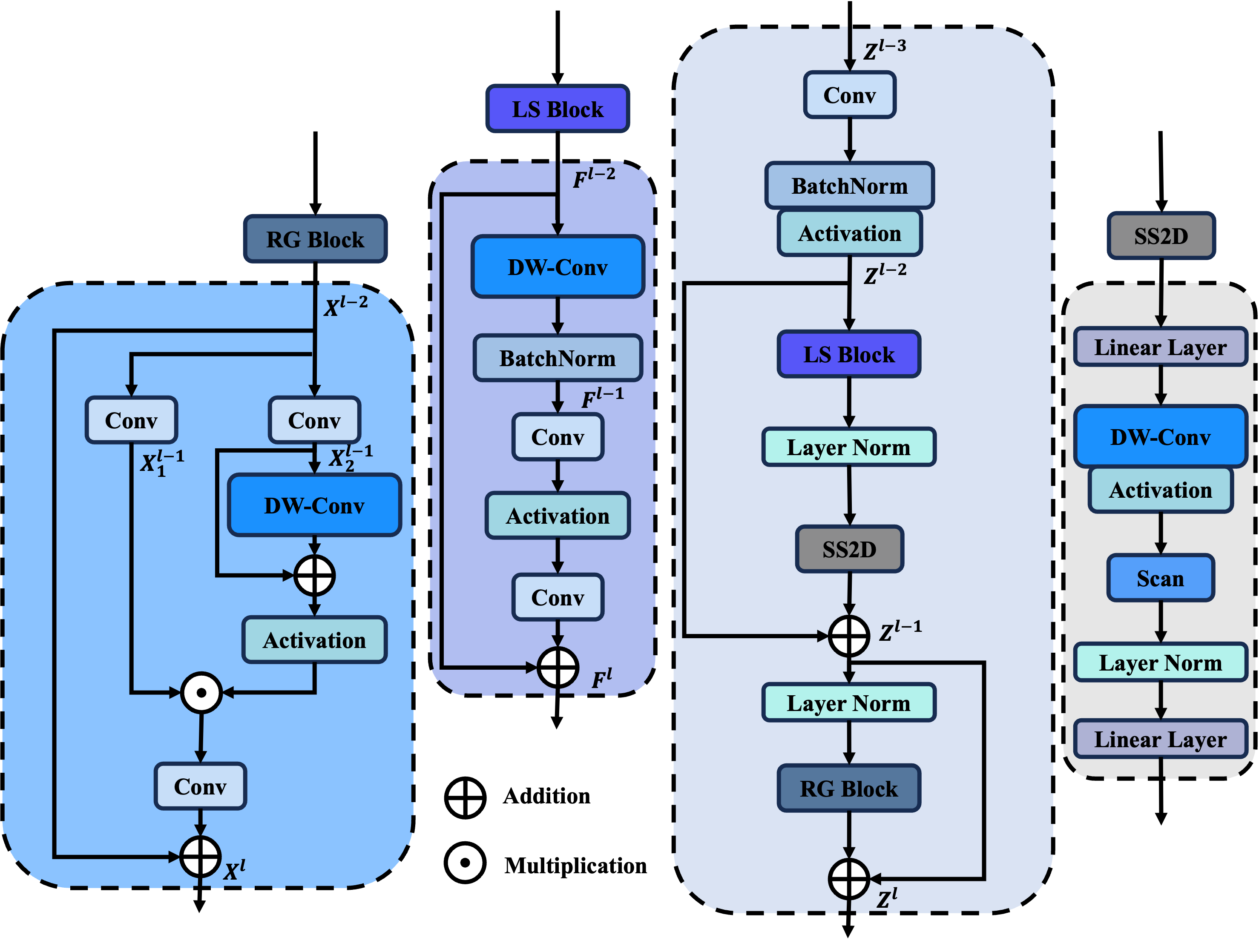
Figure 3: ODSSBlock

ODSSBlock performs a series of processes in the input stage, while maintaining efficiency and stability in the training and inference process through batch normalization.

Compared with standard convolution or attention mechanisms, the state-space formulation can model long-range spatial interactions and subtle local features simultaneously. By discretizing the continuous state evolution with a suitable $\Delta$, the SSM captures spatiotemporal dependencies inherent in textures and edges. This is particularly beneficial for complex defect shapes where boundary irregularities demand a more global yet flexible representation. For instance, when detecting random corrosion spots, the structured convolution kernel derived by SSM can adapt to changing patterns without inflating computational costs, thereby retaining both global context and minute details.

$$Z^{l-2}=\hat{\Phi}(BN(Conv_{1\times 1}(Z^{l-3})))$$ (17)

Where $\hat{\Phi}$ represents the activation function (nonlinear SiLU), inspired by the architecture style of Transformer Blocks [27], the ODSSBlock incorporates layer normalization and residual connections. The equations are as follows:

$$Z^{l-1}=SS2D(LN(LS(Z^{l-2})))+Z^{l-2}$$ (18)

$$Z^{l}=RG(LN(Z^{l-1}))+Z^{l-1}$$ (19)

Where LS and RG represent LocalSpatial Block and ResGated Block, respectively, $Z^{l-3}$ and $Z^{l}$ denote the input and output features, and $Z^{l-1}$ represents the intermediate state after 2D-Selective-Scan (SS2D [28]).

LocalSpatial Block is used to enhance the capture of local features. First, depth-separable convolution is applied to the given input feature $F^{l-1}\in\mathbb{R}^{C\times H\times W}$, operating independently on each input channel without mixing the channel information to effectively extract the local spatial information of the input feature map, while simultaneously reducing computational cost and the number of parameters. Then, Batch Normalization is performed to provide regularization and avoid overfitting. The resulting intermediate state $F^{l-1}$ is defined as:

$$F^{l-1}=BN(DWConv_{3\times 3}(F^{l-2}))$$ (20)

The intermediate state $F^{l-1}$ mixes the channel information through a 1×1 convolution, using the nonlinear GELU activation function to better preserve the information distribution.

$$F^{l}=Conv_{1\times 1}(\Phi(Conv_{1\times 1}(F^{l-1})))\oplus F^{l-2}$$ (21)

Where $F^{l}$ is the output feature, and $\Phi$ represents the activation function.

The RG Block creates two branches, $X_{1}^{l-1}$ and $X_{2}^{l-1}$, from the input $X^{l-2}$, and each branch implements a fully connected layer in the form of a 1x1 convolution.

$$X_{1}^{l-1}=\text{Conv}_{1\times 1}(X^{l-2})$$ (22)

$$X_{2}^{l-1}=\text{Conv}_{1\times 1}(X^{l-2})$$ (23)

The RG Block adopts a nonlinear GeLU as the activation function, followed by elemental multiplication to fuse with the $X_{2}^{l-1}$ branch, and a $1\times 1$ convolution to extract global features and blend channel information. Finally, the features in the hidden layer are added to the original input $X^{l-2}$ through residual connections. With only a slight increase in computational cost, the RG Block gains the ability to capture more global features, and the feature $X^{l}$ is defined as follows:

$$X^{l}=\text{Conv}_{1\times 1}(X_{1}^{l-1}\odot\Phi(\text{DWConv}_{3\times 3}(X_{2}^{l-1})\\ \oplus X_{2}^{l-1}))\oplus X^{l-2}$$ (24)

Where $\Phi$ denotes the activation function. The gating mechanism of the RG Block uses integrated convolution operations, preserving the spatial information in the image and making the model more sensitive to fine-grained features.

3.3 Focal Loss

With further optimize the bounding box regression accuracy of the object detection model, the Focal IoU loss is adopted, which aims to solve the problem that the traditional IoU (Intersection over Union) loss is insensitive to difficult samples (such as small objects and occluded objects) in detection tasks. Focal IoU introduces a dynamic weight mechanism to improve the regression effect of the model by amplifying the contribution of difficult-to-predict samples to the loss.

In the standard IoU loss, the model calculates the intersection over union ratio between the predicted box and the true box. However, this loss function is often difficult to effectively optimize small objects and highly overlapping objects when dealing with complex scenes. In particular, when the IoU between the predicted box and the true box is large, the standard IoU loss is less sensitive to position fine-tuning, making it difficult to further optimize the model. Focal IoU introduces a dynamic weight mechanism to give higher weights to difficult samples with smaller IoU, ensuring that the model focuses on these samples during training, thereby improving regression accuracy.

Specifically, the calculation process of Focal Loss is as follows:

Calculate the IoU value of the predicted bounding box and the true bounding box.

The IoU (Intersection over Union) calculation Equation of the predicted box $B_{p}$ and the true box $B_{g}$ is:

$$\text{IoU}(B_{p},B_{g})=\frac{|B_{p}\cap B_{g}|}{|B_{p}\cup B_{g}|}$$ (25)

Among them, $|B_{p}\cap B_{g}|$ represents the intersection area of the predicted box and the true box, and $|B_{p}\cup B_{g}|$ represents the union area of the two.

Divide samples according to the size of IoU value.

According to the IoU value, divide the samples into high-quality samples and low-quality samples. The classification criteria can be customized, and a threshold $\text{IoU}_{\text{thresh}}$ can usually be set:

$$\sigma=\begin{cases}\text{If}\ \text{IoU}(B_{p},B_{g})\geq\text{IoU}_{\text{thresh}},\ \text{high-quality}\\ \text{If}\ \text{IoU}(B_{p},B_{g})<\text{IoU}_{\text{thresh}},\ \text{low-quality}\end{cases}$$ (26)

Introduce adjustment factor $\alpha$.

Introduce adjustment factor $\alpha$ to balance the contribution of high-quality samples and low-quality samples to the loss. The value range of the adjustment factor is $0\leq\alpha\leq 1$, and the equation is as follows:

$$\alpha=\begin{cases}\alpha_{\text{high}}&\text{if IoU}(B_{p},B_{g})\geq\text{IoU}_{\text{thresh}}\\ \alpha_{\text{low}}&\text{if IoU}(B_{p},B_{g})<\text{IoU}_{\text{thresh}}\end{cases}$$ (27)

Among them, $\alpha_{\text{high}}$ and $\alpha_{\text{low}}$ are the weight factors of high-quality and low-quality samples respectively.

Calculate the loss of high-quality and low-quality samples.

For high-quality samples, the standard IoU loss is used directly:

$$\mathcal{L}_{\text{IoU}}=1-\text{IoU}(B_{p},B_{g})$$ (28)

For low-quality samples, the loss is scaled by the adjustment factor:

$$\mathcal{L}_{\text{low}}=\alpha_{\text{low}}\cdot(1-\text{IoU}(B_{p},B_{g}))^{\gamma}$$ (29)

Among them, $\gamma$ is an adjustable parameter used to control the impact of low-quality samples on the loss.

Weighted sum to get the final Focal IoU Loss.

The final Focal IoU Loss is the weighted sum of all sample losses, and the Equation is:

$$\mathcal{L}_{\text{Focal IoU}}=\sum_{i=1}^{N}\alpha_{i}\cdot(1-\text{IoU}(B_{p,i},B_{g,i}))^{\gamma}$$ (30)

Where $N$ represents the number of samples, $\alpha_{i}$ is the weight of the $i$th sample, and $\text{IoU}(B_{p,i},B_{g,i})$ represents the IoU of the $i$th sample.

4 Experiment

4.1 Datasets Preparation

In this study, for container defect detection, the CD5-DET (will publish after double-blind) is used, which contains deframe, hole, minior_dent, major_dent and rust. There are about 150 images in each class, and a total of 800 images are used in the entire dataset. In addition, NEU-DET[5] and GC10-DET[6] are collected for generalization experiments and ablation experiments.

4.2 Experimental Environment

A host machine is operated with Docker virtualization for the experiment with RTX-4090. The batch size is set to 16, the initial learning rate is set to 0.01, and the training cycle is set to 300. All input image data are uniformly processed to an input image size of 640 × 640. The dataset is divided according to the default ratio published by the corresponding author.

Table 1: Comparison Study on CD5-DET

Method	AP@0.5					mAP@0.5	mAP@0.5:0.95	Params(M)	GFLOPs	Size(Mb)
	De.	Ho.	Ma.	Mi.	Ru.
YOLOv5n	0.257	0.589	0.199	0.054	0.155	0.251	0.119	2.5	7.1	5.0
YOLOv6n	0.177	0.552	0.133	0.006	0.073	0.188	0.082	4.2	11.8	8.3
YOLOv8n	0.336	0.548	0.183	0.069	0.151	0.257	0.132	3.0	8.1	6.0
YOLOv8s	0.503	0.656	0.281	0.151	0.283	0.375	0.203	11.1	28.4	21.4
YOLOv8l	0.428	0.594	0.247	0.190	0.339	0.360	0.191	43.6	165.4	166.9
YOLOv8-world	0.434	0.589	0.226	0.121	0.281	0.330	0.171	4.1	14.2	15.8
YOLOv8-worldv2	0.406	0.482	0.241	0.082	0.234	0.289	0.134	3.5	9.9	13.9
YOLOv8-ghost	0.404	0.549	0.256	0.054	0.146	0.282	0.138	1.7	5.1	3.6
YOLOv10n	0.128	0.500	0.125	0.039	0.092	0.177	0.081	2.7	8.4	10.8
YOLOv10s	0.259	0.548	0.288	0.101	0.196	0.278	0.177	8.1	24.8	31.3
YOLO-Mamba-B	0.600	0.568	0.382	0.316	0.376	0.448	0.246	21.8	49.7	41.9
YOLO-Mamba-T	0.415	0.595	0.361	0.106	0.274	0.350	0.173	6.1	14.3	11.7
YOLO-Mamba-L	0.436	0.542	0.325	0.245	0.372	0.485	0.284	57.6	156.2	110.5
GCM-DET(Ours)	0.660	0.590	0.430	0.386	0.596	0.533	0.374	21.8	49.7	83.9

4.3 Evaluation Metrics

Proposed study evaluates the performance of the model from two indicators: accuracy and complexity. Mainly, AP@T and mAP@T are used to evaluate the accuracy of the model respectively. The T parameters used more frequently are 50% and 50:95%. $mAP@0.5$ indicates that when the overlap between the position $g^{p}$ of the model’s prediction box and the true value box $g^{t}$ exceeds 50%, it can be considered that the model’s prediction result is the same as the actual value. mAP@50:95 is used for higher accuracy evaluation results. The calculation of AP and mAP is expressed as Equation-31,32.

$$AP\left(i\right)=\int_{0}^{1}P\left(R\right)\mathrm{d}R$$ (31)

$$mAP=\frac{\sum_{i=1}^{n}AP(i)}{n}$$ (32)

In addition, the number of parameters, GFLOPs, and model size are used to compare the computational complexity of the model. The number of parameters represents the number of trainable parameters, reflecting the spatial complexity of the model; GFLOPs (gigafloating-point operations per second) quantifies the amount of computation required by the model, reflecting the time complexity; and the model size indicates the memory usage, reflecting the storage requirements when the model is deployed.

4.4 Comparison Study

By comparing multiple baseline YOLO models and additional World CLIP method. Proposed GCM-DET has the highest AP@0.5 in four categories of De., Ma., Mi., and Ru., reaching 0.660, 0.430, 0.386, and 0.596. The Ho. category is second only to Mamba-T. Overall, GCM-DET’s mAP@0.5 and mAP@0.5:0.95 are the highest among several compared models, accounting for 0.533 and 0.374. Among the traditional YOLO models, the YOLOv8s model performs best, and overall mAP@0.5 and mAP@0.5:0.95 are leaders. When comparing computational complexity, proposed model reduces the amount of computation by half compared to yolov8l, and compared to Mamba-L, proposed work not only reduce the amount of computation, but also improve the accuracy. Compared with the mamba-B model, proposed GCM-DET does not add additional parameters.

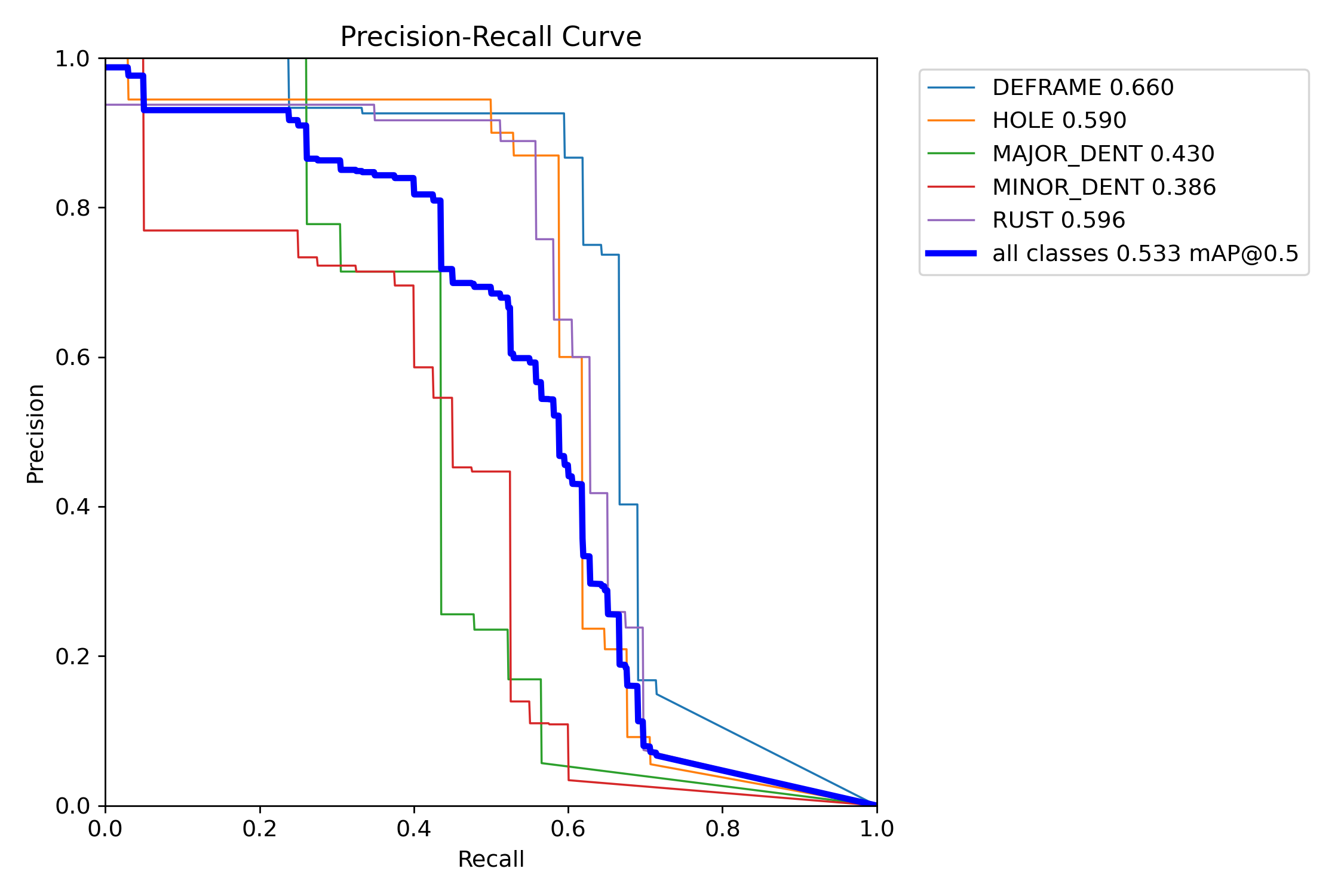
Figure 4: Precision-recall metrics for the GCM-DET model.

Based on the Figure-4, it can be observed that there are significant differences in the detection performance of different defect categories: the average precision (mAP@0.5) of DEFRAME, RUST and HOLE is relatively high, indicating that the model has strong robustness in the location and classification of these types of defects; while MAJOR_DENT and MINOR_DENT are relatively weak, and the accuracy of the curve in the medium and high recall range is significantly reduced, indicating that it is more susceptible to noise interference or feature confusion. Overall, the model achieved an average mAP level of 0.533 in the multi-category defect detection task, indicating that it has a certain detection capability under the condition of IoU=0.5, but there is still room for further improvement of precision and recall, especially in terms of sample size and annotation quality, which may need to be strengthened to improve the detection performance of easily confused or few sample categories.

Table 2: Detection Results of Different Models in NEU-DET

Method	AP@0.5						mAP@0.5	mAP@0.5:0.95	Params(M)	GFLOPs	Size(Mb)
	Cr.	In.	Pa.	Ps.	Rs.	Sc.
RCNN-ResNet50	0.462	0.838	0.895	0.875	0.558	0.905	0.756	-	41.37	13.40	-
RCNN-ResNet101	0.586	0.875	0.879	0.895	0.603	0.936	0.796	-	60.37	18.20	-
DF-DERT	0.440	0.814	0.933	0.875	0.701	0.947	0.785	-	41.00	13.60	-
Focus-DERT	0.553	0.849	0.942	0.826	0.634	0.957	0.793	-	49.20	11.30	-
ES-Net	0.560	0.876	0.883	0.874	0.604	0.949	0.791	-	147.98	-	-
DEA	0.609	0.825	0.943	0.958	0.672	0.741	0.791	-	42.20	-	-
YOLOv5n	0.494	0.852	0.920	0.830	0.607	0.907	0.768	0.456	2.50	7.10	5.03
YOLOv5s	0.527	0.806	0.888	0.861	0.616	0.939	0.773	0.452	9.11	23.80	17.60
YOLOv6n	0.437	0.846	0.926	0.847	0.631	0.925	0.769	0.459	4.23	11.80	8.30
YOLOv6s	0.507	0.852	0.888	0.830	0.653	0.896	0.771	0.439	16.30	44.00	31.30
YOLOv7n-tiny	0.451	0.798	0.904	0.869	0.616	0.827	0.744	0.379	6.02	13.10	11.70
YOLOv8n	0.473	0.843	0.923	0.823	0.624	0.926	0.769	0.444	3.01	8.10	5.97
YOLOv8s	0.508	0.840	0.908	0.847	0.619	0.926	0.775	0.454	11.10	28.40	21.40
LiFSO-Net	0.481	0.864	0.942	0.880	0.644	0.942	0.792	0.479	1.77	5.70	3.69
RDD-YOLO	0.529	0.859	0.944	0.862	0.707	0.966	0.811	-	-	-	-
MD-YOLO	0.467	0.814	0.913	0.851	0.726	0.920	0.782	-	9.00	14.10	-
GCM-DET(Ours)	0.619	0.727	0.980	0.996	0.536	0.979	0.835	0.496	21.80	49.70	83.90

Figure-5 demonstrates the prediction result.

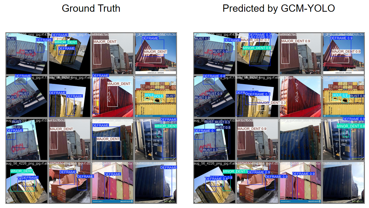
Figure 5: The predicted results of GCM-DET model in CD5-DET vs the ground truth.

4.5 Generalization Study

Generalization experiments are conducted based on the NEU-DET dataset and the performance of GCM-DET with multiple detection models, as shown in Table-2. By comparing classic detection models including YOLOs, U-Net and RCNN models, as well as some improved models such as LiFSO-Net and RDD-YOLO. It is aimed to evaluate the performance of the models in industrial detection tasks.

From the perspective of mAP@0.5, GCM-DET performs significantly better than other models, reaching 0.835, surpassing the closest RDD-YOLO (0.811) and RCNN-ResNet101 (0.796). Compared with the lightweight model, GCM-DET has a significant improvement in mAP@0.5. Especially compared with YOLOv5n (0.768) and YOLOv8n (0.769), the accuracy of GCM-DET has increased by 6.7% and 6.6% respectively. . For the mAP@0.5:0.95 indicator, GCM-DET also showed a significant advantage, reaching 0.473, ahead of most other models, slightly inferior to LiFSO-Net (0.479), but beating YOLOv8n (0.444). This result further proves that GCM-DET can maintain good detection performance under different thresholds and has better generalization ability.

In addition to the improvement in detection accuracy, GCM-DET also performs well in various categories. Among the 6 categories, the individual APs of 4 categories surpassed other models and reached the SOTA indicator. This shows that proposed model has extremely high accuracy in both target classification and localization. In addition, GCM-DET reached nearly over 98% on Pa., Ps. and Sc., achieving almost perfect detection, further verifying the robustness of the model in complex detection tasks.

4.6 Ablation Study

In the ablation experiments, baseline model YOLOv8n is compared marked as S.N.1 in Table-3,4,5. And its different improved versions (M-DET, G-DET, GC-DET and GCM-DET) in three datasets (CD5-DET, NEU-DET and GC10- DET).

Table 3: Ablation Experiments Performed on CD5-DET.

S.N.	Method			Metric
	Gamma	Carafe	SSM	mAP@0.5	mAP@0.5:0.95	Precision	Recall
1				0.257	0.132	0.378	0.288
2			$\surd$	0.447	0.243	0.622	0.458
3	$\surd$			0.463	0.237	0.624	0.503
4	$\surd$	$\surd$		0.509	0.318	0.709	0.510
Ours	$\surd$	$\surd$	$\surd$	0.533	0.374	0.522	0.754

Table 4: Ablation Experiments Performed on NEU-DET.

S.N.	Method			Metric
	Gamma	Carafe	SSM	mAP@0.5	mAP@0.5:0.95	Precision	Recall
1				0.769	0.444	0.666	0.720
2			$\surd$	0.817	0.465	0.771	0.754
3	$\surd$			0.784	0.449	0.673	0.785
4	$\surd$	$\surd$		0.806	0.438	0.734	0.762
Ours	$\surd$	$\surd$	$\surd$	0.835	0.473	0.751	0.763

Table 5: Ablation Experiments Performed on GC10-DET.

S.N.	Method			Metric
	Gamma	Carafe	SSM	mAP@0.5	mAP@0.5:0.95	Precision	Recall
1				0.639	0.320	0.632	0.634
2			$\surd$	0.657	0.320	0.657	0.626
3	$\surd$			0.646	0.326	0.677	0.624
4	$\surd$	$\surd$		0.645	0.325	0.670	0.612
Ours	$\surd$	$\surd$	$\surd$	0.665	0.326	0.681	0.636

1) Remove the SSM module and verify whether the state-space search method is effective. Comparing the baseline model (S.N.1) and SSM (S.N.2) models in Table-3, Table-4 and Table-5, SSM achieved a 19.0% performance improvement in the CD5-DET dataset, a 4.8% performance improvement in NEU-DET, and a 1.8% improvement in GC10-DET on the mAP@0.5 indicator. This shows that the SSM-based architecture can better capture deep content.

2) Remove the dynamic gamma module and verify whether the gamma coefficient correction improves the indicators. The baseline model and the Gamma (S.N.3) model have improved performance in all three datasets, indicating that the dynamically changing Gamma coefficient can repair the grayscale features of the model. Then, the experiment shows that the Carafe (S.N.3) model can obtain more upsampling features compared with the Gamma-Carafe (S.N.4) module with grayscale correction added.

3) Verify whether the fusion model is effective. By merging the backbone network of the SSM architecture and the Gamma-Carafe coefficient, proposed model achieved all-round performance improvement. The innovative fusion strategy of GCM-DET achieved the best mAP@0.5 and mAP@0.5:0.95 on all datasets, demonstrating its excellent ability in multi-scale feature extraction and grayscale feature enhancement. In particular, it achieved a balance between precision and recall, indicating that GCM-DET has better versatility and robustness in practical detection applications.

4.7 Sensitivity analysis of SSMs

Table-6 shows the specific parameters of Mamba models.

Table 6: Window size for different parameters.

model	parameter
	depth	width	max channels
YOLO-Mamba-T	0.33	0.25	1024
YOLO-Mamba-B	0.33	0.5	1024
YOLO-Mamba-L	0.67	0.75	768

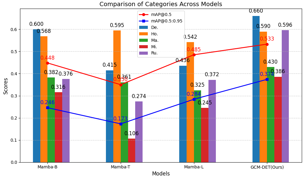
Figure 6: The impact of different window sizes on SSMs performance. Proposed model acheves best in each classes.

The results in the Figure-6 show that Mamba models of different sizes have different sensitivities to different features. For the container damage detection task, Mamba-B is the best window size.

4.8 Discussion

Through comparison of comparative experiments, generalization experiments and ablation experiments, the following are the findings and discussions achieved:

1) Detection performance advantages. GCM-DET shows significant advantages in detection performance, especially in the mAP@0.5 and mAP@0.5:0.95 indicators, which is significantly improved compared to lightweight models such as YOLOv5n and YOLOv6n. This performance improvement is mainly attributed to the introduction of multi-scale feature fusion with adaptive gamma correction and the Mamba mechanism. These innovative designs effectively enhance the feature extraction capabilities of the model and improve the accuracy of target detection.

2) Balance of performance. Compared with more complex models such as MD-YOLO and RDD-YOLO, GCM-DET performs more balanced on the NEU-DET dataset. The combination of adaptive Gamma correction and multi-scale feature fusion enables the model to better adapt to diverse detection tasks. At the same time, the dynamic space search mechanism further optimizes the model’s ability to capture deep features, thereby achieving the best balance between performance and complexity.

In Figure-7, the size of the bubble represents Parameter (M), the x-axis represents GFLOPs, and the y-axis represents mAP@0.5. The closer the model is to the upper left corner, the better the model is. Proposed GCM-DET model effectively balances the amount of computation and accuracy.

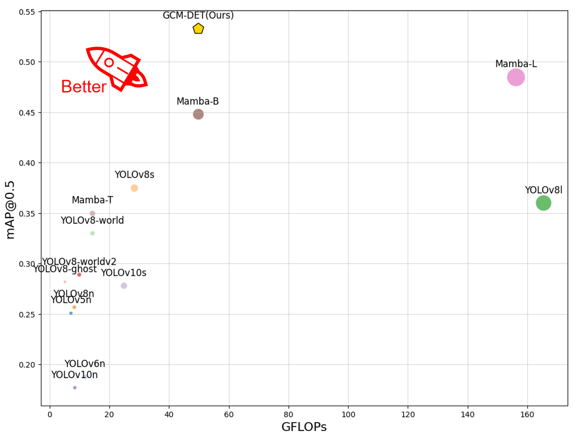
Figure 7: Precision-GFLOPs Trade-off. In the figure, the size of the model points represents the number of parameters. The larger the number of parameters of the model, the more complex the calculation. Proposed model is similar to MAMBA-T in terms of calculation amount, but it effectively improves the detection accuracy.

3) However, the high performance of GCM-DET is accompanied by greater model complexity. Its parameter volume reaches 21.8M, which is significantly higher than other models, such as YOLOv8n (3.0M) and YOLOv5n (2.5M). In terms of GFLOPs, GCM-DET is 49.7, little higher than other models, by contrast to YOLOv5n (7.1 GFLOPs) and YOLOv8n (8.1 GFLOPs). The model size is also large, GCM-DET is 83.9MB, while YOLOv8n and YOLOv5n are only 5.97MB and 5.03MB. Although GCM-DET has increased in computational complexity, the original design of the model is intended for use in task scenarios with extremely high requirements for accuracy. Improvements in detection accuracy can significantly improve system reliability and security, far exceeding the limitations of computing resources. High-precision detection can reduce false positives and false negatives, thereby reducing the error rate of downstream tasks. Especially in automated decision-making systems, a higher mAP@0.5:0.95 means more accurate target location and classification, which greatly improves system reliability and performance.

5 Conclusion

Overall, GCM-DET significantly improves detection accuracy through innovative module design and effective feature fusion strategy, especially showing excellent performance in complex scenes and multi-scale target detection tasks. Experimental results show that GCM-DET reaches the highest mAP@0.5 of 0.533 on the benckmark CD5-DET dataset, verifying its advantages in capturing deep features and enhancing grayscale information. Despite its high computational complexity, GCM-DET provides a reliable and efficient solution for detection tasks requiring high accuracy. Future research will focus on further optimizing the efficiency and adaptability of the model in order to reduce computational costs while maintaining accuracy and meet the needs of more practical applications. In addition, proposed work also plan to expand the dataset to cover more types of targets and scenarios, especially in the field of container defect detection, providing multi-category container defect data to provide broader data support for model performance improvement. This will lay the foundation for a more versatile and efficient defect detection system.

Appendix

5.1 Container Damage Detection Dataset

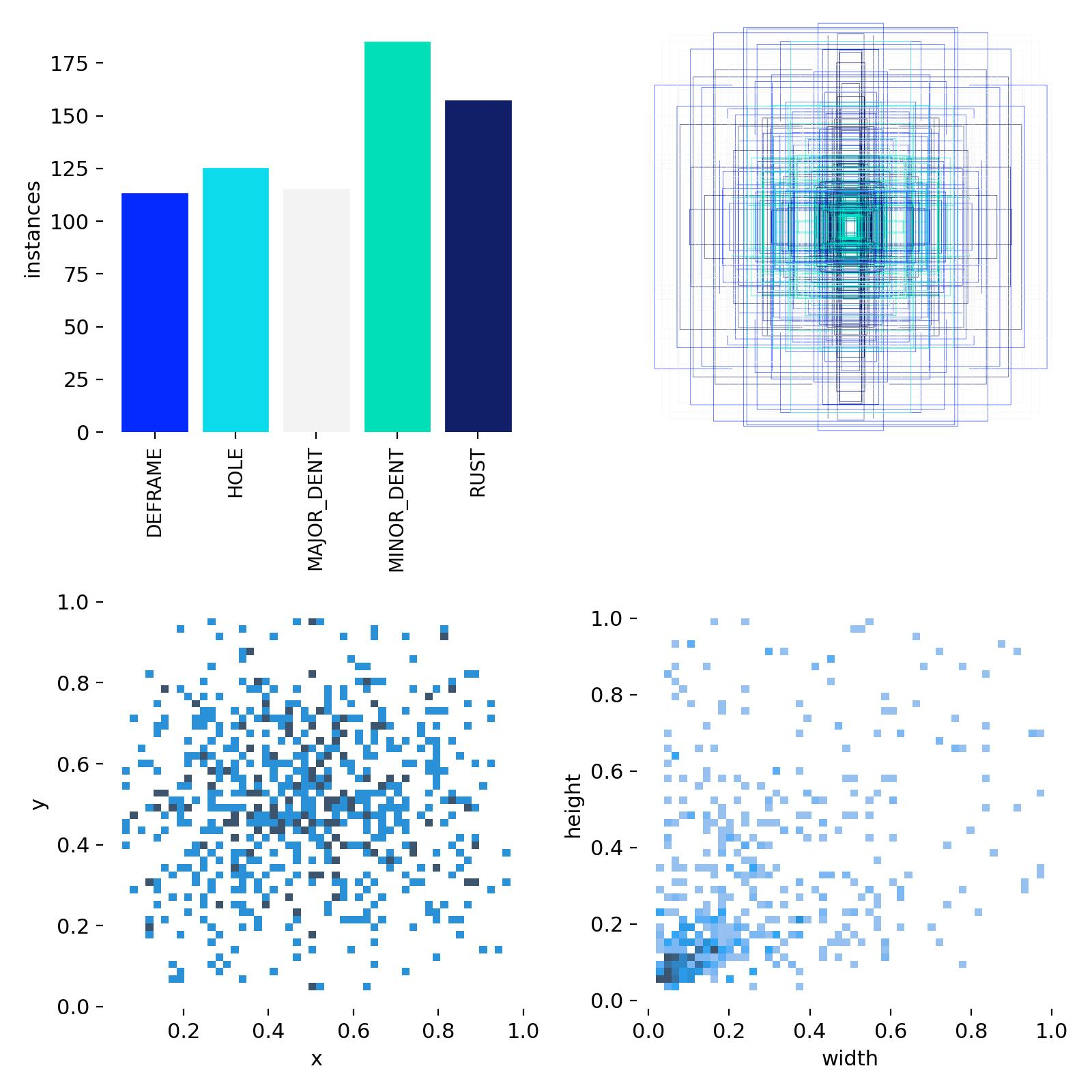
Figure 8: Label and bounding box distribution.

This image dataset is specifically designed for the detection of container appearance damage and comprises five damage categories. The principal characteristics and salient features are as follows:

Categories

1. DEFRAME: Structural deformation or damage to the container frame.

2. HOLE: The presence of a hole in the container.

3. MAJOR_DENT: A relatively severe and extensive dent.

4. MINOR_DENT: A smaller, less severe dent.

5. RUST: Visible traces of rust or corrosion.

Category Distribution

As illustrated by the bar chart, MINOR_DENT exhibits the highest frequency of instances (approximately 180), while DEFRAME and MAJOR_DENT comprises fewer instances (approximately 115). The remaining two categories (HOLE, RUST) consist with 125 and 160 instances.

Bounding-Box Superimposition

The superimposed bounding boxes reveal substantial variations in both position and size, indicating that different types of damage can manifest in multiple regions of the container. Further, the bounding box dimensions (i.e., width and height) span a relatively broad range.

Scatter Plot of Annotation Locations

The lower-left scatter plot represents the relative positioning (x, y) of bounding boxes within the images. Although damage is observed across all regions, the data indicate a higher concentration around the central area (approximately 0.3–0.7 in both x and y coordinates) as well as some instances near the periphery.

Scatter Plot of Bounding Box Sizes

The lower-right scatter plot illustrates bounding box dimensions, measured by width and height. A majority of these bounding boxes are relatively small in size (both width and height below 0.2), though larger damaged regions are also present.

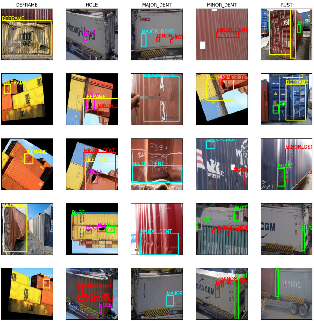
Figure 9: Example images of CD5-DET.

An image contains multiple categories. Figure-9 shows the details of the image.

GCM-DET can give target boxes and labels close to the ground truth for container defects in most samples, with high confidence. However, some samples also have problems such as missed detection (such as no box or missing category) and wrong detection (such as deviation in category judgment or multiple boxes). In particular, defect types with similar appearance features or unclear edge contours (MAJOR_DENT and MINOR_DENT) are more likely to be confused. At the same time, the color of the container body and the defective area are prone to local occlusion or light reflection, which may cause the model to recognize blurred boundaries or low confidence. These phenomena show that for defects with similar features, small areas or irregular shapes, more high-quality training data and better feature extraction methods are still needed to further improve the accuracy and robustness of detection.

References

- [1] Juan Terven, Diana-Margarita Córdova-Esparza, and Julio-Alejandro Romero-González. A comprehensive review of yolo architectures in computer vision: From yolov1 to yolov8 and yolo-nas. Machine Learning and Knowledge Extraction, 5(4):1680–1716, 2023.
- [2] Jiaqi Wang, Kai Chen, Rui Xu, Ziwei Liu, Chen Change Loy, and Dahua Lin. Carafe: Content-aware reassembly of features. In Proceedings of the IEEE/CVF International Conference on Computer Vision (ICCV), October 2019.
- [3] Lianghui Zhu, Bencheng Liao, Qian Zhang, Xinlong Wang, Wenyu Liu, and Xinggang Wang. Vision mamba: Efficient visual representation learning with bidirectional state space model. arXiv preprint arXiv:2401.09417, 2024.
- [4] Yi-Fan Zhang, Weiqiang Ren, Zhang Zhang, Zhen Jia, Liang Wang, and Tieniu Tan. Focal and efficient iou loss for accurate bounding box regression. Neurocomputing, 506:146–157, 2022.
- [5] Kechen Song and Yunhui Yan. A noise robust method based on completed local binary patterns for hot-rolled steel strip surface defects. Applied Surface Science, 285:858–864, 2013.
- [6] Xiaoming Lv, Fajie Duan, Jia-jia Jiang, Xiao Fu, and Lin Gan. Deep metallic surface defect detection: The new benchmark and detection network. Sensors, 20(6):1562, 2020.
- [7] Shuzong Chen, Shengquan Jiang, Xiaoyu Wang, Pu Sun, Changchun Hua, and Jie Sun. An efficient detector for detecting surface defects on cold-rolled steel strips. Engineering Applications of Artificial Intelligence, 138:109325, 2024.
- [8] Sijin Sun, Ming Deng, Jiawei Luo, Xiaohang Zheng, and Yang Pan. St-yolo: An improved metal defect detection model based on yolov5. In Proceedings of the 2024 3rd Asia Conference on Algorithms, Computing and Machine Learning, pages 158–164, 2024.
- [9] Xiaoyu Wang, Tony X Han, and Shuicheng Yan. An hog-lbp human detector with partial occlusion handling. In 2009 IEEE 12th international conference on computer vision, pages 32–39. IEEE, 2009.
- [10] Jianguo Li and Yimin Zhang. Learning surf cascade for fast and accurate object detection. In Proceedings of the IEEE conference on computer vision and pattern recognition, pages 3468–3475, 2013.
- [11] Phillip Ian Wilson and John Fernandez. Facial feature detection using haar classifiers. Journal of computing sciences in colleges, 21(4):127–133, 2006.
- [12] Ross Girshick, Jeff Donahue, Trevor Darrell, and Jitendra Malik. Rich feature hierarchies for accurate object detection and semantic segmentation. In Proceedings of the IEEE conference on computer vision and pattern recognition, pages 580–587, 2014.
- [13] Shaoqing Ren. Faster r-cnn: Towards real-time object detection with region proposal networks. arXiv preprint arXiv:1506.01497, 2015.
- [14] Kaiming He, Georgia Gkioxari, Piotr Dollár, and Ross Girshick. Mask r-cnn. In Proceedings of the IEEE international conference on computer vision, pages 2961–2969, 2017.
- [15] Muhammad Hussain. Yolo-v1 to yolo-v8, the rise of yolo and its complementary nature toward digital manufacturing and industrial defect detection. Machines, 11(7), 2023.
- [16] Sanghyun Woo, Jongchan Park, Joon-Young Lee, and In So Kweon. Cbam: Convolutional block attention module. In Proceedings of the European conference on computer vision (ECCV), pages 3–19, 2018.
- [17] Tianyong Wu and Youkou Dong. Yolo-se: Improved yolov8 for remote sensing object detection and recognition. Applied Sciences, 13(24):12977, 2023.
- [18] Zixiao Zhang, Xiaoqiang Lu, Guojin Cao, Yuting Yang, Licheng Jiao, and Fang Liu. Vit-yolo: Transformer-based yolo for object detection. In Proceedings of the IEEE/CVF international conference on computer vision, pages 2799–2808, 2021.
- [19] Xiangyu Zhang, Xinyu Zhou, Mengxiao Lin, and Jian Sun. Shufflenet: An extremely efficient convolutional neural network for mobile devices. In Proceedings of the IEEE conference on computer vision and pattern recognition, pages 6848–6856, 2018.
- [20] Andrew G Howard. Mobilenets: Efficient convolutional neural networks for mobile vision applications. arXiv preprint arXiv:1704.04861, 2017.
- [21] Shuo Zhang, Shengbing Che, Zhen Liu, and Xu Zhang. A real-time and lightweight traffic sign detection method based on ghost-yolo. Multimedia Tools and Applications, 82(17):26063–26087, 2023.
- [22] Glenn Jocher, Jing Qiu, and Ayush Chaurasia. Ultralytics YOLO, January 2023.
- [23] Albert Gu, Karan Goel, and Christopher R’e. Efficiently modeling long sequences with structured state spaces. ArXiv, abs/2111.00396, 2021.
- [24] Albert Gu and Tri Dao. Mamba: Linear-time sequence modeling with selective state spaces. ArXiv, abs/2312.00752, 2023.
- [25] Zeyu Wang, Chen Li, Huiying Xu, and Xinzhong Zhu. Mamba yolo: Ssms-based yolo for object detection. ArXiv, abs/2406.05835, 2024.
- [26] Yuming Chen, Xinbin Yuan, Ruiqi Wu, Jiabao Wang, Qibin Hou, and Mingg-Ming Cheng. Yolo-ms: Rethinking multi-scale representation learning for real-time object detection. ArXiv, abs/2308.05480, 2023.
- [27] Alexey Dosovitskiy, Lucas Beyer, Alexander Kolesnikov, Dirk Weissenborn, Xiaohua Zhai, Thomas Unterthiner, Mostafa Dehghani, Matthias Minderer, Georg Heigold, Sylvain Gelly, Jakob Uszkoreit, and Neil Houlsby. An image is worth 16x16 words: Transformers for image recognition at scale. ArXiv, abs/2010.11929, 2020.
- [28] Yue Liu, Yunjie Tian, Yuzhong Zhao, Hongtian Yu, Lingxi Xie, Yaowei Wang, Qixiang Ye, and Yunfan Liu. Vmamba: Visual state space model. ArXiv, abs/2401.10166, 2024.