ACCORD: Alleviating Concept Coupling through Dependence Regularization for Text-to-Image Diffusion Personalization

Abstract

Image personalization has garnered attention for its ability to customize Text-to-Image generation using only a few reference images. However, a key challenge in image personalization is the issue of conceptual coupling, where the limited number of reference images leads the model to form unwanted associations between the personalization target and other concepts. Current methods attempt to tackle this issue indirectly, leading to a suboptimal balance between text control and personalization fidelity. In this paper, we take a direct approach to the concept coupling problem through statistical analysis, revealing that it stems from two distinct sources of dependence discrepancies. We therefore propose two complementary plug-and-play loss functions: Denoising Decouple Loss and Prior Decouple loss, each designed to minimize one type of dependence discrepancy. Extensive experiments demonstrate that our approach achieves a superior trade-off between text control and personalization fidelity.

1 Introduction

The advancement of Text-to-Image (T2I) Diffusion Models [1, 2] has lowered the barrier to generating high-quality and imaginative images from text prompts. However, pretrained T2I models often struggle to accurately produce personalized images, such as those depicting private pets or unique artistic styles. As a result, personalized image generation has recently gained significant attention, necessitating users to provide several reference images pertaining to the personalization target, which enables T2I models to create images of the personalization target based on text prompts.

The primary challenge of image personalization is “concept coupling”. Due to the limited availability of reference images for the personaliztion target, the model tends to confuse the target with other concepts that appear alongside it in these images. This entanglement hinders the model’s ability to accurately control the attributes associated with the personalization target based on text. For example, as shown in Fig. 1, the model may interpret "a person carrying a backpack" as the primary focus, rather than "backpack," because these elements frequently co-occur in the reference images. Consequently, the generated images often deviate from the intended text prompts, frequently including an unintended person in the output.

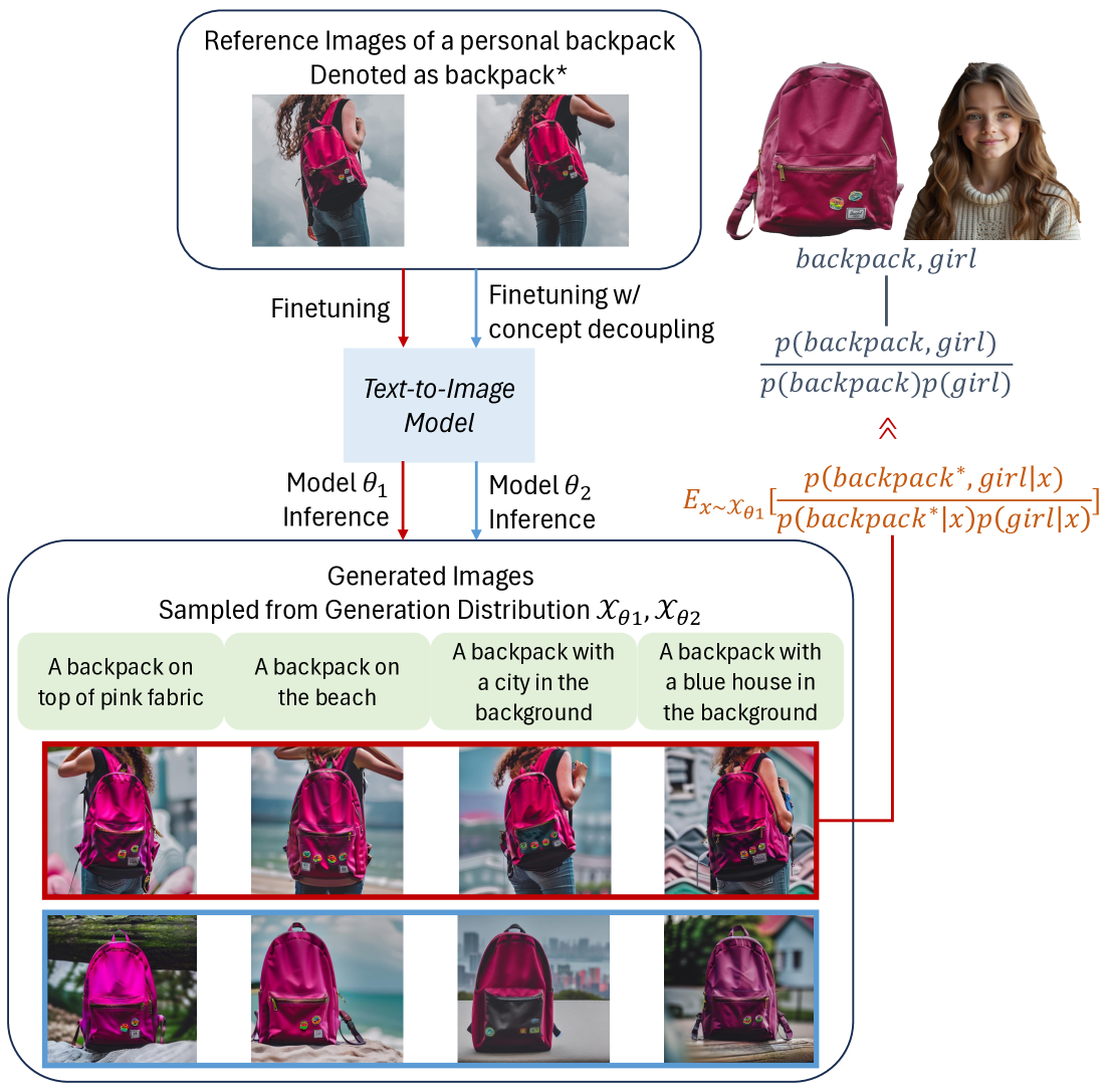
Figure 1: Illustration of the concept coupling problem. The personalization target is a “backpack”, but in the reference images, the backpack and a girl always appear together. This causes the model finetuned without concept decoupling to frequently generate an additional girl and not fully adhere to the prompt. Statistically, the co-occurrence of “backpack” and “girl” in generated images is significantly higher than the inherent concept dependence.

However, existing image personalization methods fail to directly address the issue of concept coupling. The current methods for mitigating concept coupling can be broadly categorized into three types: data regularization, weight regularization, and loss regularization. Data regularization methods [3, 4], generate or retrieve a regularization dataset based on the superclass of the personalization target to preserve the model’s prior knowledge during training. Nevertheless, the limited size of the regularization dataset cannot ensure that inter-concept relationships align with their inherent relationships, and simultaneous training on regularization and reference images often compromises personalization fidelity. Weight regularization approaches, like SVDiff [5] and OFT [6], mitigate the risk of overfitting to reference images by constraining the optimization space of parameters, such as by fine-tuning only the cross-attention layer parameters. Such constraints do not guarantee selective learning of the personalization target and other concepts, and the personalization fidelity may degrade as parameters are constrained. Loss regularization methods [7, 8] introduce auxiliary loss functions for regularization, but existing methods rely on empirical choices for optimization objectives and lack theoretical guarantees for reducing concept coupling.

In this paper, we directly frame concept coupling as a statistical problem, where personalized Text-to-Image (T2I) models create unintended dependencies between the personalization target and other concepts in reference images. As illustrated in Fig. 1, when personalizing for concepts like ’backpack’ alongside ’girl’, the model learns artificially strong associations that exceed their natural relationship in the training data. We analyze this concept coupling by breaking it down into two components: the Denoising Dependence Discrepancy and the Prior Dependence Discrepancy. To minimize these discrepancies, we propose ACCORD, a plug-and-play method that employs two specialized loss functions for dependence regularization.

Specifically, we propose the Denoising Decouple Loss (DDLoss) and the Prior Decouple Loss (PDLoss) to reduce the denoising dependence discrepancy and prior dependence discrepancy, respectively. This enables ACCORD to eliminate the need for regularization datasets and excessive weight regularization as in previous works; instead, it directly minimizes over-dependencies between concepts. The DDLoss functions by establishing an upper bound on the denoising dependence discrepancy, aggregating the discrepancies between consecutive denoising steps and utilizing the diffusion model as an implicit classifier to minimize these step-wise differences. Complementing this, the PDLoss addresses cases where training the personalization target’s representation [9, 10] increases the prior dependence discrepancy, using CLIP’s [11] conditional classification capabilities to minimize this effect. Experiments demonstrate that the proposed loss functions alleviate the concept coupling issue in image personalization more effectively, achieving a better balance between text control and personalization fidelity. Our contributions can be summarized as follows:

• We formally characterize concept coupling in image personalization as a statistical problem of unintended dependencies and propose ACCORD, a plug-and-play method that directly addresses concept coupling without requiring regularization datasets or extensive weight constraints.

• We identify two distinct sources of dependence discrepancies in concept coupling: Denoising Dependence Discrepancy and Prior Dependence Discrepancy. To address these discrepancies, we propose Denoising Decouple Loss and Prior Decouple Loss, respectively.

• Experimental results demonstrate the superiority of ACCORD in image personalization. Moreover, the proposed losses prove effective in zero-shot conditional control tasks, highlighting the potential of concept decoupling.

2 Related Works

Test Time Finetuning-based Image Personalization. Test-time fine-tuning methods personalize pre-trained T2I models by adapting them to reference images of the personalization target. Although this approach requires time and computational resources for training, it achieves greater flexibility for diverse personalization demands and often strikes a better balance between text control and personalization fidelity. Therefore, this paper focuses on improving the test-time fine-tuning method.

In terms of addressing the concept coupling problem, test-time fine-tuning methods can be broadly categorized into three types: data regularization, weight regularization, and loss regularization. In data regularization methods, Dreambooth [3] mitigates overfitting by using a pretrained T2I model to generate a set of images for the superclass of the personalization target and trains on both reference and regularization images. Custom Diffusion [4] enhances the quality of regularization images by retrieving them from real images. Specialist Diffusion [12] designs extensive data augmentation techniques. However, the limited size of the regularization dataset hampers its ability to accurately capture the inherent relationships among concepts, misaligning the optimization objective with reducing concept coupling. Furthermore, simultaneous training on regularization and reference images often impairs personalization fidelity due to their substantial appearance differences. Weight regularization methods [9, 13, 5, 6] finetune the parameters of the T2I model in a constrained manner, such as by adjusting only the text embedding of the personalization target or the singular values of the weight matrices. While these methods mitigate overfitting to reference images, they lack a tailored mechanism to distinguish between the personalization target and other concepts, potentially reducing personalization fidelity by constraining the parameter space. Loss regularization methods include Specialist Diffusion [12], MagiCapture [14], Facechain-SuDe [7], , among others. Specialist Diffusion designs a content loss that aims to maximize the similarity between generated and reference images in the CLIP image space. MagiCapture employs masked reconstruction based on facial masks to disentangle face and style learning. Facechain-SuDe applies concepts from object-oriented programming to enhance the likelihood that a generated image, conditioned on the personalization target, is correctly classified under its superclass. However, these loss functions rely on empirically selected optimization objectives and may not fully align with concept decoupling.

In contrast to previous works that indirectly reduce concept coupling, this paper reformulates concept coupling as a problem of excessive dependency between two concepts and derives two dependency-regularization-based loss functions to directly minimize this coupling.

Zero-shot Image Personalization. Unlike test-time finetuning methods, zero-shot image personalization methods reduce the need for test-time training but require substantial amounts of data for pretraining. Models developed using these methods are generally limited to specific image domains, such as faces and objects, which restricts their capacity to meet diverse personalization demands. We introduce representative methods below.

For subject personalization, InstantBooth [15] employs a visual encoder to capture both coarse and fine image features from reference images. BLIP-Diffusion [16] fine-tunes BLIP-2 [17] as a subject representation extractor for obtaining multimodal representations. ELITE [18] develops a global and a local mapping network to encode the visual concepts of reference images into hierarchical textual words. In contrast to these methods, [8] addresses the challenge of weak text control by removing the projection of visual embeddings onto text embeddings. For facial personalization, InstantID [19] crops facial regions from reference images to extract appearance and structural features. For style personalization, InstantStyle [20] identifies the style-controlling layers in SDXL [21] and achieves style transfer by feeding IP-Adapter [10] features into these weights.

This paper devotes less focus to zero-shot image personalization methods. Nevertheless, our experiments also reveal the potential of the proposed losses for these methods.

3 Method

3.1 Text-to-Image (T2I) Diffusion Models

We begin with a brief introduction to the T2I Diffusion Model [1], which establishes a mapping between the image distribution and the standard Gaussian distribution via a forward noise-adding process and a reverse denoising process. Specifically, the forward process is composed of $T$ steps, gradually introducing Gaussian noise into a clear image or its latent code ${\mathbf{x}}_{0}$. The noisy code at time step $t\in\{1,2,...,T\}$ is calculated as follows:

$${\mathbf{x}}_{t}=\sqrt{\alpha_{t}}{\mathbf{x}}_{0}+\sqrt{1-\alpha_{t}}\bm{\epsilon},$$ (1)

where $\bm{\epsilon}\sim{\mathcal{N}}(\mathbf{0},{\bm{I}})$ represents Gaussian noise, and $\alpha_{t}$ modulates the retention of the original image, decreasing as $t$ increases. When $T$ is sufficiently large, ${\mathbf{x}}_{T}$ approximately follows a multivariate standard Gaussian distribution.

The reverse process is modeled as a Markov chain, where a network ${\mathcal{U}}_{\theta}$ with parameters $\theta$ is used to estimate the parameters of the true posterior distribution $q({\mathbf{x}}_{t-1}|{\mathbf{x}}_{t},{\mathbf{x}}_{0})$ based on $t$ and ${\mathbf{x}}_{t}$, thereby achieving denoising of the noisy code. The optimization objective can be expressed as:

$$\mathbb{E}_{{\mathbf{x}}_{0},\bm{\epsilon},{\mathbf{c}},t}[\frac{1}{2\bm{\sigma}_{t}^{2}}\|{\mathbf{x}}_{t-1}-{\mathcal{U}}_{\theta}({\mathbf{x}}_{t},{\mathbf{c}},t)\|^{2}].$$ (2)

Where $\bm{\sigma}_{t}$ represents the standard deviation of the noisy code at time step $t$, and ${\mathcal{U}}_{\theta}({\mathbf{x}}_{t},{\mathbf{c}},t)$ is the output of the denoising model. During inference, the noisy code ${\mathbf{x}}_{t-1}$ at time step $t-1$ can be sampled from ${\mathcal{N}}({\mathcal{U}}_{\theta}({\mathbf{x}}_{t},{\mathbf{c}},t),\bm{\sigma}_{t}^{2}{\bm{I}})$, yielding ${\mathbf{x}}_{t-1}={\mathcal{U}}_{\theta}({\mathbf{x}}_{t},{\mathbf{c}},t)+\bm{\sigma}_{t}\bm{\epsilon}_{t}$, where $\bm{\epsilon}\sim{\mathcal{N}}(\mathbf{0},{\bm{I}})$. Note that the text representation or the conditioning information ${\mathbf{c}}$ is also fed into the denoising model to control the generation.

To facilitate the subsequent discussions, we further introduce the conditional dependence coefficient $r$ for two concepts ${\mathbf{c}}_{p}$ and ${\mathbf{c}}_{g}$, present in the generated image or its latent code based on $({\mathbf{c}}_{p},{\mathbf{c}}_{g})$ at time step $t$, i.e., ${\mathbf{x}}_{\theta,t}:={\mathcal{U}}_{\theta}\big{(}{\mathbf{x}}_{t+1},({\mathbf{c}}_{p},{\mathbf{c}}_{g}),t+1\big{)}$. This coefficient can be defined as the ratio between the joint probability of the two concepts occurring together in ${\mathbf{x}}_{\theta,t}$ and the probability of their independent occurrences in the same representation:

$$r({\mathbf{c}}_{p},{\mathbf{c}}_{g}|{\mathbf{x}}_{\theta,t})=\frac{p({\mathbf{c}}_{p},{\mathbf{c}}_{g}|{\mathbf{x}}_{\theta,t})}{p({\mathbf{c}}_{p}|{\mathbf{x}}_{\theta,t})p({\mathbf{c}}_{g}|{\mathbf{x}}_{\theta,t})}.$$ (3)

According to probability theory, ${\mathbf{c}}_{p}$ and ${\mathbf{c}}_{g}$ are conditionally independent given ${\mathbf{x}}_{\theta,t}$ when $r({\mathbf{c}}_{p},{\mathbf{c}}_{g}|{\mathbf{x}}_{\theta,t})=1$; they are conditionally dependent otherwise.

We provide a summary of all notations in Appendix Tab. 5.

3.2 Concept Coupling in Image Personalization

Test-time finetuning methods are designed to achieve image personalization by fine-tuning a pretrained T2I model on a limited set of reference images with the personalization target, denoted as ${\mathbb{D}}=\{({\mathbf{x}}^{i},{\mathbf{c}}^{i})\}_{i=1}^{N}$. Here, $N$ is the number of training samples, typically ranging from 3 to 6. ${\mathbf{x}}^{i}$ and ${\mathbf{c}}^{i}$ represent the reference image and the correponding generation condition for the $i$-th pair, respectively. Note that ${\mathbf{c}}^{i}$ can be either an image caption or a combination of the caption and visual features extracted from the reference images for personalization purposes. In instances where captions for ${\mathbf{x}}^{i}$ are absent, we employ Vision Language Models (VLMs) [22] to generate image captions, aligning with practices in the community. This approach, compared to using prompt templates [3], yields more meaningful textual concepts and assists in the decoupling of concepts.

One issue that plagues image personalization is concept coupling. As illustrated in Fig. 1, although the personalization target ${\mathbf{c}}_{p}$ is a specifically designed red backpack, the training set ${\mathbb{D}}$ consistently pairs the personalized backpack ${\mathbf{c}}_{p}$ with a girl ${\mathbf{c}}_{g}$. Consequently, the adapted T2I model often tends to generate an additional girl during inference, which contradicts the original prompt. This phenomenon can be statistically characterized as:

$$\mathbb{E}_{{\mathbf{x}}_{\theta}}[|\log r({\mathbf{c}}_{p},{\mathbf{c}}_{g}|{\mathbf{x}}_{\theta,0})-\log r({\mathbf{c}}_{s},{\mathbf{c}}_{g})|]\gg 0,$$ (4)

where $|\cdot|$ denotes the absolute value, ${\mathbf{x}}_{\theta,0}$ denotes the image generated by the T2I model or its latent code, ${\mathbf{c}}_{p}$ and ${\mathbf{c}}_{g}$ represents the personalized target condition and the general text condition respectively, while ${\mathbf{c}}_{s}$ denotes superclass of ${\mathbf{c}}_{p}$. Additionally, $r({\mathbf{c}}_{s},{\mathbf{c}}_{g})=p({\mathbf{c}}_{s},{\mathbf{c}}_{g})/p({\mathbf{c}}_{s})/p({\mathbf{c}}_{g})$. In this context, ${\mathbf{c}}_{s}$ embodies a general backpack, thus encompassing the overall properties of ${\mathbf{c}}_{p}$ and further characterizing the inherent relationships with other general concepts represented by ${\mathbf{c}}_{g}$ [3, 7]. The essence of the equation above is that the generated images ${\mathbf{x}}_{\theta,0}$ typically introduce additional interdependencies between ${\mathbf{c}}_{p}$ and ${\mathbf{c}}_{g}$ that are not present in the inherent prior relationships between ${\mathbf{c}}_{s}$ and ${\mathbf{c}}_{g}$. Indeed,

Lemma 1.

$\mathbb{E}_{{\mathbf{x}}_{\theta}}[|\log r({\mathbf{c}}_{p},{\mathbf{c}}_{g}|{\mathbf{x}}_{\theta,0})-\log r({\mathbf{c}}_{s},{\mathbf{c}}_{g})|]>0$ holds when either (i) $r({\mathbf{c}}_{p},{\mathbf{c}}_{g}|{\mathbf{x}}_{\theta,0})>r({\mathbf{c}}_{s},{\mathbf{c}}_{g})$ (overly positive dependence) or (ii) $r({\mathbf{c}}_{p},{\mathbf{c}}_{g}|{\mathbf{x}}_{\theta,0})<r({\mathbf{c}}_{s},{\mathbf{c}}_{g})$ (overly negative dependence). The equality is achieved if and only if $r({\mathbf{c}}_{p},{\mathbf{c}}_{g}|{\mathbf{x}}_{\theta,0})=r({\mathbf{c}}_{s},{\mathbf{c}}_{g})$.

Thus, the fundamental goal of concept decoupling is to correct the conditional dependence coefficient between ${\mathbf{c}}_{p}$ and ${\mathbf{c}}_{g}$ in the generated images so that it approximates the prior concept dependence between ${\mathbf{c}}_{s}$ and ${\mathbf{c}}_{g}$.

3.3 Sources of Dependencies in Image Personalization

The direct computation and minimization of the left-hand side (LHS) of Eq. (4) pose significant challenges due to the absence of a closed-form expression. Instead, we identify that it can be decomposed into two computable dependence discrepancies, as shown in Theorem 1.

Theorem 1.

The LHS of Eq. (4) can be decomposed into the following two terms:

$$\mathbb{E}_{{\mathbf{x}}_{\theta}}\Big{[}|\underbrace{\log r({\mathbf{c}}_{p},{\mathbf{c}}_{g}|{\mathbf{x}}_{\theta,0})-\log r({\mathbf{c}}_{p},{\mathbf{c}}_{g}|{\mathbf{x}}_{T})}_{\text{ \leavevmode\hbox to7.49pt{\vbox to7.49pt{\text{[drawing]}}} Denoising Dependence Discrepancy}}+\underbrace{\log r({\mathbf{c}}_{p},{\mathbf{c}}_{g})-\log r({\mathbf{c}}_{s},{\mathbf{c}}_{g})}_{\text{ \leavevmode\hbox to7.49pt{\vbox to7.49pt{\text{[drawing]}}} Prior Dependence Discrepancy}}|\Big{]},$$ (5)

where ${\mathbf{x}}_{T}$ denotes multivariate standard Gaussian noise.

Proof.

Since ${\mathbf{x}}_{T}$ is Gaussian noise sampled independently of the conditions ${\mathbf{c}}_{p}$ and ${\mathbf{c}}_{g}$, we have $p({\mathbf{x}}_{T}|{\mathbf{c}})=p({\mathbf{x}}_{T})$. By applying Bayes’ theorem, we have $p({\mathbf{c}}|{\mathbf{x}}_{T})=p({\mathbf{c}})p({\mathbf{x}}_{T}|{\mathbf{c}})/p({\mathbf{x}}_{T})=p({\mathbf{c}})$. It follows that

$$\log\frac{p({\mathbf{c}}_{p},{\mathbf{c}}_{g}|{\mathbf{x}}_{T})}{p({\mathbf{c}}_{p}|{\mathbf{x}}_{T})p({\mathbf{c}}_{g}|{\mathbf{x}}_{T})}=\log\frac{p({\mathbf{c}}_{p},{\mathbf{c}}_{g})}{p({\mathbf{c}}_{p})p({\mathbf{c}}_{g})},$$ (6)

and so $\log r({\mathbf{c}}_{p},{\mathbf{c}}_{g}|{\mathbf{x}}_{T})=\log r({\mathbf{c}}_{p},{\mathbf{c}}_{g})$. This indicates that the expression in (5) equals the LHS of Eq. (4). ∎

In expression (5), the denoising dependence discrepancy captures the change in conditional dependence between ${\mathbf{c}}_{p}$ and ${\mathbf{c}}_{g}$ introduced during denoising, whereas the prior dependence discrepancy reflects the alteration in prior dependence due to deviations of ${\mathbf{c}}_{p}$ from ${\mathbf{c}}_{s}$. The conditional dependence coefficient of ${\mathbf{c}}_{p}$ and ${\mathbf{c}}_{g}$ on ${\mathbf{x}}_{T}$ in Eq. (6) bridge the denoising dependence and prior dependence.

Building on this decomposition, we propose ACCORD, a plug-and-play method comprising two loss functions: the Denoising Decouple Loss (DDLoss) and the Prior Decouple Loss (PDLoss). The DDLoss minimizes the denoising dependence discrepancy by leveraging the implicit classification capabilities of the diffusion model, while the PDLoss alleviates prior dependence discrepancy, particularly when ${\mathbf{c}}_{p}$ is trainable, by utilizing the classification capability of CLIP. Collectively, these strategies work synergistically to minimize concept coupling, which will be elaborated below.

3.4 Denoising Decouple Loss (DDLoss)

We observe that directly minimizing the denoising dependence discrepancy term in Eq. (5) is not well-aligned with the time step sampling mechanism employed during the training of diffusion models. This incompatibility arises because the term connects the first and last time steps, bypassing the relationships between successive steps. To address this issue, we propose to relax this term by upper-bounding it with the sum of dependence discrepancies between adjacent denoising steps:

$$\,|\log r({\mathbf{c}}_{p},{\mathbf{c}}_{g}|{\mathbf{x}}_{\theta,0})-\log r({\mathbf{c}}_{p},{\mathbf{c}}_{g}|{\mathbf{x}}_{T})|$$

$$= \,|\sum_{t=1}^{T}\log r({\mathbf{c}}_{p},{\mathbf{c}}_{g}|{\mathbf{x}}_{\theta,t-1})-\log r({\mathbf{c}}_{p},{\mathbf{c}}_{g}|{\mathbf{x}}_{\theta,t})|\leq\sum_{t=1}^{T}|\log r({\mathbf{c}}_{p},{\mathbf{c}}_{g}|{\mathbf{x}}_{\theta,t-1})-\log r({\mathbf{c}}_{p},{\mathbf{c}}_{g}|{\mathbf{x}}_{\theta,t})|.$$ (7)

The above relaxation holds due to the triangle inequality.

Next, by exploiting the diffusion model as an implicit classifier [23, 7], we can derive a closed-form expression for $\log r({\mathbf{c}}_{p},{\mathbf{c}}_{g}|{\mathbf{x}}_{\theta,t-1})-\log r({\mathbf{c}}_{p},{\mathbf{c}}_{g}|{\mathbf{x}}_{\theta,t})$:

Theorem 2.

The dependence discrepancy between successive time steps in diffusion models can be computed as:

$$\,\log r({\mathbf{c}}_{p},{\mathbf{c}}_{g}|{\mathbf{x}}_{\theta,t-1})-\log r({\mathbf{c}}_{p},{\mathbf{c}}_{g}|{\mathbf{x}}_{\theta,t})$$

$$= \,\frac{1}{2\bm{\sigma}_{t}^{2}}\Big{[}\|{\mathcal{U}}_{\theta}\big{(}{\mathbf{x}}_{t},({\mathbf{c}}_{p},{\mathbf{c}}_{g}),t\big{)}-{\mathcal{U}}_{\theta}\big{(}{\mathbf{x}}_{\theta,t},{\mathbf{c}}_{p},t\big{)}\|^{2}$$

$$\,+\|{\mathcal{U}}_{\theta}\big{(}{\mathbf{x}}_{t},({\mathbf{c}}_{p},{\mathbf{c}}_{g}),t\big{)}-{\mathcal{U}}_{\theta}\big{(}{\mathbf{x}}_{\theta,t},{\mathbf{c}}_{g},t\big{)}\|^{2}$$

$$\,-\|{\mathcal{U}}_{\theta}\big{(}{\mathbf{x}}_{t},({\mathbf{c}}_{p},{\mathbf{c}}_{g}),t\big{)}-{\mathcal{U}}_{\theta}\big{(}{\mathbf{x}}_{\theta,t},\varnothing,t\big{)}\|^{2}\Big{]},$$ (8)

where $\varnothing$ denotes an empty control condition.

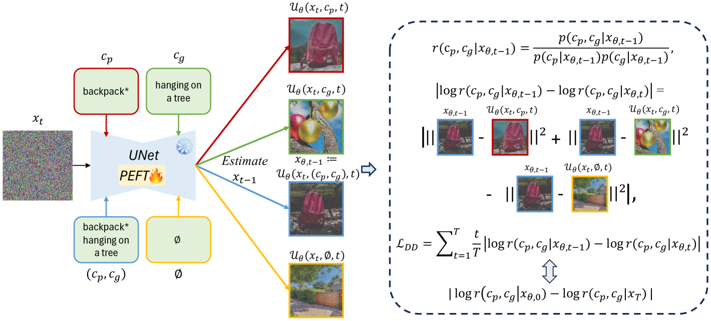
Figure 2: Calculation of the Denoising Decouple Loss $\mathcal{L}_{\text{DD}}$. The UNet estimates ${\mathbf{x}}_{t-1}$ based on ${\mathbf{x}}_{t}$ and four different conditions, then constrains the four denoising results. The objective of $\mathcal{L}_{\text{DD}}$ is to prevent the conditional dependence coefficient between the personalization target ${\mathbf{c}}_{p}$ and general text conditions ${\mathbf{c}}_{g}$ from varying significantly in the denoising results of adjacent timesteps.

Proof.

For arbitrary conditions $\hat{\mathbf{c}}$, we can employ Bayes’ theorem as follows:

$$p(\hat{\mathbf{c}}|{\mathbf{x}}_{\theta,t-1})=\frac{p(\hat{\mathbf{c}}|{\mathbf{x}}_{\theta,t})p({\mathbf{x}}_{\theta,t-1}|{\mathbf{x}}_{\theta,t},\hat{\mathbf{c}})}{p({\mathbf{x}}_{\theta,t-1}|{\mathbf{x}}_{\theta,t})}.$$ (9)

In diffusion models, $p({\mathbf{x}}_{\theta,t-1}|{\mathbf{x}}_{\theta,t},\hat{\mathbf{c}})$ is parameterized as a Gaussian distribution (cf. Section 3.1):

$$p({\mathbf{x}}_{\theta,t-1}|{\mathbf{x}}_{\theta,t},\hat{\mathbf{c}}) ={\mathcal{N}}\big{(}{\mathbf{x}}_{\theta,t-1};{\mathcal{U}}_{\theta}({\mathbf{x}}_{\theta,t},\hat{\mathbf{c}},t),\bm{\sigma}_{t}^{2}{\bm{I}}\big{)},$$ (10)

Note that $\hat{\mathbf{c}}$ is an arbitrary condition that may consider conditions other than $({\mathbf{c}}_{p},{\mathbf{c}}_{g})$. Similarly, $p({\mathbf{x}}_{\theta,t-1}|{\mathbf{x}}_{\theta,t})$ can be derived based on (9) by subsituting $\hat{\mathbf{c}}$ with $\varnothing$. As such, Eq. (9) enables diffusion models to ascertain whether ${\mathbf{x}}_{\theta,t-1}$ belongs to the class defined by $\hat{\mathbf{c}}$.

Substitute Eqs. (9) and (10) into the definition of $r({\mathbf{c}}_{p},{\mathbf{c}}_{g}|{\mathbf{x}}_{\theta,t-1})$ (6), and we arrive at expression (2). A detailed derivation can be found in Appendix A.1. ∎

Finally, we define the DDLoss as:

$$\mathcal{L}_{\text{DD}} =\sum_{t=1}^{T}\frac{t}{T}|\log r({\mathbf{c}}_{p},{\mathbf{c}}_{g}|{\mathbf{x}}_{\theta,t-1})-\log r({\mathbf{c}}_{p},{\mathbf{c}}_{g}|{\mathbf{x}}_{\theta,t})|.$$ (11)

In this formulation, $\mathcal{L}_{\text{DD}}^{t}$ with a larger $t$ contributes more to concept decoupling due to loss accumulation. Therefore, we scale $\mathcal{L}_{\text{DD}}^{t}$ by a linearly time-varying weight $t/T$. Moreover, to compute the DDLoss in practice, we use ${\mathbf{x}}_{t}$ instead of ${\mathbf{x}}_{\theta,t}$. This approximation is effective for two reasons: (i) During diffusion training, we sample individual time steps using Eq. (1) rather than iterating from time step $T$ to $0$ following Eq. (17). Consequently, ${\mathbf{x}}_{\theta,t}$ is not directly accessible when denoising from $t$ to $t-1$. (ii) ${\mathbf{x}}_{t}$ serves as an unbiased estimate of ${\mathbf{x}}_{\theta,t}$. Additionally, we stop the gradients for ${\mathcal{U}}_{\theta}({\mathbf{x}}_{t},{\mathbf{c}}_{g},t)$ and ${\mathcal{U}}_{\theta}({\mathbf{x}}_{t},\varnothing,t)$, following Facechain-SuDe [7], to prevent damaging the model’s prior knowledge. The calculation of our DDLoss is shown in Fig. 2.

3.5 Prior Decouple Loss (PDLoss)

When ${\mathbf{c}}_{p}$ remains fixed and close to ${\mathbf{c}}_{s}$ during training, the coupling of concepts primarily arises from the first term in Eq. (5), specifically the denoising dependence discrepancy. In this context, minimizing only the DDLoss allows the personalized target to retain its superclass’s relationship with various text control conditions. However, as demonstrated in previous works such as [9, 10], we can also train ${\mathbf{c}}_{p}$ during image personalization to better capture the details of the personalization target. Yet, it’s crucial to note that training ${\mathbf{c}}_{p}$ may cause ${\mathbf{c}}_{p}$ to diverge from ${\mathbf{c}}_{s}$ and so drastically increase the prior dependence discrepancy (see in (5)). As a remedy, we introduce the PDLoss below.

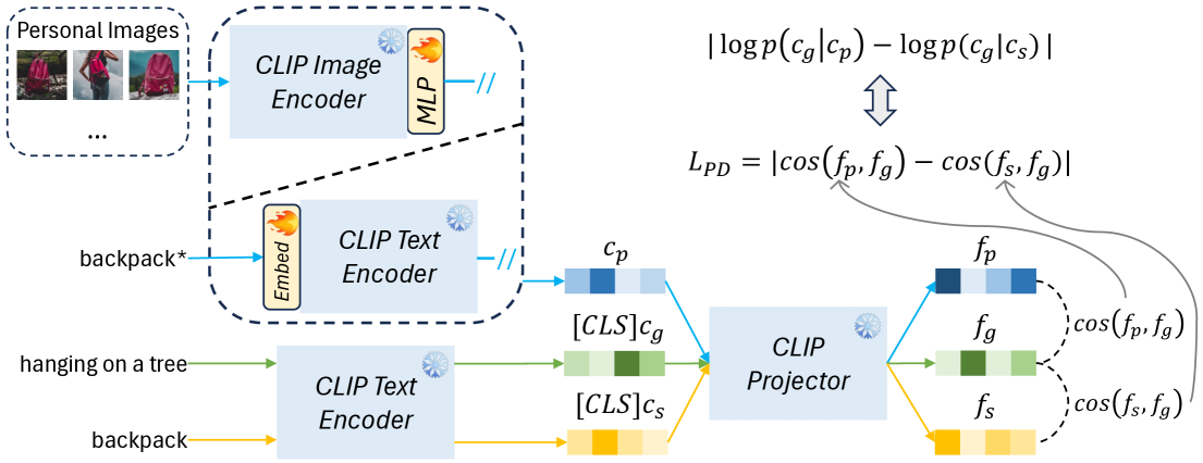
Figure 3: The calculation of the Prior Decouple Loss $\mathcal{L}_{\text{PD}}$. The purpose of $\mathcal{L}_{\text{PD}}$ is to prevent excessive prior dependence between ${\mathbf{c}}_{p}$ and general text conditions ${\mathbf{c}}_{g}$. During computation, we first use the CLIP projector to map ${\mathbf{c}}_{p}$ and ${\mathbf{c}}_{g}$ into ${\mathbf{f}}_{s}$ and ${\mathbf{f}}_{g}$, respectively, and then minimize their absolute cosine similarity.

Specifically, the prior dependence discrepancy can be equivalently written as:

$$\log r({\mathbf{c}}_{p},{\mathbf{c}}_{g})-\log r({\mathbf{c}}_{s},{\mathbf{c}}_{g})=\log\frac{p({\mathbf{c}}_{g}|{\mathbf{c}}_{p})}{p({\mathbf{c}}_{g}|{\mathbf{c}}_{s})}.$$ (12)

This equation indicates that addressing the increase in prior dependence discrepancy involves aligning the conditional probabilities $p({\mathbf{c}}_{g}|{\mathbf{c}}_{p})$ and $p({\mathbf{c}}_{g}|{\mathbf{c}}_{s})$. Unfortunately, the diffusion model does not facilitate this alignment because Eq. (12) is independent of the denoising process. Therefore, we resort to the CLIP model, guided by the following assumption:

Assumption 1.

Let $\tau$ be the temperature coefficient. For any two concepts ${\mathbf{c}}_{j}$ and ${\mathbf{c}}_{k}$, let their projections using the CLIP Projector be denoted as ${\mathbf{f}}_{j}$ and ${\mathbf{f}}_{k}$. We can then estimate $p({\mathbf{c}}_{j}|{\mathbf{c}}_{k})$ as:

$$p({\mathbf{c}}_{j}|{\mathbf{c}}_{k})\approx\frac{e^{\tau cos({\mathbf{f}}_{j},{\mathbf{f}}_{k}})}{Z_{k}},Z_{k}=\sum_{{\mathbf{f}}_{m}}e^{\tau\cos({\mathbf{f}}_{k},{\mathbf{f}}_{m})},$$ (13)

where $cos(\cdot)$ denotes the cosine similarity.

The rationale behind Assumption 1 for estimating the right-hand side of Equation (12) relies on two key aspects. Firstly, the contrastive loss used during CLIP training effectively estimates the probability that an image aligns with its corresponding caption and vice versa, mirroring the formulation presented in Equation (13). Thus, the probability of an image being associated with its caption can be interpreted as the conditional probability of the caption given the image. Secondly, ${\mathbf{c}}_{s}$ is the text embedding of the superclass (e.g., backpack) given by the CLIP Text Encoder, while ${\mathbf{c}}_{p}$ (e.g., the specifically designed red backpack in Figure 1) is often set as either a trainable text embedding in CLIP or a visual representation mapped to the CLIP text representation space. Hence, both ${\mathbf{c}}_{s}$ and ${\mathbf{c}}_{p}$ are within the CLIP text representation space, fulfilling the necessary conditions to apply Eq. (13).

Based on Assumption 1, we align $p(\mathbf{c}_{g}|\mathbf{c}_{p})$ and $p(\mathbf{c}_{g}|\mathbf{c}_{s})$ by ensuring that $cos(f_{p},f_{g})$ and $cos(f_{s},f_{g})$ are closely matched. Concretely, although estimating $Z_{p}$ and $Z_{s}$ using CLIP is intractable, we can still deduce that if $cos(f_{p},f_{g})=cos(f_{s},f_{g})$ for all ${\mathbf{c}}_{g}$, then it follows that $Z_{p}=Z_{s}$, leading to $p({\mathbf{c}}_{g}|{\mathbf{c}}_{p})=p({\mathbf{c}}_{g}|{\mathbf{c}}_{s})$ [24]. Hence, we define PDLoss as:

$$\mathcal{L}_{\text{PD}}=\mathbb{E}_{{\mathbf{c}}_{g}}[|cos({\mathbf{f}}_{p},{\mathbf{f}}_{g})-cos({\mathbf{f}}_{s},{\mathbf{f}}_{g})|],$$ (14)

The calculation of PDLoss is explained in Fig. 3.

Table 1: Quantitative results on DreamBench. The “*” indicates the performance achieved by applying variable weights to DDLoss and PDLoss for different subjects. “Params.” indicates the number of tunable parameters.

Method	CLIP-T$\uparrow$	BLIP-T$\uparrow$	CLIP-I$\uparrow$	DINO-I$\uparrow$	Params.
DreamBooth	30.3	40.3	74.0	69.3	819.7 M
Facechain-SuDe	31.4	41.6	74.3	70.5	819.7 M
DreamBooth w/ Ours	31.1 (+0.8)	42.1 (+1.8)	77.8 (+3.8)	73.5 (+4.2)	819.7 M
DreamBooth w/ Ours*	31.3 (+1.0)	42.1 (+1.8)	78.6 (+4.6)	74.4 (+5.1)	819.7 M
Custom Diffusion	34.2	45.4	62.7	56.9	18.3 M
ClassDiffusion	34.3	45.8	61.3	55.0	18.3M
Custom Diffusion w/ Ours	33.9 (-0.3)	46.4 (+1.0)	71.1 (+8.4)	65.2 (+8.3)	18.3 M
Custom Diffusion w/ Ours*	34.1 (-0.1)	46.6 (+1.2)	71.4 (+8.7)	65.6 (+8.7)	18.3 M
LoRA	31.1	42.6	78.4	74.6	12.2 M
LoRA w/ Ours	31.9 (+0.8)	43.4 (+0.8)	77.3 (-1.1)	73.4 (-1.2)	12.2 M
LoRA w/ Ours*	31.8 (+0.7)	43.0 (+0.4)	78.4 (+0.0)	75.1 (+0.5)	12.2 M
VisualEncoder	25.9	36.1	79.1	75.5	3.0 M
VisualEncoder w/ Ours	25.9 (+0.0)	35.8 (-0.3)	80.0 (+0.9)	76.0 (+0.5)	3.0 M
VisualEncoder w/ Ours*	26.3 (+0.4)	36.1 (+0.0)	80.4 (+1.3)	76.7 (+1.2)	3.0 M

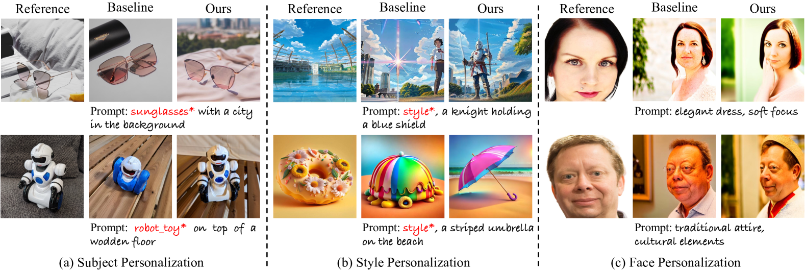
Figure 4: A comparison of the visual outcomes of subject personalization, style personalization, and face personalization, where “superclass*” denotes the personalization target.

4 Experiments

4.1 Experimental Setup

Datasets. We demonstrate the effectiveness of our proposed method across a diverse range of image personalization tasks, including subject-driven personalization, style personalization, and zero-shot face personalization. We employ the DreamBench [3] for evaluating subject personalization, the StyleBench [25] for style personalization, and the FFHQ [26] dataset for face personalization. For detailed information, please refer to Appendix A.3.

Metrics. For subject-driven personalization, we employ CLIP-T [3] and BLIP2-T [7] to assess text alignment, and CLIP-I and DINO-I [3] to evaluate subject fidelity. Concretely, CLIP-T and BLIP2-T calculate the average cosine similarity between the embeddings from prompts and generated images, utilizing CLIP and BLIP2 models, respectively. The metrics for subject fidelity, CLIP-I and DINO-I, involve computing the mean cosine similarity between embeddings of real and generated images. To mitigate background interference, we utilize the Reference Segmentation Model [27] to segment subjects in both real and generated images.

For style personalization, we similarly employ CLIP-T and BLIP-T to assess the alignment between prompts and generated images. Regarding style similarity, the Gram Matrix has been validated in numerous studies as an effective tool for capturing image style [28]. Therefore, we measure style similarity by calculating the average distance between the Gram Matrices of the reference and generated images, which we refer to as Gram-D.

For face personalization, we use CLIP-T and BLIP-T to evaluate text alignment. On the other hand, IP-Adapter [10] has demonstrated that ID embeddings extracted from ArcFace [29] are effective for assessing facial similarity. Therefore, we propose using the average cosine similarity between the ID embeddings of real and generated images as a metric to evaluate facial similarity, which we refer to as Face-Sim.

Implementation Details. We compare the proposed method with existing state-of-the-art methods, including DreamBooth [3], Custom Diffusion [4], LoRA [13], Facechain-SuDe [7], ClassDiffusion [30], and VisualEncoder [10]. We validate the effectiveness of the proposed losses in a plug-and-play manner on DreamBooth, Custom Diffusion, LoRA and VisualEncoder. We keep all designs and hyperparameters of the baselines unchanged and only integrate our proposed losses into training. Specifically, for Dreambooth and LoRA that do not train the representation of the personalization target, we exclusively apply DDLoss. For others, we apply both DDLoss and PDLoss. For more implementation details, please refer to Appendix A.4.

4.2 Subject Personalization

We compare the quantitative results of different methods on subject personalization in Tab. 1. It can be observed that: (i) The proposed DDLoss and PDLoss significantly enhance the performance of existing baselines in a plug-and-play manner, with only minor degradations occurring due to the mitigation of extreme preferences in existing methods for text alignment or personalization targets. (ii) Compared to the similar plug-and-play loss regularization methods Facechain-SuDe and ClassDiffusion, our proposed loss functions offer stronger regularization by directly optimizing concept coupling, resulting in greater performance improvements for DreamBooth. (iii) Dreambooth and Custom Diffusion rely on a regularization dataset to enhance text alignment but sacrifice subject fidelity. Conversely, Our method significantly enhance CLIP-I and DINO-I, while maintaining or improving CLIP-T and BLIP-T. The superior text alignment and subject fidelity of ACCORD is visualized in Fig. 4(a), where the “Baseline” is Dreambooth. Please refer to Fig. 6 (Appendix A.5) for more visualization results.

Table 2: Ablation study on the effects of T2I backbone, DDLoss, and PDLoss. Evaluated on the DreamBench dataset.

Method	CLIP-T	BLIP-T	CLIP-I	DINO-I
SD1.5+VisualEncoder	25.9	36.1	79.1	75.5
SD1.5+VisualEncoder+PDLoss	26.2 (+0.3)	35.9 (-0.2)	80.0 (+0.9)	75.9 (+0.4)
SD1.5+VisualEncoder+PDLoss+DDLoss	26.3 (+0.4)	36.1 (+0.0)	80.4 (+1.3)	76.7 (+1.2)
SDXL+VisualEncoder	27.1	38.4	82.8	77.6
SDXL+VisualEncoder+PDLoss	27.8 (+0.7)	39.5 (+1.1)	82.9 (+0.1)	77.4 (-0.1)
SDXL+VisualEncoder+PDLoss+DDLoss	28.3 (+1.2)	39.8 (+1.4)	83.1 (+0.3)	78.1 (+0.5)

Table 3: Quantitative results on StyleBench. The “*” denotes the performance of varying DDLoss and PDLoss weights across different styles. “Gram-D” is the gram matrix distance.

Method	CLIP-T$\uparrow$	BLIP-T$\uparrow$	Gram-D$\downarrow$
DreamBooth	31.3	46.6	42728
Facechain-SuDe	31.0	45.8	39978
DreamBooth w/ Ours	31.9 (+0.6)	47.3 (+0.7)	42524 (-0.5%)
DreamBooth w/ Ours*	32.0 (+0.7)	47.2 (+0.6)	41911 (-1.9%)
Custom Diffusion	31.2	47.7	53347
ClassDiffusion	31.8	48.4	52998
Custom Diffusion w/ Ours	31.7 (+0.5)	48.5 (+0.8)	48649 (-8.8%)
Custom Diffusion w/ Ours*	31.8 (+0.6)	48.5 (+0.8)	47852 (-10.3%)
LoRA	31.5	47.2	40451
LoRA w/ Ours	31.8 (+0.3)	47.6 (+0.4)	40918 (+0.1%)
LoRA w/ Ours*	31.6 (+0.1)	47.1 (-0.1)	38881 (-3.9%)
VisualEncoder	17.7	30.2	32176
VisualEncoder w/ Ours	17.7 (+0.0)	30.3 (+0.1)	31382 (-2.5%)
VisualEncoder w/ Ours*	18.4 (+0.7)	30.9 (+0.7)	27984 (-13.0%)

4.3 Style Personalization

We also present the performance of different methods in style personalization in Tab. 3 and Fig. 4(b). We can conclude that: (i) Our proposed DDLoss and PDLoss significantly enhance style personalization and achieve improvements across all methods in a plug-and-play manner. In Fig. 4(b), our ACCORD exhibits more precise text control compared to the “Baseline” Dreambooth. (ii) Methods relying on regularized datasets, such as DreamBooth and Custom Diffusion, perform in stark contrast to VisualEncoder. The former exhibits good text alignment but poor style fidelity, while the latter overfits to style, sacrificing text control. Our approach improves both text alignment and style fidelity simultaneously in these methods. More visualization results can be found in Appendix A.5 Fig. 7.

4.4 Face Personalization

To explore the potential of concept decoupling in zero-shot image personalization, we conduct face personalization experiments on the FFHQ dataset. Specifically, we train the IP-Adapter with and without applying our DDLoss and PDLoss based on SD1.5. The IP-Adapter employs the CLIP Vision Encoder to extract features from a reference facial image, subsequently mapping these features to 16 visual tokens using a Q-former [17]. These visual tokens are not only processed by the original cross-attention layers in the UNet alongside the textual conditions but are also utilized by the additional image attention introduced by the IP-Adapter. The quantitative results are shown in Tab. 4. It can be observed that the introduction of DDLoss and PDLoss simultaneously enhances face similarity and text alignment. In Fig. 4(c), the girl’s face generated by our method are more similar to the reference images. More visualization results can be found in Appendix A.5 Fig. 8.

4.5 Ablation Study

We investigated the impacts of the Text-to-Image backbones and the proposed PDLoss and DDLoss on personalization performance using the DreamBench dataset, as shown in Tab. 2. We have two observations: (i) The proposed loss functions are irrelevant to the T2I backbone and achieve performance improvements on both SD1.5 and SDXL. (ii) The proposed DDLoss and PDLoss both contribute to performance enhancements and can work synergistically.

Table 4: Quantitative results on FFHQ. “Face-Sim” denotes the face similarity between generated images and the reference face image.

Method	CLIP-T$\uparrow$	BLIP-T$\uparrow$	Face-Sim$\uparrow$
IP-Adapter	20.0	34.7	14.8
IP-Adapter w/ Ours	20.7 (+0.7)	34.8 (+0.1)	16.4 (+1.6)

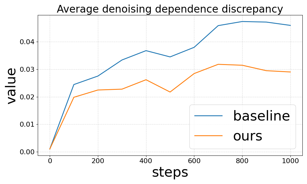
(a) Denoising dependence discrepancy

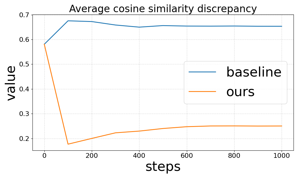
(b) Cosine similarity discrepancy

Figure 5: Visualization of the impact of DDLoss and PDLoss.

To clearly demonstrate the roles of DDLoss and PDLoss during training, we visualize their effects in Fig. 5. It can be observed that with the usage of DDLoss, the increase in denoising dependence discrepancy, $|\log r({\mathbf{c}}_{p},{\mathbf{c}}_{g}|{\mathbf{x}}_{\theta,0})-\log r({\mathbf{c}}_{p},{\mathbf{c}}_{g}|{\mathbf{x}}_{T})|$, is supressed. On the other hand, the application of PDLoss results in a reduction in the cosine similarity discrepancy $|cos({\mathbf{f}}_{p},{\mathbf{f}}_{g})-cos({\mathbf{f}}_{s},{\mathbf{f}}_{g})|$.

We further study the role of the cosine similarity target in PDLoss in Appendix A.2.

5 Conclusion

This paper addresses the challenge of concept coupling in image personalization by reformulating the problem from a statistical perspective. We decompose the concept coupling into two computable dependence discrepancies: the Denoising Dependence Discrepancy and the Prior Dependence Discrepancy. We then develop two plug-and-play loss functions: Denoising Decouple Loss and Prior Decouple Loss, that effectively mitigate these discrepancies. Our method demonstrates improvement in balancing text control with personalization fidelity, as evidenced by comprehensive experimental results. Our proposed method can be readily integrated into existing methods.

Appendix A Appendix

Table 5: Meanings of notations.

Notation	Meaning
$t$	Denoising time step, ranging from $0$ to $T$.
${\mathbf{x}}_{0}$	Clear image or its latent code.
${\mathbf{x}}_{t}$	Noisy image or its latent code at time step $t$.
${\mathbf{x}}_{T}$	Noisy image or its latent code at time step $T$, modeled as a multivariate standard Gaussian noise.
$\alpha_{t}$	Retention ratio of the original image at forward time step $t$.
$\bm{\epsilon}$	Multivariate standard Gaussian Noise.
$\theta$	Network parameters.
$\bm{\sigma}_{t}$	Standard deviation of the noisy code at time step $t$.
${\mathcal{U}}_{\theta}({\mathbf{x}}_{t},{\mathbf{c}},t)$	Output of the denoising model at time step $t-1$ given generation condition ${\mathbf{c}}$.
${\mathbf{x}}_{\theta,t}$	Shorthand for denoising output at time step $t-1$ given generation condition $({\mathbf{c}}_{p},{\mathbf{c}}_{g})$.
$\mathbb{D}$	Training set for the image personalization task.
${\mathbf{x}}^{i}$	$i$-th reference image in the training set.
${\mathbf{c}}^{i}$	$i$-th generation condition in the training set.
${\mathbf{c}}_{p}$	Personalized target condition.
${\mathbf{c}}_{g}$	General text condition.
${\mathbf{c}}_{s}$	Text condition for the superclass of ${\mathbf{c}}_{p}$.
$r({\mathbf{c}}_{p},{\mathbf{c}}_{g}|{\mathbf{x}}_{\theta,t})$	Conditional dependence coefficient for concepts ${\mathbf{c}}_{p}$ and ${\mathbf{c}}_{g}$ given generated image ${\mathbf{x}}_{\theta,t}$.
$r({\mathbf{c}}_{p},{\mathbf{c}}_{g})$	Prior dependence coefficient for concepts ${\mathbf{c}}_{p}$ and ${\mathbf{c}}_{g}$.
${\mathbf{f}}_{p},{\mathbf{f}}_{s},{\mathbf{f}}_{g}$	Projections using the CLIP Projector for ${\mathbf{c}}_{p}$, ${\mathbf{c}}_{s}$, and ${\mathbf{c}}_{g}$.

A.1 Proof of Theorem 3.3

According to the definition of $r({\mathbf{c}}_{p},{\mathbf{c}}_{g}|{\mathbf{x}}_{\theta,t-1})$:

$$r({\mathbf{c}}_{p},{\mathbf{c}}_{g}|{\mathbf{x}}_{\theta,t-1})=\frac{p({\mathbf{c}}_{p},{\mathbf{c}}_{g}|{\mathbf{x}}_{\theta,t-1})}{p({\mathbf{c}}_{p}|{\mathbf{x}}_{\theta,t-1})p({\mathbf{c}}_{g}|{\mathbf{x}}_{\theta,t-1})},$$ (15)

the core of computing $\log r({\mathbf{c}}_{p},{\mathbf{c}}_{g}|{\mathbf{x}}_{\theta,t-1})$ lies in the computation of $p(\hat{\mathbf{c}}|{\mathbf{x}}_{\theta,t-1})$, where $\hat{\mathbf{c}}$ is an arbitrary condition. By applying Bayes’ theorem, we have:

$$p(\hat{\mathbf{c}}|{\mathbf{x}}_{\theta,t-1})=p(\hat{\mathbf{c}}|{\mathbf{x}}_{\theta,t-1},{\mathbf{x}}_{\theta,t})=\frac{p(\hat{\mathbf{c}}|{\mathbf{x}}_{\theta,t})p({\mathbf{x}}_{\theta,t-1}|{\mathbf{x}}_{\theta,t},\hat{\mathbf{c}})}{p({\mathbf{x}}_{\theta,t-1}|{\mathbf{x}}_{\theta,t})}.$$ (16)

The first equation holds because the computation of ${\mathbf{x}}_{\theta,t-1}$ relies on ${\mathbf{x}}_{\theta,t}$:

$${\mathbf{x}}_{\theta,t-1}={\mathcal{U}}_{\theta}({\mathbf{x}}_{t},({\mathbf{c}}_{p},{\mathbf{c}}_{g}),t),\quad{\mathbf{x}}_{t}={\mathbf{x}}_{\theta,t}+\bm{\sigma}_{t+1}\bm{\epsilon}_{t+1},\quad\bm{\epsilon}_{t+1}\sim{\mathcal{N}}(0,I),$$ (17)

where $\bm{\sigma}_{t+1}$ is the standard derivation of the noisy code at time step $t+1$.

Next, we compute $p({\mathbf{x}}_{\theta,t-1}|{\mathbf{x}}_{\theta,t},\hat{\mathbf{c}})$ and $p({\mathbf{x}}_{\theta,t-1}|{\mathbf{x}}_{\theta,t})$. In diffusion models, $p({\mathbf{x}}_{\theta,t-1}|{\mathbf{x}}_{\theta,t},\hat{\mathbf{c}})$ is a Gaussian distribution (cf. Section 3.1) that can be parameterized as:

$$p({\mathbf{x}}_{\theta,t-1}|{\mathbf{x}}_{\theta,t},\hat{\mathbf{c}})={\mathcal{N}}\big{(}{\mathbf{x}}_{\theta,t-1};{\mathcal{U}}_{\theta}({\mathbf{x}}_{\theta,t},\hat{\mathbf{c}},t),\sigma_{t}^{2}{\bm{I}}\big{)}=\exp(C-\frac{\|{\mathbf{x}}_{\theta,t-1}-{\mathcal{U}}_{\theta}({\mathbf{x}}_{\theta,t},\hat{\mathbf{c}},t)\|^{2}}{2\bm{\sigma}_{t}^{2}}),$$ (18)

where $C$ is a constant. We then substitue Eq. (17) into Eq. (18) and obtain:

$$p({\mathbf{x}}_{\theta,t-1}|{\mathbf{x}}_{\theta,t},\hat{\mathbf{c}})=\exp(C-\frac{\|{\mathcal{U}}_{\theta}({\mathbf{x}}_{t},({\mathbf{c}}_{p},{\mathbf{c}}_{g}),t)-{\mathcal{U}}_{\theta}({\mathbf{x}}_{\theta,t},\hat{\mathbf{c}},t)\|^{2}}{2\bm{\sigma}_{t}^{2}}),$$ (19)

Note that $\hat{\mathbf{c}}$ is an arbitrary condition, $p({\mathbf{x}}_{\theta,t-1}|{\mathbf{x}}_{\theta,t})$ can be obtained by setting $\hat{\mathbf{c}}=\varnothing$. Therefore, we substitute Eq. (19) into Eq. (16) and obtain:

$$\log p(\hat{\mathbf{c}}|{\mathbf{x}}_{\theta,t-1})-\log p(\hat{\mathbf{c}}|{\mathbf{x}}_{\theta,t})=\frac{1}{2\bm{\sigma}_{t}^{2}}\Big{[}\|{\mathcal{U}}_{\theta}({\mathbf{x}}_{t},({\mathbf{c}}_{p},{\mathbf{c}}_{g}),t)-{\mathcal{U}}_{\theta}({\mathbf{x}}_{\theta,t},\varnothing,t)\|^{2}-\|{\mathcal{U}}_{\theta}({\mathbf{x}}_{t},({\mathbf{c}}_{p},{\mathbf{c}}_{g}),t)-{\mathcal{U}}_{\theta}({\mathbf{x}}_{\theta,t},\hat{\mathbf{c}},t)\|^{2}\Big{]}$$ (20)

Finally, by substituting Eq. (20) into the definition of $r({\mathbf{c}}_{p},{\mathbf{c}}_{g}|{\mathbf{x}}_{\theta,t-1})$ (15), we obtain:

$$\,\log r({\mathbf{c}}_{p},{\mathbf{c}}_{g}|{\mathbf{x}}_{\theta,t-1})-\log r({\mathbf{c}}_{p},{\mathbf{c}}_{g}|{\mathbf{x}}_{\theta,t})$$

$$= \,\frac{1}{2\bm{\sigma}_{t}^{2}}\Big{[}\|{\mathcal{U}}_{\theta}\big{(}{\mathbf{x}}_{t},({\mathbf{c}}_{p},{\mathbf{c}}_{g}),t\big{)}-{\mathcal{U}}_{\theta}\big{(}{\mathbf{x}}_{\theta,t},{\mathbf{c}}_{p},t\big{)}\|^{2}$$

$$\,+\|{\mathcal{U}}_{\theta}\big{(}{\mathbf{x}}_{t},({\mathbf{c}}_{p},{\mathbf{c}}_{g}),t\big{)}-{\mathcal{U}}_{\theta}\big{(}{\mathbf{x}}_{\theta,t},{\mathbf{c}}_{g},t\big{)}\|^{2}$$

$$\,-\|{\mathcal{U}}_{\theta}\big{(}{\mathbf{x}}_{t},({\mathbf{c}}_{p},{\mathbf{c}}_{g}),t\big{)}-{\mathcal{U}}_{\theta}\big{(}{\mathbf{x}}_{\theta,t},\varnothing,t\big{)}\|^{2}\Big{]}.$$ (21)

This closes the proof.

A.2 Ablation Study on the impact of cosine similarity target

To minimize concept coupling in Eq. (4), we align the cosine similarity $cos({\mathbf{f}}_{p},{\mathbf{f}}_{g})$ with $cos({\mathbf{f}}_{s},{\mathbf{f}}_{g})$ in Eq. (14). To further understand the role of the cosine similarity target in PDLoss, we study its impact in Tab. 6. It is observed that as the cosine similarity target decreases, metrics related to text alignment, namely CLIP-T and BLIP-T, improve, whereas metrics associated with personalization fidelity, such as CLIP-I and DINO-I, decline. This observation aligns with Assumption 1. A lower cosine similarity indicates a reduced $p({\mathbf{c}}_{g}|{\mathbf{c}}_{p})$, implying that ${\mathbf{c}}_{p}$ is less likely to interfere with other text concepts. However, if the similarity between ${\mathbf{c}}_{p}$ and ${\mathbf{c}}_{g}$ decreases excessively, it becomes challenging for ${\mathbf{c}}_{p}$ to maintain inherent relationships with its superclass and other concepts, thereby impairing personalization fidelity. Consequently, setting the cosine similarity target as $cos({\mathbf{f}}_{s},{\mathbf{f}}_{g})$ achieves a balance between text alignment and personalization fidelity.

Table 6: Ablation study on the optimization target of cosine similarity $cos({\mathbf{f}}_{p},{\mathbf{f}}_{g})$ in PDLoss.

Cosine similarity target	CLIP-T$\uparrow$	BLIP-T$\uparrow$	CLIP-I$\uparrow$	DINO-I$\uparrow$
VisualEncoder wo/ Ours	25.9	36.1	79.1	75.5
$cos({\mathbf{f}}_{s},{\mathbf{f}}_{g})$ (typically $>0$)	26.2 (+0.3)	35.9 (-0.2)	80.0 (+0.9)	75.9 (+0.4)
$0$	26.4 (+0.4)	36.8 (+0.7)	79.9 (+0.8)	75.5 (+0.0)
$-1$	27.7 (+1.8)	38.4 (+2.3)	77.6 (-1.5)	73.3 (-2.2)

A.3 Detailed Dataset Information

We utilize the DreamBench [3] dataset to compare the subject-driven personalization capabilities of different methods. DreamBench contains 30 subjects across 15 categories, of which 9 are animals, with each subject having 4-6 images. For style personalization, we employ StyleBench [25], which focuses on style transfer tasks and includes 73 distinct styles, each style comprising 5 or more reference images. Furthermore, to validate the effectiveness of our proposed losses for zero-shot image personalization, we conducted face personalization experiments on the FFHQ [26] dataset. FFHQ is a dataset of 70,000 high-quality face images, offering substantial diversity in age, ethnicity, background, etc. We employ Insightface [29] to detect over 40,000 images containing only a single face, and exclusively use these images for training and testing.

A.4 More Implementation Details

The baseline VisualEncoder [10] is a simplified version of IP-Adapter that retains the CLIP Image Encoder-based Visual Encoder, as depicted in Fig. 3, omitting the image-specific Cross Attention. This design implies that only the MLP at the end of the CLIP Image Encoder is trainable, and the personalization relies entirely on the visual embeddings ${\mathbf{c}}_{p}$ extracted by the visual encoder. We found it to serve as a strong parameter-efficient baseline. We utilize the official implementation of Facechain-SuDe while implementing other baselines and our proposed method using open-source library diffusers [31]. All methods employ the DDIM sampler, a guidance scale of 7.5, and 50 inference steps during evaluation.

The different training paradigms of the various baselines necessitate distinct weighting for DDLoss and PDLoss. After tuning the loss weights using validation prompts, we find that, in general, a DDLoss weight between 0.1 and 0.3 suffices, while a PDLoss weight between 0.001 and 0.003 is adequate. We train all methods for 1000 steps on each subject or style and display the results of the best-performing step. It is noteworthy that users can adjust the loss weights in practice to achieve optimal results due to the automatic computation of CLIP-T, BLIP-T, CLIP-I, DINO-I, Gram-D, and Face-Sim.

A.5 More Visualization Results

We provide more visualization results in Fig. 6, 7 and 8. For subject and style personalization, the “Baseline” is Dreambooth. For face personalization, the “Baseline” is IP-Adapter. The following observations can be made: (1) Our method demonstrates superior text alignment compared to the baseline. Specifically, in the first, second, and third columns of Fig. 6, our method successfully generated a snowy scene, a wheat field, and a purple bowl, whereas the baseline model did not. In the first, third, and fourth columns of Fig. 7, our approach successfully produced images of a pirate, a lion, and a snowy landscape. Finally, in the third and fourth columns of Fig. 8, our method generated a cityscape background and cultural elements according to the prompts. (2) Our method better preserves personalization fidelity. In the fourth, fifth, and sixth rows of Fig. 6, our method generates subjects that more resemble the reference images, whereas the baseline either produces an unrelated cat or anomalies such as four eyes and a black dog back. In the second and sixth rows of Fig. 7, the images generated by our method exhibit styles more closely aligned with the reference styles, namely the clay style and fauvism style. Finally, in all columns of Fig. 8, the faces generated by our method more closely resemble the reference faces.

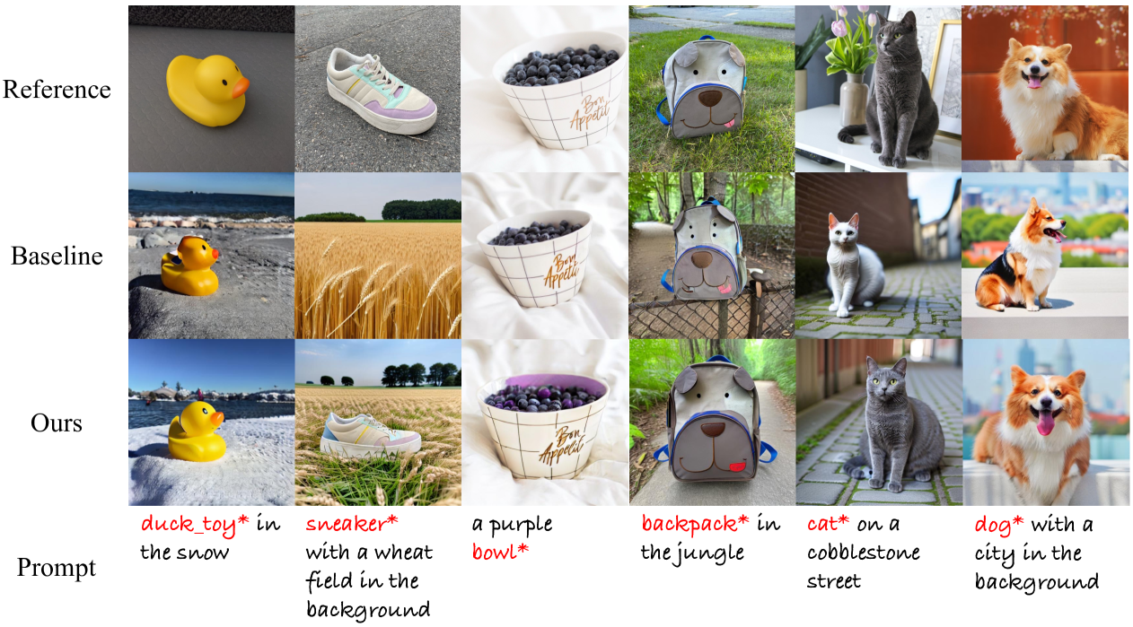
Figure 6: A comparison of the visual outcomes of subject personalization, where “superclass*” denotes the personalization target.

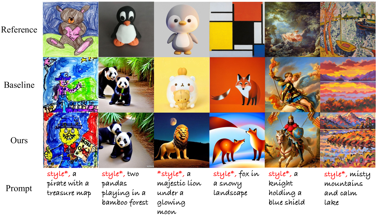
Figure 7: A comparison of the visual outcomes of style personalization, where “style*” denotes the personalization target style.

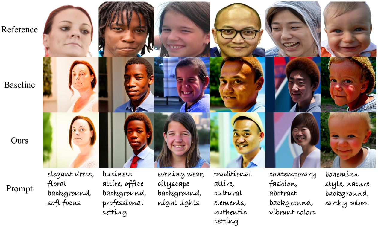
Figure 8: A comparison of the visual outcomes of face personalization.

References

- [1] Jonathan Ho, Ajay Jain, and Pieter Abbeel. Denoising diffusion probabilistic models. Advances in neural information processing systems, 33:6840–6851, 2020.
- [2] Robin Rombach, Andreas Blattmann, Dominik Lorenz, Patrick Esser, and Björn Ommer. High-resolution image synthesis with latent diffusion models. In Proceedings of the IEEE/CVF conference on computer vision and pattern recognition, pages 10684–10695, 2022.
- [3] Nataniel Ruiz, Yuanzhen Li, Varun Jampani, Yael Pritch, Michael Rubinstein, and Kfir Aberman. Dreambooth: Fine tuning text-to-image diffusion models for subject-driven generation. In Proceedings of the IEEE/CVF conference on computer vision and pattern recognition, pages 22500–22510, 2023.
- [4] Nupur Kumari, Bingliang Zhang, Richard Zhang, Eli Shechtman, and Jun-Yan Zhu. Multi-concept customization of text-to-image diffusion. In Proceedings of the IEEE/CVF Conference on Computer Vision and Pattern Recognition, pages 1931–1941, 2023.
- [5] Ligong Han, Yinxiao Li, Han Zhang, Peyman Milanfar, Dimitris Metaxas, and Feng Yang. Svdiff: Compact parameter space for diffusion fine-tuning. In Proceedings of the IEEE/CVF International Conference on Computer Vision, pages 7323–7334, 2023.
- [6] Zeju Qiu, Weiyang Liu, Haiwen Feng, Yuxuan Xue, Yao Feng, Zhen Liu, Dan Zhang, Adrian Weller, and Bernhard Schölkopf. Controlling text-to-image diffusion by orthogonal finetuning. Advances in Neural Information Processing Systems, 36:79320–79362, 2023.
- [7] Pengchong Qiao, Lei Shang, Chang Liu, Baigui Sun, Xiangyang Ji, and Jie Chen. Facechain-sude: Building derived class to inherit category attributes for one-shot subject-driven generation. In Proceedings of the IEEE/CVF Conference on Computer Vision and Pattern Recognition, pages 7215–7224, 2024.
- [8] Yeji Song, Jimyeong Kim, Wonhark Park, Wonsik Shin, Wonjong Rhee, and Nojun Kwak. Harmonizing visual and textual embeddings for zero-shot text-to-image customization. arXiv preprint arXiv:2403.14155, 2024.
- [9] Rinon Gal, Yuval Alaluf, Yuval Atzmon, Or Patashnik, Amit Haim Bermano, Gal Chechik, and Daniel Cohen-or. An image is worth one word: Personalizing text-to-image generation using textual inversion. In The Eleventh International Conference on Learning Representations, 2022.
- [10] Hu Ye, Jun Zhang, Sibo Liu, Xiao Han, and Wei Yang. Ip-adapter: Text compatible image prompt adapter for text-to-image diffusion models. arXiv preprint arXiv:2308.06721, 2023.
- [11] Alec Radford, Jong Wook Kim, Chris Hallacy, Aditya Ramesh, Gabriel Goh, Sandhini Agarwal, Girish Sastry, Amanda Askell, Pamela Mishkin, Jack Clark, et al. Learning transferable visual models from natural language supervision. In International conference on machine learning, pages 8748–8763. PMLR, 2021.
- [12] Haoming Lu, Hazarapet Tunanyan, Kai Wang, Shant Navasardyan, Zhangyang Wang, and Humphrey Shi. Specialist diffusion: Plug-and-play sample-efficient fine-tuning of text-to-image diffusion models to learn any unseen style. In Proceedings of the IEEE/CVF Conference on Computer Vision and Pattern Recognition, pages 14267–14276, 2023.
- [13] Edward J Hu, Yelong Shen, Phillip Wallis, Zeyuan Allen-Zhu, Yuanzhi Li, Shean Wang, Lu Wang, and Weizhu Chen. Lora: Low-rank adaptation of large language models. arXiv preprint arXiv:2106.09685, 2021.
- [14] Jun Ahn Hyung, Jaeyo Shin, and Jaegul Choo. Magicapture: High-resolution multi-concept portrait customization. In AAAI Conference on Artificial Intelligence, 2023.
- [15] Jing Shi, Wei Xiong, Zhe Lin, and Hyun Joon Jung. Instantbooth: Personalized text-to-image generation without test-time finetuning. In Proceedings of the IEEE/CVF Conference on Computer Vision and Pattern Recognition, pages 8543–8552, 2024.
- [16] Dongxu Li, Junnan Li, and Steven Hoi. Blip-diffusion: Pre-trained subject representation for controllable text-to-image generation and editing. Advances in Neural Information Processing Systems, 36, 2024.
- [17] Junnan Li, Dongxu Li, Silvio Savarese, and Steven Hoi. Blip-2: bootstrapping language-image pre-training with frozen image encoders and large language models. In Proceedings of the 40th International Conference on Machine Learning, ICML’23. JMLR.org, 2023.
- [18] Yuxiang Wei, Yabo Zhang, Zhilong Ji, Jinfeng Bai, Lei Zhang, and Wangmeng Zuo. Elite: Encoding visual concepts into textual embeddings for customized text-to-image generation. In Proceedings of the IEEE/CVF International Conference on Computer Vision, pages 15943–15953, 2023.
- [19] Qixun Wang, Xu Bai, Haofan Wang, Zekui Qin, Anthony Chen, Huaxia Li, Xu Tang, and Yao Hu. Instantid: Zero-shot identity-preserving generation in seconds. arXiv preprint arXiv:2401.07519, 2024.
- [20] Haofan Wang, Matteo Spinelli, Qixun Wang, Xu Bai, Zekui Qin, and Anthony Chen. Instantstyle: Free lunch towards style-preserving in text-to-image generation. arXiv preprint arXiv:2404.02733, 2024.
- [21] Dustin Podell, Zion English, Kyle Lacey, Andreas Blattmann, Tim Dockhorn, Jonas Müller, Joe Penna, and Robin Rombach. Sdxl: Improving latent diffusion models for high-resolution image synthesis. In The Twelfth International Conference on Learning Representations, 2023.
- [22] Zhe Chen, Jiannan Wu, Wenhai Wang, Weijie Su, Guo Chen, Sen Xing, Muyan Zhong, Qinglong Zhang, Xizhou Zhu, Lewei Lu, et al. Internvl: Scaling up vision foundation models and aligning for generic visual-linguistic tasks. In Proceedings of the IEEE/CVF Conference on Computer Vision and Pattern Recognition, pages 24185–24198, 2024.
- [23] Jonathan Ho and Tim Salimans. Classifier-free diffusion guidance. In NeurIPS 2021 Workshop on Deep Generative Models and Downstream Applications, 2021.
- [24] Wonpyo Park, Dongju Kim, Yan Lu, and Minsu Cho. Relational knowledge distillation. In Proceedings of the IEEE Conference on Computer Vision and Pattern Recognition, pages 3967–3976, 2019.
- [25] Gao Junyao, Liu Yanchen, Sun Yanan, Tang Yinhao, Zeng Yanhong, Chen Kai, and Zhao Cairong. Styleshot: A snapshot on any style. arXiv preprint arxiv:2407.01414, 2024.
- [26] Tero Karras, Samuli Laine, and Timo Aila. A style-based generator architecture for generative adversarial networks. IEEE Transactions on Pattern Analysis and Machine Intelligence, 43(12):4217–4228, 2021.
- [27] Yuxuan Zhang, Tianheng Cheng, Rui Hu, Lei Liu, Heng Liu, Longjin Ran, Xiaoxin Chen, Wenyu Liu, and Xinggang Wang. Evf-sam: Early vision-language fusion for text-prompted segment anything model. arXiv preprint arxiv:2406.20076, 2024.
- [28] Leon A. Gatys, Alexander S. Ecker, and Matthias Bethge. Image style transfer using convolutional neural networks. In 2016 IEEE Conference on Computer Vision and Pattern Recognition (CVPR), pages 2414–2423, 2016.
- [29] Jiankang Deng, Jia Guo, Niannan Xue, and Stefanos Zafeiriou. Arcface: Additive angular margin loss for deep face recognition. In Proceedings of the IEEE/CVF Conference on Computer Vision and Pattern Recognition, pages 4690–4699, 2019.
- [30] Jiannan Huang, Jun Hao Liew, Hanshu Yan, Yuyang Yin, Yao Zhao, and Yunchao Wei. Classdiffusion: More aligned personalization tuning with explicit class guidance, 2024.
- [31] Patrick von Platen, Suraj Patil, Anton Lozhkov, Pedro Cuenca, Nathan Lambert, Kashif Rasul, Mishig Davaadorj, Dhruv Nair, Sayak Paul, William Berman, Yiyi Xu, Steven Liu, and Thomas Wolf. Diffusers: State-of-the-art diffusion models. https://github.com/huggingface/diffusers, 2022.